Circumbinary discs: Numerical and physical behaviour

Abstract

Aims. Discs around a central binary system play an important role in star and planet formation and in the evolution of galactic discs. These circumbinary discs are strongly disturbed by the time varying potential of the binary system and display a complex dynamical evolution that is not well understood. Our goal is to investigate the impact of disc and binary parameters on the dynamical aspects of the disc.

Methods. We study the evolution of circumbinary discs under the gravitational influence of the binary using two-dimensional hydrodynamical simulations. To distinguish between physical and numerical effects we apply three hydrodynamical codes. First we analyse in detail numerical issues concerning the conditions at the boundaries and grid resolution. We then perform a series of simulations with different binary parameters (eccentricity, mass ratio) and disc parameters (viscosity, aspect ratio) starting from a reference model with Kepler-16 parameters.

Results. Concerning the numerical aspects we find that the length of the inner grid radius and the binary semi-major axis must be comparable, with free outflow conditions applied such that mass can flow onto the central binary. A closed inner boundary leads to unstable evolutions.

We find that the inner disc turns eccentric and precesses for all investigated physical parameters. The precession rate is slow with periods ($T_{\mathrm{prec}}$) starting at around 500 binary orbits ($T_{\mathrm{bin}}$) for high viscosity and a high aspect ratio $H/R$ where the inner hole is smaller and more circular. Reducing $\alpha$ and $H/R$ increases the gap size and $T_{\mathrm{prec}}$ reaches 2500 $T_{\mathrm{bin}}$. For varying binary mass ratios $q_{\mathrm{bin}}$ the gap size remains constant, whereas $T_{\mathrm{prec}}$ decreases with increasing $q_{\mathrm{bin}}$.

For varying binary eccentricities $e_{\mathrm{bin}}$ we find two separate branches in the gap size and eccentricity diagram. The bifurcation occurs at around $e_{\mathrm{crit}}\approx 0.18$ where the gap is smallest with the shortest $T_{\mathrm{prec}}$. For $e_{\mathrm{bin}}$ lower and higher than $e_{\mathrm{crit}}$, the gap size and $T_{\mathrm{prec}}$ increase. Circular binaries create the most eccentric discs.

1 Introduction

Circumbinary discs are accretion discs that orbit a binary system that consists for example of a binary star or a binary black hole system. A very prominent example of a circumbinary disc orbiting two stars is the system GG Tau. Due to the large star separation, the whole system (stars and disc) can be directly imaged by interferometric methods (Guilloteau et al., 1999). Later data yielded constraints on the size of the dust in the system and have indicated that the central binary may consist of multiple stellar systems (see Andrews et al. (2014), Di Folco et al. (2014) and references therein). More recent observations have pointed to possible planet formation (Dutrey et al., 2014) and streamers from the disc onto the stars (Yang et al., 2017). A summary of the properties of the GG Tau system is given in Dutrey et al. (2016).

An additional important clue for the existence and importance of circumbinary discs is given by the observed circumbinary planets. These are planetary systems where the planets do not orbit one star, but instead orbit a binary star system. These systems have been detected in recent years by the Kepler Space Mission and have inspired an intense research activity. The first such circumbinary planet, Kepler-16b, orbits its host system consisting of a K-type main-sequence star and an M-type red dwarf, in what is known as a P-type orbit with a semi-major axis of $0.7048\text{\,}\mathrm{a}\mathrm{u}$ and a period of $228.7$ days (Doyle et al., 2011). Presently there are ten Kepler circumbinary planets known and a summary of the properties of the first five systems discovered is given in Welsh et al. (2014) . The observations have shown that in these systems the stars are mutually eclipsing each other, as well as the planets. The simultaneous eclipses of several objects is a clear indication of the flatness of the system because the orbital plane of the binary star has to coincide nearly exactly with the orbital plane of the planet. In this respect these systems are flatter than our own solar system. Because planets form in discs, the original protoplanetary disc in these systems had to orbit around both stars, hence it must have been a circumbinary disc that was also coplanar with respect to the orbital plane of the central binary.

In addition to their occurrence around younger stars, circumbinary discs are believed to orbit supermassive black hole binaries in the centres of galaxies (Begelman et al., 1980), where they may play an important role in the evolution of the host galaxies (Armitage & Natarajan, 2002). In the early phase of the Universe there were many more close encounters between the young galaxies that alread had black holes in their centres. The gravitational tidal forces between them often resulted in new merged objects that consisted of a central black hole binary surrounded by a large circumbinary disc (see e.g. Cuadra et al., 2009; Lodato et al., 2009, and references therein). The dynamical behaviour of such a system is very similar to the one described above, where we have two stars instead of black holes.

To understand the dynamics of discs around young binary stars such as GG Tau or the planet formation process in circumbinary discs or the dynamical evolution of a central black hole binary in a galaxy, it is important to understand in detail the behaviour of a disc orbiting a central binary. The strong gravitational perturbation by the binary generates spiral waves in the disc; these waves transport energy and angular momentum from the binary to the disc (Pringle, 1991) and subseqently alter the evolution of the binary (Artymowicz et al., 1991). The most important impact of the angular momentum transfer to the disc is the formation of an inner cavity in the disc with a very low density whose size depends on disc parameters (such as viscosity or scale height) and on the binary properties (mass ratio, eccentricity) (Artymowicz & Lubow, 1994).

The numerical simulation of these circumbinary discs is not trivial and over the years several attempts have been made. The first simulations of circumbinary discs used the smoothed particle hydrodynamics (SPH) method, a Lagrangian method where the fluid is modelled as individual particles (Artymowicz & Lubow, 1996). On the one hand, this method has the advantage that the whole system can be included in the computational domain and hence the accretion onto the single binary components can be studied. On the other hand, because of the finite mass of the SPH-particles, the maximum density contrast that can be resolved is limited.

Later Rozyczka & Laughlin (1997) simulated circumbinary discs with the help of a finite difference method on a polar grid. The grid allowed for a much larger range in mass resolution than the SPH codes used to date. A polar grid is well suited for the outer parts of a disc, but suffers from the fact that there will always be an inner hole in the computational domain since the minimum radius $R_{\mathrm{min}}$ cannot be made arbitrarily small. Decreasing the minimum radius will also strongly reduce the required numerical time step, rendering long simulations unfeasible. But since circumbinary disc simulations have to be simulated for tens of thousands of binary orbits to reach a quasi-steady state, the minimum radius is often chosen such that the motion of the central stars is not covered by the computational domain, and the mass transfer from the disc to the binary cannot be studied.

Günther & Kley (2002) used a special dual-grid technique to use the best of the two worlds, the high resolution of the grid codes and the coverage of the whole domain of the particle codes. For the outer disc they used a polar grid and they overlaid the central hole with a Cartesian grid. In this way it was possible to study the complex interaction between the binary and the disc in greater detail. All these simulations indicated that despite the formation of an inner gap, material can enter the inner regions around the stars crossing the gap through stream like features to eventually become accreted onto the stars and influence their evolution (Bate et al., 2002).

Another interesting feature of circumbinary discs concerns their eccentricity. As shown in hydrodynamical simulations for planetary mass companions, discs develop a global eccentric mode even for circular binaries (Papaloizou et al., 2001). The eccentricity is confined to the inner disc region and shows a very slow precession (Kley & Dirksen, 2006). These results were confirmed for equal mass binaries on circular orbits (MacFadyen & Milosavljević, 2008). The disc eccentricity is excited by the 1:3 outer eccentric Lindblad resonance (Lubow, 1991; Papaloizou et al., 2001), which is operative for a sufficiently cleared out gap. For circular binaries a transition, in the disc structure from more circular to eccentric is thought to occur for a mass ratio of secondary to primary above 1/25 (D’Orazio et al., 2016). However, this appears to contradict the mentioned results by Papaloizou et al. (2001) and Kley & Dirksen (2006) who show that this transition already occurs for a secondary in the planet mass regime with details depending on disc parameters such as pressure and viscosity.

Driven by the observation of planets orbiting eccentric binary stars and the possibility of studying eccentric binary black holes, a large number of numerical simulations have been performed over the last few years dealing with discs around eccentric central binaries (e.g. Pierens & Nelson, 2013; Kley & Haghighipour, 2014; Dunhill et al., 2015). The recent simulations of circumbinary discs by Pierens & Nelson (2013), Kley & Haghighipour (2014) and Lines et al. (2015) used grid-based numerical methods on a polar grid with an inner hole. This raises questions about the location and imposed boundary conditions at the innermost grid radius $R_{\mathrm{min}}$. In particular, the value of $R_{\mathrm{min}}$ must be small enough to capture the development of the disc eccentricity through gravitational interaction between the binary and the disc, especially through the 1:3 Lindblad resonance (Pierens & Nelson, 2013). Therefore $R_{\mathrm{min}}$ has to be chosen in a way that all important resonances lie inside the computational domain.

In addition to the position of the inner boundary, there is no common agreement on which numerical boundary condition better describes the disc. In simulations concerning circumbinary planets mainly two types of boundary conditions are used: closed inner boundaries (Pierens & Nelson, 2013; Lines et al., 2015) that do not allow for mass flow onto the central binary, and outflow boundaries (Kley & Haghighipour, 2014, 2015) that do allow for accretion onto the binary. While Lines et al. (2015) do not find a significant difference between these two cases, Kley & Haghighipour (2014) see a clear impact on the surface density profile, and they were also able to construct discs with (on average) constant mass flow through the disc, which is not possible for closed boundaries. Driven by these discussions in the literature we decided to perform dedicated numerical studies to test the impact of the location of $R_{\mathrm{min}}$, the chosen boundary condition, and other numerical aspects in more detail. During our work we became aware of other simulations that were tackling similar problems. In October 2016 alone three publications appeared on astro-ph that described numerical simulations of circumbinary discs (Fleming & Quinn, 2017; Miranda et al., 2017; Mutter et al., 2017). While the first paper considered SPH-simulations, in the latter two papers grid-codes were used and in both the boundary condition at $R_{\mathrm{min}}$ is discussed.

In our paper we start out with numerical considerations and investigate the necessary conditions at the inner boundary in detail, and we discuss aspects of the other recent results in the presentation of our findings below. Additionally, we present a detailed parameter study of the dynamical behaviour of circumbinary discs as a function of binary and disc properties.

We organised this paper in the following way. In Sect. 2 we describe the numerical and physical setup of our circumbinary simulations. In Sect. 3 we briefly describe the numerical methods of the different codes we used for our simulations. In Sect. 4 we examine the disc structure by varying the inner boundary condition and its location. The influence of different binary parameters are examined in Sect. 5. Different disc parameters and their influence are studied in Sect. 6. Finally we summarise and discuss our results in Sect. 7.

2 Model setup

To study the evolution of circumbinary discs we perform locally isothermal hydrodynamical simulations. As a reference system we consider a binary star having the properties of Kepler-16, whose dynamical parameters are presented in Table 1. This system has a typical mass ratio and a moderate eccentricity of the orbit, and it has been studied frequently in the literature. In our parameter study we start from this reference system and vary the different aspects systematically.

Table 1: Orbital parameters of the Kepler-16 system.

$M_{A}\;[M_{\sun}]$	$M_{B}\;[M_{\sun}]$	$q_{\mathrm{bin}}$	$a_{\mathrm{bin}}\;[\mathrm{au}]$	$e_{\mathrm{bin}}$	$T_{\mathrm{bin}}\;[\mathrm{d}]$
0.69	0.20	0.29	0.22	0.16	41.08

2.1 Physics and equations

Inspired by the flatness of the observed circumbinary planetary systems, for example in the Kepler-16 system the motion takes place in single plane to within $0.5^{\circ}$ (Doyle et al., 2011), we make the following two assumptions:

1. The vertical thickness $H$ of the disc is small compared to the distance from the centre $R$;

2. There is no vertical motion.

It is therefore acceptable to reduce the problem to two dimensions by vertically averaging the hydrodynamical equations. In this case it is meaningful to work in cylindrical coordinates $(R,\varphi,z)$ and the averaging process is done in the $z$-direction. Furthermore, we choose the centre of mass of the binary as the origin of our coordinate system with the vertical axis aligned with the rotation axis of the binary. The averaged hydrodynamical equations are then given by

$$\frac{\partial}{\partial t}\Sigma+\bm{\mathrm{\nabla}}\cdot\left(\Sigma\bm{\mathrm{u}}\right)=0\,,$$ (1)

$$\frac{\partial}{\partial t}\left(\Sigma\bm{\mathrm{u}}\right)+\bm{\mathrm{\nabla}}\cdot\left(\Sigma\bm{\mathrm{u}}\otimes\bm{\mathrm{u}}-\bm{\mathrm{\Pi}}\right)=-\bm{\mathrm{\nabla}}P-\Sigma\bm{\mathrm{\nabla}}\Phi\,,$$ (2)

where $\Sigma=\int_{-\infty}^{\infty}\varrho\,\mathrm{d}z$ is the surface density, $P=\int_{-\infty}^{\infty}p\,\mathrm{d}z$ the vertically integrated pressure, and $\bm{\mathrm{u}}=(u_{R},u_{\varphi})^{\mathrm{T}}$ the two-dimensional velocity vector. We close this system of equations with a locally isothermal equation of state

$$P=c_{\mathrm{s}}^{2}(R)\Sigma\,,$$ (3)

with the local sound speed $c_{\mathrm{s}}(R)$.

The gravitational potential $\Phi$ of both stars is given by

$$\Phi=-\sum_{k=1}^{2}\frac{GM_{k}}{\left[\left(\bm{\mathrm{R}}-\bm{\mathrm{R}}_{k}\right)^{2}+\left(\varepsilon H\right)^{2}\right]^{1/2}}\,.$$ (4)

Here $M_{k}$ denotes the mass of the $k$-th star, $G$ is the gravitational constant, and $\bm{\mathrm{R}}-\bm{\mathrm{R}}_{k}$ a vector from a point in the disc to the primary or secondary star. From a numerical point of view, the smoothing factor $\varepsilon H$ is not necessary if the orbit of the binary is not inside the computational domain. We use this smoothing factor to account for the vertically extended three-dimensional disc in our two-dimensional case (Müller et al., 2012). For all simulations we use a value of $\varepsilon=0.6$.

In our simulations with no bulk viscosity the viscous stress tensor $\bm{\mathrm{\Pi}}$ is given in tensor notation by

$$\bm{\mathrm{\Pi}}_{ij}=2\eta\left[\frac{1}{2}\left(u_{j;i}+u_{i;j}\right)-\frac{1}{3}\delta_{ij}(\bm{\mathrm{\nabla}}\cdot\bm{\mathrm{u}})\right]\,,$$ (5)

where $\eta=\Sigma\nu$ is the vertically integrated dynamical viscosity coefficient. To model the viscosity in the disc we use the $\alpha$-disc model by Shakura & Sunyaev (1973), where the kinematic viscosity is given by $\nu=\alpha c_{\mathrm{s}}H$. The parameter $\alpha$ is less than one, and for our reference model we use $\alpha=0.01$.

To calculate the aspect ratio $h=\nicefrac{{H}}{{R}}$ we assume a vertical hydrostatic equilibrium

$$\frac{1}{\varrho}\frac{\partial p}{\partial z}=-\frac{\partial\Phi}{\partial z}\,,$$ (6)

with the density $\varrho$ and pressure $p$. To solve this equation we use the full three-dimensional potential of the binary $\Phi=-\sum_{k}\frac{GM_{k}}{|\bm{\mathrm{r}}-\bm{\mathrm{r}}_{k}|}$ and the isothermal equation of state $p=c_{\mathrm{s}}^{2}(R)\varrho$ (we also assume an isothermal disc in the $z$-direction). Integration over $z$ yields

$$\varrho=\varrho_{0}\exp\left\{-\frac{1}{2}\frac{z^{2}}{H^{2}}\right\}\,,$$ (7)

with the disc scale height (Günther & Kley, 2002)

$$H=\left[\sum_{k}\frac{1}{c_{\mathrm{s}}^{2}}\frac{GM_{k}}{|\bm{\mathrm{R}}-\bm{\mathrm{R}}_{k}|^{3}}\right]^{-\frac{1}{2}}$$ (8)

and the midplane density

$$\varrho_{0}=\frac{\Sigma}{\sqrt{2\pi}H}\,,$$ (9)

which can be calculated by using the definition of the surface density.

If we concentrate the mass of the binary $M_{\mathrm{bin}}=M_{A}+M_{B}$ in its centre of mass ($\bm{\mathrm{R}}_{k}\rightarrow 0$), this reduces to

$$H=\frac{c_{\mathrm{s}}}{u_{\mathrm{K}}}R\,,$$ (10)

with the Keplerian velocity $u_{\mathrm{K}}=\sqrt{GM_{\mathrm{bin}}/R}$. Test calculations with the simpler disc height (10) showed no significant difference compared to calculations with the more sophisticated disc height (8). Therefore, we use the simpler disc height in all our calculation to save some computation costs.

For our locally isothermal simulations we use a temperature profile of $T\propto R^{-1}$, which corresponds to a disc with constant aspect ratio. The local sound speed is then given by $c_{\mathrm{s}}(R)=hu_{\mathrm{K}}\propto R^{-\nicefrac{{1}}{{2}}}$. If not stated otherwise we use a disc aspect ratio of $h=0.05$.

2.2 Initial disc parameters

For the initial disc setup we follow Lines et al. (2015). The initial surface density in all our models is given by

$$\Sigma(t=0)=f_{\mathrm{gap}}\Sigma_{\mathrm{ref}}R^{-\alpha_{\Sigma}}\,,$$ (11)

with the reference surface density $\Sigma_{\mathrm{ref}}=10^{-4}\,M_{\sun}\,\mathrm{au}^{-2}$. The initial slope is $\alpha_{\Sigma}=1.5$ and the gap function, which models the expected cavity created by the binary-disc interaction, is given by

$$f_{\mathrm{gap}}=\left[1+\exp\left(-\frac{R-R_{\mathrm{gap}}}{\Delta R}\right)\right]^{-1}$$ (12)

(Günther & Kley, 2002), with the transition width $\Delta R=0.1\,R_{\mathrm{gap}}$ and the estimated size of the gap $R_{\mathrm{gap}}=2.5\,a_{\mathrm{bin}}$ (Artymowicz & Lubow, 1994). The initial radial velocity is set to zero $u_{R}(t=0)=0$, and for the initial azimuthal velocity we choose the local Keplerian velocity $u_{\varphi}(t=0)=u_{\mathrm{K}}$.

2.3 Initial binary parameters

For models run with Pluto or Fargo we start the binary at periastron at time $t=0$ (upper signs in equation (13) and (14)). Models carried out with Rh2d start the binary at apastron (lower signs in equation (13) and (14)).

$$\bm{\mathrm{R}}_{A} =\begin{pmatrix}K_{1}a_{\mathrm{bin}}(1\mp e_{\mathrm{bin}})\\ 0\end{pmatrix}\,, \bm{\mathrm{v}}_{A} =\begin{pmatrix}0\\ K_{1}\frac{2\pi}{T_{\mathrm{bin}}}a_{\mathrm{bin}}\sqrt{\frac{1\pm e_{\mathrm{bin}}}{1\mp e_{\mathrm{bin}}}}\end{pmatrix}\,,$$ (13)

$$\bm{\mathrm{R}}_{B} =\begin{pmatrix}-K_{2}a_{\mathrm{bin}}(1\mp e_{\mathrm{bin}})\\ 0\end{pmatrix}\,, \bm{\mathrm{v}}_{B} =\begin{pmatrix}0\\ -K_{2}\frac{2\pi}{T_{\mathrm{bin}}}a_{\mathrm{bin}}\sqrt{\frac{1\pm e_{\mathrm{bin}}}{1\mp e_{\mathrm{bin}}}}\end{pmatrix}\,,$$ (14)

with $K_{1}={M_{B}}/{M_{\mathrm{bin}}}$, $K_{2}={M_{A}}/{M_{\mathrm{bin}}}$, and the period of the binary $T_{\mathrm{bin}}=2\pi\left[a^{3}_{\mathrm{bin}}/(GM_{\mathrm{bin}})\right]^{1/2}$.

2.4 Numerics

In our simulations we use a logarithmically increasing grid in the $R$-direction and a uniform grid in the $\varphi$-direction. The physical and numerical parameter for our reference system used in our extensive parameter studies in Sect. 5 and Sect. 6 are quoted in Table 2 below. In the radial direction the computational domain ranges from $R_{\mathrm{min}}=$0.25\text{\,}\mathrm{a}\mathrm{u}$$ to $R_{\mathrm{max}}=$15.4\text{\,}\mathrm{a}\mathrm{u}$$ and in the azimuthal direction from $0$ to $2\pi$, with a resolution of $762\times 582$ grid cells. For our numerical studies we also use also different configurations as explained below.

Because of the development of an inner cavity where the surface density drops significantly, we use a density floor $\Sigma_{\mathrm{floor}}=10^{-9}$ (in code units) to avoid numerical difficulties with too low densities. Test simulations using lower floor densities did not show any differences.

At the outer radial boundary we implement a closed boundary condition where the azimuthal velocity is set to the local Keplerian velocity. At the inner radial boundary the standard condition is the zero-gradient outflow condition as in Kley & Haghighipour (2014) or Miranda et al. (2017), but we also test different possibilities such as closed boundaries or the viscous outflow condition (Kley & Nelson, 2008; Mutter et al., 2017).

The open boundary is implemented in such a way that gas can leave the computational domain but cannot reenter it. This is done by using zero-gradient boundary conditions ($\partial/\partial R=0$) for $\Sigma$ and negative $u_{R}$. For positive $u_{R}$ we use a reflecting boundary to prevent mass in-flow. Since there is no well-defined Keplerian velocity at the inner boundary, due to the strong binary-disc interaction, we also use a zero-gradient boundary condition for the angular velocity $\Omega_{\varphi}=u_{\varphi}/R$. By using the zero-gradient condition for the angular velocity instead of the azimuthal velocity we ensure a zero-torque boundary. In the $\varphi$-direction we use periodic boundary conditions.

In all our simulations we use dimensionless units. The unit of length is $R_{0}=$1\text{\,}\mathrm{a}\mathrm{u}$$, the unit of mass is the sum of the primary and secondary mass $M_{0}=M_{A}+M_{B}$ and the unit of time is $t_{0}=\sqrt{R_{0}^{3}/(GM_{0})}$ so that the gravitational constant $G$ is equal to one. The unit density is then given by $\Sigma_{0}=M_{0}/R_{0}^{2}$.

2.5 Monitored parameters

Since our goal is to study the evolution of the disc under the influence of the binary we calculated the disc eccentricity $e_{\mathrm{disc}}$ and the argument of the disc periastron $\varpi_{\mathrm{disc}}$ ten times per binary orbit. To calculate these quantities we treat each cell as a particle with the cells mass and velocity on an orbit around the centre of mass of the binary. Thus, the eccentricity vector of a cell is given by

$$\bm{\mathrm{e}}_{\mathrm{cell}}=\frac{\bm{\mathrm{u}}\times\bm{\mathrm{j}}}{GM_{\mathrm{bin}}}-\frac{\bm{\mathrm{R}}}{|\bm{\mathrm{R}}|}$$ (15)

with the specific angular momentum $\bm{\mathrm{j}}=\bm{\mathrm{R}}\times\bm{\mathrm{u}}$ of that cell. We have a flat system, thus the angular momentum vector only has a $z$-component. The eccentricity $e_{\mathrm{cell}}$ and longitude of periastron $\varpi_{\mathrm{cell}}$ of the cell’s orbit are therefore given by

$$e_{\mathrm{cell}}=|\bm{\mathrm{e}}_{\mathrm{cell}}|\,,$$ (16)

$$\varpi_{\mathrm{cell}}=\mathrm{atan2}(e_{y},e_{x})\,.$$ (17)

The global disc values are then calculated through a mass-weighted average of each cell’s eccentricity and longitude of periastron (Kley & Dirksen, 2006)

$$e_{\mathrm{disc}}=\left[\int_{R_{1}}^{R_{2}}\int_{0}^{2\pi}\!\Sigma e_{\mathrm{cell}}R\,\mathrm{d}\varphi\,\mathrm{d}R\right]/\left[\int_{R_{1}}^{R_{2}}\int_{0}^{2\pi}\!\Sigma R\,\mathrm{d}\varphi\,\mathrm{d}R\right]\,,$$ (18)

$$\varpi_{\mathrm{disc}}=\left[\int_{R_{1}}^{R_{2}}\int_{0}^{2\pi}\!\Sigma\varpi_{\mathrm{cell}}R\,\mathrm{d}\varphi\,\mathrm{d}R\right]/\left[\int_{R_{1}}^{R_{2}}\int_{0}^{2\pi}\!\Sigma R\,\mathrm{d}\varphi\,\mathrm{d}R\right]\,.$$ (19)

The integrals are simply evaluated by summing over all grid cells. The lower bound is always $R_{1}=R_{\mathrm{min}}$. For the disc eccentricity we integrate over the whole disc ($R_{2}=R_{\mathrm{max}}$) if not stated otherwise, whereas for the disc’s longitude of periastron it is suitable to integrate only over the inner disc ($R_{2}=$1.0\text{\,}\mathrm{a}\mathrm{u}$$) to obtain a well-defined value of $\varpi_{\mathrm{disc}}$ since animations clearly show a precession of the inner disc (see e.g. Kley & Haghighipour, 2015). The radial eccentricity distribution of the disc is given by

$$\begin{split}e_{\mathrm{ring}}(R)=\left[\int_{R}^{R+\,\mathrm{d}R}\int_{0}^{2\pi}\!\Sigma e_{\mathrm{cell}}R^{\prime}\,\mathrm{d}\varphi\,\mathrm{d}R^{\prime}\right]\\ /\left[\int_{R}^{R+\,\mathrm{d}R}\int_{0}^{2\pi}\!\Sigma R^{\prime}\,\mathrm{d}\varphi\,\mathrm{d}R^{\prime}\right]\,.\end{split}$$ (20)

3 Hydrodynamic codes

Since the system under analysis is, in particular near the central binary, very dynamical we decided to compare the results from three different hydrodynamic codes to make sure that the observed features are physical and not numerical artefacts. We use codes with very different numerical approaches. Pluto solves the hydrodynamical equations in conservation form with a Godunov-type shock-capturing scheme, whereas Rh2d and Fargo are second-order upwind methods on a staggered mesh. In the following sections we describe each code and its features briefly.

3.1 Pluto

We use an in-house developed GPU version of the Pluto 4.2 code (Mignone et al., 2007). Pluto solves the hydrodynamic equations using the finite-volume method which evolves volume averages in time. To evolve the solution by one time step, three substeps are required. First, the cell averages are interpolated to the cell interfaces, and then in the second step a Riemann problem is solved at each interface. In the last step the averages are evolved in time using the interface fluxes.

For all three substeps Pluto offers many different numerical options. We found that the circumbinary disc model is very sensitive to the combination of these options. Third-order interpolation and time evolution methods lead very quickly to a negative density from which the code cannot recover, even though we set a density floor. We therefore use a second-order reconstruction of states and a second-order Runge-Kutta scheme for the time evolution. Another important parameter is the limiter, which is used during the reconstruction step to avoid strong oscillations. For the most diffusive limiter, the minmod limiter, no convergence is reached for higher grid resolutions. For the least diffusive limiter, the mc limiter, the code again produces negative densities and aborts the calculation. Thus, we use the van Leer limiter which, in kind of diffusion, lies between the minmod and the mc limiter.

For the binary position we solve Kepler’s equation using the Newton–Raphson method at each Runge-Kutta substep.

3.2 Rh2d

The Rh2d code is a two-dimensional radiation hydrodynamics code originally designed to study boundary layers in accretion discs (Kley, 1989), but later extended to perform flat disc simulations with embedded objects (Kley, 1999). It is based on the second-order upwind method described in Hawley et al. (1984) and Rozyczka (1985). It uses a staggered grid with second-order spatial derivatives and through operator-splitting the time integration is semi-second order. Viscosity can be treated explicitly or implicitly, artificial viscosity can be applied, and the Fargo algorithm has also been added. The motion of the binary stars is integrated using a fourth-order Runge-Kutta algorithm.

3.3 Fargo

We adopted the adsg version of Fargo (Masset, 2000; Baruteau & Masset, 2008) updated by Müller & Kley (2012). This code uses a staggered mesh finite difference method to solve the hydrodynamic equations. Conceptually, the Fargo code uses the same methods as Rh2d or the Zeus code, but employs the special Fargo algorithm that avoids the time step limitations that are due to the rotating shear flow (Masset, 2000). In our situation the application of the Fargo algorithm is not always beneficial because of the larger deviations from pure Keplerian flow near the binary. The position of the binary stars is calculated by a fifth-order Runge-Kutta algorithm.

4 Numerical considerations

Before describing our results on the disc dynamics, we present two important numerical issues that can have a dramatic influence on the outcome of the simulations: the inner boundary condition (open or closed) and the location of the inner radius of the disc. We show that ?unfortunate? choices can lead to incorrect results. In this section we use a numerical setup different from that in Table 2. Specifically, the base model has a radial extent from $R_{\mathrm{min}}=$0.25\text{\,}\mathrm{a}\mathrm{u}$$ to $R_{\mathrm{max}}=$4.0\text{\,}\mathrm{a}\mathrm{u}$$, which is covered with $448\times 512$ gridcells for simulations with Rh2d and FARGO, and $512\times 580$ with Pluto (see Appendix A for an explanation of why we use different resolutions for different codes). For simulations with varying inner radii, the number of gridcells in the radial direction is adjusted to always give the same resolution in the overlapping domain.

4.1 Inner boundary condition

All simulations using a polar-coordinate grid expericence the same problem: there is a hole in the computational domain because $R_{\mathrm{min}}$ cannot be zero. Usually this hole exceeds the binary orbit. Therefore, the area where gas flows from the disc onto the binary and where circumstellar discs around the binary components form is not part of the simulation. This complex gas flow around the binary has been shown by e.g. Günther & Kley (2002) with a special dual-grid technique that covers the whole inner cavity. Their code is no longer in use and modern efficient codes (Fargo and Pluto) that run in parallel do not have the option of a dual-grid.

To reproduce nevertheless some results of Günther & Kley (2002), we carried out a simulation on a polar grid with an inner radius of $R_{\mathrm{min}}=$0.02\text{\,}\mathrm{a}\mathrm{u}$$ so that both orbits of the primary and secondary lie well inside the computational domain.

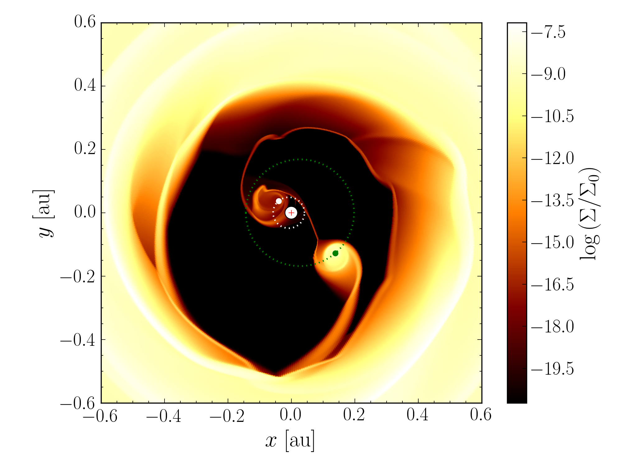
Figure 1: Two-dimensional plot of the inner disc of one of our locally isothermal Kepler-16 simulations where both orbits of the binary lie inside the computational domain. The logarithm of the surface density is colour-coded. The orbits of the primary and secondary are shown in white and green. The white inner region lies outside the computational domain; the red cross marks the centre of mass of the binary. A video of the simulation can be found online.

A snapshot of this simulation is plotted in Fig. 1. The logarithm of the surface density is colour-coded, while the orbits of the primary and secondary stars are shown in white and green. The red cross marks the centre of mass of the binary, which lies outside the computational domain. Figure 1 shows circumstellar discs around the binary components, as well as a complex gas flow through the gap onto the binary. Although including the binary orbit inside the computational would be desirable, it is at the moment not feasible for long-term simulations because of the strong time step restriction resulting from the small cell size at the inner boundary. This means that for simulations where the binary orbit is not included in the computational domain, the boundary condition at the inner radius has to allow for flow into the inner cavity, at least approximately. Two boundary conditions are usually used in circumbinary disc simulations: closed boundaries (Lines et al., 2015; Pierens & Nelson, 2013) and outflow boundaries (Kley & Haghighipour, 2014, 2015; Miranda et al., 2017).

Given the importance of the boundary condition at $R_{\mathrm{min}}$, we carried out dedicated simulations for a model adapted from Lines et al. (2015) and used an inner radius of $R_{\mathrm{min}}=$0.345\text{\,}\mathrm{a}\mathrm{u}$$, but otherwise it was identical to our standard model. We applied closed boundaries and open ones in order to examine their influence on the disc structure. We also varied different numerical parameters (resolution, radial grid spacing, integrator) for this simulation series.

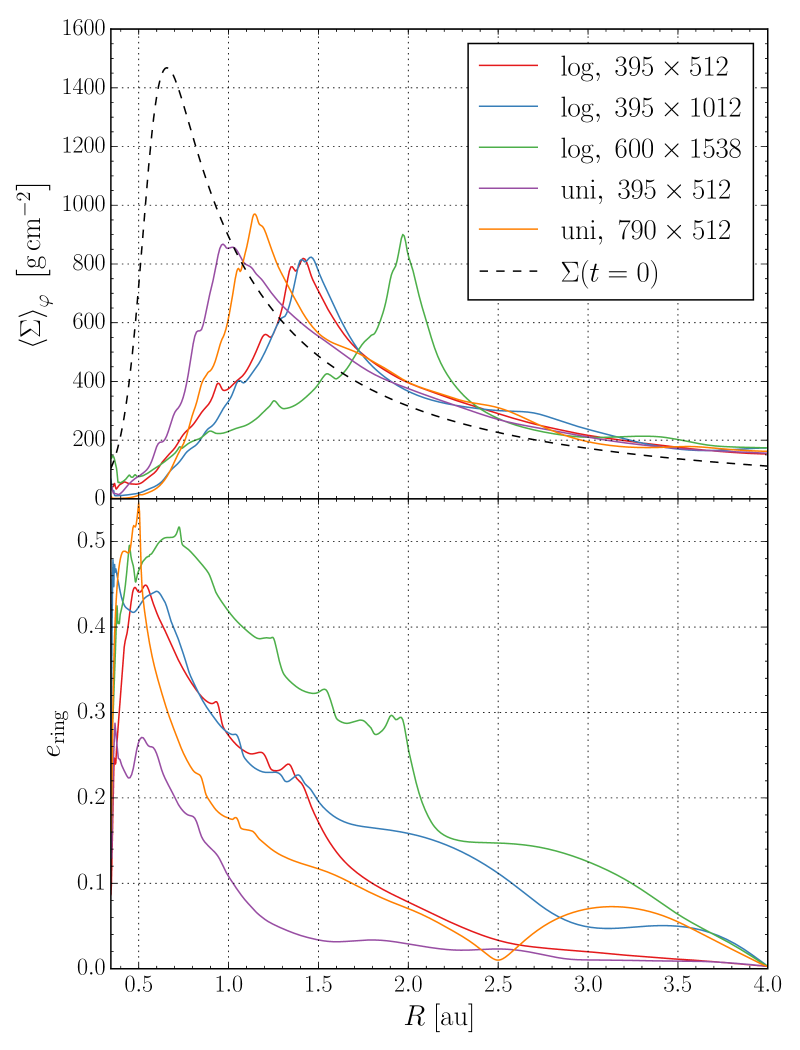
Figure 2: Azimuthally averaged surface density profiles (top) and radial disc eccentricity (bottom) for our Kepler-16 reference setup (using $R_{\mathrm{min}}=$0.345\text{\,}\mathrm{a}\mathrm{u}$$) with a closed inner boundary condition at $t=$16\,000$\,T_{\mathrm{bin}}$. Coloured solid lines show the results from simulations with different resolutions or different grid-spacing in the $R$-direction (logarithmic and uniform spacing). The initial density profile is also shown as a dashed black line. All simulations were performed with Pluto.

The top panel of Fig. 2 shows the azimuthally averaged density profiles for different grid resolutions and spacings after $16\,000$ binary orbits. All these simulations were performed with Pluto and a closed inner boundary. The strong dependence of the density distribution and inner gap size on the numerical setup stands out. This dependence on numerics is very surprising and not at all expected since the physical setup was identical in all these simulations and therefore the density profiles should all be similar and converge upon increasing resolution. Not only does the gap size show this strong dependence, but also the radial eccentricity distribution (bottom panel of Fig. 2). To examine this dependence further, which could in principle be the result of a bug in our code, we reran the identical physical setup with a different code, Rh2d. The results of these Rh2d simulations show the same strong numerical dependence as the Pluto results. In Fig. 3 the total disc eccentricity time evolution for the Rh2d simulations is plotted. Again, one would expect that different numerical parameters should produce approximately the same disc eccentricity, but our simulations show a radical change in the disc eccentricity if the numerical methods are slightly different.

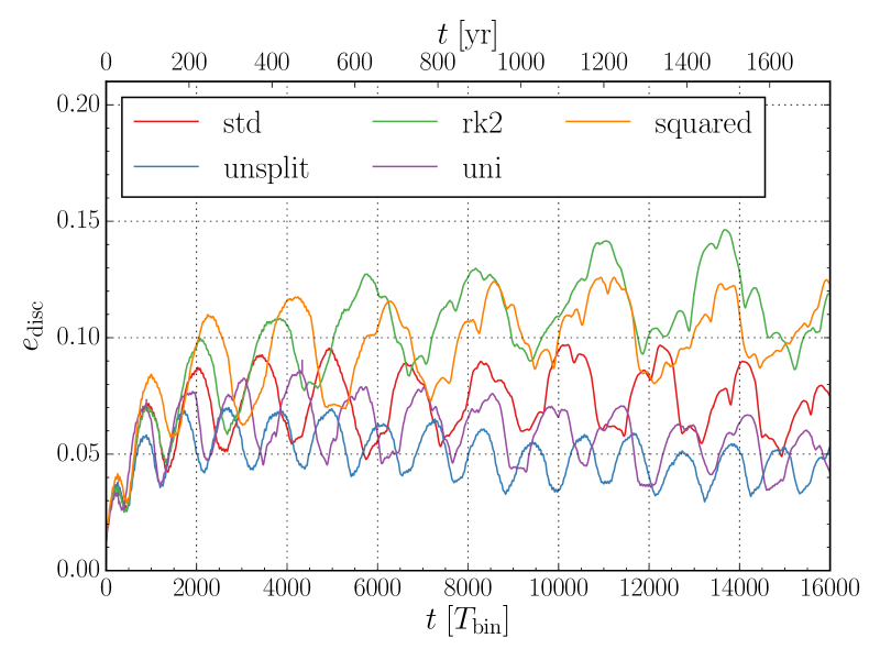
Figure 3: Time evolution of the total disc eccentricity for simulations of the standard model with closed inner boundary and $R_{\mathrm{min}}=$0.345\text{\,}\mathrm{a}\mathrm{u}$$. Different numerical parameters such as grid spacing, time integrator, and operator splitting have been used. The legend refers to: std standard integrator (operator and directional splitting), unsplit no directional splitting, Rk2 second-order RK time integrator, uni uniform grid, squared squared grid cells. All simulations were performed with Rh2d.

We note that using a viscous outflow condition where the radial velocity at $R_{\mathrm{min}}$ is fixed to $-\beta 3\nu/(2R)$ with $\beta=5$ (as suggested by Mutter et al. (2017)) resulted in the same dynamical behaviour as the closed boundary condition. The reason for this lies in the fact that the viscous speed is very low in comparison to the radial velocity induced by the perturbations of the central binary and hence there is little difference between a closed and a viscous boundary.

In contrast to the closed inner boundary simulations, simulations with a zero-gradient outflow inner boundary reach a quasi-steady state. For the open boundaries Pluto simulations with different numerical parameters produce very similar surface density and radial disc eccentricity profiles (Fig. 4) for different resolutions and grid spacings. Only the values for the uniform radial grid with a resolution of $395\times 512$ (purple line in Fig. 4) deviate. Here the resolution in the inner computational domain is not high enough, because a simulation with a higher resolution uniform grid ($790\times 512$, orange line in Fig. 4) produces approximately the same results as the simulations with a logarithmic radial grid spacing.

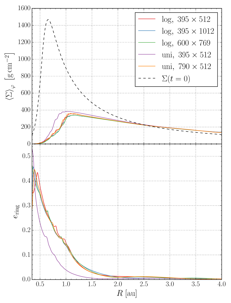
Figure 4: Azimuthally averaged surface density profiles (top) and radial disc eccentricity (bottom) for our reference setup ($R_{\mathrm{min}}=$0.345\text{\,}\mathrm{a}\mathrm{u}$$) with a zero-gradient outflow inner boundary condition after $16\,000$ binary orbits. Coloured solid lines show results from simulations with different resolutions or different grid-spacing in the $R$-direction (logarithmic and uniform spacing). The initial density profile is also shown as a dashed black line. All simulations were performed with Pluto.

We do not have a full explanation for this strong variability and non-convergence of the flow when using the closed inner boundary, but this result seems to imply that this problem is ill-posed. A closed inner boundary creates a closed cavity, which apparently implies in this case that the details of the flow depend sensitively on numerical diffusion as introduced by different spatial resolutions, time integrators, or codes. As a consequence, for circumbinary disc simulations a closed inner boundary is not recommended for two reasons. Firstly, it produces the described numerical instabilities and secondly, for physical reasons the inner boundary should be open because otherwise no material can flow into the inner region and be accreted by the stars. This is also indicated in Fig. 1 which shows mass flow through the inner gap, which cannot be modelled with a closed inner boundary.

4.2 Location of the inner radius

After determining that a zero gradient outflow condition is necessary, we use it now in all the following simulations and investigate in a second step the optimal location of $R_{\mathrm{min}}$. It should be placed in such a way that it simultaneously insures reliable results and computational efficiency. For the excitation of the disc eccentricity through the binary-disc interaction, non-linear mode coupling, and the 3:1 Lindblad resonance are important (Pierens & Nelson, 2013). Therefore, the location of the inner boundary is an important parameter and $R_{\mathrm{min}}$ should be chosen such that all major mean-motion resonances between the disc and the binary lie inside the computational domain. To investigate the influence of the inner boundary position, we set up simulations with an inner radius from $R_{\mathrm{min}}=$0.12\text{\,}\mathrm{a}\mathrm{u}$$ to $R_{\mathrm{min}}=$0.5\text{\,}\mathrm{a}\mathrm{u}$$ for the standard system parameter as noted in Table 2.

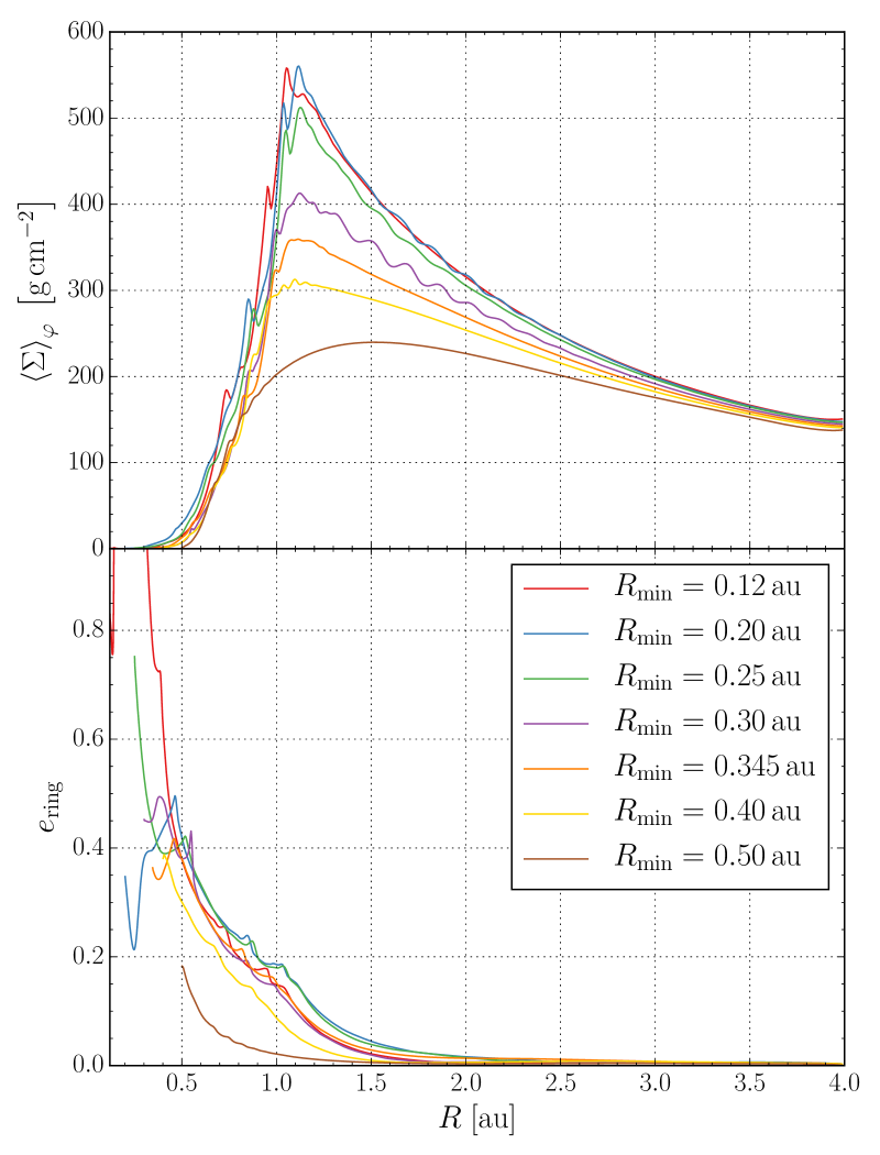
Figure 5: Influence of different inner radii on the disc structure for simulations with a zero-gradient outflow inner boundary condition. Top: Azimuthally averaged surface density profiles after $16\,000$ binary orbits. Bottom: Radial disc eccentricity distribution at the same time.

Fig. 5 shows the results of these simulations. Displayed are the azimuthally averaged surface density and the radial disc eccentricity distribution after $16\,000$ binary orbits. In agreement with Kley & Haghighipour (2014), we find that the radial disc eccentricity does not depend much on the location of the inner radius and remains low in the outer disc ($R>$2\text{\,}\mathrm{a}\mathrm{u}$$). Only for a large inner radius of $R_{\mathrm{min}}=$0.5\text{\,}\mathrm{a}\mathrm{u}$$ do we observe almost no disc eccentricity growth (brown line in Fig. 5). In this case the 3:1 Lindblad resonance ($R_{3:1}=$0.46\text{\,}\mathrm{a}\mathrm{u}$$) lies outside the computational domain, confirming the conclusion from Pierens & Nelson (2013) about the importance of the 3:1 Lindblad resonance for the disc eccentricity growth. The variation of the radial disc eccentricity for inner radii smaller than $0.3\text{\,}\mathrm{a}\mathrm{u}$ occurs because the precessing discs are in different phases after $16\,000$ binary orbits. Contrary to the eccentricity distribution, the azimuthally averaged surface density shows a stronger dependence on the inner radius. As seen in the top panel of Fig. 5, the maximum of the surface density increases monotonically as the location of the inner boundary decreases because a smaller inner radius means also that the ?area? where material can leave the computational domain decreases. For inner radii smaller than $R_{\mathrm{min}}\leq$0.25\text{\,}\mathrm{a}\mathrm{u}$$ the change in the maximum surface density becomes very low upon further reduction of $R_{\mathrm{min}}$. This implies that for too large $R_{\mathrm{min}}$ there is too much mass leaving the domain and it has to chosen small enough to capture all dynamics. Although the maximum value of the surface density increases, the position of the maximum does not depend on the inner radius and remains at approximately $R=$1.1\text{\,}\mathrm{a}\mathrm{u}$$ as long as the 3:1 Lindblad resonance lies inside the computational domain. Furthermore, we find that the slope of the surface density profile at the gap’s edge does not depend on the location of the inner boundary. These results are in contrast to Mutter et al. (2017) who find a stronger dependence of the density profile on the location of the inner radius. However, their results may be a consequence of the viscous outflow condition used.

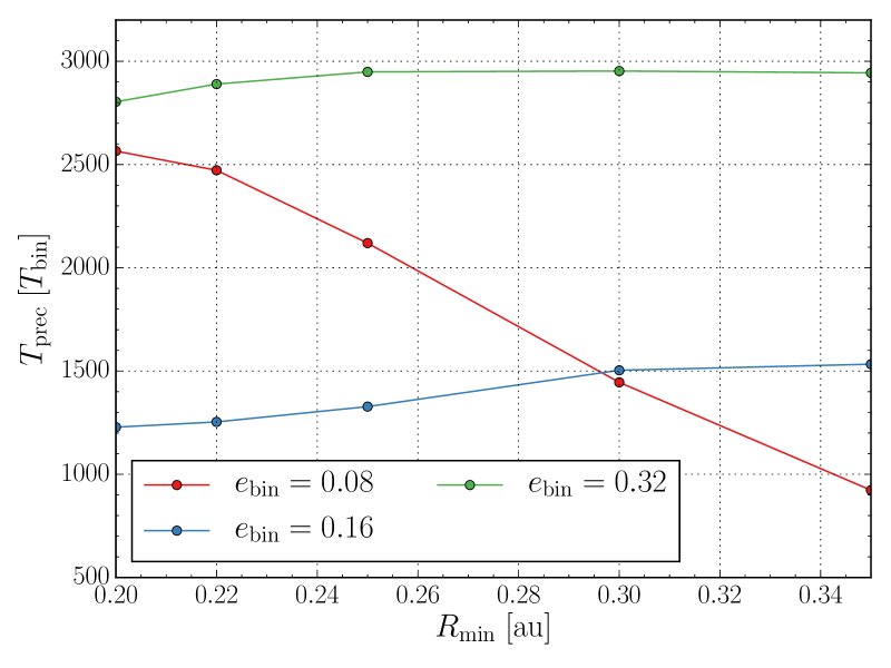
Figure 6: Variation of precession period of the inner gap of the disc for varying inner radii, $R_{\mathrm{min}}$, and different binary eccentricities, $e_{\mathrm{bin}}$.

As is discussed below, the disc becomes eccentric with a slow precession that depends on the binary eccentricity, $e_{\mathrm{bin}}$. To explore how the location of the inner radius affects the disc dynamics, we ran additional simulations with varying $R_{\mathrm{min}}$ for different $e_{\mathrm{bin}}$. We chose $e_{\mathrm{bin}}=0.08$ and $e_{\mathrm{bin}}=0.32$ in addition to the Kepler-16 value of $e_{\mathrm{bin}}=0.16$, which lies near the bifurcation point, $e_{\mathrm{crit}}$. Fig. 6 shows the precession period of the inner gap for varying inner radii and three different binary eccentricities, where the blue curve refers to the model shown above with $e_{\mathrm{bin}}=0.16$. For a higher binary eccentricity of $e_{\mathrm{bin}}=0.32$ (green curve in Fig. 6 and on the upper branch of the bifurcation diagram) the disc dynamics seems to be captured well even for higher values of $R_{\mathrm{min}}$. Only for values lower than $R_{\mathrm{min}}=$0.22\text{\,}\mathrm{a}\mathrm{u}$$ are deviations seen. The simulation with $R_{\mathrm{min}}=$0.20\text{\,}\mathrm{a}\mathrm{u}$$ was more unstable, probably because the secondary moved in and out of the computational domain on its orbit. On the lower branch of the bifurcation diagram the convergence with decreasing $R_{\mathrm{min}}$ is slower as indicated by the case $e_{\mathrm{bin}}=0.08$ (red curve in Fig. 6). Here, an inner radius of $R_{\mathrm{bin}}=a_{\mathrm{bin}}$ or even slightly lower may be needed. One explanation for this behaviour is that on the lower branch (for low $e_{\mathrm{bin}}$) the inner gap is smaller but nevertheless quite eccentric such that the disc is influenced more by the location of the inner boundary. The convergence of the results for smaller inner radii is also visible in the azimuthally averaged surface density and radial eccentricity profiles for $e_{\mathrm{bin}}=0.08$ and $e_{\mathrm{bin}}=0.32$ displayed in Fig. 7.

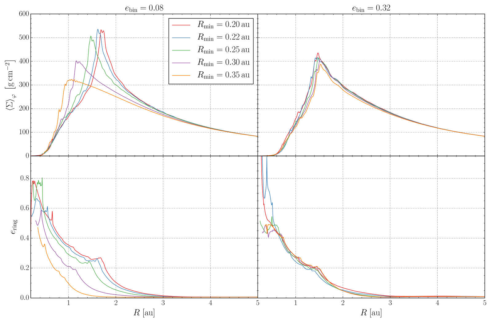
Figure 7: Influence of different inner radii and binary eccentricities on the disc structure for simulations with a zero-gradient outflow inner boundary condition. Top: Azimuthally averaged surface density profiles after $16\,000$ binary orbits. Bottom: Radial disc eccentricity distribution at the same time. Left: $e_{\mathrm{bin}}=0.08$. Right: $e_{\mathrm{bin}}=0.32$

In summary, from the results shown in Figs. 5, 6, and 7 we can conclude that to model the circumbinary disc properly, the inner radius should correspond to $R_{\mathrm{min}}\approx a_{\mathrm{bin}}$. This should be used in combination with a zero-gradient outflow (hereafter just outflow) condition. Since a smaller inner boundary increases the number of radial cells and imposes a stricter condition on the time step, long-term simulations with a small inner radius are very expensive. As a compromise to make long-term simulations possible, we have chosen in all simulations below an inner radius of $R_{\mathrm{min}}=$0.25\text{\,}\mathrm{a}\mathrm{u}$$.

4.3 Location of the outer radius

While investigating the numerical conditions at the inner radius, we used an outer radius of $R_{\mathrm{max}}=$4.0\text{\,}\mathrm{a}\mathrm{u}$$ and assumed that this value is high enough, so that the outer boundary would not interfere with the dynamical behaviour of the inner disc. During our study of different binary and disc parameters, we found that in some cases this assumption is not true. Especially for binary eccentricities greater than $0.32$, reflections from the outer boundary interfered with the complex inner disc structure. Therefore, we increased the outer radius of all the following simulations to $R_{\mathrm{max}}=$15.4\text{\,}\mathrm{a}\mathrm{u}$=$70$\,a_{\mathrm{bin}}$, a value used by Miranda et al. (2017). In order to keep the same spatial resolution as before we also increased the resolution to $$762$\times$582$$ cells. This ensures that in the radial direction we still have $512$ grid cells between $0.25\text{\,}\mathrm{a}\mathrm{u}$ and $4.0\text{\,}\mathrm{a}\mathrm{u}$. To save computational time it is also possible to use a smaller outer radius ($R_{\mathrm{max}}\approx 40\,a_{\mathrm{bin}}$) with a damping zone where the density and radial velocity are relaxed to their initial value. A detailed description of the implementation of such a damping zone can be found in de Val-Borro et al. (2006).

Hence, for our subsequent simulations we use from now on the numerical setup quoted in Table 2, unless otherwise stated. To study the dependence on different physical parameter we start from the standard values of the Kepler-16 system in Table 2 and vary individual parameter separately.

Table 2: Setup for our reference model.

Numerical parameters
$R_{\mathrm{min}}$	$0.25\text{\,}\mathrm{a}\mathrm{u}$
$R_{\mathrm{max}}$	$15.4\text{\,}\mathrm{a}\mathrm{u}$
Resolution	$762\times 582$
Inner boundary	Outflow
Binary parameters
$a_{\mathrm{bin}}$	$0.22\text{\,}\mathrm{a}\mathrm{u}$
$e_{\mathrm{bin}}$	$0.16$
$q_{\mathrm{bin}}$	$0.29$
Disc parameters
$h$	$0.05$
$\alpha$	$0.01$

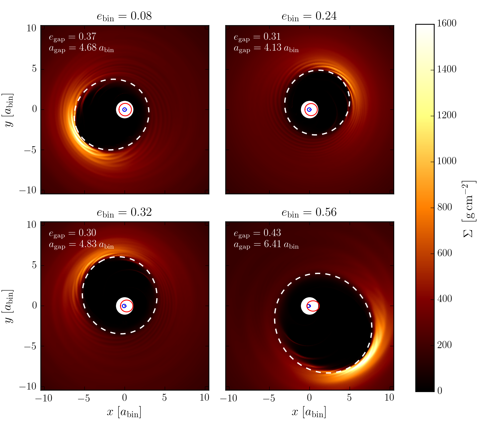
Figure 8: Structure of the inner disc for different binary eccentricities after $16\,000$ binary orbits. The surface density is colour-coded in cgs-units. The orbits of the primary and secondary around the centre of mass (central point) are shown in blue and red. The white dashed lines represent approximate ellipses fitted to match the extension of the inner gap (see explanation in text). Videos of these simulations can be found online.

5 Variation of binary parameters

In this section we study the influence of the central binary parameter specifically its orbital eccentricity and mass ratio on the disc structure. Throughout this section we use a disc aspect ratio of $h=0.05$ and a viscosity $\alpha=0.01$. For the inner radius and the inner boundary condition we use the results from the previous section and apply the outflow condition at $R_{\mathrm{min}}$ (see also Table 2). All the results in this section were obtained with Pluto, but comparison simulations using Rh2d show very similar behaviour (see Fig. 23).

5.1 Dynamics of the inner cavity

Before discussing in detail the impact of varying $e_{\mathrm{bin}}$ and $q_{\mathrm{bin}}$, we comment first on the general dynamical behaviour of the inner disc. Fig. 8 shows snapshots of the inner disc after $16\,000$ binary orbits for different binary eccentricities. As seen in several other studies (as mentioned in the introduction) we find that the inner disc becomes eccentric and shows a coherent slow precession. In the figure we overplot ellipses (white dashed lines) that are approximate fits to the central inner cavity, where the semi-major axis ($a_{\textrm{gap}}$) and eccentricity ($e_{\textrm{gap}}$) are indicated. To calculate these parameters we assumed first that the focus of the gap-ellipse is the centre of mass of the binary. We then calculated from our data the coordinates $(R_{\Sigma\mathrm{max}},\varphi_{\Sigma\mathrm{max}})$ of the cell with the highest surface density value, which defines the direction to the gap’s apocentre. We defined the apastron of the gap $R_{\mathrm{apa}}$ as the minimum radius along the line $(R,\varphi_{\Sigma\mathrm{max}})$ which fulfils the condition

$$\Sigma(R,\varphi_{\Sigma\mathrm{max}})\geq 0.1\cdot\Sigma(R_{\Sigma\mathrm{max}},\varphi_{\Sigma\mathrm{max}})\,.$$ (21)

The periastron of the gap $R_{\mathrm{peri}}$ is defined analogously as the minimum radius along the line $(R,\varphi_{\Sigma\mathrm{max}}+\pi)$ in the opposite direction which fulfils

$$\Sigma(R,\varphi_{\Sigma\mathrm{max}}+\pi)\geq 0.1\cdot\Sigma(R_{\Sigma\mathrm{max}},\varphi_{\Sigma\mathrm{max}})\,.$$ (22)

Using the apastron and periastron of the gap as defined above, the eccentricity and semi-major axis of the gap are given by

$$a_{\mathrm{gap}} =0.5\left(R_{\mathrm{apa}}+R_{\mathrm{peri}}\right)\,,$$ (23)

$$e_{\mathrm{gap}} =R_{\mathrm{apa}}/a_{\mathrm{gap}}-1\,.$$ (24)

As shown in Fig. 8 this purely geometrical construction matches the shape of the central cavity very well. Even though the overall disc behaviour shows a rather smooth slow precession, the dynamical action of the central binary is visible as spiral waves near the gap’s edges, most clearly seen in the first and last panel. We prepared some online videos to visualise the dynamical behaviour of the inner disc.

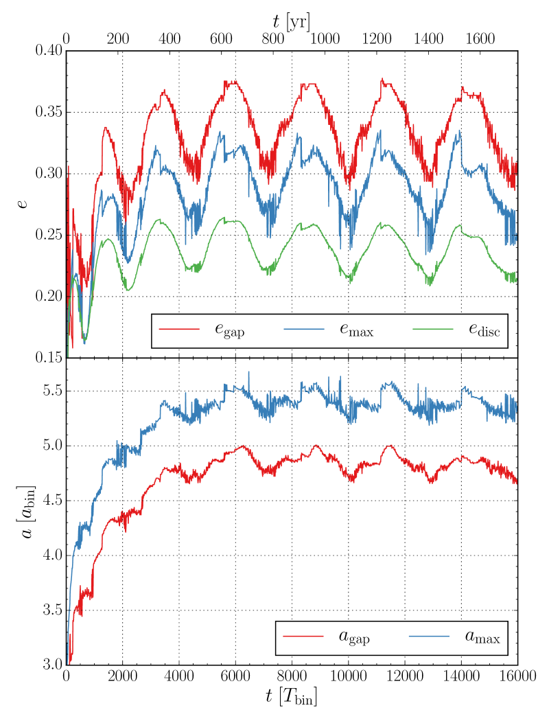
Figure 9: Evolution of gap eccentricity (top) and semi-major axis (bottom) for a binary with $e_{\mathrm{bin}}=0.30$. Shown are different measurements for the disc eccentricity. The red lines ($e_{\mathrm{gap}}$ and $a_{\mathrm{gap}}$) show the eccentricity and semi-major axis of the geometrically fitted ellipses, see Fig. 8. The blue lines ($e_{\mathrm{max}}$ and $a_{\mathrm{max}}$) show the eccentricity and semi-major axis of the cell with the maximum surface density. The green curve shows the averaged eccentricity of the inner disc. Since the gap size varies with time we use $R_{2}=R_{\Sigma\mathrm{max}}$ in eq. (18) to calculate the inner disc eccentricity.

An alternative way to characterise the disc gap dynamically is by using the orbital elements ($e_{\mathrm{max}},a_{\mathrm{max}}$) of the cell with the maximum surface density. These orbital elements can be calculated with equation (15) and the vis-viva equation

$$a=\left(\frac{2}{R}-\frac{\bm{\mathrm{u}}^{2}}{GM_{\mathrm{bin}}}\right)^{-1}\,.$$ (25)

The time evolution of these gap characteristics are plotted in Fig. 9. The gap’s size and eccentricity show in phase oscillatory behaviour with a larger amplitude in the eccentricity variations. The period of the oscillation is identical to the precession period of the disc. Clearly, the extension of the gap always lies inside of the location of maximum density $a_{\mathrm{gap}}<a_{\mathrm{max}}$, but for the eccentricities the ordering is not so clear. The radial variations of the disc eccentricity as shown in Figs. 4 and 5 indicate that the inner regions of the disc typically have a higher eccentricity. In Fig. 9 $e_{\mathrm{disc}}$ is lowest because it is weighted with the density which is very low in the inner disc regions. The eccentricity for the gap $e_{\mathrm{gap}}$ stems from a geometric fit to the very inner disc regions and is the highest. Inside the maximum density and even slightly beyond that radius the disc precesses coherently in the sense that the pericentres estimated at different radii are aligned. The data show further that when the disc eccentricity is highest the disc is fully aligned with the orbit of the secondary star, i.e. the pericentre of disc and binary lie in the same direction (see also Appendix A).

5.2 Binary eccentricity

For simulations in this section we fixed $q_{\mathrm{bin}}=0.29$ and varied $e_{\mathrm{bin}}$ from $0.0$ to $0.64$. The binary eccentricity strongly influences the size of the gap as well as the disc precession period of the inner disc.

In Fig. 10 the azimuthally averaged surface density profiles are shown for the various $e_{\mathrm{bin}}$ at $16\,000$ binary orbits. In all cases there is a pronounced density maximum visible which is the strongest for the circular binary with $e_{\mathrm{bin}}=0$ (red curve). The position of the peak varies systematically with binary eccentricity. Increasing $e_{\mathrm{bin}}$ from zero to higher values the peak shifts inward. Not only does the gap size decrease, but the maximum surface density also drops with increasing $e_{\mathrm{bin}}$ until a minimum at $e_{\mathrm{bin}}=0.18$ is reached. Increasing $e_{\mathrm{bin}}$ further causes the density peak to move outward again, whereas the maximum surface density stays roughly constant for higher binary eccentricities.

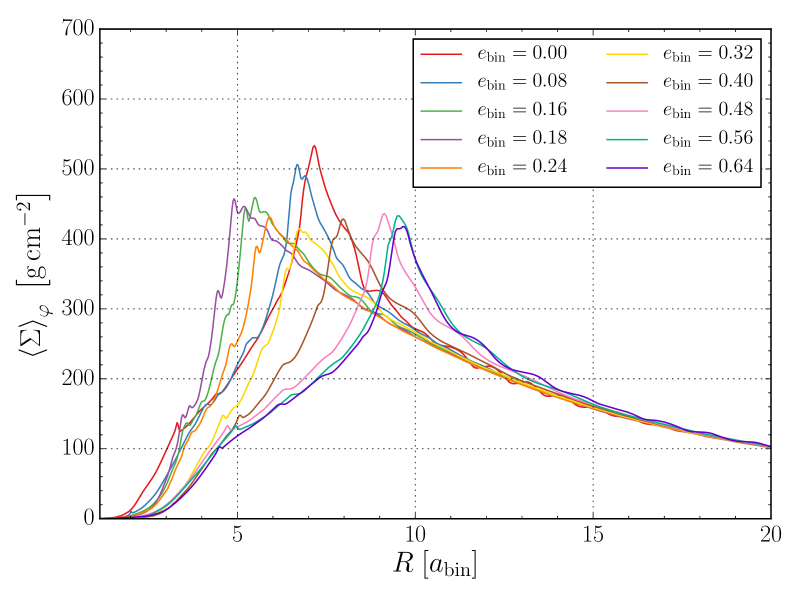
Figure 10: Azimuthally averaged density profiles for varying binary eccentricities after $16\,000$ binary orbits. For clarity we only show selected results from the simulated parameter space.

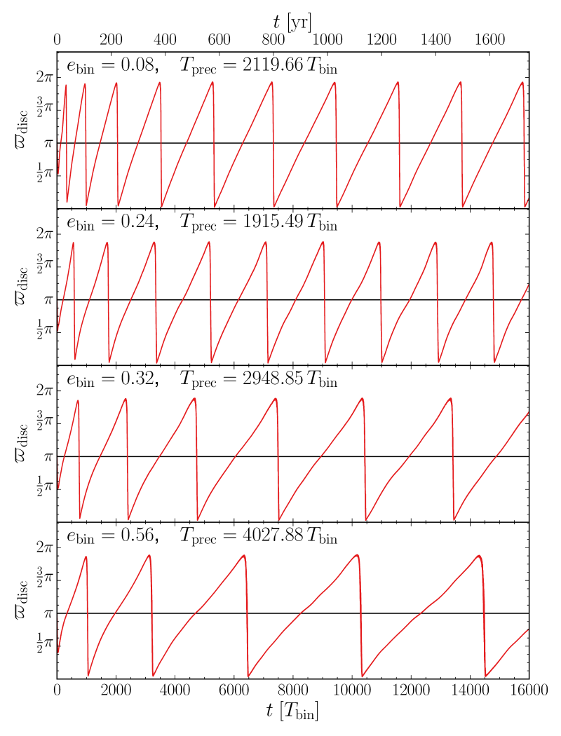
Figure 11: Disc longitude of periastron for different binary eccentricities for the inner disc $R<1.0\,\mathrm{au}$. For all cases a clear prograde precession of the inner disc is visible and the precession period, $T_{\mathrm{prec}}$, is indicated in the legend.

As mentioned above, the eccentric disc precesses slowly and in Fig. 11 the longitude of the inner disc’s pericentre is shown versus time over $16\,000$ binary orbits. The disc displays a slow prograde precession with inferred period of several thousand binary orbits. For the measurement of the precession period we discarded the first $6000$ binary orbits since plots of the longitude of periastron show that during this time span the precession period is not constant yet (see Fig. 11). The period is then calculated by averaging over at least two full periods. To be able to average over two periods, models with a very long $T_{\mathrm{prec}}$ (e.g. $e_{\mathrm{bin}}=0.64$) were simulated for more than $16\,000$ binary orbits.

Fig. 12 summarises the results from simulations with varying binary eccentricities.

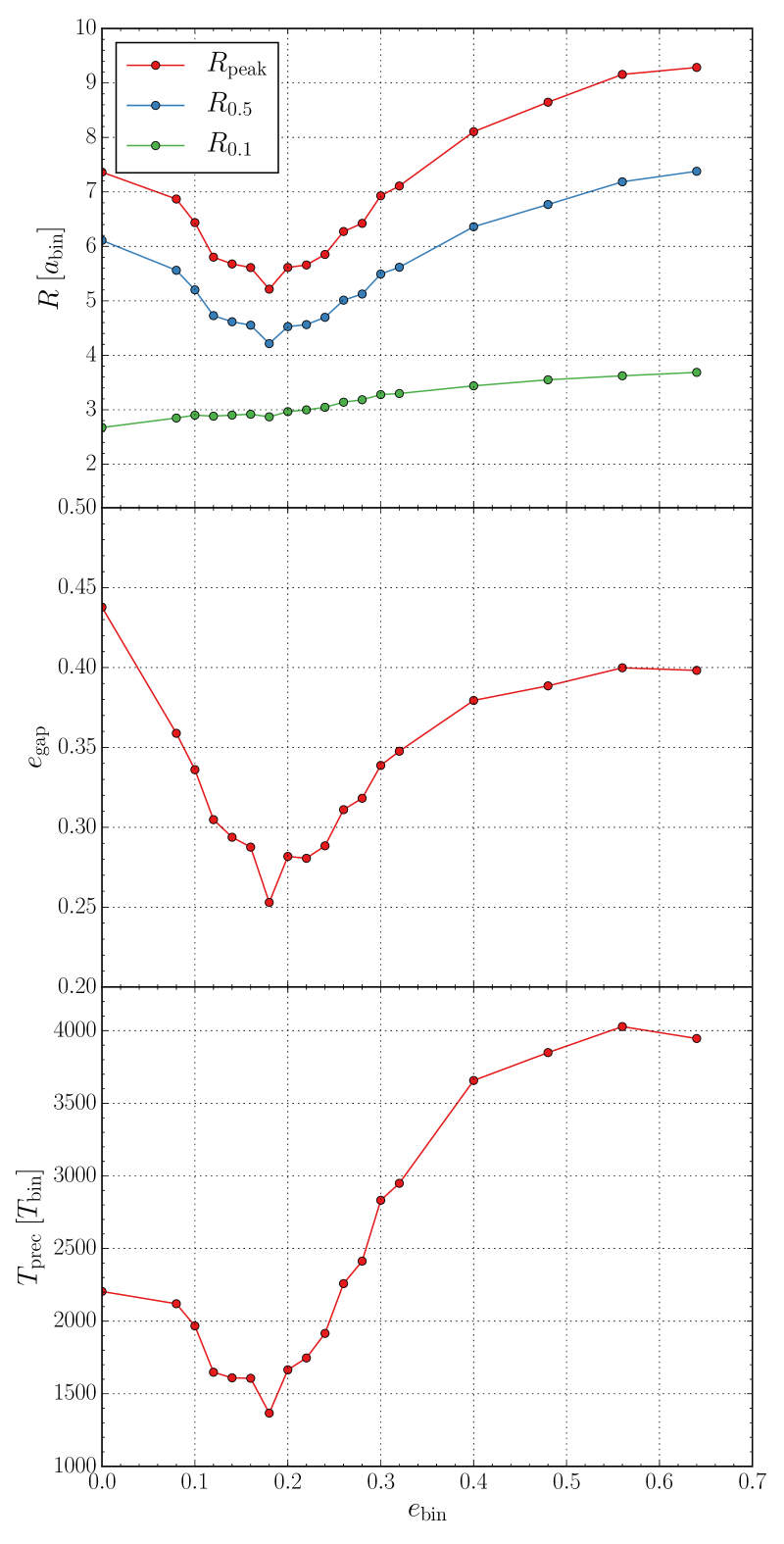
Figure 12: Influence of different binary eccentricities on gap size, gap eccentricty, and precession rate. Top: Different measures of the gap size are shown, averaged over several thousand binary orbits. The value $R_{\mathrm{peak}}$ refers to the location of maximum of the averaged surface density (see Fig. 10), while $R_{\mathrm{0.5}}$ and $R_{\mathrm{0.1}}$ refer to density drops of 50 and 10 percent of the maximum value. Middle: Eccentricity of the gap. Bottom: Precession period of the disc gap.

The top panel of Fig. 12 shows different measures for the gap size for varying binary eccentricities. In addition to the radial position where the azimuthally averaged surface density reaches its maximum ($R_{\mathrm{peak}}$), we plot the positions where the density drops to 50 and 10 percent of its maximum value ($R_{\mathrm{0.5}}$ and $R_{\mathrm{0.1}}$). The value $R_{\mathrm{0.5}}$ was used by Kley & Haghighipour (2014) as a measure for the gap size, whereas Miranda et al. (2017) used $R_{\mathrm{0.1}}$ and Mutter et al. (2017) $R_{\mathrm{peak}}$. Starting from a non-eccentric binary the curves for $R_{\mathrm{peak}}$ and $R_{\mathrm{0.5}}$ decrease with increasing binary eccentricity. For $e_{\mathrm{bin}}\approx 0.18$ the gap size reaches a minimum and then increases again for higher binary eccentricities. In agreement with Miranda et al. (2017) we see an almost monotonic increase of $R_{\mathrm{0.1}}$ for increasing binary eccentricities. The gap size, $a_{\mathrm{gap}}$, correlates well with $R_{\mathrm{0.5}}$ and is always about 14% smaller.

The middle panel of Fig. 12 shows the eccentricity of the inner cavity, calculated with the method described in Sec. 5.1. The disc eccentricity also changes systematically with $e_{\mathrm{bin}}$. For circular binaries it reaches $e_{\mathrm{gap}}\approx 0.44$, and then it drops down to about 0.25 for the turning point $e_{\mathrm{bin}}=0.18$, and increases again reaching $e_{\mathrm{gap}}\approx 0.4$ for the highest $e_{\mathrm{bin}}=0.64$. Hence, for nearly circular binaries $e_{\mathrm{gap}}$ can be higher than for more eccentric binaries. A similar variation of the disc’s eccentricity and precession rate with binary eccentricity has been noticed by Fleming & Quinn (2017) who attribute this to the possible excitation of higher order resonances for higher disc eccentricities.

The bottom panel of Fig. 12 shows the precession period of the inner disc ($R<$1\text{\,}\mathrm{a}\mathrm{u}$$) for different binary eccentricities. The curve for the precession period shows a similar behaviour to the upper curves for the gap size. To investigate further the correlation of the gap size (here represented by $R_{\mathrm{0.5}}$) and the precession period, we show in Fig. 13 the two quantities plotted against each other.

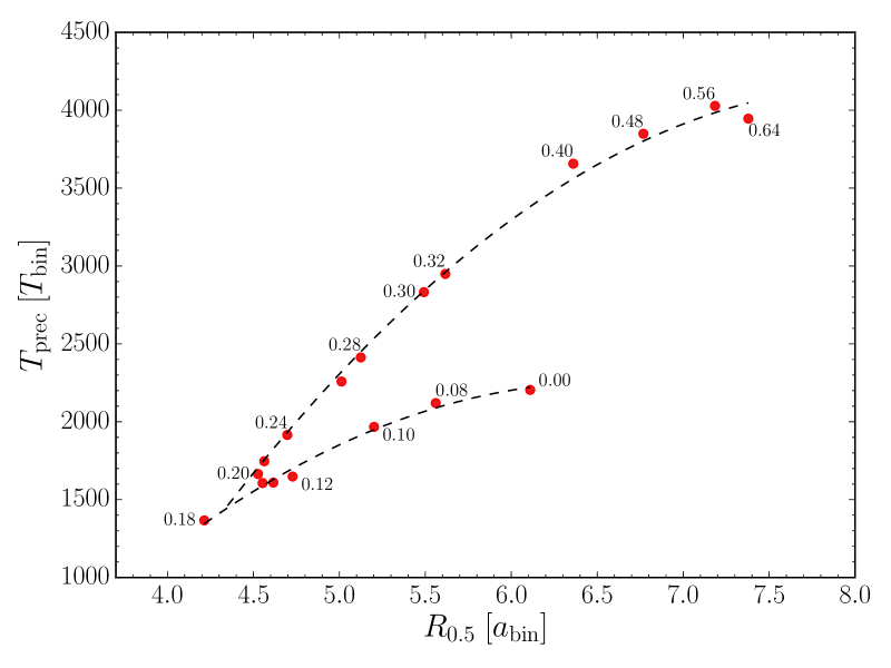
Figure 13: Precession rate of the gap plotted against the radius where the azimuthally averaged surface density drops to 50 percent of its maximum value ($R_{\mathrm{0.5}}$), averaged over several thousand binary orbits. Different dots correspond to different binary eccentricities. The dashed lines are not fit curves but are just drawn to guide the eye.

Two branches can be seen as indicated by the dashed curves. One starts at $e_{\mathrm{bin}}=0.0$ and goes to $e_{\mathrm{bin}}=0.18$ where the gap size and precession period decrease with increasing binary eccentricities, and the other branch starts at the minimum at $e_{\mathrm{bin}}=0.18$ where both gap properties increase again with increasing binary eccentricities. These two branches may indicate two different physical processes that are responsible for the creation of the eccentric inner gap and show the direct correlation between precession period and gap size.

In our simulations all discs became eccentric and showed a prograde precession, and we did not find any indication for ?stand still? discs that are eccentric but without any precession. In contrast, Miranda et al. (2017) find for their disc setup ($h=0.1,\alpha=0.1$) that the disc does not precess for binary eccentricities between $0.2$ and $0.4$. We do not find this behaviour for our disc models, but note that we use a disc with a lower aspect ratio and a lower $\alpha$-value. To investigate this further we set up a simulation with the same numerical parameters as Miranda et al. (2017) and used a physical setup where they did not observe a precession of the disc ($q_{\mathrm{bin}}=1.0$, $e_{\mathrm{bin}}=0.4$, $h=0.1$, and $\alpha=0.1$). We carried out two simulations, one with an inner radius of $R_{\mathrm{min}}=(1+e_{\mathrm{bin}})a_{\mathrm{bin}}$ and one with an inner radius of $R_{\mathrm{min}}=$1.136$\,a_{\mathrm{bin}}$. The first radius was used by Miranda et al. (2017) and in this case we also observe no precession of the disc. The second radius corresponds to $R_{\mathrm{min}}=$0.25\text{\,}\mathrm{a}\mathrm{u}$$, which is the radius we established in Sect. 4.2 as the optimum location of the inner boundary. In the case with the smaller inner radius we observe a clear precession of the inner disc (Fig. 14) with a relatively short precession period $T_{\mathrm{prec}}$ as expected for high viscosity and high $h$ (see below). This is another indication of the necessity of choosing $R_{\mathrm{min}}$ sufficiently small to capture all effects properly.

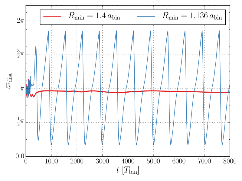
Figure 14: Disc longitude of periastron for different inner radii of the computational domain. The red line shows results from a simulation with the Miranda et al. (2017) setup where no precession of the disc is observable. The blue line shows results from the same physical setup but with a smaller inner disc radius. In this case a clear precession of the inner disc is visible.

5.3 Binary mass ratio

In this section we study the influence of the binary mass ratio. We carried out simulations with a mass ratio from $q_{\mathrm{bin}}=0.1$ to $q_{\mathrm{bin}}=1.0$; all other parameters were set according to Table 2. Fig. 15 shows the azimuthally averaged density profiles for varying binary mass ratios.

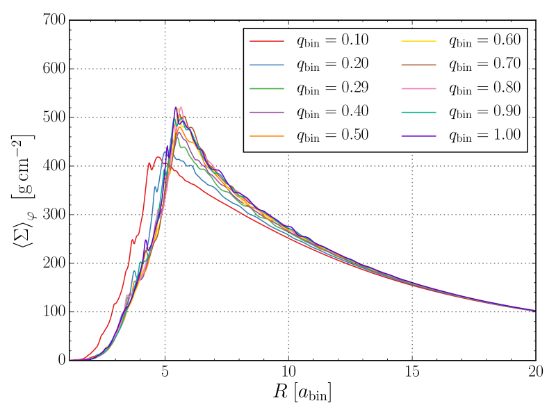
Figure 15: Azimuthally averaged density profiles for varying binary mass ratio after $16\,000$ binary orbits.

The density profiles do not show such a strong variation as in simulations with varying binary eccentricities. Only the density profiles of the two lowest simulated mass ratios $q_{\mathrm{bin}}=0.1$ and $q_{\mathrm{bin}}=0.2$ differ significantly from the other profiles. For these models the position of the peak surface density is closer to the binary and the maximum surface density roughly 20 percent lower. The different gap size measures, introduced in the previous section, are shown in the top panel of Fig. 16. In general, the variations of all three gap-size indicators with mass ratio $q_{\mathrm{bin}}$ are relatively weak. All three gap size measurements remain nearly constant for mass ratios greater than $0.3$. Since the density profiles do not show a significant variation this is not surprising. At the same time the size and eccentricity of the gap do not vary significantly and lie in the range $a_{\mathrm{gap}}\approx 4\,a_{\mathrm{bin}}$ and $e_{\mathrm{gap}}\approx 0.27$. Overall, compared to simulations with varying binary eccentricity the binary mass ratio does not have such a strong influence on the inner disc structure for $q_{\mathrm{bin}}\gtrsim 0.3$.

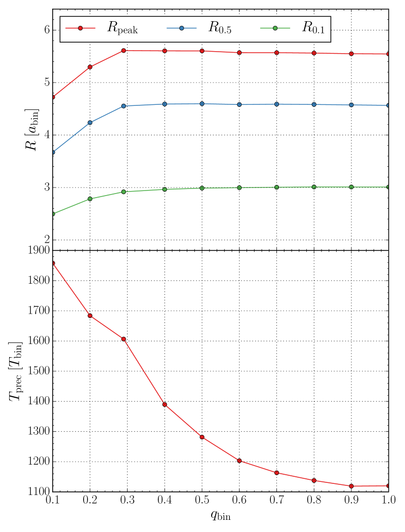
Figure 16: Influence of different binary mass ratios on gap size and precession rate. Top: Different measures of the gap size averaged over several thousand binary orbits. Bottom: Precession period of the disc gap.

In contrast, the precession period of the inner disc shows a far stronger dependence on the binary mass ratio than the gap size (bottom panel of Fig. 16). Discs around binaries with a higher mass ratio have a lower precession period than discs around binaries with a low mass ratio. This dependence can be understood in terms of free particle orbits around a binary star that also display a reduction of the precession period with increasing $q$, as we discuss in more detail in Appendix B.

6 Variation of disc parameters

In this section we explore the influence of discs parameters, namely the aspect ratio and the alpha viscosity, on the inner disc structure. We use the Kepler-16 values for the binary and our standard numerical setup (Table 2).

While performing the simulations for this paper we observed that models with low pressure (low $H/R$) and high viscosity (high $\alpha$) seem to be very challenging for the Riemann-Code Pluto. As a consequence we also present in this section results using the Upwind-Code Rh2d. As discussed in Appendix A, the two codes produce results in very good agreement with each other for our standard model. For other parameters they do not necessarily produce results with such good agreement, but the simulation results from both codes always show the same trend. Therefore, we decided to mix simulation results from Pluto and Rh2d to cover a broader parameter range.

6.1 Disc aspect ratio

First we varied the disc aspect ratio $h$ from $0.03$ to $0.1$. Our simulation results show a decreasing gap size for higher aspect ratios (Fig. 17). The gaps precession period is again directly correlated to the gap size, an observation we have already seen for different binary eccentricities.

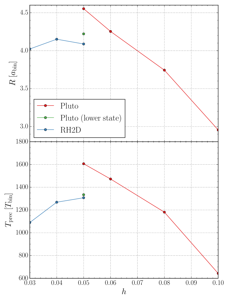
Figure 17: Influence of different disc aspect ratios on gap size and precession rate. Top: Radius where the density drops to 50 percent of its maximum value averaged over several thousand binary orbits. Since results from two different codes are shown, we omit the two other measurements for the gap size presented in previous sections. Bottom: Precession period of the disc gap. For $e_{\mathrm{bin}}\approx 0.16$ we observed that Pluto simulations can switch between two states, an upper state (red) and a lower state (green). For RH2D simulations we only observed the lower state (blue). This is discussed in more detail in Appendix A.

In general, a drop in $T_{\mathrm{prec}}$ with higher $h$ is expected because an increase in pressure will tend to reduce the gap size, which will in turn lead to a faster precession. This trend is indeed observed in our simulations for higher $h$. For simulations with $h<0.05$ we observed a decrease in gap size and precession period. The drop in $T_{\mathrm{prec}}$ with lower values of $h$ may be partly due to the lack of numerical resolution and partly to the lack of pressure support, which may no longer allows for coherent disc precession.

6.2 Alpha viscosity

In this section we discuss the influence of the magnitude of viscosity on the disc structure and therefore set up simulations with different viscosity coefficients ranging from $\alpha=0.001$ to $\alpha=0.1$. We then analysed the structure and behaviour of the inner cavity as before. The results are summarised in Fig. 18. A clear trend is visible for the gap size and for the precession period of the gap. For higher viscosities the gap size shrinks and the precession period decreases. Again, we see the direct correlation of gap size and precession rate, as already observed for aspect ratio and binary eccentricity variations. The decrease in the disc’s gap size can be explained: for higher $\alpha$ values the viscous spreading of the disc increases. This viscous spreading counteracts the gravitational torques of the binary, which are responsible for the gap creation.

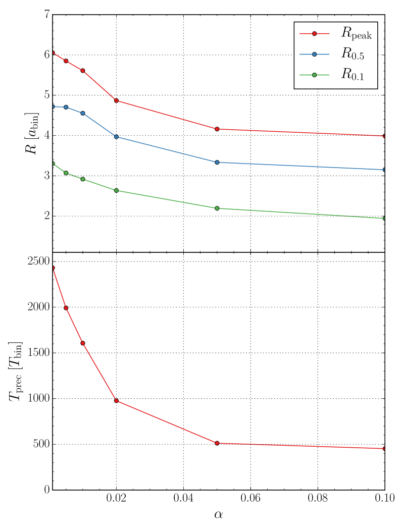
Figure 18: Influence of different disc viscosities on gap size and precession rate. Top: Different measures of the gap size averaged over several thousand binary orbits. Bottom: Precession period of the disc gap.

7 Summary and discussion

Using two-dimensional hydrodynamical simulations, we studied the structure of circumbinary discs for different numerical and physical parameters. Since these simulations are, from a numerical point of view, not trivial and often it is not easy to distinguish physical features and numerical artefacts, we checked our results with three different numerical codes. In the following we summarise the most important results from our simulations with different numerical and physical parameters.

Concerning the numerical treatment the most crucial issue with simulations using grid codes in cylindrical coordinates is the treatment of the inner boundary condition. As there has been some discussion in the literature about this issue (Pierens & Nelson, 2013; Kley & Haghighipour, 2014; Lines et al., 2015; Miranda et al., 2017; Mutter et al., 2017), we decided to perform a careful study of the location of the inner boundary and the conditions on the hydrodynamical variables at $R_{\mathrm{min}}$. Our results can be summarised as follows:

• Inner boundary condition. Since there was no agreement on which type of inner boundary condition should be used for circumbinary disc simulations, especially if closed or open boundary conditions should be used, we investigated the influence of the inner boundary condition through dedicated simulations with two different codes. We observed that closed boundaries can lead to numerical instabilities for all codes used in our comparison and no convergence to a unique solution could be found. The use of a viscous outflow condition where the velocity is set to the mean viscous disc speed produced very similar results to the closed boundary because the viscous speed is very low in comparison to the velocities induced by the dynamical action of the binary stars. Open inner boundaries, on the other hand, lead to numerically stable results and are also, from a physical point of view, more logical because material can flow onto the binary and be accreted by one of the stars. Hence, open boundaries with free outflow are the preferred conditions at $R_{\mathrm{min}}$.

• Location of inner boundary. The location of the inner boundary is also an important numerical parameter. Since an inner hole in the computational domain cannot be avoided in polar coordinates, the inner radius has to be sufficiently small to capture all relevant physical effects. In particular, all important mean motion resonances, which may be responsible for the development of the eccentric inner cavity, should lie inside the computational domain. Through a parameter study we were able to determine that the radius of the inner boundary $R_{\mathrm{min}}$ has to be of the order of the binary separation $a_{\text{bin}}$ to capture all physical effects in a proper way.

After having determined the best values for the numerical issues we performed, in the second part of the paper a careful study to determine the physical aspects that determine the dynamics of circumbinary discs. Starting from a reference model, where we chose the binary parameter of Kepler-16, we varied individual parameters of the binary and the disc and studied their impact on the disc dynamics. First of all, for all choices of our parameters the models produce an eccentric inner disc that shows a coherent prograde precession. However, the size of the gap, its eccentricity, and its precession rate depend on the physical parameters of binary and disc. Our results can be summarised as follows:

• Binary parameters To study the influence of the binary star on the disc we systematically varied the eccentricity ($e_{\mathrm{bin}}$) and the mass ratio ($q_{\mathrm{bin}}$) of the binary. The parameter study showed that $e_{\mathrm{bin}}$ has a strong influence on the gap size and on the precession period of the gap. We found that two regimes exist where the disc behaves differently to an increasing binary eccentricity (see Fig. 8). The two branches bifurcate at a critical binary eccentricity, $e_{\mathrm{crit}}=0.18$ from each other. From $e_{\mathrm{bin}}=0.0$ to $e_{\mathrm{crit}}$ the gap size and precession period decrease, and from $e_{\mathrm{bin}}=0.18$ onward both gap parameters become larger again, as displayed in Fig. 13. The bifurcation of the two branches near $e_{\mathrm{crit}}=0.18$ strongly suggests that different physical mechanisms, responsible for the creation of the eccentric inner cavity, operate in the two regimes. For the lower branch the excitation at the 3:1 outer Lindblad resonance may be responsible, which is supported by a simulation where the inner boundary was outside the 3:1 radius and no disc eccentricity was found. For the upper branch (high $e_{\mathrm{bin}}$) non-linear effects may be present, as suggested by Fleming & Quinn (2017) who found similar behaviour.

  As second binary parameter we varied the mass ratio of the secondary to the primary star, $q_{\mathrm{bin}}$, between $[0.1,1.0]$ and studied its impact on the gap size and precession period. Overall the variation of $R_{0.5}$ with $q_{\mathrm{bin}}$ is weak. For low $q_{\mathrm{bin}}$ the gap size increases until it becomes nearly constant for $q_{\mathrm{bin}}\gtrsim 0.3$ with $R_{0.5}\approx 4.6\,a_{\mathrm{bin}}$, as shown in Fig. 16. The precession period decreases on average with increasing $T_{\mathrm{prec}}$ and for large $q_{\mathrm{bin}}$ the behaviour is equivalent to a single particle at a separation of $4.9\text{\,}\mathrm{a}\mathrm{u}$, as we discuss in more detail in Appendix B.

• Disc parameters We also varied different disc parameters, namely the pressure (through the aspect ratio $h=H/R$) and the viscosity (through $\alpha$). The results are displayed in Figs. 17 and Fig. 18. For changes in the aspect ratio no clear trend was visible; Both gap size and precession period first increase with increasing $h$ until they reach a maximum at $h=0.05$; from there both gap properties decrease again with increasing aspect ratio. For high $h$ the behaviour can be understood in term of the gap closing tendency of higher disc pressure. On the other hand, for very low pressure it may be more difficult to sustain a coherent precession of a large inner hole in the disc due to the reduced sound speed. Additionally, the damping action of the viscosity becomes more important for discs with lower sound speed.

  A clear monotonic trend was visible for the viscosity variation, where higher $\alpha$ leads to smaller gaps and shorter gap precession periods. This can be directly attributed to the gap closing tendency of viscosity.

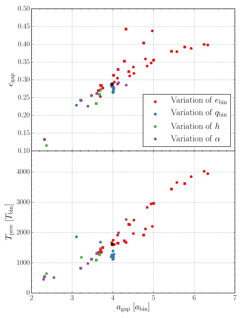
Figure 19: Eccentricity (top) and precession period (bottom) of the inner gap plotted against the semi-major axis of the gap. Different simulation series are colour-coded. Both the measured gap eccentricity and gap semi-major axis are averaged over several thousand binary orbits. Pluto simulations are represented by dots and squares stand for Rh2d simulations. The reference model with Kepler-16 parameters is marked with the star.

To allow for an alternative view of the impact of different binary and disc parameters on the dynamical structure of the disc we display in Fig. 19 the eccentricity (top) and the precession period (bottom) of the gap plotted against the semi-major axis of the gap for all our simulations where different colours stand for different model series. Pluto simulations are represented by dots whereas squares stand for Rh2d simulations. The reference model is marked with a star. Interestingly the majority of the models lie on a main-sequence branch, which has the trend of increasing eccentricity and precession period with increasing gap width. The smaller branch that bifurcates near the reference model represents the low $e_{\mathrm{bin}}$ sequence, which has higher $e_{\mathrm{gap}}$ but smaller $T_{\mathrm{prec}}$. By coincidence, our reference model with the Kepler-16 parameters lies near the bifurcation point.

How the location of the bifurcation point depends of the disc and binary parameter needs to be explored in subsequent numerical studies. A first simulation series with $q_{\mathrm{bin}}=0.6$ suggest that this critical eccentricity does not depend on the mass ratio of the binary. As outlined in the Appendix, for parameters very near to the critical $e_{\mathrm{bin}}$ the models can have the tendency to switch between the two states during a single simulation. The physical cause of the bifurcation needs to be analysed in subsequent simulations.

In addition, there are a more possibilities to further improve our model. First, the use of a non-isothermal equation should be considered to study the effects of viscous heating and radiative cooling. Especially for simulations, which also evolve planets inside the disc, Kley & Haghighipour (2014) showed that radiative effects should been taken into account. Self-gravity effects have been studied by Lines et al. (2015) and Mutter et al. (2017) and are important for galactic discs around a central binary black hole. The backreaction of the disc onto the binary could also be considered in more detail. Angular momentum exchange with the binary occurs through gravitational torques from the disc and direct accretion of angular momentum from the material that enters the central cavity. The first part always leads a decrease in the binary semi-major axis and an increase in eccentricity (Kley & Haghighipour, 2015), while Miranda et al. (2017) pointed out that angular momentum advection might even be dominant leading to a binary separation.

Another interesting question is the evolution of planets inside the circumbinary disc and their influence on the disc structure. Since an in situ formation of the observed planets seems very unlikely, the migration and final parking position of planets is an interesting topic that requires further investigations. In view of our extensive parameter studies there is the indication that in several past studies (Pierens & Nelson, 2013; Kley & Haghighipour, 2014, 2015) an inner radius was considered that was too large and that did not allow for full disc dynamics.

Through fully three-dimensional simulations it will be possible to study the dynamical evolution of inclined discs.

Appendix A Convergence study

The strong gravitational influence of the binary onto the disc, and the complex dynamics of the inner disc presents a big challenge for numerical schemes of grid codes. We therefore study in this appendix the dependence of the disc structure on numerical parameters, such as the numerical scheme or the grid resolution. First, we simulated our reference system, using an open inner boundary and an inner radius of $R_{\mathrm{min}}=$0.25\text{\,}\mathrm{a}\mathrm{u}$$, with the different codes described in Sec. 3.

In Fig. 20 the long-time evolution of the disc eccentricity (top) and of the longitude of periastron (bottom) are shown. All three codes produce comparable results, although we should note that to get this agreement simulations performed with Pluto need a slightly higher resolution. Pluto simulations with a resolution of $448\times 512$ grid cells produce a slightly smaller precession period of the inner disc (red line in Fig. 22, see also Table 3). One possible explanation for this could be the size of the numerical stencil. Fargo and Rh2d have a very compact stencil because they use a staggered grid. In contrast, Pluto has a wider stencil because a collocated grid is used, where all variables are defined at the cell centres. In particular the viscosity routine of Pluto has a very wide stencil to achieve the correct centring of the viscous stress tensor components. This could explain why for Pluto a slightly higher resolution is needed.

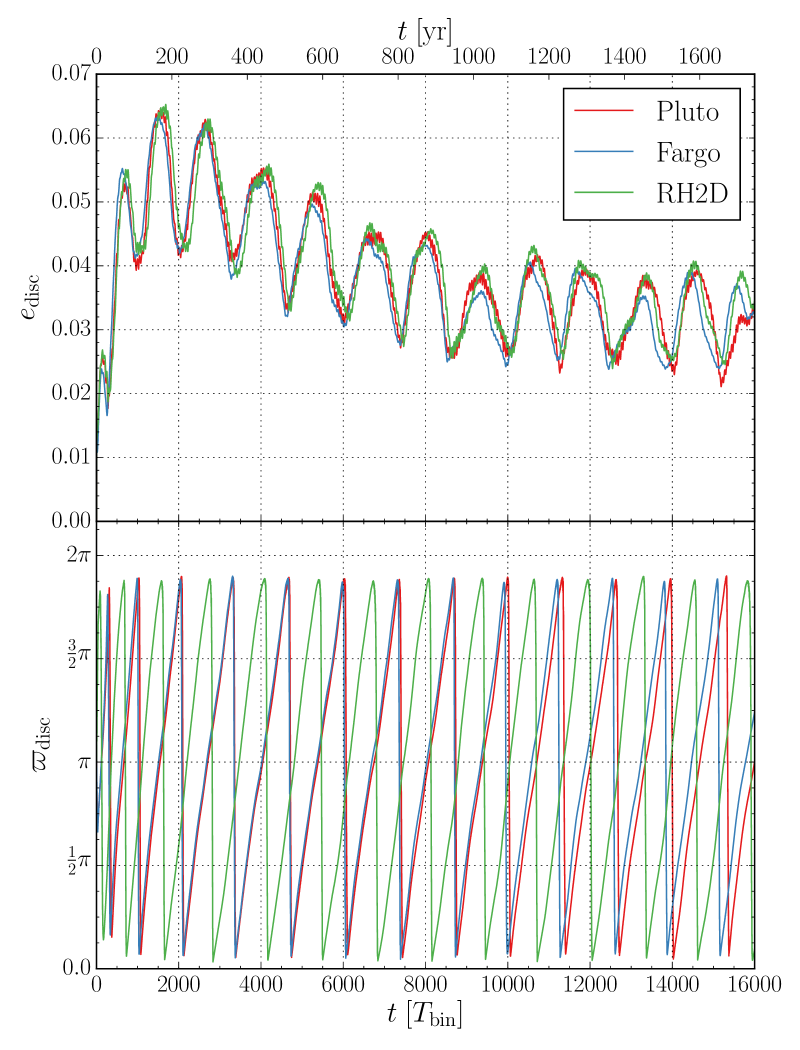
Figure 20: Comparison of disc eccentricity (top) and disc longitude of pericentre (bottom) for the standard model. The disc eccentricity was calculated by summing over the whole disc ($R_{2}=R_{\mathrm{max}}$ in equation (18)), whereas the disc longitude of pericentre was calculated only for the inner disc ($R_{2}=$1.0\text{\,}\mathrm{a}\mathrm{u}$$ in equation (19)). The $\pi$-shift of the green curve in the bottom panel is explained in the text. We used a resolution of $512\times 580$ grid cells for Pluto simulations and for Fargo and Rh2d simulations a resolution of $448\times 512$.

The $\pi$-shift of the longitude of periastron calculated with Rh2d compared to the values calculated with Pluto and Fargo (bottom Panel of Fig. 20) can be explained in the following way. Simulations performed with Pluto and Fargo started the binary at periastron with the pericentre of the secondary at $\varphi=\pi$ (see red ellipses in Fig. 8), whereas Rh2d started the binary at apastron with the pericentre of the secondaries orbit at $\varphi=0$. The data show that when the disc eccentricity is at its maximum the disc is aligned with the orbit of the secondary star. Since the pericentre of the secondary in Rh2d simulations is shifted by $\pi$ we can also see this $\pi$-shift in the disc’s longitude of periastron.

Fig. 21 shows the azimuthally averaged density profiles at $t=$16\,000$\,T_{\mathrm{bin}}$. Even after such a long time span all three codes agree very closely. All codes produce roughly the same density maximum and the same density slopes.

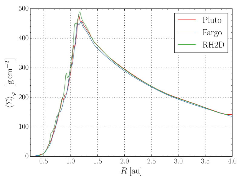
Figure 21: Azimuthally averaged density profiles calculated with different codes at $t=$16\,000$\,T_{\mathrm{bin}}$.

To check the influence of the numerical resolution on the disc structure we run Pluto simulations with different resolutions, summarised in Table 3. The results of this resolution test are shown in Fig. 22.

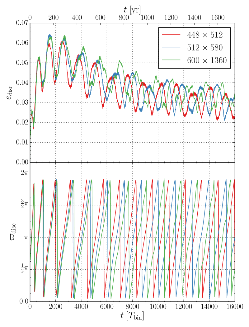
Figure 22: Comparison of different resolutions. Top: Disc eccentricity. Bottom: Disc longitude of pericentre. All simulations were performed with Pluto.

The disc eccentricity converges to the same value, whereas it seems that the disc precession rates increases with higher resolution. A closer look at the data shows that after around $6000$ orbits the precession rate for the higher resolution converged. Table 3 summarises the measured precession rate for different resolutions. Since there is no large variation between $512\times 580$ and $600\times 1360$ grid cells, we used a resolution of $512\times 580$ grid cells for our Pluto simulations.

Table 3: Disc precession rate for different resolutions.

Resolution	$T_{\mathrm{prec}}\,[T_{\mathrm{bin}}]$
$448\times 512$	$1277.49$
$512\times 580$	$1321.48$
$600\times 1360$	$1349.50$

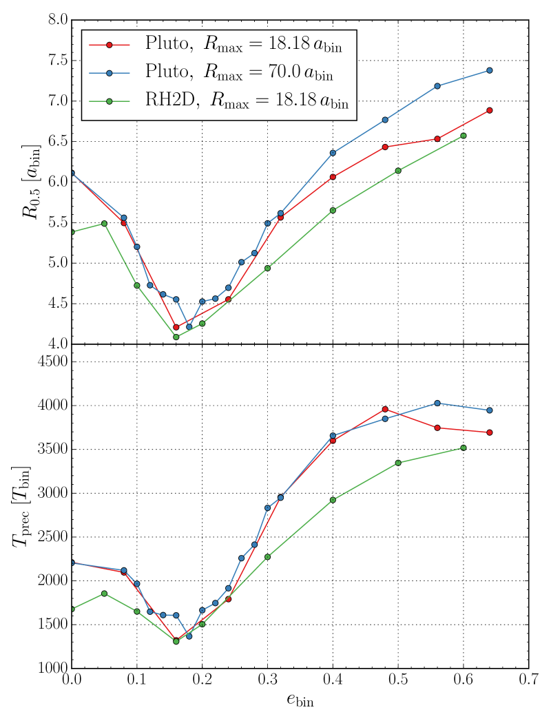
Figure 23: Influence of different outer radii on gap size and precession rate while varying the binary eccentricity. Top: Radius where the azimuthally averaged surface density drops to 50 percent of its maximum value. Bottom: Precession period of the disc gap.

As already discussed in Sect. 4.2 in some cases (for example high binary eccentricities) an outer radius of $R_{\mathrm{max}}=$4.0\text{\,}\mathrm{a}\mathrm{u}$$ can lead to wave reflections which interfere with the inner disc. Therefore we increased the outer boundary to $R_{\mathrm{max}}=$15.4\text{\,}\mathrm{a}\mathrm{u}$=70\,a_{\mathrm{bin}}$ (and to ensure the same resolution between $0.25\text{\,}\mathrm{a}\mathrm{u}$ and $4.0\text{\,}\mathrm{a}\mathrm{u}$ we also increased the number of grid points to $762\times 582$). Figure 23 compares the effect of different outer radii for the case of varying binary eccentricities. For binary eccentricities greater than $0.32$, a larger outer radius makes a difference. Also, around the bifurcation point, at $e_{\mathrm{bin}}=0.18$, a larger outer radius changes the gap size and precession rate of the disc. We also added results from Rh2d simulations with an outer radius of $R_{\mathrm{max}}=18.18\,a_{\mathrm{bin}}$. These Rh2d results follow the same trend as the Pluto simulations, although for most binary eccentricities we could not reproduce the very good agreement of the $e_{\mathrm{bin}}=0.16$ case. Around $e_{\mathrm{bin}}=0.18$, which is the critical binary eccentricity where the two branches bifurcate, simulations tend to switch between two states. This jump happens after roughly $3000$ binary orbits and does not depend on physical parameters. Changes in numerical parameters, like the Courant-Friedrichs-Lewy condition or $R_{\mathrm{max}}$, can trigger the jump. This can be seen in Fig. 23 for $e_{\mathrm{bin}}=0.16$ where simulations with $R_{\mathrm{max}}=18.18\,a_{\mathrm{bin}}$ (red curve) and $R_{\mathrm{max}}=70.0\,a_{\mathrm{bin}}$ (blue curve) produce different values for the gap size and the precession period. An outer radius of $R_{\mathrm{max}}=18.18\,a_{\mathrm{bin}}$ is in the case of $e_{\mathrm{bin}}=0.16$ not too small, since a simulation with $R_{\mathrm{max}}=100\,a_{\mathrm{bin}}$ again produced the same values for the gap size and the precession period. For simulations with $e_{\mathrm{bin}}$ far away from $e_{\mathrm{crit}}$, we did not observe these jumps between states. So far we have only observed these jumps in simulations carried out with Pluto.

Appendix B Comparison with massless test particle

In our circumbinary disc evolution we found that the inner disc becomes eccentric with a constant precession rate. In this section we compare this to test particle trajectories around the binary and investigate how a massless particle with orbital elements similar to the disc gap (Fig. 19) would behave under the influence of the binary potential. In particular, we would like to know at what distance from the binary a test particle has to be positioned such that its precession period agrees approximately with that of the disc. Using secular perturbation theory for the coplanar motion of a massless test particle around an eccentric binary star Moriwaki & Nakagawa (2004) derived the following formula for the particle’s precession period for low binary eccentricities

$$T_{\mathrm{prec}}=\frac{4}{3}\frac{(q_{\mathrm{bin}}+1)^{2}}{q_{\mathrm{bin}}}\left(\frac{a_{\mathrm{p}}}{a_{\mathrm{bin}}}\right)^{7/2}\left(1+\frac{3}{2}e_{\mathrm{bin}}^{2}\right)^{-1}T_{\mathrm{bin}}\,,$$ (26)

where $a_{\mathrm{p}}$ is the semi-major axis of the particle. The same relation was quoted by Miranda et al. (2017) based on results by Liu et al. (2015). A similar relation was given by Leung & Lee (2013) without the $e_{\mathrm{bin}}$ term.

In order to verify the applicability of expression (26) when varying of binary and planet parameters, we performed series of three-body simulations with very low planet mass ($10^{-6}M_{\odot}$), where we varied individually $q_{\mathrm{bin}}$, $e_{\mathrm{bin}}$, and $a_{\mathrm{p}}$. In addition we varied the planet eccentricity $e_{\mathrm{p}}$. For the simulations we used the parameter of the Kepler-16 systems as a reference (see Table 1) and integrated the system for several $10\,000$ binary orbits. Our results of these three-body simulations are shown in Fig. 24. We find that the precession rate scales with $q_{\mathrm{bin}}$, $a_{\mathrm{p}}$, and $e_{\mathrm{bin}}$ exactly as expected from relation (26). The fourth panel of Fig. 24 indicates that the precession period also depends on the particle eccentricity as $T_{\mathrm{prec}}\sim(1-e_{\mathrm{p}}^{2})^{2}$, where we plotted the average eccentricity of the orbit which is equivalent to the particle’s free eccentricity. The agreement holds up to about $e_{\mathrm{p}}^{2}\sim 0.5$ for the used $a_{\mathrm{p}}$. Clearly, for higher values of $e_{\mathrm{p}}$ the particle’s orbit will be unstable as this leads to close encounters with the binary. The value of $e_{\mathrm{p}}$ where this happens depends on the distance from the binary star. For lower $a_{\mathrm{p}}$ the range will be more limited. In summary, we find for the precession period of a particle around a binary star

$$T_{\mathrm{prec}}=\frac{4}{3}\frac{(q_{\mathrm{bin}}+1)^{2}}{q_{\mathrm{bin}}}\left(\frac{a_{\mathrm{p}}}{a_{\mathrm{bin}}}\right)^{7/2}\frac{\left(1-e_{\mathrm{p}}^{2}\right)^{2}}{\left(1+\frac{3}{2}e_{\mathrm{bin}}^{2}\right)}\,T_{\mathrm{bin}}\,.$$ (27)

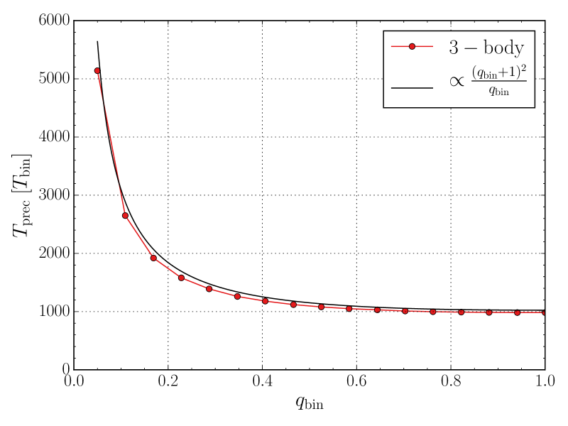
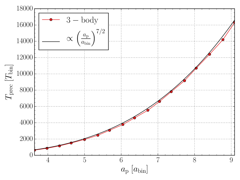
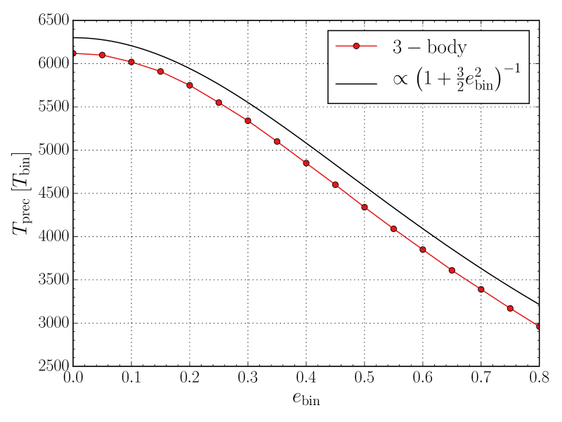
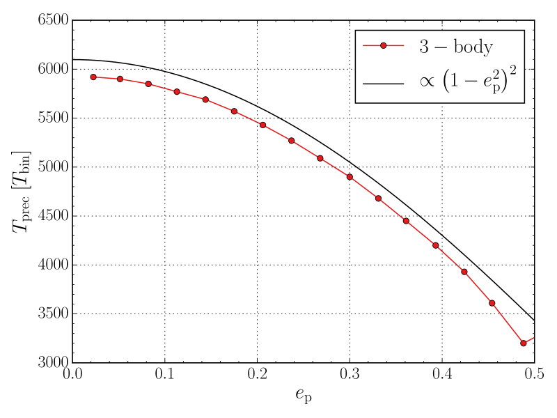
Figure 24: Scaling of the precession period of a particle orbiting a binary stars. As base binary parameter we chose the Kepler-16 parameters and for the planet $a_{\mathrm{p}}=$1.50\text{\,}\mathrm{a}\mathrm{u}$$ and $e_{\mathrm{p}}=0.05$. As an exception we chose for the 1st panel $a_{\mathrm{p}}=$1.0\text{\,}\mathrm{a}\mathrm{u}$$. The black curves refer directly to eq. (27) and the corresponding scaling is indicated.

This relation is plotted in Fig. 24 as the solid black line. In addition to the scaling behaviour we find that the numerical results are about $3-5\%$ lower than the theoretical estimate. The agreement of the numerical results with the theoretical prediction becomes better for larger $a_{\mathrm{p}}$ because eq. (27) is derived from an approximation for large $a_{\mathrm{p}}/a_{\mathrm{bin}}$. The full relation (27) can be inferred directly from eq. (11) in Georgakarakos & Eggl (2015).

Now we compare the particle precession rate to our disc simulations. The best option for this comparison is to check the scaling of the precession rate for models where $q_{\mathrm{bin}}$ has been varied because for binary mass ratio greater than $q_{\mathrm{bin}}=0.3$ the gap size and eccentricity do not change much (purple points in Fig. 19). This is supported by the small variation of the gap radii in Fig. 16. For higher mass ratios the gap size is approximately $a_{\mathrm{gap}}=4.0\,a_{\mathrm{bin}}$ and $e_{\mathrm{gap}}=0.27$. As seen from eq. (27), a test particle with these orbit elements would have a precession period that is far too short. However, if we assume that the test particle has a semi-major axis of $a_{p}=4.9\,a_{\mathrm{bin}}$ (roughly 20 percent more than $a_{\mathrm{gap}}$), the precession period of the gap and the particle match very well for different $q_{\mathrm{bin}}$ (Fig. 25), at least for the higher mass ratios. In general, however, due to the strong sensitivity of the precession period with $a_{\mathrm{p}}$, an exact agreement will be difficult to obtain.

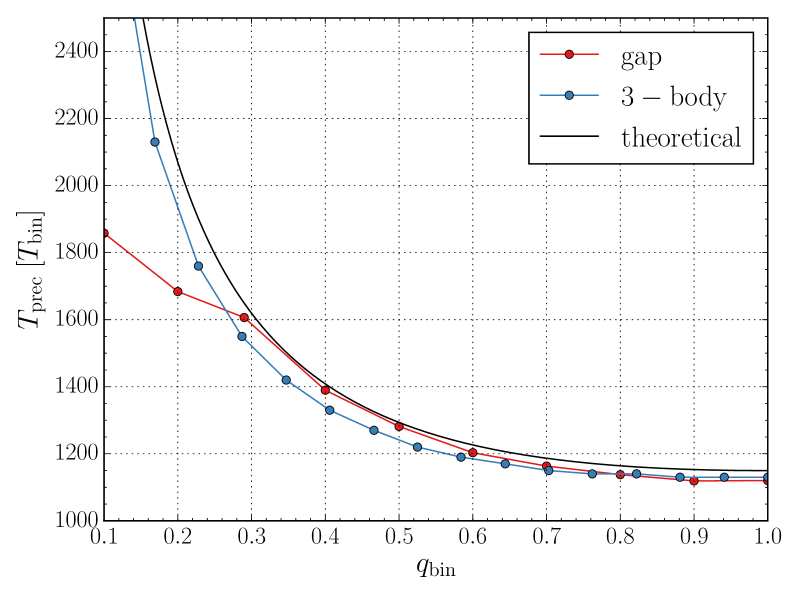
Figure 25: Comparison of the precession period of the inner disc with the precession period of free particle. For the particle we used $a_{\mathrm{p}}=4.9\,a_{\mathrm{bin}},e_{\mathrm{p}}=0.25$. To obtain the shown agreement the particle’s semi-major axis $a_{\mathrm{p}}$ has to be roughly 20 percent longer than $a_{\mathrm{gap}}$. The theoretical line was calculated with equation (27).