Stochastic Quasi-Fejér Block-Coordinate Fixed Point Iterations With Random Sweeping II: Mean-Square and Linear Convergence

Abstract

Reference [11] investigated the almost sure weak convergence of block-coordinate fixed point algorithms and discussed their applications to nonlinear analysis and optimization. This algorithmic framework features random sweeping rules to select arbitrarily the blocks of variables that are activated over the course of the iterations and it allows for stochastic errors in the evaluation of the operators. The present paper establishes results on the mean-square and linear convergence of the iterates. Applications to monotone operator splitting and proximal optimization algorithms are presented.

Keywords. Block-coordinate algorithm, fixed-point algorithm, mean-square convergence, monotone operator splitting, linear convergence, stochastic algorithm

1 Introduction

In [11], we investigated the asymptotic behavior of abstract stochastic quasi-Fejér fixed point iterations in a Hilbert space ${\boldsymbol{\mathsf{H}}}$ and applied these results to establish almost sure convergence properties for randomly activated block-coordinate, stochastically perturbed extensions of algorithms employed in fixed point theory, monotone operator splitting, and optimization. The basic property of the operators used in the underlying model was that of quasinonexpansiveness. Recall that an operator $\boldsymbol{\mathsf{T}}\colon{\boldsymbol{\mathsf{H}}}\to{\boldsymbol{\mathsf{H}}}$ with fixed point set $\text{\rm Fix}\,\boldsymbol{\mathsf{T}}$ is quasinonexpansive if

$$(\forall\boldsymbol{\mathsf{z}}\in\text{\rm Fix}\,\boldsymbol{\mathsf{T}})(\forall\boldsymbol{\mathsf{x}}\in{\boldsymbol{\mathsf{H}}})\quad\|\boldsymbol{\mathsf{T}}\boldsymbol{\mathsf{x}}-\boldsymbol{\mathsf{z}}\|\leqslant\|\boldsymbol{\mathsf{x}}-\boldsymbol{\mathsf{z}}\|,$$ (1.1)

and strictly quasinonexpansive if the above inequality is strict whenever $\boldsymbol{\mathsf{x}}\not\in\text{\rm Fix}\,\boldsymbol{\mathsf{T}}$ [6]. The fixed point problem under investigation in [11] was the following.

Problem 1.1

Let $({\mathsf{H}}_{i})_{1\leqslant i\leqslant m}$ be separable real Hilbert spaces and let ${\boldsymbol{\mathsf{H}}}={\mathsf{H}}_{1}\oplus\cdots\oplus{\mathsf{H}}_{m}$ be their direct Hilbert sum. For every $n\in\mathbb{N}$, let $\boldsymbol{\mathsf{T}}_{\!n}\colon{\boldsymbol{\mathsf{H}}}\to{\boldsymbol{\mathsf{H}}}\colon\boldsymbol{\mathsf{x}}\mapsto({\mathsf{T}}_{\!i,n}\,\boldsymbol{\mathsf{x}})_{1\leqslant i\leqslant m}$ be a quasinonexpansive operator where, for every $i\in\{1,\ldots,m\}$, ${\mathsf{T}}_{\!i,n}\colon{\boldsymbol{\mathsf{H}}}\to{\mathsf{H}}_{i}$ is measurable. Suppose that $\boldsymbol{\mathsf{F}}=\bigcap_{n\in\mathbb{N}}\text{\rm Fix}\,\boldsymbol{\mathsf{T}}_{\!n}\neq{\varnothing}$. The problem is to find a point in $\boldsymbol{\mathsf{F}}$.

In [11], Problem 1.1 was solved via the following block-coordinate algorithm. The main advantages of a block-coordinate strategy is to reduce the computational load and the memory requirements per iteration. In addition, our approach adopts random sweeping rules to select arbitrarily the blocks of variables that are activated at each iteration, and it allows for stochastic errors in the implementation of the operators.

Algorithm 1.2

Let $(\lambda_{n})_{n\in\mathbb{N}}$ be a sequence in $\left]0,1\right]$ and set $\mathsf{D}=\{0,1\}^{m}\smallsetminus\{\boldsymbol{\mathsf{0}}\}$. Let $\boldsymbol{x}_{0}$ and $(\boldsymbol{a}_{n})_{n\in\mathbb{N}}$ be ${\boldsymbol{\mathsf{H}}}$-valued random variables, and let $(\boldsymbol{\varepsilon}_{n})_{n\in\mathbb{N}}$ be identically distributed $\mathsf{D}$-valued random variables. Iterate

$$\begin{array}[]{l}\text{for}\;n=0,1,\ldots\\ \left\lfloor\begin{array}[]{l}\text{for}\;i=1,\ldots,m\\ \left\lfloor\begin{array}[]{l}x_{i,n+1}=x_{i,n}+\varepsilon_{i,n}\lambda_{n}\big{(}{\mathsf{T}}_{\!i,n}\,(x_{1,n},\ldots,x_{m,n})+a_{i,n}-x_{i,n}\big{)}.\end{array}\right.\end{array}\right.\end{array}$$ (1.2)

At iteration $n$ of Algorithm 1.2, $\lambda_{n}\in\left]0,1\right]$ is a relaxation parameter, $a_{i,n}$ an ${\mathsf{H}}_{i}$-valued random variable modeling some stochastic error in the application of the operator $\mathsf{T}_{\!i,n}$, and $\varepsilon_{i,n}$ an $\{0,1\}$-valued random variable that signals the activation of the $i$th block ${\mathsf{T}}_{\!i,n}$ of the operator $\boldsymbol{\mathsf{T}}_{\!n}$. Almost sure weak and strong convergence properties of this scheme were established in [11]. In the present paper, we complement these results by proving mean-square and linear convergence properties for the orbits of (1.2) under the additional assumption that each operator $\boldsymbol{\mathsf{T}}_{\!n}$ in Problem 1.1 satisfies the property

$$(\exists\,\tau_{n}\in\left[0,1\right[)(\forall\boldsymbol{\mathsf{z}}\in\text{\rm Fix}\,\boldsymbol{\mathsf{T}}_{\!n})(\forall\boldsymbol{\mathsf{x}}\in{\boldsymbol{\mathsf{H}}})\quad\|\boldsymbol{\mathsf{T}}_{\!n}\boldsymbol{\mathsf{x}}-\boldsymbol{\mathsf{z}}\|\leqslant\sqrt{\tau_{n}}\|\boldsymbol{\mathsf{x}}-\boldsymbol{\mathsf{z}}\|,$$ (1.3)

which implies that $\boldsymbol{\mathsf{T}}_{\!n}$ is strictly quasinonexpansive and that $\text{\rm Fix}\,\boldsymbol{\mathsf{T}}_{\!n}$ is a singleton. Our results appear to be the first of this kind regarding the block-coordinate algorithm (1.2), even in the case of a single-block, when it reduces to the stochastically perturbed iteration

$$\begin{array}[]{l}\text{for}\;n=0,1,\ldots\\ \left\lfloor\begin{array}[]{l}x_{n+1}=x_{n}+\lambda_{n}\big{(}{\mathsf{T}}_{\!n}x_{n}+a_{n}-x_{n}\big{)},\end{array}\right.\end{array}$$ (1.4)

special cases of which are studied in [2, 12, 24].

The problem we address is more precisely described as follows.

Problem 1.3

Let $({\mathsf{H}}_{i})_{1\leqslant i\leqslant m}$ be separable real Hilbert spaces, set ${\boldsymbol{\mathsf{H}}}={\mathsf{H}}_{1}\oplus\cdots\oplus{\mathsf{H}}_{m}$, and let $\{\tau_{i,n}\}_{1\leqslant i\leqslant m}\subset\left[0,1\right[$. For every $n\in\mathbb{N}$, let $\boldsymbol{\mathsf{T}}_{\!n}\colon{\boldsymbol{\mathsf{H}}}\to{\boldsymbol{\mathsf{H}}}\colon\boldsymbol{\mathsf{x}}\mapsto({\mathsf{T}}_{\!i,n}\,\boldsymbol{\mathsf{x}})_{1\leqslant i\leqslant m}$ be measurable and quasinonexpansive with common fixed point $\overline{\boldsymbol{\mathsf{x}}}=(\overline{\mathsf{x}}_{i})_{1\leqslant i\leqslant m}$, and such that

$$(\forall n\in\mathbb{N})(\forall\boldsymbol{\mathsf{x}}\in{\boldsymbol{\mathsf{H}}})\quad\|\boldsymbol{\mathsf{T}}_{\!n}\boldsymbol{\mathsf{x}}-\overline{\boldsymbol{\mathsf{x}}}\|^{2}\leqslant\sum_{i=1}^{m}\tau_{i,n}\|\mathsf{x}_{i}-\overline{\mathsf{x}}_{i}\|^{2}.$$ (1.5)

The problem is to find $\overline{\boldsymbol{\mathsf{x}}}$.

The proposed mean-square convergence results are the most comprehensive available to date for stochastic block-iterative fixed point methods at the level of generality and flexibility of Algorithm (1.2). Special cases concerning finite-dimensional minimization problems involving a smooth function with restrictions in the implementation of (1.2) are discussed in [18, 20, 21].

The remainder of the paper consists of 3 sections. In Section 2, we provide our notation and preliminary results. Section 3 is dedicated to the mean-square convergence analysis of Algorithm 1.2 and it discusses its linear convergence properties. Applications are presented in Section 4.

2 Notation, background, and preliminary results

Notation. ${\mathsf{H}}$ is a separable real Hilbert space with scalar product ${\left\langle{{\cdot}\mid{\cdot}}\right\rangle}$, associated norm $\|\cdot\|$, Borel $\sigma$-algebra $\mathcal{B}$, and identity operator ${\sf{Id}}\,$. The underlying probability space is $(\Omega,{\mathcal{F}},\mathsf{P})$. A ${\mathsf{H}}$-valued random variable is a measurable map $x\colon(\Omega,{\mathcal{F}})\to({\mathsf{H}},\mathcal{B})$ [14, 15]. The $\sigma$-algebra generated by a family $\Phi$ of random variables is denoted by $\sigma(\Phi)$. Let $\mathscr{F}=({\mathcal{F}}_{n})_{n\in\mathbb{N}}$ be a sequence of sub-sigma algebras of ${\mathcal{F}}$ such that $(\forall n\in\mathbb{N})$ ${\mathcal{F}}_{n}\subset{\mathcal{F}}_{n+1}$. We denote by $\ell_{+}(\mathscr{F})$ the set of sequences of $\left[0,+\infty\right[$-valued random variables $(\xi_{n})_{n\in\mathbb{N}}$ such that, for every $n\in\mathbb{N}$, $\xi_{n}$ is ${\mathcal{F}}_{n}$-measurable. We set

$$(\forall p\in\left]0,+\infty\right[)\quad\ell_{+}^{p}(\mathscr{F})=\left\{{(\xi_{n})_{n\in\mathbb{N}}\in\ell_{+}(\mathscr{F})}~{}\Big{|}~{}{\sum_{n\in\mathbb{N}}\xi_{n}^{p}<{+\infty}\quad\text{\rm$\mathsf{P}$-a.s.}}\right\}.$$ (2.1)

Lemma 2.1

Let $\mathscr{F}=({\mathcal{F}}_{n})_{n\in\mathbb{N}}$ be a sequence of sub-sigma algebras of ${\mathcal{F}}$ such that $(\forall n\in\mathbb{N})$ ${\mathcal{F}}_{n}\subset{\mathcal{F}}_{n+1}$. Let $(\alpha_{n})_{n\in\mathbb{N}}\in\ell_{+}({\mathscr{F}})$, let $(\vartheta_{n})_{n\in\mathbb{N}}\in\ell_{+}({\mathscr{F}})$, let $(\eta_{n})_{n\in\mathbb{N}}\in\ell_{+}({\mathscr{F}})$, and suppose that there exists a sequence $(\chi_{n})_{n\in\mathbb{N}}$ in $\left[0,+\infty\right[$ such that $\varlimsup\chi_{n}<1$ and

$$(\forall n\in\mathbb{N})\quad{\mathsf{E}}(\alpha_{n+1}\!\mid\!{\mathcal{F}}_{n})+\vartheta_{n}\leqslant\chi_{n}\alpha_{n}+\eta_{n}\quad\text{\rm$\mathsf{P}$-a.s.}$$ (2.2)

Then the following hold:

1. Set $(\forall n\in\mathbb{N})$ $\overline{\vartheta}_{n}=\sum_{k=0}^{n}\big{(}\prod_{\ell=k+1}^{n}\chi_{\ell}\big{)}{\mathsf{E}}(\vartheta_{k}\!\mid\!{\mathcal{F}}_{0})$ and $\overline{\eta}_{n}=\sum_{k=0}^{n}\big{(}\prod_{\ell=k+1}^{n}\chi_{\ell}\big{)}{\mathsf{E}}(\eta_{k}\!\mid\!{\mathcal{F}}_{0})$ (with the convention $\prod_{n+1}^{n}\cdot=1$). Then

   $$(\forall n\in\mathbb{N})\quad{\mathsf{E}}(\alpha_{n+1}\!\mid\!{\mathcal{F}}_{0})+\overline{\vartheta}_{n}\leqslant\Bigg{(}\prod_{k=0}^{n}\chi_{k}\Bigg{)}\alpha_{0}+\overline{\eta}_{n}\quad\text{\rm$\mathsf{P}$-a.s.}$$ (2.3)

2. Suppose that $\mathsf{E}\alpha_{0}<{+\infty}$ and $\sum_{n\in\mathbb{N}}\mathsf{E}\eta_{n}<{+\infty}$. Then $\sum_{n\in\mathbb{N}}\mathsf{E}\alpha_{n}<{+\infty}$ and $\sum_{n\in\mathbb{N}}\mathsf{E}\vartheta_{n}<{+\infty}$.

Proof. (i): Let $n\in\mathbb{N}\smallsetminus\{0\}$. We deduce from (2.2) that

$${\mathsf{E}}({\mathsf{E}}(\alpha_{n+1}\!\mid\!{\mathcal{F}}_{n})\!\mid\!{\mathcal{F}}_{n-1})+{\mathsf{E}}(\vartheta_{n}\!\mid\!{\mathcal{F}}_{n-1}) \leqslant{\mathsf{E}}(\chi_{n}\alpha_{n}\!\mid\!{\mathcal{F}}_{n-1})+{\mathsf{E}}(\eta_{n}\!\mid\!{\mathcal{F}}_{n-1})$$

$$=\chi_{n}{\mathsf{E}}(\alpha_{n}\!\mid\!{\mathcal{F}}_{n-1})+{\mathsf{E}}(\eta_{n}\!\mid\!{\mathcal{F}}_{n-1})\quad\text{\rm$\mathsf{P}$-a.s.}$$ (2.4)

However, since ${\mathcal{F}}_{n-1}\subset{\mathcal{F}}_{n}$, we have ${\mathsf{E}}({\mathsf{E}}(\alpha_{n+1}\!\mid\!{\mathcal{F}}_{n})\!\mid\!{\mathcal{F}}_{n-1})={\mathsf{E}}(\alpha_{n+1}\!\mid\!{\mathcal{F}}_{n-1})$. Therefore (2.4) yields

$${\mathsf{E}}(\alpha_{n+1}\!\mid\!{\mathcal{F}}_{n-1})\leqslant\chi_{n}{\mathsf{E}}(\alpha_{n}\!\mid\!{\mathcal{F}}_{n-1})+{\mathsf{E}}(\eta_{n}\!\mid\!{\mathcal{F}}_{n-1})-{\mathsf{E}}(\vartheta_{n}\!\mid\!{\mathcal{F}}_{n-1})\quad\text{\rm$\mathsf{P}$-a.s.}$$ (2.5)

By proceeding by induction and observing that $\alpha_{0}$ is ${\mathcal{F}}_{0}$-measurable, we obtain (2.3).

(ii): We derive from (2.3) that

$$(\forall n\in\mathbb{N})\quad\mathsf{E}\alpha_{n+1}+\mathsf{E}\overline{\vartheta}_{n}\leqslant\Bigg{(}\prod_{k=0}^{n}\chi_{k}\Bigg{)}\mathsf{E}\alpha_{0}+\mathsf{E}\overline{\eta}_{n}=\Bigg{(}\prod_{k=0}^{n}\chi_{k}\Bigg{)}\mathsf{E}\alpha_{0}+\sum_{k=0}^{n}\Bigg{(}\prod_{\ell=k+1}^{n}\chi_{\ell}\Bigg{)}\mathsf{E}\eta_{k}.$$ (2.6)

On the other hand, there exist $q\in\mathbb{N}$ and ${\rho}\in\left]0,1\right[$ such that, for every integer $n>q$, $\chi_{n}<\rho$ and, therefore,

$$\mathsf{E}\alpha_{n+1}+\mathsf{E}\overline{\vartheta}_{n} \leqslant\Bigg{(}\prod_{k=0}^{q}\chi_{k}\Bigg{)}{\rho}^{n-q}\mathsf{E}\alpha_{0}+\sum_{k=0}^{q}\Bigg{(}\prod_{\ell=k+1}^{q}\chi_{\ell}\Bigg{)}{\rho}^{n-q}\mathsf{E}\eta_{k}+\sum_{k=q+1}^{n}{\rho}^{n-k}\mathsf{E}\eta_{k}$$

$$\leqslant\Bigg{(}\prod_{k=0}^{q}\chi_{k}\Bigg{)}{\rho}^{n-q}\mathsf{E}\alpha_{0}+\max\left\{\left(\frac{\prod_{\ell=k+1}^{q}\chi_{\ell}}{{\rho}^{q-k}}\right)_{0\leqslant k\leqslant q},1\right\}\sum_{k=0}^{n}{\rho}^{n-k}\mathsf{E}\eta_{k}.$$ (2.7)

Since $\sum_{n\in\mathbb{N}}{\rho}^{n}<{+\infty}$ and $\sum_{n\in\mathbb{N}}\mathsf{E}\eta_{n}<{+\infty}$, it follows from standard properties of the discrete convolution that $(\sum_{k=0}^{n}{\rho}^{n-k}\mathsf{E}\eta_{k})_{n\in\mathbb{N}}$ is summable. We then deduce from (2) that $\sum_{n\in\mathbb{N}}\mathsf{E}\alpha_{n}<{+\infty}$ and $\sum_{n\in\mathbb{N}}\mathsf{E}\overline{\vartheta}_{n}<{+\infty}$. Thus, the inequalities

$$(\forall n\in\mathbb{N})\quad\mathsf{E}\vartheta_{n}\leqslant\sum_{k=0}^{n}\Bigg{(}\prod_{\ell=k+1}^{n}\chi_{\ell}\Bigg{)}\mathsf{E}\vartheta_{k}=\mathsf{E}\overline{\vartheta}_{n}$$ (2.8)

yield $\sum_{n\in\mathbb{N}}\mathsf{E}\vartheta_{n}<{+\infty}$.      

Lemma 2.2

Let $\phi\colon\left[0,+\infty\right[\to\left[0,+\infty\right[$ be a strictly increasing function such that $\lim_{t\to{+\infty}}\phi(t)={+\infty}$, let $(x_{n})_{n\in\mathbb{N}}$ be a sequence of ${\mathsf{H}}$-valued random variables, and let $({\mathcal{F}}_{n})_{n\in\mathbb{N}}$ be a sequence of sub-sigma-algebras of ${\mathcal{F}}$ such that

$$(\forall n\in\mathbb{N})\quad\sigma(x_{0},\ldots,x_{n})\subset{\mathcal{F}}_{n}\subset{\mathcal{F}}_{n+1}.$$ (2.9)

Suppose that there exist $\mathsf{z}\in{\mathsf{H}}$, $(\vartheta_{n})_{n\in\mathbb{N}}\in\ell_{+}({\mathscr{F}})$, $(\eta_{n})_{n\in\mathbb{N}}\in\ell_{+}({\mathscr{F}})$, and a sequence $(\chi_{n})_{n\in\mathbb{N}}$ in $\left[0,+\infty\right[$ such that $\varlimsup\chi_{n}<1$ and

$$(\forall n\in\mathbb{N})\quad{\mathsf{E}}(\phi(\|x_{n+1}-\mathsf{z}\|)\!\mid\!{\mathcal{F}}_{n})+\vartheta_{n}\leqslant\chi_{n}\phi(\|x_{n}-\mathsf{z}\|)+\eta_{n}\quad\text{\rm$\mathsf{P}$-a.s.}$$ (2.10)

Set $(\forall n\in\mathbb{N})$ $\overline{\vartheta}_{n}=\sum_{k=0}^{n}\big{(}\prod_{\ell=k+1}^{n}\chi_{\ell}\big{)}{\mathsf{E}}(\vartheta_{k}\!\mid\!{\mathcal{F}}_{0})$ and $\overline{\eta}_{n}=\sum_{k=0}^{n}\big{(}\prod_{\ell=k+1}^{n}\chi_{\ell}\big{)}{\mathsf{E}}(\eta_{k}\!\mid\!{\mathcal{F}}_{0})$. Then the following hold:

1. $(\forall n\in\mathbb{N})$ $\displaystyle{\mathsf{E}}(\phi(\|x_{n+1}-\mathsf{z}\|)\!\mid\!{\mathcal{F}}_{0})+\overline{\vartheta}_{n}\leqslant\Bigg{(}\prod_{k=0}^{n}\chi_{k}\Bigg{)}\phi(\|x_{0}-\mathsf{z}\|)+\overline{\eta}_{n}\quad\text{\rm$\mathsf{P}$-a.s.}$

2. Let $p\in\left]0,+\infty\right[$ and set $\phi=|\cdot|^{p}$. Suppose that $x_{0}\in L^{p}(\Omega,{\mathcal{F}},\mathsf{P};{\mathsf{H}})$ and that $\sum_{n\in\mathbb{N}}\mathsf{E}\eta_{n}<{+\infty}$. Then the following hold:

   1. $\mathsf{E}\|x_{n}-\mathsf{z}\|^{p}\to 0$ and $\sum_{n\in\mathbb{N}}\mathsf{E}\vartheta_{n}<{+\infty}$.

   2. Suppose that $(\eta_{n})_{n\in\mathbb{N}}\in\ell_{+}^{1}(\mathscr{F})$. Then $(x_{n})_{n\in\mathbb{N}}$ converges strongly $\mathsf{P}$-a.s. to $\mathsf{z}$.

Proof. We apply Lemma 2.1(i) with $(\forall n\in\mathbb{N})$ $\alpha_{n}=\phi(\|x_{n}-\mathsf{z}\|)$.

(i): See Lemma 2.1(i).

(ii)a): Since $L^{p}(\Omega,{\mathcal{F}},\mathsf{P};{\mathsf{H}})$ is a vector space [25, Théorème 5.8.8 and Proposition 5.8.9] that contains $x_{0}$ and $\mathsf{z}$, it also contains $x_{0}-\mathsf{z}$. Hence $\mathsf{E}\alpha_{0}=\mathsf{E}\|x_{0}-\mathsf{z}\|^{p}<{+\infty}$, and it follows from Lemma 2.1(ii) that $\sum_{n\in\mathbb{N}}\mathsf{E}\|x_{n}-\mathsf{z}\|^{p}<{+\infty}$ and $\sum_{n\in\mathbb{N}}\mathsf{E}\vartheta_{n}<{+\infty}$. Consequently,

$$\mathsf{E}\|x_{n}-\mathsf{z}\|^{p}\to 0.$$ (2.11)

(ii)b): In view of (2.10), since $(\eta_{n})_{n\in\mathbb{N}}\in\ell_{+}^{1}({\mathscr{F}})$, it follows from [12, Proposition 3.1(iii)] that $(\|x_{n}-\mathsf{z}\|)_{n\in\mathbb{N}}$ converges $\mathsf{P}$-a.s.  However, we derive from (2.11) that there exists a strictly increasing sequence $(k_{n})_{n\in\mathbb{N}}$ in $\mathbb{N}$ such that $\|x_{k_{n}}-\mathsf{z}\|\to 0$ $\mathsf{P}$-a.s. [25, Corollaire 5.8.11]. Altogether $\|x_{n}-\mathsf{z}\|\to 0$ $\mathsf{P}$-a.s.      

Theorem 2.3

Let $(\lambda_{n})_{n\in\mathbb{N}}$ be a sequence in $\left]0,1\right]$ such that $\inf_{n\in\mathbb{N}}\lambda_{n}>0$, and let $(t_{n})_{n\in\mathbb{N}}$, $(x_{n})_{n\in\mathbb{N}}$, and $(e_{n})_{n\in\mathbb{N}}$ be sequences of ${\mathsf{H}}$-valued random variables. Further, let $({\mathcal{F}}_{n})_{n\in\mathbb{N}}$ be a sequence of sub-sigma-algebras of ${\mathcal{F}}$ such that

$$(\forall n\in\mathbb{N})\quad\sigma(x_{0},\ldots,x_{n})\subset{\mathcal{F}}_{n}\subset{\mathcal{F}}_{n+1}.$$ (2.12)

Suppose that the following are satisfied:

1. $(\forall n\in\mathbb{N})$ $x_{n+1}=x_{n}+\lambda_{n}(t_{n}+e_{n}-x_{n})$.

2. There exists a sequence $(\xi_{n})_{n\in\mathbb{N}}$ in $\left[0,+\infty\right[$ such that

   $$\sum_{n\in\mathbb{N}}\sqrt{\xi_{n}}<{+\infty}$$ (2.13)

   and $(\forall n\in\mathbb{N})$ ${\mathsf{E}}(\|e_{n}\|^{2}\!\mid\!{\mathcal{F}}_{n})\leqslant\xi_{n}$.

3. There exist $\mathsf{z}\in\mathsf{H}$, $(\theta_{n})_{n\in\mathbb{N}}\in\ell_{+}({\mathscr{F}})$, $(\nu_{n})_{n\in\mathbb{N}}\in\ell_{+}({\mathscr{F}})$, and a sequence $(\mu_{n})_{n\in\mathbb{N}}$ in $\left[0,+\infty\right[$ such that $\varlimsup\mu_{n}<1$ and

   $$(\forall n\in\mathbb{N})\quad{\mathsf{E}}(\|t_{n}-\mathsf{z}\|^{2}\!\mid\!{\mathcal{F}}_{n})+\theta_{n}\leqslant\mu_{n}\|x_{n}-\mathsf{z}\|^{2}+\nu_{n}\quad\text{\rm$\mathsf{P}$-a.s.}$$ (2.14)

Set

$$(\forall n\in\mathbb{N})\quad\begin{cases}\chi_{n}=1-\lambda_{n}+\lambda_{n}\mu_{n}+\sqrt{\xi_{n}}\lambda_{n}\big{(}1-\lambda_{n}+\lambda_{n}\sqrt{\mu_{n}}\big{)}\\ \displaystyle\overline{\vartheta}_{n}=\sum_{k=0}^{n}\Bigg{[}\prod_{\ell=k+1}^{n}\chi_{\ell}\Bigg{]}\lambda_{k}\big{(}{\mathsf{E}}(\theta_{k}\!\mid\!{\mathcal{F}}_{0})+(1-\lambda_{k}){\mathsf{E}}(\|t_{k}-x_{k}\|^{2}\!\mid\!{\mathcal{F}}_{0})\big{)}\\[14.22636pt] \displaystyle\overline{\eta}_{n}=\sum_{k=0}^{n}\Bigg{[}\prod_{\ell=k+1}^{n}\chi_{\ell}\Bigg{]}\lambda_{k}\Big{(}{\mathsf{E}}(\nu_{k}\!\mid\!{\mathcal{F}}_{0})+\big{(}1-\lambda_{k}+\lambda_{k}\big{(}2{\mathsf{E}}(\sqrt{\nu_{k}}\!\mid\!{\mathcal{F}}_{0})+\sqrt{\mu_{k}}\big{)}\big{)}\sqrt{\xi_{k}}+\lambda_{k}\xi_{k}\Big{)}.\end{cases}$$ (2.15)

Then the following hold:

1. $(\forall n\in\mathbb{N})$ $\displaystyle{\mathsf{E}}(\|x_{n+1}-\mathsf{z}\|^{2}\!\mid\!{\mathcal{F}}_{0})+\overline{\vartheta}_{n}\leqslant\Bigg{(}\prod_{k=0}^{n}\chi_{k}\Bigg{)}\|x_{0}-\mathsf{z}\|^{2}+\overline{\eta}_{n}\quad\text{\rm$\mathsf{P}$-a.s.}$

2. Suppose that $x_{0}\in L^{2}(\Omega,{\mathcal{F}},\mathsf{P};{\mathsf{H}})$ and that

   $$\sum_{n\in\mathbb{N}}\sqrt{\mathsf{E}\nu_{n}}<{+\infty}.$$ (2.16)

   Then the following hold:

   1. $\mathsf{E}\|x_{n}-\mathsf{z}\|^{2}\to 0$.

   2. $\sum_{n\in\mathbb{N}}\mathsf{E}\theta_{n}<{+\infty}$.

   3. $\sum_{n\in\mathbb{N}}(1-\lambda_{n})\mathsf{E}\|t_{n}-x_{n}\|^{2}<{+\infty}$.

   4. Suppose that $(\nu_{n})_{n\in\mathbb{N}}\in\ell_{+}^{1/2}({\mathscr{F}})$. Then $(x_{n})_{n\in\mathbb{N}}$ converges strongly $\mathsf{P}$-a.s. to $\mathsf{z}$.

Proof. (i): Set $\lambda=\inf_{n\in\mathbb{N}}\lambda_{n}$. Then

$$(\forall n\in\mathbb{N})\quad\chi_{n}\leqslant 1-(1-\mu_{n}){\lambda}+\sqrt{\xi_{n}}\big{(}1+\sqrt{\mu_{n}}\big{)}.$$ (2.17)

Since $\varlimsup\mu_{n}<1$ and $\lim\xi_{n}=0$, we have $\varlimsup\chi_{n}<1$. In addition, we derive from [a], [6, Corollary 2.15], and (2.14) that

$$(\forall n\in\mathbb{N})\quad \|x_{n+1}-\mathsf{z}\|^{2}$$

$$=\|(1-\lambda_{n})(x_{n}-\mathsf{z})+\lambda_{n}(t_{n}-\mathsf{z})\|^{2}$$

$$\quad+2\lambda_{n}{\left\langle{{(1-\lambda_{n})(x_{n}-\mathsf{z})+\lambda_{n}\big{(}t_{n}-\mathsf{z}\big{)}}\mid{e_{n}}}\right\rangle}+\lambda_{n}^{2}\|e_{n}\|^{2}$$

$$=(1-\lambda_{n})\|x_{n}-\mathsf{z}\|^{2}+\lambda_{n}\|t_{n}-\mathsf{z}\|^{2}-\lambda_{n}(1-\lambda_{n})\|t_{n}-x_{n}\|^{2}$$

$$\quad\;+2\lambda_{n}{\left\langle{{(1-\lambda_{n})(x_{n}-\mathsf{z})+\lambda_{n}\big{(}t_{n}-\mathsf{z}\big{)}}\mid{e_{n}}}\right\rangle}+\lambda_{n}^{2}\|e_{n}\|^{2}\quad\text{\rm$\mathsf{P}$-a.s.}$$ (2.18)

Hence, [c] implies that

$$\hskip-11.38109pt(\forall n\in\mathbb{N})\quad{\mathsf{E}}(\|x_{n+1}-\mathsf{z}\|^{2}\!\mid\!{\mathcal{F}}_{n})$$

$$\leqslant(1-\lambda_{n})\|x_{n}-\mathsf{z}\|^{2}+\lambda_{n}{\mathsf{E}}(\|t_{n}-\mathsf{z}\|^{2}\!\mid\!{\mathcal{F}}_{n})-\lambda_{n}(1-\lambda_{n}){\mathsf{E}}(\|t_{n}-x_{n}\|^{2}\!\mid\!{\mathcal{F}}_{n})$$

$$\quad\;+2\lambda_{n}\big{(}(1-\lambda_{n})\|x_{n}-\mathsf{z}\|+\lambda_{n}\sqrt{{\mathsf{E}}(\|t_{n}-\mathsf{z}\|^{2}\!\mid\!{\mathcal{F}}_{n})}\big{)}\sqrt{{\mathsf{E}}(\|e_{n}\|^{2}\!\mid\!{\mathcal{F}}_{n})}+\lambda_{n}^{2}{\mathsf{E}}(\|e_{n}\|^{2}\!\mid\!{\mathcal{F}}_{n})$$

$$\leqslant(1-\lambda_{n})\|x_{n}-\mathsf{z}\|^{2}+\lambda_{n}\big{(}\mu_{n}\|x_{n}-\mathsf{z}\|^{2}+\nu_{n}-\theta_{n}\big{)}-\lambda_{n}(1-\lambda_{n}){\mathsf{E}}(\|t_{n}-x_{n}\|^{2}\!\mid\!{\mathcal{F}}_{n})$$

$$\quad\;+2\lambda_{n}\big{(}(1-\lambda_{n})\|x_{n}-\mathsf{z}\|+\lambda_{n}\sqrt{\mu_{n}\|x_{n}-\mathsf{z}\|^{2}+\nu_{n}}\big{)}\sqrt{{\mathsf{E}}(\|e_{n}\|^{2}\!\mid\!{\mathcal{F}}_{n})}+\lambda_{n}^{2}{\mathsf{E}}(\|e_{n}\|^{2}\!\mid\!{\mathcal{F}}_{n})\quad\text{\rm$\mathsf{P}$-a.s.}$$ (2.19)

Now set

$$(\forall n\in\mathbb{N})\quad\begin{cases}\vartheta_{n}=\lambda_{n}\theta_{n}+\lambda_{n}(1-\lambda_{n}){\mathsf{E}}(\|t_{n}-x_{n}\|^{2}\!\mid\!{\mathcal{F}}_{n})\\ \kappa_{n}=\lambda_{n}\nu_{n}+2\lambda_{n}^{2}\sqrt{\nu_{n}}\sqrt{{\mathsf{E}}(\|e_{n}\|^{2}\!\mid\!{\mathcal{F}}_{n})}+\lambda_{n}^{2}{\mathsf{E}}(\|e_{n}\|^{2}\!\mid\!{\mathcal{F}}_{n})\\ \eta_{n}=\lambda_{n}\nu_{n}+\lambda_{n}\big{(}1-\lambda_{n}+\lambda_{n}(2\sqrt{\nu_{n}}+\sqrt{\mu_{n}})\big{)}\sqrt{\xi_{n}}+\lambda_{n}^{2}\xi_{n}.\end{cases}$$ (2.20)

It follows from [b] that

$$(\forall n\in\mathbb{N})\quad {\mathsf{E}}(\|x_{n+1}-\mathsf{z}\|^{2}\!\mid\!{\mathcal{F}}_{n})$$

$$\leqslant(1-\lambda_{n}+\lambda_{n}\mu_{n})\|x_{n}-\mathsf{z}\|^{2}+2\lambda_{n}(1-\lambda_{n}+\lambda_{n}\sqrt{\mu_{n}})\|x_{n}-\mathsf{z}\|\sqrt{{\mathsf{E}}(\|e_{n}\|^{2}\!\mid\!{\mathcal{F}}_{n})}$$

$$\quad\;-\vartheta_{n}+\kappa_{n}$$

$$\leqslant(1-\lambda_{n}+\lambda_{n}\mu_{n})\|x_{n}-\mathsf{z}\|^{2}+\lambda_{n}(1-\lambda_{n}+\lambda_{n}\sqrt{\mu_{n}})(\|x_{n}-\mathsf{z}\|^{2}+1)\sqrt{{\mathsf{E}}(\|e_{n}\|^{2}\!\mid\!{\mathcal{F}}_{n})}$$

$$\quad\;-\vartheta_{n}+\kappa_{n}$$

$$\leqslant\chi_{n}\|x_{n}-\mathsf{z}\|^{2}-\vartheta_{n}+\eta_{n}\quad\text{\rm$\mathsf{P}$-a.s.}$$ (2.21)

The result then follows by applying Lemma 2.2(i) with $\phi=|\cdot|^{2}$.

(ii)a): According to (2.20), for every $n\in\mathbb{N}$,

$$\mathsf{E}\eta_{n}= \;\lambda_{n}\mathsf{E}\nu_{n}+\lambda_{n}\big{(}1-\lambda_{n}+\lambda_{n}(2\mathsf{E}\sqrt{\nu_{n}}+\sqrt{\mu_{n}})\big{)}\sqrt{\xi_{n}}+\lambda_{n}^{2}\xi_{n}$$

$$= \;\lambda_{n}\mathsf{E}\nu_{n}+(1-\lambda_{n}+\sqrt{\mu_{n}})\lambda_{n}\sqrt{\xi_{n}}+2\lambda_{n}^{2}\sqrt{\xi_{n}}\,\mathsf{E}\sqrt{\nu_{n}}+\big{(}\lambda_{n}\sqrt{\xi_{n}}\big{)}^{2}$$

$$\leqslant \;\mathsf{E}\nu_{n}+(1+\sqrt{\mu_{n}})\sqrt{\xi_{n}}+2\bigg{(}\sup_{k\in\mathbb{N}}\sqrt{\xi_{k}}\bigg{)}\sqrt{\mathsf{E}\nu_{n}}+\big{(}\sqrt{\xi_{n}}\big{)}^{2},$$ (2.22)

where we have used the fact that $\lambda_{n}\in\left]0,1\right]$ and Jensen’s inequality. We deduce from (2), (2.13), and (2.16) that $\sum_{n\in\mathbb{N}}\mathsf{E}\eta_{n}<{+\infty}$. Hence it follows from (2) and Lemma 2.2(ii)a) that $\mathsf{E}\|x_{n}-\mathsf{z}\|^{2}\to 0$ and that $\sum_{n\in\mathbb{N}}\mathsf{E}\vartheta_{n}<{+\infty}$. In view of (2.20), we obtain (ii)b) and (ii)c).

(ii)d): In view of (2.20), if $(\nu_{n})_{n\in\mathbb{N}}\in\ell_{+}^{1/2}({\mathscr{F}})$, then $(\eta_{n})_{n\in\mathbb{N}}\in\ell_{+}^{1}({\mathscr{F}})$ and the strong convergence claim follows from Lemma 2.2(ii)b).      

Remark 2.4

1. Under the assumptions of Theorem 2.3, if $\nu_{n}\equiv 0$ and $\xi_{n}\equiv 0$, then $\overline{\eta}_{n}\equiv 0$ and it follows from (i) that $({\mathsf{E}}(\|x_{n}-\mathsf{z}\|^{2}\!\mid\!{\mathcal{F}}_{0}))_{n\in\mathbb{N}}$ converges linearly to 0.

2. The weak and strong almost sure convergences of a sequence $(x_{n})_{n\in\mathbb{N}}$ governed by [a] and (2.14) were established in [11, Theorem 2.5] under different assumptions on $(\mu_{n})_{n\in\mathbb{N}}$, $(\nu_{n})_{n\in\mathbb{N}}$, and $(e_{n})_{n\in\mathbb{N}}$.

3 Mean-square and linear convergence of Algorithm 1.2

We complement the almost sure weak and strong convergence results of [11] on the convergence of the orbits of Algorithm 1.2 by establishing mean-square and linear convergence properties.

3.1 Main results

The next theorem constitutes our main result in terms of mean-square convergence. For added flexibility, this convergence will be evaluated in a norm $|||\cdot|||$ on ${\boldsymbol{\mathsf{H}}}$ parameterized by weights $(\omega_{i})_{1\leqslant i\leqslant m}\in\left]0,+\infty\right[^{m}$ and defined by

$$(\forall\boldsymbol{\mathsf{x}}\in{\boldsymbol{\mathsf{H}}})\quad|||\boldsymbol{\mathsf{x}}|||^{2}=\sum_{i=1}^{m}\omega_{i}\|\mathsf{x}_{i}\|^{2}.$$ (3.1)

Theorem 3.1

Consider the setting of Problem 1.3 and Algorithm 1.2, and let $({\mathcal{F}}_{n})_{n\in\mathbb{N}}$ be a sequence of sub-sigma-algebras of ${\mathcal{F}}$ such that

$$(\forall n\in\mathbb{N})\quad\sigma(\boldsymbol{x}_{0},\ldots,\boldsymbol{x}_{n})\subset{\mathcal{F}}_{n}\subset{\mathcal{F}}_{n+1}.$$ (3.2)

Assume that the following are satisfied:

1. $\inf_{n\in\mathbb{N}}\lambda_{n}>0$.

2. There exists a sequence $(\alpha_{n})_{n\in\mathbb{N}}$ in $\left[0,+\infty\right[$ such that $\sum_{n\in\mathbb{N}}\sqrt{\alpha_{n}}<{+\infty}$ and, for every $n\in\mathbb{N}$, ${\mathsf{E}}(\|\boldsymbol{a}_{n}\|^{2}\!\mid\!{\mathcal{F}}_{n})\leqslant\alpha_{n}$.

3. For every $n\in\mathbb{N}$, $\mathcal{E}_{n}=\sigma(\boldsymbol{\varepsilon}_{n})$ and ${\mathcal{F}}_{n}$ are independent.

4. For every $i\in\{1,\ldots,m\}$, $\mathsf{p}_{i}=\mathsf{P}[\varepsilon_{i,0}=1]>0$.

Then the following hold:

1. Let $(\omega_{i})_{1\leqslant i\leqslant m}\in\left]0,+\infty\right[^{m}$ be such that

   $$\begin{cases}(\forall i\in\{1,\ldots,m\})\quad\varlimsup\tau_{i,n}<\omega_{i}\mathsf{p}_{i}\\ \displaystyle\max_{1\leqslant i\leqslant m}\omega_{i}\mathsf{p}_{i}=1,\end{cases}$$ (3.3)

   set

   $$(\forall n\in\mathbb{N})\quad\begin{cases}\xi_{n}=\alpha_{n}\displaystyle{\max_{1\leqslant i\leqslant m}}\;\omega_{i}\\ \displaystyle\mu_{n}=1-\min_{1\leqslant i\leqslant m}\Big{(}\mathsf{p}_{i}-\frac{\tau_{i,n}}{\omega_{i}}\Big{)},\end{cases}$$ (3.4)

   and define

   $$(\forall n\in\mathbb{N})\quad\begin{cases}\chi_{n}=1-\lambda_{n}(1-\mu_{n})+\sqrt{\xi_{n}}\lambda_{n}(1-\lambda_{n}+\lambda_{n}\sqrt{\mu_{n}})\\ \displaystyle\overline{\eta}_{n}=\sum_{k=0}^{n}\Bigg{[}\prod_{\ell=k+1}^{n}\chi_{\ell}\Bigg{]}\lambda_{k}\big{(}1-\lambda_{k}+\lambda_{k}\sqrt{\mu_{k}}+\lambda_{k}\sqrt{\xi_{k}}\big{)}\sqrt{\xi_{k}}.\end{cases}$$ (3.5)

   Then

   $$(\forall n\in\mathbb{N})\;\;\displaystyle\sum_{i=1}^{m}\omega_{i}{\mathsf{E}}(\|x_{i,n+1}-\overline{\mathsf{x}}_{i}\|^{2}\!\mid\!{\mathcal{F}}_{0})\leqslant\Bigg{(}\prod_{k=0}^{n}\chi_{k}\Bigg{)}\Bigg{(}\sum_{i=1}^{m}\omega_{i}\|x_{i,0}-\overline{\mathsf{x}}_{i,0}\|^{2}\Bigg{)}+\overline{\eta}_{n}\quad\text{\rm$\mathsf{P}$-a.s.}$$ (3.6)

2. Suppose that $\boldsymbol{x}_{0}\in L^{2}(\Omega,{\mathcal{F}},\mathsf{P};{\boldsymbol{\mathsf{H}}})$ and $(\forall i\in\{1,\ldots,m\})$ $\varlimsup\tau_{i,n}<1$. Then $\mathsf{E}\|\boldsymbol{x}_{n}-\overline{\boldsymbol{\mathsf{x}}}\|^{2}\to 0$ and $\boldsymbol{x}_{n}\to\overline{\boldsymbol{\mathsf{x}}}$ $\mathsf{P}$-a.s.

Proof. (i): We are going to apply Theorem 2.3 in the Hilbert space $({\boldsymbol{\mathsf{H}}},|||\cdot|||)$ defined by (3.1). Set

$$(\forall n\in\mathbb{N})\quad\boldsymbol{t}_{n}=\big{(}x_{i,n}+\varepsilon_{i,n}({\mathsf{T}}_{\!i,n}\,\boldsymbol{x}_{n}-x_{i,n})\big{)}_{1\leqslant i\leqslant m}\quad\text{and}\quad\boldsymbol{e}_{n}=(\varepsilon_{i,n}a_{i,n})_{1\leqslant i\leqslant m}.$$ (3.7)

Then it follows from (1.2) that

$$(\forall n\in\mathbb{N})\quad\boldsymbol{x}_{n+1}=\boldsymbol{x}_{n}+\lambda_{n}\big{(}\boldsymbol{t}_{n}+\boldsymbol{e}_{n}-\boldsymbol{x}_{n}\big{)},$$ (3.8)

while [b] implies that

$$(\forall n\in\mathbb{N})\qquad{\mathsf{E}}(|||\boldsymbol{e}_{n}|||^{2}\!\mid\!{\mathcal{F}}_{n})\leqslant{\mathsf{E}}(|||\boldsymbol{a}_{n}|||^{2}\!\mid\!{\mathcal{F}}_{n})\leqslant\alpha_{n}\max_{1\leqslant i\leqslant m}\omega_{i}=\xi_{n}.$$ (3.9)

We note that it also follows from [b] that $\sum_{n\in\mathbb{N}}\sqrt{\xi_{n}}<{+\infty}$. Now define

$$(\forall n\in\mathbb{N})(\forall i\in\{1,\ldots,m\})\quad\mathsf{q}_{i,n}\colon{\boldsymbol{\mathsf{H}}}\times\mathsf{D}\to\mathbb{R}\colon(\boldsymbol{\mathsf{x}},\boldsymbol{\epsilon})\mapsto\|\mathsf{x}_{i}-\overline{\mathsf{x}}_{i}+\epsilon_{i}({\mathsf{T}}_{\!i,n}\,\boldsymbol{\mathsf{x}}-\mathsf{x}_{i})\|^{2}.$$ (3.10)

Then, for every $n\in\mathbb{N}$ and every $i\in\{1,\ldots,m\}$, the measurability of ${\mathsf{T}}_{\!i,n}$ implies that of the functions $(\mathsf{q}_{i,n}(\cdot,\boldsymbol{\epsilon}))_{\boldsymbol{\epsilon}\in\mathsf{D}}$. However, for every $n\in\mathbb{N}$, [c] asserts that the events $([\boldsymbol{\varepsilon}_{n}=\boldsymbol{\epsilon}])_{\boldsymbol{\epsilon}\in\mathsf{D}}$ constitute an almost sure partition of $\Omega$ and are independent from ${\mathcal{F}}_{n}$, while the random variables $(\mathsf{q}_{i,n}(\boldsymbol{x}_{n},\boldsymbol{\epsilon}))_{\begin{subarray}{c}1\leqslant i\leqslant m\\ \boldsymbol{\epsilon}\in\mathsf{D}\end{subarray}}$ are ${\mathcal{F}}_{n}$-measurable. Therefore, we derive from [16, Section 28.2] that

$$\hskip-17.07164pt(\forall n\in\mathbb{N})(\forall i\in\{1,\ldots,m\})\quad{\mathsf{E}}(\|x_{i,n}+\varepsilon_{i,n}({\mathsf{T}}_{\!i,n}\,\boldsymbol{x}_{n}-x_{i,n})-\overline{\mathsf{x}}_{i}\|^{2}\!\mid\!{\mathcal{F}}_{n})$$

$$\hskip 150.79959pt={\mathsf{E}}\bigg{(}\mathsf{q}_{i,n}(\boldsymbol{x}_{n},\boldsymbol{\varepsilon}_{n})\sum_{\boldsymbol{\epsilon}\in\mathsf{D}}1_{[\boldsymbol{\varepsilon}_{n}=\boldsymbol{\epsilon}]}\!\>\Big{|}\>{\mathcal{F}}_{n}\bigg{)}$$

$$\hskip 150.79959pt=\sum_{\boldsymbol{\epsilon}\in\mathsf{D}}{\mathsf{E}}(\mathsf{q}_{i,n}(\boldsymbol{x}_{n},\boldsymbol{\epsilon})1_{[\boldsymbol{\varepsilon}_{n}=\boldsymbol{\epsilon}]}\!\mid\!{\mathcal{F}}_{n})$$

$$\hskip 150.79959pt=\sum_{\boldsymbol{\epsilon}\in\mathsf{D}}{\mathsf{E}}(1_{[\boldsymbol{\varepsilon}_{n}=\boldsymbol{\epsilon}]}\!\mid\!{\mathcal{F}}_{n})\mathsf{q}_{i,n}(\boldsymbol{x}_{n},\boldsymbol{\epsilon})$$

$$\hskip 150.79959pt=\sum_{\boldsymbol{\epsilon}\in\mathsf{D}}\mathsf{P}[\boldsymbol{\varepsilon}_{n}=\boldsymbol{\epsilon}]\mathsf{q}_{i,n}(\boldsymbol{x}_{n},\boldsymbol{\epsilon})\quad\text{\rm$\mathsf{P}$-a.s.}$$ (3.11)

Combining this identity with (3.1), (3.7), [d], (3.3), and (1.5) yields

$$(\forall n\in\mathbb{N})\quad {\mathsf{E}}(|||\boldsymbol{t}_{n}-\overline{\boldsymbol{\mathsf{x}}}|||^{2}\!\mid\!{\mathcal{F}}_{n})$$

$$=\sum_{i=1}^{m}\omega_{i}\mathsf{E}\Big{(}\big{\|}x_{i,n}+\varepsilon_{i,n}({\mathsf{T}}_{\!i,n}\,\boldsymbol{x}_{n}-x_{i,n})-\overline{\mathsf{x}}_{i}\big{\|}^{2}~{}\Big{|}~{}{\mathcal{F}}_{n}\Big{)}$$

$$=\sum_{i=1}^{m}\omega_{i}\sum_{\boldsymbol{\epsilon}\in\mathsf{D}}\mathsf{P}[\boldsymbol{\varepsilon}_{n}=\boldsymbol{\epsilon}]\mathsf{q}_{i,n}(\boldsymbol{x}_{n},\boldsymbol{\epsilon})$$

$$=\sum_{i=1}^{m}\omega_{i}\left(\sum_{\boldsymbol{\epsilon}\in\mathsf{D},\epsilon_{i}=1}\mathsf{P}[\boldsymbol{\varepsilon}_{n}=\boldsymbol{\epsilon}]\,\|\mathsf{T}_{\!i,n}\,\boldsymbol{x}_{n}-\overline{\mathsf{x}}_{i}\|^{2}+\sum_{\begin{subarray}{c}\boldsymbol{\epsilon}\in\mathsf{D},\,\epsilon_{i}=0\end{subarray}}\mathsf{P}[\boldsymbol{\varepsilon}_{n}=\boldsymbol{\epsilon}]\,\|x_{i,n}-\overline{\mathsf{x}}_{i}\|^{2}\right)$$

$$=\sum_{i=1}^{m}\omega_{i}\mathsf{p}_{i}\|\mathsf{T}_{\!i,n}\,\boldsymbol{x}_{n}-\overline{\mathsf{x}}_{i}\|^{2}+\sum_{i=1}^{m}\omega_{i}(1-\mathsf{p}_{i})\|x_{i,n}-\overline{\mathsf{x}}_{i}\|^{2}$$

$$\leqslant\bigg{(}\max_{1\leqslant i\leqslant m}\omega_{i}\mathsf{p}_{i}\bigg{)}\sum_{i=1}^{m}\|\mathsf{T}_{\!i,n}\,\boldsymbol{x}_{n}-\overline{\mathsf{x}}_{i}\|^{2}+\sum_{i=1}^{m}\omega_{i}(1-\mathsf{p}_{i})\|x_{i,n}-\overline{\mathsf{x}}_{i}\|^{2}$$

$$=|||\boldsymbol{x}_{n}-\overline{\boldsymbol{\mathsf{x}}}|||^{2}+\|\boldsymbol{\mathsf{T}}_{\!n}\boldsymbol{x}_{n}-\overline{\boldsymbol{\mathsf{x}}}\|^{2}-\sum_{i=1}^{m}\omega_{i}\mathsf{p}_{i}\|x_{i,n}-\overline{\mathsf{x}}_{i}\|^{2}$$

$$\leqslant|||\boldsymbol{x}_{n}-\overline{\boldsymbol{\mathsf{x}}}|||^{2}+\sum_{i=1}^{m}(\tau_{i,n}-\omega_{i}\mathsf{p}_{i})\|x_{i,n}-\overline{\mathsf{x}}_{i}\|^{2}$$

$$=\sum_{i=1}^{m}\omega_{i}\Big{(}1+\frac{\tau_{i,n}}{\omega_{i}}-\mathsf{p}_{i}\Big{)}\|x_{i,n}-\overline{\mathsf{x}}_{i}\|^{2}$$

$$\leqslant\left(1-\min_{1\leqslant i\leqslant m}\Big{(}\mathsf{p}_{i}-\frac{\tau_{i,n}}{\omega_{i}}\Big{)}\right)\,|||\boldsymbol{x}_{n}-\overline{\boldsymbol{\mathsf{x}}}|||^{2}\quad\text{\rm$\mathsf{P}$-a.s.}$$ (3.12)

Altogether, properties [a]–[c] of Theorem 2.3 are satisfied with

$$(\forall n\in\mathbb{N})\quad\theta_{n}=\nu_{n}=0.$$ (3.13)

On the other hand, it follows from (3.3) and (3.4) that $\varlimsup\mu_{n}<1$. Hence, we derive from Theorem 2.3(i) that

$$(\forall n\in\mathbb{N})\quad{\mathsf{E}}(|||\boldsymbol{x}_{n+1}-\overline{\boldsymbol{\mathsf{x}}}|||^{2}\!\mid\!{\mathcal{F}}_{0})\leqslant\Bigg{(}\prod_{k=0}^{n}\chi_{k}\Bigg{)}|||\boldsymbol{x}_{0}-\overline{\boldsymbol{\mathsf{x}}}|||^{2}+\overline{\eta}_{n}\quad\text{\rm$\mathsf{P}$-a.s.}$$ (3.14)

(ii): Consider (i) when $(\forall i\in\{1,\ldots,m\})$ $\omega_{i}=1/\mathsf{p}_{i}$. The convergence then follows from the inequalities

$$(\forall\boldsymbol{\mathsf{x}}\in{\boldsymbol{\mathsf{H}}})\quad\min_{1\leqslant i\leqslant m}\mathsf{p}_{i}\,|||\boldsymbol{\mathsf{x}}|||\leqslant\|\boldsymbol{\mathsf{x}}\|\leqslant\max_{1\leqslant i\leqslant m}\mathsf{p}_{i}\,|||\boldsymbol{\mathsf{x}}|||$$ (3.15)

and Theorem 2.3(ii).      

3.2 Linear convergence

As an offspring of the results in Section 3.1, we obtain the following perturbed linear convergence result.

Corollary 3.2

Consider the setting of Problem 1.3 and Algorithm 1.2, suppose that [a]-[d] in Theorem 3.1 are satisfied, and define $(\chi_{n})_{n\in\mathbb{N}}$ and $(\overline{\eta}_{n})_{n\in\mathbb{N}}$ as in (3.5), where

$$\max_{1\leqslant i\leqslant m}\varlimsup\tau_{i,n}<1\quad\text{and}\quad(\forall n\in\mathbb{N})\quad\begin{cases}\xi_{n}=\dfrac{\alpha_{n}}{\displaystyle\min_{1\leqslant i\leqslant m}\mathsf{p}_{i}}\\ \displaystyle\mu_{n}=1-\min_{1\leqslant i\leqslant m}\mathsf{p}_{i}\big{(}1-\tau_{i,n}\big{)}.\end{cases}$$ (3.16)

Then

$$(\forall n\in\mathbb{N})\quad\displaystyle{\mathsf{E}}(\|\boldsymbol{x}_{n+1}-\overline{\boldsymbol{\mathsf{x}}}\|^{2}\!\mid\!{\mathcal{F}}_{0})\leqslant\frac{\displaystyle\max_{1\leqslant i\leqslant m}\mathsf{p}_{i}}{\displaystyle\min_{1\leqslant i\leqslant m}\mathsf{p}_{i}}\Bigg{(}\prod_{k=0}^{n}\chi_{k}\Bigg{)}\|\boldsymbol{x}_{0}-\overline{\boldsymbol{\mathsf{x}}}\|^{2}+\overline{\eta}_{n}\quad\text{\rm$\mathsf{P}$-a.s.}$$ (3.17)

Proof. In view of (3.15), the claim follows from Theorem 3.1(i) applied with $(\forall i\in\{1,\ldots,m\})$ $\omega_{i}=1/\mathsf{p}_{i}$.      

Let us now make some observations to assess the consequences of Corollary 3.2 in terms of bounds on convergence rates, and the potential impact of the activation probabilities of the blocks $(\mathsf{p}_{i})_{1\leqslant i\leqslant m}$ on them. Let us consider the case when $\alpha_{n}\equiv 0$, i.e., when there are no errors. Set

$$(\forall n\in\mathbb{N})\quad\chi_{n}=1-\lambda_{n}\min_{1\leqslant i\leqslant m}\mathsf{p}_{i}(1-\tau_{i,n}).$$ (3.18)

Then we derive from (3.5) and (3.16) that

$$(\forall n\in\mathbb{N})\quad{\mathsf{E}}(\|\boldsymbol{x}_{n+1}-\overline{\boldsymbol{\mathsf{x}}}\|^{2}\!\mid\!{\mathcal{F}}_{0})\leqslant\frac{\displaystyle\max_{1\leqslant i\leqslant m}\mathsf{p}_{i}}{\displaystyle\min_{1\leqslant i\leqslant m}\mathsf{p}_{i}}\Bigg{(}\prod_{k=0}^{n}\chi_{k}\Bigg{)}\|\boldsymbol{x}_{0}-\overline{\boldsymbol{\mathsf{x}}}\|^{2}\quad\text{\rm$\mathsf{P}$-a.s.}$$ (3.19)

Since (3.16) yields $\sup_{n\in\mathbb{N}}\chi_{n}<1$, a linear convergence rate is thus obtained.

For simplicity, let us further assume that the blocks are processed uniformly in the sense that $(\forall i\in\{1,\ldots,m\})$ $\mathsf{p}_{i}=\mathsf{p}$. Set

$$\chi=1-\inf_{n\in\mathbb{N}}\bigg{(}\lambda_{n}\Big{(}1-\max_{1\leqslant i\leqslant m}\tau_{i,n}\Big{)}\bigg{)}\in\left[0,1\right[.$$ (3.20)

Then

$$(\forall n\in\mathbb{N})\quad\chi_{n}=1-\lambda_{n}\mathsf{p}\Big{(}1-\max_{1\leqslant i\leqslant m}\tau_{i,n}\Big{)}\leqslant 1-(1-\chi)\mathsf{p}.$$ (3.21)

When $\mathsf{p}=1$, the upper bound in (3.21) on the convergence rate is minimal and equal to $\chi$. This is consistent with the intuition that frequently activating the coordinates should favor the convergence speed as a function of the iteration number. On the other hand, activating the blocks less frequently induces a reduction of the computational load per iteration. In large scale problems, this reduction may actually be imposed by limited computing or memory resources. In Algorithm 1.2, the cost of computing ${\mathsf{T}}_{\!i,n}(x_{1,n},\ldots,x_{m,n})$ is on the average $\mathsf{p}$ times smaller than in the standard non block-coordinate approach. Hence, if we assume that this cost is independent of $i$ and the iteration number $n$, $N$ iterations of the block-coordinate algorithm have the same computational cost as $\mathsf{p}N$ iterations of a non block-coordinate approach. In view of (3.21), let us introduce the quantity

$$\varrho(\mathsf{p})=-\frac{\ln\big{(}1-(1-{\chi})\mathsf{p}\big{)}}{\mathsf{p}}$$ (3.22)

to evaluate the convergence rate normalized by the probability $\mathsf{p}$ accounting for computational cost. Under the above assumptions, (3.21) yields

$$(\forall n\in\mathbb{N})\quad\prod_{k=0}^{n}\chi_{k}\leqslant\exp\big{(}-\varrho(\mathsf{p})\mathsf{p}(n+1)\big{)}.$$ (3.23)

Elementary calculations show that, if ${\chi}\neq 0$,

$$-\frac{1-{\chi}}{\ln{\chi}}\leqslant\frac{\varrho(\mathsf{p})}{\varrho(1)}\leqslant 1.$$ (3.24)

For example, if ${\chi}>0.2$, then $\varrho(\mathsf{p})/\varrho(1)\in[0.49,1]$. This shows that, for values of ${\chi}$ not too small, the decrease in the normalized convergence rate remains limited with respect to a deterministic approach in which all the blocks are activated. This fact is illustrated by Figure 1, where the graph of $\varrho$ is plotted for several values of $\chi$.

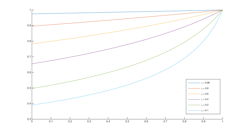
Figure 1: Variations of $\varrho(\mathsf{p})/\varrho(\mathsf{1})$ as a function of $\mathsf{p}$ for various values of $\chi$.

Remark 3.3

Let us consider the special case in which, for every $i\in\{1,\ldots,m\}$, $\tau_{i,n}\equiv\tau_{i}$. Then (3.18) becomes

$$(\forall n\in\mathbb{N})\quad\chi_{n}=1-\lambda_{n}\min_{1\leqslant i\leqslant m}\mathsf{p}_{i}(1-\tau_{i}).$$ (3.25)

Now, let us further assume that, at each iteration $n$, only one of the operators $(\mathsf{T}_{i,n})_{1\leqslant i\leqslant m}$ is activated randomly. In this case, $\sum_{i=1}^{m}\mathsf{p}_{i}=1$ and choosing

$$(\forall i\in\{1,\ldots,m\})\quad\mathsf{p}_{i}=\frac{(1-\tau_{i})^{-1}}{\sum_{j=1}^{m}(1-\tau_{j})^{-1}}.$$ (3.26)

leads to a minimum value of $\chi_{n}$.

4 Applications

In variational analysis, commonly encountered operators include resolvent of monotone operators, projection operators, proximity operators of convex functions, gradient operators, and various compositions and combinations thereof [6, 23]. Specific instances of such operators used in iterative processes which satisfy property (1.5) can be found in [5, 6, 8, 9, 10, 13, 19, 22, 23, 26]. In this section we highlight a couple of examples in the area of splitting methods for systems of monotone inclusions. The notation is that used in Problem 1.3. In addition, let $\mathsf{A}\colon{\mathsf{H}}\to 2^{{\mathsf{H}}}$ be a set-valued operator. We denote by $\text{\rm zer}\,\mathsf{A}=\big{\{}{\mathsf{x}\in{\mathsf{H}}}~{}\big{|}~{}{0\in\mathsf{A}\mathsf{x}}\big{\}}$ the set of zeros of $\mathsf{A}$ and by $\mathsf{J}_{\mathsf{A}}=({\sf{Id}}\,+\mathsf{A})^{-1}$ the resolvent of $\mathsf{A}$. Recall that, if $\mathsf{A}$ is maximally monotone, then $\mathsf{J}_{\mathsf{A}}$ is defined everywhere on ${\mathsf{H}}$ and nonexpansive [6]. In the particular case when $\mathsf{A}$ is the Moreau subdifferential $\partial\mathsf{f}$ of a proper lower semicontinuous convex function $\mathsf{f}\colon{\mathsf{H}}\to\left]-\infty,+\infty\right]$, $\mathsf{J}_{\mathsf{A}}$ is the proximity operator $\text{\rm prox}_{\mathsf{f}}$ of $\mathsf{f}$ [6, 17].

Example 4.1

For every $i\in\{1,\ldots,m\}$, let $\mathsf{A}_{i}\colon{\mathsf{H}}\to 2^{{\mathsf{H}}}$ be a maximally monotone operator, and consider the coupled inclusion problem

$$\text{find}\;\boldsymbol{\mathsf{x}}=(\mathsf{x}_{i})_{1\leqslant i\leqslant m}\in{\boldsymbol{\mathsf{H}}}\;\text{such that}\;\begin{cases}0\in\mathsf{A}_{1}\mathsf{x}_{1}+\mathsf{x}_{1}-\mathsf{x}_{2}\\ 0\in\mathsf{A}_{2}\mathsf{x}_{2}+\mathsf{x}_{2}-\mathsf{x}_{3}\\ \hskip 11.38109pt\vdots&\\ 0\in\mathsf{A}_{m-1}\mathsf{x}_{m-1}+\mathsf{x}_{m-1}-\mathsf{x}_{m}\\ 0\in\mathsf{A}_{m}\mathsf{x}_{m}+\mathsf{x}_{m}-\mathsf{x}_{1}.\end{cases}$$ (4.1)

For instance, in the case when each $\mathsf{A}_{i}$ is the normal cone operator to a nonempty closed convex set, (4.1) models limit cycles in the method of periodic projections [4]. Another noteworthy instance is when $m=2$, $\mathsf{A}_{1}=\partial\mathsf{f}_{1}$, and $\mathsf{A}_{2}=\partial\mathsf{f}_{2}$, where $\mathsf{f}_{1}$ and $\mathsf{f}_{2}$ are proper lower semicontinuous functions from ${\mathsf{H}}$ to $\left]-\infty,+\infty\right]$. Then (4.1) reduces to the joint minimization problem

$$\underset{\begin{subarray}{c}{(\mathsf{x}_{1},\mathsf{x}_{2})\in{\mathsf{H}}^{2}}\end{subarray}}{\text{\rm minimize}}\;\;\mathsf{f}_{1}(\mathsf{x}_{1})+\mathsf{f}_{2}(\mathsf{x}_{2})+\frac{1}{2}\|\mathsf{x}_{1}-\mathsf{x}_{2}\|^{2},$$ (4.2)

studied in [1]. Now set

$$\boldsymbol{\mathsf{A}}\colon\boldsymbol{\mathsf{x}}\mapsto(\mathsf{A}_{1}\mathsf{x}_{1},\ldots,\mathsf{A}_{m}\mathsf{x}_{m})\quad\text{and}\quad\boldsymbol{\mathsf{B}}\colon\boldsymbol{\mathsf{x}}\mapsto(\mathsf{x}_{1}-\mathsf{x}_{2},\mathsf{x}_{2}-\mathsf{x}_{3},\ldots,\mathsf{x}_{m}-\mathsf{x}_{1}).$$ (4.3)

Then it follows from [6, Proposition 20.23] that $\boldsymbol{\mathsf{A}}$ is maximally monotone. On the other hand, $\boldsymbol{\mathsf{B}}$ is linear, bounded, and monotone since

$$(\forall\boldsymbol{\mathsf{x}}\in{\boldsymbol{\mathsf{H}}})\quad{\left\langle{{\boldsymbol{\mathsf{B}}\boldsymbol{\mathsf{x}}}\mid{\boldsymbol{\mathsf{x}}}}\right\rangle}=\dfrac{\|\boldsymbol{\mathsf{B}}\boldsymbol{\mathsf{x}}\|^{2}}{2}\geqslant 0.$$ (4.4)

It is therefore maximally monotone [6, Example 20.34]. Altogether, $\boldsymbol{\mathsf{A}}+\boldsymbol{\mathsf{B}}$ is maximally monotone by [6, Corollary 25.5(i)]. In addition, suppose that each $\mathsf{A}_{i}$ is strongly monotone with constant $\delta_{i}\in\left]0,+\infty\right[$. Then $\boldsymbol{\mathsf{A}}$ is strongly monotone with constant $\min_{1\leqslant i\leqslant m}\delta_{i}$, and so is $\boldsymbol{\mathsf{A}}+\boldsymbol{\mathsf{B}}$. We therefore deduce from [6, Corollary 23.37(ii)] that it possesses a unique zero $\overline{\boldsymbol{\mathsf{x}}}$, which is the unique solution to (4.1). Let us also note that, for every $i\in\{1,\ldots,m\}$, the resolvent $\mathsf{J}_{\mathsf{A}_{i}}$ is Lipschitz continuous with constant $\eta_{i}=1/(1+\delta_{i})\in\left]0,1\right[$ [6, Proposition 23.13]. Next, define $\boldsymbol{\mathsf{T}}\colon{\boldsymbol{\mathsf{H}}}\to{\boldsymbol{\mathsf{H}}}\colon\boldsymbol{\mathsf{x}}\mapsto({\mathsf{T}}_{\!i}\,\boldsymbol{\mathsf{x}})_{1\leqslant i\leqslant m}$, where, for every $i\in\{1,\ldots,m\}$, $\mathsf{T}_{\!i}\colon{\boldsymbol{\mathsf{H}}}\to{\mathsf{H}}_{i}\colon\boldsymbol{\mathsf{x}}\mapsto\mathsf{J}_{\mathsf{A}_{i}}\mathsf{x}_{i+1}$, with the convention $\mathsf{x}_{m+1}=\mathsf{x}_{1}$. Then we derive from (4.1) that $\boldsymbol{\mathsf{T}}\overline{\boldsymbol{\mathsf{x}}}=\overline{\boldsymbol{\mathsf{x}}}$. Moreover,

$$(\forall n\in\mathbb{N})(\forall\boldsymbol{\mathsf{x}}\in{\boldsymbol{\mathsf{H}}})\quad\|\boldsymbol{\mathsf{T}}\boldsymbol{\mathsf{x}}-\overline{\boldsymbol{\mathsf{x}}}\|^{2} =\sum_{i=1}^{m}\|\mathsf{J}_{\mathsf{A}_{i}}\mathsf{x}_{i+1}-\overline{\mathsf{x}}_{i}\|^{2}$$

$$=\sum_{i=1}^{m}\|\mathsf{J}_{\mathsf{A}_{i}}\mathsf{x}_{i+1}-\mathsf{J}_{\mathsf{A}_{i}}\overline{\mathsf{x}}_{i+1}\|^{2}$$

$$\leqslant\sum_{i=1}^{m}\eta^{2}_{i}\|\mathsf{x}_{i+1}-\overline{\mathsf{x}}_{i+1}\|^{2},$$ (4.5)

which shows that (1.5) is satisfied upon choosing $\boldsymbol{\mathsf{T}}_{n}\equiv\boldsymbol{\mathsf{T}}$ and, for every $i\in\{1,\ldots,m\}$, $\tau_{i,n}\equiv\eta_{i}^{2}$. In this scenario, Algorithm 1.2 becomes

$$\begin{array}[]{l}\text{for}\;n=0,1,\ldots\\ \left\lfloor\begin{array}[]{l}\text{for}\;i=1,\ldots,m-1\\ \left\lfloor\begin{array}[]{l}x_{i,n+1}=x_{i,n}+\varepsilon_{i,n}\lambda_{n}\big{(}\mathsf{J}_{\mathsf{A}_{i}}x_{i+1,n}+a_{i,n}-x_{i,n}\big{)}\end{array}\right.\\[2.84526pt] x_{m,n+1}=x_{m,n}+\varepsilon_{m,n}\lambda_{n}\big{(}\mathsf{J}_{\mathsf{A}_{m}}x_{1,n}+a_{m,n}-x_{m,n}\big{)},\end{array}\right.\end{array}$$ (4.6)

and Theorem 3.1 describes its asymptotic behavior. In the particular case of (4.2), for $f_{1}$ and $f_{2}$ strongly convex, (4.6) with $\lambda_{n}\equiv 1$ and no error, reduces to

$$\begin{array}[]{l}\text{for}\;n=0,1,\ldots\\ \left\lfloor\begin{array}[]{l}x_{1,n+1}=x_{1,n}+\varepsilon_{1,n}\big{(}\mathsf{prox}_{\mathsf{f}_{1}}x_{2,n}-x_{1,n}\big{)}\\[2.84526pt] x_{2,n+1}=x_{2,n}+\varepsilon_{2,n}\big{(}\mathsf{prox}_{\mathsf{f}_{2}}x_{1,n}-x_{2,n}\big{)}.\end{array}\right.\end{array}$$ (4.7)

In the deterministic setting in which $\varepsilon_{1,n}\equiv 1$ and $\varepsilon_{2,n}\equiv 1$, the resulting sequence $(x_{2,n})_{n\in\mathbb{N}}$ is that produced by the alternating proximity operator method of [1], further studied in [7].

Example 4.2

We consider an $m$-agent model investigated in [3]. For every $i\in\{1,\ldots,m\}$, let $\mathsf{A}_{i}\colon{\mathsf{H}}_{i}\to 2^{{\mathsf{H}}_{i}}$ be a maximally monotone operator modeling some abstract utility of agent $i$ and let $\mathsf{B}_{i}\colon{\boldsymbol{\mathsf{H}}}\to{\mathsf{H}}_{i}$ be a coupling operator. It is assumed that the operator $\boldsymbol{\mathsf{B}}\colon{\boldsymbol{\mathsf{H}}}\to{\boldsymbol{\mathsf{H}}}\colon\boldsymbol{\mathsf{x}}\mapsto({\mathsf{B}}_{i}\,\boldsymbol{\mathsf{x}})_{1\leqslant i\leqslant m}$ is $\beta$-cocoercive [6] for some $\beta\in\left]0,+\infty\right[$, that is,

$$(\forall\boldsymbol{\mathsf{x}}\in{\boldsymbol{\mathsf{H}}})(\forall\boldsymbol{\mathsf{y}}\in{\boldsymbol{\mathsf{H}}})\quad{\left\langle{{\boldsymbol{\mathsf{x}}-\boldsymbol{\mathsf{y}}}\mid{\boldsymbol{\mathsf{B}}\boldsymbol{\mathsf{x}}-\boldsymbol{\mathsf{B}}\boldsymbol{\mathsf{y}}}}\right\rangle}\geqslant\beta\|\boldsymbol{\mathsf{B}}\boldsymbol{\mathsf{x}}-\boldsymbol{\mathsf{B}}\boldsymbol{\mathsf{y}}\|^{2}.$$ (4.8)

The equilibrium problem is to

$$\text{find}\;\boldsymbol{\mathsf{x}}\in{\boldsymbol{\mathsf{H}}}\;\;\text{such that}\;\;(\forall i\in\{1,\ldots,m\})\quad 0\in\mathsf{A}_{i}\mathsf{x}_{i}+\mathsf{B}_{i}\big{(}\mathsf{x}_{1},\ldots,\mathsf{x}_{m}\big{)}.$$ (4.9)

For every $i\in\{1,\ldots,m\}$, let us further assume that $\mathsf{A}_{i}$ is $\delta_{i}$-strongly monotone for some $\delta_{i}\in\left]0,+\infty\right[$ or, equivalently, that $\mathsf{M}_{i}=\mathsf{A}_{i}-\delta_{i}{\sf{Id}}\,$ is monotone. Since $\boldsymbol{\mathsf{B}}$ is maximally monotone [6, Example 20.31], arguing as in Example 4.1, we arrive at the conclusion that $\boldsymbol{\mathsf{A}}+\boldsymbol{\mathsf{B}}$ has exactly one zero $\overline{\boldsymbol{\mathsf{x}}}$, and that $\overline{\boldsymbol{\mathsf{x}}}$ is the unique solution to (4.9). Let

$$\delta=\min_{1\leqslant i\leqslant m}\delta_{i},\quad\text{and}\quad(\forall n\in\mathbb{N})\quad\theta_{n}\in[0,\delta]\quad\text{and}\quad\gamma_{n}\in\left]0,+\infty\right[.$$ (4.10)

Set

$$(\forall n\in\mathbb{N})\quad\begin{cases}\boldsymbol{\mathsf{C}}_{n}\colon{\boldsymbol{\mathsf{H}}}\to 2^{\boldsymbol{\mathsf{H}}}\colon\boldsymbol{\mathsf{x}}\mapsto\underset{i=1}{\overset{m}{\raisebox{-1.42262pt}{\mbox{\huge{$\times$}}}}}\big{(}\mathsf{M}_{i}+(\delta_{i}-\theta_{n}){\sf{Id}}\,\big{)}\mathsf{x}_{i}\\ \boldsymbol{\mathsf{D}}_{n}=\boldsymbol{\mathsf{B}}+\theta_{n}{\boldsymbol{\sf{Id}}\,}\\[2.84526pt] \boldsymbol{\mathsf{T}}_{n}=\boldsymbol{\mathsf{J}}_{\gamma_{n}\boldsymbol{\mathsf{C}}_{n}}\circ({\boldsymbol{\sf{Id}}\,}-\gamma_{n}\boldsymbol{\mathsf{D}}_{n}).\end{cases}$$ (4.11)

Now let $n\in\mathbb{N}$. We first observe that

$$\text{\rm zer}\,\big{(}\gamma_{n}\boldsymbol{\mathsf{C}}_{n}+\gamma_{n}\boldsymbol{\mathsf{D}}_{n}\big{)}=\text{\rm zer}\,\big{(}\boldsymbol{\mathsf{A}}+\boldsymbol{\mathsf{B}}\big{)}=\{\overline{\boldsymbol{\mathsf{x}}}\}=\text{\rm Fix}\,\boldsymbol{\mathsf{T}}_{n},$$ (4.12)

and derive from [6, Proposition 23.17(i)] that

$$\boldsymbol{\mathsf{J}}_{\gamma_{n}\boldsymbol{\mathsf{C}}_{n}}\colon\boldsymbol{\mathsf{x}}\mapsto\left(\mathsf{J}_{\frac{\gamma_{n}\mathsf{M}_{i}}{1+\gamma_{n}(\delta_{i}-\theta_{n})}}\left(\frac{\mathsf{x}_{i}}{1+\gamma_{n}(\delta_{i}-\theta_{n})}\right)\right)_{1\leqslant i\leqslant m}.$$ (4.13)

Hence (4.10) entails that $\boldsymbol{\mathsf{J}}_{\gamma_{n}\boldsymbol{\mathsf{C}}_{n}}$ is Lipschitz continuous with constant $1/(1+\gamma_{n}({\delta}-\theta_{n}))$. On the other hand, since $\boldsymbol{\mathsf{B}}$ is $\beta$-cocoercive, there exists a nonexpansive operator $\boldsymbol{\mathsf{R}}\colon{\boldsymbol{\mathsf{H}}}\to{\boldsymbol{\mathsf{H}}}$ such that $\beta\boldsymbol{\mathsf{B}}=({\boldsymbol{\sf{Id}}\,}+\boldsymbol{\mathsf{R}})/2$ [6, Remark 4.34(iv)]. We have

$${\boldsymbol{\sf{Id}}\,}-\gamma_{n}\boldsymbol{\mathsf{D}}_{n}=\left(1-\gamma_{n}\theta_{n}-\frac{\gamma_{n}}{2\beta}\right){\boldsymbol{\sf{Id}}\,}-\frac{\gamma_{n}}{2\beta}\boldsymbol{\mathsf{R}}.$$ (4.14)

In turn, a Lipschitz constant of ${\boldsymbol{\sf{Id}}\,}-\gamma_{n}\boldsymbol{\mathsf{D}}_{n}$ is $|1-\gamma_{n}(\theta_{n}+1/(2\beta))|+\gamma_{n}/(2\beta)$, and hence one for $\boldsymbol{\mathsf{T}}_{\!n}$ is

$$\zeta_{n}=\frac{\big{|}1-\gamma_{n}\big{(}\theta_{n}+1/(2\beta)\big{)}\big{|}+\gamma_{n}/(2\beta)}{1+\gamma_{n}(\delta-\theta_{n})}.$$ (4.15)

Note that

$$\zeta_{n}=\begin{cases}\dfrac{1-\gamma_{n}\theta_{n}}{1+\gamma_{n}(\delta-\theta_{n})}<1,&\text{if}\;\;\gamma_{n}\leqslant\dfrac{2\beta}{1+2\beta\theta_{n}};\\[17.07164pt] \dfrac{\gamma_{n}(\theta_{n}+1/\beta)-1}{1+\gamma_{n}(\delta-\theta_{n})}<1,&\text{if}\;\;\dfrac{2\beta}{1+2\beta\theta_{n}}<\gamma_{n}<\dfrac{2\beta}{1+\beta(2\theta_{n}-\delta)}.\end{cases}$$ (4.16)

Consequently, imposing

$$\gamma_{n}<\dfrac{2\beta}{1+\beta(2\theta_{n}-\delta)}$$ (4.17)

places us in the framework of Problem 1.3 with $(\forall i\in\{1,\ldots,m\})$ $\tau_{i,n}=\zeta^{2}_{n}$. Algorithm 1.2 for solving (4.9), that is,

$$\begin{array}[]{l}\text{for}\;n=0,1,\ldots\\ \left\lfloor\begin{array}[]{l}\text{for}\;i=1,\ldots,m\\ \left\lfloor\begin{array}[]{l}\displaystyle x_{i,n+1}=x_{i,n}+\varepsilon_{i,n}\lambda_{n}\bigg{(}\mathsf{J}_{\frac{\gamma_{n}\mathsf{M}_{i}}{1+\gamma_{n}(\delta_{i}-\theta_{n})}}\bigg{(}\frac{(1-\gamma_{n}\theta_{n})x_{i,n}-\gamma_{n}\mathsf{B}_{i}\boldsymbol{x}_{n}}{1+\gamma_{n}(\delta_{i}-\theta_{n})}\bigg{)}+a_{i,n}-x_{i,n}\bigg{)},\end{array}\right.\end{array}\right.\\ \end{array}$$ (4.18)

is then an instance of the block-coordinate forward-backward algorithm of [11, Section 5.2]. Its convergence properties in the present setting are given in Theorem 3.1.

Remark 4.3

In view of (4.4), (4.1) constitutes a special case of (4.9) and it can also be solved via (4.18). In Example 4.1, we have exploited the special structure of $\boldsymbol{\mathsf{B}}$ to obtain tighter coefficients $(\tau_{i,n})_{1\leqslant i\leqslant m,n\in\mathbb{N}}$ in (1.5).

Example 4.4

Let $\boldsymbol{\mathsf{g}}\colon{\boldsymbol{\mathsf{H}}}\to\mathbb{R}$ be a convex function which is differentiable with a $\beta^{-1}$-Lipschitzian gradient for some $\beta\in\left]0,+\infty\right[$ and, for every $i\in\{1,\ldots,m\}$, let $\mathsf{f}_{i}\colon{\mathsf{H}}_{i}\to\left]-\infty,+\infty\right]$ be a proper lower semicontinuous $\delta_{i}$-strongly convex function for some $\delta_{i}\in\left]0,+\infty\right[$. We consider the optimization problem

$$\underset{\begin{subarray}{c}{\mathsf{x}_{1}\in{\mathsf{H}}_{1},\ldots,\mathsf{x}_{m}\in{\mathsf{H}}_{m}}\end{subarray}}{\text{\rm minimize}}\;\;\sum_{i=1}^{m}\mathsf{f}_{i}(\mathsf{x}_{i})+\boldsymbol{\mathsf{g}}(\mathsf{x}_{1},\ldots,\mathsf{x}_{m}).$$ (4.19)

Then it results from standard facts [6, Section 28.5] that this problem is the special case of Example 4.2 in which $\boldsymbol{\mathsf{B}}=\nabla\boldsymbol{\mathsf{g}}$ and, for every $i\in\{1,\ldots,m\}$, $\mathsf{A}_{i}=\partial\mathsf{f}_{i}$. Now set $(\forall i\in\{1,\ldots,m\})$ $\mathsf{h}_{i}=\mathsf{f}_{i}-\delta_{i}\|\cdot\|^{2}/2$. Then (4.18) assumes the form

$$\begin{array}[]{l}\text{for}\;n=0,1,\ldots\\ \left\lfloor\begin{array}[]{l}\text{for}\;i=1,\ldots,m\\ \left\lfloor\begin{array}[]{l}\displaystyle x_{i,n+1}=x_{i,n}+\varepsilon_{i,n}\lambda_{n}\left(\text{\rm prox}_{\frac{\gamma_{n}\mathsf{h}_{i}}{1+\gamma_{n}(\delta_{i}-\theta_{n})}}\bigg{(}\frac{(1-\gamma_{n}\theta_{n})x_{i,n}-\gamma_{n}\nabla_{\!i}\,\boldsymbol{\mathsf{g}}(\boldsymbol{x}_{n})}{1+\gamma_{n}(\delta_{i}-\theta_{n})}\bigg{)}+a_{i,n}-x_{i,n}\right),\end{array}\right.\end{array}\right.\\ \end{array}$$ (4.20)

where $\nabla_{\!i}\,\boldsymbol{\mathsf{g}}\colon{\boldsymbol{\mathsf{H}}}\to{\mathsf{H}}_{i}$ is the $i$th component of $\nabla\boldsymbol{\mathsf{g}}$.

Remark 4.5

In the case of a non block-coordinate implementation, i.e., $m=1$, a mean-square convergence result for the forward-backward algorithm can be found in [24] under different assumptions than ours and, in particular, the requirement that the proximal parameters $(\gamma_{n})_{n\in\mathbb{N}}$ must go to $0$.

Remark 4.6

In connection with the linear convergence of (4.20) deriving from Corollary 3.2, let us note that a similar result was obtained in [20] by imposing the restrictions

$$(\forall i\in\{1,\ldots,m\})\quad{\mathsf{H}}_{i}=\mathbb{R}^{N_{i}},\quad\mathsf{p}_{i}=\frac{1}{m},\quad\text{and}\quad(\forall n\in\mathbb{N})\quad\lambda_{n}=1\quad\text{and}\quad a_{i,n}=0.$$ (4.21)

In this specific setting the proximal parameter in [20] was chosen differently for each block: it is not allowed to vary with the iteration $n$ as in (4.20), but it can be chosen differently for each $i$. In the case when $(\forall i\in\{1,\ldots,m\})$ $\mathsf{f}_{i}=0$, more freedom was given to the choice of $(\mathsf{p}_{i})_{1\leqslant i\leqslant m}$ in [20], but by still activating only one block at each iteration. Further narrowing the problem to the minimization of a smooth strongly convex function on $\mathbb{R}^{N}$, a coordinate descent method is proposed in [21] which requires, for every $i\in\{1,\ldots,m\}$, ${\mathsf{H}}_{i}=\mathbb{R}$ and allows for multiple coordinates to be randomly updated at each iteration, as in (4.20).

References

- [1] F. Acker and M. A. Prestel, Convergence d’un schéma de minimisation alternée, Ann. Fac. Sci. Toulouse V. Sér. Math., vol. 2, pp. 1–9, 1980.
- [2] Y. F. Atchadé, G. Fort, and E. Moulines, On perturbed proximal gradient algorithms, J. Mach. Learn. Res., vol. 18, pp. 1–33, 2017.
- [3] H. Attouch, L. M. Briceño-Arias, and P. L. Combettes, A parallel splitting method for coupled monotone inclusions, SIAM J. Control Optim., vol. 48, pp. 3246–3270, 2010.
- [4] J.-B. Baillon, P. L. Combettes, and R. Cominetti, There is no variational characterization of the cycles in the method of periodic projections, J. Funct. Anal., vol. 262, pp. 400–408, 2012.
- [5] H. H. Bauschke, J. Y. Bello Cruz, T. T. A. Nghia, H. M. Phan, and X. Wang, Optimal rates of linear convergence of relaxed alternating projections and generalized Douglas-Rachford methods for two subspaces, Numer. Algorithms, vol. 73, pp. 33–76, 2016.
- [6] H. H. Bauschke and P. L. Combettes, Convex Analysis and Monotone Operator Theory in Hilbert Spaces, 2nd ed. Springer, New York, 2017.
- [7] H. H. Bauschke, P. L. Combettes, and S. Reich, The asymptotic behavior of the composition of two resolvents, Nonlinear Anal., vol. 60, pp. 283–301, 2005.
- [8] H. H. Bauschke, S. M. Moffat, and X. Wang, Firmly nonexpansive mappings and maximally monotone operators: Correspondence and duality, Set-Valued Var. Anal., vol. 20, pp. 131–153, 2012.
- [9] R. I. Boţ and E. R. Csetnek, Convergence rates for forward-backward dynamical systems associated with strongly monotone inclusions, J. Math. Anal. Appl., vol. 457, pp. 1135–1152, 2018.
- [10] R. I. Boţ, E. R. Csetnek, A. Heinrich, and C. Hendrich, On the convergence rate improvement of a primal-dual splitting algorithm for solving monotone inclusion problems, Math. Programming, vol. 150, pp. 251–279, 2015.
- [11] P. L. Combettes and J.-C. Pesquet, Stochastic quasi-Fejér block-coordinate fixed point iterations with random sweeping, SIAM J. Optim., vol. 25, pp. 1221–1248, 2015.
- [12] P. L. Combettes and J.-C. Pesquet, Stochastic approximations and perturbations in forward-backward splitting for monotone operators, Pure Appl. Funct. Anal., vol. 1, pp. 13–37, 2016.
- [13] P. L. Combettes and B. C. Vũ, Variable metric forward-backward splitting with applications to monotone inclusions in duality, Optimization, vol. 63, pp. 1289–1318, 2014.
- [14] R. M. Fortet, Vecteurs, Fonctions et Distributions Aléatoires dans les Espaces de Hilbert. Hermès, Paris, 1995.
- [15] M. Ledoux and M. Talagrand, Probability in Banach Spaces: Isoperimetry and Processes. Springer, New York, 1991.
- [16] M. Loève, Probability Theory II, 4th ed. Springer, New York, 1978.
- [17] J. J. Moreau, Fonctions convexes duales et points proximaux dans un espace hilbertien, C. R. Acad. Sci. Paris Sér. A Math., vol. 255, pp. 2897–2899, 1962.
- [18] Yu. Nesterov, Efficiency of coordinate descent methods on huge-scale optimization problems, SIAM J. Optim., vol. 22, pp. 341–362, 2012.
- [19] J.-C. Pesquet and N. Pustelnik, A parallel inertial proximal optimization method, Pac. J. Optim., vol. 8, pp. 273–305, 2012.
- [20] P. Richtárik and M. Takáč, Iteration complexity of randomized block-coordinate descent methods for minimizing a composite function, Math. Program., vol. A144, pp. 1–38, 2014.
- [21] P. Richtárik and M. Takáč, On optimal probabilities in stochastic coordinate descent methods, Optim. Lett., vol. 10, pp 1233–1243, 2016.
- [22] R. T. Rockafellar, Monotone operators and the proximal point algorithm, SIAM J. Control Optim., vol. 14, pp. 877–898, 1976.
- [23] R. T. Rockafellar and R. J. B. Wets, Variational Analysis, 3rd printing. Springer-Verlag, New York, 2009.
- [24] L. Rosasco, S. Villa, and B. C. Vũ, Stochastic forward-backward splitting method for solving monotone inclusions in Hilbert spaces, J. Optim. Theory Appl., vol. 169, pp. 388–406, 2016.
- [25] L. Schwartz, Analyse III – Calcul Intégral. Hermann, Paris, 1993.
- [26] M. Sibony, Méthodes itératives pour les équations et inéquations aux dérivées partielles non linéaires de type monotone, Calcolo, vol. 7, pp. 65–183, 1970.