One-loop electron self-energy for the bound-electron $\bm{g}$ factor

Abstract

We report calculations of the one-loop self-energy correction to the bound-electron $g$ factor of the $1s$ and $2s$ states of light hydrogen-like ions with the nuclear charge number $Z\leq 20$. The calculation is carried out to all orders in the binding nuclear strength. We find good agreement with previous calculations and improve their accuracy by about two orders of magnitude.

The bound-electron $g$ factor in light hydrogen-like and lithium-like ions has been measured with a high accuracy, which reached to $3\times 10^{-11}$ in the case of C⁵⁺ sturm:14 . Such measurements have yielded one of the best tests of the bound-state QED theory sturm:11 and significantly improved the precision of the electron mass sturm:14 ; mohr:16:codata . Further advance of the experimental accuracy toward the $10^{-12}$ level is anticipated in the near future sturm:17 .

One of the dominant effects in the bound-electron $g$ factor is the one-loop electron self-energy. Its contribution to the total $g$ factor value is so large that the effect needs to be calculated to all orders in the nuclear binding strength parameter $Z\alpha$ even for ions as light as carbon ($Z$ is the nuclear charge number, $\alpha$ is the fine-structure constant). The numerical error in the evaluation of the electron self-energy is currently the second-largest source of uncertainty for the hydrogen-like ions (the largest error stemming from the two-loop electron self-energy pachucki:04:prl ; pachucki:05:gfact ). The error needs to be descreased in order to match the anticipated experimental precision.

The numerical accuracy of the one-loop self-energy is also relevant for the determination of the electron mass sturm:14 ; mohr:16:codata . The self-energy values actually used in the electron-mass determinations were obtained by an extrapolation of the high- and medium-$Z$ numerical results down to $Z=6$ (carbon) and $8$ (oxygen). Clearly, this situation is not fully satisfactory and a direct numerical calculation would be preferable.

All-order (in $Z\alpha$) calculations of the electron self-energy to the bound-electron $g$ factor have a long history. First calculations of this correction were accomplished two decades ago persson:97:g ; blundell:97 ; beier:00:pra . The numerical accuracy of these evaluations was advanced in the later works yerokhin:02:prl ; yerokhin:04 , which was crucial at the time as it brought an improvement of the electron mass determination. This correction was revisited again in Refs. yerokhin:08:prl ; yerokhin:10:sehfs . In the present work, we aim to advance the numerical accuracy of the one-loop electron self-energy and bring it to the level required for future experiments.

We consider the one-loop self-energy correction to the $g$ factor of an electron bound by the Coulomb field of the point-like and spinless nucleus. This correction can be represented yerokhin:02:prl ; yerokhin:04 as a sum of the irreducible (ir) and the vertex$+$reducible (vr) parts,

$$\Delta g_{\rm SE}=\Delta g_{\rm ir}+\Delta g_{\rm vr}\,.$$ (1)

The irreducible part is

$$\Delta g_{\rm ir}=2\,\langle\delta_{g}a|\gamma^{0}\widetilde{\Sigma}(\varepsilon_{a})|a\rangle\,,$$ (2)

where $\widetilde{\Sigma}(\varepsilon)=\Sigma(\varepsilon)-\delta m$ is the (renormalized) one-loop self-energy operator (see, e.g., yerokhin:10:sehfs ) and $|\delta_{g}a\rangle$ is the perturbed wave function

$$|\delta_{g}a\rangle=\sum_{n\neq a}\frac{|n\rangle\langle n|\delta V_{g}|a\rangle}{\varepsilon_{a}-\varepsilon_{n}}\,,$$ (3)

with $\delta V_{g}=2m[{\bm{r}}\times\bm{\alpha}]_{z}$ being the effective $g$-factor operator yerokhin:10:sehfs that assumes that the spin projection of the reference state is $m_{a}=1/2$. The vertex$+$reducible part is

$$\Delta g_{\rm vr}= \ \frac{i}{2\pi}\int_{C}d\omega\,\sum_{n_{1}n_{2}}\biggl{[}\frac{\langle n_{1}|\delta V_{g}|n_{2}\rangle\langle an_{2}|I(\omega)|n_{1}a\rangle}{(\Delta_{an_{1}}-\omega)(\Delta_{an_{2}}-\omega)}$$

$$-\delta_{n_{1}n_{2}}\,\frac{\langle a|\delta V_{g}|a\rangle\langle an_{1}|I(\omega)|n_{1}a\rangle}{(\Delta_{an_{1}}-\omega)^{2}}\biggr{]}\,,$$ (4)

where $I(\omega)$ is the operator of the electron-electron interaction (see, e.g., yerokhin:04 ), $\omega$ is the energy of the virtual photon, $\Delta_{ab}=\varepsilon_{a}-\varepsilon_{b}$, and a proper covariant identification and cancellation of ultraviolet and infrared divergences is assumed. The integration contour $C$ in Eq. (One-loop electron self-energy for the bound-electron $\bm{g}$ factor) is the standard Feynman integration contour; it will be deformed for a numerical evaluation as discussed below.

The vertex$+$reducible contribution is further divided into three parts: the zero-potential, one-potential, and many-potential contributions,

$$\Delta g_{\rm vr}=\Delta g_{\rm vr}^{(0)}+\Delta g_{\rm vr}^{(1)}+\Delta g_{\rm vr}^{(2+)}\,.$$ (5)

This separation is induced by the following identity, which splits the integrand according to the number of interactions with the binding Coulomb field in the electron propagators,

$$\ G\,\delta V_{g}\,G\equiv\biggl{[}G^{(0)}\,\delta V_{g}\,G^{(0)}\biggr{]}+\biggl{[}G^{(0)}\,\delta V_{g}\,G^{(1)}+G^{(1)}\,\delta V_{g}\,G^{(0)}\biggr{]}$$

$$+\Biggl{[}G\,\delta V_{g}\,G-G^{(0)}\,\delta V_{g}\,G^{(0)}-G^{(0)}\,\delta V_{g}\,G^{(1)}-G^{(1)}\,\delta V_{g}\,G^{(0)}\Biggr{]}\,,$$ (6)

where $G\equiv G(\varepsilon)\equiv\sum_{n}|n\rangle\langle n|/(\varepsilon-\varepsilon_{n})$ is the bound-electron propagator, $G^{(0)}\equiv G\bigr{|}_{Z=0}$ is the free-electron propagator, and

$$G^{(1)}(\varepsilon)\equiv Z\,\left[\frac{d}{dZ}\,G(\varepsilon)\right]_{Z=0}$$

is the one-potential electron propagator.

In the present work, we will be concerned mainly with the numerical evaluation of $\Delta g_{\rm vr}^{(2+)}$, since all other contributions were computed to the required accuracy in our previous investigations yerokhin:04 ; yerokhin:10:sehfs .

After performing integrations over the angular variables analytically as described in Ref. yerokhin:04 , we obtain the result that can be schematically represented as

$$\Delta g_{\rm vr}^{(2+)}=\lim_{|\kappa_{\rm max}|\to\infty}\int_{C}d\omega\,\int_{0}^{\infty}dx\,dy\,dz\,\sum_{|\kappa|=1}^{|\kappa_{\rm max}|}f_{|\kappa|}(\omega,x,y,z)\,,$$ (7)

where $x$, $y$, and $z$ are the radial integration variables, $|\kappa|$ is the absolute value of the angular momentum-parity quantum number of one of the electron propagators, and $f_{|\kappa|}$ is the integrand. Summations over other angular quantum numbers are finite and absorbed into the definition of $f_{|\kappa|}$.

The approach of the present work is to split $\Delta g_{\rm vr}^{(2+)}$ into two parts,

$$\Delta g_{\rm vr}^{(2+)}=\Delta g_{\rm vr,a}^{(2+)}+\Delta g_{\rm vr,b}^{(2+)}$$

$$=\int_{C_{\rm LH,a}}\!\!\!d\omega\,\int_{0}^{\infty}dx\,dy\,dz\,\sum_{|\kappa|=1}^{\kappa_{\rm a}}f_{|\kappa|}(\omega,x,y,z)$$

$$+\lim_{\kappa_{\rm max}\to\infty}\int_{C_{\rm LH,b}}\!\!\!d\omega\,\int_{0}^{\infty}dx\,dy\,dz\,\sum_{|\kappa|=\kappa_{\rm a}+1}^{\kappa_{\rm max}}f_{|\kappa|}(\omega,x,y,z)\,,$$ (8)

where $\kappa_{a}$ is an auxiliary parameter and $C_{\rm LH,a}$ and $C_{\rm LH,b}$ are two integration contours used for the evaluation of the two parts of Eq. (One-loop electron self-energy for the bound-electron $\bm{g}$ factor). In the present work we used $\kappa_{a}=120$, which corresponds to the maximal value of $|\kappa|$ used in Ref. yerokhin:10:sehfs , and $C_{\rm LH,a}$ being the same contour as used in that work. So, the numerical evaluation of $\Delta g_{\rm vr,a}^{(2+)}$ was mostly analogous to the one reported in Ref. yerokhin:10:sehfs , but we had to improve the accuracy of numerical integrations by several orders of magnitude. In the updated numerical integrations, the extended Gauss-log quadratures pachucki:14:cpc were employed, alongside with the standard Gauss-Legendre quadratures.

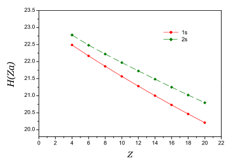
Figure 1: The higher-order remainder function $H(Z\alpha)$, defined by Eq. (One-loop electron self-energy for the bound-electron $\bm{g}$ factor), for the one-loop self-energy correction to the bound-electron $g$ factor of the $1s$ and $2s$ states.

We found it impossible to extend the partial-wave expansion significantly beyond the limit of $\kappa_{a}=120$ within the same numerical scheme as used in Ref. yerokhin:10:sehfs . The reason is that the integration contour $C_{\rm LH,a}$ used there, as well as in our previous works yerokhin:02:prl ; yerokhin:04 , involved computations of the Whittaker functions of the first kind ${{M}_{\alpha,\beta}}(z)$ and their derivatives for large complex values of the argument $z$. The algorithms we use yerokhin:99:pra for computing ${{M}_{\alpha,\beta}}(z)$ become unstable for large $\alpha$ (needed for large $\kappa$’s) and large and complex $z$, even when using the quadruple-precision arithmetics. For this reason, in order to compute $\Delta g_{\rm vr,b}^{(2+)}$, we had to switch to the contour $C_{\rm LH,b}$, which was originally introduced by P. J. Mohr in his calculations of the one-loop self-energy mohr:74:a ; mohr:74:b . The crucial feature of this contour is that it involves the computation of the Whittaker functions ${{M}_{\alpha,\beta}}(z)$ and ${{W}_{\alpha,\beta}}(z)$ of the real arguments $z$ only. For real arguments, the computational algorithms were shown mohr:74:b to be stable even for very large $\kappa$’s (and, hence, $\alpha$’s).

Specifically, the contours $C_{\rm LH,a}$ and $C_{\rm LH,b}$ consist of two parts, the low-energy and the high-energy ones. The low-energy part extends along $(\Delta,0)$ on the lower bank of the cut of the photon propagator of the complex $\omega$ plane and along $(0,\Delta)$ on the upper bank of the cut. The high-energy part consists of the interval $(\Delta,\Delta+i\infty)$ in the upper half-plane and the interval $(\Delta,\Delta-i\infty)$ in the lower half-plane. The difference between $C_{\rm LH,a}$ and $C_{\rm LH,b}$ is only in the choice of the parameter $\Delta$. For $C_{\rm LH,a}$, we use $\Delta=Z\alpha\,\varepsilon_{a}$ (the same choice as in our previous works yerokhin:02:prl ; yerokhin:04 ; yerokhin:10:sehfs ), whereas for $C_{\rm LH,b}$, we use $\Delta=\varepsilon_{a}$ (the Mohr’s choice). Detailed discussion of the integration contour and the analytical properties of the integrand can be found in the original work mohr:74:a .

We found that the price to pay for using the contour $C_{\rm LH,b}$ was the oscillatory behavior of the integrand as a function of the radial variables for $\omega\sim\varepsilon_{a}$. Because of this, we had to employ very dense radial grids for numerical integrations, which made computations rather time-consuming.

The largest error of the numerical evaluation of Eq. (One-loop electron self-energy for the bound-electron $\bm{g}$ factor) comes from the termination of the infinite summation over $|\kappa|$ and the estimation of the tail of the expansion. In the present work, we performed the summation over $|\kappa|$ before all integrations and stored the complete sequence of partial sums, to be used for the extrapolation performed on the last step of the calculation. The convergence of the expansion was monitored; in the cases when the series converged to the prescribed accuracy (i.e., the relative contribution of several consecutive expansion terms was smaller than, typically, $10^{-11}$ for $\Delta g_{\rm vr,a}^{(2+)}$ and $10^{-6}$ for $\Delta g_{\rm vr,b}^{(2+)}$), the summation was terminated. This approach reduced the computation time considerably as compared to our previous scheme yerokhin:04 , where the summation over $|\kappa|$ was performed after all integrations. If the convergence of the partial-wave expansion had not been reached, the summation was extended up to the upper cutoff $\kappa_{\rm max}=450$.

The remaining tail of the series was estimated by analyzing the $|\kappa|$-dependence of the partial-wave expansion terms after all integrations. We fitted the last $m$ expansion terms (typically, $m=20$) to the polynomial in $1/|\kappa|$ with 1-3 fitting parameters,

$$\delta S_{|\kappa|}=c_{0}/|\kappa|^{3}+c_{1}/|\kappa|^{4}+\ldots\,.$$

The uncertainty of the extrapolation was estimated by varying the cutoff parameter $\kappa_{\rm max}$ by 20% and multiplying the resulting difference by a conservative factor of $1.5$. This procedure usually led to the expansion tail estimated with an accuracy of about 10%.

We observed an interesting feature, namely, that the tail of the expansion, with a high accuracy, is the same for the $1s$ and for the $2s$ states. E.g., for $Z=4$, we find the expansion tail of $\delta g(1s)=-1.88\,(19)\times 10^{-12}$ and $\delta g(2s)=-1.88\,(19)\times 10^{-12}$; for $Z=16$, we obtain $\delta g(1s)=-3.00\,(27)\times 10^{-11}$ and $\delta g(2s)=-3.01\,(27)\times 10^{-11}$. We do not know the reason for this but such an agreement shows a high degree of consistency of our numerical calculations for the $1s$ and $2s$ states.

Our numerical results for the self-energy correction to the bound-electron $g$ factor of the $1s$ and $2s$ states of hydrogen-like ions are presented in Table Acknowledgement. The values for the irreducible part $\Delta g_{\rm ir}$ are taken from our previous investigations (from Ref. yerokhin:10:sehfs for $Z\leq 12$ and from Ref. yerokhin:04 otherwise). Using results of Ref. yerokhin:04 , we introduced small corrections that accounted for a different value of the fine-structure constant used in that work. In Table Acknowledgement we also present values of the higher-order remainder function $H(Z\alpha)$, obtained after separating out all known terms of the $Z\alpha$ expansion pachucki:04:prl ; pachucki:05:gfact from our numerical results,

$$\Delta g_{\rm SE}= \ \frac{\alpha}{\pi}\Biggl{[}1+\frac{(Z\alpha)^{2}}{6n^{2}}+\frac{(Z\alpha)^{4}}{n^{3}}\,\biggl{\{}\frac{32}{9}\,\ln[(Z\alpha)^{-2}]+b_{40}\biggr{\}}$$

$$+\frac{(Z\alpha)^{5}}{n^{3}}\,H(Z\alpha)\Biggr{]}\,,$$ (9)

where $b_{40}(1s)=-10.236\,524\,32$ and $b_{40}(2s)=-10.707\,715\,60$. The results for the higher-order remainder function are plotted in Fig. 1.

Our calculation represents an improvement in accuracy over previous works by about two orders of magnitude. Table 2 shows the comparison of various calculations for carbon. It is gratifying to find that all results are consistent with each other within the given error bars.

In the present work, we performed direct numerical calculations for ions with $Z\geq 4$. For smaller $Z$, numerical cancelations in determining the higher-order remainder become too large to make numerical calculations meaningful. Instead of direct calculations, we extrapolated the numerical values presented in Table Acknowledgement for $H(Z\alpha)$ down towards $Z\to 0$. Doing this, we assumed the following ansatz for $H(Z\alpha)$, which was inspired by the expansion of the one-loop self-energy for the Lamb shift,

$$H(Z\alpha)\approx \ c_{00}+(Z\alpha)\biggl{\{}\ln^{2}[(Z\alpha)^{-2}]\,c_{12}$$

$$+\ln[(Z\alpha)^{-2}]\,c_{11}+c_{10}\biggr{\}}+(Z\alpha)^{2}\,c_{20}\,.$$ (10)

For the $2s\,$-$1s$ difference, we use the form (One-loop electron self-energy for the bound-electron $\bm{g}$ factor) with $c_{12}=0$, assuming the leading logarithm to be state-independent. The extrapolated results are presented in Table 3. The uncertainties quoted for our fitting results are obtained under the assumption that the logarithmic terms in the next-to-leading order of the $Z\alpha$ expansion of $H(Z\alpha)$ comply with Eq. (One-loop electron self-energy for the bound-electron $\bm{g}$ factor). If we introduce, e.g., a cubed logarithmic term into Eq. (One-loop electron self-energy for the bound-electron $\bm{g}$ factor), our estimates of uncertainties would increase by about a factor of 2.

In summary, we reported calculations of the one-loop self-energy correction to the bound-electron $g$ factor of the $1s$ and $2s$ state of light hydrogen-like ions, performed to all orders in the binding nuclear strength parameter $Z\alpha$. The relative accuracy of the results obtained varies from $1\times 10^{-10}$ for $Z=4$ to $3\times 10^{-9}$ for $Z=20$. Our results agree well with the previously published values but their accuracy is by about two orders of magnitude higher.

References

- (1) S. Sturm, F. Köhler, J. Zatorski, A. Wagner, Z. Harman, G. Werth, W. Quint, C. H. Keitel, and K. Blaum, Nature 506, 467–470 (2014).
- (2) S. Sturm, A. Wagner, B. Schabinger, J. Zatorski, Z. Harman, W. Quint, G. Werth, C. H. Keitel, and K. Blaum, Phys. Rev. Lett. 107, 023002 (2011).
- (3) P. J. Mohr, D. B. Newell, and B. N. Taylor, Rev. Mod. Phys. 88, 035009 (2016).
- (4) S. Sturm, M. Vogel, F. Köhler-Langes, W. Quint, K. Blaum, and G. Werth, Atoms 5, 4 (2017).
- (5) K. Pachucki, U. D. Jentschura, and V. A. Yerokhin, Phys. Rev. Lett. 93, 150401 (2004), [(E) ibid., 94, 229902 (2005)].
- (6) K. Pachucki, A. Czarnecki, U. D. Jentschura, and V. A. Yerokhin, Phys. Rev. A 72, 022108 (2005).
- (7) H. Persson, S. Salomonson, P. Sunnergren, and I. Lindgren, Phys. Rev. A 56, R2499 (1997).
- (8) S. A. Blundell, K. T. Cheng, and J. Sapirstein, Phys. Rev. A. 55, 1857 (1997).
- (9) T. Beier, I. Lindgren, H. Persson, S. Salomonson, P. Sunnergren, H. Häffner, and N. Hermanspahn, Phys. Rev. A 62, 032510 (2000).
- (10) V. A. Yerokhin, P. Indelicato, and V. M. Shabaev, Phys. Rev. Lett. 89, 143001 (2002).
- (11) V. A. Yerokhin, P. Indelicato, and V. M. Shabaev, Phys. Rev. A 69, 052503 (2004).
- (12) V. A. Yerokhin and U. D. Jentschura, Phys. Rev. Lett. 100, 163001 (2008).
- (13) V. A. Yerokhin and U. D. Jentschura, Phys. Rev. A 81, 012502 (2010).
- (14) K. Pachucki, M. Puchalski, and V. Yerokhin, Comput. Phys. Commun. 185, 2913 (2014).
- (15) V. A. Yerokhin and V. M. Shabaev, Phys. Rev. A 60, 800 (1999).
- (16) P. J. Mohr, Ann. Phys. (NY) 88, 26 (1974).
- (17) P. J. Mohr, Ann. Phys. (NY) 88, 52 (1974).