Consensus report on 25 years of searches for damped Ly$\alpha$ galaxies in emission: Confirming their metallicity–luminosity relation at $z\gtrsim 2$

Abstract

Starting from a summary of detection statistics of our recent X-shooter campaign, we review the major surveys, both space and ground based, for emission counterparts of high-redshift damped Ly$\alpha$ absorbers (DLAs) carried out since the first detection 25 years ago. We show that the detection rates of all surveys are precisely reproduced by a simple model in which the metallicity and luminosity of the galaxy associated to the DLA follow a relation of the form, ${\rm M_{UV}}=-5\times\left(\,[{\rm M/H}]+0.3\,\right)-20.8$, and the DLA cross-section follows a relation of the form $\sigma_{\textsc{dla}}\propto L^{0.8}$. Specifically, our spectroscopic campaign consists of 11 DLAs preselected based on their equivalent width of Si ii $\lambda 1526$ to have a metallicity higher than $[{\rm Si/H}]>-1$. The targets have been observed with the X-shooter spectrograph at the Very Large Telescope to search for emission lines around the quasars. We observe a high detection rate of 64% (7/11), significantly higher than the typical $\sim$10% for random, H i-selected DLA samples. We use the aforementioned model, to simulate the results of our survey together with a range of previous surveys: spectral stacking, direct imaging (using the ‘double DLA’ technique), long-slit spectroscopy, and integral field spectroscopy. Based on our model results, we are able to reconcile all results. Some tension is observed between model and data when looking at predictions of Ly$\alpha$ emission for individual targets. However, the object to object variations are most likely a result of the significant scatter in the underlying scaling relations as well as uncertainties in the amount of dust which affects the emission.

1 Introduction

One of the main limitations when studying galaxies at high redshift is the rapid decrease in flux with increasing lookback time. Hence, only the very brightest part of the galaxy population is directly observable in large scale surveys. However, by using the imprint of neutral hydrogen observed in the spectra of bright background sources, we are able to study the gas in and around galaxies at high redshift. The various strengths of absorption systems are thought to probe different parts of the galaxy environments with an observed anti-correlation between the column density of neutral hydrogen ($N_{\rm H\,\textsc{i}}$) and the impact parameter (Katz1996; Gardner2001; Zwaan2005; Monier2009; Peroux2011a; Rahmati2014; Rubin2015). Thus, the higher column densities typically trace the medium in (or very nearby) galaxies whereas the lower column densities trace the surrounding medium and the intergalactic gas clouds. A specific class of such neutral hydrogen absorbers is the so-called damped Ly$\alpha$ absorbers (Wolfe1986, DLAs), whose large column density of H i ($N_{\rm H\,\textsc{i}}>2\times 10^{20}$ cm${}^{-2}$) makes these absorbers great probes of the gas on scales up to $\sim$30 kpc (Rahmati2014). DLAs might therefore serve as direct tracers of galaxies irrespective of their luminosities.

While it is possible to study the metal abundances in DLAs in great detail (e.g., Kulkarni2002; Prochaska2003b; Dessauges-Zavadsky2006; Ledoux2006; Rafelski2014), we still do not have a good understanding of the underlying physical origin of the systems hosting DLAs. Some insights can be obtained through the study of kinematics of the absorption lines. For this purpose, the velocity width, $\Delta V_{90}$ (Prochaska1997), has been widely used to quantify the kinematics of the absorbing medium (e.g., Prochaska1998). Using the velocity width as a proxy for the mass of the dark matter halo, several authors have used $\Delta V_{90}$ to decipher the underlying host properties of DLAs (e.g., Haehnelt1998; Haehnelt2000; Ledoux2006; Bird2015). However, a more direct method to study the host of the absorption is to search for the emission associated with the host (here we use the terms ‘DLA galaxy’, ‘counterpart’ or ‘host’ to refer to the galaxy associated with the absorption). Direct detections have been sparse in the past; since the first study of DLAs in 1986 until 2010 only 3 counterparts of high-redshift DLAs had been identified (Moller2004). At lower redshifts, however, the detections of counterparts have been more frequent (e.g., Chen2003; Rao2011; Straka2016; Rahmani2016). Various techniques to search for DLA galaxies have been utilized: narrow-band imaging of the field around the quasar can reveal the associated emission (e.g., Smith1989; Moller1993; Moller1998b; Kulkarni2006; Fumagalli2010; Rahmani2016), long-slit spectroscopy has been used to search for emission lines from the DLA galaxy (e.g., Warren1996; Moller2002; Moller2004; Fynbo2010; Fynbo2011; Noterdaeme2012a; Srianand2016), and integral field spectroscopy combines the power of these two approaches allowing an extended search for emission lines around the quasar (e.g., Peroux2011a; Bouche2012a; Wang2015). Moreover, stacking of spectra from the Sloan Digital Sky Survey (SDSS; York2000) can constrain the average properties of Ly$\alpha$ emission from DLAs at high redshift (Rahmani2010; Joshi2017). Although the number of detections has increased (Krogager2012, see also Christensen2014), the detection rate of emission counterparts in blindly selected samples remains very low (Fumagalli2015).

This low detection rate can be understood as a consequence of the way DLAs are selected (Fynbo1999). Due to the selection against background sources, DLAs are selected based on the cross-section of neutral gas, $\sigma_{\rm DLA}$, which (in the CDM cosmology) scales with the mass of the host halo (e.g., Gardner2001; Pontzen2008; Bird2013). Moreover, there is evidence that $\sigma_{\rm DLA}$ scales with the luminosity of the host galaxy in the local universe (Chen2003). Assuming that a similar relation holds at higher redshifts, the weighting of the luminosity function by $\sigma_{\rm DLA}\propto L^{2\beta}$ leads to a flattening of the faint-end slope (for observationally motivated values of $\beta\sim 0.4$). This means that DLAs sample the luminosity function over a wide range of luminosities, both the bright and faint ends. The underlying assumption that high-redshift DLA galaxies are regular star-forming galaxies is supported by observations of Ly$\alpha$ emitters (Fynbo2001; Fynbo2003; Rauch2008; Barnes2009; Grove2009). Rauch2008 propose that the counterparts of neutral hydrogen absorbers seen in quasar spectra have emission properties similar to those of Ly$\alpha$ emitting galaxies (see also Krogager2013; Noterdaeme2014). Furthermore, Fynbo2001 and Verhamme2008 argue that luminous LAEs overlap with the population of bright star-forming galaxies selected as Lyman break galaxies (LBGs). Moller2002 also established that DLA galaxies found in emission have properties overlapping those of LBGs at similar redshifts. Several studies of the nature of LAEs have shown that the galaxies associated to Ly$\alpha$ emission probe a mix of different galaxy properties (Finkelstein2007; Finkelstein2009; Nilsson2007; Kornei2010; Shapley2011), possibly with a dependence on redshift (Nilsson2009; NilssonMoller2009). This is in good agreement with a scenario in which DLAs trace star-forming galaxies with a large span of masses, luminosities and star-formation rates. In this way, DLAs reveal complementary information to the population of luminosity selected galaxies, for which we can directly infer star formation rates, stellar masses, morphologies and sizes (Kauffmann2003; Shen2003; Ouchi08; Reddy09; Cassata2011; Alavi2014). Moreover, for DLAs we are able to obtain precise metallicity measurements allowing us to determine metallicity scaling relations and their evolution out to large redshifts.

Numerical simulations provide an important tool to reveal the physical nature of the galaxies associated to DLAs, and recent simulations are starting to match the observed absorption properties very well, e.g., velocity widths ($\Delta V_{90}$), metallicities, and column densities of H i (Fumagalli2011; Rahmati2014; Bird2014; Bird2015). Such numerical studies also reveal a mixed population of galaxies associated to DLAs spanning many orders of magnitude in stellar mass and star formation rate (Berry2016).

Although the numerical simulations are powerful and allow detailed studies of individual galaxies, a simpler approach using well-established scaling relations enables us to easily gauge the galaxy population responsible for DLA absorption as a whole. Using this approach, Fynbo2008 have tested the hypothesis that DLAs are drawn from the same parent population of star-forming galaxies that give rise to LBGs. The two observed phenomena (either a DLA or a bright LBG) result from two different ways of sampling the same luminosity function; as mentioned previously, the DLAs probe a large span of luminosities. In order to further examine this hypothesis and to increase the sample of spectroscopically identified DLA emission counterparts at high redshift, a spectroscopic campaign was initiated targeting high-metallicity DLAs (Fynbo2010; Fynbo2011). The focus on high-metallicity was based by the hypothesis that DLAs follow a mass–metallicity relation, which is motivated by the observed metallicity–velocity relation (Ledoux2006; Moller2013; Neeleman2013). Assuming that luminosity scales with stellar mass, one would then expect that high-metallicity DLAs have brighter counterparts (see also Moller2004).

In this paper, we summarise the efforts of this spectroscopic campaign for counterparts of metal-rich DLAs. In total, we have observed 12 sightlines, 6 of which have been published previously (Fynbo2010; Fynbo2011; Krogager2012; Fynbo2013b; Hartoog2015). The remaining data (from the observing runs 086.A-0074 and 089.A-0068) have been reduced and analysed in this work. However, we restrict our analysis of the X-shooter data to the rest-frame UV properties derived from Ly$\alpha$, so as to keep the analysis and modelling as concise as possible. The analysis and modelling of the near-infrared data will be presented in a forthcoming paper (Fynbo et al. in preparation). Using the entire sample of metal-rich DLAs, we test the expectations from the model by Fynbo2008 and find an excellent agreement between the data and our model. Moreover, we apply our model to all major past surveys of high-redshift DLAs and find that all the previous results are in agreement with our model expectation.

The paper is structured as follows: In Section 2, we summarize the X-shooter sample selection and the observations; in Section 3, we present the analysis of absorption and emission properties; in Section LABEL:model, we briefly describe the model from Fynbo2008 and present our comparison of this model to the Ly$\alpha$ detections from our campaign; in Section LABEL:comparison, we apply our model framework to various samples from the literaute, and in Section LABEL:discussion, we discuss the limitations and implications of our results.

Throughout this paper we assume a standard $\Lambda$CDM cosmology with $H_{0}=67.8\,{\rm km\ s^{-1}\ Mpc}^{-1}$, $\Omega_{\Lambda}=0.69$ and $\Omega_{\mathrm{M}}=0.31$ (Planck2014). We use the standard notation of $[{\rm X/Y}]\equiv\log N({\rm X})/N({\rm Y})-\log N({\rm X})_{\odot}/N({\rm Y})_{\odot}$, where $N({\rm X})$ and $N({\rm Y})$ refer to the column densities of elements ${\rm X}$ and ${\rm Y}$. We use the photospheric Solar values from Asplund09. The notation $[{\rm M/H}]$ refers to the metallicity of any volatile element, typically zinc. When referring to the quasars in our sample, we use the following shorthand notation based on the J 2000 epoch coordinates: Qhhmm$\pm$ddmm. However, for two targets, which have been published previously, we use their original names: Q2348$-$011 and PKS0458$-$020.

2 X-shooter Sample Selection and Observations

The targets are selected from the Sloan Digital Sky Survey (SDSS, Richards2001) using the rest-frame equivalent width ($W_{\rm rest}$) of Si ii$\,\lambda 1526$ as a proxy for metallicity. We require that $W_{\rm rest}$, measured for the DLA in the SDSS spectrum (Noterdaeme2009b), be larger than $1$ Å as this is a good indication that the metallicity of the DLA is higher than $[{\rm M/H}]>-1$ (see figure 6 of Prochaska2008). From the initial candidates, we select targets that have suitable redshifts to allow us to look for nebular emission lines in the near-infrared outside the strong telluric absorption bands between the $J$, $H$, and $K$ bands (i.e., $z_{\textsc{dla}}\sim 2.2-2.5$). Lastly, we give priority to targets that also exhibit strong iron lines, specifically the Fe ii lines at 2344, 2374, 2382.

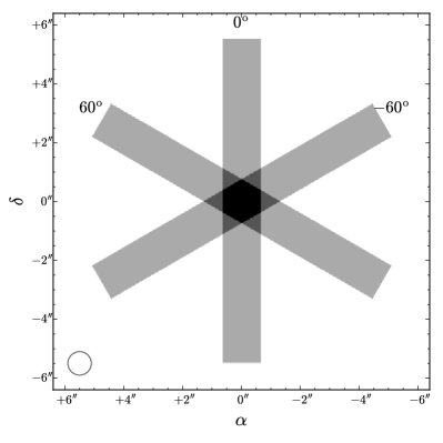
Figure 1: Effective exposure time map on the sky. The three individual slits are shown. Darker colour corresponds to higher effective exposure time. The circle in the lower left corner shows the average seeing disk of 0$\aas@@fstack{\prime\prime}$8.

2.1 Compilation of the Statistical Sample

The emission counterpart of PKS0458$-$020 was known from previous work (Moller2004) and included in our campaign as a sanity check in order to ensure that our spectroscopic setup is sensitive enough. Moreover, the new observations allow us to measure the Ly$\alpha$ flux at the position angle reported by Moller2004. Furthermore, the target Q0030$-$5129 was observed as a back-up target during one of the observing runs (088.A-0101). The DLA towards Q0030–5129 does not meet the line-strength criterion and consequently does not meet the metallicity requirement (Hartoog2015). Lastly, we notice that there are two DLAs towards Q2348–011. The second of these two DLAs (at $z_{\rm DLA}=2.614$) does not meet the line-strength criterion (with a $W_{\rm rest}$ of Si ii$\,\lambda 1526$ of only 0.4 Å). Since those three DLAs have not been selected in the same way as the rest of our sample (i.e., one was known already and the other two did not meet our metal line-strength criterion), these targets are excluded from our statistical analyses. We thus have a final statistical sample of 11 DLAs. The three targets mentioned above are included in this work for completeness.

2.2 Spectroscopic Observations

For the spectroscopic observations, we have used the X-shooter instrument, which is mounted on unit 2 of the Very Large Telescope at Paranal observatory in Chile operated by the European Southern Observatory. The spectrograph covers the observed wavelength range from $3000$ Å to $2.5~{}\mu$m simultaneously by splitting the light into three separate spectrographs, the so-called ‘arms’: UVB ($3000-5500$ Å), VIS ($5500-10000$ Å), and NIR ($10000-25000$ Å).

The main strategy of the campaign is presented in Fynbo2010, and we will only briefly summarize the main points of the spectroscopic setup. Each quasar is observed using long-slit spectroscopy at three position angles (PA1=$0$°, PA2=$+60$°, and PA3=$-60$°east of north) in order to cover as much of the region around the quasar as possible. These three position angles are referred to as PA1, PA2, and PA3, respectively. All observations are carried out using the same slit widths of 1$\aas@@fstack{\prime\prime}$3, 1$\aas@@fstack{\prime\prime}$2 and 1$\aas@@fstack{\prime\prime}$2 for UVB, VIS and NIR, respectively. All slits have the same length of 11″. The effective slit configuration is shown schematically in Fig. 1. An overview of the sample, including information regarding the observations, is provided in Table 1.

2.3 Data Reduction

For seven quasars, PKS0458–020, Q0316+0040, Q0338$-$0005, Q2348$-$011, Q0845+2008, Q1435+0354, and Q1313+1441, the data are published here for the first time. The data processing of these seven quasars is described in the following section. The raw data frames are first corrected for cosmic ray hits using the code DCR (DCR). The spectra are subsequently reduced using the official X-shooter pipeline version 2.5 for ‘stare mode’. The pipeline performs the following steps for each arm independently: First, the raw frames are corrected for the bias level (UVB and VIS) and dark current (NIR). Then the background is subtracted followed by a subtraction of the sky emission lines using the method laid out by Kelson03. After division by the spectral flat-field, the individual orders are extracted and rectified in wavelength space. The individual orders are then merged using error weighting in the overlapping regions. The resulting spectrum is a merged 2-dimensional spectrum and its error spectrum. Intermediate products such as the sky spectrum and individual echelle orders (with errors and bad-pixel maps) are also produced. From the 2-dimensional spectrum, we extract a 1-dimensional spectrum using our own python implementation of the optimal extraction algorithm (Horne1986). The 1-dimensional spectrum is subsequently converted to vacuum wavelengths and shifted to the helio-centric rest-frame. No correction of telluric absorption has been performed.

The relative flux calibration performed by the X-shooter pipeline provides a robust recovery of the spectral shape (to within 5%, measured from our spectra by comparing to photometry); however, in order to improve the absolute flux calibration, we have scaled our spectra to their corresponding photometry from SDSS. We scale the UVB arm in order to obtain the most precise flux calibration for the Ly$\alpha$ emission detections and match the VIS arm to the calibration achieved in the UVB. For this purpose, we use the $g$-band from SDSS as this band is more robust than the $u$-band. Since the quasars could have undergone intrinsic variations in their luminosities between our spectroscopic observations and the epoch of observation by the SDSS (of the order $\sim$10 to 15%; Giveon1999), we assign a conservative uncertainty on the flux calibration of 15%. One target is not covered by the SDSS footprint, namely PKS0458–020. For this target, we use instead observations from Souchay2012 in the Johnson $B$-band ($B_{J}=19.1\pm 0.1$) to calibrate the UVB arm. The flux calibration for this target is much less reliable due to the worse quality of photometric data available. The large uncertainty has been taken into account in the analysis of this target.

In order to study the absorption lines from the DLAs in greater detail, we combine the three 1-dimensional spectra for each target (corresponding to each position angle) using the error spectra as weights for the combination and masking bad pixels in individual spectra. For Q1313+1441, we observe a small shift in wavelengths between the UVB and VIS arms of 0.6 Å (3 pixels in the UVB arm, corresponding to roughly one third of the used slit-width) due to uncertainties in the wavelength calibration and centring of the object in the three slits. Similar offsets have been noted previously for X-shooter. We have subsequently shifted the UVB spectrum to match the VIS wavelength calibration.

As mentioned, the seeing was smaller than the used slit-widths. This affects not only the wavelength calibration but also the determination of the resolution, $\mathcal{R}$, as the instrument specific values are no longer valid. To overcome this, we infer the resolving power of each spectrum by convolving a telluric absorption template with a Gaussian kernel to match the observed telluric profiles. In order not to blur the telluric lines, the resolving power was inferred from a separate combination of the spectra before applying the air-to-vacuum conversion and the correction for the relative motion of the observatory relative to the helio-centric frame. Since we mainly fit absorption lines in the VIS arm, we only report the spectral resolution for this arm, the obtained values are given in Appendix LABEL:app:fits. For one case (Q1313+1441) we also fit transitions in the UVB arm. We therefore determine the resolving power by using the seeing as an estimate of the effective slit width. We then interpolate between the tabulated values of resolution for given slit widths (assuming an inverse proportionality between $\mathcal{R}$ and slit width). Using the average seeing in the $V$-band, we infer a resolution in the UVB arm of 8000.

Table 1: X-shooter observing log

Target	R.A.	Decl.	P.A.${}^{(a)}$	Exp. time	Date	Airmass${}^{(b)}$	Seeing${}^{(b)}$	Prog. ID	Reference
				(sec)			(arcsec)
Q0030–5129	00:30:34.37	$-$51:29:46.3	$0$°	3600	2011-10-21	1.13	0.78	088.A-0601	(8)
			$+60$°	3600	2011-10-21	1.21	1.00	088.A-0601
			$-60$°	3600	2011-10-21	1.37	0.90	088.A-0601
Q0316+0040	03:16:09.75	$+$00:40:42.6	$0$°	3200	2010-11-09	1.17	0.53	086.A-0074
			$+60$°	3200	2010-11-09	1.11	0.78	086.A-0074
			$-60$°	3200	2010-11-09	1.13	0.56	086.A-0074
Q0338–0005	03:38:54.74	$-$00:05:21.3	$0$°	3200	2010-11-09	1.18	0.71	086.A-0074	(5)
			$+60$°	3200	2010-11-09	1.36	0.53	086.A-0074
			$-60$°	3200	2010-11-09	1.75	0.56	086.A-0074
PKS0458–020	05:01:12.77	$-$01:59:14.8	$-60.4$°	3600	2010-02-16	1.40	1.86	084.A-0303	(1,5,9)
Q0845+2008	08:45:02.85	$+$20:08:50.7	$0$°	3600	2012-04-19	1.48	0.68	089.A-0068
			$+60$°	3600	2012-04-20	1.75	0.69	089.A-0068
			$-60$°	3600	2012-04-21	1.64	0.72	089.A-0068
Q0918+1636	09:18:26.16	$+$16:36:09.0	$0$°	3600	2010-02-16	1.43	0.70	084.A-0303	(4,7)
			$+60$°	3600	2010-02-16	1.34	0.71	084.A-0303
			$-60$°	3600	2010-02-16	1.40	0.65	084.A-0303
Q1057+0629	10:57:44.45	$+$06:29:14.5	$0$°	3600	2010-03-19	1.35	0.71	084.A-0524	(8)
			$+60$°	3600	2010-03-19	1.20	0.57	084.A-0524
			$-60$°	3600	2010-03-19	1.20	0.50	084.A-0524
Q1313+1441	13:13:41.17	$+$14:41:40.4	$0$°	3600	2012-04-20	1.34	0.61	089.A-0068
			$+60$°	3600	2012-04-20	1.29	0.74	089.A-0068
			$-60$°	3600	2012-04-21	1.41	0.86	089.A-0068
Q1435+0354	14:35:00.22	$+$03:54:03.7	$0$°	3600	2012-04-21	1.24	0.91	089.A-0068
			$+60$°	3600	2012-04-21	1.15	0.97	089.A-0068
			$-60$°	1100	2012-04-20	1.16	0.64	089.A-0068
Q2059–0528	20:59:22.43	$-$05:28:42.8	$0$°	3600	2011-10-20	1.09	0.74	088.A-0601	(8)
			$+60$°	3600	2011-10-21	1.21	1.24	088.A-0601
			$-60$°	3600	2011-10-21	1.50	1.24	088.A-0601
Q2222–0946${}^{(c)}$	22:22:56.11	$-$09:46:36.2	$0$°	3600	2009-10-21	1.06	1.05	084.A-0303	(3,6)
			$0$°	3600	2009-10-22	1.05	1.15	084.A-0303
			$-60$°	3600	2009-10-22	1.16	1.35	084.A-0303
Q2348–011	23:50:57.82	$-$00:52:09.8	$0$°	3200	2010-11-09	1.09	0.84	086.A-0074	(2)
			$+60$°	3200	2010-11-09	1.15	0.58	086.A-0074
			$-60$°	3600	2010-11-10	1.09	0.93	086.A-0074

${}^{(a)}$ Position angle of the slit measured East of North.

${}^{(b)}$ Airmass and seeing is averaged over the exposure.

${}^{(c)}$ Due to an error in the execution of our observations at the telescope, the object was observed twice at ${\rm PA}=0$° and once at ${\rm PA}=-60$°.
${}^{(c)}$ Hence, we did not get a spectrum at ${\rm PA}=+60$°.

References: (1) Moller2004; (2) Noterdaeme2007; (3) Fynbo2010; (4) Fynbo2011; (5) Krogager2012;
References: (6) Krogager2013; (7) Fynbo2013b; (8) Hartoog2015; (9) Ledoux2006.

3 Analysis of X-shooter data

3.1 Absorption Lines

The column densities of H i and low-ionization metal lines have been obtained through Voigt-profile fitting using our own python code (see Appendix A of Krogager_PhD). We search the spectra for suitable transitions of Fe ii, Si ii, Zn ii, Cr ii, and S ii, however, not all species are available for all the DLAs. Under the assumption that the low-ionization lines arise from similar conditions in the absorbing medium, we fit all the lines from the singly ionized state using the same velocity structure, i.e., the number of components, relative velocities, and line broadening parameters are tied for all species. The DLA at $z_{\textsc{dla}}=2.425$ toward Q2348$-$011 has been analysed previously by Noterdaeme2007. For the species covered by the analysis of Noterdaeme et al. (Fe ii, Si ii, and S ii), we use their measured values as the high-resolution data from UVES provide a better fit (though we obtain consistent values from our fits). The metallicities obtained from the absorption line analysis are listed in Table 2 together with values for the previously analysed DLAs in the sample (these are marked with a number pointing to the reference, from which the measurement was taken). The fitted transitions and the best-fit profiles are shown in Appendix LABEL:app:fits. For the DLA at $z_{\textsc{dla}}=2.229$ towards Q0338$-$0005, we note that a previous measurement of [Si/H] $=-1.22\pm 0.11$ has been published using high-resolution data from UVES (Jorgenson2013). Although the UVES data have higher spectral resolution, the X-shooter data presented here have a much higher signal-to-noise ratio. We therefore use the measured quantity from this work over the one measured from the UVES data. The comparison of the two datasets is shown in Fig. 2.

For the target Q1313+1441, we fitted the available transitions (Si ii, Zn ii, Fe ii, Cr ii, and Mg i) in the VIS and UVB arms separately. Since the velocity structure of Mg i is consistent with the observed structure for the singly ionized species, we tied the relative velocities and broadening parameters of the Mg i line to the singly ionized species (Fe ii, Zn ii, and Cr ii). For the Si ii $\lambda 1808$ line in the UVB arm, we then used the same velocity structure derived from the higher resolution data in the VIS arm to fit the Si ii line while only allowing the column density to vary.

We measure the velocity width of the absorption lines, $\Delta V_{90}$, following the definition by Prochaska1997. For this purpose, we select weak, unblended low-ionization transitions in the VIS spectra. We deconvolve the measured $\Delta V_{90}$ using equation 1 from Arabsalmani2015. The deconvolved velocity widths are given in Table 2.

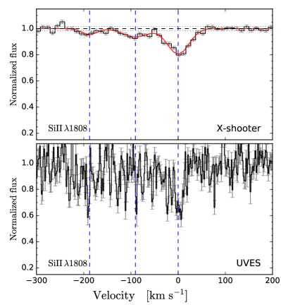
Figure 2: Comparison of the Si ii$\lambda\,1808$ line for the DLA toward the quasar Q0338$-$0005 presented in this work (top panel) and the UVES data of the same transition (lower panel). The red solid line in the top panel indicates the best-fit model from our Voigt-profile analysis. The improved signal-to-noise ratio in the top panel is evident and the broad velocity structure is clearly seen in the X-shooter data. The UVES data shown here have been obtained from the ESO archive of science-grade, pipeline-processed data products.

Table 2: Absorption properties of the X-shooter campaign.

Target	$z_{\textsc{dla}}$	$\log(N_{\rm H\,\textsc{i}}/{\rm cm}^{-2})$	[Zn/H]	[Si/H]	[Fe/H]	[Cr/H]	[S/H]	$\Delta V_{90}\,^{(a)}$
Q0030–5129	2.452	$20.8 \pm 0.2^{(7)}$	$-1.48\pm 0.34^{(7)}$	–	$-1.55\pm 0.20^{(7)}$	$-1.57\pm 0.27^{(7)}$	–	41
Q0316+0040	2.179	$21.04\pm 0.05$	$-1.02\pm 0.07$	$-0.95\pm 0.06$	$-1.45\pm 0.06$	$-1.17\pm 0.06$	–	69
Q0338–0005	2.229	$21.12\pm 0.05$	$-1.36\pm 0.07$	$-1.36\pm 0.06$	–	$-1.46\pm 0.06$	–	221
PKS0458–020	2.040	$21.70\pm 0.10^{(1)}$	$-1.22\pm 0.10^{(1)}$	–	–	–	–	87${}^{(1)}$
Q0845+2008	2.237	$20.41\pm 0.06$	$+0.05\pm 0.08$	$-0.29\pm 0.07$	$<-0.8\pm 0.1$	$-0.79\pm 0.07$	–	155
Q0918+1636-1	2.412	$21.26\pm 0.06^{(5)}$	$-0.6\pm 0.2^{(5)}$	$-0.6\pm 0.2^{(5)}$	$-1.2\pm 0.2^{(5)}$	$-1.2\pm 0.2^{(5)}$	–	350${}^{(5)}$
Q0918+1636-2	2.583	$20.96\pm 0.05^{(4)}$	$-0.12\pm 0.05^{(4)}$	$-0.46\pm 0.05^{(4)}$	$-1.03\pm 0.05^{(4)}$	$-0.88\pm 0.05^{(4)}$	$-0.26\pm 0.05^{(4)}$	293${}^{(4)}$
Q1057+0629	2.499	$20.51\pm 0.03^{(7)}$	$-0.24\pm 0.11^{(7)}$	$-0.37\pm 0.05^{(7)}$	$-0.98\pm 0.03^{(7)}$	–	$-0.15\pm 0.06^{(7)}$	328
Q1313+1441	1.794	$21.3\pm 0.1$	$-0.7\pm 0.1$	$-0.8\pm 0.1$	$-1.5\pm 0.1$	$-1.2\pm 0.1$	–	164
Q1435+0354	2.269	$20.42\pm 0.08$	$-0.4\pm 0.1$	$-0.6\pm 0.1$	$-1.1\pm 0.1$	$-0.7\pm 0.1$	–	183
Q2059–0528	2.210	$21.00\pm 0.05^{(7)}$	$-0.96\pm 0.06^{(7)}$	$-0.99\pm 0.05^{(7)}$	$-1.41\pm 0.05^{(7)}$	$-1.19\pm 0.05^{(7)}$	$-0.91\pm 0.06^{(7)}$	114${}^{(7)}$
Q2222–0946	2.354	$20.65\pm 0.05^{(6)}$	$-0.38\pm 0.05^{(6)}$	$-0.54\pm 0.05^{(6)}$	$-1.02\pm 0.05^{(6)}$	–	$-0.49\pm 0.05^{(6)}$	181${}^{(3)}$
Q2348–011-1	2.425	$20.53\pm 0.06$	$-0.33\pm 0.08$	$-0.80\pm 0.10^{(2)}$	$-1.17\pm 0.10^{(2)}$	$-1.25\pm 0.07$	$-0.62\pm 0.10^{(2)}$	240
Q2348–011-2	2.614	$21.34\pm 0.06$	–	$-1.98\pm 0.08$	$-2.46\pm 0.08$	$-2.13\pm 0.08$	–	63

${}^{(a)}$ $\Delta V_{90}$ in units of km s${}^{-1}$, corrected for resolution effects following Arabsalmani2015.
${}^{(a)}$ Typical uncertainties on $\Delta V_{90}$ are of the order 10–20 km s${}^{-1}$. Si ii $\lambda 1808$ was used in all cases except for Q1313+1441, where Cr ii $\lambda 2056$ was used.

References: (1) Ledoux2006; (2) Noterdaeme2007; (3) Fynbo2010; (4) Fynbo2011; (5) Fynbo2013b;
References: (6) Krogager2013; (7) Hartoog2015.