SphereFace: Deep Hypersphere Embedding for Face Recognition
Abstract
This paper addresses deep face recognition (FR) problem under open-set protocol, where ideal face features are expected to have smaller maximal intra-class distance than minimal inter-class distance under a suitably chosen metric space. However, few existing algorithms can effectively achieve this criterion. To this end, we propose the angular softmax (A-Softmax) loss that enables convolutional neural networks (CNNs) to learn angularly discriminative features. Geometrically, A-Softmax loss can be viewed as imposing discriminative constraints on a hypersphere manifold, which intrinsically matches the prior that faces also lie on a manifold. Moreover, the size of angular margin can be quantitatively adjusted by a parameter . We further derive specific to approximate the ideal feature criterion. Extensive analysis and experiments on Labeled Face in the Wild (LFW), Youtube Faces (YTF) and MegaFace Challenge show the superiority of A-Softmax loss in FR tasks. The code has also been made publicly available111See the code at https://github.com/wy1iu/sphereface..
1 Introduction
Recent years have witnessed the great success of convolutional neural networks (CNNs) in face recognition (FR). Owing to advanced network architectures [13, 23, 29, 4] and discriminative learning approaches [25, 22, 34], deep CNNs have boosted the FR performance to an unprecedent level. Typically, face recognition can be categorized as face identification and face verification [8, 11]. The former classifies a face to a specific identity, while the latter determines whether a pair of faces belongs to the same identity.
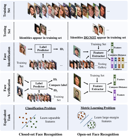
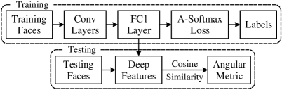
In terms of testing protocol, face recognition can be evaluated under closed-set or open-set settings, as illustrated in Fig. 1. For closed-set protocol, all testing identities are predefined in training set. It is natural to classify testing face images to the given identities. In this scenario, face verification is equivalent to performing identification for a pair of faces respectively (see left side of Fig. 1). Therefore, closed-set FR can be well addressed as a classification problem, where features are expected to be separable. For open-set protocol, the testing identities are usually disjoint from the training set, which makes FR more challenging yet close to practice. Since it is impossible to classify faces to known identities in training set, we need to map faces to a discriminative feature space. In this scenario, face identification can be viewed as performing face verification between the probe face and every identity in the gallery (see right side of Fig. 1). Open-set FR is essentially a metric learning problem, where the key is to learn discriminative large-margin features.
Desired features for open-set FR are expected to satisfy the criterion that the maximal intra-class distance is smaller than the minimal inter-class distance under a certain metric space. This criterion is necessary if we want to achieve perfect accuracy using nearest neighbor. However, learning features with this criterion is generally difficult because of the intrinsically large intra-class variation and high inter-class similarity [21] that faces exhibit.
Few CNN-based approaches are able to effectively formulate the aforementioned criterion in loss functions. Pioneering work [30, 26] learn face features via the softmax loss222Following [16], we define the softmax loss as the combination of the last fully connected layer, softmax function and cross-entropy loss., but softmax loss only learns separable features that are not discriminative enough. To address this, some methods combine softmax loss with contrastive loss [25, 28] or center loss [34] to enhance the discrimination power of features. [22] adopts triplet loss to supervise the embedding learning, leading to state-of-the-art face recognition results. However, center loss only explicitly encourages intra-class compactness. Both contrastive loss [3] and triplet loss [22] can not constrain on each individual sample, and thus require carefully designed pair/triplet mining procedure, which is both time-consuming and performance-sensitive.
It seems to be a widely recognized choice to impose Euclidean margin to learned features, but a question arises: Is Euclidean margin always suitable for learning discriminative face features? To answer this question, we first look into how Euclidean margin based losses are applied to FR.
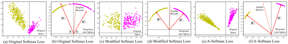
Most recent approaches [25, 28, 34] combine Euclidean margin based losses with softmax loss to construct a joint supervision. However, as can be observed from Fig. 2, the features learned by softmax loss have intrinsic angular distribution (also verified by [34]). In some sense, Euclidean margin based losses are incompatible with softmax loss, so it is not well motivated to combine these two type of losses.
In this paper, we propose to incorporate angular margin instead. We start with a binary-class case to analyze the softmax loss. The decision boundary in softmax loss is , where and are weights and bias333If not specified, the weights and biases in the paper are corresponding to the fully connected layer in the softmax loss. in softmax loss, respectively. If we define as a feature vector and constrain and , the decision boundary becomes , where is the angle between and . The new decision boundary only depends on and . Modified softmax loss is able to directly optimize angles, enabling CNNs to learn angularly distributed features (Fig. 2).
Compared to original softmax loss, the features learned by modified softmax loss are angularly distributed, but not necessarily more discriminative. To the end, we generalize the modified softmax loss to angular softmax (A-Softmax) loss. Specifically, we introduce an integer () to quantitatively control the decision boundary. In binary-class case, the decision boundaries for class 1 and class 2 become and , respectively. quantitatively controls the size of angular margin. Furthermore, A-Softmax loss can be easily generalized to multiple classes, similar to softmax loss. By optimizing A-Softmax loss, the decision regions become more separated, simultaneously enlarging the inter-class margin and compressing the intra-class angular distribution.
A-Softmax loss has clear geometric interpretation. Supervised by A-Softmax loss, the learned features construct a discriminative angular distance metric that is equivalent to geodesic distance on a hypersphere manifold. A-Softmax loss can be interpreted as constraining learned features to be discriminative on a hypersphere manifold, which intrinsically matches the prior that face images lie on a manifold [14, 5, 31]. The close connection between A-Softmax loss and hypersphere manifolds makes the learned features more effective for face recognition. For this reason, we term the learned features as SphereFace.
Moreover, A-Softmax loss can quantitatively adjust the angular margin via a parameter , enabling us to do quantitative analysis. In the light of this, we derive lower bounds for the parameter to approximate the desired open-set FR criterion that the maximal intra-class distance should be smaller than the minimal inter-class distance.
Our major contributions can be summarized as follows:
(1) We propose A-Softmax loss for CNNs to learn discriminative face features with clear and novel geometric interpretation. The learned features discriminatively span on a hypersphere manifold, which intrinsically matches the prior that faces also lie on a manifold.
(2) We derive lower bounds for such that A-Softmax loss can approximate the learning task that minimal inter-class distance is larger than maximal intra-class distance.
(3) We are the very first to show the effectiveness of angular margin in FR. Trained on publicly available CASIA dataset [37], SphereFace achieves competitive results on several benchmarks, including Labeled Face in the Wild (LFW), Youtube Faces (YTF) and MegaFace Challenge 1.
2 Related Work
Metric learning. Metric learning aims to learn a similarity (distance) function. Traditional metric learning [36, 33, 12, 38] usually learns a matrix for a distance metric upon the given features . Recently, prevailing deep metric learning [7, 17, 24, 30, 25, 22, 34] usually uses neural networks to automatically learn discriminative features followed by a simple distance metric such as Euclidean distance . Most widely used loss functions for deep metric learning are contrastive loss [1, 3] and triplet loss [32, 22, 6], and both impose Euclidean margin to features.
Deep face recognition. Deep face recognition is arguably one of the most active research area in the past few years. [30, 26] address the open-set FR using CNNs supervised by softmax loss, which essentially treats open-set FR as a multi-class classification problem. [25] combines contrastive loss and softmax loss to jointly supervise the CNN training, greatly boosting the performance. [22] uses triplet loss to learn a unified face embedding. Training on nearly 200 million face images, they achieve current state-of-the-art FR accuracy. Inspired by linear discriminant analysis, [34] proposes center loss for CNNs and also obtains promising performance. In general, current well-performing CNNs [28, 15] for FR are mostly built on either contrastive loss or triplet loss. One could notice that state-of-the-art FR methods usually adopt ideas (e.g. contrastive loss, triplet loss) from metric learning, showing open-set FR could be well addressed by discriminative metric learning.
L-Softmax loss [16] also implicitly involves the concept of angles. As a regularization method, it shows great improvement on closed-set classification problems. Differently, A-Softmax loss is developed to learn discriminative face embedding. The explicit connections to hypersphere manifold makes our learned features particularly suitable for open-set FR problem, as verified by our experiments. In addition, the angular margin in A-Softmax loss is explicitly imposed and can be quantitatively controlled (e.g. lower bounds to approximate desired feature criterion), while [16] can only be analyzed qualitatively.
3 Deep Hypersphere Embedding
3.1 Revisiting the Softmax Loss
We revisit the softmax loss by looking into the decision criteria of softmax loss. In binary-class case, the posterior probabilities obtained by softmax loss are
| (1) |
| (2) |
where is the learned feature vector. and are weights and bias of last fully connected layer corresponding to class , respectively. The predicted label will be assigned to class 1 if and class 2 if . By comparing and , it is clear that and determine the classification result. The decision boundary is . We then rewrite as where is the angle between and . Notice that if we normalize the weights and zero the biases (, ), the posterior probabilities become and . Note that and share the same , the final result only depends on the angles and . The decision boundary also becomes (i.e. angular bisector of vector and ). Although the above analysis is built on binary-calss case, it is trivial to generalize the analysis to multi-class case. During training, the modified softmax loss () encourages features from the -th class to have smaller angle (larger cosine distance) than others, which makes angles between and features a reliable metric for classification.
To give a formal expression for the modified softmax loss, we first define the input feature and its label . The original softmax loss can be written as
| (3) |
where denotes the -th element (, is the class number) of the class score vector , and is the number of training samples. In CNNs, is usually the output of a fully connected layer , so and where , are the -th training sample, the -th and -th column of respectively. We further reformulate in Eq. (3) as
| (4) | ||||
in which is the angle between vector and . As analyzed above, we first normalize in each iteration and zero the biases. Then we have the modified softmax loss:
| (5) |
Although we can learn features with angular boundary with the modified softmax loss, these features are still not necessarily discriminative. Since we use angles as the distance metric, it is natural to incorporate angular margin to learned features in order to enhance the discrimination power. To this end, we propose a novel way to combine angular margin.
3.2 Introducing Angular Margin to Softmax Loss
Instead of designing a new type of loss function and constructing a weighted combination with softmax loss (similar to contrastive loss) , we propose a more natural way to learn angular margin. From the previous analysis of softmax loss, we learn that decision boundaries can greatly affect the feature distribution, so our basic idea is to manipulate decision boundaries to produce angular margin. We first give a motivating binary-class example to explain how our idea works.
Assume a learned feature from class 1 is given and is the angle between and , it is known that the modified softmax loss requires to correctly classify . But what if we instead require where is a integer in order to correctly classify ? It is essentially making the decision more stringent than previous, because we require a lower bound444The inequality holds while . of to be larger than . The decision boundary for class 1 is . Similarly, if we require to correctly classify features from class 2, the decision boundary for class 2 is . Suppose all training samples are correctly classified, such decision boundaries will produce an angular margin of where is the angle between and . From angular perspective, correctly classifying from identity 1 requires , while correctly classifying from identity 2 requires . Both are more difficult than original and , respectively. By directly formulating this idea into the modified softmax loss Eq. (5), we have
| (6) |
where has to be in the range of . In order to get rid of this restriction and make it optimizable in CNNs, we expand the definition range of by generalizing it to a monotonically decreasing angle function which should be equal to in . Therefore, our proposed A-Softmax loss is formulated as:
| (7) |
in which we define , and . is an integer that controls the size of angular margin. When , it becomes the modified softmax loss.
| Loss Function | Decision Boundary | ||
|---|---|---|---|
| Softmax Loss | |||
| Modified Softmax Loss | |||
| A-Softmax Loss |
|
The justification of A-Softmax loss can also be made from decision boundary perspective. A-Softmax loss adopts different decision boundary for different class (each boundary is more stringent than the original), thus producing angular margin. The comparison of decision boundaries is given in Table 1. From original softmax loss to modified softmax loss, it is from optimizing inner product to optimizing angles. From modified softmax loss to A-Softmax loss, it makes the decision boundary more stringent and separated. The angular margin increases with larger and be zero if .
Supervised by A-Softmax loss, CNNs learn face features with geometrically interpretable angular margin. Because A-Softmax loss requires , it makes the prediction only depends on angles between the sample and . So can be classified to the identity with smallest angle. The parameter is added for the purpose of learning an angular margin between different identities.
To facilitate gradient computation and back propagation, we replace and with the expressions only containing and , which is easily done by definition of cosine and multi-angle formula (also the reason why we need to be an integer). Without , we can compute derivative with respect to and , similar to softmax loss.
3.3 Hypersphere Interpretation of A-Softmax Loss
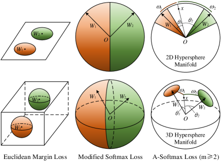
A-Softmax loss has stronger requirements for a correct classification when , which generates an angular classification margin between learned features of different classes. A-Softmax loss not only imposes discriminative power to the learned features via angular margin, but also renders nice and novel hypersphere interpretation. As shown in Fig. 3, A-Softmax loss is equivalent to learning features that are discriminative on a hypersphere manifold, while Euclidean margin losses learn features in Euclidean space.
To simplify, We take the binary case to analyze the hypersphere interpretation. Considering a sample from class 1 and two column weights , the classification rule for A-Softmax loss is , equivalently . Notice that are equal to their corresponding arc length 555 is the shortest arc length (geodesic distance) between and the projected point of sample on the unit hypersphere, while the corresponding is the angle between and . on unit hypersphere . Because , the decision replies on the arc length and . The decision boundary is equivalent to , and the constrained region for correctly classifying to class 1 is . Geometrically speaking, this is a hypercircle-like region lying on a hypersphere manifold. For example, it is a circle-like region on the unit sphere in 3D case, as illustrated in Fig. 3. Note that larger leads to smaller hypercircle-like region for each class, which is an explicit discriminative constraint on a manifold. For better understanding, Fig. 3 provides 2D and 3D visualizations. One can see that A-Softmax loss imposes arc length constraint on a unit circle in 2D case and circle-like region constraint on a unit sphere in 3D case. Our analysis shows that optimizing angles with A-Softmax loss essentially makes the learned features more discriminative on a hypersphere.
3.4 Properties of A-Softmax Loss
Property 1.
A-Softmax loss defines a large angular margin learning task with adjustable difficulty. With larger , the angular margin becomes larger, the constrained region on the manifold becomes smaller, and the corresponding learning task also becomes more difficult.
We know that the larger is, the larger angular margin A-Softmax loss constrains. There exists a minimal that constrains the maximal intra-class angular distance to be smaller than the minimal inter-class angular distance, which can also be observed in our experiments.
Definition 1 (minimal for desired feature distribution).
is the minimal value such that while , A-Softmax loss defines a learning task where the maximal intra-class angular feature distance is constrained to be smaller than the minimal inter-class angular feature distance.
Property 2 (lower bound of in binary-class case).
In binary-class case, we have .
Proof.
We consider the space spaned by and . Because , it is easy to obtain the maximal angle that class 1 spans is where is the angle between and . To require the maximal intra-class feature angular distance smaller than the minimal inter-class feature angular distance, we need to constrain
| (8) |
| (9) |
After solving these two inequalities, we could have , which is a lower bound for binary case. ∎
Property 3 (lower bound of in multi-class case).
Under the assumption that are uniformly spaced in the Euclidean space, we have .
Proof.
We consider the 2D -class () scenario for the lower bound. Because are uniformly spaced in the 2D Euclidean space, we have where is the angle between and . Since are symmetric, we only need to analyze one of them. For the -th class (), We need to constrain
| (10) |
After solving this inequality, we obtain , which is a lower bound for multi-class case. ∎
Based on this, we use to approximate the desired feature distribution criteria. Since the lower bounds are not necessarily tight, giving a tighter lower bound and a upper bound under certain conditions is also possible, which we leave to the future work. Experiments also show that larger consistently works better and will usually suffice.
3.5 Discussions
Why angular margin. First and most importantly, angular margin directly links to discriminativeness on a manifold, which intrinsically matches the prior that faces also lie on a manifold. Second, incorporating angular margin to softmax loss is actually a more natural choice. As Fig. 2 shows, features learned by the original softmax loss have an intrinsic angular distribution. So directly combining Euclidean margin constraints with softmax loss is not reasonable.
Comparison with existing losses. In deep FR task, the most popular and well-performing loss functions include contrastive loss, triplet loss and center loss. First, they only impose Euclidean margin to the learned features (w/o normalization), while ours instead directly considers angular margin which is naturally motivated. Second, both contrastive loss and triplet loss suffer from data expansion when constituting the pairs/triplets from the training set, while ours requires no sample mining and imposes discriminative constraints to the entire mini-batches (compared to contrastive and triplet loss that only affect a few representative pairs/triplets).
| Layer | 4-layer CNN | 10-layer CNN | 20-layer CNN | 36-layer CNN | 64-layer CNN | ||||||||
| Conv1.x | [33, 64]1, S2 | [33, 64]1, S2 |
|
|
|
||||||||
| Conv2.x | [33, 128]1, S2 |
|
|
|
|
||||||||
| Conv3.x | [33, 256]1, S2 |
|
|
|
|
||||||||
| Conv4.x | [33, 512]1, S2 | [33, 512]1, S2 |
|
|
|
||||||||
| FC1 | 512 | 512 | 512 | 512 | 512 |
4 Experiments (more in Appendix)
4.1 Experimental Settings
Preprocessing. We only use standard preprocessing. The face landmarks in all images are detected by MTCNN [39]. The cropped faces are obtained by similarity transformation. Each pixel () in RGB images is normalized by subtracting 127.5 and then being divided by 128.
CNNs Setup. Caffe [10] is used to implement A-Softmax loss and CNNs. The general framework to train and extract SphereFace features is shown in Fig. 4. We use residual units [4] in our CNN architecture. For fairness, all compared methods use the same CNN architecture (including residual units) as SphereFace. CNNs with different depths (4, 10, 20, 36, 64) are used to better evaluate our method. The specific settings for difffernt CNNs we used are given in Table 2. According to the analysis in Section 3.4, we usually set as 4 in A-Softmax loss unless specified. These models are trained with batch size of 128 on four GPUs. The learning rate begins with 0.1 and is divided by 10 at the 16K, 24K iterations. The training is finished at 28K iterations.
Training Data. We use publicly available web-collected training dataset CASIA-WebFace [37] (after excluding the images of identities appearing in testing sets) to train our CNN models. CASIA-WebFace has 494,414 face images belonging to 10,575 different individuals. These face images are horizontally flipped for data augmentation. Notice that the scale of our training data (0.49M) is relatively small, especially compared to other private datasets used in DeepFace [30] (4M), VGGFace [20] (2M) and FaceNet [22] (200M).
Testing. We extract the deep features (SphereFace) from the output of the FC1 layer. For all experiments, the final representation of a testing face is obtained by concatenating its original face features and its horizontally flipped features. The score (metric) is computed by the cosine distance of two features. The nearest neighbor classifier and thresholding are used for face identification and verification, respectively.
4.2 Exploratory Experiments
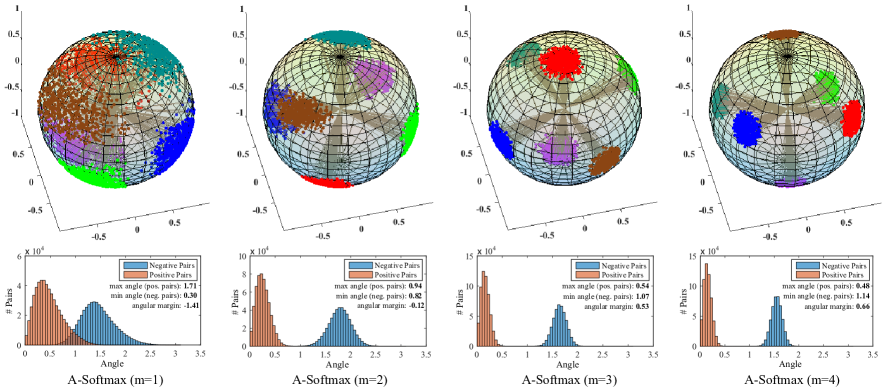
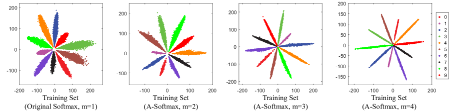
Effect of . To show that larger leads to larger angular margin (i.e. more discriminative feature distribution on manifold), we perform a toy example with different . We train A-Softmax loss with 6 individuals that have the most samples in CASIA-WebFace. We set the output feature dimension (FC1) as 3 and visualize the training samples in Fig. 5. One can observe that larger leads to more discriminative distribution on the sphere and also larger angular margin, as expected. We also use class 1 (blue) and class 2 (dark green) to construct positive and negative pairs to evaluate the angle distribution of features from the same class and different classes. The angle distribution of positive and negative pairs (the second row of Fig. 5) quantitatively shows the angular margin becomes larger while increases and every class also becomes more distinct with each other.
Besides visual comparison, we also perform face recognition on LFW and YTF to evaluate the effect of . For fair comparison, we use 64-layer CNN (Table 2) for all losses. Results are given in Table 3. One can observe that while becomes larger, the accuracy of A-Softmax loss also becomes better, which shows that larger angular margin can bring stronger discrimination power.
| Dataset | Original | m=1 | m=2 | m=3 | m=4 |
|---|---|---|---|---|---|
| LFW | 97.88 | 97.90 | 98.40 | 99.25 | 99.42 |
| YTF | 93.1 | 93.2 | 93.8 | 94.4 | 95.0 |
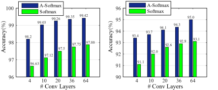
Effect of CNN architectures. We train A-Softmax loss () and original softmax loss with different number of convolution layers. Specific CNN architectures can be found in Table 2. From Fig. 6, one can observe that A-Softmax loss consistently outperforms CNNs with softmax loss (1.54%1.91%), indicating that A-Softmax loss is more suitable for open-set FR. Besides, the difficult learning task defined by A-Softmax loss makes full use of the superior learning capability of deeper architectures. A-Softmax loss greatly improve the verification accuracy from 98.20% to 99.42% on LFW, and from 93.4% to 95.0% on YTF. On the contrary, the improvement of deeper standard CNNs is unsatisfactory and also easily get saturated (from 96.60% to 97.75% on LFW, from 91.1% to 93.1% on YTF).
4.3 Experiments on LFW and YTF
| Method | Models | Data | LFW | YTF |
|---|---|---|---|---|
| DeepFace [30] | 3 | 4M* | 97.35 | 91.4 |
| FaceNet [22] | 1 | 200M* | 99.65 | 95.1 |
| Deep FR [20] | 1 | 2.6M | 98.95 | 97.3 |
| DeepID2+ [27] | 1 | 300K* | 98.70 | N/A |
| DeepID2+ [27] | 25 | 300K* | 99.47 | 93.2 |
| Baidu [15] | 1 | 1.3M* | 99.13 | N/A |
| Center Face [34] | 1 | 0.7M* | 99.28 | 94.9 |
| Yi et al. [37] | 1 | WebFace | 97.73 | 92.2 |
| Ding et al. [2] | 1 | WebFace | 98.43 | N/A |
| Liu et al. [16] | 1 | WebFace | 98.71 | N/A |
| Softmax Loss | 1 | WebFace | 97.88 | 93.1 |
| Softmax+Contrastive [26] | 1 | WebFace | 98.78 | 93.5 |
| Triplet Loss [22] | 1 | WebFace | 98.70 | 93.4 |
| L-Softmax Loss [16] | 1 | WebFace | 99.10 | 94.0 |
| Softmax+Center Loss [34] | 1 | WebFace | 99.05 | 94.4 |
| SphereFace | 1 | WebFace | 99.42 | 95.0 |
LFW dataset [9] includes 13,233 face images from 5749 different identities, and YTF dataset [35] includes 3,424 videos from 1,595 different individuals. Both datasets contains faces with large variations in pose, expression and illuminations. We follow the unrestricted with labeled outside data protocol [8] on both datasets. The performance of SphereFace are evaluated on 6,000 face pairs from LFW and 5,000 video pairs from YTF. The results are given in Table 4. For contrastive loss and center loss, we follow the FR convention to form a weighted combination with softmax loss. The weights are selected via cross validation on training set. For L-Softmax [16], we also use . All the compared loss functions share the same 64-layer CNN architecture.
Most of the existing face verification systems achieve high performance with huge training data or model ensemble. While using single model trained on publicly available dataset (CAISA-WebFace, relatively small and having noisy labels), SphereFace achieves 99.42% and 95.0% accuracies on LFW and YTF datasets. It is the current best performance trained on WebFace and considerably better than the other models trained on the same dataset. Compared with models trained on high-quality private datasets, SphereFace is still very competitive, outperforming most of the existing results in Table 4. One should notice that our single model performance is only worse than Google FaceNet which is trained with more than 200 million data.
For fair comparison, we also implement the softmax loss, contrastive loss, center loss, triplet loss, L-Softmax loss [16] and train them with the same 64-layer CNN architecture as A-Softmax loss. As can be observed in Table 4, SphereFace consistently outperforms the features learned by all these compared losses, showing its superiority in FR tasks.
4.4 Experiments on MegaFace Challenge
| Method | protocol | Rank1 Acc. | Ver. |
|---|---|---|---|
| NTechLAB - facenx large | Large | 73.300 | 85.081 |
| Vocord - DeepVo1 | Large | 75.127 | 67.318 |
| Deepsense - Large | Large | 74.799 | 87.764 |
| Shanghai Tech | Large | 74.049 | 86.369 |
| Google - FaceNet v8 | Large | 70.496 | 86.473 |
| Beijing FaceAll_Norm_1600 | Large | 64.804 | 67.118 |
| Beijing FaceAll_1600 | Large | 63.977 | 63.960 |
| Deepsense - Small | Small | 70.983 | 82.851 |
| SIAT_MMLAB | Small | 65.233 | 76.720 |
| Barebones FR - cnn | Small | 59.363 | 59.036 |
| NTechLAB - facenx_small | Small | 58.218 | 66.366 |
| 3DiVi Company - tdvm6 | Small | 33.705 | 36.927 |
| Softmax Loss | Small | 54.855 | 65.925 |
| Softmax+Contrastive Loss [26] | Small | 65.219 | 78.865 |
| Triplet Loss [22] | Small | 64.797 | 78.322 |
| L-Softmax Loss [16] | Small | 67.128 | 80.423 |
| Softmax+Center Loss [34] | Small | 65.494 | 80.146 |
| SphereFace (single model) | Small | 72.729 | 85.561 |
| SphereFace (3-patch ensemble) | Small | 75.766 | 89.142 |
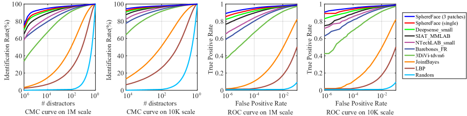
MegaFace dataset [18] is a recently released testing benchmark with very challenging task to evaluate the performance of face recognition methods at the million scale of distractors. MegaFace dataset contains a gallery set and a probe set. The gallery set contains more than 1 million images from 690K different individuals. The probe set consists of two existing datasets: Facescrub [19] and FGNet. MegaFace has several testing scenarios including identification, verification and pose invariance under two protocols (large or small training set). The training set is viewed as small if it is less than 0.5M. We evaluate SphereFace under the small training set protocol. We adopt two testing protocols: face identification and verification. The results are given in Fig. 7 and Tabel 5. Note that we use simple 3-patch feature concatenation ensemble as the final performance of SphereFace.
Fig. 7 and Tabel 5 show that SphereFace (3 patches ensemble) beats the second best result by a large margins (4.8% for rank-1 identification rate and 6.3% for verification rate) on MegaFace benchmark under the small training dataset protocol. Compared to the models trained on large dataset (500 million for Google and 18 million for NTechLAB), our method still performs better (0.64% for id. rate and 1.4% for veri. rate). Moreover, in contrast to their sophisticated network design, we only employ typical CNN architecture supervised by A-Softamx to achieve such excellent performance. For single model SphereFace, the accuracy of face identification and verification are still 72.73% and 85.56% respectively, which already outperforms most state-of-the-art methods. For better evaluation, we also implement the softmax loss, contrastive loss, center loss, triplet loss and L-Softmax loss [16]. Compared to these loss functions trained with the same CNN architecture and dataset, SphereFace also shows significant and consistent improvements. These results convincingly demonstrate that the proposed SphereFace is well designed for open-set face recognition. One can also see that learning features with large inter-class angular margin can significantly improve the open-set FR performance.
5 Concluding Remarks
This paper presents a novel deep hypersphere embedding approach for face recognition. In specific, we propose the angular softmax loss for CNNs to learn discriminative face features (SphereFace) with angular margin. A-Softmax loss renders nice geometric interpretation by constraining learned features to be discriminative on a hypersphere manifold, which intrinsically matches the prior that faces also lie on a non-linear manifold. This connection makes A-Softmax very effective for learning face representation. Competitive results on several popular face benchmarks demonstrate the superiority and great potentials of our approach. We also believe A-Softmax loss could also benefit some other tasks like object recognition, person re-identification, etc.
References
- [1] S. Chopra, R. Hadsell, and Y. LeCun. Learning a similarity metric discriminatively, with application to face verification. In CVPR, 2005.
- [2] C. Ding and D. Tao. Robust face recognition via multimodal deep face representation. IEEE TMM, 17(11):2049–2058, 2015.
- [3] R. Hadsell, S. Chopra, and Y. LeCun. Dimensionality reduction by learning an invariant mapping. In CVPR, 2006.
- [4] K. He, X. Zhang, S. Ren, and J. Sun. Deep residual learning for image recognition. In CVPR, 2016.
- [5] X. He, S. Yan, Y. Hu, P. Niyogi, and H.-J. Zhang. Face recognition using laplacianfaces. TPAMI, 27(3):328–340, 2005.
- [6] E. Hoffer and N. Ailon. Deep metric learning using triplet network. arXiv preprint:1412.6622, 2014.
- [7] J. Hu, J. Lu, and Y.-P. Tan. Discriminative deep metric learning for face verification in the wild. In CVPR, 2014.
- [8] G. B. Huang and E. Learned-Miller. Labeled faces in the wild: Updates and new reporting procedures. Dept. Comput. Sci., Univ. Massachusetts Amherst, Amherst, MA, USA, Tech. Rep, pages 14–003, 2014.
- [9] G. B. Huang, M. Ramesh, T. Berg, and E. Learned-Miller. Labeled faces in the wild: A database for studying face recognition in unconstrained environments. Technical report, Technical Report, 2007.
- [10] Y. Jia, E. Shelhamer, J. Donahue, S. Karayev, J. Long, R. Girshick, S. Guadarrama, and T. Darrell. Caffe: Convolutional architecture for fast feature embedding. arXiv preprint:1408.5093, 2014.
- [11] I. Kemelmacher-Shlizerman, S. M. Seitz, D. Miller, and E. Brossard. The megaface benchmark: 1 million faces for recognition at scale. In CVPR, 2016.
- [12] M. Köstinger, M. Hirzer, P. Wohlhart, P. M. Roth, and H. Bischof. Large scale metric learning from equivalence constraints. In CVPR, 2012.
- [13] A. Krizhevsky, I. Sutskever, and G. E. Hinton. Imagenet classification with deep convolutional neural networks. In NIPS, 2012.
- [14] K.-C. Lee, J. Ho, M.-H. Yang, and D. Kriegman. Video-based face recognition using probabilistic appearance manifolds. In CVPR, 2003.
- [15] J. Liu, Y. Deng, and C. Huang. Targeting ultimate accuracy: Face recognition via deep embedding. arXiv preprint:1506.07310, 2015.
- [16] W. Liu, Y. Wen, Z. Yu, and M. Yang. Large-margin softmax loss for convolutional neural networks. In ICML, 2016.
- [17] J. Lu, G. Wang, W. Deng, P. Moulin, and J. Zhou. Multi-manifold deep metric learning for image set classification. In CVPR, 2015.
- [18] D. Miller, E. Brossard, S. Seitz, and I. Kemelmacher-Shlizerman. Megaface: A million faces for recognition at scale. arXiv preprint:1505.02108, 2015.
- [19] H.-W. Ng and S. Winkler. A data-driven approach to cleaning large face datasets. In ICIP, 2014.
- [20] O. M. Parkhi, A. Vedaldi, and A. Zisserman. Deep face recognition. In BMVC, 2015.
- [21] A. Ross and A. K. Jain. Multimodal biometrics: An overview. In Signal Processing Conference, 2004 12th European, pages 1221–1224. IEEE, 2004.
- [22] F. Schroff, D. Kalenichenko, and J. Philbin. Facenet: A unified embedding for face recognition and clustering. In CVPR, 2015.
- [23] K. Simonyan and A. Zisserman. Very deep convolutional networks for large-scale image recognition. arXiv preprint:1409.1556, 2014.
- [24] H. O. Song, Y. Xiang, S. Jegelka, and S. Savarese. Deep metric learning via lifted structured feature embedding. In CVPR, 2016.
- [25] Y. Sun, Y. Chen, X. Wang, and X. Tang. Deep learning face representation by joint identification-verification. In NIPS, 2014.
- [26] Y. Sun, X. Wang, and X. Tang. Deep learning face representation from predicting 10,000 classes. In CVPR, 2014.
- [27] Y. Sun, X. Wang, and X. Tang. Deeply learned face representations are sparse, selective, and robust. In CVPR, 2015.
- [28] Y. Sun, X. Wang, and X. Tang. Sparsifying neural network connections for face recognition. In CVPR, 2016.
- [29] C. Szegedy, W. Liu, Y. Jia, P. Sermanet, S. Reed, D. Anguelov, D. Erhan, V. Vanhoucke, and A. Rabinovich. Going deeper with convolutions. In CVPR, 2015.
- [30] Y. Taigman, M. Yang, M. Ranzato, and L. Wolf. Deepface: Closing the gap to human-level performance in face verification. In CVPR, 2014.
- [31] A. Talwalkar, S. Kumar, and H. Rowley. Large-scale manifold learning. In CVPR, 2008.
- [32] J. Wang, Y. Song, T. Leung, C. Rosenberg, J. Wang, J. Philbin, B. Chen, and Y. Wu. Learning fine-grained image similarity with deep ranking. In CVPR, 2014.
- [33] K. Q. Weinberger and L. K. Saul. Distance metric learning for large margin nearest neighbor classification. Journal of Machine Learning Research, 10(Feb):207–244, 2009.
- [34] Y. Wen, K. Zhang, Z. Li, and Y. Qiao. A discriminative feature learning approach for deep face recognition. In ECCV, 2016.
- [35] L. Wolf, T. Hassner, and I. Maoz. Face recognition in unconstrained videos with matched background similarity. In CVPR, 2011.
- [36] E. P. Xing, A. Y. Ng, M. I. Jordan, and S. Russell. Distance metric learning with application to clustering with side-information. NIPS, 2003.
- [37] D. Yi, Z. Lei, S. Liao, and S. Z. Li. Learning face representation from scratch. arXiv preprint:1411.7923, 2014.
- [38] Y. Ying and P. Li. Distance metric learning with eigenvalue optimization. JMLR, 13(Jan):1–26, 2012.
- [39] K. Zhang, Z. Zhang, Z. Li, and Y. Qiao. Joint face detection and alignment using multi-task cascaded convolutional networks. arXiv preprint:1604.02878, 2016.
Appendix
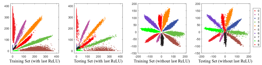
Appendix A The intuition of removing the last ReLU
Standard CNNs usually connect ReLU to the bottom of FC1, so the learned features will only distribute in the non-negative range , which limits the feasible learning space (angle) for the CNNs. To address this shortcoming, both SphereFace and [16] first propose to remove the ReLU nonlinearity that is connected to the bottom of FC1 in SphereFace networks. Intuitively, removing the ReLU can greatly benefit the feature learning, since it provides larger feasible learning space (from angular perspective).
Visualization on MNIST. Fig. 8 shows the 2-D visualization of feature distributions in MNIST with and without the last ReLU. One can observe with ReLU the 2-D feature could only distribute in the first quadrant. Without the last ReLU, the learned feature distribution is much more reasonable.
Appendix B Normalizing the weights could reduce the prior caused by the training data imbalance
We have emphasized in the main paper that normalizing the weights can give better geometric interpretation. Besides this, we also justify why we want to normalize the weights from a different perspective. We find that normalizing the weights can implicitly reduce the prior brought by the training data imbalance issue (e.g., the long-tail distribution of the training data). In other words, we argue that normalizing the weights can partially address the training data imbalance problem.
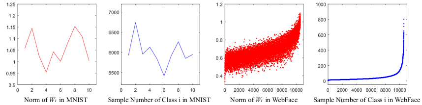
We have an empirical study on the relation between the sample number of each class and the 2-norm of the weights corresponding to the same class (the -th column of is associated to the -th class). By computing the norm of and sample number of class with respect to each class (see Fig. 9), we find that the larger sample number a class has, the larger the associated norm of weights tends to be. We argue that the norm of weights with respect to class is largely determined by its sample distribution and sample number. Therefore, norm of weights can be viewed as a learned prior hidden in training datasets. Eliminating such prior is often beneficial to face verification. This is because face verification requires to test on a dataset whose idenities can not appear in training datasets, so the prior from training dataset should not be transferred to the testing. This prior may even be harmful to face verification performance. To eliminate such prior, we normalize the norm of weights of FC2666FC2 refers to the fully connected layer in the softmax loss (or A-Softmax loss)..
Appendix C Empirical experiment of zeroing out the biases
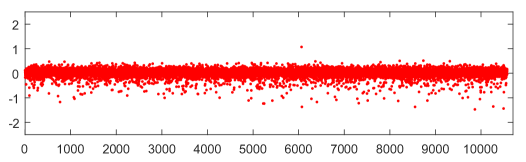
Standard CNNs usually preserve the bias term in the fully connected layers, but these bias terms make it difficult to analyze the proposed A-Softmax loss. This is because SphereFace aims to optimize the angle and produce the angular margin. With bias of FC2, the angular geometry interpretation becomes much more difficult to analyze. To facilitate the analysis, we zero out the bias of FC2 following [16]. By setting the bias of FC2 to zero, the A-Softmax loss has clear geometry interpretation and therefore becomes much easier to analyze. We show all the biases of FC2 from a CASIA-pretrained model in Fig. 10. One can observe that the most of the biases are near zero, indicating these biases are not necessarily useful for face verification.
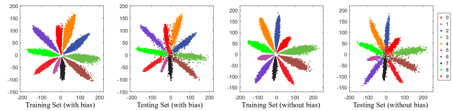
Visualization on MNIST. We visualize the 2-D feature distribution in MNIST dataset with and without bias in Fig. 11. One can observe that zeroing out the bias has no direct influence on the feature distribution. The features learned with and without bias can both make full use of the learning space.
Appendix D 2D visualization of A-Softmax loss on MNIST
We visualize the 2-D feature distribution on MNIST in Fig. 12. It is obvious that with larger the learned features become much more discriminative due to the larger inter-class angular margin. Most importantly, the learned discriminative features also generalize really well in the testing set.
Appendix E Angular Fisher score for evaluating the feature discriminativeness and ablation study on our proposed modifications
We first propose an angular Fisher score for evaluating the feature discriminativeness in angular margin feature learning. The angular Fisher score (AFS) is defined by
| (11) |
where the within-class scatter value is defined as and the between-class scatter value is defined as . is the -th class samples, is the mean vector of features from class , is the mean vector of the whole dataset, and is the sample number of class . In general, the lower the fisher value is, the more discriminative the features are.
Next, we perform a comprehensive ablation study on all the proposed modifications: removing last ReLU, removing Biases, normalizing weights and applying A-Softmax loss. The experiments are performed using the 4-layer CNN described in Table 2. The models are trained on CASIA dataset and tested on LFW dataset. The setting is exactly the same as the LFW experiment in the main paper. As shown in Table 6, we could observe that all our modification leads to peformance improvement and our A-Softmax could greatly increase the angular feature discriminativeness.
| CNN | Remove Last ReLU | Remove Biases | Normalize Weights | A-Softmax | Accuracy | Angular Fisher Score |
|---|---|---|---|---|---|---|
| A | No | No | No | No | 95.13 | 0.3477 |
| B | Yes | No | No | No | 96.37 | 0.2835 |
| C | Yes | Yes | No | No | 96.40 | 0.2815 |
| D | Yes | Yes | Yes | No | 96.63 | 0.2462 |
| E | Yes | Yes | Yes | Yes (m=2) | 97.67 | 0.2277 |
| F | Yes | Yes | Yes | Yes (m=3) | 97.82 | 0.1791 |
| G | Yes | Yes | Yes | Yes (m=4) | 98.20 | 0.1709 |
Appendix F Experiments on MegaFace with different convolutional layers
We also perform the experiment on MegaFace dataset with CNN of different convolutional layers. The results in Table 7 show that the A-Softmax loss could make best use of the network capacity. With more convolutional layers, the A-Softmax loss (i.e., SphereFace) performs better. Most notably, SphereFace with only 4 convolutional layer could peform better than the softmax loss with 64 convolutional layers, which validates the superiority of our A-Softmax loss.
| Method | protocol |
|
|
||||
|---|---|---|---|---|---|---|---|
| Softmax Loss (64 conv layers) | Small | 54.855 | 65.925 | ||||
| SphereFace (4 conv layers) | Small | 57.529 | 68.547 | ||||
| SphereFace (10 conv layers) | Small | 65.335 | 78.069 | ||||
| SphereFace (20 conv layers) | Small | 69.623 | 83.159 | ||||
| SphereFace (36 conv layers) | Small | 71.257 | 84.052 | ||||
| SphereFace (64 conv layers) | Small | 72.729 | 85.561 |
Appendix G The annealing optimization strategy for A-Softmax loss
The optimization of the A-Softmax loss is similar to the L-Softmax loss [16]. We use an annealing optimization strategy to train the network with A-Softmax loss. To be simple, the annealing strategy is essentially supervising the newtork from an easy task (i.e., large ) gradually to a difficult task (i.e., small ). Specifically, we let and start the stochastic gradient descent initially with a very large (it is equivalent to optimizing the original softmax). Then we gradually reduce during training. Ideally can be gradually reduced to zero, but in practice, a small value will usually suffice. In most of our face experiments, decaying to 5 has already lead to impressive results. Smaller could potentially yield a better performance but is also more difficult to train.
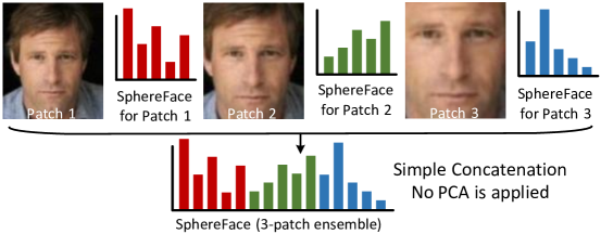
Appendix H Details of the 3-patch ensemble strategy in MegaFace challenge
We adopt a common strategy to perform the 3-patch ensemble, as shown in Fig. 13. Although using more patches could keep increasing the performance, but considering the tradeoff between efficiency and accuracy, we use 3-patch simple concatenation ensemble (without the use of PCA). The 3 patches can be selected by cross-validation. The 3 patches we use in the paper are exactly the same as in Fig. 13.