Beyond the network of plants volatile organic compounds

Abstract

Plants emission of volatile organic compounds (VOCs) is involved in a wide class of ecological functions, as VOCs play a crucial role in plants interactions with biotic and abiotic factors. Accordingly, they vary widely across species and underpin differences in ecological strategy. In this paper, VOCs spontaneously emitted by 109 plant species (belonging to 56 different families) have been qualitatively and quantitatively analysed in order to classify plants species. By using bipartite networks methodology, based on recent advancements in Complex Network Theory, and through the application of complementary classical and advanced community detection algorithms, the possibility to classify species according to chemical classes such as terpenes and sulfur compounds is suggested. This indicates complex network analysis as an advantageous methodology to uncover plants relationships also related to the way they react to the environment where they evolve and adapt.

Introduction

Plants produce an amazing variety of metabolites. Only a few of these are involved in “primary” metabolic pathways, thus common to all organisms; the rest, termed “secondary” metabolites, are characteristic of different plants groups[1]. In fact, “secondary” metabolites, despite the name initially addressed to underline their inessiantiality for primary plant processes[2], are the result of different plants responses, through the course of evolution, to specific needs. Among such metabolites, volatile organic compounds (VOCs) play a dominant role[3]. Being released by quite any kind of tissues[4, 5] and type of vegetation (trees, shrubs, grass, etc.) as green leaf volatiles, nitrogen-containing compounds and aromatic compounds, plants VOCs can be emitted constitutively[6, 7] or in response to a variety of stimuli. They are in fact involved in a wide class of ecological functions, as a consequence of the interactions of plants with biotic and abiotic factors[8]. Plants use VOCs to perform indirect plant defence against insects[9], to attract pollinators[10], for plant-to-plant communication [11, 12], for thermo-tolerance and environmental stress adaptation (see more references in[7]), to defend from predator[13].

According to their biosynthetic origin and chemical structure, plant volatiles can be grouped into isoprenoids or terpenoids, but also oxygenated VOCs (OVOCs), such as methanol (CH₄O), acetone (C₃H₆O), acetaldehyde (C₂H₄O), methyl-ethyl-ketone (MEK, C₄H₈O) and methyl-vinyl-ketone (MVK, C₄H₆O)[14]; in few cases, sulfur compounds (e.g. in Brassicales) and furanocoumarins and their derivatives (e.g in Apiales, Asterales, Fabales, Rosales) are found[15, 16].

Interestingly, VOCs emissions strongly depend on the species (see [17] for references). Indeed, different plant lineages often adopt different chemical solutions to face the same problem; this is the case, for example, of the different odorous volatiles emitted by different flowers for solving the common problem of attracting the same type of pollinator, which usually visit a large amount of plant species[2].

In this paper we apply both complex networks analysis[18, 19, 20] and community detection[21, 22] to identify an eventual hierarchy among the available species, on the basis of their similarities in terms of VOCs emissions. Complex Network Theory[23, 24, 25] has been already successfully used in ecology to determine, for example, the stability and robustness of food webs[26] with respect to the removal of one or more individuals from the network, or in biology to study the structure of protein interactions in the cell by the so-called protein interaction networks (PINs)[27]. Moreover metabolic networks are used to study the biochemical reactions which take place into living cells[28]. Still, biological networks found important applications in medicine[29], where they are applied as a solution to human diseases comorbidity analysis[30], or to study the structural and functional aspects of human brain, by defining the reciprocal interactions of the cerebral areas[31]. Nevertheless, the application of Complex Networks Theory in botany is still scarce, exception made for some tentatives of comparing different ecosystems looking for steady (i.e. “universal”) behaviours[32]. Recent applications of graph theory in botany deal with the attempt of assessing plants species similarities on the basis of both their diaspore morphological properties, and fruit-typology ecological traits[33]. Following the same approach, in this paper we perform network analysis with the goal of identifying communities of “similar” species, starting from the volatiles they emit, or more generally from the ways the species share between them to react to external wounding stimuli.

At this purpose, data are represented by means of bipartite graphs, which are particularly suitable to study the relations between two different classes of objects and to group individuals according to the properties they share. More in details, the vertices of a bipartite graph can be subdivided into two disjoint sets, such that every vertex of one set is connected only with a vertex of the other set. No links are present between vertices belonging to the same set. In our case, the plants species and the volatiles they emit will define the two independent sets of vertices of the bipartite graph built from botanical data. In practice two different graphs can be analysed: the first one is made up by all plants species (as vertices) connected on the basis of the common properties they share, i.e. in that case the amount of VOCs emitted; the second one is made up by VOCs connected accordingly to the plants that share the same emissions. Once the graph are suitably deduced from the experimental data, community detection is a powerful method to classify in a quantitative way the different species creating a taxonomic tree[22].

The paper is organized as it follows: in Section “Results” we present the main outputs of the analysis conducted on the dataset considered; in Section “Discussion” we debate the main implications of our results and we propose possible further developments of the actual study. We refer the reader interested in more details about both data and methodology to Section “Materials and Methods”.

Results and Discussion

The present research work focuses on a group of $75$ volatiles emitted by $109$ different plant species in basal conditions, in order to understand if taxonomy-related plants emit a similar VOC composition. To assure the analysis to be robust and consistent, we measured the volatiles emitted by each plant species by a three times replication experiment. We refer to the section “Materials and methods” for a suitable description of the dataset preparation.

Complex networks analysis is applied to the VOCs dataset represented as bipartite network, in order to easily define metrics and hidden statistical properties able to discriminate and classify plant taxonomy based on VOCs patterns.

Data preprocessing

The $109$ plants species analysed are representative of $56$ families, and the dataset is quite homogeneous in terms of families percentages. The most copious families are: Asteraceae ($8.26\%$), Solanaceae ($6.42\%$), Rosaceae ($6.42\%$), Fabaceae ($5.5\%$), Brassicaceae ($4.59\%$), and Polygonaceae ($3.67\%$). All the other families are present at lower percentages.

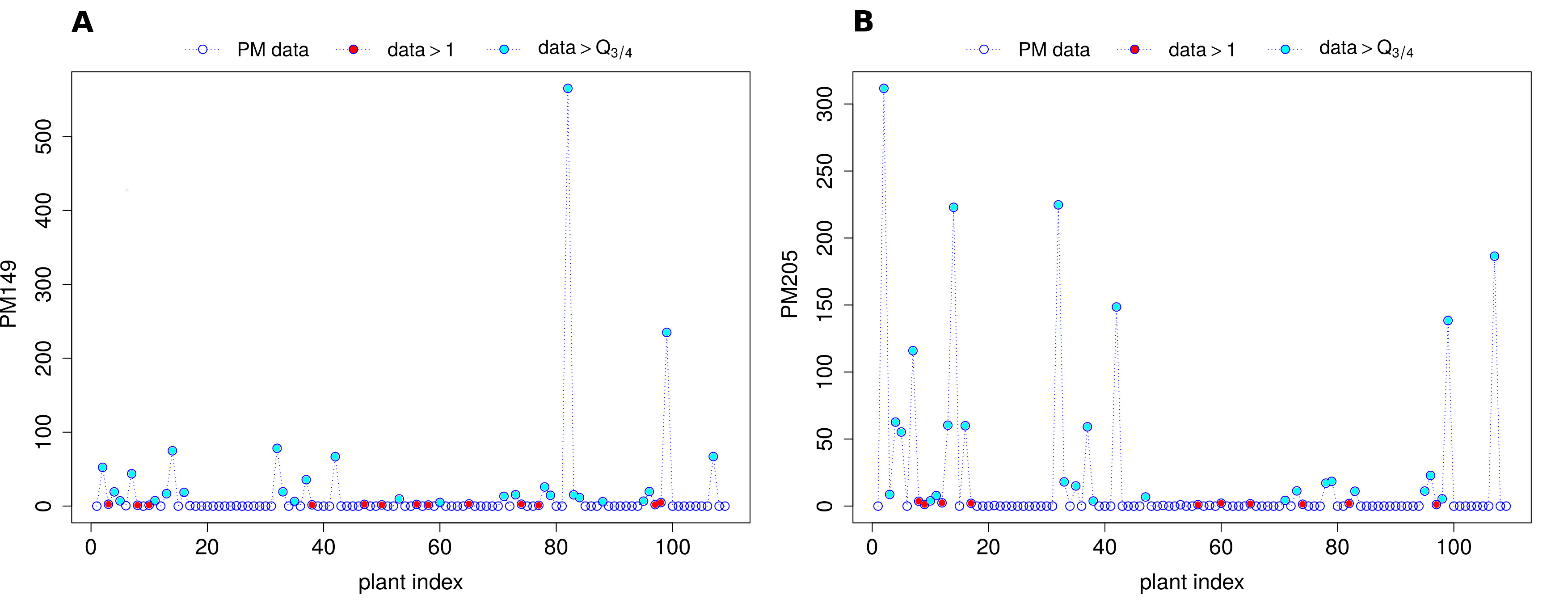
Figure 1: PM$149$ (Tp/STp-f) (panel A) and PM$205$ (STp) (panel B) emissions. Protonated mass data are represented by empty blue bullets. Red dots correspond to values larger than 1, while cyan dots refer to those data exceeding $Q_{\frac{3}{4}}$. x-axis: plants index. Protonated masses are expressed as mass-to-charge (m/z) ratios.

To evaluate the data statistical structure we plotted for each protonated mass the emission recorded for all the $109$ plants species. Figure 1 (empty blue bullets) shows the emission of protonated masses PM$149$ (panel A) and PM$205$ (panel B), as two examples of VOCs records behaviour. Protonated masses are expressed as mass-to-charge (m/z) ratios. From the chemical composition point of view, PM$149$ and PM$205$ belong to terpenes/sesquiterpenes fragments (Tp/STp-f) and sesquiterpenes (STp) classes, respectively. The VOCs series turn out to be characterized by the superposition of an irregular, abruptly changing pulsatile component and a slowly changing one. More in details, zero-values indicate the lack of emission of that specific VOC for the corresponding plants, and the flat and uniform plateau suggests a small emission of the same VOC. Finally, spike-like pulses, clearly emerging from the background, are related to a huge emission of that VOC for a given plant. Figure 1 suggests that both the protonated masses PM$149$ and PM$205$ are emitted in large quantity just by few species. That behaviour turned out to be representative of the whole dataset (not shown).

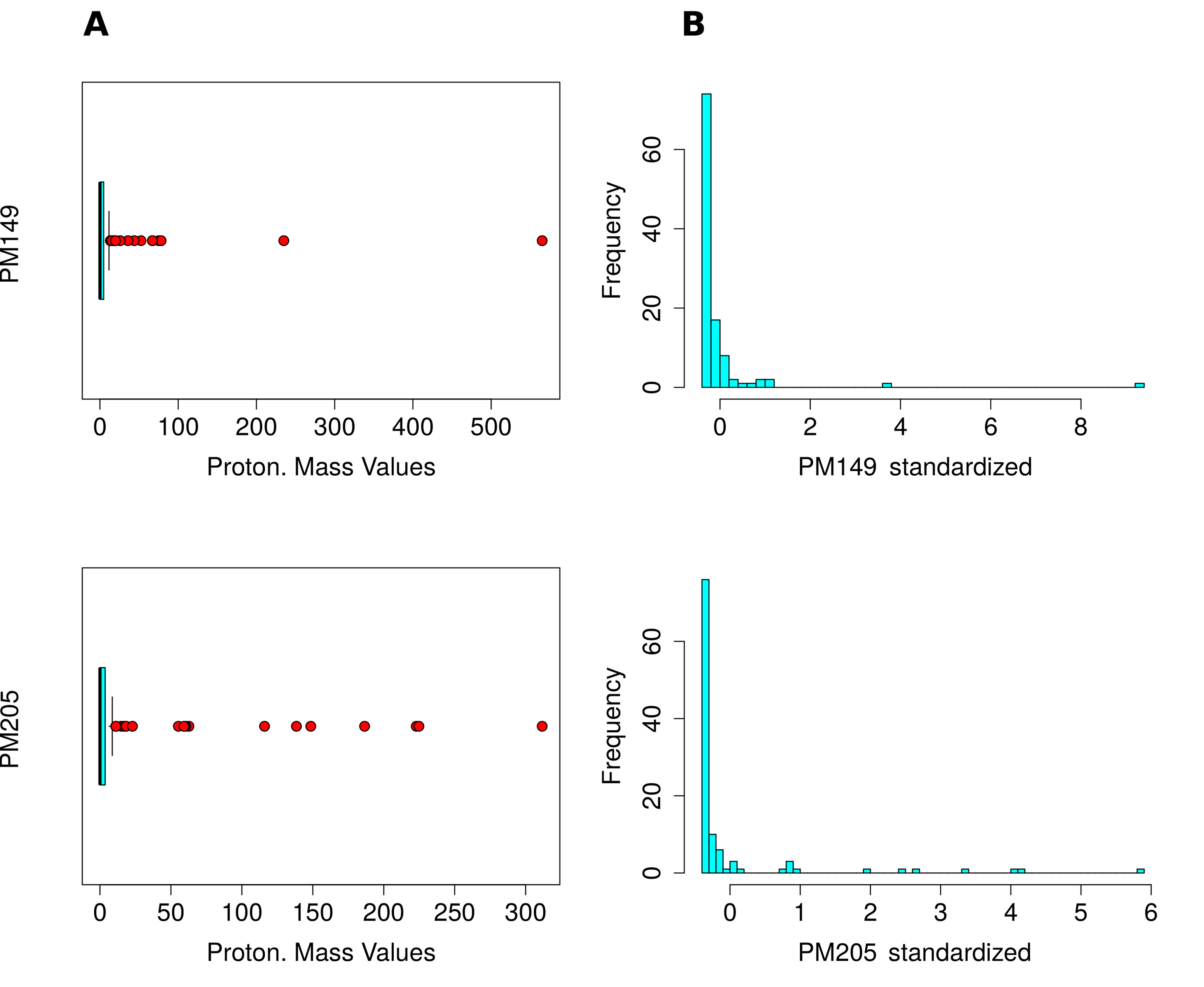
Figure 2: PM$149$ (Tp/STp-f) and PM$205$ (STp) emissions. Panels A: boxplots, $IQR$ (cyan rectangles) and outliers (red dots). Panels B: Absolute frequency histograms (y-axes) versus data standardized values (x-axes), obtained by removing the sample mean, and by normalizing the residuals to the sample standard deviation. Protonated masses are expressed as mass-to-charge (m/z) ratios.

From a statistical point of view the same result was confirmed by the presence of outliers inside each record, that can be easily visualized by boxplot methodology[34, 35] (see Section “Materials and methods” for more details). Outliers are shown in Fig. 2 (panels A, red dots), and they correspond to those observations far from the sample mean. In that case, since the behaviour was coherent for all the VOCs, we excluded the presence of outliers as a consequence of merely experimental errors. Rather, protonated mass records were characterized by heavy-tailed distribution, as Fig. 2 (panels B) shows: few values lie in the queues of the absolute frequencies sample data histograms. Standardized values were employed in order to assure the results comparability.

Notwithstanding the clear dominating behaviour of some species emissions with respect to the other plants, for a given VOC, the statistical procedure of taking into account just the highest recorded values (extreme values) turned out to be too restrictive. In fact, not even a small emission of a protonated mass can be neglected from an experimental point of view. A low emission is as well a signal from a wounded leaf, and it has to be taken carefully into account when comparing the several species reciprocal behaviour with respect to an external wounding perturbation.

Basic network analysis

We considered two different ways of building the plants network, depending on the statistical measure used to represent the highly not-gaussian behaviour of the series. In the first case, we set a fixed threshold for the signal intensity ($1$ normalized counts per second, ncps) and we considered significant all the emissions larger than it (graph: $G_{1}(V,E)$). In the second case, we applied a more severe criterion, and we decided to take into account just the emissions above the third quartile of the corresponding data statistical distribution, i.e. $Q_{\frac{3}{4}}$ (graph: $G_{2}(V,E)$). Figure 1 shows both the approaches applied to PM$149.1$ (panel A) and PM$205.1$ (panel B). Red dots in both panels highlight values larger than $1$, while cyan bullets represent the value exceeding $Q_{\frac{3}{4}}$.

In both cases, a bipartite network was build, made up by $V=184$ vertices, subdivided into two layers: the first one made up by $V_{P}=109$ plants species and the second one composed by $V_{PM}=75$ emitted VOCs. By definition of bipartite graph, connections were possible between vertices belonging to the two different layers, only. No links are present among plants, as well as among VOCs. Plants species networks are subsequently defined by considering as vertices the plant species in the database, so as bipartite projections of both $G_{1}(V,E)$ and $G_{2}(V,E)$. Two vertices are connected if they share at least one common property, in other words, if they emit almost the same amount of a specific VOC. For every network, we considered size (number of edges), order (number of vertices), degree (average and its distribution), density (the ratio of actual vertices against the possible ones), clustering and finally the community structure.

Threshold-based graph

The plants graph corresponding to the first method was created as a bipartite projection of graph $G_{1}(V,E)$. In the resulting graph $G^{P}_{1}(V_{1},E_{1})$ plants are interconnected on the basis of the common VOCs they emit. $G^{P}_{1}(V_{1},E_{1})$ is made up of $V_{1}=V_{P}=109$ vertices (plant species), and $E_{1}=5,886$ edges. Species $i$ and species $j$ are linked if they share at least one common emitted protonated mass. The weight $w_{ij}$ of each link $e_{ij}$ is given by the total number of shared VOCs between species $i$ and species $j$. $G^{P}_{1}(V_{1},E_{1})$ is a fully connected graph, its density $D=\frac{2E_{1}}{V_{1}(V_{1}-1)}$ is equal to 1, and the degree of each node is equal to $108$, which is also equal to the nodes mean degree ($\overline{k}=\frac{1}{V_{1}}\sum_{i=1}^{V_{1}}k_{i}=\frac{2E_{1}}{V_{1}}$). Each vertex is connected to all the other vertices, or equivalently each species emits at least one VOCs in common with all the other species.

That network structure is poorly able to extract information about the dominant behaviour of one species with respect to the others, in terms of their emissions. Concerning the links weights distribution, the maximum number of protonated masses shared by two species is $66$, and in average species are connected by links of weight $w_{ij}=24$, in agreement with the dense structure of the network.

Third-quartile-based graph

The plants graph corresponding to the second test was analogously constructed as the species-vs-species bipartite projection graph of $G_{2}(V,E)$ graph. Again, the common emitted VOCs determine the presence or not of a (weighted) link between two nodes. $G^{P}_{2}(V_{2},E_{2})$ is made up by $V_{2}=V_{P}=109$ vertices and $E_{2}=2,343$ edges. Links are less by construction: in that case, for each VOC just the emissions larger than $Q_{\frac{3}{4}}$ were considered significant. It follows that the network construction procedure accounted for a more severe pruning. Graph density reduces to 0.39 consistent with the fact that the graph is not fully connected. Rather, isolated vertices emerge, suggesting the presence of plants which do not emit any of the measured VOCs at a high level. By removing them the graph density increase to $0.73$.

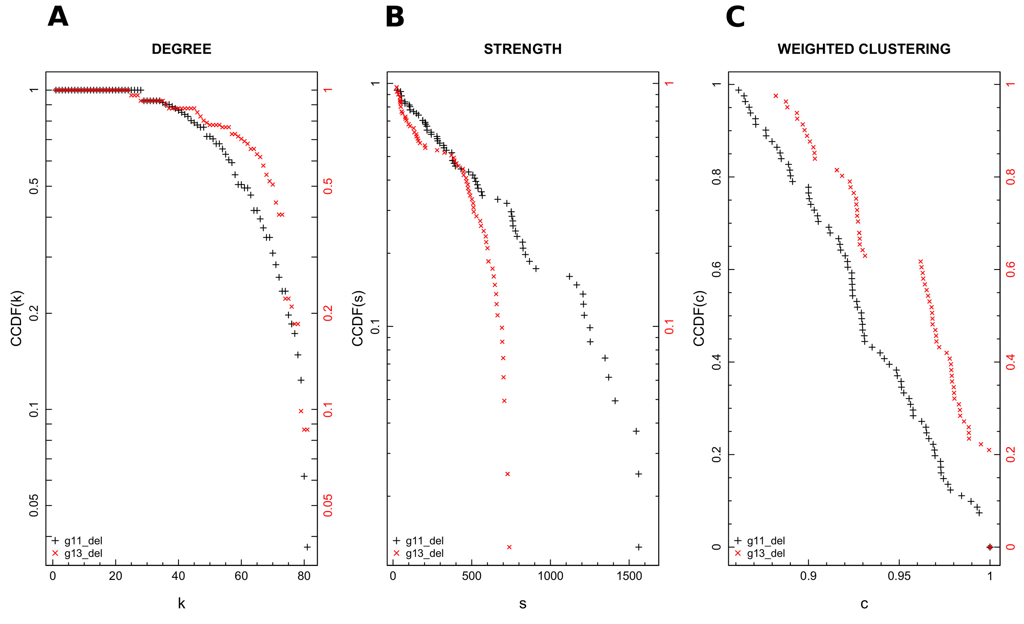
Figure 3: Complementary cumulative distribution functions (CCDF) of degree and strength are reported in log-line scale in panel A and B, respectively, for both $G^{P}_{2}(V_{2},E_{2})$ (black crosses) and $G^{P}_{3}(V_{3},E_{3})$ (red crosses). Panel C, moreover, shows weighted clustering coefficient distribution. More precisely, CCDF (on y-axis) is plotted versus the weighted clustering parameter (x-axis) on linear scale. The isolated nodes were not taken into account for the corresponding network’s basic metric analysis.

In that case the majority of species share few common VOCs emitted (i.e. the mean of the edges weights is around $5$). On the contrary some vertices are connected by heavy links (the maximum weight’s value is $67$, similarly to the previous case). Figure 3 (panel A, black crosses) shows the network degree distribution $P(k)$, representing the fraction of vertices with degree $K>k$. A log-line plot is chosen to display the degree complementary cumulative distribution function (CCDF). The graph strength distribution is also shown in Fig. 3 (panel B, black crosses) in log-line scale. The strength $s$ of a vertex corresponds practically to its weighted degree, thus it takes into account the total weight of the vertex connections, and it allows one to identify high and low concentration edges-regions inside an undirected graph. The maximum strength value is equal to $s_{max}=1,624$ and it corresponds to Lavandula spica L. (Lavender) species, the minimum is equal to $s_{min}=27$ and it is common to Humulus lupulus L. (Wild hop), Actinidia arguta (Siebold & Zucc.) (Hardy kiwi), Ficus benjamina L. (Weeping fig), Magnolia liliiflora (Desr.) (Japanese magnolia), and Diospyros lotus L. (Date-plum) species. Finally, Fig. 3 (panel C) shows the local clustering coefficient, defined as the tendency among two vertices to be connected if they share a mutual neighbour.

Taken as a whole, Fig. 3 suggests that plants network is not dominated by some central nodes with a huge amount of connections linking them to all the other minor vertices. Notwithstanding, some species emit a large quantity of VOCs and communities detection algorithms are applied to identify them and the respective aggregating VOCs. The graph $G^{P}_{2}(V_{2},E_{2})$ isolated nodes were removed before performing that basic metrics analysis for visual reasons. The degree and strength of an isolated node are equal to $0$ by definition and the clustering coefficient is not defined.

Selected-VOCs graph

A third test was performed on a reduced version of the original database. Certain VOCs which could be more strictly associated to the mechanical wounding performed during the sample measurements than to plant species-specific emissions were excluded. Indeed, certain compounds such as methanol, acethaldeyde, some C6-compounds, etc. [36, 37] are produced by almost all plant species, but there is no a common behaviour in terms of quality and quantity of VOCs involved [38, 39]; their inclusion in the database could lead to misinterpretation. Furthermore, other compounds that turned out to be less powerful in the aggregation features, as highlighted by the above described analyses, were removed from the dataset. As a result, a selection of $30$ protonated masses were taken into account.

In order to compensate that filter introduced by the hand-made choice of the relevant VOCs to be considered for the analysis, a threshold equal to $0$ was used to distinguish between relevant and negligible emissions of that specific VOC. The corresponding bipartite network $G_{3}(V,E)$ was made up by $V=139$ vertices subdivided in two sets: $V_{P}=109$, analogously to previous graphs, and $V_{PM}=30$. In order to study plants network, the bipartite projection $G^{P}_{3}(V_{3},E_{3})$ was analysed. The vertices are still $V_{3}=V_{P}=109$, while the edges are equal to $E_{3}=2,522$, similarly to the third-quartile-based graph. The graph density is $0.43$ due to the presence of $28$ isolated nodes, while it raises to $0.78$ if they are removed. Concerning the graph basic metrics, Fig. 3 (panel A, red crosses) shows $G^{P}_{3}(V_{3},E_{3})$ complementary cumulative degree distribution $P(k)$, while Fig. 3 (panel C, red crosses) depicts the graph strength distribution. Both figures are in log-line scale. The network strength maximum value decreases to $s_{max}=746$, but it still corresponds to Lavandula spica L. (Lavender) species, which again emerges as the most connected node. On the other side, the strength minimum value is $s_{min}=23$ for Cyperus papyrus L. (Papyrus), Salicornia europaea L. (Glasswort), and Solanum quitoense Lam. (Naranjilla) species. Further, $G^{P}_{3}(V_{3},E_{3})$ is characterized by a smaller range of strength values with respect to $G^{P}_{2}(V_{2},E_{2})$, and a more restricted set of nodes seem to dominate the network behaviour. Nevertheless, the graph degree and strength distribution do not suggest the presence of a scale-free structure behind our data. Finally, Fig. 3 (panel C, red crosses) shows $G^{P}_{3}(V_{3},E_{3})$ clustering coefficient. The behaviour is similar to the one observed for $G^{P}_{2}(V_{2},E_{2})$ graph. Such as for $G^{P}_{2}(V_{2},E_{2})$ graph, isolated nodes were removed before performing that basic metrics analysis. Analogously, the strength minimum value is performed after excluding the isolate nodes, since the degree $k$ and thus the strength $s$ of an isolated node are equal to $0$ by definition.

Community detection analysis

Threshold-based and third-quartile-based graphs

A first attempt to group plants on the basis of the VOCs emitted was performed by applying the community detection to both the dense $G^{P}_{1}(V_{1},E_{1})$ graph and the third-quartile-based graph $G^{P}_{2}(V_{2},E_{2})$. For both of them, subgraphs were obtained filtering-out a growing number of links, from the lower to the higher weighted ones. A unit-based normalization was applied to edges weights to limit their values to the [0, 1] range ($w^{resc}_{ij}$ parameter in Tab 1). Four communities detection algorithms were applied: (i) Louvain or Blondel’s modularity optimization algorithm (BL), (ii) fast greedy hierarchical agglomeration algorithm (FG), (iii) walktrap community finding algorithm (WT), and (vi) label propagation community detection method (LP). We refer to the section “Materials and methods” for a detailed description of the communities detection methods.

FG	WT	BL	LP	$w^{resc}_{ij}$	E	N	is.connected	density
2	2	2	1	0	5886	109	TRUE	1
2	2	2	1	0.1	5303	104	TRUE	0.99
2	2	2	1	0.2	4776	101	TRUE	0.95
2	2	2	1	0.3	3220	85	TRUE	0.9
2	2	2	1	0.4	1316	58	TRUE	0.8
2	1	3	1	0.5	697	44	TRUE	0.74
2	28	2	1	0.6	309	28	TRUE	0.81
2	4	2	1	0.7	156	21	TRUE	0.74
2	12	2	1	0.8	48	12	TRUE	0.73
2	3	2	1	0.9	13	7	TRUE	0.62
1	2	1	1	1	1	2	TRUE	1

Table 1: Communities detection of graph $G^{P}_{1}(V_{1},E_{1})$ by fast greedy (FG), walktrap algorithms (WT), Blondel modularity optimization (BL), and label propagation (LB). Several filtered-by-edges-weight versions of the graph were analysed (one for each row). Graph edges weight values are normalized to the interval $\left[0,1\right]$.

Notwithstanding some discrepancies in the results depending on algorithms optimization after pruning the network, two big communities emerge from $G^{P}_{1}(V_{1},E_{1})$ analysis, which turned out to be robust to algorithm changes and to the filtering procedure of the edges weights (see Tab. 1), exception made for severe filters (rescaled weight parameter $w_{ij}>0.5$ in Tab. 1). In that case, almost half of the graph nodes were filtered out, thus reducing the reliability of the related results as the consequence of a huge loss of information. On the contrary, by pruning the graph from the most heavy links, the results were statistically comparable thus meaning that the plants network was not dominated by some big vertices acting as hubs of the whole system. The two uncover communities embed the $61.47\%$ and $38.53\%$ of the total amount of species inside the database, respectively.

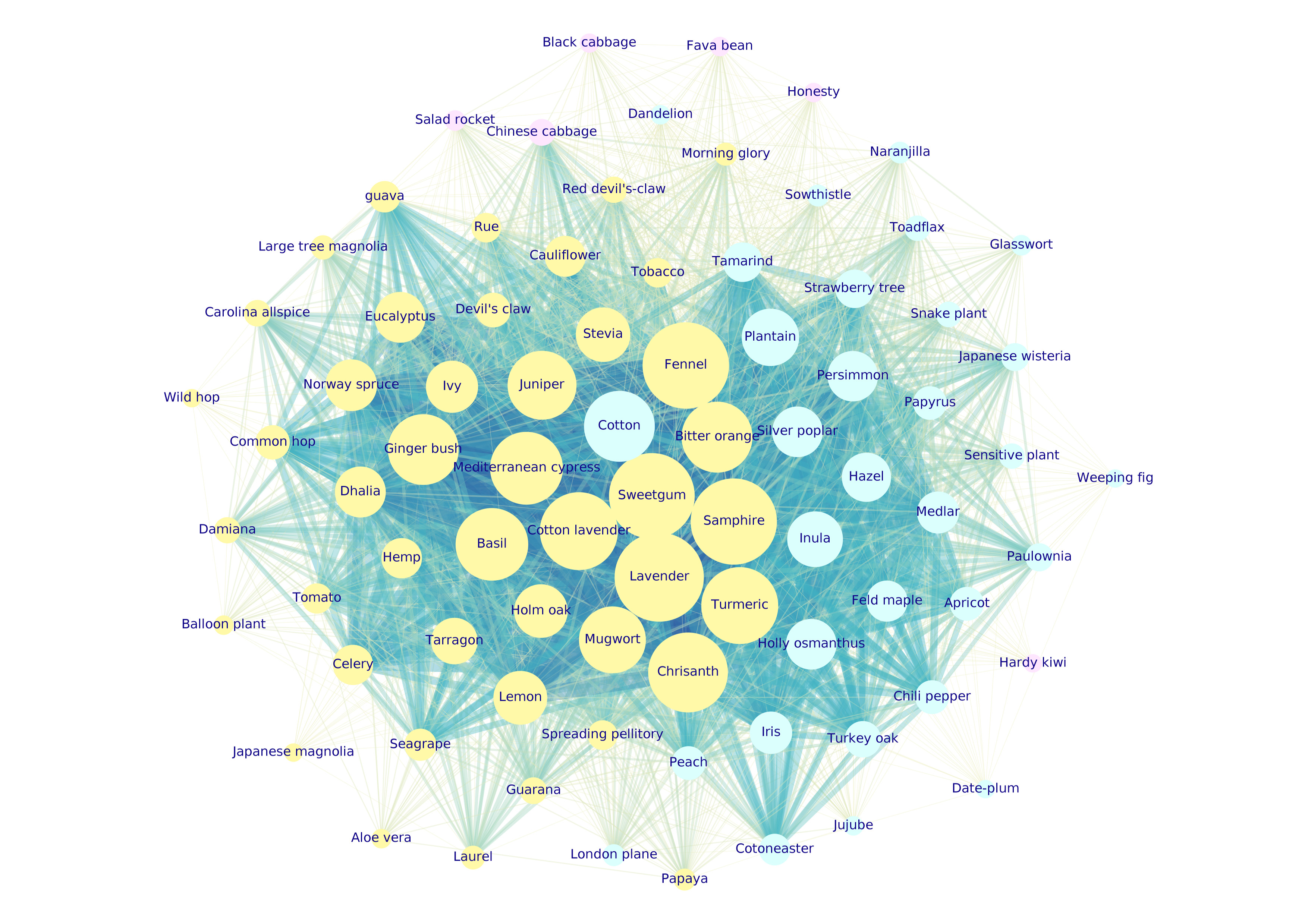
Figure 4: $G^{P}_{2}(V_{2},E_{2})$ third-quartile-based graph. Each color corresponds to one detected community: cluster $1$ (yellow), cluster $2$ (aqua), cluster $3$ (violet). The $28$ isolated nodes are not shown (cluster $4$). Nodes dimension is proportional to nodes weighted degree. Edges thickness is proportional to the edges weight. Lavandula spica L. (Lavander), Foeniculum vulgare Mill. (Fennel), Crithmum maritimum L. (Samphire), Liquidambar styraciflua L. (Sweetgum), visible as biggest yellow nodes, are some of the most active species in terms of VOCs emissions.

The situation improved by analyzing the communities of $G^{P}_{2}(V_{2},E_{2})$ graph. Figure 4 is a representation of $G^{P}_{2}(V_{2},E_{2})$ plants network. The dimension of each node is proportional to the node’s weighted degree. The thickness of each link connecting two nodes $i$ and $j$ is proportional to the link’s weight, $w_{ij}$. Nodes colours refer to cluster membership. In that case two big clusters emerge from a basic community detection. They embed $44$ and $31$ species, i.e. respectively the $40.4\%$ and $28.4\%$ of the species present in the dataset (yellow and aqua clusters in Fig. 4). Brassicaceae family started to be pretty grouped in a third small family ($6$ species only accounting for the $5.5\%$ of the species dataset, violet cluster of Fig. 4), exception made for the Brassica oleracea L. var botrytis species (Cauliflower) which belongs to another community (yellow cluster in Fig.4). By construction $28$ isolated nodes emerged (not shown in Fig. 4), corresponding to species which were not sharing any of the measured VOCs with the other plants. Isolated nodes accounted for the $25.7\%$ of species total amount. Again, the results were consequent to the simultaneous application of more than a single methodology. The findings proved to be independent from the applied methodology and they were considered robust and reliable from a statistical point of view. Hereafter, the composition of every cluster is summarised, together with the protonated mass that the species share at graph’s communities level:

• cluster $1$: $31$ species ($28.4\%$ of the database total species) grouped in $21$ families; prevailing families: Rosaceae, Asteraceae, Fabaceae, Ebenaceae, Plantaginaceae, and Solanaceae. Two VOCs in particular are responsible for that partitioning: PM$27$ (hydrocarbons, Hyd) and PM$73$ (acids, A) ($20$ species), followed by PM$55$ (aldehydes fragment, Ald-f), PM$89$ (esters, E), PM$115$ (acids, A) ($19$ species), and PM$53$ (fragment, f), PM$81$ (aldehydes fragments, Ald-f) ($18$ species). In general, the more informative VOCs for this cluster are compounds belonging to several chemical classes. Notice that from $m/z=123$ (PM$123$) to $m/z=205$ (PM$205$), where peaks deriving from terpenes, sesquiterpenes and their fragments are found, the emissions are null for all the species. One species can emit more than one VOC, so that all the species can be counted more than once to assess how many species share the same protonated mass emission. Gossypium herbaceum L. (Cotton), Plantago lanceolata L. (Plantain), and Inula viscosa L. (Inula) species are between the highest weighted degree nodes in Fig. 4.

• cluster $2$: it is the biggest community, made up of $44$ species ($40.4\%$ of the total species amount) grouped into $27$ families; dominant families: Asteraceae, Apiaceae, Cannabaceae, Lamiaceae. The species belonging to that cluster emit, taken as a whole, a large amount of VOCs. They share in particular the emission of VOCs which are or refer to terpenes compounds, which are among the principal odour-like molecules emitted by plants flowers and leaves. In details, 28 species share PM$123$ and PM$135$, both terpenes or sesquiterpenes fragments (Tp/STp-f); 27 species share PM$93$ (Tp-f), PM$95$ (STp-f), PM$105$ (heterocyclic aromatic compounds, HeArC), PM$109$ (Tp-f), PM$119$ (Tp-f), PM$121$ (Tp-f), PM$137$ (Tp/STp-f), PM$143$ (ketones and aldehydes, K/Ald), PM$149$ (Tp/STp-f), PM$163$ (STp-f), PM$205$ (STp); $26$ species share PM$91$ (hydrocarbons, Hyd), PM$107$ (HeArC), PM$111$ (aldehydes, Ald), PM$153$ (Tp-f).

  Accordingly, that community includes plant species characterized by intense flavour, such as Lavandula spica L. (Lavander, a well known plant used for its flavour), Foeniculum vulgare Mill. (Fennel, an anise-flavored spice), Crithmum maritimum L. (Samphire, a very flavoured sea fennel), and Liquidambar styraciflua L. (Sweetgum, commonly used as flavor and fragrance agent). A more detailed description of cluster $2$ is supplied hereafter.

• cluster $3$: $6$ species only ($5.5\%$ of total species) from $3$ families: Brassicaceae (dominating family with $4$ species), Actinidiaceae, and Fabaceae. Interestingly, the Brassicaceae Cauliflower belongs to the previous community (i.e., to cluster $2$, where species characterized by more intense odours and presence of terpenes compounds are clustered). Indeed, Cauliflower is, among the Brassicacaeae species included in the present study, one of the richest in VOCs and terpenes [40, 41]. This is the most homogeneous community in terms of family composition. PM$63$, a typical sulfur compound (SC), is the most emitted VOC, being released by $5$ species ($4$ of them belonging to the Brassicaceae family), followed by another sulfur compound, PM$49$, and PM$83$ (alcohols fragment, Alc-f) ($3$ species), PM$87$ (Ald/Alc). In particular Brassica rapa L. (Chinese cabbage) emits also PM$85$ (Alc-f), PM$103$ (esters, E), PM$117$ (Alc), PM$129$ (Alc), PM$143$ (ketones and aldehydes, K/Ald). The latter protonated mass, tentatively identified as 2-Nonanone [42] has been already reported in Chinese cabbage[43]. The emission of all the other VOCs is null for the whole species set.

• cluster $4$: $28$ isolated species ($25.7\%$ of total species) belonging to $20$ different families dominated by Polygonaceae, Rosaceae, Solanaceae, Araceae, Fabaceae. They do not share any emitted VOC with other plants, since they do not release any protonated mass at all. That result has to be interpreted taking into account $G^{P}_{2}(V_{2},E_{2})$ construction procedure. Just the emissions exceeding the $Q_{\frac{3}{4}}$ of the corresponding protonated mass distribution were considered as relevant. In that sense that nodes are isolated from the rest of the graph and they do not emit VOCs.

Previous results are summarized in Tab. 2, which shows the dominant families in each cluster and how many species belong to that families. The list of species present in each cluster is reported in Tab. 3.

Cluster $2$, besides being the biggest one, is made up by those species corresponding to the highest weighted degree vertices in $G^{P}_{2}(V_{2},E_{2})$. That species work as highly connected nodes, and they share several VOCs with the other neighboring nodes. They correspond to the biggest yellow nodes in Fig. 4. Here we list the principal ones: Lavandula spica L. (Lavander), Foeniculum vulgare Mill. (Fennel), Crithmum maritimum L. (Samphire), Liquidambar styraciflua L. (Sweetgum), Chrysanthemum indicum L. (Chrisanth), Santolina chamaecyparissus L. (Cotton lavender), Curcuma longa L. (Turmeric), Cupressus sempervirens L. (Mediterranean cypress), Ocimum basilicum L. (Basil), Citrus x Aurantium L. (Bitter orange), Tetradenia riparia (Hochst.) Codd. (Ginger bush), Juniperus communis L. (Juniper), Artemisia vulgaris L. (Mugwort), Citrus x Limon L. (Lemon), Stevia rebaudiana (Stevia), Eucalyptus globulus L. (Eucalyptus), Quercus ilex L. (Holm oak), Hedera helix L. (Ivy).

Other species with as well a huge emission of VOCs are present in cluster $1$: Gossypium herbaceum L. (Cotton), Plantago lanceolata L. (Plantain), and Inula viscosa L. (Inula) are the most connected aqua nodes in Fig. 4.

Cluster $3$ (violet vertices in Fig. 4.) turns out to be the most homogeneous one in terms of families composition, since it groups species belonging mainly to $Brassicaceae$ family, characterized by the predominant emission of sulphur compounds.

cluster $1$		cluster $2$		cluster $3$		cluster $4$
Rosaceae	4	Asteraceae	5	Brassicaceae	4	Polygonaceae	3
Asteraceae	3	Apiaceae	3	Actinidiaceae	1	Rosaceae	3
Fabaceae	3	Cannabaceae	3	Fabaceae	1	Solanaceae	3
Ebenaceae	2	Lamiaceae	3			Araceae	2
Plantaginaceae	2	Cupressaceae	2			Fabaceae	2
Solanaceae	2	Magnoliaceae	2			Apocynaceae	1
Amaranthaceae	1	Martyniaceae	2			Aquifoliaceae	1
Asparagaceae	1	Myrtaceae	2			Asteraceae	1
Betulaceae	1	Rutaceae	2			Crassulaceae	1
Cyperaceae	1	Sapindaceae	2			Faboideae	1
Ericaceae	1	Solanaceae	2			Hydrangeaceae	1
Fagaceae	1	Araliaceae	1			Iridaceae	1
Iridoideae	1	Brassicaceae	1			Lauraceae	1
Malvaceae	1	Calycanthaceae	1			Lythraceae	1
Moraceae	1	Caricaceae	1			Malvaceae	1
Oleaceae	1	Composite	1			Moraceae	1
Paulowniaceae	1	Convolvulaceae	1			Oleaceae	1
Platanaceae	1	Fagaceae	1			Poaceae	1
Rhamnaceae	1	Hamamelidaceae	1			Portulacaceae	1
Salicaceae	1	Lauraceae	1			Vitaceae	1
Sapindaceae	1	Pinaceae	1
		Polygonaceae	1
		Rutacee	1
		Turneraceae	1
		Urticaceae	1
		Xanthorrhoeaceae	1
		Zingiberaceae	1
Fam.	$\#$ Spec.	Fam.	$\#$ Spec.	Fam.	$\#$ Spec.	Fam.	$\#$ Spec.

Table 2: Plants families composition in each community extracted from third-quartile-based graph $G^{P}_{2}(V_{2},E_{2})$ by modularity (BL) algorithm, and the corresponding amount of species belonging to that families for each community. Exception made for cluster $3$ (violet), a huge families heterogeneity characterizes all the other communities.

cluster $1$		cluster $2$		cluster $3$		cluster $4$
Mimosa pudica L.	Fabaceae	Ocimum basilicum L.	Lamiaceae	Brassica rapa L.	Brassicaceae	Zamioculcas zamiifolia (Lodd.)	Araceae
Cyperus papyrus L.	Cyperaceae	Brassica oleracea L. var botrytis	Brassicaceae	Brassica oleracea L. var acephala	Brassicaceae	Rheum rhabarbarum L.	Polygonaceae
Ziziphus jujuba Mill.	Rhamnaceae	Stevia rebaudiana	Asteraceae	Actinidia arguta (Siebold & Zucc.)	Actinidiaceae	Hydrangea macrophylla (Lam.)	Hydrangeaceae
Platanus x Acerifolia (Willd.)	Platanaceae	Cannabis sativa L.	Cannabaceae	Eruca sativa (Mill.)	Brassicaceae	Solanum marginatum L.	Solanaceae
Plantago lanceolata L.	Plantaginaceae	Nicotiana tabacum L.	Solanaceae	Vicia faba L.	Fabaceae	Persea americana Mill.	Lauraceae
Arbutus unedo L.	Ericaceae	Eucalyptus globulus L.	Myrtaceae	Lunaria annua L.	Brassicaceae	Vitis vinifera L.	Vitaceae
Cotoneaster horizontalis Decne.	Rosaceae	Ibicella lutea L.	Martyniaceae			Echeveria elegans (Rose)	Crassulaceae
Sonchus oleraceus L.	Asteraceae	Proboscidea parviflora (Woot. & Standl.)	Martyniaceae			Arundo donax L.	Poaceae
Inula viscosa L.	Asteraceae	Quercus ilex L.	Fagaceae			Rumex acetosella L.	Polygonaceae
Corylus avellana L.	Betulaceae	Artemisia dracunculus L.	Composite			Acacia dealbata Link	Fabaceae
Prunus armeniaca L.	Rosaceae	Convolvulus cneorum L.	Convolvulaceae			Robinia pseudoacacia L.	Faboideae
Acer campestre L.	Sapindaceae	Juniperus communis L.	Cupressaceae			Olea europaea L.	Oleaceae
Osmanthus heterophyllus (G. Don)	Oleaceae	Santolina chamaecyparissus L.	Asteraceae			Fragaria vesca L.	Rosaceae
Diospyros kaki L.	Ebenaceae	Apium graveolens L.	Apiaceae			Rosa chinensis (Jacq.)	Rosaceae
Ficus benjamina L.	Moraceae	Ruta graveolens L.	Rutacee			Trifolium pratense L.	Fabaceae
Populus alba L.	Salicaceae	Parietaria judaica L.	Urticaceae			Anthurium andreanum Lind.	Araceae
Iris germanica L.	Iridoideae	Cupressus sempervirens L.	Cupressaceae			Ficus carica L.	Moraceae
Quercus cerris L.	Fagaceae	Calycanthus floridus L.	Calycanthaceae			Ilex aquifolium L.	Aquifoliaceae
Tamarindus indica L.	Fabaceae	Picea abies L.	Pinaceae			Pyrus communis L.	Rosaceae
Salicornia europaea L.	Amaranthaceae	Humulus lupulus L. var. Cascade	Cannabaceae			Silybum marianum L.	Asteraceae
Solanum quitoense Lam.	Solanaceae	Humulus lupulus L.	Cannabaceae			Portulaca oleracea L.	Portulacaceae
Sansevieria trifasciata Prain.	Asparagaceae	Hedera helix L.	Araliaceae			Capsicum chacoense Hunz.	Solanaceae
Diospyros lotus L.	Ebenaceae	Cardiospermum halicacabum L.	Sapindaceae			Withania somnifera L.	Solanaceae
Linaria vulgaris Mill.	Plantaginaceae	Curcuma longa L.	Zingiberaceae			Rumex acetosa L.	Polygonaceae
Taraxacum officinale F.H. Wigg	Asteraceae	Foeniculum vulgare Mill.	Apiaceae			Punica granatum L.	Lythraceae
Wisteria floribunda (Willd.)	Fabaceae	Laurus nobilis L.	Lauraceae			Nerium oleander L.	Apocynaceae
Gossypium herbaceum L.	Malvaceae	Magnolia grandiflora L.	Magnoliaceae			Iris pallida Lamm.	Iridaceae
Mespilus germanica L.	Rosaceae	Citrus x Aurantium L.	Rutaceae			Hibiscus syriacus L.	Malvaceae
Prunus persica L.	Rosaceae	Carica papaya L.	Caricaceae
Paulownia tomentosa Steud.	Paulowniaceae	Aloe vera L.	Xanthorrhoeaceae
Capsicum annuum L.	Solanaceae	Liquidambar styraciflua L.	Hamamelidaceae
		Artemisia vulgaris L.	Asteraceae
		Magnolia liliiflora (Desr.)	Magnoliaceae
		Solanum lycopersicum L.	Solanaceae
		Chrysanthemum indicum L.	Asteraceae
		Tetradenia riparia (Hochst.) Codd.	Lamiaceae
		Crithmum maritimum L.	Apiaceae
		Paullinia cupana Kunth.	Sapindaceae
		Coccoloba uvifera L.	Polygonaceae
		Turnera afrodisiaca Ward.	Turneraceae
		Citrus Limon L.	Rutaceae
		Psidium guajava L.	Myrtaceae
		Lavandula spica L.	Lamiaceae
		Dahlia pinnata Cav.	Asteraceae
Spec.	Fam.	Spec.	Fam	Spec.	Fam.	Spec.	Fam.

Table 3: Species composition of each cluster found in $G^{P}_{2}(V_{2},E_{2})$ third-quartile-based graph. Cluster $4$ is made up by the isolated nodes, i.e. by all that species which don’t share any VOCs with all the other species.

Selected VOCs graph

Communities detection algorithms were applied to the $G^{P}_{3}(V_{3},E_{3})$ following the same procedure described for $G^{P}_{2}(V_{2},E_{2})$ graph. The VOCs reduction reflected into a more clear picture of species reciprocal behaviour in terms of emitted protonated masses. Besides the set of $28$ isolated nodes, tree big communities were detected.

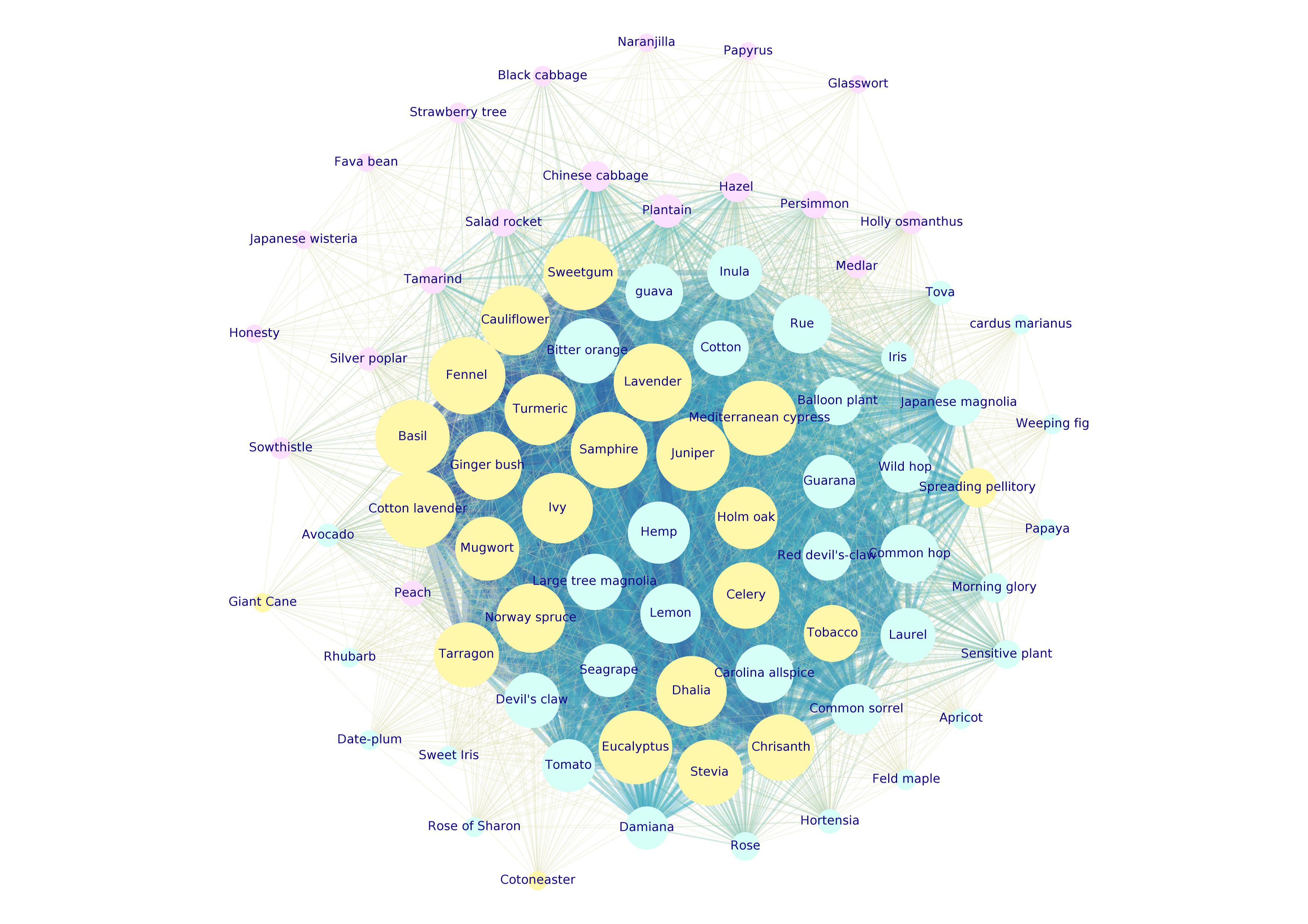
Figure 5: $G^{P}_{3}(V_{3},E_{3})$ selected-VOCs graph. Each color corresponds to one detected community: cluster $1$ (aqua), cluster $2$ (yellow), cluster $3$ (violet). The $28$ isolated nodes are not shown (cluster $4$). Nodes dimension is proportional to their weighted degree. Edges thickness is proportional to the edge weight. Still Lavandula spica L. (Lavender), Foeniculum vulgare Mill. (Fennel), Santolina chamaecyparissus L. (Cotton lavender), and Crithmum maritimum L. (Samphire) are some of the most VOCs emitting species.

Figure 5 shows $G^{P}_{3}(V_{3},E_{3})$ graph partitioning. The graph’s nodes are coloured according to their community membership. Such as for $G^{P}_{2}(V_{2},E_{2})$ bipartite projection graph, the biggest nodes correspond to those species which share several VOCs with the other neighboring species. Analogously, edges weights are proportional to the amount of VOCs shared by each couple of adjacent vertices.

Again cluster $2$ (yellow nodes, Fig. 5) is made up by the highest-weighted-degree nodes. In other terms the species corresponding to yellow nodes are the most interconnected ones: Lavandula spica L. (Lavender), Foeniculum vulgare Mill. (Fennel), Santolina chamaecyparissus L. (Cotton lavender), Crithmum maritimum L. (Samphire), Cupressus sempervirens L. (Mediterranean cypress), Ocimum basilicum L. (Basil), Liquidambar styraciflua L. (Sweetgum), Eucalyptus globulus L. (Eucalyptus), Juniperus communis L. (Juniper), Curcuma longa L. (Turmeric), Hedera helix L. (Ivy), Dahlia pinnata Cav. (Dhalia), Brassica oleracea L. var botrytis (Cauliflower), Picea abies L. (Norway spruce), Tetradenia riparia (Hochst.) Codd. (Ginger bush), Apium graveolens L. (Celery), Stevia rebaudiana (Stevia), Artemisia dracunculus L. (Tarragon), Artemisia vulgaris L. (Mugwort), Quercus ilex L. (Holm oak). That result is fully in agreement with the previous one.

Some highly connected nodes are also present in cluster $1$ (aqua nodes, Fig. 5), such as for example: Citrus x Aurantium L. (Bitter orange), Cannabis sativa L. (Hemp), Citrus x Limon L. (Lemon), Humulus lupulus L. var. Cascade (Common hop), Ruta graveolens L. (Rue), Calycanthus floridus L. (Carolina allspice) and Psidium guajava L. (guava).

Cluster $3$ is still homogeneously made-up by $Brassicaceae$ species (violet vertex in Fig. 5).

Hereafter the four communities are described in term of dominating families and clustering protonated masses.

• cluster $1$: it is the biggest community, made up by $37$ species ($33.9\%$ of the total species amount) grouped into $23$ families; dominant families: Cannabaceae, Polygonaceae, Sapindaceae, Asteraceae, Lauraceae, Magnoliaceae, Malvaceae, Martyniaceae, Rosaceae, and Solanaceae. This community is characterized by an high heterogeneity in terms of its families composition. The species belonging to that cluster release in particular PM$93$ (Tp-f, $22$ species), PM$109$ (Tp-f) and PM$137$ (Tp/STp-f) ($26$ species), PM$95$ (STp-f), PM$121$ (Tp-f), PM$123$ (Tp/STp-f), PM$149$ (Tp/STp-f), PM$205$ (STp)(more than $20$ species). The $m/z$ listed above probably refer to terpenes compounds and almost all of them are found in plant belonging to cluster $2$ of the previous analysis. Indeed, the actual cluster $1$ shares with the previous cluster $2$ more than 51% of plant species (Tab. 3 and Tab. 5), including Citrus spp. In this community the species that release sulfur compounds (PM$49$ and PM$63$) are also found, such as: Ruta graveolens L. (Rue), Inula viscosa L. (Inula), Psidium guajava L. (Guava), Gossypium herbaceum L. (Cotton), and Citrus x Aurantium L. (Bitter orange), which together with Cannabis sativa L. (Hemp), and Citrus x Limon L. (Lemon) are among the most emitting species. Interestingly, species from Brassicaceae family, typically rich in sulfur compounds[41], are not included in this cluster.

• cluster $2$: $25$ species ($22.9\%$ of database total species) grouped in $16$ families; prevailing families: Asteraceae ($5$ species), Apiaceae, Lamiaceae, and Cupressaceae. This community is made up by those species which are the most active in terms of VOCs emission, in agreement with the species gathered in cluster $2$ of the previous analysis; see yellow nodes in Fig. 4 and Tab. 3. As an example, we just list the most interconnected nodes: Lavandula spica L. (Lavender), Foeniculum vulgare Mill. (Fennel), Santolina chamaecyparissus L. (Cotton lavender, known for its smell), Crithmum maritimum L. (Samphire) (found in cluster $2$ of the previous analysis). Cauliflower is also found here. Again, an high heterogeneity characterizes the families distribution. Accordingly, the species belonging to this cluster release some volatiles already highlighted for the previous cluster $2$; in fact, the most released VOC is PM$153$ (Tp), emitted by $24$ species, followed by PM$93$ (Tp-f), PM$95$ (STp-f), PM$121$ (Tp-f), PM$123$ (Tp/STp-f), PM$149$ (Tp/STp-f) (released by $23$ species), and PM$109$ (Tp-f), PM$119$ (Tp-f), PM$133$ (Tp), PM$137$ (Tp/STp-f), PM$143$ (K/Ald), PM$151$ (Tp/Tp-f), PM$205$ (STp)(emitted by more than $20$ species). Except for the ketone PM$143$, they are all terpenes compounds.

• cluster $3$: $19$ species ($17.5\%$ of total species) from $13$ families only: Brassicaceae, Actinidiaceae, and Fabaceae. All these species emit in particular sulphur compounds PM$49$ (SC) and PM$63$ (SC) ($13$ and $12$ species, respectively), while just few of them also release PM$93$, PM$95$, and PM$153$ (Tp-f, STp-f and Tp, respectively). Brassica rapa L. (Chinese cabbage) species again distinguishes, being the only one which emits PM$143$ (K/Ald). This cluster is the most stable and it corresponds to cluster $3$ of the previous analysis. It shows an homogenous families composition, since it groups all the Brassicaceae species, exception made for the Brassica oleracea L. var botrytis (Cauliflower) species, in agreement with previous analysis.

• cluster $4$: $28$ isolated species ($25.7\%$ of total species) belonging to $23$ different families dominated by Solanaceae, Araceae, Fabaceae, Rosaceae. As for the previous analysis on graph $G^{P}_{2}(V_{2},E_{2})$ the isolated nodes correspond to species which do not emit any VOCs.

A detailed description of the plants families and species composition of each cluster of $G^{P}_{3}(V_{3},E_{3})$ graph is provided in Tab. 4 and Tab. 5, respectively.

cluster $1$		cluster $2$		cluster $3$		cluster $4$
Cannabaceae	3	Asteraceae	5	Brassicaceae	4	Solanaceae	3
Polygonaceae	3	Apiaceae	3	Fabaceae	3	Araceae	2
Sapindaceae	3	Lamiaceae	3	Rosaceae	2	Fabaceae	2
Asteraceae	2	Cupressaceae	2	Amaranthaceae	1	Rosaceae	2
Lauraceae	2	Araliaceae	1	Asteraceae	1	Actinidiaceae	1
Magnoliaceae	2	Brassicaceae	1	Betulaceae	1	Apocynaceae	1
Malvaceae	2	Composite	1	Cyperaceae	1	Aquifoliaceae	1
Martyniaceae	2	Fagaceae	1	Ebenaceae	1	Asparagaceae	1
Rosaceae	2	Hamamelidaceae	1	Ericaceae	1	Asteraceae	1
Rutacee	2	Myrtaceae	1	Oleaceae	1	Crassulaceae	1
Solanaceae	2	Pinaceae	1	Plantaginaceae	1	Faboideae	1
Calycanthaceae	1	Poaceae	1	Salicaceae	1	Fagaceae	1
Caricaceae	1	Rosaceae	1	Solanaceae	1	Lythraceae	1
Convolvulaceae	1	Solanaceae	1			Moraceae	1
Ebenaceae	1	Urticaceae	1			Oleaceae	1
Fabaceae	1	Zingiberaceae	1			Paulowniaceae	1
Hydrangeaceae	1					Plantaginaceae	1
Iridaceae	1					Platanaceae	1
Iridoideae	1					Polygonaceae	1
Moraceae	1					Portulacaceae	1
Myrtaceae	1					Rhamnaceae	1
Turneraceae	1					Vitaceae	1
						Xanthorrhoeaceae	1
Fam.	$\#$ Spec.	Fam.	$\#$ Spec.	Fam.	$\#$ Spec.	Fam.	$\#$ Spec.

Table 4: Plants families composition in each community extracted from graph $G^{P}_{3}(V_{3},E_{3})$ by modularity (BL) algorithm, and the corresponding amount of species belonging to that families for each community.

cluster $1$		cluster $2$		cluster $3$		cluster $4$
Cannabis sativa L.	Cannabaceae	Ocimum basilicum L.	Lamiaceae	Brassica rapa L.	Brassicaceae	Zamioculcas zamiifolia (Lodd.)	Araceae
Ibicella lutea L.	Martyniaceae	Brassica oleracea L. var botrytis	Brassicaceae	Cyperus papyrus L.	Cyperaceae	Solanum marginatum L.	Solanaceae
Proboscidea parviflora (Woot. Et Standl.)	Martyniaceae	Stevia rebaudiana	Asteraceae	Brassica oleracea L. var acephala	Brassicaceae	Vitis vinifera L.	Vitaceae
Convolvulus cneorum L.	Convolvulaceae	Nicotiana tabacum L.	Solanaceae	Plantago lanceolata L.	Plantaginaceae	Echeveria elegans (Rose)	Crassulaceae
Rheum rhabarbarum L.	Polygonaceae	Eucalyptus globulus L.	Myrtaceae	Arbutus unedo L.	Ericaceae	Rumex acetosella L.	Polygonaceae
Ruta graveolens L.	Rutacee	Quercus ilex L.	Fagaceae	Sonchus oleraceus L.	Asteraceae	Acacia dealbata Link	Fabaceae
Hydrangea macrophylla (Lam.)	Hydrangeaceae	Artemisia dracunculus L.	Composite	Corylus avellana L.	Betulaceae	Ziziphus jujuba Mill.	Rhamnaceae
Persea americana Mill.	Lauraceae	Juniperus communis L.	Cupressaceae	Osmanthus heterophyllus (G. Don)	Oleaceae	Robinia pseudoacacia L.	Faboideae
Mimosa pudica L.	Fabaceae	Santolina chamaecyparissus L.	Asteraceae	Diospyros kaki L.	Ebenaceae	Olea europaea L.	Oleaceae
Humulus lupulus L. var. Cascade	Cannabaceae	Arundo donax L.	Poaceae	Populus alba L.	Salicaceae	Trifolium pratense L.	Fabaceae
Humulus lupulus L.	Cannabaceae	Parietaria judaica L.	Urticaceae	Tamarindus indica L.	Fabaceae	Anthurium andreanum Lind.	Araceae
Rosa chinensis (Jacq.)	Rosaceae	Cupressus sempervirens L.	Cupressaceae	Salicornia europaea L.	Amaranthaceae	Ficus carica L.	Moraceae
Cardiospermum halicacabum L.	Sapindaceae	Picea abies L.	Pinaceae	Eruca sativa (Mill.)	Brassicaceae	Ilex aquifolium L.	Aquifoliaceae
Silybum marianum L.	Asteraceae	Hedera helix L.	Araliaceae	Solanum quitoense Lam.	Solanaceae	Platanus x Acerifolia (Willd.)	Platanaceae
Laurus nobilis L.	Lauraceae	Curcuma longa L.	Zingiberaceae	Vicia faba L.	Fabaceae	Pyrus communis L.	Rosaceae
Inula viscosa L.	Asteraceae	Foeniculum vulgare Mill.	Apiaceae	Wisteria floribunda (Willd.)	Fabaceae	Actinidia arguta (Siebold & Zucc.)	Actinidiaceae
Magnolia grandiflora L.	Magnoliaceae	Cotoneaster horizontalis Decne.	Rosaceae	Mespilus germanica L.	Rosaceae	Portulaca oleracea L.	Portulacaceae
Prunus armeniaca L.	Rosaceae	Liquidambar styraciflua L.	Hamamelidaceae	Prunus persica L.	Rosaceae	Aloe vera L.	Xanthorrhoeaceae
Acer campestre L.	Sapindaceae	Artemisia vulgaris L.	Asteraceae	Lunaria annua L.	Brassicaceae	Quercus cerris L.	Fagaceae
Calycanthus floridus L.	Calycanthaceae	Apium graveolens L.	Apiaceae			Fragaria vesca L.	Rosaceae
Carica papaya L.	Caricaceae	Chrysanthemum indicum L.	Asteraceae			Withania somnifera L.	Solanaceae
Ficus benjamina L.	Moraceae	Tetradenia riparia (Hochst.) Codd.	Lamiaceae			Sansevieria trifasciata Prain.	Asparagaceae
Iris germanica L.	Iridoideae	Crithmum maritimum L.	Apiaceae			Linaria vulgaris Mill.	Plantaginaceae
Magnolia liliiflora (Desr.)	Magnoliaceae	Lavandula spica L.	Lamiaceae			Taraxacum officinale F.H. Wigg	Asteraceae
Capsicum chacoense Hunz.	Solanaceae	Dahlia pinnata Cav.	Asteraceae			Punica granatum L.	Lythraceae
Solanum lycopersicum L.	Solanaceae					Nerium oleander L.	Apocynaceae
Paullinia cupana Kunth.	Sapindaceae					Paulownia tomentosa Steud.	Paulowniaceae
Coccoloba uvifera L.	Polygonaceae					Capsicum annuum L.	Solanaceae
Turnera afrodisiaca Ward.	Turneraceae
Diospyros lotus L.	Ebenaceae
Citrus x Limon L.	Rutaceae
Citrus x Aurantium L.	Rutaceae
Psidium guajava L.	Myrtaceae
Rumex acetosa L.	Polygonaceae
Gossypium herbaceum L.	Malvaceae
Iris pallida Lamm.	Iridaceae
Hibiscus syriacus L.	Malvaceae
Spec.	Fam.	Spec.	Fam	Spec.	Fam.	Spec.	Fam.

Table 5: Species composition of each cluster found in $G^{P}_{3}(V_{3},E_{3})$ graph. Cluster $4$ is made up by the isolated nodes, i.e. all that species which do not emit any VOC.

Features graph, $G_{3}^{PM}$

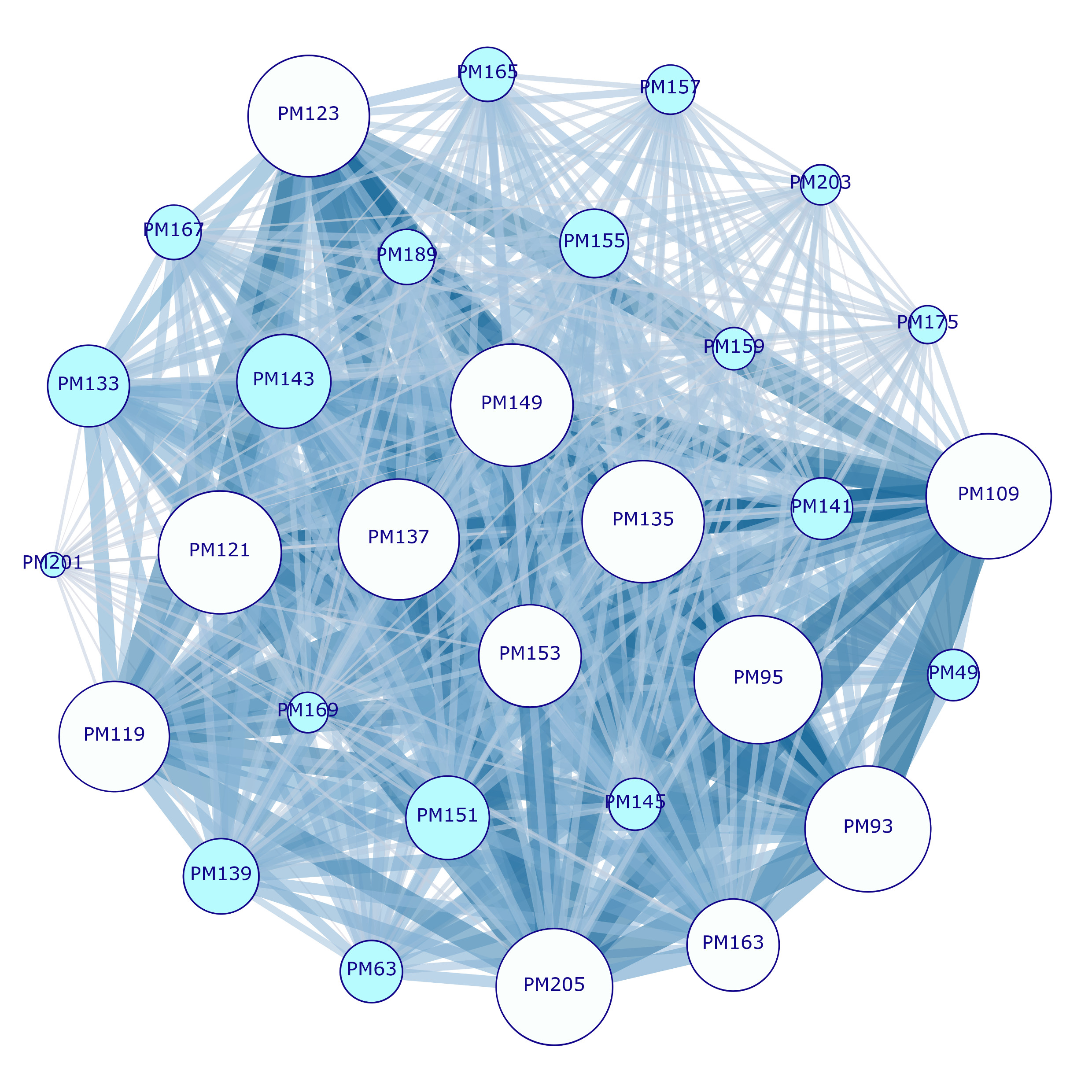
Figure 6: $G^{PM}_{3}(V_{3b},E_{3b})$ features graph. Each vertex correspond to one VOC. Edges thickness is proportional to the amount of shared species. Nodes dimensions are proportional to their weighted degree. The most interconnected VOCs are evident (lighter color): PM$93$ (Tp-f), PM$95$ (STp-f), PM$109$ (Tp-f), PM$121$ (Tp-f), PM$123$ (Tp/STp-f), PM$135$ (Tp/STp-f), PM$137$ (Tp/STp-f), PM$149$ (Tp/STp-f), PM$205$ (STp). The protonated mass PM$201$ (Tp), on the contrary, is the less interconnected node, thus turning out to be the less commonly shared emitted VOC.

The second bipartite projection of graph $G_{3}(V,E)$, i.e. the graph of VOCs $G^{PM}_{3}(V_{3b},E_{3b})$ is shown in Fig. 6. The graph is made up by $V_{3b}=30$ vertices (each corresponding to one protonated mass), and $E_{3b}=435$ edges. Usually a bipartite graph is based on the representation of different individuals according to the common properties they share. Here the emitted VOCs are the analogous of features, since the most two plants emit the same volatiles the most they are similar. We chose to show only the results coming from the second bipartite projection of graph $G_{3}(V,E)$, since we obtained similar results for $G_{2}(V,E)$. Graph $G_{1}(V,E)$ is not considered since from the previous analyses it turned out to be less suitable to describe data as a network. Colors here help the reader to distinguish between the most and less interconnected VOCs. Such as for the species-based bipartite projection graph, some protonated masses are highly connected with their neighborhoods. The highest value of weighted degree is recorded for PM$95$ ($s_{max}=679$), followed by PM$93$, PM$109$, PM$121$, PM$149$, PM$135$, PM$123$, PM$137$, PM$205$ (light blue vertices in Fig. 6). All that VOCs are shared by a large number of species, and they are terpenes compounds; accordingly, they are the responsible for the species grouping in the first two communities of graph $G^{P}_{3}(V_{3},E_{3})$ (aqua and yellow clusters in Fig. 5), made up by species rich in such types of compounds. Indeed, terpenes are the largest and assorted group of plant natural products, including hemiterpenes (C₅), monoterpenes (C₁₀), sesquiterpene (C₁₅), homoterpenes (C₁₁ and C₁₆), some diterpene (C₂₀) and triterpene (C₃₀), that are easily released into the atmosphere. The highest amount of species shared between two VOCs is observed between all the following couples of VOCs: PM$93$–PM$95$ and PM$93$–PM$109$ (respectively $48$ and $46$ maximum numbers of species), PM$95$–PM$109$, PM$109$–PM$137$, PM$93$–PM$121$, PM$95$–PM$121$, PM$95$–PM$135$, PM$95$–PM$137$, PM$95$–PM$149$, PM$109$–PM$121$, PM$93$–PM$123$. Their corresponding links are the thickest ones (highest link weights) in Fig. 6. In most cases, plants share two compounds belonging to the same chemical class; for example, PM$95$–PM$109$ is a couple of sesquiterpenes and/or sesquiterpenes fragments, while PM$93$–PM$123$ are terpenes and/or terpenes fragments. It’s worth noting that sesquiterpenes have a distinct biochemical pathway from that of other hemiterpenes[44], thus it is more expectable that a plant species emits, simultaneously, two or more VOCs of the same class instead of the combination of VOCs of different classes. However, terpenes biosynthesis is very complex[45] and uses many separated pathways, and cases of plants producing isoprene (terpenes building unit) but not other monoterpenes (and viceversa) have been frequently reported[46].

On the contrary, the two sulphur compounds PM$49$ and PM$63$, which considerably determine the assembling of the violet cluster in Fig. 5, are small dimension nodes, since the species they share are homogeneous in term of family composition, but they are few. Among volatile organic sulfur compounds, dimethylsulfide (DMS, PM$63$) and methanethiol (MT, PM$49$) are two of the most frequent products of plant metabolism. Their biosynthetic pathways share the role of a common lyase enzyme (dimethylsulfoniopropionate, DMSP) that is not widely distributed in terrestrial plants[47].

Finally, PM$201$ (Tp), PM$169$ (aldehydes, Ald, a product of monoterpene oxidation), and PM$159$ (acids/esters, Ac/Es) are some of the less interconnected VOCS.

Conclusions

Volatile organic compounds (VOCs), that represent a crucial component of a plant’s phenotype[3], have been analysed by bipartite networks methodology in order to classify plants species. In particular, several quantitative measures coming from Complex Network Theory[23, 24, 25] have been applied to uncover eventual similarities between the species in term of their VOCs emissions. To assure the reliability and robustness of the results, different classical and advanced community detection algorithms have been applied, and only the comparable results were retained. Moreover data have been pre-processed by means of both descriptive and quantitative statistical methods, to better focus on data behaviour. VOCs time series, obtained by recording the emissions content for each available species, suggest the presence of spike-like pulses (corresponding to few species), exceeding from a quite flat background signal. Each VOC turns out to be emitted by few species in a very large quantity, with respect to all the other species emissions of the same protonated mass.

After a preliminary test performed on the whole dataset, some VOCs have been excluded. In fact, some volatiles, especially C6 compounds and acetaldehyde, can occur in response to external stress, including wounding; this should be taken into account when using these compounds for communities detection analysis. Using a reduced dataset, community detection suggested the presence of $4$ clusters. Two communities are made up by highly VOCs-emitting species. We recall here the most interconnected nodes: Lavandula spica L. (Lavender), Foeniculum vulgare Mill. (Fennel), Santolina chamaecyparissus L. (Cotton lavender), Crithmum maritimum L. (Samphire), Cupressus sempervirens L. (Mediterranean cypress), Ocimum basilicum L. (Basil) (for cluster $1$); Citrus x Aurantium L. (Bitter orange), Cannabis sativa L. (Hemp), Citrus x Limon L. (Lemon), Humulus lupulus L. var. Cascade (Common hop), Ruta graveolens L. (Rue), Calycanthus floridus L. (Carolina allspice) and Psidium guajava L. (guava) (for cluster $2$). A third community clearly groups species belonging to $Brassicaceae$ family, turning out to be quite homogeneous in terms of clusters families composition. Finally, a fourth community highlights all those species which, by network construction, are not sharing any VOCs emission with the other species. See previous Section “Community detection analysis” for more details.

The second bipartite projection confirmed terpenes compounds and sulphur compounds to be the two chemical classes most responsible for species classification. Indeed, the chemistry of volatiles has been shown to be species-specific[44]; for example, species characterized by terpenes and nitrogen-containing compounds as floral volatiles are different from species releasing sulphur-containing volatiles[48]. Moreover, terpenes compounds emitted by plant species (the so-called “terpenome”[49]), are the major constituents of plants essential oils[50], and can be used to distinguish different species; in this study, although the exact chemical definition of the compounds involved is beyond the purpose, community detection highlighted two well defined groups (clusters $1$ and $2$) of species that emit different terpenes compounds. In conclusion, complex network analysis confirms to be an advantageous methodology to uncover plants relationships also related to the way they react to the environment in which they live. That result strengthens previous findings obtained by applying Complex Network Theory to the plants morphological features[33]. A similar approach can be extended to different fields in botanic framework, such as plant ecology, psychophysiology and plant communication.

Methods

Data

PTR-ToF-MS has been used in this study as the detector for the organic compounds emitted by leaf samples. A full description of this tool, with its advantages and disadvantages, can be found elsewhere[51, 52, 53]. The compounds emitted by different leaves were transported from the air stream where collided with H₃O⁺ reagent ion inside the drift tube. The analysis was carried out as follows: each leaf samples was placed into $3/4$ L glass jar (Bormioli, Italy) provided of glass stopper fitted with two Teflon tubes connected respectively to the PTR-ToF-MS ($8000$, Ionicon Analitic GmbH, Innsbruck, Austria) and the zero air generator (Peak Scientific instruments, USA). Each sample was obtained by cutting pieces of representative mature and healthy leaves from three different plant exemplars ($5$ g total weight). For each plant species, three replicates (three different jar) were evaluated. An overview of the plants used is shown in Tab 3 and Tab 5, for a total of $109$ species belonging to $56$ plant families. Before each leaf sample analysis, the glass jar was exposed to $1$ minute of purified air flux ($100$ sccm) to remove all the VOCs accumulated in the head space during the time between sample preparation; then, a blank air sample was taken and subsequently used for background correction. All measurements were conducted in an air-conditioned room, with temperature and humidity respectively set at $20\pm 3^{\circ}$C and 65% [54], and using the same PTR-ToF-MS instrumental parameters: drift pressure = $2.30$ mbar, drift temperature = $60^{\circ}$C and inlet temperature = $40^{\circ}$C, drift voltage = $600$ V, extraction voltage at the end of the tube (Udx) $35$ V, which resulted in E/N ratio of $140$ Td ($1$ Td $=10-17$ Vcm^-2). This setup allowed a good balance between excessive water cluster formation and product ion fragmentation[55]. Moreover, the inlet flux was set to $100$ sscm. The internal calibration of ToF spectra was based on m/z $=29.997$ (NO⁺), m/z $=59.049$ (C₃H₇O⁺) and m/z = $137.132$ (C₁₀H${}_{17}^{+}$) and was performed off-line after dead time correction; for peak quantification, the resulting data were corrected according to the duty cycle. Data were recorded with the software TOF-DAQ (Tofwerk AG, Switzerland), the sampling time for each channel of TOF acquisition was 0.1 ns, acquiring 1 spectrum per second, for a mass spectrum range between m/z $20$ and m/z $220$. The raw data were normalized to the primary ion signal from counts per seconds (cps) to normalized counts per second (ncps) as described by Herbig et al.[56]. Data were filtered following the procedure used by Taiti et al.[57] and used for statistical analysis. In this manner, a dataset comprised of mean mass spectra for each sample analyzed was compiled. Finally, the tentative identifications of peaks was performed on the basis of an high mass resolution and rapid identification of compounds with a high level of confidence[58]. Further characterization of VOCs belonging to certain chemical classes such as terpenes, which are prone to fragmentation, was attempted using literature data on fragmentation of standards during PTR-ToF-MS analysis [59, 60, 61]. Similar approach was performed for the other identified compound, e.g. following Papurello et al.[62] and Liu et al.[63] for sulfur compounds, Loreto et al.[36], Brilli et al.[37], Degen et al.[38], and Wu et al.[39] for wounding-related VOCs, and Schwartz et al.[64] and Soukoulis et al.[65] for aldehydes, ketones and alcohols.

Descriptive statistics: boxplots

Boxplots are an intuitive graphical non-parametric method particularly suitable to visualize the distribution of continuous univariate data, firstly proposed by Tukey[34]. None a-priory assumption is made on the underlying statistical distribution. Boxplots show information about data location and spread, by starting from the estimation of the second quartile (or median, $Q_{2}$) and of the interquartile range ($IQR$), where $IQR=Q_{3}-Q_{1}$, and $Q_{3}$ and $Q_{1}$ are the third and first quartiles, respectively. Boxplots are also known as box-and-whisker plots. The rectangular box is related to the data quartiles, and, more in details, the left and right sides of the rectangle correspond respectively to $Q_{1}$ and $Q_{3}$. The whiskers are lines extending from the box till lower and upper first outliers. It follows that the boxplot width visually shows the sample $IQR$, the vertical band drawn inside the box represents the median, and as a whole the box is a measure of the data dispersion and skewness. On the contrary, there is no common definition for the end of the boxplots whiskers. In the present work we adopt the following formalism: outliers are defined as those data points lying outside the range ($Q_{1}-1.5\times IQR$; $Q_{3}+1.5\times IQR$); extreme events are defined as those data points exceeding the range ($Q_{1}-3\times IQR$; $Q_{3}+3\times IQR$). Several graphical solutions for boxplots are present nowadays, and generalized versions allow to apply them to skewed distributions, also, by assuring a robust measure of the skewness in the determination of the whiskers[35]. We recall here that the quartiles are also called quantiles of order $1/4$, $1/2$, $3/4$, or $Q_{\frac{1}{4}}$, $Q_{\frac{1}{2}}$, and $Q_{\frac{3}{4}}$, respectively. That second formalism will be used along the paper.

Building the graph: projection in the space of plants/VOCs

Data are represented as an undirected bipartite graph $G(N,E)$, where every plant species $p$ is connected to its features, i.e. in that case the VOCs it emits. No connection is present between the two set of nodes, i.e. the plant species and the recorded VOCs. Usually, a bipartite graph can also be described by a binary matrix $A(p,f)$ whose element $a_{ij}$ is $1$ just if plant $p$ shows the feature $f$. The most immediate way to measure correlation between species is counting how many VOCs the plants species share in term of significant emissions, and similarly how many plants emit the same VOCs. We refer to the Basic Network Analysis subsection for a proper description of the methodology. In formulas, this corresponds to consider the matrix of species $P(p,p)=AA^{T}$ and the matrix of volatile organic compounds, $F(f,f)=A^{T}A$, i.e. the two bipartite projections of $G(N,E)$. In the present work, we focused on the graph having as nodes the different plants, i.e. on the Plants graph $G^{P}(N,E)$ whose edges weights are proportional to the number of commonly emitted VOCs between plants. Second, in order to catch the predominant similarities in terms of volatile organic compounds emissions, we analysed the second bipartite projection, i.e. the Features graph, $G^{F}(N,E)$, whose nodes represent the emitted VOCs. In that case edges weights were proportional to the number of plants sharing the same emitted compound.

Basic network analysis

As regards network analysis, we computed some global and local basic metrics described hereafter.

• Graph density ($D$) is defined as the ratio between the numbers of existing edges and the possible number of edges. Given a $N$-order network, graph density is computed as $D=\frac{2E}{N(N-1)}$. Strictly connected to $D$, is the graph average degree $\overline{k}=\frac{1}{V}\sum_{i=1}^{V}k_{i}=\frac{2E}{V}$, where $k_{i}$ is the degree of each vertex in $V$, i.e. the number of edges incident to it.

• Network clustering coefficient ($c$) is the overall measure of clustering in a undirected graph in terms of probability that the adjacent vertices of a vertex are connected. More intuitively, global clustering coefficient is simply the ratio of the triangles and the connected triples in the graph. The corresponding local metric is the local clustering coefficient, which is the tendency among two vertices to be connected if they share a mutual neighbour. In this analysis we used a local vertex-level quantity[20] defined in Eq. (1):

  $$c_{i}^{w}=\frac{1}{s_{i}(k_{i}-1)}\sum_{jh}\frac{(w_{ij}+w_{ih})}{2}a_{ij}a_{ih}a_{jh},$$ (1)

  The normalization factor $\frac{1}{s_{i}(k_{i}-1)}$ accounts for the weight of each edge times the maximum possible number of triplets in which it may participate, and it ensures that $0\leq c_{i}^{w}\leq 1$. That metric combines the topological information with the weight distribution of the network, and it is a measure of the local cohesiveness, grounding on the importance of the clustered structure evaluated on the basis of the amount of interaction intensity actually found on the local triplets[20].

• Network strength ($s$) is obtained by summing up the edge weights of the adjacent edges for each vertex[20]. That metric is a more significant measure of the network properties in terms of the actual weights, and is obtained by extending the definition of vertex degree $k_{i}=\sum_{j}a_{ij}$, with $a_{ij}$ elements of the network adjacent matrix A. In formulas, $s_{i}=\sum_{j=1}^{N}a_{ij}w_{if}$.

Grouping plants from graph: communities detection analysis

Communities detection aims essentially at determine a finite set of categories (clusters or communities) able to describe a data set, according to similarities among its objects[66]. More in general, hierarchy is a central organising principle of complex networks, able to offer insight into many complex network phenomena[67]. In the present work we adopted the following methods belonging to complex networks framework:

• Fast greedy (FG) hierarchical agglomeration algorithm[68] is a faster version of the previous greedy optimisation of modularity[22]. FG gives identical results in terms of found communities. However, by exploiting some shortcuts in the optimisation problem and using more sophisticated data structures, it runs far more quickly, in time $O(md\log n)$, where $d$ is the depth of the “dendrogram” describing the network community structure.

• Walktrap community finding algorithm (WT) finds densely connected subgraphs from a undirected locally dense graph via random walks. The basic idea is that short random walks tend to stay in the same community[69]. Starting from this point, $WT$ is a measure of similarities between vertices based on random walks, which captures well the community structure in a network, working at various scales. Computation is efficient and the method can be used in an agglomerative algorithm to compute efficiently the community structure of a network.

• Louvain or Blondel method (BL) [70] to uncover modular communities in large networks requiring a coarse-grained description. Louvain method ($BL$) is an heuristic approach based on the optimisation of the modularity parameter ($Q$) to infer hierarchical organization. Modularity (Eq. (2)) measures the strength of a network division into modules[22, 71], as it follows:

  $$Q=\frac{1}{2m}\sum_{vw}\left[A_{vw}-\frac{k_{v}k_{w}}{\left(2m\right)}\right]\delta\left(c_{v},c_{w}\right)=\sum^{c}_{i=1}(e_{ii}-a^{2}_{i}),$$ (2)

  where, $e_{ii}$ is the fraction of edges which connect vertices both lying in the same community $i$, and $a_{i}$ is the fraction of ends of edges that connect vertices in community $i$, in formulas: $e_{ii}=\frac{1}{2m}\sum_{vw}\left[A_{vw}\delta\left(c_{v},c_{w}\right)\right]$, and $a_{i}=\frac{k_{i}}{2m}=\sum_{i}e_{ij}$; A is the adjacent matrix for the network; $c$ the number of communities; $k_{i}=\sum_{w}A_{vw}$ the degree of the vertex-$i$, $n$ and $m=\frac{1}{2}\sum_{vw}A_{vw}$ the number of graph vertices and edges, respectively. Delta function, $\delta(i,j)$, is $1$ if $i=j$, and 0 otherwise.

• Label propagation (LP) community detection method is a fast, nearly linear time algorithm for detecting community structure in networks[21]. Vertices are initialised with a unique label and, at every step, each node adopts the label that most of its neighbours currently have, that is by a process similar to an ‘updating by majority voting’ in the neighbourhood of the vertex. Moreover, $LP$ uses the network structure alone to run, without requiring neither optimisation of a predefined objective function nor a-priori information about the communities, thus overcoming the usual big limitation of having communities which are implicitly defined by the specific algorithm adopted, without an explicit definition. In this iterative process densely connected groups of nodes form a consensus on a unique label to form communities.

Besides the complex networks communities detection methodologies, a classic cluster analysis[72, 73] based on dimensionality reduction methods was also performed to assure the results robustness and reliability, by rejecting those solutions not independent from the statistical methodology applied.

Author contributions statement

GV, EM, CT, GC and SM contributed equally to the analysis of the dataset and to the interpretation of the results of this analysis, both from the point of view of Network Theory as well as in terms of biological implications. They also contributed equally to the writing and reviewing of the manuscript.

Additional information

Competing financial interests. The authors declare no competing financial interests.

References

- [1] Theis, N. & Lerdau, M. The evolution of function in plant secondary metabolites. International Journal of Plant Sciences 164, S93–S102 (2003).
- [2] Pichersky, E. & Gang, D. R. Genetics and biochemistry of secondary metabolites in plants: an evolutionary perspective. Trends in plant science 5, 439–445 (2000).
- [3] Dicke, M. & Loreto, F. Induced plant volatiles: from genes to climate change. Trends in plant science 15, 115 (2010).
- [4] Dudareva, N., Negre, F., Nagegowda, D. A. & Orlova, I. Plant volatiles: recent advances and future perspectives. Critical reviews in plant sciences 25, 417–440 (2006).
- [5] Peñuelas, J. & Llusia, J. The complexity of factors driving volatile organic compound emissions by plants. Biologia Plantarum 44, 481–487 (2001).
- [6] Holopainen, J. K., Heijari, J., Oksanen, E. & Alessio, G. A. Leaf volatile emissions of betula pendula during autumn coloration and leaf fall. Journal of chemical ecology 36, 1068–1075 (2010).
- [7] Holopainen, J. K. & Gershenzon, J. Multiple stress factors and the emission of plant vocs. Trends in plant science 15, 176–184 (2010).
- [8] Spinelli, F., Cellini, A., Piovene, C., Nagesh, K. M. & Marchetti, L. Emission and function of volatile organic compounds in response to abiotic stress (INTECH Open Access Publisher, 2011).
- [9] Mumm, R., Schrank, K., Wegener, R., Schulz, S. & Hilker, M. Chemical analysis of volatiles emitted by pinus sylvestris after induction by insect oviposition. Journal of chemical ecology 29, 1235–1252 (2003).
- [10] Dudareva, N. & Pichersky, E. Biochemical and molecular genetic aspects of floral scents. Plant physiology 122, 627–634 (2000).
- [11] Baldwin, I. T., Halitschke, R., Paschold, A., Von Dahl, C. C. & Preston, C. A. Volatile signaling in plant-plant interactions:” talking trees” in the genomics era. Science 311, 812–815 (2006).
- [12] Heil, M. & Karban, R. Explaining evolution of plant communication by airborne signals. Trends in ecology & evolution 25, 137–144 (2010).
- [13] War, A. R. et al. Mechanisms of plant defense against insect herbivores. Plant signaling & behavior 7, 1306–1320 (2012).
- [14] Ruuskanen, T. et al. Measurements of Volatile Organic Compounds-from Biogenic Emissions to Concentrations in Ambient Air. Ph.D. thesis, University of Helsinki, Faculty of Science, Department of Physics, Division of Atmospheric Sciences and Geophysics (2009).
- [15] Agrawal, A. A. Current trends in the evolutionary ecology of plant defence. Functional Ecology 25, 420–432 (2011).
- [16] Berenbaum, M. R. & Zangerl, A. R. Facing the future of plant-insect interaction research: le retour à la ”raison d’être”. Plant Physiology 146, 804–811 (2008).
- [17] Llusia, J., Penuelas, J. & Gimeno, B. Seasonal and species-specific response of voc emissions by mediterranean woody plant to elevated ozone concentrations. Atmospheric Environment 36, 3931–3938 (2002).
- [18] Caldarelli, G. Scale-Free Networks: complex webs in nature and technology. OUP Catalogue (2007).
- [19] Boccaletti, S., Latora, V., Moreno, Y., Chavez, M. & Hwang, D. U. Complex networks: Structure and dynamics. Physics Reports 424, 175 – 308 (2006). URL http://www.sciencedirect.com/science/article/pii/S037015730500462X.
- [20] Barrat, A., Barthelemy, M., Pastor-Satorras, R. & Vespignani, A. The architecture of complex weighted networks. Proceedings of the National Academy of Sciences of the United States of America 101, 3747–3752 (2004).
- [21] Raghavan, U. N., Albert, R. & Kumara, S. Near linear time algorithm to detect community structures in large-scale networks. Physical Review E 76, 036106 (2007).
- [22] Newman, M. E. & Girvan, M. Finding and evaluating community structure in networks. Physical review E 69, 026113 (2004).
- [23] Ma, J., Shi, Y., Wang, Z. & Yue, J. On wiener polarity index of bicyclic networks. Scientific reports 6 (2016).
- [24] Li, X., Li, Y., Shi, Y. & Gutman, I. Note on the homo-lumo index of graphs. MATCH Commun. Math. Comput. Chem 70, 85–96 (2013).
- [25] Cao, S., Dehmer, M. & Shi, Y. Extremality of degree-based graph entropies. Information Sciences 278, 22–33 (2014).
- [26] Dunne, J. A., Williams, R. J. & Martinez, N. D. Food-web structure and network theory: The role of connectance and size. Proceedings of the National Academy of Sciences 99, 12917–12922 (2002). URL http://www.pnas.org/content/99/20/12917.abstract. http://www.pnas.org/content/99/20/12917.full.pdf.
- [27] Stelzl, U. et al. A human protein-protein interaction network: A resource for annotating the proteome. Cell 122, 957 – 968 (2005). URL http://www.sciencedirect.com/science/article/pii/S0092867405008664.
- [28] Proulx, S. R., Promislow, D. E. & Phillips, P. C. Network thinking in ecology and evolution. Trends in Ecology & Evolution 20, 345–353 (2005).
- [29] Barabási, A.-L., Gulbahce, N. & Loscalzo, J. Network medicine: a network-based approach to human disease. Nature Reviews Genetics 12, 56–68 (2011).
- [30] Lee, D.-S. et al. The implications of human metabolic network topology for disease comorbidity. Proceedings of the National Academy of Sciences of the United States of America 105, 9880–9885 (2008).
- [31] Stephan, K. E. et al. Computational analysis of functional connectivity between areas of primate cerebral cortex. Philosophical Transactions of the Royal Society of London B: Biological Sciences 355, 111–126 (2000).
- [32] Caretta Cartozo, C., Garlaschelli, D., Ricotta, C., M., B. & G., C. Quantifying the universal taxonomic diversity in real species assemblage. Journal of Physics A 41, 224012 (2008).
- [33] Vivaldo, G., Masi, E., Pandolfi, C., Mancuso, S. & Caldarelli, G. Networks of plants: how to measure similarity in vegetable species. arXiv preprint arXiv:1602.05887 (2016).
- [34] Tukey, J. Exploratory data analysis.-reading, mass.: Addison-wesley. Exploratory data analysis: Reading, Mass: Addison-Wesley (1977).
- [35] Vandervieren, E. & Hubert, M. An adjusted boxplot for skewed distributions. COMPSTAT 2004, proceedings in computational statistics. Springer, Heidelberg 1933–1940 (2004).
- [36] Loreto, F., Barta, C., Brilli, F. & Nogues, I. On the induction of volatile organic compound emissions by plants as consequence of wounding or fluctuations of light and temperature. Plant, cell & environment 29, 1820–1828 (2006).
- [37] Brilli, F. et al. Detection of plant volatiles after leaf wounding and darkening by proton transfer reaction ’time-of-flight’ mass spectrometry (ptr-tof). PLoS One 6, e20419 (2011).
- [38] Degen, T., Dillmann, C., Marion-Poll, F. & Turlings, T. C. High genetic variability of herbivore-induced volatile emission within a broad range of maize inbred lines. Plant physiology 135, 1928–1938 (2004).
- [39] Wu, J., Hettenhausen, C., Schuman, M. C. & Baldwin, I. T. A comparison of two nicotiana attenuata accessions reveals large differences in signaling induced by oral secretions of the specialist herbivore manduca sexta. Plant Physiology 146, 927–939 (2008).
- [40] Van Langenhove, H. J., Cornelis, C. P. & Schamp, N. M. Identification of volatiles emitted during the blanching process of brussels sprouts and cauliflower. Journal of the Science of Food and Agriculture 55, 483–487 (1991).
- [41] Geervliet, J. B., Posthumus, M. A., Vet, L. E. & Dicke, M. Comparative analysis of headspace volatiles from different caterpillar-infested or uninfested food plants of pieris species. Journal of chemical ecology 23, 2935–2954 (1997).
- [42] Buhr, K., van Ruth, S. & Delahunty, C. Analysis of volatile flavour compounds by proton transfer reaction-mass spectrometry: fragmentation patterns and discrimination between isobaric and isomeric compounds. International Journal of Mass Spectrometry 221, 1–7 (2002).
- [43] Pierre, P. S. et al. Differences in volatile profiles of turnip plants subjected to single and dual herbivory above-and belowground. Journal of chemical ecology 37, 368–377 (2011).
- [44] Dudareva, N., Klempien, A., Muhlemann, J. K. & Kaplan, I. Biosynthesis, function and metabolic engineering of plant volatile organic compounds. New Phytologist 198, 16–32 (2013).
- [45] Sun, P., Schuurink, R. C., Caissard, J.-C., Hugueney, P. & Baudino, S. My way: Noncanonical biosynthesis pathways for plant volatiles. Trends in Plant Science (2016).
- [46] Lindfors, V. & Laurila, T. Biogenic volatile organic compound (voc) emissions from forests in finland. Boreal environment research 5, 95–113 (2000).
- [47] Bentley, R. & Chasteen, T. G. Environmental voscs—-formation and degradation of dimethyl sulfide, methanethiol and related materials. Chemosphere 55, 291–317 (2004).
- [48] Dobson, H. E. Relationship between floral fragrance composition and type of pollinator. Biology of floral scent 147–198 (2006).
- [49] Kumari, S. et al. Essoildb: a database of essential oils reflecting terpene composition and variability in the plant kingdom. Database 2014, bau120 (2014).
- [50] Edris, A. E. Pharmaceutical and therapeutic potentials of essential oils and their individual volatile constituents: a review. Phytotherapy research 21, 308–323 (2007).
- [51] Lindinger, W. & Jordan, A. Proton-transfer-reaction mass spectrometry (ptr–ms): on-line monitoring of volatile organic compounds at pptv levels. Chemical Society Reviews 27, 347–375 (1998).
- [52] Jordan, A. et al. A high resolution and high sensitivity proton-transfer-reaction time-of-flight mass spectrometer (ptr-tof-ms). International Journal of Mass Spectrometry 286, 122–128 (2009).
- [53] Taiti, C. et al. Assessing voc emission by different wood cores using the ptr-tof-ms technology. Wood Science and Technology 1–23.
- [54] Mancuso, S. et al. Soil volatile analysis by proton transfer reaction-time of flight mass spectrometry (ptr-tof-ms). Applied Soil Ecology 86, 182–191 (2015).
- [55] Pang, X. Biogenic volatile organic compound analyses by ptr-tof-ms: Calibration, humidity effect and reduced electric field dependency. Journal of Environmental Sciences 32, 196–206 (2015).
- [56] Herbig, J. et al. On-line breath analysis with ptr-tof. Journal of breath research 3, 027004 (2009).
- [57] Taiti, C. et al. Sometimes a little mango goes a long way: A rapid approach to assess how different shipping systems affect fruit commercial quality. Food analytical methods 9, 691–698 (2016).
- [58] Lanza, M. et al. Selective reagent ionisation-time of flight-mass spectrometry: a rapid technology for the novel analysis of blends of new psychoactive substances. Journal of Mass Spectrometry 50, 427–431 (2015).
- [59] Maleknia, S. D., Bell, T. L. & Adams, M. A. Ptr-ms analysis of reference and plant-emitted volatile organic compounds. International Journal of Mass Spectrometry 262, 203–210 (2007).
- [60] Kim, S. et al. Measurement of atmospheric sesquiterpenes by proton transfer reaction-mass spectrometry (ptr-ms). Atmospheric Measurement Techniques 2 (2009).
- [61] Demarcke, M. et al. Laboratory studies in support of the detection of sesquiterpenes by proton-transfer-reaction-mass-spectrometry. International Journal of Mass Spectrometry 279, 156–162 (2009).
- [62] Papurello, D. et al. Monitoring of volatile compound emissions during dry anaerobic digestion of the organic fraction of municipal solid waste by proton transfer reaction time-of-flight mass spectrometry. Bioresource technology 126, 254–265 (2012).
- [63] Liu, D., Andreasen, R. R., Poulsen, T. G. & Feilberg, A. Experimental determination of mass transfer coefficients of volatile sulfur odorants in biofilter media measured by proton-transfer-reaction mass spectrometry (ptr-ms). Chemical engineering journal 219, 335–345 (2013).
- [64] Schwarz, K., Filipiak, W. & Amann, A. Determining concentration patterns of volatile compounds in exhaled breath by ptr-ms. Journal of Breath Research 3, 027002 (2009).
- [65] Soukoulis, C. et al. Ptr-tof-ms, a novel, rapid, high sensitivity and non-invasive tool to monitor volatile compound release during fruit post-harvest storage: the case study of apple ripening. Food and Bioprocess Technology 6, 2831–2843 (2013).
- [66] Campello, R. A Fuzzy Extension of the Rand Index and Other Related Indexes for Clustering and Classification Assessment. Pattern Recognition Letters, 28 (2007).
- [67] Clauset, A., Moore, C. & Newman, M. Hierarchical structure and the prediction of missing links in networks. Nature 453, 98–101 (2008). URL http://dx.doi.org/10.1038/nature06830.
- [68] Clauset, A., Newman, M. E. & Moore, C. Finding community structure in very large networks. Physical review E 70, 066111 (2004).
- [69] Pons, P. & Latapy, M. Computing communities in large networks using random walks. In Computer and Information Sciences-ISCIS 2005, 284–293 (Springer, 2005).
- [70] Blondel, V. D., Guillaume, J.-L., Lambiotte, R. & Lefebvre, E. Fast unfolding of communities in large networks. Journal of Statistical Mechanics: Theory and Experiment 2008, P10008 (2008). URL http://stacks.iop.org/1742-5468/2008/i=10/a=P10008.
- [71] Newman, M. E. Fast algorithm for detecting community structure in networks. Physical review E 69, 066133 (2004).
- [72] Jolliffe, I. Principal component analysis (Wiley Online Library, 2002).
- [73] MacQueen, J. et al. Some methods for classification and analysis of multivariate observations. In Proceedings of the fifth Berkeley symposium on mathematical statistics and probability, vol. 1, 281–297 (Oakland, CA, USA., 1967).