High-Dimensional Variable Selection and Prediction under Competing Risks with Application to SEER-Medicare Linked Data

Abstract

Competing risk analysis considers event times due to multiple causes, or of more than one event types. Commonly used regression models for such data include 1) cause-specific hazards model, which focuses on modeling one type of event while acknowledging other event types simultaneously; and 2) subdistribution hazards model, which links the covariate effects directly to the cumulative incidence function. Their use and in particular statistical properties in the presence of high-dimensional predictors are largely unexplored. Motivated by an analysis using the linked SEER-Medicare database for the purposes of predicting cancer versus non-cancer mortality for patients with prostate cancer, we study the accuracy of prediction and variable selection of existing statistical learning methods under both models using extensive simulation experiments, including different approaches to choosing penalty parameters in each method. We then apply the optimal approaches to the analysis of the SEER-Medicare data.

^a Altman Clinical and Translational Research Institute, University of California, San Diego, CA 92093, U.S.A
^b Department of Radiation Medicine and Applied Sciences, University of California, San Diego, CA 92093, U.S.A
^c Department of Family Medicine and Public Health and Department of Mathematics, University of California, San Diego, CA 92093, U.S.A
^* Corresponding author

1 Introduction

As an illustration project of how information contained in patients’ electronic medical records can be harvested for the purposes of precision medicine, we consider the large data set linking the Surveillance, Epidemiology and End Results (SEER) Program database of the National Cancer Institute with the federal health insurance program Medicare database for prostate cancer patients of age 65 or older. Each year 180,000 men are diagnosed with prostate cancer in the US, and the important clinical decision commonly encountered in this patient population is whether to pursue aggressive cancer-directed therapy in the presence of pre-existing comorbidities. Prostate cancer can progress slowly, and a proportion of men will die of competing causes before their prostate cancer becomes symptomatic. Current clinical guidelines for the management of prostate cancer instruct clinicians to make treatment decisions based on two factors: 1) an estimation of the aggressiveness of a patient’s tumor; and 2) estimation of a patient’s overall life expectancy [26]. Classical cancer-specific survival prediction relies on three main risk factors: tumor stage, Gleason score, and prostate specific antigen (PSA). On the other hand, currently no tool exists to predict non-cancer survival for this patient population. As non-cancer and cancer survival are not independent, i.e. so-called competing risks in the statistical literature, an accurate comprehensive survival prediction tool should consider both types of risks simultaneously.

Competing risks occur when multiple types of failures co-exist and the occurrence of one type of failure may prevent the observation of the other types of failure. In addition the failure times may be subject to right-censoring. In the regression settings the Cox proportional hazards model can be used to model the so-called cause-specific hazards, and existing software for fitting the Cox model for classical survival data without competing risks can be used to fit the proportional cause-specific hazards model [22]. Under this model, however, the dependence of the cumulative incidence function of a particular failure type on the covariates involves also the effects of the covariates on the cause-specific hazards of all other types of failures. Beyersmann et al. [1] showed as an example in patients receiving peripheral blood stem-cell transplantation, while the cause-specific hazard ratio for certain baseline risk factors of bloodstream infection (competing with the event of neutropenia) might be similar, the corresponding cumulative incidence functions can be quite different.

In order to link the covariates directly to the cumulative incidence functions (CIF), Fine and Gray [11] proposed to model the subdistribution hazards. The proportional hazards modeling of the subdistribution hazards, also known as Fine-Gray model, has gained popularity in recent years. The proportional cause-specific hazards model, and the proportional subdistribution hazards model are typically not valid at the same time, and limited empirical experiences seem to indicate that in real data applications the two models can lead to similar conclusions [18].

We restrict our analysis to patients diagnosed between 2004 and 2009 in the SEER-Medicare database. After excluding additional patients with missing clinical records, we have a total of 57,011 patients who have information available on 7 relevant clinical variables (age, PSA, Gleason score, AJCC stage, and AJCC stage T, N, M, respectively), 5 demographical variables (race, marital status, metro, registry and year of diagnosis), plus 8971 binary insurance claim codes. We assumed that the survival prediction would occur at the time of diagnosis, therefore we used clinical and demographic information at the time of diagnosis, and insurance claims data during the year prior to diagnosis. Insurance claims capture medical diagnoses and procedures through HCPCS codes, ICD-9 diagnosis codes, and ICD-9 procedure codes. These claims indirectly describe events that occur in surgical procedures, hospitalization and outpatient activities. We converted each unique insurance claim code into a binary variable denoted 1 if the claim appeared anytime in the year before diagnosis, and 0 if the code was absent. Until December 2013 (end of follow-up for this data) there were a total of 1,247 deaths due to cancer, and 5,221 deaths unrelated to cancer. It is well understood that for time-to-event data, the number of events dictates the effective sample size, so in this case we have more predictors to consider than the effective sample size.

Researchers have studied different approaches to analyze survival data with high dimensional covariates. Notably, Tibshirani [28] proposed the least absolute shrinkage and selection operator (LASSO) under the Cox proportional hazards model. Zhang and Lu [35] investigated the statistical properties of adaptive LASSO for the Cox proportional hazards model. Hothorn et al. [20] introduced a random forest algorithm and a generic gradient boosting algorithm for right-censoring data. When considering theoretical aspects, Bradic et al. [4] studied a group of penalty functions and established strong oracle properties of non-concave penalized methods for ultra high dimensional covariates in the presence of right-censoring. In comparison, very few high-dimensional methods have been developed in the presence of competing risks. Binder et al. [3] first proposed a boosting approach for fitting the proportional subdistribution hazards model. Very recently (published online at the time of submission of this manuscript) Fu et al. [15] considered penalized approaches under the same model. Given the high-dimensional nature of our data, in this paper we will consider both the proportional cause-specific hazards (PCSH) model and the proportional subdistribution hazards (PSDH) model, and investigate the accuracy of variable selection and prediction using existing computational software under either model. This leads to the Binder et al. approach under the PSDH model, and LASSO approach under the PCSH model, both being readily implemented and applicable to our large data set. Both approaches rely critically on the selection of a ‘penalty’ parameter, and there are different ways to select this parameter. We will empirically evaluate these different methods using Monte Carlo simulations. The ultimate goal is to assess the prediction accuracy of the cumulative incidence function as a risk assessment tool.

The remainder of this paper is organized as follows: in Section 2, we review the proportional cause-specific hazards model and the proportional subdistribution hazards model. In Section 3, we review the relevant statistical learning methods that have been or can be feasibly implemented to analyze competing risks data under each model. In Section 4, we conduct comprehensive simulation studies on these methods with varying numbers of predictors (relative to the sample size), that are continuous or binary (and in case of binary, sparse or not sparse). In Section 5, we apply the statistical learning methods under either model to classify prostate patients from the SEER-Medicare linked data into different risk groups according to their predicted cumulative incidence functions. Finally, Section 6 contains discussion and directions for future work.

2 Competing Risk Models

Let $\epsilon=1,...,J$ be the cause or type (we use the two words interchangeably in the following) of failure. Let $T=\min_{j=1}^{J}\tilde{T}_{j}$ denote the observed failure time if there is no censoring which is due to one of the causes, while failures from other types or causes are latent. Let $X_{i}=\min(T_{i},C_{i})$, $\delta_{i}=I(T_{i}\leq C_{i})$, where $C_{i}$ is the potential censoring time, and is assumed non-informative. Denote $S(t)=P(T>t)$ the survival function of $T$. The cumulative incidence function (CIF) for failure type $j$ is $F_{j}(t)=P(T\leq t,\epsilon=j)$. Obviously $S(t)=1-\sum_{j=1}^{J}F_{j}(t)$, and $\sum_{j=1}^{J}F_{j}(\infty)=1$. Denote the cause-specific hazard function of type $j$ as $\lambda_{j}(t)=\lim_{\Delta t\rightarrow 0+}Pr(t\leq T<t+\Delta t,J=j|T\geq t)/\Delta t$. Then one can also show that

$$F_{j}(t)=\int_{0}^{t}\lambda_{j}(u)S(u)du,$$ (1)

leading to a nonparametric estimate of the CIF if we use [12]:

$$\hat{\lambda}_{j}(t_{i}) = \frac{d_{ji}}{n_{i}}$$ (2)

where $d_{ji}$ denotes the number of failures from cause $j$ at time $t_{i}$ and ${n_{i}}$ the number of subjects at risk at $t_{i}$, and

$$\hat{S}(t) = \prod_{j:t_{i}\leq t}\bigg{(}1-\sum_{j=1}^{J}\hat{\lambda}_{j}(t_{i})\bigg{)}.$$ (3)

Then we have $\hat{F}_{j}(t)=\sum_{i:t_{i}\leq t}\hat{p}_{j}(t_{i})$, where $\hat{p}_{j}(t_{i})=\hat{\lambda}_{j}(t_{i})\hat{S}(t_{i}^{-})$. While $\hat{F}_{j}(t)$ is a complex function of the $\hat{\lambda}_{j}(t_{i})$’s, the $(1-\alpha)100\%$ pointwise (for each $t$) confidence intervals can calculated using the ‘Cuminc()’ function in the R package ‘mstate’.

2.1 The PCSH Model

Given a vector of covariates $Z$, under the proportional hazards assumption of the cause-specific hazard function we have

$$\lambda_{j}(t|Z)=\lambda_{0j}(t)\exp(\beta_{j}^{\prime}Z),$$ (4)

for $j=1,...,J$. To estimate $\beta_{j}$, we can use any software for the regular Cox model by treating all other types of events as if censored, one type of events at a time. This is because the (partial) likelihood for all event types factors into a separate likelihood function for each event type, and the likelihood function for each event type treats all other types of events as if censored.

To estimate the cumulative incidence function given $Z=z_{0}$, we have similar to the above nonparametric estimation:

$$\hat{F}_{j}(t) = \int_{0}^{t}\hat{S}(u;z_{0})d\hat{\Lambda}_{j}(u;z_{0})$$

$$= \sum_{i=1}^{n}\frac{\hat{S}(X_{i};z_{0})\delta_{ji}I(X_{i}\leq t)\exp(\hat{\beta}_{j}^{\prime}z_{0})}{\sum_{i^{\prime}=1}^{n}I(X_{i}\leq X_{i^{\prime}})\exp({\hat{\beta}_{j}^{\prime}Z_{i^{\prime}}})},$$

where $\hat{S}(u;z_{0})=\exp\{-\sum_{j=1}^{J}\hat{\Lambda}_{j}(u;z_{0})\}$, $\hat{\Lambda}_{j}(u;z_{0})=\hat{\Lambda}_{0j}(u)\exp(\hat{\beta_{j}}^{\prime}z_{0})$, and the baseline cumulative hazard $\hat{\Lambda}_{0j}(u)$ is a Breslow-type estimator [5]. Notice that in estimating the overall survival function $\hat{S}$ we need to fit the models for all event types, even if we are only interested in the CIF of type $j$.

A $(1-\alpha)100\%$ pointwise confidence interval can be computed following Cheng et al. [8]. We implemented an R package ‘CompetingRisk’ [21] to compute the above estimator of the CIF with its pointwise confidence intervals.

2.2 The PSDH Model

Gray [19] introduced the subdistribution hazard function as $\tilde{\lambda}_{j}(t)=-\frac{d}{dt}\log\{1-F_{j}(t)\}$. Under the proportional hazards assumption of the subdistribution hazard function for cause 1 we have [11]

$$\tilde{\lambda}_{1}(t|Z)=\tilde{\lambda}_{0}(t)\exp(\beta^{\prime}Z).$$ (6)

It is easy to see that model (6) provides a direct way to estimate the CIF of cause 1, so that there is no need to fit models for the other causes in order to estimate $\mbox{CIF}_{1}$.

Fine and Gray [11] proposed estimating equations for $\beta$. Geskus [17] further showed that these estimating equations can be solved using weighted Cox regression, i.e. software for the regular Cox model incorporating weights. The baseline subdistribution hazard is again estimated using a modified version of Breslow’s estimator. The $(1-\alpha)100\%$ pointwise confidence intervals can be constructed by sampling standard normal random variables and otherwise closed-form formulas [11].

3 Regularization

Classical statistical methods, such as stepwise regression, have been known to suffer from inconsistency and are computationally infeasible when the number of covariates is equal to or greater than the (effective) sample size. A group of statistical learning methods, in particular supervised learning has shown good performance empirically when the data is of high-dimensionality [10]. The goals of these methods are [7] 1) prediction: to find a set of covariates which results in minimal prediction error in independent test data; 2) variable selection: estimate the true sparsity pattern with low false positive rate for each covariate. In theory, consistent variable selection requires stronger assumptions, which are more difficult to meet in practice. Fortunately for our application prediction is of interest, and in this paper we will study the performance of statistical learning methods in estimating the true cumulative incidence function $F_{j}$. These statistical learning methods often involve the selection of a tuning parameter, based on the minimal estimated prediction error. There are two ways to estimate this prediction error: cross-validation which is computationally intensive, or approximation methods such as the $C_{p}$ type statistics. When a log-likelihood loss function is used, the latter leads to the well-known Akaike information criterion (AIC). Another commonly used information based criterion is Bayesian information criterion (BIC), which imposes a larger penalty than the AIC.

3.1 LASSO

LASSO is an $L_{1}$ penalization method proposed by Tibshirani [27] for building parsimonious models when the performance of classical methods such as stepwise regression or best subset selection is not satisfactory. For linear regression LASSO solves a penalized least squares problem along the regularization path, where the regression coefficients associated with unimportant covariates shrink to exactly zero while granting non-zero coefficients for important covariates. The theoretical properties of LASSO have been extensively studied under the linear regression model. Meinshausen and Bühlmann [24] showed consistency of LASSO under the neighborhood stability condition, when the true non-zero coefficients are sufficiently large in absolute value. This condition is equivalent to the irrepresentable condition used by Zhao and Yu [36]. Although some of these theoretical conditions might be difficult to achieve in practice, LASSO has gained numerous attention as a technique to reduce dimensionality and construct predictive models. One of the main reasons for its popularity is its computational simplicity, involving convex optimization only. In the SEER-Medicare linked data, the codes (covariates) are categorical rather than continuous, alternative versions of LASSO have been proposed to handle grouped and categorical data. For example, Yuan and Lin [34] introduced group LASSO to include or exclude the grouped variable by replacing the $L_{1}$ penalty with $\|{\bm{\beta}}\|_{K}=(\bm{\beta}^{T}\bm{K}\bm{\beta})^{1/2}$, where $\bm{K}$ is a symmetric positive definite matrix. In a more recent paper, Gertheiss and Tutz [16] introduced a different penalty function $J(\bm{\beta})=\sum_{i>j}w_{ij}|\beta_{i}-\beta_{j}|$, which is similar to the adaptive LASSO [38]. Although we found R codes for group LASSO as well as adaptive LASSO in the survival context, the codes failed to work due to the scale of our data. On the other hand, the ‘glmnet’ implementation of LASSO has been widely used and is able to handle large data sets.

Tibshirani [28] extended LASSO to the Cox regression model, where the log partial likelihood is penalized by $\lambda\|{\bm{\beta}}\|_{1}$. In fitting the PCSH model, the Cox regression software is used, and we apply the same LASSO algorithm as proposed in [28]. The penalty parameter $\lambda$ can be determined by different methods, and in the following we consider:

• CV10: $\lambda$ associated with the minimum 10-fold cross-validated (CV) negative predictive log partial likelihood (referred to as ‘error’ in the following);

• CV+1SE: $\lambda$ associated with the minimum 10-fold CV error plus one standard error of the CV estimated errors;

• min AIC / BIC: $\lambda$ associated with the minimum AIC or BIC criteria;

• elbow AIC / BIC: $\lambda$ associated with the largest descent in AIC or BIC.

In the above under the Cox model, the AIC is defined as $-2\log(L)+2s$, where $L$ is the partial likelihood and $s=|S(\hat{\bm{\beta}})|$ is the number of non-zero regression coefficients, i.e. the size of the active set $S(\hat{\bm{\beta}})$ [30, 33]. BIC under the Cox model is defined as $-2\log(L)+2s\log(k)$, where $k$ is the number of observed uncensored events [31]. We apply these definitions to the PCSH model, where $k$ would be the number of observed events from the cause of interest. The ‘elbow’ criteria are described in Tibshirani et al. [29] as a way to avoid over-selection in practice.

We note that while Fu et al. [15] considered the LASSO and other penalized approaches under the PSDH model, we were not able to apply the associated R package ‘crrp’ to the linked SEER-Medicare data as it ran out of memory.

3.2 Boosting

Freund and Schapire [13] introduced the AdaBoost algorithm to solve classification problems by combining rough and moderately accurate ‘rules of thumb’ repeatedly. Later, Friedman [14] developed boosting methods for linear regression as a numerical optimization method to minimize the squared error loss function. Boosting can be viewed as a gradient descent optimization algorithm in function space, and is essentially the same as the matching pursuit algorithm in signal processing [23]. Bühlmann [6] proved that boosting with the squared error loss is consistent in high-dimensional linear models, where the number of predictors is allowed to grow as fast as exponential to the sample size.

For the PSDH model with high dimensional data Binder et al. [3] proposed a likelihood based boosting approach, where the likelihood is the same as the partial likelihood in [11] for complete (i.e. no censoring) data, but otherwise with weights in the risk sets to account for censoring:

$$L(\beta)=\prod_{i=1}^{n}\left[\frac{\exp(\beta^{\prime}Z_{i})}{\sum_{l\in R_{i}}w_{l}(X_{i})\exp(\beta^{\prime}Z_{l})}\right]^{I(\delta_{i}\epsilon_{i}=1)},$$ (7)

where $R_{i}=\{l:X_{l}\geq X_{i}\ \mbox{or}\ \delta_{l}\epsilon_{l}>1\}$ is the risk set consisting of individuals who have not had any event or who have had an event of other causes, and $w_{l}(t)=\hat{G}(t)I(t\geq X_{l})\delta_{l}/\hat{G}(X_{l})+I(t<X_{l})$ (Binder et al. missed the second summand) where $\hat{G}$ is the Kaplan-Meier estimate of $P(C>t)$. The number of boosting steps $\gamma$, which is the main tuning parameter for this approach, can be determined by the following criteria:

• CV10: $\gamma$ associated with the minimum 10-fold CV negative predictive log partial likelihood;

• min AIC / BIC: $\gamma$ associated with the minimum AIC or BIC criteria;

• elbow AIC / BIC: $\gamma$ associated with the largest descent in AIC or BIC.

The definitions of the criteria are similar to those under the PCSH model above, with the likelihood (7) returned by the ‘crr()’ function in R package ‘cmprsk’.

4 Simulations

4.1 Setup

To investigate the performance of LASSO and boosting under the PCSH and PSDH models, respectively, we conducted comprehensive simulation studies with both continuous and dichotomized covariates in competing risks data. We assumed $J=2$, and we considered sample size $n=500$ and number of covariates $p=20$, 500, and 1000. We repeated each simulation setting $100$ times.

For continuous covariates, the covariate vector for each subject was generated for the following correlation structures:

• 1) Independent: each covariate was independently generated from $N(0,1)$;

• 2) Exchangeable: the covariate vector was generated from a multivariate normal distribution with mean zero, marginal variance of one, and a block diagonal covariance matrix - each block of size $10$ and within a block the pairwise correlation $\rho(i,i^{\prime})=0.5$.

• 3) AR(1): the covariate vector was generated from a multivariate normal distribution with mean zero, marginal variance of one, and a block diagonal covariance matrix - each block of size $10$ and within a block the pairwise correlation $\rho(i,i^{\prime})=0.5^{|i-i^{\prime}|}$.

For binary covariates, the covariate vector was first generated the same as in the above, then dichotomized at threshold $a$, with $<a$ coded as 1 and 0 otherwise. We considered $a=0$, to give a balanced binary distribution, and $a=-1$, to give a relatively sparse 16% of 1’s. We set the number of non-zero regression coefficients, i.e. the size of the active set, to be $s_{1}=5$ and $s_{2}=3$ for causes 1 and 2, respectively. We let $\bm{\beta}_{1,1\cdots,5}=(1.96,-0.79,-0.5,-1.35,1.29)$, $\bm{\beta}_{2,11\cdots,13}=(-1.16,-0.86,0.5)$ and the rest of the $\bm{\beta_{1}}$ and $\bm{\beta_{2}}$ values were zero. These $\bm{\beta}$ values were used under both the PCSH and the PSDH models.

To simulate survival outcomes under the PCSH model we followed the approach described in [2]; that is, we simulated the event time $T$ first, then we simulated the cause $\epsilon$ given $T$. We assumed the baseline hazard functions for type 1 and 2 failures to be $\lambda_{01}(t)=0.15$ and $\lambda_{02}(t)=0.10$, respectively. The overall (not cause-specific) cumulative hazard function for $T$ was then $\Lambda(t|\bm{z})=t\{\lambda_{01}\exp(\bm{\beta_{1}}^{\prime}\bm{z})+\lambda_{02}\exp(\bm{\beta_{2}}^{\prime}\bm{z})\}$, and $T$ was generated using the fact that $U=\exp(-\Lambda(T))\sim U(0,1)$ given $\bm{z}$. The cause $\epsilon$ was generated proportional to the cause-specific hazard function, i.e.  $P(\epsilon=1|\bm{z})=\lambda_{01}\exp(\bm{\beta_{1}}^{\prime}\bm{z})/\{\lambda_{01}\exp(\bm{\beta_{1}}^{\prime}\bm{z})+\lambda_{02}\exp(\bm{\beta_{2}}^{\prime}\bm{z})\}$. Under this model, the true CIF for cause $j$ was

$$\mbox{CIF}_{j}(t|\bm{z})=\int_{0}^{t}S(u|\bm{z})\lambda_{0j}\exp(\bm{\beta_{j}}^{\prime}\bm{z})du=\lambda_{0j}\exp(\bm{\beta_{j}}^{\prime}\bm{z})\frac{e^{tM}}{M},$$ (8)

where $M=-\{\lambda_{01}\exp(\bm{\beta_{1}}^{\prime}\bm{z})+\lambda_{02}\exp(\bm{\beta_{2}}^{\prime}\bm{z})\}$. The censoring times were generated from $U(0,20)$, which resulted in an average event rate of $45.8\%$ for cause 1 and $33.6\%$ for cause 2 with continuous covariates, an average event rate of $51.8\%$ for cause 1 and $27.2\%$ for cause 2 with balanced binary covariates, and an average event rate of $59.8\%$ for cause 1 and $17.8\%$ for cause 2 with sparse binary covariates..

To simulate under the PSDH model we followed the approach described in [11]. The CIF for failure from cause 1 was given by

$$\mbox{CIF}_{1}(t|\bm{z})=P(T\leq t,\epsilon=1|\bm{z})=1-\{1-p(1-e^{-t})\}^{\exp(\bm{\beta_{1}^{\prime}z})},$$ (9)

where we used $p=0.6$. As this was a subdistribution function, with a point mass $1-\mbox{CIF}_{1}(\infty|\bm{z})$ at infinity, the proper distribution function that was used to generate $T$ was $F(t|\bm{z})=\mbox{CIF}_{1}(t|\bm{z})/\mbox{CIF}_{1}(\infty|\bm{z})$, so that $F(T)\sim U(0,1)$ given $\bm{z}$. Note that $P(\epsilon=1|\bm{z})=\mbox{CIF}_{1}(\infty|\bm{z})$, and $P(\epsilon=2|\bm{z})=1-P(\epsilon=1|\bm{z})$. Finally the event times for failure from cause 2 were generated according to an exponential distribution with rate $\exp(\bm{\beta_{2}^{\prime}z})$. The censoring times were generated from $U(0,20)$, resulting in an average event rate of $53.5\%$ for cause 1 and $35.1\%$ for cause 2 with continuous covariates, an average event rate of $55.8\%$ for cause 1 and $33.4\%$ for cause 2 with balanced binary covariates, and an average event rate of $55.5\%$ for cause 1 and $33.5\%$ for cause 2 with sparse binary covariates.

4.2 Results

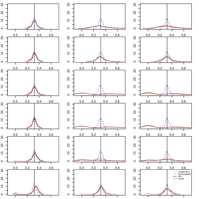
Figure 1: The (smoothed) empirical distribution of $\widehat{\mbox{CIF}}_{1}(2)$, estimated under the PCSH model with LASSO, for continuous covariates. The three columns correspond to $p=20$, 500, and 1000. The rows correspond to different ways of selecting $\lambda$, from top to bottom: 1) CV10, 2) CV+1SE, 3) minimum AIC, 4) minimum BIC, 5) elbow AIC and 6) elbow BIC. The true $\mbox{CIF}_{1}(2|z_{0})=0.32$.

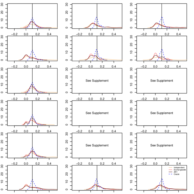
Figure 3: The (smoothed) empirical distribution of $\widehat{\mbox{CIF}}_{1}(2)$, estimated under the PCSH model with LASSO, for sparse binary covariates. The three columns correspond to $p=20$, 500, and 1000. The rows correspond to different ways of selecting $\lambda$, from top to bottom: 1) CV10, 2) CV+1SE, 3) minimum AIC, 4) minimum BIC, 5) elbow AIC and 6) elbow BIC. The true $\mbox{CIF}_{1}(2|z_{0})=0.11$.

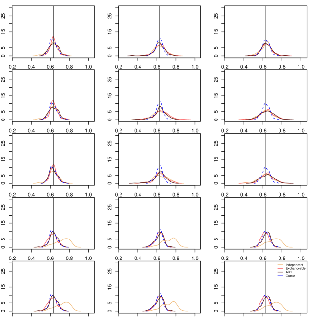
Figure 4: The (smoothed) empirical distribution of $\widehat{\mbox{CIF}}_{1}(2)$, estimated under the PSDH model with boosting, for continuous covariates. The three columns correspond to $p=20$, 500, and 1000. The rows correspond to different ways of selecting $\gamma$, from top to bottom: 1) CV10, 2) minimum AIC, 3) minimum BIC, 4) elbow AIC and 5) elbow BIC. The true $\mbox{CIF}_{1}(2|z_{0})=0.63$.

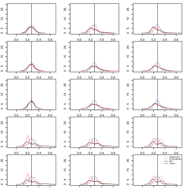
Figure 5: The (smoothed) empirical distribution of $\widehat{\mbox{CIF}}_{1}(2)$, estimated under the PSDH model with boosting, for balanced binary covariates. The three columns correspond to $p=20$, 500, and 1000. The rows correspond to different ways of selecting $\gamma$, from top to bottom: 1) CV10, 2) minimum AIC, 3) minimum BIC, 4) elbow AIC and 5) elbow BIC. The true $\mbox{CIF}_{1}(2|z_{0})=0.27$.

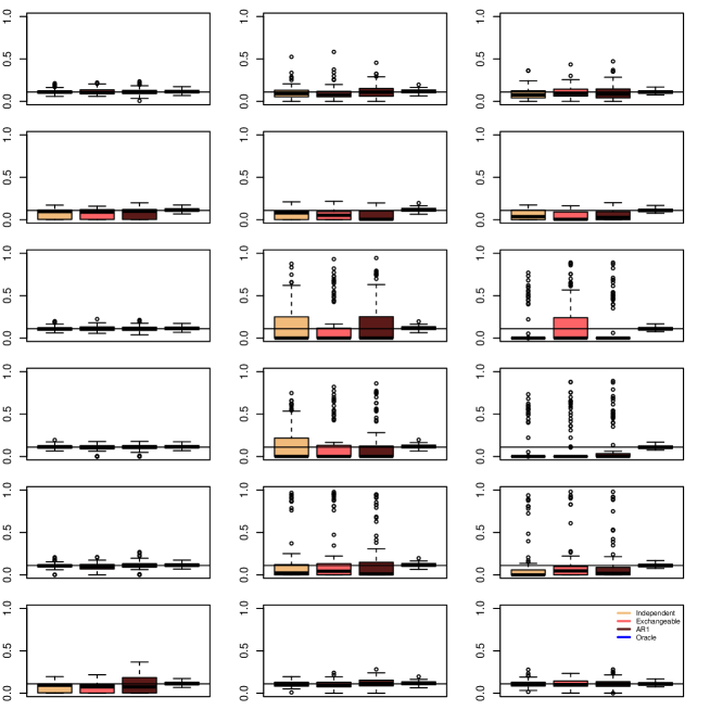
Figure 9: Boxplots of $\widehat{\mbox{CIF}}_{1}(2)$, estimated under the PCSH model with LASSO, for balanced binary covariates. The three columns correspond to $p=20$, 500, and 1000. The rows correspond to different ways of selecting $\lambda$, from top to botton: 1) CV10, 2) CV+1SE, 3) minimum AIC, 4) minimum BIC, 5) elbow AIC and 6) elbow BIC. The true $\mbox{CIF}_{1}(2|z_{0})=0.11$.

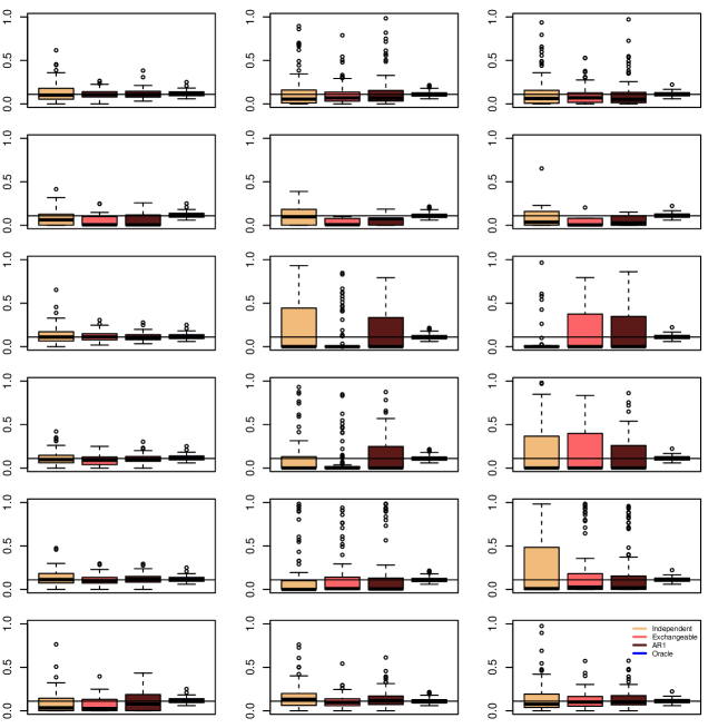
Figure 10: Boxplots of $\widehat{\mbox{CIF}}_{1}(2)$, estimated under the PCSH model with LASSO, for sparse binary covariates. The three columns correspond to $p=20$, 500, and 1000. The rows correspond to different ways of selecting $\lambda$, from top to botton: 1) CV10, 2) CV+1SE, 3) minimum AIC, 4) minimum BIC, 5) elbow AIC and 6) elbow BIC. The true $\mbox{CIF}_{1}(2|z_{0})=0.11$.

We evaluate the performance of prediction at a given covariate vector value $\bf{z}_{0}$. We set $\bm{z_{0}}=(0.5,\cdots,0.5)_{1\times p}$ for the continuous case; and for all the binary cases each element of $\bf{z}_{0}$ was independently drawn with a fixed seed from Bernoulli distribution with $p=0.5$. Figures 1 - 6 show the empirical distributions of the estimated $\mbox{CIF}_{1}(2)$ over the 100 simulation runs, where the vertical line marks the true $\mbox{CIF}_{1}(2)$; the empirical distributions were plotted using the R function ‘density()’. The PCSH model with LASSO was used to estimate $\mbox{CIF}_{1}(2)$ in Figures 1 - 10, and the PSDH model with boosting was used in Figures 4 - 6.

In the figures the blue dashed lines are for the oracle estimator, which fits the exact true active set $S(\beta)$. The oracle estimator varied extremely slightly when the three correlation structures for $Z$ were generated separately, which appeared to be due to Monte Carlo variation, and the one under the AR(1) structure is plotted here. It is seen that the distribution of the oracle estimator is more concentrated for the balanced binary covariates than for the sparse binary covariates, which reflects the ‘effective sample size’ that is reduced with the sparse binary covariates. The solid lines are the estimated $\mbox{CIF}_{1}(2)$ under each model after regularization using LASSO or boosting, with different colors representing different correlation structures of $Z$.

Under the PSDH model using LASSO to regularize, the performances were generally not satisfactory as compared to the oracle estimator. The worst performances were seen when using minimum AIC and BIC to choose the penalty parameter; some of these results were so extreme that ‘density()’ failed to work and these were instead shown in the Supplemental Materials using boxplots. Elbow BIC appeared to perform the best for continuous covariates, but not so for binary covariates even when $p=20$. CV10 had the best performance for binary covariates for $p=20$, but it too deteriorated for $p=500$ and 1000.

Under the PSDH model using boosting, in Figure 4 we see that for continuous covariates, the estimators performed reasonably well when CV10 or minimum AIC/BIC was used to choose the number of boosting steps; with CV10 the estimation was perhaps the best. The performance deteriorated with (balanced) binary covariates for $p=500$ and 1000. For the sparse binary covariates, even the oracle estimator had a very wide spread, with the performance of the regularized estimator under the independent structure the worst of all. We note that in Bühlmann [6] simulation studies (Table 1) the mean squared error for boosting with correlated design was also smaller than that with uncorrelated design, and their Figure 1 showed that boosting tended to select more covariates in the uncorrelated design than the correlated design.

The Supplemental Materials provide the results of variable selection; although this was not the main goal for our application and it was difficult to achieve good model consistency (i.e. selection), they help to explain the prediction accuracy. When the selection is extremely poor, for example a couple of hundred false positives, then the prediction results were very poor as well. Boosting had no more than five false positives in all cases.

5 SEER-Medicare linked data

We randomly split the SEER-Medicare dataset into approximate equal-sized training ($n=28,505$) and test ($n=28,506$) datasets. As a first step we excluded binary claim codes having less than 10 ones, with rest all being zero. We then used univariate screening to further reduce dimensionality, eliminate noise and increase the performance of subsequent variable selection methods [32].

5.1 PCSH model with LASSO

Univariate screening under the PCSH model with $p$-valued cutoff of 0.05 gave $p_{1}=2188$ and $p_{2}=1079$ claim codes for non-cancer and cancer mortality, respectively. For each type of mortality, we applied LASSO under the PCSH model described earlier on the training data with the above pre-screened claim codes plus the clinical and demographic variables. Based on the simulation results, CV10 was used to choose the penalty parameter. The final model contained 143 predictors for non-cancer mortality, and 9 predictors for cancer mortality. Since the regression coefficients from LASSO are biased, we refit the PCSH model with the selected predictors.

In order to evaluate the resulting prediction model on the test data, we first calculated the risk score $\hat{\beta}^{\prime}_{j}Z$ for each patient in the test data, $j=1,2$. For each mortality type $j$, we then divided the test set into 4 risk strata: low (L), median low (ML), median high (MH) and high (H) according to the quartiles. Combining the two types of mortalities, we formed a total of 16 strata for their predicted CIF. Using the average $Z$ values in each of the 16 strata, we plotted their predicted CIF’s for both cancer and non-cancer mortality (see Supplemental Materials). It was clear that instead of 16 groups, 5 distinct risk groups emerge for both cancer and non-cancer mortalities. We note that these are not the same 5 groups for the two types of mortality, and Table 1 provides the definition for each of them. It is perhaps not surprising to see that each mortality risk was most influenced by the corresponding cause-specific risk, and also secondarily by its competing risk.

In Figure 7 we plot the nonparametric CIF (solid lines) and its 95% confidence intervals (shaded) for each of the above 5 risk groups for each type of mortality. The clear separation of the 5 groups show the usefulness of the final PCSH model in classifying patients according to their different prognosis for both cancer and non-cancer mortalities. For comparison purposes we also plot the predicted CIF for each of the 5 risk groups. While the prediction is more accurate for the non-cancer CIF, the predicted cancer CIF seems less accurate especially for the high (H) risk group.

5.2 PSDH model with boosting

Univariate screening with $p$-value cutoff of 0.05 under the PSDH model initially gave $p_{1}=4634$ and $p_{2}=6088$ claim codes for non-cancer and cancer mortality, respectively. We further reduced the dimension by retaining only the top 2000 claim codes (ranked by $p$-value) for each type of mortality, to be comparable with the fitting of the PCSH model above, as well as for the boosting algorithm to be able to run on our Dell R630 computer (two Intel Xeon E5-2660 v3 2.6GHz, each processor with 10 cores (20 threads) for a total of 20 cores (40 threads), 128GB of DDR3). We applied boosting under the PSDH model to the training data with these claim codes plus the clinical and demographic variables. Although CV10 performed best in our simulation results, AIC was a close second especially for binary covariates and was less computationally intensive for this procedure where boosting itself was computationally intensive already. Therefore AIC was used to choose the optimal step. The final model contains $53$ predictors for non-cancer mortality, and $13$ predictors for cancer mortality. We refit the PSDH model with the selected predictors to obtain the unbiased estimator.

Similar to the abve, we calculated the risk score $\hat{\beta}^{\prime}_{j}Z$ for each patient in the test data, $j=1,2$. For each mortality type $j$, we divided the test set into 5 risk strata: low (L), median low (ML), median (M), median high (MH) and high (H) according to the quartiles. Again the classification was not the same 5 groups for the two types of morality. In Figure 8, we plot the nonparametric CIF (solid lines) and its 95% confidence intervals (shaded) for the above 5 risk groups for both non-cancer and cancer mortality. For comparison purposes we also plot the predicted CIF for each of the 5 risk groups. The prediction was still more accurate for the non-cancer CIF, and less so for cancer CIF especially for the high (H) risk group; however, compared to the PCSH model the separation of the 5 groups was less even, making the results perhaps less desirable for clinical use.

6 Discussion

The rapid accumulation of data across many fields, medicine in particular, has created unique challenges in statistics. The distinct issues with high dimensional data have come to be recognized recently, including for example, the rapid noise accumulation, the unrealistic independence assumption, and the necessity for novel robust data analysis methods [9]. While researchers work to meet these challenges, some of the methods proposed in the literature do not necessarily scale well to large data sets. In this paper, we considered the feasible implementations of statistical learning methods under the PCSH and PSDH models. We empirically studied their performance in variable selection and prediction through comprehensive simulations in both low- and high-dimensional settings with different covariate structures. By applying the methods to analyze a rich dataset with claim codes describing disease diagnoses, surgical procedures, hospitalization and outpatient activities, we created an individualized patient prediction tool aimed at helping prostate cancer patients and their physicians to better understand the prognosis for both cancer and other morbidities, which can in turn aid in clinical decision making.

For the linked SEER-Medicare data that we have considered, the PCSH model appears to outperform the PSDH model in terms of classifying patients into different risk groups for both cancer and non-cancer mortality. PCSH outperforming PSDH has not been previously observed; in the limited comparisons that we are aware of in the literature, the two seem to give somewhat comparable results [18]. While the PSDH model was proposed in order to associate the CIF due to one cause directly with the covariates without having to specifically model the other causes, the PCSH model might be more flexible precisely due to the fact that it allows different modeling of different causes in the denominator of the CIF. This is certainly worth future investigation. We also note that while the proportional hazards assumption is used in both models, there has been recent work considering other modeling approaches such as the additive hazards in the presence of competing risks [37].

Finally, we note that in the high-dimensional context methods developed for continuous data may behave differently for binary data especially if sparsity presents. In a recent paper Mukherjee et al. [25] showed that when a binary design matrix is sufficiently sparse, no signal can be detected irrespective of its strength. This finding echos the challenges that we have observed in our simulation studies.

Acknowledgement

This research was supported by a grant from the American Society of Clinical Oncology (ASCO), and was partially supported by the National Institutes of Health Clinical and Translational Science Award (CTSA) UL1TR001442.

Table 1: Five risk groups ($n$ and # events from test data) derived from the original 16 combinations of 4 non-cancer and 4 cancer cause-specific strata.

Risk Groups $$n$$ # events Cause-Specific

Non-cancer mortality: Non-cancer: Cancer:

L 7127 131 L L, ML, MH, H

ML 7126 280 ML L, ML, MH, H

M 7126 558 MH L, ML, MH, H

MH 3117 594 H L, ML, MH

H 4010 1022 H H

Cancer mortality: Non-cancer: Cancer:

L 7135 40 L, ML, MH, H L

ML 7118 51 L, ML, MH, H ML

M 7128 101 L, ML, MH, H MH

MH 3115 134 L, ML, MH H

H 4010 294 H H

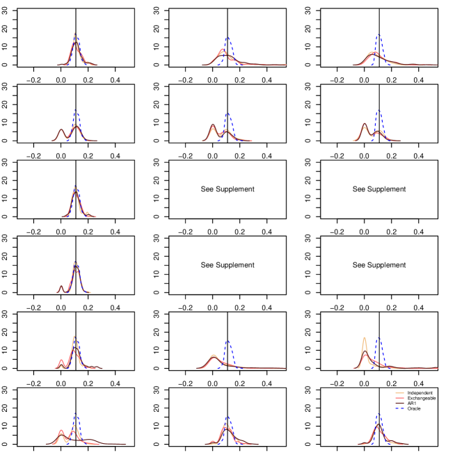
Figure 2: The (smoothed) empirical distribution of $\widehat{\mbox{CIF}}_{1}(2)$, estimated under the PCSH model with LASSO, for balanced binary covariates. The three columns correspond to $p=20$, 500, and 1000. The rows correspond to different ways of selecting $\lambda$, from top to bottom: 1) CV10, 2) CV+1SE, 3) minimum AIC, 4) minimum BIC, 5) elbow AIC and 6) elbow BIC. The true $\mbox{CIF}_{1}(2|z_{0})=0.11$.

Figure 6: The (smoothed) empirical distribution of $\widehat{\mbox{CIF}}_{1}(2)$, estimated under the PSDH model with boosting, for sparse binary covariates. The three columns correspond to $p=20$, 500, and 1000. The rows correspond to different ways of selecting $\gamma$, from top to bottom: 1) CV10, 2) minimum AIC, 3) minimum BIC, 4) elbow AIC and 5) elbow BIC. The true $\mbox{CIF}_{1}(2|z_{0})=0.27$.

Figure 7: Cumulative incidence functions for non-cancer (top) and cancer (bottom) mortalities, with classification and prediction based on the PCSH model. The shaded area is the 95% pointwise confidence intervals based on the nonparametric estimate.

Figure 8: Cumulative incidence functions for non-cancer (top) and cancer (bottom) mortalities, with classification and prediction based on the PSDH model. The shaded area is the 95% pointwise confidence intervals based on the nonparametric estimate.

7 Supplemental Materials

In the following tables, $|S(\hat{\beta})|$ is the size of the estimated active set, i.e. number of non-zero estimated regression coefficients. The median number of selected variables are reported, and in () are the median absolute deviation (MAD) of selection.

Table 2: The median (MAD) number of selected variables by LASSO under the PCSH model. The penalty parameter is chosen using CV10.

Cause 1 Continuous	$|S(\hat{\beta})|$	$\#$True Positives	$\#$False Positives
p=20
Independence	12(1)	5(0)	7(1)
Exchangeable	12(2)	5(0)	7(2)
AR1	12(1)	5(0)	7(1)
p=500
Independence	35(7)	5(0)	30(7)
Exchangeable	35(5)	5(0)	30(5)
AR1	37(6)	5(0)	32(6)
p=1000
Independence	41(8)	5(0)	36(8)
Exchangeable	44(7)	5(0)	39(7)
AR1	41(7.5)	5(0)	36(7.5)
Cause 1 Binary (balanced)	$|S(\hat{\beta})|$	$\#$True Positives	$\#$False Positives
p=20
Independence	11(2)	5(0)	6(2)
Exchangeable	12(2)	5(0)	7(2)
AR1	12(2)	5(0)	7(2)
p=500
Independence	22(6)	5(0)	17(6)
Exchangeable	27(6)	5(0)	22(6)
AR1	25(6)	5(0)	20(6)
p=1000
Independence	23(6)	5(0)	18(6)
Exchangeable	29(5)	5(0)	24(5)
AR1	27(8)	5(0)	22(8)
Cause 1 Binary (sparse)	$|S(\hat{\beta})|$	$\#$True Positives	$\#$False Positives
p=20
Independence	10(2)	5(0)	5(2)
Exchangeable	11(2)	5(0)	6(2)
AR1	11(2)	5(0)	6(2)
p=500
Independence	17.5(6.5)	4(1)	13(6)
Exchangeable	19.5(5.5)	4(0)	15(5)
AR1	20.5(5.5)	5(0)	15.5(5.5)
p=1000
Independence	17(6)	4(0.5)	13(6)
Exchangeable	20(6)	4(1)	16(6)
AR1	21.5(5.5)	5(0)	17.5(5.5)

Table 3: The median (MAD) number of selected variables by LASSO under the PCSH model. The penalty parameter is chosen using CV+1SE.

Cause 1 Continuous	$|S(\hat{\beta})|$	$\#$True Positives	$\#$False Positives
p=20
Independence	6(1)	5(0)	1(1)
Exchangeable	6(1)	5(0)	1(1)
AR1	6(1)	5(0)	1(1)
p=500
Independence	9(2)	5(0)	4(3)
Exchangeable	12(3)	5(0)	7(3)
AR1	10(3)	5(0)	5(3)
p=1000
Independence	9(3)	5(0)	4(3)
Exchangeable	13(4)	5(0)	8(4)
AR1	12(4)	5(0)	7(4)
Cause 1 Binary (balanced)	$|S(\hat{\beta})|$	$\#$True Positives	$\#$False Positives
p=20
Independence	5(0)	5(0)	0(0)
Exchangeable	5(1)	5(0)	0(0)
AR1	5(0)	5(0)	0(0)
p=500
Independence	5(1)	5(0)	1(1)
Exchangeable	6(1)	4(0)	2(1)
AR1	7(2)	5(0)	2(2)
p=1000
Independence	5(1)	5(0)	0(0)
Exchangeable	6(2)	4(0)	1(1)
AR1	6(1)	5(0)	1(1)
Cause 1 Binary (sparse)	$|S(\hat{\beta})|$	$\#$True Positives	$\#$False Positives
p=20
Independence	4(1)	4(1)	0(0)
Exchangeable	5(1)	4(1)	0(0)
AR1	5(1)	5(0)	0(0)
p=500
Independence	4(1)	4(1)	0(0)
Exchangeable	3(1)	3(1)	0(0)
AR1	4(1)	4(1)	0(0)
p=1000
Independence	3(1)	3(1)	0(0)
Exchangeable	3.5(1.5)	3(1)	0(0)
AR1	4(1)	4(1)	0(0)

Table 4: The median (MAD) number of selected variables by LASSO under the PCSH model. The penalty parameter is chosen using min AIC.

Cause 1 Continuous	$|S(\hat{\beta})|$	$\#$True Positives	$\#$False Positives
p=20
Independence	7(1)	5(0)	2(1)
Exchangeable	7(1)	5(0)	2(1)
AR1	7(1)	5(0)	2(1)
p=500
Independence	280(16.5)	5(0)	275(16.5)
Exchangeable	303.5(13)	5(0)	298.5(13)
AR1	295.5(11.5)	5(0)	290.5(11.5)
p=1000
Independence	260(15)	5(0)	255(15)
Exchangeable	292(16.5)	5(0)	287(16.5)
AR1	282(17)	5(0)	277(17)
Cause 1 Binary (balanced)	$|S(\hat{\beta})|$	$\#$True Positives	$\#$False Positives
p=20
Independence	7(1)	5(0)	2(1)
Exchangeable	7(1)	5(0)	2(1)
AR1	7(1)	5(0)	2(1)
p=500
Independence	364.5(16.5)	5(0)	359.5(16.5)
Exchangeable	372(17)	5(0)	367(17)
AR1	369(15)	5(0)	364(15)
p=1000
Independence	344(17.5)	5(0)	339.5(17.5)
Exchangeable	352(14.5)	5(0)	347(14.5)
AR1	362(16.5)	5(0)	357(16.5)
Cause 1 Binary (sparse)	$|S(\hat{\beta})|$	$\#$True Positives	$\#$False Positives
p=20
Independence	7(1)	5(0)	2.5(1.5)
Exchangeable	8(2)	5(0)	3(2)
AR1	7(1)	5(0)	2(1)
p=500
Independence	338(27.5)	5(0)	334(27)
Exchangeable	348(15.5)	5(0)	343(15)
AR1	352.5(15.5)	5(0)	347.5(15.5)
p=1000
Independence	329(27.5)	4.5(0.5)	324.5(27)
Exchangeable	336.5(19.5)	5(0)	331.5(19.5)
AR1	335.5(19.5)	5(0)	330.5(20)

Table 5: The median (MAD) number of selected variables by LASSO under the PCSH model. The penalty parameter is chosen using min BIC.

Cause 1 Continuous	$|S(\hat{\beta})|$	$\#$True Positives	$\#$False Positives
p=20
Independence	5(0)	5(0)	0(0)
Exchangeable	5(0)	5(0)	0(0)
AR1	5(0)	5(0)	0(0)
p=500
Independence	268(17)	5(0)	263(17)
Exchangeable	291(20)	5(0)	286(20)
AR1	286(17)	5(0)	281(17)
p=1000
Independence	253(12.5)	5(0)	248(12.5)
Exchangeable	268.5(17)	5(0)	263.5(17)
AR1	265(15)	5(0)	260(15)
Cause 1 Binary (balanced)	$|S(\hat{\beta})|$	$\#$True Positives	$\#$False Positives
p=20
Independence	5(0)	5(0)	0(0)
Exchangeable	5(0)	5(0)	0(0)
AR1	5(0)	5(0)	0(0)
p=500
Independence	354.5(17.5)	5(0)	349.5(17)
Exchangeable	359(23)	5(0)	354(23)
AR1	359(16)	5(0)	354(16)
p=1000
Independence	341(17)	5(0)	336(17)
Exchangeable	345.5(16)	5(0)	340.5(16)
AR1	354.5(18.5)	5(0)	349.5(18.5)
Cause 1 Binary (sparse)	$|S(\hat{\beta})|$	$\#$True Positives	$\#$False Positives
p=20
Independence	5(1)	4(0)	0(0)
Exchangeable	5(1)	4(0)	0(0)
AR1	5(0)	5(0)	0(0)
p=500
Independence	319(41)	5(0)	315(40.5)
Exchangeable	345(18)	5(0)	340(18)
AR1	343(23)	5(0)	338(23)
p=1000
Independence	321.5(26)	5(0)	317(26)
Exchangeable	323(24.5)	5(0)	318(24)
AR1	322.5(24)	5(0)	318(24)

Table 6: The median (MAD) number of selected variables by LASSO under the PCSH model. The penalty parameter is chosen using elbow AIC.

Cause 1 Continuous	$|S(\hat{\beta})|$	$\#$True Positives	$\#$False Positives
p=20
Independence	5.5(0.5)	5(0)	0.5(0.5)
Exchangeable	5(1)	5(0)	0(0)
AR1	5(1)	5(0)	0(0)
p=500
Independence	225(21)	5(0)	220(21)
Exchangeable	27.5(18.5)	5(0)	22.5(18.5)
AR1	200(51)	5(0)	195(51)
p=1000
Independence	162.5(72)	5(0)	157.5(72)
Exchangeable	31.5(22)	5(0)	26.5(22)
AR1	61(49)	5(0)	56(49)
Cause 1 Binary (balanced)	$|S(\hat{\beta})|$	$\#$True Positives	$\#$False Positives
p=20
Independence	6(1)	5(0)	1(1)
Exchangeable	5(1)	5(0)	0(0)
AR1	5(1)	5(0)	0(0)
p=500
Independence	271.5(41)	5(0)	266.5(41)
Exchangeable	171.5(127.5)	5(0)	166.5(127.5)
AR1	277(40)	5(0)	272(40)
p=1000
Independence	271(26)	5(0)	266(26)
Exchangeable	70.5(60)	5(0)	65.5(59.5)
AR1	247(68)	5(0)	242(68)
Cause 1 Binary (sparse)	$|S(\hat{\beta})|$	$\#$True Positives	$\#$False Positives
p=20
Independence	5(1)	4(1)	1(1)
Exchangeable	5(1)	5(0)	1(1)
AR1	6(1)	5(0)	1(1)
p=500
Independence	222.5(77.5)	5(0)	217.5(77)
Exchangeable	105.5(79.5)	5(0)	100.5(78.5)
AR1	256(40)	5(0)	251(40)
p=1000
Independence	114.5(75.5)	4(1)	110.5(75.5)
Exchangeable	101(68.5)	5(0)	96(68)
AR1	210(73)	5(0)	205(73)

Table 7: The median (MAD) number of selected variables by LASSO under the PCSH model. The penalty parameter is chosen using elbow BIC.

Cause 1 Continuous	$|S(\hat{\beta})|$	$\#$True Positives	$\#$False Positives
p=20
Independence	4(0)	4(0)	0(0)
Exchangeable	4(0)	4(0)	0(0)
AR1	4(0)	4(0)	0(0)
p=500
Independence	5(1)	5(0)	0(0)
Exchangeable	5(1)	4(1)	0(0)
AR1	5(1)	5(0)	0(0)
p=1000
Independence	6.5(1.5)	5(0)	1.5(1.5)
Exchangeable	5(1)	4(1)	0(0)
AR1	6(1)	5(0)	1(1)
Cause 1 Binary (balanced)	$|S(\hat{\beta})|$	$\#$True Positives	$\#$False Positives
p=20
Independence	4(0)	4(0)	0(0)
Exchangeable	4(0)	4(0)	0(0)
AR1	4(0)	4(0)	0(0)
p=500
Independence	6(1)	5(0)	1(1)
Exchangeable	5(1)	4(0)	1(1)
AR1	6(1)	5(0)	1(1)
p=1000
Independence	8(2)	5(0)	3(2)
Exchangeable	6(2)	4(0)	2(1)
AR1	7(2)	5(0)	2(1)
Cause 1 Binary (sparse)	$|S(\hat{\beta})|$	$\#$True Positives	$\#$False Positives
p=20
Independence	3(1)	3(1)	0(0)
Exchangeable	3(1)	3(0.5)	0(0)
AR1	4(1)	4(0.5)	0(0)
p=500
Independence	6(2)	4(1)	2(2)
Exchangeable	5(1)	4(0)	2(1)
AR1	6(1)	4(1)	2(1)
p=1000
Independence	7(2)	4(1)	3(2)
Exchangeable	7(2)	4(1)	3(2)
AR1	7(2)	4(0)	3(2)

Table 8: The median (MAD) number of selected variables by LASSO under the PSDH model. The number of steps is chosen using CV10.

Cause 1 Continuous	$|S(\hat{\beta})|$	$\#$True Positives	$\#$False Positives
p=20
Independence	7(2)	5(0)	2(2)
Exchangeable	10(3)	5(0)	5(3)
AR1	9(2)	5(0)	4(2)
p=500
Independence	5(0)	5(0)	0(0)
Exchangeable	6(1)	5(0)	1(1)
AR1	6(1)	5(0)	1(1)
p=1000
Independence	5(0)	5(0)	0(0)
Exchangeable	5(0)	5(0)	0(0)
AR1	5(0)	5(0)	0(0)
Cause 1 Binary (balanced)	$|S(\hat{\beta})|$	$\#$True Positives	$\#$False Positives
p=20
Independence	6(1)	5(0)	1(1)
Exchangeable	7(2)	5(0)	2(2)
AR1	6(1)	5(0)	1(1)
p=500
Independence	5(1)	5(0)	0(0)
Exchangeable	4(1)	4(0)	0(0)
AR1	4.5(0.5)	4(0)	0(0)
p=1000
Independence	5(1)	4(1)	0(0)
Exchangeable	4(0)	4(0)	0(0)
AR1	4(0)	4(0)	0(0)
Cause 1 Binary (sparse)	$|S(\hat{\beta})|$	$\#$True Positives	$\#$False Positives
p=20
Independence	5(1)	4(1)	0(0)
Exchangeable	6(1)	5(0)	1(1)
AR1	5(1)	5(0)	0(0)
p=500
Independence	3(1)	2(1)	0(0)
Exchangeable	3(0)	3(0)	0(0)
AR1	3(0)	3(0)	0(0)
p=1000
Independence	2(1)	2(1)	0(0)
Exchangeable	3(0)	3(0)	0(0)
AR1	3(0)	3(0)	0(0)

Table 9: The median (MAD) number of selected variables by LASSO under the PSDH model. The number of steps is chosen using min AIC.

Cause 1 Continuous	$|S(\hat{\beta})|$	$\#$True Positives	$\#$False Positives
p=20
Independence	7(1)	5(0)	2(1)
Exchangeable	7(1)	5(0)	2(1)
AR1	7(1)	5(0)	2(1)
p=500
Independence	7(1)	5(0)	2(1)
Exchangeable	8(1)	5(0)	3(1)
AR1	7.5(1.5)	5(0)	2.5(1.5)
p=1000
Independence	7(1)	5(0)	2(1)
Exchangeable	7(1)	5(0)	2(1)
AR1	7(1)	5(0)	2(1)
Cause 1 Binary (balanced)	$|S(\hat{\beta})|$	$\#$True Positives	$\#$False Positives
p=20
Independence	7(1)	5(0)	2(1)
Exchangeable	7(1)	5(0)	2.5(1.5)
AR1	7(1)	5(0)	2(1)
p=500
Independence	7(1)	5(0)	2(0)
Exchangeable	7(1)	5(0)	2(1)
AR1	7(0)	5(0)	2(0)
p=1000
Independence	7(1)	5(0)	2(1)
Exchangeable	6(1)	5(0)	2(1)
AR1	7(0)	5(0)	2(0)
Cause 1 Binary (sparse)	$|S(\hat{\beta})|$	$\#$True Positives	$\#$False Positives
p=20
Independence	6(1)	5(0)	2(1)
Exchangeable	7(1)	5(0)	2(1)
AR1	6(1)	5(0)	2(1)
p=500
Independence	5(1)	4(1)	1(1)
Exchangeable	6(1)	4(0)	2(0.5)
AR1	6(0)	5(0)	2(1)
p=1000
Independence	4(1)	3(1)	1(1)
Exchangeable	6(0)	4(0)	2(0)
AR1	6(0)	4(0)	2(1)

Table 10: The median (MAD) number of selected variables by LASSO under the PSDH model. The number of steps is chosen using min BIC.

Cause 1 Continuous	$|S(\hat{\beta})|$	$\#$True Positives	$\#$False Positives
p=20
Independence	5(0)	5(0)	0(0)
Exchangeable	5(0)	5(0)	0(0)
AR1	5(0)	5(0)	0(0)
p=500
Independence	7(1)	5(0)	2(1)
Exchangeable	7(1)	5(0)	2(1)
AR1	7(1)	5(0)	2(1)
p=1000
Independence	7(1)	5(0)	2(1)
Exchangeable	7(1)	5(0)	2(1)
AR1	7(1)	5(0)	2(1)
Cause 1 Binary (balanced)	$|S(\hat{\beta})|$	$\#$True Positives	$\#$False Positives
p=20
Independence	5(0)	5(0)	0(0)
Exchangeable	5(0)	5(0)	0(0)
AR1	5(0)	5(0)	0(0)
p=500
Independence	7(1)	5(0)	2(0.5)
Exchangeable	6(1)	5(0)	2(1)
AR1	7(0.5)	5(0)	2(0)
p=1000
Independence	7(1)	5(0)	2(1)
Exchangeable	6(1)	5(0)	2(1)
AR1	7(0)	5(0)	2(0)
Cause 1 Binary (sparse)	$|S(\hat{\beta})|$	$\#$True Positives	$\#$False Positives
p=20
Independence	4(1)	4(1)	0(0)
Exchangeable	5(0)	5(0)	0(0)
AR1	5(0)	5(0)	0(0)
p=500
Independence.	4.5(0.5)	4(1)	1(1)
Exchangeable.	6(1)	4(0)	2(1)
AR1	6(0.5)	4.5(0.5)	2(1)
p=1000
Independence	4(1)	3(1)	1(1)
Exchangeable	6(0)	4(0)	2(0)
AR1	6(0)	4(0)	2(1)

Table 11: The median (MAD) number of selected variables by LASSO under the PSDH model. The number of steps is chosen using elbow AIC.

Cause 1 Continuous	$|S(\hat{\beta})|$	$\#$True Positives	$\#$False Positives
p=20
Independence	3(0)	3(0)	0(0)
Exchangeable	4(1)	4(1)	0(0)
AR1	4.5(0.5)	4.5(0.5)	0(0)
p=500
Independence	3(0)	3(0)	0(0)
Exchangeable	4(0)	4(0)	0(0)
AR1	4(1)	4(1)	0(0)
p=1000
Independence	4(1)	4(1)	0(0)
Exchangeable	4(1)	4(1)	0(0)
AR1	4.5(0.5)	4.5(0.5)	0(0)
Cause 1 Binary (balanced)	$|S(\hat{\beta})|$	$\#$True Positives	$\#$False Positives
p=20
Independence	3(0)	3(0)	0(0)
Exchangeable	3.5(0.5)	3.5(0.5)	0(0)
AR1	4(0)	4(0)	0(0)
p=500
Independence	3(0)	3(0)	0(0)
Exchangeable	3(1)	3(1)	0(0)
AR1	4(0)	4(0)	0(0)
p=1000
Independence	3(0)	3(0)	0(0)
Exchangeable	3(1)	3(1)	0(0)
AR1	4(0)	4(0)	0(0)
Cause 1 Binary (sparse)	$|S(\hat{\beta})|$	$\#$True Positives	$\#$False Positives
p=20
Independence	3(1)	3(1)	0(0)
Exchangeable	3(1)	3(1)	0(0)
AR1	4(0.5)	4(0.5)	0(0)
p=500
Independence	3(1)	3(1)	0(0)
Exchangeable	3(1)	3(1)	0(0)
AR1	4(0.5)	4(0.5)	0(0)
p=1000
Independence	2(1)	2(1)	0(0)
Exchangeable	3(1)	3(1)	0(0)
AR1	4(0)	4(0)	0(0)

Table 12: The median (MAD) number of selected variables by LASSO under the PSDH model. The number of steps is chosen using elbow BIC.

Cause 1 Continuous	$|S(\hat{\beta})|$	$\#$True Positives	$\#$False Positives
p=20
Independence	3(0)	3(0)	0(0)
Exchangeable	4(1)	4(1)	0(0)
AR1	4.5(0.5)	4.5(0.5)	0(0)
p=500
Independence	3(0)	3(0)	0(0)
Exchangeable	4(0)	4(0)	0(0)
AR1	4(1)	4(1)	0(0)
p=1000
Independence	4(1)	4(1)	0(0)
Exchangeable	4(1)	4(1)	0(0)
AR1	4.5(0.5)	4.5(0.5)	0(0)
Cause 1 Binary (balanced)	$|S(\hat{\beta})|$	$\#$True Positives	$\#$False Positives
p=20
Independence	3(0)	3(0)	0(0)
Exchangeable	3.5(0.5)	3.5(0.5)	0(0)
AR1	4(0)	4(0)	0(0)
p=500
Independence	3(0)	3(0)	0(0)
Exchangeable	3(1)	3(1)	0(0)
AR1	4(0)	4(0)	0(0)
p=1000
Independence	3(0)	3(0)	0(0)
Exchangeable	3(1)	3(1)	0(0)
AR1	4(0)	4(0)	0(0)
Cause 1 Binary (sparse)	$|S(\hat{\beta})|$	$\#$True Positives	$\#$False Positives
p=20
Independence	3(1)	3(1)	0(0)
Exchangeable	3(1)	3(1)	0(0)
AR1	4(0.5)	4(0.5)	0(0)
p=500
Independence	3(1)	3(1)	0(0)
Exchangeable	3(1)	3(1)	0(0)
AR1	4(0.5)	4(0.5)	0(0)
p=1000
Independence	2(1)	2(1)	0(0)
Exchangeable	3(1)	3(1)	0(0)
AR1	4(0)	4(0)	0(0)

The following two figures correspond to the main paper Figure 2 and 3, where ‘density()’ failed in some cases to properly depict the empirical distribution of $\widehat{\mbox{CIF}}_{1}(2)$.

Figure 11: Predicted 16-group cumulative incidence functions for non-cancer and cancer mortality, based on 4 non-cancer and 4 cancer strata under the PCSH model.

References

- [1] Jan Beyersmann, Markus Dettenkofer, Hartmut Bertz, and Martin Schumacher. A competing risks analysis of bloodstream infection after stem-cell transplantation using subdistribution hazards and cause-specific hazards. Statistics in medicine, 26(30):5360–5369, 2007.
- [2] Jan Beyersmann, Aurelien Latouche, Anika Buchholz, and Martin Schumacher. Simulating competing risks data in survival analysis. Statistics in medicine, 28(6):956–971, 2009.
- [3] Harald Binder, Arthur Allignol, Martin Schumacher, and Jan Beyersmann. Boosting for high-dimensional time-to-event data with competing risks. Bioinformatics, 25(7):890–896, 2009.
- [4] Jelena Bradic, Jianqing Fan, and Jiancheng Jiang. Regularization for Cox’s proportional hazards model with np-dimensionality. Annals of statistics, 39(6):3092, 2011.
- [5] Norman Breslow. Covariance analysis of censored survival data. Biometrics, pages 89–99, 1974.
- [6] Peter Bühlmann. Boosting for high-dimensional linear models. The Annals of Statistics, 34(2):559–583, 2006.
- [7] Peter Bühlmann and S van de Geer. Statistics for high-dimensional data: methods, theory and applications. Springer, 2011.
- [8] SC Cheng, Jason P Fine, and LJ Wei. Prediction of cumulative incidence function under the proportional hazards model. Biometrics, pages 219–228, 1998.
- [9] Jianqing Fan, Fang Han, and Han Liu. Challenges of big data analysis. National Science Review, 1(2):293–314, 2014.
- [10] Jianqing Fan and Runze Li. Variable selection via nonconcave penalized likelihood and its oracle properties. Journal of the American Statistical Association, 96(456):1348–1360, 2001.
- [11] Jason P Fine and Robert J Gray. A proportional hazards model for the subdistribution of a competing risk. Journal of the American statistical association, 94(446):496–509, 1999.
- [12] Thomas R Fleming and David P Harrington. Counting processes and survival analysis, volume 169. John Wiley & Sons, 2011.
- [13] Yoav Freund and Robert E Schapire. A desicion-theoretic generalization of on-line learning and an application to boosting. Journal of Computer and System Sciences, 55:119–139, 1997.
- [14] Jerome H Friedman. Greedy function approximation: a gradient boosting machine. Annals of statistics, 29(5):1189–1232, 2001.
- [15] Z Fu, C R Parikh, and B Zhou. Penalized variable selection in competing risks regression. Lifetime Data Analysis, pages doi:10.1007/s10985–016–9362–3, 2016.
- [16] Jan Gertheiss and Gerhard Tutz. Sparse modeling of categorial explanatory variables. The Annals of Applied Statistics, 4(4):2150–2180, 2010.
- [17] R B Geskus. Cause-specific cumulative incidence estimation and the Fine-Gray model under both left truncation and right censoring. Biometrics, 67(1):39–49, 2011.
- [18] R B Geskus. Data analysis with competing risks and intermediate states. Taylor & Francis Group, LLC. Boca Raton, FL., 2016.
- [19] Robert J Gray. A class of K-sample tests for comparing the cumulative incidence of a competing risk. The Annals of statistics, 16(3):1141–1154, 1988.
- [20] Torsten Hothorn, Peter Bühlmann, Sandrine Dudoit, Annette Molinaro, and Mark J Van Der Laan. Survival ensembles. Biostatistics, 7(3):355–373, 2006.
- [21] Jiayi Hou and Ronghui Xu. CompetingRisk: The Semi-Parametric Cumulative Incidence Function, 2017. R package version 1.0.
- [22] John D Kalbfleisch and Ross L Prentice. The statistical analysis of failure time data, volume 360. John Wiley & Sons, 2011.
- [23] Stéphane G Mallat and Zhifeng Zhang. Matching pursuits with time-frequency dictionaries. IEEE Transactions on Signal Processing, 41(12):3397–3415, 1993.
- [24] Nicolai Meinshausen and Peter Bühlmann. High-dimensional graphs and variable selection with the lasso. Annals of Statistics, pages 1436–1462, 2006.
- [25] Rajarshi Mukherjee, Natesh S Pillai, and Xihong Lin. Hypothesis testing for high-dimensional sparse binary regression. Annals of Statistics, 43(1):352, 2015.
- [26] Ian Thompson, James Brantley Thrasher, Gunnar Aus, Arthur L Burnett, Edith D Canby-Hagino, Michael S Cookson, Anthony V D’Amico, Roger R Dmochowski, David T Eton, Jeffrey D Forman, et al. Guideline for the management of clinically localized prostate cancer: 2007 update. The Journal of urology, 177(6):2106–2131, 2007.
- [27] Robert Tibshirani. Regression shrinkage and selection via the Lasso. Journal of the Royal Statistical Society. Series B (Methodological), pages 267–288, 1996.
- [28] Robert Tibshirani. The lasso method for variable selection in the Cox model. Statistics in medicine, 16(4):385–395, 1997.
- [29] Robert Tibshirani, G Walther, and T Hastie. estimating the number of clusters in a dataset via the gap statistic. Journal of the Royal Statistical Society, Series B, 63(2):411–423, 2001.
- [30] Pierre JM Verweij and Hans C Van Houwelingen. Cross-validation in survival analysis. Statistics in Medicine, 12(24):2305–2314, 1993.
- [31] C T Volinsky and A E Raftery. Bayesian information criterion for censored survival models. Biometrics, 56:256–262, 2000.
- [32] Larry Wasserman and Kathryn Roeder. High dimensional variable selection. Annals of Statistics, 37(5A):2178–2201, 2009.
- [33] R. Xu, F. Vaida, and D. P. Harrington. Using profile likelihood for semiparametric model selection with application to proportional hazards mixed models. Statistica Sinica, 19:819–842, 2009.
- [34] Ming Yuan and Yi Lin. Model selection and estimation in regression with grouped variables. Journal of the Royal Statistical Society: Series B (Statistical Methodology), 68(1):49–67, 2006.
- [35] Hao Helen Zhang and Wenbin Lu. Adaptive lasso for Cox’s proportional hazards model. Biometrika, 94(3):691–703, 2007.
- [36] Peng Zhao and Bin Yu. On model selection consistency of lasso. Journal of Machine Learning Research, 7(Nov):2541–2563, 2006.
- [37] C Zheng, R Dai, P N Hari, and M-J Zhang. Instrumental variable with competing risk model. Statistics in Medicine, 36:1240–1255, 2017.
- [38] Hui Zou. The adaptive lasso and its oracle properties. Journal of the American Statistical Association, 101(476):1418–1429, 2006.