The Velocity Dispersion Function for Quiescent Galaxies in the Local Universe

Abstract

We investigate the distribution of central velocity dispersions for quiescent galaxies in the SDSS at $0.03\leq z\leq 0.10$. To construct the field velocity dispersion function (VDF), we construct a velocity dispersion complete sample of quiescent galaxies with $D_{n}4000>1.5$. The sample consists of galaxies with central velocity dispersion larger than the velocity dispersion completeness limit of the SDSS survey. Our VDF measurement is consistent with previous field VDFs for $\sigma>200~{}\rm km~{}s^{-1}$. In contrast with previous results, the VDF does not decline significantly for $\sigma<200~{}\rm km~{}s^{-1}$. The field and the similarly constructed cluster VDFs are remarkably flat at low velocity dispersion ($\sigma<250~{}\rm km~{}s^{-1}$). The cluster VDF exceeds the field for $\sigma>250~{}\rm km~{}s^{-1}$ providing a measure of the relatively larger number of massive subhalos in clusters. The VDF is a probe of the dark matter halo distribution because the measured central velocity dispersion may be directly proportional to the dark matter velocity dispersion. Thus the VDF provides a potentially powerful test of simulations for models of structure formation.

1. INTRODUCTION

The stellar velocity dispersion of galaxy is a fundamental observable that is correlated with other basic properties of galaxies including luminosity ($L-\sigma^{4}$ relation, Faber & Jackson, 1976) and size and surface brightness (the fundamental plane, Djorgovski & Davis, 1987; Dressler et al., 1987). The velocity dispersion, often measured within the central region of a galaxy, reflects the dynamics of its stellar population. The velocity dispersion for a quiescent galaxy is particularly interesting because it is related to the mass of the galaxy through the virial theorem (e.g. Faber & Jackson, 1976; Bezanson et al., 2011; Zahid & Geller, 2017).

The central velocity dispersion (velocity dispersion hereafter) is a robust spectroscopic measure insensitive to the photometric biases that impact measurements of other fundamental observables including luminosity and stellar mass (Bernardi et al., 2013). Thus, the velocity dispersion of the stellar population may be the best observable connect galaxies directly to their dark matter (DM) halos (Wake et al., 2012a, b; Bogdán & Goulding, 2015; Zahid et al., 2016). Zahid et al. (2016) show that there is a scaling between central velocity dispersion and stellar mass, $\sigma\varpropto M_{*}^{0.3}$. This scaling is consistent with the scaling between the velocity dispersion of DM halo and total halo mass, $\sigma_{DM}\varpropto M_{halo}^{0.28-0.33}$, measured from N-body simulations (Evrard et al., 2008; Posti et al., 2014). Based on the consistency of these scaling relations, Zahid et al. (2016) suggest that the measured central velocity dispersion is proportional to the velocity dispersion of DM halo. Several studies also show that the central stellar velocity dispersion of elliptical galaxies is essentially identical to the velocity dispersion estimated from the best-fit strong lensing models (e.g. Treu et al., 2006; Grillo et al., 2008; Auger et al., 2010). These strong lensing studies underscore the fundamental importance of the central velocity dispersions.

The velocity dispersion distribution, i.e., the velocity dispersion function (VDF hereafter), has been measured for general field galaxies based on the SDSS and BOSS galaxy surveys (Sheth et al., 2003; Mitchell et al., 2005; Choi et al., 2007; Bernardi et al., 2010; Montero-Dorta et al., 2017). These VDFs measured from the general galaxy population, which we refer to as field VDFs, have similar shapes at $\sigma>150~{}\rm km~{}s^{-1}$, but they differ substantially for $\sigma\leq 150~{}\rm km~{}s^{-1}$. Choi et al. (2007) attribute the discrepancy at the low velocity dispersion to differences in sample selection including the definition of quiescent galaxies. Comparison among these previous field VDFs suggests that sample selection is critical for determining the shape of the VDF.

VDFs of cluster galaxies also differ from the field VDFs (Munari et al., 2016; Sohn et al., 2017). Sohn et al. (2017) compare VDFs for the massive clusters Coma and A2029 with previous field VDFs. They show that the cluster VDFs significantly exceed the field VDFs at high ($\sigma>250~{}\rm km~{}s^{-1}$) and low ($\sigma<150~{}\rm km~{}s^{-1}$) velocity dispersion. They suggest that the relatively large abundance of massive cluster members with large velocity dispersion results in the excess for $\sigma>250~{}\rm km~{}s^{-1}$. The cluster sample of Sohn et al. (2017) differs from the previous field samples in the definition of quiescent galaxies and in the corrections to velocity dispersion. These differences may be responsible for the difference in the VDFs for $\sigma<150~{}\rm km~{}s^{-1}$. Here, we explore this discrepancy by selecting a field sample in a way that is essentially identical to the cluster sample.

Statistical analyses of galaxy properties like the VDF require samples that cover the complete distribution of the galaxy properties. For example, luminosity functions are only complete to the absolute magnitude limit of a volume limited sample. Likewise, stellar mass functions can be measured from a sample that completely surveys the range of stellar masses (Fontana et al., 2006; Pérez-González et al., 2008; Pozzetti et al., 2010; Weigel et al., 2016). Stellar mass complete samples have been based on empirically derived stellar mass completeness limits as a function of redshift (Pozzetti et al., 2010; Weigel et al., 2016). A robust VDF measurement also requires a sample that includes the complete range of the velocity dispersions at each absolute magnitude. Here we derive a robust measurement of the VDF by empirically determining the velocity dispersion completeness limit.

We examine the VDF for the general field based on the extensive SDSS spectroscopic survey data. In contrast with previous approaches, we construct a velocity dispersion complete sample from the SDSS survey. To compare our result directly with the cluster VDFs of Sohn et al. (2017), we select the field sample according to the prescription of Sohn et al. (2017). Comparison between the field and cluster VDFs offers potential constraints on structure formation models and may be particularly interesting for understanding the formation and evolution of galaxies in the cluster environment.

We describe the data in Section 2. We explain the construction of the velocity dispersion complete sample in Section 3. Section 4 describes the method we use to measure the VDF. We discuss the results in Section 5 and we conclude in Section 6. Throughout the paper, we adopt the standard $\Lambda$CDM cosmology of $H_{0}=70~{}\rm km~{}s^{-1}~{}Mpc^{-1}$, $\Omega_{m}=0.3$, and $\Omega_{\Lambda}=0.7$.

2. DATA

Our primary goals are 1) measuring the velocity dispersion distribution function for field galaxies from a complete sample of galaxy central velocity dispersions and 2) comparing the VDF with previous results for the field and clusters. Here, we describe the galaxy sample, the photometric data (Section 2.1) and the spectroscopic properties of the sample including the galaxy central velocity dispersion (velocity dispersion hereafter, Section 2.2) and the $D_{n}4000$ index (Section 2.3). For a fair comparison with the cluster sample, we determine the field galaxy sample in the same way we define the cluster population. We construct a dataset that includes the entire range of galaxy velocity dispersions at every K-corrected absolute magnitude (see Section 3). We call this dataset the velocity dispersion complete sample.

2.1. Photometric Data

We use the Main Galaxy Sample (Strauss et al., 2002) from the Sloan Digital Sky Survey (SDSS) Data Release 12 (Alam et al., 2015). The Main Galaxy Sample is a magnitude limited sample with $r_{\rm petro}<17.77$ and $z\lesssim 0.3$. The SDSS spectroscopic survey is $\sim 95\%$ complete. The spectra cover $3500-9000$ Å with a resolution of $R\sim 1500$ at 5000 Å. We use galaxies in the Main Galaxy Sample in the redshift range $0.01<z<0.10$. We apply the lower redshift limit to minimize the influence of peculiar motions.

We K-correct the r-band magnitude to derive luminosities of galaxies over a wide redshift range. We use the $z=0$ K-correction from the NYU Value Added Galaxy Catalog (Blanton et al., 2005). We correct the SDSS spectroscopic limit by applying a median K-correction as a function of redshift (see Figure 2 in Zahid & Geller, 2017). We refer to the K-corrected r-band absolute magnitude as $M_{r}$.

2.2. Velocity dispersion

We adopt the velocity dispersions measured by the Portsmouth reduction (Thomas et al., 2013). The Portsmouth velocity dispersions are measured from SDSS spectra using the Penalized Pixel-Fitting (pPXF) code (Cappellari & Emsellem, 2004). In this procedure, stellar population templates from Maraston & Strömbäck (2011) which is based on the MILES stellar library (Sánchez-Blázquez et al., 2006) are converted to SDSS resolution. By comparing the SDSS spectra and the templates, the best-fit velocity dispersion is derived for each galaxy.

We compare the Portsmouth velocity dispersions for galaxies in the field sample with velocity dispersions for cluster members from the same reduction (Section 5.3). Sohn et al. (2017) measure the velocity dispersion function for Coma using velocity dispersion based on the Portsmouth reduction and for Abell 2029 based on the velocity dispersion from observations with Hectospec on MMT (Fabricant et al., 2005), respectively. Because the fiber sizes of SDSS spectrograph and Hectospec differ, an aperture correction is necessary. Following Sohn et al. (2017), the aperture correction is

$$(\sigma_{\rm SDSS}/\sigma_{\rm Hectospec})=(R_{\rm SDSS}/R_{\rm Hectospec})^{-0.054\pm 0.005},$$ (1)

where $R_{\rm SDSS}=1.\arcsec 5$ and $R_{\rm Hectospec}=0.\arcsec 75$. This aperture correction is consistent with previous determinations (Cappellari & Emsellem, 2004; Zahid et al., 2016).

Coma ($z=0.023$) and A2029 ($z=0.078$) are at different redshifts. Thus, the fibers cover different physical apertures for the galaxies in the two clusters. Using equation 1, Sohn et al. (2017) correct the velocity dispersion to a fiducial aperture of 3 kpc.

To compare the field and cluster VDFs directly, we use a velocity dispersion within 3 kpc following Sohn et al. (2017). We apply the aperture correction to the Portsmouth velocity dispersion for the galaxies in the magnitude limited sample. The aperture correction is small ($\sim 0.01$ dex) and does not significantly impact our results. Hereafter, we refer to this velocity dispersion within a 3 kpc aperture as $\sigma$.

2.3. $D_{n}4000$

We use $D_{n}4000$ from the MPA/JHU Catalog to identify quiescent galaxies. $D_{n}4000$ is a spectroscopic measure of the amplitude of the 4000 Å break. Balogh et al. (1999) define $D_{n}4000$ as the ratio of the flux in the $4000-4100$ Å and $3850-3950$ Å bands (Balogh et al., 1999).

$D_{n}4000$ is a stellar population age indicator (Kauffmann et al., 2003; Geller et al., 2014) showing a bimodal distribution (Kauffmann et al., 2003). Thus, the index is often used to segregate star-forming and quiescent galaxies (Kauffmann et al., 2003; Mignoli et al., 2005; Vergani et al., 2008; Woods et al., 2010; Zahid et al., 2016). $D_{n}4000$ is a powerful tool because it can be measured at high signal to noise directly from the spectra. This index is insensitive to photometric issues including seeing, crowding of galaxies and reddening. $D_{n}4000$ is also a redshift independent index. Thus, it is a relatively clean basis for construction of VDFs in a wide range of environments and at a wide range of redshifts.

We identify quiescent galaxies as objects with $D_{n}4000>1.5$. The $D_{n}4000$ selection is the same as the one used by Sohn et al. (2017) who examine VDFs for quiescent galaxies in Coma and A2029. Sohn et al. (2017) use $D_{n}4000$ for A2029 members from Hectospec observations. The $D_{n}4000$ measurements from SDSS and Hectospec for the same objects are within $\sim 5\%$, a difference that does not affect our analysis (Fabricant et al., 2013). We note that our results are insensitive to the $D_{n}4000$ selection. If we select quiescent galaxies with $D_{n}4000>1.4$ or $D_{n}4000>1.6$, the velocity dispersion range of the samples varies slightly, but the shapes of the VDFs measured from the samples are indistinguishable.

3. CONSTRUCTING A VELOCITY DISPERSION COMPLETE SAMPLE

A complete sample is key to measuring the statistical distribution of any galaxy property. For example, the galaxy luminosity function may be derived from a volume limited sample (e.g. Norberg et al., 2001; Croton et al., 2005). Conventional volume limited samples contain every galaxy within a given volume brighter than the absolute magnitude limit, i.e. any galaxy in the sample would be observable throughout the volume surveyed. Statistical distributions of the properties of galaxies such as stellar mass and velocity dispersion can also be examined based on volume limited samples (e.g. Choi et al., 2007). However, these measurements may be biased or incomplete because the volume limited sample is only complete for a range in absolute magnitude, not for a range in either the stellar mass and/or the velocity dispersion (Zahid & Geller, 2017). These properties of galaxies are correlated with galaxy luminosity, but there is substantial scatter around each relation. In other words, at each absolute magnitude, the volume limited samples may not include the full range of stellar mass or velocity dispersion.

Here, we describe the construction of a sample for measuring the complete VDF from a magnitude limited sample. The magnitude limited sample includes galaxies with $r<17.77$, $0.01\leq z\leq 0.10$, and $D_{n}4000>1.5$. We first demonstrate the incompleteness of a conventional volume limited sample in terms of $\sigma$ (Section 3.1); the full range of $\sigma$ may not be sampled at every magnitude because of the large scatter in the $\sigma$ distribution at fixed absolute magnitude. We derive $\sigma_{lim}(z)$, the limit where the sample includes the full range of $\sigma$ for every absolute magnitude in sample covering the range $0.03\leq z\leq 0.10$ (Section 3.2).

We begin by examining the scatter in $\sigma$ at a fixed absolute magnitude in a volume limited sample. We identify $\sigma_{lim}$, the $\sigma$ complete limit where the volume limited sample is complete for $\sigma>\sigma_{lim}$ despite the scatter in the $\sigma$-to-light ratio. This $\sigma_{lim}$ is the $\sigma$ completeness limit at the maximum redshift ($z_{max}$) of the volume limited sample. We then determine $\sigma_{lim}(z)$ by repeating the $\sigma_{lim}$ determination for a series of volume limited samples with different $z_{max}$. Finally, we construct a velocity dispersion complete sample (hereafter $\sigma$ complete sample) consisting of galaxies with $\sigma>\sigma_{lim}(z)$ at each z. Table 1 lists the terminology we use and Table 2 summarizes the various sample we construct.

Table 1Terminology

Symbol	Quantity/Variable
$M_{r}$	K-corrected r-band magnitude
$\sigma$	Central velocity dispersion
	(aperture corrected to a 3 kpc fiducial aperture)
$\Delta\sigma$	Velocity dispersion uncertainty
$M_{r,lim}$	Magnitude limit of the volume limited sample
$\sigma_{lim}$	Central velocity dispersion completeness limit of a volume limited sample
$\sigma_{lim}(z)$	Central velocity dispersion completeness limit as a function of redshift
$N_{gal}$	Total number of galaxies in the sample
$N_{bin}$	Number of $\sigma$ bins
$\sigma_{j}$	Central $\sigma$ of the $j$th $\sigma$ bin
$\sigma_{lim,i}$	Minimum $\sigma$ where $i$th galaxy can still be found in the sample
$\sigma_{f}$	Fiducial $\sigma$ for deriving $g$ (equation (6)), $\log\sigma_{f}=1.0$
$\beta$	Constant for deriving $g$ (equation (6)), $\beta=1.5$
$\Omega_{\rm survey}$	Solid angle of the SDSS survey, $\Omega_{\rm survey}=8032$ deg2
$\Omega_{\rm all~{}sky}$	Solid angle of the full sky, $\Omega_{\rm all~{}sky}=40253$ deg2
$d_{c}(z)$	Comoving distance at redshift z
$z^{\prime}_{min}$	Lower redshift limit of the $\sigma$ complete sample, $z^{\prime}_{min}=0.03$
$z^{\prime}_{max}$	Upper redshift limit of the $\sigma$ complete sample, $z^{\prime}_{max}=0.10$

Table 2Sample Definition

Identification	Selection
Magnitude limited sample	$0.01\leq z\leq 0.10$, $D_{n}4000>1.5$
VL1	$0.01\leq z\leq 0.09$, $D_{n}4000>1.5$, $M_{r}<M_{r,lim}=-20.49$
VL2	$0.03\leq z\leq 0.09$, $D_{n}4000>1.5$, $M_{r}<M_{r,lim}=-20.49$
$\sigma$ complete sample	$0.03\leq z\leq 0.10$, $D_{n}4000>1.5$, $\sigma>\sigma_{lim}(z)$

3.1. Velocity Dispersion Incompleteness of Volume Limited Samples

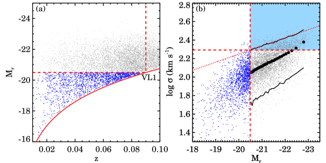
Figure 1.— (a) K-corrected r-band absolute magnitude, $M_{r}$, as a function of redshift for the magnitude limited sample. The solid red curve displays the SDSS spectroscopic survey limit ($r=17.77$). The dashed line shows the boundary for volume-limited sample (VL1) with $0.01<z<0.09$ and $M_{r}<-20.49$. Blue points indicate the objects excluded from VL1. (b) $\sigma$ vs. $M_{r}$ for the magnitude limited sample. The red vertical dashed line shows the magnitude limit of VL1. Black circles and solid curves show the median $\sigma$ and the limits of the central 95% of the $\sigma$ distribution, respectively. The red dotted line is the fit to the upper 95% limit. The $\sigma$ value of the intersection is the $\sigma$ completeness limit ($\sigma_{lim}$, horizontal dashed line) at the maximum redshift of VL1, $z_{max}=0.09$. For $\sigma<\sigma_{lim}$, a significant fraction of galaxies are fainter than $M_{r,lim}$. In other words, VL1 only samples the full $\sigma$ distribution at each $M_{r}$ in the shaded region. We display only 5% of the data for clarity.

Figure 1 (a) shows $M_{r}$ as a function of redshift for galaxies in the magnitude limited sample. The solid line displays the apparent magnitude limit, $r<17.77$, where the SDSS spectroscopic survey is complete ($\sim 95\%$, Strauss et al., 2002). A conventional volume limited sample includes every galaxy brighter than the $M_{r}$ limit ($M_{r,lim}$) of the sample within the volume limited by the redshift $z_{max}$. $M_{r,lim}$ is the $M_{r}$ where the magnitude limited sample is complete at $z_{max}$. The dashed lines in Figure 1 (a) show the boundary of an example volume limited sample (VL1) with $0.01\leq z\leq 0.09$ and $M_{r}\leq M_{r,lim}=-20.49$. Within this volume, VL1 contains all galaxies brighter than $M_{r}\leq-20.49$. A luminosity function derived from VL1 is then complete to $M_{r}=-20.49$.

Figure 1 (b) shows $\sigma$ versus $M_{r}$ for galaxies in the magnitude limited sample. In general, $\sigma$ increases with luminosity, but the $\sigma$ distribution at a given $M_{r}$ is very broad (see also Figure 14 in Sohn et al., 2017). For example, a galaxy at the limiting magnitude $M_{r}=-20.49$ can have $\sigma$ ranging from $\sim 50~{}\rm km~{}s^{-1}$ to $\sim 200~{}\rm km~{}s^{-1}$. Because of the large scatter in $\sigma$, direct conversion from the luminosity limit to a $\sigma$ limit is not trivial (Sheth et al., 2003; Sohn et al., 2017).

A conventional volume limited sample is only complete to the $M_{r}$ limit, not to any $\sigma$ limit. The vertical dashed line in Figure 1 (b) shows the $M_{r}$ limit of VL1. Because of the broad $\sigma$ distribution at fixed $M_{r}$, the sample includes many low $\sigma$ galaxies (e.g., $\log\sigma<2.0$). The VL1 sample also excludes galaxies with $\log\sigma>2.0$ below the $M_{r}$ limit. Blue points in Figure 1 show the faint galaxies that are excluded from VL1. The fraction of these excluded objects is significant for $\log\sigma<2.3$. Because of incomplete sampling of these lower luminosity objects, the VDF derived directly from VL1 underestimates the number of objects with $\log\sigma<2.3$.

3.2. Velocity Dispersion Limit as a Function of Redshift

To construct a $\sigma$ complete sample, we derive $\sigma_{lim}(z)$ for the magnitude limited sample. The $\sigma$ completeness limit of the magnitude limited sample depends on redshift just as the $M_{r}$ limit does. We derive the $\sigma$ completeness limit empirically. Several previous studies of the stellar mass functions follow a similar approach in constructing a stellar mass complete sample (Fontana et al., 2006; Pérez-González et al., 2008; Marchesini et al., 2009; Pozzetti et al., 2010; Weigel et al., 2016).

We first derive $\sigma_{lim}$ for a single volume limited sample. In Figure 1 (b), the red solid curves are the empirically determined central 95% completeness limits for the distribution of $\sigma$ in VL1 as a function of $M_{r}$. The blue dotted line is a linear fit to the upper $\sigma$ limit. We determine the intersection of the $M_{r}$ limit (the vertical dashed line) and the fit to the upper $\sigma$ limit; the $\sigma$ value of the intersection (the horizontal dashed line) is the $\sigma$ limit of VL1, $\sigma_{lim,VL1}$. Galaxies fainter than the $M_{r}$ limit of VL1 rarely ($<2.5\%$) appear above this $\sigma_{lim,VL1}$. Thus, VL1 is complete for $\sigma\geq\sigma_{lim,VL1}$. VL1 is a complete subset of the magnitude limited sample to $z_{max}=0.09$. Therefore, $\sigma_{lim,VL1}$ corresponds to the $\sigma$ completeness limit of the magnitude limited sample at $z_{max}=0.09$.

We derive $\sigma_{lim}(z)$ by repeating the $\sigma_{lim}$ determination for a series of volume limited subsamples with different $z_{max}$. For the series of volume limited samples, $z_{max}$ ranges from 0.0125 to 0.10 in intervals of $\Delta z=0.0025$. In these volume limited samples, the $M_{r}$ limit is brighter as $z_{max}$ increases and thus $\sigma_{lim}$ increases. Red circles in Figure 2 show $\sigma_{lim}$ for the series of volume limited samples. The value of $\sigma_{lim}$ changes rapidly for $z<0.03$ mainly due to the small number of galaxies in the volume. We exclude these local galaxies from further analysis. In the redshift range $0.03\leq z\leq 0.10$, the samples are complete for $\log\sigma>\log\sigma_{lim}(z)$ (the shaded area in Figure 2). We fit $\sigma_{lim}(z)$ with a simple polynomial (blue curve)

$$\log\sigma_{lim}(z)=1.62+13.18z-63.38z^{2}.$$ (2)

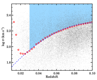
Figure 2.— Velocity dispersion limit (circles) as a function of redshift. The dashed line is a 2nd order polynomial fit to $\sigma_{lim}(z)$. Only galaxies with $\sigma>\sigma_{lim}(z)$ (shaded region) are included in estimating the VDF. We display 20% of the data for clarity.

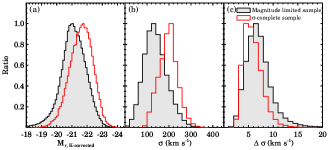
Figure 3.— Properties of galaxies in the magnitude limited sample (filled histogram) and in the $\sigma$ complete sample (open red histogram) including (a) $M_{r}$, (b) $\sigma$ and (c) $\Delta\sigma$.

3.3. Velocity Dispersion Complete Sample

We construct the $\sigma$ complete sample from the magnitude limited sample based on equation 2. We select galaxies by taking only objects with $\sigma>\sigma_{lim}(z)$. The $\sigma$ complete sample consists of 40660 quiescent galaxies in the redshift range $0.03\leq z\leq 0.10$. Figure 3 displays the $M_{r}$, $\sigma$ and observational $\sigma$ uncertainty ($\Delta\sigma$) distributions for galaxies in the $\sigma$ complete sample and in the magnitude limited sample. Galaxies in the $\sigma$ complete sample are brighter and have smaller $\Delta\sigma$s compared to the objects in the magnitude limited sample. The typical $\Delta\sigma$s for galaxies in the $\sigma$ complete sample are $<10~{}\rm km~{}s^{-1}$.

The $\sigma$ complete sample includes 18 galaxies with $\sigma>400~{}\rm km~{}s^{-1}$, extreme for field galaxies. Among these, five objects have $\sigma$ measurements with very large $\Delta\sigma$s ($\gtrsim 100~{}\rm km~{}s^{-1}$). Six objects show merging feature in the SDSS images. The merging feature may affect the central velocity dispersion measurements through the fiber. The remaining seven galaxies are bright elliptical galaxies without signs of disks. These seven galaxies reside in known groups or clusters listed in the NASA Extragalactic Database (NED).

The $\sigma$ complete sample represents the general field sample and includes galaxies in cluster regions according to the cluster abundance in the volume surveyed. We estimate the fraction of cluster galaxies in the $\sigma$ complete sample based on the CIRS cluster catalog (Rines & Diaferio, 2006). The CIRS cluster catalog includes X-ray detected galaxy clusters in the SDSS DR4 with a sky coverage of 4783 deg² ($\sim 60\%$ of the SDSS DR12). The CIRS catalog provides a well-defined sample of spectroscopically identified galaxy clusters.

There are 64 CIRS clusters in the redshift range of the $\sigma$ complete sample. We count the number of galaxies in the $\sigma$ complete sample that are candidate members of the CIRS clusters. We identify the candidate members with $R_{cl}<R_{200}$ and $|\Delta cz|/(1+z_{cl})<2000~{}\rm km~{}s^{-1}$, where $R_{cl}$ is a distance of galaxy from the cluster center, $R_{200}$ is the cluster radius at 200 times critical density, $z_{cl}$ is the cluster redshift. The radial velocity difference limit reflects the maximum amplitude of the caustics for the CIRS clusters (Rines & Diaferio, 2006). We find that 708 galaxies in the $\sigma$ complete sample are possible members of the CIRS clusters. If the cluster abundance is similar in DR12, the total number of galaxies possibly in cluster regions is $\sim 1188$ objects (= $708\times\Omega_{DR12}/\Omega_{DR4}$). Thus, the overall fraction of cluster galaxies in the $\sigma$ complete sample is $\sim 3\%$. The contribution of cluster galaxies increases at greater $\sigma$ (e.g. it is $\sim 5\%$ at $\sigma>250~{}\rm km~{}s^{-1}$).

4. METHOD FOR CONSTRUCTING THE VELOCITY DISPERSION FUNCTION

There are several methods for measuring the statistical distribution function of a galaxy property (i.e., luminosity, stellar mass and velocity dispersion functions) over a wide redshift range. These methods include the classical 1/V_max method (Schmidt, 1968), the parametric maximum likelihood method (Sandage et al., 1979, STY), and the non-parametric maximum likelihood method (Efstathiou et al., 1988). Several studies review the impact of the different methods on the resulting shape of the luminosity and/or the stellar mass functions (Willmer, 1997; Takeuchi et al., 2000; Weigel et al., 2016).

The statistical methods require different basic assumptions. For example, results based on the 1/$V_{max}$ method can be biased if large scale inhomogeneities dominate the sample. Application of the STY method requires a prior functional form for the distribution function.

We employ the stepwise maximum likelihood (SWML) method introduced by Efstathiou et al. (1988). This non-parametric method is powerful because it is less biased in the presence of inhomogeneities in galaxy distribution than the 1/V_max method. The SWML method also has the advantage that a prior functional form of the velocity dispersion function is unnecessary.

The velocity dispersion function derived according to the SWML method can be described as (Efstathiou et al., 1988; Takeuchi et al., 2000; Weigel et al., 2016)

$$\Phi_{k}d\log\sigma=\sum^{N_{gal}}_{i=1}W(\log\sigma_{k}-\log\sigma_{i})\\ \times\bigg{[}\sum^{N_{gal}}_{i=1}\frac{H(\log\sigma_{k}-\log\sigma_{lim,i})}{\sum^{N_{bin}}_{j=1}\Phi_{j}d\log\sigma H(\log\sigma_{j}-\log\sigma_{lim,i})}\bigg{]}^{-1},$$ (3)

where $W(x)$ and $H(x)$ are step functions defined as

$$W(x)=\begin{cases}1&\text{for}~{}-\frac{\Delta\log\sigma}{2}\leq x\leq\frac{\Delta\log\sigma}{2}\\ 0&\text{otherwise},\end{cases}$$ (4)

$$H(x)=\begin{cases}0&\text{for}~{}x<-\frac{\Delta\log\sigma}{2}\\ \frac{x}{\Delta\log\sigma}+\frac{1}{2}&\text{for}~{}-\frac{\Delta\log\sigma}{2}\leq x\leq\frac{\Delta\log\sigma}{2}\\ 1&\text{for}~{}x>\frac{\Delta\log\sigma}{2}.\end{cases}$$ (5)

Here, $N_{gal}$ is the total number of galaxies in the sample, $N_{bin}$ is the number of $\sigma$ bins, $\sigma_{j}$ is the central $\sigma$ of the $\sigma$ bin $j$ and $\sigma_{lim,i}$ is the minimum $\sigma$ that the $i$th galaxy can have and still be found in the sample (see Table 1 for summary). We calculate $\sigma_{lim,i}$ for individual galaxies using equation 2.

Following Efstathiou et al. (1988), we also apply a constraint

$$g=\sum_{k}\Phi_{k}\Delta\log\sigma(\log\sigma_{k}-\log\sigma_{f})^{\beta}-1=0,$$ (6)

where $\log\sigma_{k}$ is the log of the mean $\sigma$ for each bin and $\log\sigma_{f}$ is the log of a fiducial $\sigma$ and $\beta$ is a constant. We choose $\beta=1.5$ following Efstathiou et al. (1988) and set $\log\sigma_{f}=1.0$ following Weigel et al. (2016) who set a small fiducial stellar mass when they measure the stellar mass function based on the SWML method. We derive the errors from the covariance matrix following Efstathiou et al. (1988) (more details are in Ilbert et al., 2005; Weigel et al., 2016). We take the normalization $\Phi_{*}$ of the VDF following Takeuchi et al. (2000) and Weigel et al. (2016)

$$\Phi_{*}=\frac{1}{V_{\rm total}}\sum^{N_{gal}}_{i}\frac{1}{\int^{\infty}_{\log\sigma_{lim,i}}\Phi~{}d\log\sigma}.$$ (7)

Here, $V_{\rm total}$ is the volume of the sample

$$V_{\rm total}=\frac{4\pi}{3}\frac{\Omega_{\rm survey}}{\Omega_{\rm all~{}sky}}\bigg{[}d_{c}(z^{\prime}_{max})^{3}-d_{c}(z^{\prime}_{min})^{3}\bigg{]}.$$ (8)

Here, $\Omega_{\rm survey}~{}(=8032~{}{\rm deg}^{2})$ is the solid angle of the SDSS survey, $\Omega_{\rm all~{}sky}~{}(=40253~{}{\rm deg}^{2})$ is the solid angle of the full sky and $d_{c}(z)$ is a comoving distance at redshift $z$. $z^{\prime}_{min}~{}(=0.03)$ and $z^{\prime}_{max}~{}(=0.10)$ are the lower and upper redshift limit of the $\sigma$ complete sample, respectively.

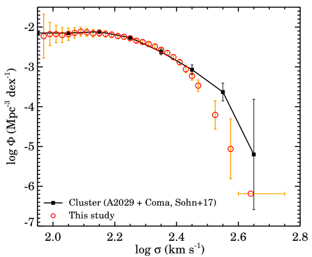
Figure 4.— VDF for the $\sigma$ complete sample (red circles) compared with the cluster VDF (black squares, the sum of Coma and A2029 VDFs, Sohn et al., 2017). We arbitrarily scale the cluster VDF to compare the shapes of the two functions.

Figure 4 shows the VDF for the $\sigma$ complete sample; the field VDF. Table 3 lists the data points for the field VDF. The most massive point marks the seven galaxies with $\sigma>400~{}\rm km~{}s^{-1}$. The horizontal error bar displays the minimum and maximum $\sigma$ for these galaxies. We plot the cluster VDF from Sohn et al. (2017) for comparison. Sohn et al. (2017) measure the cluster VDF of Coma and A2029 using the spectroscopically identified members within $R_{cl}<R_{200}~{}(\sim 2.0$ Mpc). They use the same quiescent galaxy selection $D_{n}4000>1.5$ and $\sigma$s corrected to the fiducial aperture 3 kpc. The VDFs for Coma and A2029 are essentially identical over the range $2.0<\log\sigma<2.6$ (Figure 15 in Sohn et al., 2017).

Table 3Field Velocity Dispersion Function

$\log\sigma$	$\Phi(\Sigma)$	$\Phi$ error
($\rm km~{}s^{-1}$)	(10-3 Mpc-3 dex-1)	(10-3 Mpc-3 dex-1)
1.97	5.911	7.487
1.99	6.687	4.500
2.01	6.686	3.360
2.03	6.297	2.696
2.05	6.617	2.396
2.07	7.152	2.179
2.09	7.671	1.974
2.11	7.358	1.722
2.13	6.987	1.511
2.15	7.024	1.360
2.17	6.715	1.217
2.19	6.445	1.077
2.21	5.954	0.921
2.23	5.709	0.803
2.25	5.216	0.674
2.27	4.547	0.545
2.29	4.221	0.449
2.31	3.743	0.371
2.33	3.270	0.345
2.35	2.685	0.313
2.37	2.248	0.286
2.39	1.757	0.253
2.41	1.315	0.219
2.43	0.872	0.178
2.45	0.593	0.147
2.47	0.338	0.111
2.53	0.062	0.051
2.58	0.009	0.015
2.68	0.001	7.118

5. Discussion

We compare the VDF we measure to the VDF derived from volume limited samples to understand systematic issues from the sample selection (Section 5.1). We compare our result with previous field VDFs (Figure 7, Section 5.2) and with the cluster VDF (Section 5.3). We comment on theoretical considerations (Section 5.4).

5.1. $\sigma$ complete sample vs. volume limited sample

A critical step in measuring the VDF is the use of a $\sigma$ complete sample. The $\sigma$ complete sample includes every galaxy with $\sigma>\sigma_{lim}(z)$ in the magnitude limited sample. We examine the impact of the use of the $\sigma$ complete sample by comparing our measured VDF (Section 4) with the result from a purely volume limited sample.

Figure 5 shows the comparison between the $\sigma$ complete VDF and a VDF derived from the volume limited sample, VL2. VL2 covers the redshift range $0.03\leq z\leq 0.09$ and $M_{r}\leq-20.49$ (Table 2). The VDF for VL2 is the number of galaxies in each $\sigma$ bin divided by the volume of the sample. The VDFs for the $\sigma$ complete and the VL2 samples are similar for $\log\sigma>2.2$. However, the VDF for the $\sigma$ complete sample remains flat for $\log\sigma<2.2$ whereas the VDF for VL2 declines as a result of incomplete sampling of the $\sigma$ distribution at every $M_{r}$.

VL2 is only complete for $\sigma>\sigma_{lim,VL2}~{}(=\log\sigma\gtrsim 2.3$), not for $\log\sigma\sim 2.0$. At $\log\sigma<2.3$, VL2 is incomplete because galaxies fainter than $M_{r,lim}$ but with $\sigma$ in this range are removed from the sample. Figure 6 (a) directly compares the distribution of $\sigma$ for the VL2 sample and the $\sigma$ complete sample as a function of $M_{r}$. VL2 does not completely sample the $\sigma$ distribution below $\sigma_{lim}$. VL2 is more incomplete at lower $\sigma$ because more and more of these galaxies are fainter than $M_{r,lim}$. This incomplete sampling produces the downturn in the VDF for VL2.

The VDF for VL2 appears comparable with the VDF for the $\sigma$ complete sample to $\log\sigma\sim 2.2$ rather than to $\log\sigma\sim 2.3$, the $\sigma_{lim,VL2}$. Figure 6 (b) shows $\sigma$ as a function of redshift for VL2 and for the $\sigma$ complete sample. At $\log\sigma<2.3$, VL2 samples galaxies with $\sigma<\sigma_{lim}(z)$; these objects are excluded from the $\sigma$ complete sample. These galaxies contribute to the VDF measurement based on VL2 and make the VDF decline less rapidly. Thus, although the VDFs for VL2 and the $\sigma$ complete sample have similar shape to $\log\sigma\sim 2.2$, the VDFs are actually derived from somewhat different galaxy samples.

VDFs measured from the various volume limited samples with different $z_{max}$ also decline in the low $\sigma$ regime, but the downturns occur at different $\sigma$s. Volume limited samples with lower $z_{max}$ have fainter $M_{r,lim}$ and are thus more complete to lower $\sigma$. For example, the VDF for a volume limited sample with $z_{max}=0.04$ appears complete to $\log\sigma\sim 2.0$. This VDF for a local volume limited sample also contains galaxies brighter than $M_{r,lim}$ but with $\sigma<\sigma_{lim}$.

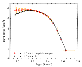
Figure 5.— VDFs for the $\sigma$ complete sample (red circles) and for VL2 (black squares).

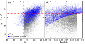
Figure 6.— (a) $\sigma$ as a function of $M_{r}$ for VL2 (grey) and for the $\sigma$ complete sample (blue), respectively. The vertical dashed line shows the magnitude limit ($M_{r,lim}$) of VL2. The objects in the $\sigma$ complete sample that are fainter than the magnitude limit make the VDF flat at low $\sigma$ end. The horizontal dashed line displays the $\sigma$ completeness limit ($\sigma_{lim}$) of VL2 (equation 2). (b) $\sigma$ for the samples as a function of redshift. The symbols are the same as in the left panel. We plot 20% of the data for clarity.

5.2. Comparison with Other Field VDFs

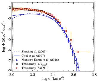
Figure 7.— Comparison between the field VDF for the $\sigma$ complete sample and previous field VDFs. Black squares and red circles display the field VDF for the $\sigma$ complete sample derived with the $1/V_{max}$ and the SWML method, respectively. Dashed and solid lines show SDSS result (Sheth et al., 2003; Choi et al., 2007), and blue triangles show the BOSS result (Montero-Dorta et al., 2017), respectively.

Figure 7 compares the $\sigma$ complete VDF with previous field VDFs derived from SDSS (Sheth et al., 2003; Choi et al., 2007) and BOSS (Montero-Dorta et al., 2017). We plot the previous field VDFs based on the fitting parameters for the ‘modified’ Schechter function (equation (4) in Sheth et al., 2003) given in the literature. We note that the BOSS VDF is limited to $\log\sigma>2.35$ (blue squares). There are several other published field VDFs including Mitchell et al. (2005), Chae (2010) and Bezanson et al. (2011). However, we compare our results only with other results based on spectroscopic determinations of $\sigma$.

The field VDFs in Figure 7 are almost identical for $\log\sigma>2.3$. The $\sigma$ complete VDF slightly exceeds the other SDSS VDFs; this subtle discrepancy may result from different sample selection including the SDSS data release that we use and the difference in quiescent galaxy selection. The slopes of the VDFs are consistent in the high $\sigma$ region regardless of the sample and the quiescent galaxy classification. The VDF measurement across samples and techniques is thus robust for $\log\sigma>2.3$.

The most striking feature in the comparison between field VDFs is the significant difference for $\log\sigma<2.3$. All previous field VDFs decline for $\log\sigma<2.3$; our field VDF remains flat. The slope for $\log\sigma<2.3$ varies among the previous VDFs. The VDF from Choi et al. (2007) is flatter than the VDF from Sheth et al. (2003). Choi et al. (2007) suggest that some morphologically identified early-type galaxies in their sample that are not included the spectroscopically identified early-type samples of Sheth et al. (2003) possibly account for the flatter slope.

Although a detailed analysis of the impact of sample selection is beyond the scope of this paper, a preliminary analysis suggests that the form and parameters of the VDF actually have little sensitivity to the sample selection. For example, selection of quiescent galaxies with Sersic index $\geq 3$ yields a VDF indistinguishable from the results contained here. A color selected red sequence also yields similar results. There may well be subtle dependencies on selection which require a full detailed analysis. Our main goal here is to demonstrate that the field and cluster VDF are indistinguishable when the objects are selected in an identical manner.

The method for deriving the VDF may also affect the shape of the VDF. We measure the field VDF using the SWML method. Previous studies use different methods. Sheth et al. (2003) use the classical $1/V_{max}$ method and Choi et al. (2007) count the number of galaxies in $\sigma$ bins divided by the survey volume.

To examine the impact of different methods for deriving VDF, we compute the VDF for the $\sigma$ complete sample using the $1/V_{max}$ method. The resulting VDF is generally consistent with the VDF derived from the SWML method. The only difference is that the $1/V_{max}$ VDF slightly exceeds the SWML VDF at $\log\sigma<2.05$ (Figure 7). This result is consistent with the conclusion of Weigel et al. (2016) who measure the stellar mass functions using the $1/V_{max}$ and SWML methods. The stellar mass function derived by applying the $1/V_{max}$ exceeds the SWML result at the low mass end. We conclude that the use of the SWML method cannot explain the difference in the field VDFs for $\log\sigma<2.3$.

We measure the VDF based on the $\sigma$ complete sample; previous VDFs are based on volume limited samples (Choi et al., 2007) or magnitude limited samples after correction for incompleteness (Sheth et al., 2003; Montero-Dorta et al., 2017). The previous field VDFs show similar behavior to the VDFs we derive from purely volume limited samples in Section 5.1. This result suggests that the downturns in previous field VDFs may result from incomplete sampling of the $\sigma$ distribution at every $M_{r}$.

5.3. Comparison with Cluster VDFs

The field VDF we derive and the cluster VDF are based on identical sample selection. The field and cluster VDFs are both remarkably flat for $\log\sigma<2.3$ (Figure 4). Sohn et al. (2017) argue that the cluster VDF is a lower limit for $\log\sigma<2.3$ because low surface brightness objects are missing from the sample. The field VDF may also be affected by missing low surface brightness galaxies.

The cluster VDF exceeds the field VDF for $\log\sigma>2.4$. Note that the field VDF also includes a small fraction ($\sim 3\%$) of cluster galaxies, and the contribution of cluster galaxies is larger at greater $\sigma$. Thus, the gap between the cluster and the field VDFs would be even larger if we excluded cluster galaxies from our sample. Sohn et al. (2017) first observed the excess in the cluster VDF. They suggest that the presence of BCGs and other very massive objects, which are relatively rare in field samples, produces this excess in the cluster VDF.

Figure 8 (a) displays the distribution of $\Delta\sigma$ for galaxies with $\log\sigma>2.4$ in both the field and the cluster samples. There is no significant difference in the $\Delta\sigma$ distributions. Coma galaxies tend to have somewhat smaller $\Delta\sigma$s. Because of the proximity of Coma, Coma galaxies at fixed $\sigma$ are generally brighter than their counterparts in the A2029 and in the field samples. $\Delta\sigma$s for $\log\sigma>2.4$ are $\lesssim 10~{}\rm km~{}s^{-1}$, less than the size of $\sigma$ bin ($\sim 15~{}\rm km~{}s^{-1}$) we use for measuring the VDF. Thus, the shape of the VDFs and the excess in the cluster VDF for $\log\sigma>2.4$ are not significantly affected by the error distribution.

Figure 8 (b) shows the $D_{n}4000$ distributions for the field and the cluster samples. The cluster samples tend to have larger $D_{n}4000$ (see also Figure 13 in Sohn et al., 2017). The $D_{n}4000$ is the indicator of stellar population of ages and the cluster objects tend to be older than the field objects. This result is consistent with the correlation between $\sigma$ and $D_{n}4000$ (Zahid & Geller, 2017).

The excess of the cluster VDF at high $\sigma$ implies that there may be a fundamental difference in the relative abundance of galaxies with $\log\sigma>2.4$ in the field and cluster environments. The shallower cluster VDF implies that the clusters preferentially contain a larger number of high $\sigma$ galaxies than the typical field. Each cluster has a dominant central galaxy (brightest cluster galaxy, BCG) generally with $\log\sigma>2.4$ (Lauer et al., 2014). However, the excess in the cluster VDF cannot be explained by a single BCG in each cluster. Fifteen galaxies with $\log\sigma>2.4$ make the slope of the cluster VDF shallower at $\log\sigma>2.4$.

Clusters often consist of several subclusters each with its own BCG. Their presence reflects the hierarchical formation process. High $\sigma$ galaxies that develop in the individual subclusters may contribute to the excess in the cluster VDF. For example, the multiple BCGs within several substructures in the Coma cluster (Colless & Dunn, 1996; Tempel et al., 2017) may support this picture. Analysis of cluster VDFs in concert with substructure analysis for a large set of clusters should further elucidate this issue.

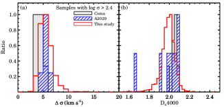
Figure 8.— (a) $\Delta\sigma$ distributions and (b) $D_{n}4000$ distributions for galaxies with $\log\sigma>2.4$. The red open histogram shows the distributions for the $\sigma$ complete sample, the filled and hatched histograms show the same for Coma and A2029 members, respectively.

5.4. Comparison with Simulations

VDFs provide an interesting probe for modeling structure formation because $\sigma$ may be a good proxy for the DM subhalo mass (Wake et al., 2012a, b; Bogdán & Goulding, 2015; Zahid et al., 2016). Here we compare VDFs for the field and for two massive clusters. The difference between the field and cluster VDFs for $\log\sigma>2.4$ is a potential test of models for the formation of galaxies in clusters.

Theoretical model VDFs have not yet been computed in a way that mimics the observations. Munari et al. (2016) investigate the $\sigma$ distribution of a rich cluster A2142 based on $\sigma$s from the SDSS and compare their result with simulations. They suggest that numerical simulations significantly underestimate the number of massive subhalos. In fact, they compare the distribution of circular velocities of galaxies in the observations and the simulations because measuring circular velocities is straightforward in simulations. To derive the circular velocity distribution for the observations, they convert the observed central velocity dispersions into circular velocities. This conversion makes reasonable assumptions, but a direct comparison of central $\sigma$s would provide more powerful constraints.

Currently there are no VDFs derived from simulations that mimic the observations. To do this, the velocity dispersions for subhalos in the simulations must be measured in a cylinder through the center of the subhalo mimicking the $\sigma$ we measure observationally. Comparison with the observed field VDFs requires model VDFs derived from hydrodynamic large-scale cosmological simulations with high resolutions like Illustris (Vogelsberger et al., 2014), EAGLE (Schaye et al., 2015), and MassiveBlack-II (Khandai et al., 2015). These simulations identify galaxies with stellar mass $>10^{9}M_{\odot}$ and thus the VDF from this simulations could in principle be measured for $\log\sigma>2.0$. Several studies do calculate the projected radial velocity dispersions for objects in cosmological hydrodynamic simulations (Choi & Yi, 2017; Penoyre et al., 2017). Their velocity dispersion measurements mimic IFU observations, but they do not provide $\sigma$ in fixed metric apertures. Velocity dispersions measured within circular apertures could be derived from these simulations and would be the best benchmark for direct comparison with the observed VDFs. The combinations of observed and simulated VDFs are a potentially important window for understanding the halo mass distribution.

6. CONCLUSION

We measure the field VDF for a $\sigma$ complete sample in the range $\log\sigma>2.0$. The $\sigma$ complete sample includes field quiescent galaxies with $D_{n}4000>1.5$ and $\sigma$ measured within a 3 kpc aperture, just like the cluster sample used for measuring the cluster VDF (Sohn et al., 2017).

The $\sigma$ complete sample we construct includes every galaxy with $\sigma$ larger than the $\sigma$ completeness limit of the SDSS magnitude limited sample as a function of redshift, $\sigma_{lim}(z)$. We estimate the $\sigma$ complete limit of the magnitude limited sample empirically to construct the $\sigma$ complete sample. The method we use to construct the $\sigma$ complete sample can be applied more generally to construct samples complete in any other observables from a magnitude limited survey.

The VDF for the $\sigma$ complete sample is much flatter than the VDF for purely volume limited sample for $\log\sigma<2.2$. The $\sigma$ complete sample includes faint low $\sigma$ galaxies below the $M_{r,lim}$ of the volume limited sample. The sampling of these galaxies results in the flatter VDF. Previous field VDFs derived from either a purely volume limited sample or a magnitude limited sample also show a downturn for $\log\sigma<2.2$. The incompleteness of these samples in sampling the full $\sigma$ distribution could produce the decline in the previous VDFs at low $\sigma$.

The flat field VDF we derive from the $\sigma$ complete sample is essentially identical to the cluster VDF for $\log\sigma<2.2$. The previous discrepancy in the low $\sigma$ range appears to be completely explained by the use of the $\sigma$ complete sample.

The field VDF is steeper than the cluster VDF for the massive clusters A2029 and Coma for $\log\sigma>2.4$. The difference for $\log\sigma>2.4$ probes the formation and evolution of massive galaxies in the cluster environment and may reflect the presence of these massive objects within cluster substructures.

The VDF is potentially a direct probe of the dark matter subhalo mass distribution. The combination of the cluster VDF from Sohn et al. (2017) and the field VDFs provides benchmarks for testing N-body and hydrodynamic simulations. Measuring $\sigma$ from simulations in a way that mimics the observations would be an important step toward realizing the potential of this test.

References

- Alam et al. (2015) Alam, S., Albareti, F. D., Allende Prieto, C., et al. 2015, ApJS, 219, 12
- Auger et al. (2010) Auger, M. W., Treu, T., Bolton, A. S., et al. 2010, ApJ, 724, 511
- Balogh et al. (1999) Balogh, M. L., Morris, S. L., Yee, H. K. C., Carlberg, R. G., & Ellingson, E. 1999, ApJ, 527, 54
- Bernardi et al. (2010) Bernardi, M., Shankar, F., Hyde, J. B., et al. 2010, MNRAS, 404, 2087
- Bernardi et al. (2013) Bernardi, M., Meert, A., Sheth, R. K., et al. 2013, MNRAS, 436, 697
- Bezanson et al. (2011) Bezanson, R., van Dokkum, P. G., Franx, M., et al. 2011, ApJ, 737, L31
- Blanton et al. (2005) Blanton, M. R., Schlegel, D. J., Strauss, M. A., et al. 2005, AJ, 129, 2562
- Bogdán & Goulding (2015) Bogdán, Á., & Goulding, A. D. 2015, ApJ, 800, 124
- Cappellari & Emsellem (2004) Cappellari, M., & Emsellem, E. 2004, PASP, 116, 138
- Chae (2010) Chae, K.-H. 2010, MNRAS, 402, 2031
- Choi et al. (2007) Choi, Y.-Y., Park, C., & Vogeley, M. S. 2007, ApJ, 658, 884
- Choi & Yi (2017) Choi, H., & Yi, S. K. 2017, ApJ, 837, 68
- Colless & Dunn (1996) Colless, M., & Dunn, A. M. 1996, ApJ, 458, 435
- Croton et al. (2005) Croton, D. J., Farrar, G. R., Norberg, P., et al. 2005, MNRAS, 356, 1155
- Djorgovski & Davis (1987) Djorgovski, S., & Davis, M. 1987, ApJ, 313, 59
- Dressler et al. (1987) Dressler, A., Lynden-Bell, D., Burstein, D., et al. 1987, ApJ, 313, 42
- Evrard et al. (2008) Evrard, A. E., Bialek, J., Busha, M., et al. 2008, ApJ, 672, 122-137
- Efstathiou et al. (1988) Efstathiou, G., Ellis, R. S., & Peterson, B. A. 1988, MNRAS, 232, 431
- Faber & Jackson (1976) Faber, S. M., & Jackson, R. E. 1976, ApJ, 204, 668
- Fabricant et al. (2005) Fabricant, D., Fata, R., Roll, J., et al. 2005, PASP, 117, 1411
- Fabricant et al. (2013) Fabricant, D., Chilingarian, I., Hwang, H. S., et al. 2013, PASP, 125, 1362
- Fontana et al. (2006) Fontana, A., Salimbeni, S., Grazian, A., et al. 2006, A&A, 459, 745
- Geller et al. (2014) Geller, M. J., Hwang, H. S., Fabricant, D. G., et al. 2014, ApJS, 213, 35
- Grillo et al. (2008) Grillo, C., Lombardi, M., & Bertin, G. 2008, A&A, 477, 397
- Ilbert et al. (2005) Ilbert, O., Tresse, L., Zucca, E., et al. 2005, A&A, 439, 863
- Kauffmann et al. (2003) Kauffmann, G., Heckman, T. M., White, S. D. M., et al. 2003, MNRAS, 341, 33
- Khandai et al. (2015) Khandai, N., Di Matteo, T., Croft, R., et al. 2015, MNRAS, 450, 1349
- Lauer et al. (2014) Lauer, T. R., Postman, M., Strauss, M. A., Graves, G. J., & Chisari, N. E. 2014, ApJ, 797, 82
- Maraston & Strömbäck (2011) Maraston, C., & Strömbäck, G. 2011, MNRAS, 418, 2785
- Marchesini et al. (2009) Marchesini, D., van Dokkum, P. G., Förster Schreiber, N. M., et al. 2009, ApJ, 701, 1765
- Mignoli et al. (2005) Mignoli, M., Cimatti, A., Zamorani, G., et al. 2005, A&A, 437, 883
- Mitchell et al. (2005) Mitchell, J. L., Keeton, C. R., Frieman, J. A., & Sheth, R. K. 2005, ApJ, 622, 81
- Montero-Dorta et al. (2017) Montero-Dorta, A. D., Bolton, A. S., & Shu, Y. 2017, MNRAS, 468, 47
- Munari et al. (2016) Munari, E., Grillo, C., De Lucia, G., et al. 2016, ApJ, 827, L5
- Norberg et al. (2001) Norberg, P., Baugh, C. M., Hawkins, E., et al. 2001, MNRAS, 328, 64
- Penoyre et al. (2017) Penoyre, Z., Moster, B. P., Sijacki, D., & Genel, S. 2017, arXiv:1703.00545
- Pérez-González et al. (2008) Pérez-González, P. G., Rieke, G. H., Villar, V., et al. 2008, ApJ, 675, 234-261
- Posti et al. (2014) Posti, L., Nipoti, C., Stiavelli, M., & Ciotti, L. 2014, MNRAS, 440, 610
- Pozzetti et al. (2010) Pozzetti, L., Bolzonella, M., Zucca, E., et al. 2010, A&A, 523, A13
- Rines & Diaferio (2006) Rines, K., & Diaferio, A. 2006, AJ, 132, 1275
- Sánchez-Blázquez et al. (2006) Sánchez-Blázquez, P., Peletier, R. F., Jiménez-Vicente, J., et al. 2006, MNRAS, 371, 703
- Schaye et al. (2015) Schaye, J., Crain, R. A., Bower, R. G., et al. 2015, MNRAS, 446, 521
- Schmidt (1968) Schmidt, M. 1968, ApJ, 151, 393
- Sheth et al. (2003) Sheth, R. K., Bernardi, M., Schechter, P. L., et al. 2003, ApJ, 594, 225
- Sohn et al. (2017) Sohn, J., Geller, M. J., Zahid, H. J., et al. 2017, ApJS, 229, 20
- Sandage et al. (1979) Sandage, A., Tammann, G. A., & Yahil, A. 1979, ApJ, 232, 352
- Strauss et al. (2002) Strauss, M. A., Weinberg, D. H., Lupton, R. H., et al. 2002, AJ, 124, 1810
- Takeuchi et al. (2000) Takeuchi, T. T., Yoshikawa, K., & Ishii, T. T. 2000, ApJS, 129, 1
- Tempel et al. (2017) Tempel, E., Tuvikene, T., Kipper, R., & Libeskind, N. I. 2017, arXiv:1704.04477
- Treu et al. (2006) Treu, T., Koopmans, L. V., Bolton, A. S., Burles, S., & Moustakas, L. A. 2006, ApJ, 640, 662
- Thomas et al. (2013) Thomas, D., Steele, O., Maraston, C., et al. 2013, MNRAS, 431, 1383
- Vergani et al. (2008) Vergani, D., Scodeggio, M., Pozzetti, L., et al. 2008, A&A, 487, 89
- Vogelsberger et al. (2014) Vogelsberger, M., Genel, S., Springel, V., et al. 2014, MNRAS, 444, 1518
- Wake et al. (2012a) Wake, D. A., Franx, M., & van Dokkum, P. G. 2012, arXiv:1201.1913
- Wake et al. (2012b) Wake, D. A., van Dokkum, P. G., & Franx, M. 2012, ApJ, 751, L44
- Weigel et al. (2016) Weigel, A. K., Schawinski, K., & Bruderer, C. 2016, MNRAS, 459, 2150
- Willmer (1997) Willmer, C. N. A. 1997, AJ, 114, 898
- Woods et al. (2010) Woods, D. F., Geller, M. J., Kurtz, M. J., et al. 2010, AJ, 139, 1857
- Zahid et al. (2016) Zahid, H. J., Geller, M. J., Fabricant, D. G., & Hwang, H. S. 2016, ApJ, 832, 203
- Zahid & Geller (2017) Zahid, H. J., & Geller, M. J. 2017, arXiv:1701.01350