Towards Understanding the Impact of Human Mobility on Police Allocation

Abstract

Motivated by recent findings that human mobility is proxy for crime behavior in big cities and that there is a superlinear relationship between the people’s movement and crime, this article aims to evaluate the impact of how these findings influence police allocation. More precisely, we shed light on the differences between an allocation strategy, in which the resources are distributed by clusters of floating population, and conventional allocation strategies, in which the police resources are distributed by an Administrative Area (typically based on resident population). We observed a substantial difference in the distributions of police resources allocated following these strategies, what evidences the imprecision of conventional police allocation methods.

I Introduction

Faced with the ever-growing problem of crime, prevention strategies have come to the fore as a key issue and one of the main challenges of Law Enforcement authorities. This increase has been observed mainly in large urban centers and even with huge masses of digitized data about police activities and reported crimes, the police institutions do not seem to use adequately this information to fight the growth of crime.

Within this context, strategies of police allocation play an important role in crime prevention and a recent discovery by Caminha et al. [1] motivated us to revisit the state of the art of this subject. Caminha et al. discovered a superlinear relationship [2, 3, 4, 5, 6, 7, 8, 9, 10, 11, 12] between the flow of people and property crimes. In other words, the authors found that the increase of the floating population in a urban space implies a disproportionate growth of property crime in that space. Formally this relationship can be represented by the equation $Y=aX^{\beta}$, indicating a Power Law, where $Y$ quantifies property crimes, $X$ quantifies the volume of people flow, $a$ is a normalization constant and $\beta$ is the exponent that scales the relation, which in the case of a superlinear relation is assumed to be $\beta>1$. The authors further assert that administrative territorial units that typically account for features of resident population, such as divisions by neighborhoods, census tracts or zones, are unable to precisely capture the effect that social relations have over crime. This fact has already been stated by several urban indicators in important scientific productions [13, 14, 15, 16, 17, 18, 19, 20, 21].

Although over the years a series of scientific works have studied factors surrounding crime [22, 23, 24, 25, 26, 27, 28, 29], none of them have taken into consideration this finding that quantifies the relation between human mobility and crime. More specifically, they do not make use of the divisions of urban spaces estimated from the floating population to police allocation.

In this article we seek to understand the impact, in the allocation of police resources, from the fact that the relationship between the movement of people and property crimes follows a Power Law. To estimate this impact, we use data from a big metropolis to build clusters of floating population that will be considered as the basis for the allocation strategy. The distribution of the police resources obtained from the application of this strategy is compared to a conventional allocation strategy, in which police officers are distributed into administrative territorial divisions. Doing so, we were able to show the difference between the distribution of allocated police according to the two strategies. This difference allows us to conclude that, under the light of these new evidences of cause-effect between floating population and property crimes, it is inaccurate to apply a conventional strategy of police allocation, which is based only on resident population.

II State of Art

There is a vast selection of literature on police allocation in urban space to combat criminal activity. There was a growing interest in developing techniques using programs of spatial analysis to identify areas where the police resources are to be allocated. In a very general way, a typical strategy of allocation is to implement a heterogeneous model, in which the distribution of resources in a geographic area is directly proportional to the density of crimes of that region. Typically these areas are administrative regions ( e.g. census tract or neighbohoods) demarcated from features of the resident population [30]. This perspective, is not totally in line with routine activity theory [31, 32, 33] and criminal career approaches [34],but ,for practical reasons, have been used for years [35].

With the increase in the volume of digital data and the creation of more sophisticated mapping techniques, opportunities have appeared to go beyond the approaches where only the density of crimes in areas of resident population is considered [36, 37, 38]. Nevertheless, much of the work in this area continued to focus on the concentration of crime in administrative territorial units [39, 40]. It is true that Kennedy et al. [41] developed an in-depth assessment of social factors that contribute to crime occurrence. However, its allocation algorithm is based on risk areas which indirectly are also measured by resident population indicators.

There are also a number of papers that use simulation models to teach the police officer how to make an allocation of quality resources [42, 43, 44, 45, 46]. However, these works do not consider the new evidence that human mobility is the key to understanding the emergence of property crimes in regions of urban space.

Finally, it is worth noting that there are numerous studies that seek to understand phenomena related to human mobility [47, 48, 49, 50, 51], however, works that apply the knowledge obtained from these studies on crime prevention from police allocation is scarce.

III Datasets

In this paper, data on property crimes was used, this was obtained from [52]. In total this dataset contains 81,911 geo-referenced crimes occurring between August 2005 and July 2007. Three levels of segmentation were used for the city of Fortaleza-CE, Brazil. The first level was a division by neighborhood, obtained from [53], in total, Fortaleza has 116 districts spread over an area of 313 $\mathrm{km^{2}}$ where more than 2,400,000 people live. The second level, a division by defined census tracts by IBGE (Brazilian Institute of Geography and Statistics) [54], which divides the city into 3043 subareas that on average contain 800 residents each. Finally, the third level of segmentation, a division by clusters of floating population, estimated in [1]. In total, the authors divided Fortaleza into 119 clusters using City Clustering Algorithm (CCA) [13, 14, 15, 16, 17, 18, 19, 20].

To define the boundaries of this clusters, the CCA algorithm considered the notion of spatial continuity through the aggregation of census tracts that are near one another. The CCA constructs the floating population boundaries of an urban area considering two parameters, namely, a population density threshold, $D^{*}$, and a distance threshold, $\ell$. For the $i\mathrm{-th}$ census tract, the population density $D_{i}$ is located in its geometric center; if $D_{i}>D^{*}$, then the $i\mathrm{-th}$ census tract is considered populated. The length $\ell$ represents a cutoff distance between census tracts to consider them as spatially contiguous, i.e., all of the nearest neighboring census tracts that are at distances smaller than $\ell$ are clustered. Hence, a cluster made by the CCA is defined by populated areas within a distance less than $\ell$, as seen schematically in Figure 1. Previous studies [21, 17, 19] have demonstrated that the results produced by the CCA can be weakly dependent on $D^{*}$ and $\ell$ for some range of parameter values. In [1] $\ell$ was quantified in meters (m) and $D^{*}$ in people passing by $\mathrm{km^{2}}$ in one day.

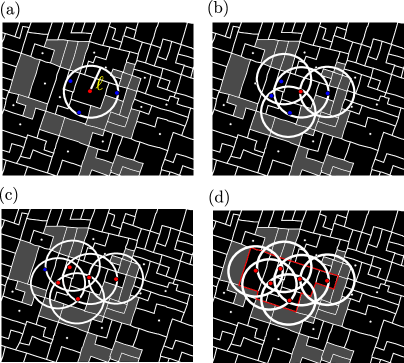
Figure 1: The scheme of the City Clustering Algorithm (CCA). Each square represents a clustering unit, specifically in our case, they represent census tracts. Black squares are candidates for clustering $(D_{i}>D^{*})$, in contrast, the gray squares cannot be clustered ($D_{i}\leq D^{*}$). (a) The red dot represents the geometric center of the $i$-th census tract and the white circle with radius $\ell$ seeks neighbors belonging to the same cluster. (b) The same search operation is made for the other census tracts. (c) The same operation is done until there are no more neighbors within the radius of operation. (d) The algorithm finishes running and the cluster is found.

Figure 2 illustrates the clusters found. The base division used in the cluster was the census tract map. The census tract in light gray color were not grouped because they have low flux density ($D_{i}\leq D^{*}$), the other colors represent clusters found. In the division reached by the CCA the volume of flow of a cluster is proportional to its area [21]. It was estimated $\ell=320$ and $D^{*}=6000$.

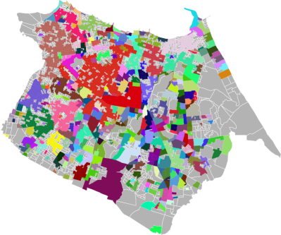
Figure 2: Agglomerates found by the CCA algorithm. The regions in light gray color were not grouped because they have low floating population density ($D_{i}\leq D^{*}$), the other colors represent clusters found. More precisely, each color represents a people flow agglomerate.

IV Methods

Two strategies of police allocation will be compared here, these strategies are based on the most popular heterogeneous allocation model, namely by high crime density. The first, called Resident Population Allocation (RPA) Strategy is a conventional strategy of police allocation, whose resources are distributed in proportion to the quantity of occurrences in administrative divisions of a territory (what is typically estimated from features from the resident population). In this work the division by neighborhood’s boundaries will be adopted, because, despite the division by census tracts being available, it is too segmented, with some of them being less than one block, thus being unfeasible to be used in a real policy of resource allocation.

The second allocation strategy, called Floating Population Allocation (FPA) Strategy, will also distribute police resources proportionally to the number of calls to the police in a spatial division, however, in this strategy the boundaries of the areas follow the clusters of floating population estimated in [1].

In this way, the part of a police resource, $T_{s_{i}}$, allocated to a sub-region of urban space (whether a clusters of floating population or a neighborhoods), $s_{i}$ $\in$ $S$, from the quantity of crimes occurring in $s_{i}$, $C{s_{i}}$, can be formally defined as $T_{s_{i}}=\frac{T*C{s_{i}}}{C}$. Where $T$ is the total number of police officers available for allocation and $C$ is the total number of crimes that have occurred in all the urban space available for allocation.

A policy of internal allocation was also adopted, precisely at the level of $s_{i}$. Each cluster of floating population or neighborhood is composed of census tracts and internally there is also a allocating of resources in a manner proportional to the number of crimes of each census tract within $s_{i}$. In other words, within each sub-region $s_{i}$, sectors with more crimes receive more police officers. This sub-allocation policy is justified by the need to compare the two strategies, which will be discussed later on.

V Results

When applying RPA Strategy and FPA Strategy in Fortaleza to simulate the availability of a total police resource $T=10,000$, the heat maps shown in Figure 3, items (a) and (b), respectively. Hot Spots with more intensity can be seen in FPA Strategy, mainly in the commercial center of the city, highlighted by the black circle in both figures. This is because FPA Strategy does not allocate police resources in areas that are considered uninhabited $(D_{i}>D^{*})$, instead concentrating more police in the most critical regions of the city.

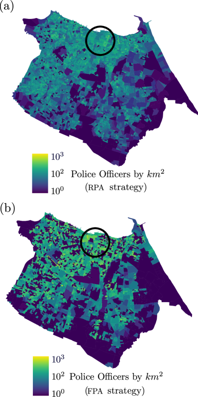
Figure 3: Police allocation using the two strategies studied. (a) shows density map of police allocated using RPA Strategy, (b) shows density map of police allocated using FPA Strategy. Black circles highlight the shopping center of Fortaleza, an area with a large population concentration and consequently, a large concentration of crimes against property.

For the purpose of comparison, the amount of police allocated per neighborhood was calculated using FPA Strategy. Then, the number of police officers in the census tracts located within each neighborhood was added. After this, we calculated the percentage difference of the number of policemen allocated by neighborhood by both strategies. In Figure 4, items (a) and (b) illustrate the neighborhoods where the allocation is more similar and more different respectively.

In general, a greater similarity was observed in the allocations in the neighborhoods with greater presence of fluctuating populations, these neighborhoods are close to the commercial center of the city or located in regions with a high concentration of residents (normally locations that are the source of floating population). It was also observed that the districts that presented a greater percentage difference between the quantities of police officers allocated using the allocation strategies studied, are those which have more non-populated census tracts, that is, with a floating population density below the threshold $D^{*}$, as estimated in [1].

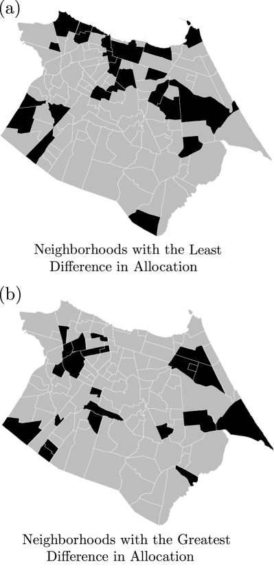
Figure 4: Differences and similarities among the studied allocations. (a) highlights in black the neighborhoods that had the most similar allocation using RPA e FPA Strategy. (b) highlights the neighborhoods with the highest difference in the number of police officers allocated. In both figures 24 neighborhoods are highlighted, 20% of the city total.

In Figure 5 a more detailed comparison can be observed between the two allocation strategies. (a) illustrates the interpolation functions [55] of the neighborhoods by the number of police officers allocated by the two strategies studied. The intersection of the areas formed by interpolation curves and the $x$ axis reveals approximately 15% dissimilarity between the allocations. This dissimilarity can be observed more clearly in Figure 5 (b), where the interpolation functions of the histograms generated from the number of police officers allocated by neighborhoods according to the two strategies is shown. The blue line represents the interpolation function of the RPA Strategy data. The red line represents the estimated function for the FPA Strategy. The regions in light red color represent areas where there was no intersection. Added together, these regions represent 15% of the total area.

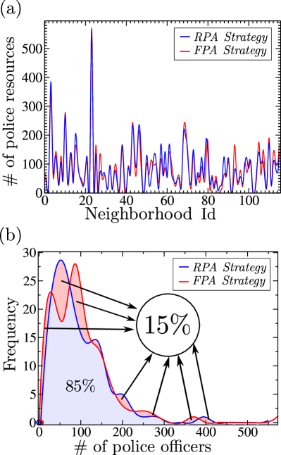
Figure 5: RPA and FPA Strategy statistical comparison. In (a) is illustrated the number of police resources allocated by neighborhood. The blue line represents a Cubic Spline Interpolation [55] applied to the values that was found in RPA Strategy. The red line is the same interpolation applied to the FPA Strategy. (b) show the histograms distribution to the allocations in the neighborhoods of the city. For better visualization, the histograms has been generated in 20 bins [56].

Such difference quantifies the inefficacy of the RPA Strategy. While the allocation produced from the FPA strategy is strongly correlated with the flow of people, the RPA strategy fails to capture the scale found by Caminha et al. [1]. Remember that their studies found a superlinear relationship between property crimes and floating population with exponent $\beta=1.15\pm 0.4$. Figure 6 shows the correlation between the number of police resources allocated and floating population following the two different strategies. In (a) it is shown the correlation between the resources allocated and floating population following the FPA strategy. There is a clear superlinear relation with an exponent of $\beta=1.18\pm 0.05$ and a strong coefficient of determination [57, 58] ($R^{2}=0.83$), On the other hand, in (b), although a superlinear relation appears, the determination coefficient ($R^{2}=0.70$) as well as the standard error of this [57, 58] ($\pm 0.11$) reveals that the RPA Strategy is not the more adequate to the city of Fortaleza. Another important feature that indicates the inappropriateness of the RPA strategy is also observed in Figure 6, specifically the analysis of the dispersion of the dots (clusters). In (b), we can see four clusters of floating population with considerable activity (flow of people) with few police resources. This happens because the boundaries between neighborhoods sometimes divide the floating clusters what makes difficult a precise allocation of resource in that region. In general, although the RPA strategy suggests the distribution of resources in a way that follows a Power Law, there is an imprecision because this strategy aims at capturing the influence of floating population indirectly via the incidence of crime. That is to say, as crime occurs due to the presence of people, looking at crime is a way to consider the floating population. This is not however the best approach because it fails to capture the potential of occurrence of crime in a disproportional way caused by the existence of clusters of floating population. When the FPA Strategy is applied the cause (flow of people in a region) and the amount of crime are considered to determine the amount of resources to be allotted. Doing so, it is possible to statistically approximate (in terms of exponent and standard error) the superlinear relation as suggested by Caminha et al. [1].

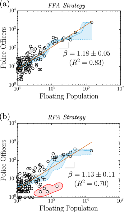
Figure 6: Correlations between police officers and floating population in RPA and FPA Strategy. (a) and (b), respectively, illustrates the correlations achieved for RPA and FPA Strategy. The $x$-axis represents the floating population and $y$-axis the number of police officers allocated. The red lines represent the simple linear regressions applied to the data, the blue continuous lines represent the Nadaraya-Watson method [59, 60] and the blue dashed lines delimit the 95% confidence interval (CI) estimated by bootstrap

.

VI Conclusion

This paper presented a study that investigates new ways of allocating police resources within the urban space. Differently to conventional allocation policies, which allocate resources through the city using administrative units , an allocation strategy was presented which distributes police by clusters of floating population, which have already been proved to be much more precise in explaining the behavior of crimes against property in a city [1]. This precision is due to the fact that the borders of population flux often go beyond the boundaries of the administrative divisions and clustering algorithms identify the ”islands” formed by those clusters that are naturally strategic regions in combating crime.

Our study reveals that allocation of police resources into clusters of floating population leads the distribution of resources in a way significantly different from strategies that allocates resources having per basis the administrative regions. More specifically, we show that the allocation having as basis the clusters of floating population tends to be more adequate for fighting crime against properties because the distribution of police resources will naturally follow a Power Law, what is desirable since it is expected that crime grows disproportionally in areas with high density of floating population.

The aspects discussed here open new lines of further investigations. In particular, it is important to notice that the work by Caminha et al. has also shown that for certain types of crimes (e.g. peace disturbance) the superlinear relationship is only captured having as basis administrative areas that account for features of resident population rather than clusters of floating population. This indicates that it is necessary to think in a hybrid strategy in which different polices and different divisions of the urban space need to be taken into consideration for each type of crime.

References

- [1] C. Caminha, V. Furtado, T. H. Pequeno, C. Ponte, H. P. Melo, E. A. Oliveira, and J. S. Andrade Jr, “Human mobility in large cities as a proxy for crime,” PLoS One, vol. 2, no. 12, p. e0171609, 2017.
- [2] L. M. Bettencourt, J. Lobo, D. Strumsky, and G. B. West, “Urban scaling and its deviations: Revealing the structure of wealth, innovation and crime across cities,” PloS One, vol. 5, no. 11, p. e13541, 2010.
- [3] A. Gomez-Lievano, H. Youn, and L. M. Bettencourt, “The statistics of urban scaling and their connection to zipf’s law,” PLoS One, vol. 7, no. 7, p. e40393, 2012.
- [4] C. A. Ignazzi, “Scaling laws, economic growth, education and crime: evidence from brazil,” L’Espace géographique, vol. 43, no. 4, pp. 324–337, 2014.
- [5] Q. S. Hanley, D. Lewis, and H. V. Ribeiro, “Rural to urban population density scaling of crime and property transactions in english and welsh parliamentary constituencies,” PloS One, vol. 11, no. 2, p. e0149546, 2016.
- [6] L. G. Alves, R. S. Mendes, E. K. Lenzi, and H. V. Ribeiro, “Scale-adjusted metrics for predicting the evolution of urban indicators and quantifying the performance of cities,” PloS One, vol. 10, no. 9, p. e0134862, 2015.
- [7] E. Arcaute, E. Hatna, P. Ferguson, H. Youn, A. Johansson, and M. Batty, “Constructing cities, deconstructing scaling laws,” Journal of The Royal Society Interface, vol. 12, no. 102, p. 20140745, 2015.
- [8] E. Arcaute, C. Molinero, E. Hatna, R. Murcio, C. Vargas-Ruiz, A. P. Masucci, and M. Batty, “Cities and regions in britain through hierarchical percolation,” Open Science, vol. 3, no. 4, p. 150691, 2016.
- [9] C. Cottineau, O. Finance, E. Hatna, E. Arcaute, and M. Batty, “Defining urban agglomerations to detect agglomeration economies,” arXiv preprint arXiv:1601.05664, 2016.
- [10] J. C. Leitão, J. M. Miotto, M. Gerlach, and E. G. Altmann, “Is this scaling nonlinear?,” Royal Society Open Science, vol. 3, no. 7, 2016.
- [11] L. M. Bettencourt, “The origins of scaling in cities,” science, vol. 340, no. 6139, pp. 1438–1441, 2013.
- [12] S. Arbesman, J. M. Kleinberg, and S. H. Strogatz, “Superlinear scaling for innovation in cities,” Physical Review E, vol. 79, no. 1, p. 016115, 2009.
- [13] H. A. Makse, J. S. Andrade, M. Batty, S. Havlin, H. E. Stanley, et al., “Modeling urban growth patterns with correlated percolation,” Physical Review E, vol. 58, no. 6, p. 7054, 1998.
- [14] H. D. Rozenfeld, D. Rybski, J. S. Andrade, M. Batty, H. E. Stanley, and H. A. Makse, “Laws of population growth,” Proceedings of the National Academy of Sciences, vol. 105, no. 48, pp. 18702–18707, 2008.
- [15] K. Giesen, A. Zimmermann, and J. Suedekum, “The size distribution across all cities–double pareto lognormal strikes,” Journal of Urban Economics, vol. 68, no. 2, pp. 129–137, 2010.
- [16] H. D. Rozenfeld, D. Rybski, X. Gabaix, and H. A. Makse, “The area and population of cities: New insights from a different perspective on cities,” The American Economic Review, vol. 101, no. 5, pp. 2205–2225, 2011.
- [17] G. Duranton and D. Puga, “The growth of cities,” 2013.
- [18] L. K. Gallos, P. Barttfeld, S. Havlin, M. Sigman, and H. A. Makse, “Collective behavior in the spatial spreading of obesity,” Scientific reports, vol. 2, 2012.
- [19] G. Duranton, “Delineating metropolitan areas: Measuring spatial labour market networks through commuting patterns,” in The Economics of Interfirm Networks, pp. 107–133, Springer, 2015.
- [20] J. Eeckhout, “Gibrat’s law for (all) cities,” The American Economic Review, vol. 94, no. 5, pp. 1429–1451, 2004.
- [21] E. A. Oliveira, J. S. Andrade Jr, and H. A. Makse, “Large cities are less green,” Scientific reports, vol. 4, 2014.
- [22] H. P. M. Melo, A. A. Moreira, É. Batista, H. A. Makse, and J. S. Andrade, “Statistical signs of social influence on suicides,” Scientific reports, vol. 4, 2014.
- [23] A. Gelman, J. Fagan, and A. Kiss, “An analysis of the new york city police department’s “stop-and-frisk” policy in the context of claims of racial bias,” Journal of the American Statistical Association, vol. 102, no. 479, pp. 813–823, 2007.
- [24] R. Agnew, “Pressured into crime: An overview of general strain theory,” 2007.
- [25] C. Caminha and V. Furtado, “Modeling user reports in crowdmaps as a complex network,” in Proceedings of 21st International World Wide Web Conference, Citeseer, 2012.
- [26] V. Furtado, C. Caminha, L. Ayres, and H. Santos, “Open government and citizen participation in law enforcement via crowd mapping,” IEEE Intelligent Systems, vol. 27, no. 4, pp. 63–69, 2012.
- [27] R. Guedes, V. Furtado, and T. Pequeno, “Multiagent models for police resource allocation and dispatch,” in Intelligence and Security Informatics Conference (JISIC), 2014 IEEE Joint, pp. 288–291, IEEE, 2014.
- [28] L. W. Kennedy and D. R. Forde, “Routine activities and crime: An analysis of victimization in canada,” Criminology, vol. 28, no. 1, pp. 137–152, 1990.
- [29] C. Beato and A. Silveira, “Effectiveness and evaluation of crime prevention programs in minas gerais,” Stability: International Journal of Security and Development, vol. 3, no. 1, 2014.
- [30] L. W. Sherman, P. R. Gartin, and M. E. Buerger, “Hot spots of predatory crime: Routine activities and the criminology of place,” Criminology, vol. 27, no. 1, pp. 27–56, 1989.
- [31] R. Clarke and M. Felson, Routine Activity and Rational Choice. Advances in Criminological Theory, Transaction Publishers, 1993.
- [32] J. Michael and M. Adler, Crime, law and social science. International library of psychology, philosophy, and scientific method, K. Paul, Trench, Trubner & co. ltd., 1933.
- [33] L. Cohen and M. Felson, “Social change and crime rate trends: A routine activity approach,” American Sociological Review, vol. 44, no. 4, pp. 588–608, 1979.
- [34] A. Blumstein et al., Criminal Careers and Career Criminals, vol. 2. National Academies, 1986.
- [35] L. W. Sherman, “Hot spots of crime and criminal careers of places,” Crime and place, vol. 4, pp. 35–52, 1995.
- [36] D. Weisburd and A. A. Braga, Police innovation: Contrasting perspectives. Cambridge University Press, 2006.
- [37] J. H. Ratcliffe, “A temporal constraint theory to explain opportunity-based spatial offending patterns,” Journal of Research in Crime and Delinquency, vol. 43, no. 3, pp. 261–291, 2006.
- [38] R. Wortley and M. Townsley, Environmental criminology and crime analysis. Routledge, 2016.
- [39] E. R. Groff and N. G. La Vigne, “Forecasting the future of predictive crime mapping,” Crime Prevention Studies, vol. 13, pp. 29–58, 2002.
- [40] R. Berk, “Asymmetric loss functions for forecasting in criminal justice settings,” Journal of Quantitative Criminology, vol. 27, no. 1, pp. 107–123, 2011.
- [41] L. W. Kennedy, J. M. Caplan, and E. Piza, “Risk clusters, hotspots, and spatial intelligence: risk terrain modeling as an algorithm for police resource allocation strategies,” Journal of Quantitative Criminology, vol. 27, no. 3, pp. 339–362, 2011.
- [42] A. Greasley and S. Barlow, “Using simulation modelling for bpr: resource allocation in a police custody process,” International Journal of Operations & Production Management, vol. 18, no. 9/10, pp. 978–988, 1998.
- [43] A. Melo, M. Belchior, and V. Furtado, “Analyzing police patrol routes by simulating the physical reorganization of agents,” in International Workshop on Multi-Agent Systems and Agent-Based Simulation, pp. 99–114, Springer, 2005.
- [44] V. Furtado and E. Vasconcelos, “A multiagent simulator for teaching police allocation,” AI magazine, vol. 27, no. 3, p. 63, 2006.
- [45] D. Reis, A. Melo, A. L. Coelho, and V. Furtado, “Towards optimal police patrol routes with genetic algorithms,” in International Conference on Intelligence and Security Informatics, pp. 485–491, Springer, 2006.
- [46] R. Guedes, V. Furtado, and T. Pequeno, “Multi-objective evolutionary algorithms and multiagent models for optimizing police dispatch,” in Intelligence and Security Informatics (ISI), 2015 IEEE International Conference on, pp. 37–42, IEEE, 2015.
- [47] M. C. Gonzalez, C. A. Hidalgo, and A.-L. Barabasi, “Understanding individual human mobility patterns,” Nature, vol. 453, no. 7196, pp. 779–782, 2008.
- [48] D. Wang, D. Pedreschi, C. Song, F. Giannotti, and A.-L. Barabasi, “Human mobility, social ties, and link prediction,” in Proceedings of the 17th ACM SIGKDD international conference on Knowledge discovery and data mining, pp. 1100–1108, ACM, 2011.
- [49] C. Caminha, V. Furtado, V. Pinheiro, and C. Silva, “Micro-interventions in urban transportation from pattern discovery on the flow of passengers and on the bus network,” in Smart Cities Conference (ISC2), 2016 IEEE International, pp. 1–6, IEEE, 2016.
- [50] J. Andrade Jr, E. Oliveira, A. Moreira, and H. Herrmann, “Fracturing the optimal paths,” Physical review letters, vol. 103, no. 22, p. 225503, 2009.
- [51] C. Ponte, C. Caminha, and V. Furtado, “Busca de melhor caminho entre dois pontos quando múltiplas origens e múltiplos destinos são possíveis,” in ENIAC, 2016.
- [52] “Coordenadoria integrada de operações de segurança (ciops).” Available: http://dados.fortaleza.ce.gov.br/dataset/8e995f96-423c-41f3-ba33-9ffe94aec2a8/resource/de4e876a-ee24-4d6e-9722-db9dc454bbe6/download/policecalls.csv. Accessed: 2016-10-06.
- [53] “Fortaleza dados abertos.” Available: http://dados.fortaleza.ce.gov.br/catalogo/dataset/limite-bairros. Accessed: 2017-01-02.
- [54] “Instituto brasileiro de geografia e estatistica (ibge).” Available: http://www.ibge.gov.br/english/. Accessed: 2016-10-06.
- [55] C. De Boor, C. De Boor, E.-U. Mathématicien, C. De Boor, and C. De Boor, A practical guide to splines, vol. 27. Springer-Verlag New York, 1978.
- [56] M. Wand, “Data-based choice of histogram bin width,” The American Statistician, vol. 51, no. 1, pp. 59–64, 1997.
- [57] J. O. Rawlings, S. G. Pantula, and D. A. Dickey, Applied regression analysis: a research tool. Springer Science & Business Media, 2001.
- [58] D. C. Montgomery, E. A. Peck, and G. G. Vining, Introduction to linear regression analysis. John Wiley & Sons, 2015.
- [59] E. A. Nadaraya, “On estimating regression,” Theory of Probability & Its Applications, vol. 9, no. 1, p. e0171609, 1964.
- [60] G. S. Watson, “Smooth regression analysis,” Sankhyā: The Indian Journal of Statistics, Series A, pp. 359–372, 1964.