Properly embedded minimal annuli in $\mathbb{H}^{2}\times\mathbb{R}$

Abstract.

In this paper we study the moduli space of properly Alexandrov-embedded, minimal annuli in $\mathbb{H}^{2}\times\mathbb{R}$ with horizontal ends. We say that the ends are horizontal when they are graphs of $\mathcal{C}^{2,\alpha}$ functions over $\partial_{\infty}\mathbb{H}^{2}$. Contrary to expectation, we show that one can not fully prescribe the two boundary curves at infinity, but rather, one can prescribe one of the boundary curves, but the other one only up to a translation and a tilt, along with the position of the neck and the vertical flux of the annulus. We also prove general existence theorems for minimal annuli with discrete groups of symmetries.

1. Introduction

This paper studies the space of properly embedded minimal annuli with horizontal ends in $\mathbb{H}^{2}\times\mathbb{R}$. Prototypes of such surfaces are the so-called vertical catenoids $C$. These are surfaces of revolution with respect to some vertical axis $\{p\}\times\mathbb{R}$. Their asymptotic boundary is the union of two parallel circles in $\partial_{\infty}\mathbb{H}^{2}\times\mathbb{R}$ and there are functions $u^{\pm}$ defined on $\mathbb{H}^{2}\setminus K$ for some compact set $K$ such that the ends of $C$ are graphs $t=u^{\pm}(z)$. In this particular case, they are also symmetric around a horizontal plane $\mathbb{H}^{2}\times\{t_{0}\}$, so in particular, if we translate so that $t_{0}=0$, then $u^{-}(z)=-u^{+}(z)$.

Here and later, we use the Poincaré disc model $\{|z|<1\}$ of $\mathbb{H}^{2}$ with metric $g_{0}=4|dz|^{2}/(1-|z|^{2})^{2}$, so the product metric on $\mathbb{H}^{2}\times\mathbb{R}$ is $g=g_{0}+dt^{2}$, and also write $z=re^{i\theta}$, $r<1$. To be clear, we regard $z$ as a fixed global coordinate chart on $\mathbb{H}^{2}$. More generally, we seek minimal annuli $A\subset\mathbb{H}^{2}\times\mathbb{R}$ for which the asymptotic boundary $\partial_{\infty}A$ is a union of two curves $\gamma^{\pm}$ which can be represented as graphs $t=\gamma^{\pm}(\theta)$, $\theta\in\mathbb{S}^{1}=\partial_{\infty}\mathbb{H}^{2}$. We say that such ends are horizontal. One of the main results of this paper consists of proving that any properly embedded, annular horizontal end can be written (outside a compact set) as the graph of a smooth function $\mathbb{H}^{2}\to\mathbb{R}$ (see Section 3). For the vertical catenoids described above, the boundary curves are constant graphs, $\gamma^{\pm}(\theta)\equiv a^{\pm}$. The general question is to determine which pairs $\Gamma=(\gamma^{\pm})$ (initially with $\gamma^{-}(\theta)\leq\gamma^{+}(\theta)$, $\theta\in\mathbb{S}^{1}$) bound a properly embedded minimal annulus with horizontal ends.

Taking a broader perspective, the asymptotic Plateau problem in $\mathbb{H}^{2}\times\mathbb{R}$ asks for a characterization of those curves (or closed subsets) in the asymptotic boundary of $\mathbb{H}^{2}\times\mathbb{R}$ which bound complete minimal surfaces. Implicit in this question is a choice of compactification of this space. This question is discussed in some generality in [7]; in the present paper we consider only the product compactification $(\overline{\mathbb{H}^{2}\times\mathbb{R}})^{\times}=\overline{\mathbb{H}^{2}}\times\overline{\mathbb{R}}$, which is the product of a closed disk and a closed interval, and only consider boundary curves lying in the vertical part of the boundary $\overline{\mathbb{H}^{2}}\times\mathbb{R}$. The paper [7] describes a number of different families of examples of ‘admissible’ (connected) boundary curves and notes various obstructions for such curves to be asymptotic boundaries.

As above, a curve $\gamma$ is called horizontal if it lies in the vertical boundary $(\partial_{\infty}\mathbb{H}^{2})\times\mathbb{R}$ of this product compactification and is a graph $t=\gamma(\theta)$, $\theta\in\mathbb{S}^{1}$. The simplest problem is to determine whether any connected horizontal curve bounds a minimal surface, and this was settled by Nelli and Rosenberg [14]. They proved that if $\gamma(\theta)\in{\mathcal{C}}^{0}(\mathbb{S}^{1})$, then there exists a unique function $u$ defined on the disk $\{|z|<1\}$, with $u=\gamma$ at $r=1$, such that the graph of $u$ is minimal in $\mathbb{H}^{2}\times\mathbb{R}$. Moreover, this solution is unique, so any complete embedded minimal surface with connected horizontal boundary must be a vertical graph. We refer to [18, 7, 3] for a list of various general existence and non-existence results for other classes of connected boundary curves.

The existence result for pairs of horizontal boundary curves, $\gamma^{\pm}$, one lying above the other, is more complicated. As above, we consider only minimal annuli, though certain facts hold even for higher genus surfaces. First, not every pair $\gamma^{\pm}$ is fillable by minimal annuli. For example, these curves cannot be too far apart. In Theorem 5.1 we prove that if $\gamma^{+}(\theta)-\gamma^{-}(\theta)>\pi$ for all $\theta$, then no such minimal annulus exists.

Define

$$\mathfrak{C}=\{(\gamma^{+},\gamma^{-}):\gamma^{\pm}\in{\mathcal{C}}^{2,\alpha}(\mathbb{S}^{1}),\quad\gamma^{+}(\theta)>\gamma^{-}(\theta)\ \mbox{for all}\ \theta\}.$$

The restriction on existence above suggests that we focus on the open subset

$$\mathfrak{C}^{\pi}=\{(\gamma^{+},\gamma^{-})\in\mathfrak{C}:\sup_{\theta\in\mathbb{S}^{1}}\left(\gamma^{+}(\theta)-\gamma^{-}(\theta)\right)<\pi\}.$$

We also define A to be the space of properly embedded minimal annuli with $\partial A\in\mathfrak{C}$. Our main results will be phrased in terms of properties of the natural projection map

$$\Pi:\mbox{\gothfamily A}\longrightarrow\mathfrak{C},\qquad\Pi(A):=\partial A.$$

The first result is the easiest one to state. Consider the subspaces $\mathfrak{C}_{m}\subset\mathfrak{C}^{\pi}$ and $\mbox{\gothfamily A}_{m}$ of boundary curves and minimal annuli which are invariant under the discrete group of isometries generated by the rotation $R_{m}$ by angle $2\pi/m$ about the axis $\{o\}\times\mathbb{R}$. Imposing symmetry eliminates a degeneracy in the problem.

Theorem 1.1.

For any $m\geq 2$,

$$\left.\,\Pi\,\right|_{\mbox{\gothfamily A}_{m}}:\mbox{\gothfamily A}_{m}\to\mathfrak{C}_{m}$$

is surjective.

It is not the case that the full map $\Pi:\mbox{\gothfamily A}\to\mathfrak{C}^{\pi}$ is surjective, and indeed, we present below a simple and large family of examples of pairs of curves which do not bound minimal annuli. Thus we prove a slightly weaker existence result.

Theorem 1.2.

Given any $(\gamma^{+},\gamma^{-})\in{\mathcal{C}}^{2,\alpha}(\mathbb{S}^{1})^{2}$, there exist constants $a_{0}$, $a_{1}$, $a_{2}$ so that the pair $(\gamma^{+}+a_{0}+a_{1}\cos\theta+a_{2}\sin\theta,\gamma^{-})$ bounds a properly Alexandrov-embedded, minimal annulus.

Remark 1.3.

There is a very important difference between this result and how we have tried to formulate the result previously. First, we are not specifying the boundary curves completely, but allowing a three-dimensional freedom in the top curve. Second, and of fundamental importance, we pass from the space of properly embedded to (properly) Alexandrov-embedded minimal annuli with embedded ends. We denote this space by $\mbox{\gothfamily A}^{*}$. It is most likely impossible to characterize the precise set of pairs of boundary curves for which the minimal annuli provided by this theorem are actually embedded, but if we allow Alexandrov-embeddedness, there is a satisfactory global existence theorem. For the subclasses $\mbox{\gothfamily A}_{m}$ and $\mathfrak{C}_{m}$ however, it is possible to remain within the class of embedded surfaces.

The strategy to prove both of these theorems uses degree theory in a familiar way. The main step is to show that $\Pi$ is a proper Fredholm map. This is true for the restriction of $\Pi$ to $\mbox{\gothfamily A}_{m}$, but unfortunately may not be the case on all of A, so instead we consider a finite dimensional extension of $\Pi$ which is proper, but which leads to the need to introduce the extra flexibility in the top boundary curve.

After setting forth some notation and basic analytic and geometric facts in the next section, §3 contains an extension of a theorem of Collin, Hauswirth and Rosenberg [1] and proves that the ends of elements of A are indeed vertical graphs.

Proposition 1.4.

If $A\in\mbox{\gothfamily A}$, then there is a compact set $K\subset A$ such that $A\setminus K=E^{+}\sqcup E^{-}$, where each $E^{\pm}$ is a vertical graph of a function $u^{\pm}$ over some region $\{r_{0}<|z|<1\}$.

This result is followed by the calculation of fluxes on horizontal ends in §4. Next, we present the nonexistence theorems in §5.

By an observation in [7] (see the proof of Theorem 6.1), $u^{\pm}$ extends to a ${\mathcal{C}}^{2,\alpha}$ function up to $|z|=1$, or equivalently, $\overline{A}$ is a ${\mathcal{C}}^{2,\alpha}$ surface with boundary. We prove in §6 that the space A is a Banach manifold and study the space of Jacobi fields on a minimal annulus $A$. This leads to the definition, in §7, of the extended boundary map $\widetilde{\Pi}$, and an exploration of its infinitesimal properties. The more difficult fact that $\widetilde{\Pi}$ is proper occupies §8. We finally prove the two main theorems in §9 and §10.

Acknowledgements. We thank B. White, J. Pérez and A. Ros for valuable conversations and suggestions. L. Ferrer and F. Martín are very grateful to the Mathematics Department of Stanford University for its hospitality during part of the time the research and preparation of this article were conducted. R. Mazzeo is also very grateful to the Institute of Mathematics at the University of Granada for sponsoring a visit where this work started. Finally, we would like to thank the anonymous referee for many helpful suggestions.

2. vertical catenoids

In this section we recall the salient geometric and analytic properties of the vertical minimal catenoids.

As in the introduction, we use the Poincaré disk model for $\mathbb{H}^{2}$, with Cartesian coordinates $z\in\{|z|<1\}$ and polar coordinates $(r,\theta)$. We shall also use the notation $D(z_{0},R)$ and $D_{\mathbb{H}^{2}}(z_{0},R)$ to denote the Euclidean and hyperbolic disks with center $z_{0}$ and (Euclidean or hyperbolic) radius $R$. When $z_{0}=o$ is the origin (in this coordinates), we sometimes omit it from the notation.

2.1. Geometric properties

The family of vertical minimal catenoids was introduced and studied by Nelli and Rosenberg [14] as the unique family of (non flat) minimal surfaces invariant under rotations around a fixed vertical axis. Indeed, parametrizing a surface of rotation by

$$[0,2\pi]\times(a,b)\ni(\theta,t)\mapsto X(\theta,t):=(r(t)e^{{\rm i}\theta},t),$$

then minimality is equivalent to the equation

$$4rr^{\prime\prime}-4(r^{\prime})^{2}-(1-r^{4})=0.$$

Integrating this gives that

(2.1) $$\kappa^{2}=\frac{(1-r^{2})^{2}}{4r^{2}}+\left(\frac{r^{\prime}}{r}\right)^{2}$$

for some constant $\kappa^{2}>0$. It can then be deduced that solutions exist on some interval $(a,b)$ with $b-a=2h<\pi$, and furthermore that the correspondence $(0,\pi/2)\ni h\to\kappa^{2}\in\mathbb{R}^{+}$ is bijective. We denote the corresponding surface by $C_{h}$, usually with the normalization that $a=-h$, $b=h$, hence $r(-h)=r(h)=1$. Note that the first-order equation for $r$ implies that

$$\sqrt{1+\kappa^{2}}-\kappa\leq r(t)<1,$$

and this lower bound is the minimum of the corresponding solution $r(t)$; this provides a correspondence between $\kappa$ and the minimum value $r(0)$.

We now calculate that

$$X^{*}\left(\left.g\right|_{C_{h}}\right)=\frac{4r^{2}}{(1-r^{2})^{2}}(d\theta^{2}+\kappa^{2}dt^{2}).$$

This is nearly conformal and the extra constant factor (which could obviously be scaled away) does not cause any problems.

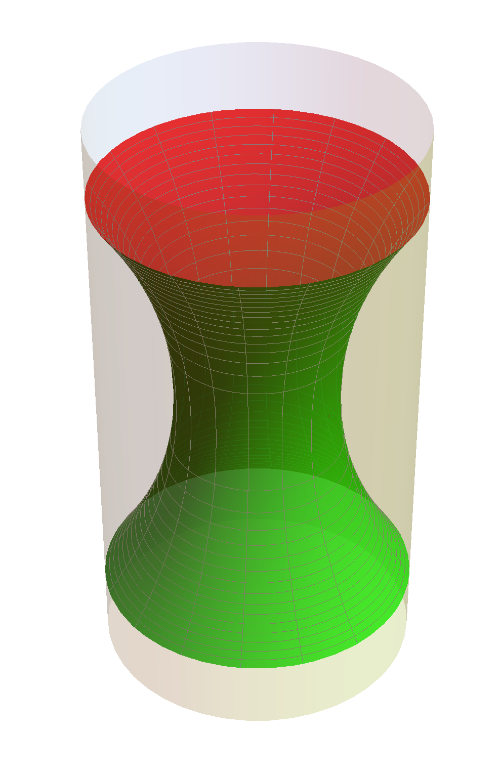
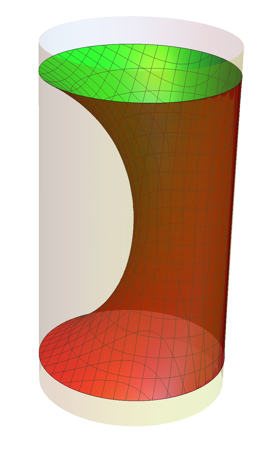
Figure 1. Vertical catenoid and parabolic generalized catenoid.

These surfaces, called catenoids, have the following properties:

1. $C_{h}$ is a bigraph with respect to the horizontal plane $\mathbb{H}^{2}\times\{0\}$.

2. As $h\searrow 0$, $C_{h}$ converges to $\mathbb{H}^{2}\times\{0\}$, branched at the origin, with multiplicity $2$.

3. As $h\nearrow\pi/2$, $C_{h}$ diverges to $\partial_{\infty}\mathbb{H}^{2}\times[-\pi/2,\pi/2]$.

Remark 2.1.

Let $T_{z_{0}}$ denote the horizontal dilation that maps $(0,t)$ into $(z_{0},t)\in\mathbb{H}^{2}\times\mathbb{R}$,

$$T_{z_{0}}(z,t):=\left(\frac{z+z_{0}}{\overline{z_{0}}z+1},t\right),$$

and define $C_{h,z_{0}}:=T_{z_{0}}(C_{h})$. When $z_{0}$ is the origin we simply write $C_{h}$. Then the family ${\mathcal{M}}:=\{C_{h,z_{0}}\;:\;(z_{0},h)\in\mathbb{H}^{2}\times\mathbb{R}\}$ forms a $3$-dimensional submanifold of the Banach manifold of all annuli.

2.2. Parabolic generalized catenoids.

Although $C_{h}$ diverges as $h\to\pi/2$, one can obtain a nontrivial limit of this family as follows. For each $h$ apply a hyperbolic isometry $T_{h}$ of $\mathbb{H}^{2}$, acting trivially on the $\mathbb{R}$ factor, which translates along a fixed geodesic passing through the origin and ending at a point $q$ in $\partial_{\infty}\mathbb{H}^{2}$. We fix $T_{h}$ completely by demanding that $o\in T_{h}(C_{h})$; the tangent plane at that point is then necessarily vertical. There exists a nontrivial limit ${\mathcal{D}}={\mathcal{D}}_{q}$ of the $T_{h}(C_{h})$, as $h\to\pi/2$, discovered originally by Hauswirth [5] and Daniel [4]. Its asymptotic boundary consists of the two circles $\mathbb{S}^{1}\times\{\pm\pi/2\}$ together with a vertical segment $\{q\}\times[-\pi/2,\pi/2]$. It is foliated by horocycles $H_{t}={\mathcal{D}}\cap(\mathbb{H}^{2}\times\{t\})$ based at the point $(q,t)$. Note that applying other horizontal dilations along the same geodesic produces a family of minimal surfaces with the same asymptotic boundary which foliate the slab $\mathbb{H}^{2}\times(-\pi/2,\pi/2)$; one limit of this family is the two disks $\mathbb{H}^{2}\times\{\pm\pi/2\}$. We shall refer them as parabolic generalized catenoids.

These families of surfaces enjoy the following uniqueness properties:

1. (Nelli, Sa Earp & Toubiana [15]): A minimal annulus bounded by $(\mathbb{S}^{1}\times\{\pm h\})$, for any $h\in(0,\pi/2)$, must equal $C_{h,z_{0}}$ for some $z_{0}\in\mathbb{H}^{2}$.

2. (Daniel, Hauswirth [4, 5]): If $X$ is any (possibly incomplete) minimal surface in $\mathbb{H}^{2}\times\mathbb{R}$, the intersection of which with any horizontal plane $\mathbb{H}^{2}\times\{t\}$ is a piece of a horocycle, then it must be a piece of some parabolic generalized catenoid.

These are interesting model examples and provide very useful barriers.

2.3. The Jacobi operator

We now derive an explicit expression for the Jacobi operator $L$ on a catenoid $C$ and determine the space of decaying Jacobi fields.

We first recall the Jacobi operator

$$L_{C}=\Delta_{C}+|S_{C}|^{2}+\mathrm{Ric}(\nu,\nu),$$

where $S_{C}$ is the shape operator (or second fundamental form) of $C$ and $\nu$ is the unit normal vector field to $C$. Rather than computing the last two terms explicitly, we use the coordinates and explicit form of the metric above to note that

$$L_{C}=\frac{(1-r^{2})^{2}}{4r^{2}}(\kappa^{-2}\partial_{t}^{2}+\partial_{\theta}^{2}+q(t)),$$

for some function $q$, where $\kappa$ is the parameter given by (2.1). We can determine $q$ by plugging in a known solution of $L_{C}w=0$, and we shall use the Jacobi field $w$ arising from vertical translations.

To calculate this Jacobi field, we first compute the unit normal to $C$,

$$\nu=\left(\frac{(1-r^{2})^{2}}{4\kappa r}\cos\theta,\frac{(1-r^{2})^{2}}{4\kappa r}\sin\theta,-\frac{r^{\prime}}{\kappa r}\right).$$

The Killing field generated by vertical translation is $(0,0,1)$, hence its projection onto $\nu$ is simply $-1/\kappa$ times the function $r^{\prime}/r$. In other words, $L_{C}(r^{\prime}/r)=0$. A short calculation then gives that

$$q=\frac{1}{2\kappa^{2}}(r^{-2}+r^{2}),$$

so altogether,

(2.2) $$L_{C}=\frac{(1-r^{2})^{2}}{4\kappa^{2}r^{2}}\left(\partial_{t}^{2}+\kappa^{2}\partial_{\theta}^{2}+\frac{1}{2}(\frac{1}{r^{2}}+r^{2})\right).$$

Now set

$$\mathfrak{J}(C)=\{\psi\in L^{\infty}(C):L_{C}\psi=0\},\qquad\mathfrak{J}^{0}(C)=\mathfrak{J}(C)\cap L^{2}(C);$$

we shall actually consider only the subclass of Jacobi fields which extend to be ${\mathcal{C}}^{2,\alpha}$ on $\overline{C}$, but this will be discussed in detail in §6, along with many further properties of the Jacobi operator, both at $C$ and at any other $A\in\mbox{\gothfamily A}$. The space $\mathfrak{J}(C)$ is infinite dimensional and is (almost) parametrized by its asymptotic boundary values. We note one special fact that if $\phi\in\mathfrak{J}^{0}(C)$, then $\phi$ is automatically smooth up to $\partial C$ as a function of $(r,\theta)$, and the $L^{2}$ condition means that it vanishes like $1-r$.

Expanding any function $u$ on $C$ as

$$u(t,\theta)=\sum_{n=0}^{\infty}(\alpha_{n}(t)\cos(n\theta)+\beta_{n}(t)\sin(n\theta)),\qquad\qquad(\mbox{with}\ \beta_{0}\equiv 0),$$

then

$$L_{C}u=\sum_{n=0}^{\infty}((L_{n}\alpha_{n})\cos(n\theta)+(L_{n}\beta_{n})\sin(n\theta)),$$

where

$$L_{n}=\frac{(1-r^{2})^{2}}{4\kappa^{2}r^{2}}\left(\partial_{t}^{2}-\kappa^{2}n^{2}+\frac{1}{2}(\frac{1}{r^{2}}+r^{2})\right).$$

Proposition 2.2.

The space of decaying Jacobi fields $\mathfrak{J}^{0}(C_{h})$ is spanned by $\varphi_{1}=\phi(r)\cos\theta$ and $\varphi_{2}=\phi(r)\sin\theta$, where

$$\phi(r):=\frac{1}{r}-r.$$

These are the Jacobi fields generated by horizontal dilations.

Proof.

We must determine all solutions to $L_{n}u=0$ with $u(\pm h)=0$. First observe that $L_{1}\phi=0$ where $\phi$ is given in the statement of the theorem. The Sturm-Picone comparison theorem then gives that any solution of the Dirichlet problem for $L_{n}$, $n\geq 1$, must be proportional to $\phi$, which is impossible for $n\geq 2$.

There is at most a two dimensional space of solutions to $L_{0}u=0$, and a basis for this space is given by the Jacobi fields generated by vertical translations and by varying the parameter $h$. We have already computed the first of these, which is the function $r^{\prime}/r$, which does not vanish at $\pm h$. It is easy to see that the second one cannot vanish at $\pm h$ either. ∎

3. Graphical parametrization of horizontal ends

In this section we extend and sharpen a result of Collin, Hauswirth and Rosenberg [1] and prove that any properly Alexandrov-embedded minimal annulus $A$ with embedded ends can be written as a vertical graph near infinity.

One key tool in the argument below is the family of ‘tall rectangles’ obtained in [4, 5, 17] (see also [10, 18]), which we now recall. Let $\sigma$ be any connected arc in $\mathbb{S}^{1}=\partial_{\infty}\mathbb{H}^{2}$ and denote by $\eta$ the geodesic in $\mathbb{H}^{2}$ with the same endpoints as $\sigma$. Also fix $a,b\in\mathbb{R}$ with $b-a>\pi$. Then there is a minimal disk $R(\sigma,a,b)$ with asymptotic boundary the rectangle $(\sigma\times\{a,b\})\cup(\partial\sigma\times[a,b])$, and such that for any $t_{0}\in(a,b)$, the projection onto $\mathbb{H}^{2}$ of the intersection $R(\sigma,a,b)\cap(\mathbb{H}^{2}\times\{t_{0}\})$ is a curve equidistant from the geodesic $\eta$. Furthermore, $R(\sigma,a,b)$ is symmetric with respect to the horizontal slice at height $(a+b)/2$, and is a vertical bigraph. If we denote by $\eta_{0}$ the projection of this central slice, all other horizontal slices project to curves ‘outside’ $\eta_{0}$, i.e., in the component of $\mathbb{H}^{2}\setminus\eta_{0}$ not containing $\eta$. The distance between $\eta$ and $\eta_{0}$ tends to $0$ as $b-a\nearrow\infty$ so it makes sense to define $R(\sigma,-\infty,\infty)$ to be the vertical plane $\eta\times\mathbb{R}$; $R(\sigma,-\infty,b)$ and $R(\sigma,a,\infty)$ to be the vertical graphs over the domain bounded by $\eta\cup\sigma$ with the corresponding boundary values, called ‘semi-infinite tall rectangles’. The distance from the central slice $\eta_{0}$ to $\eta$ tends to infinity as $b-a\searrow\pi$, and in fact if we simultaneously let $\sigma$ converges to the entire circle and $b-a\searrow\pi$ then $R(\sigma,a,b)$ converges to a parabolic generalized catenoid, which is foliated by horocycles (see Section 2.2).

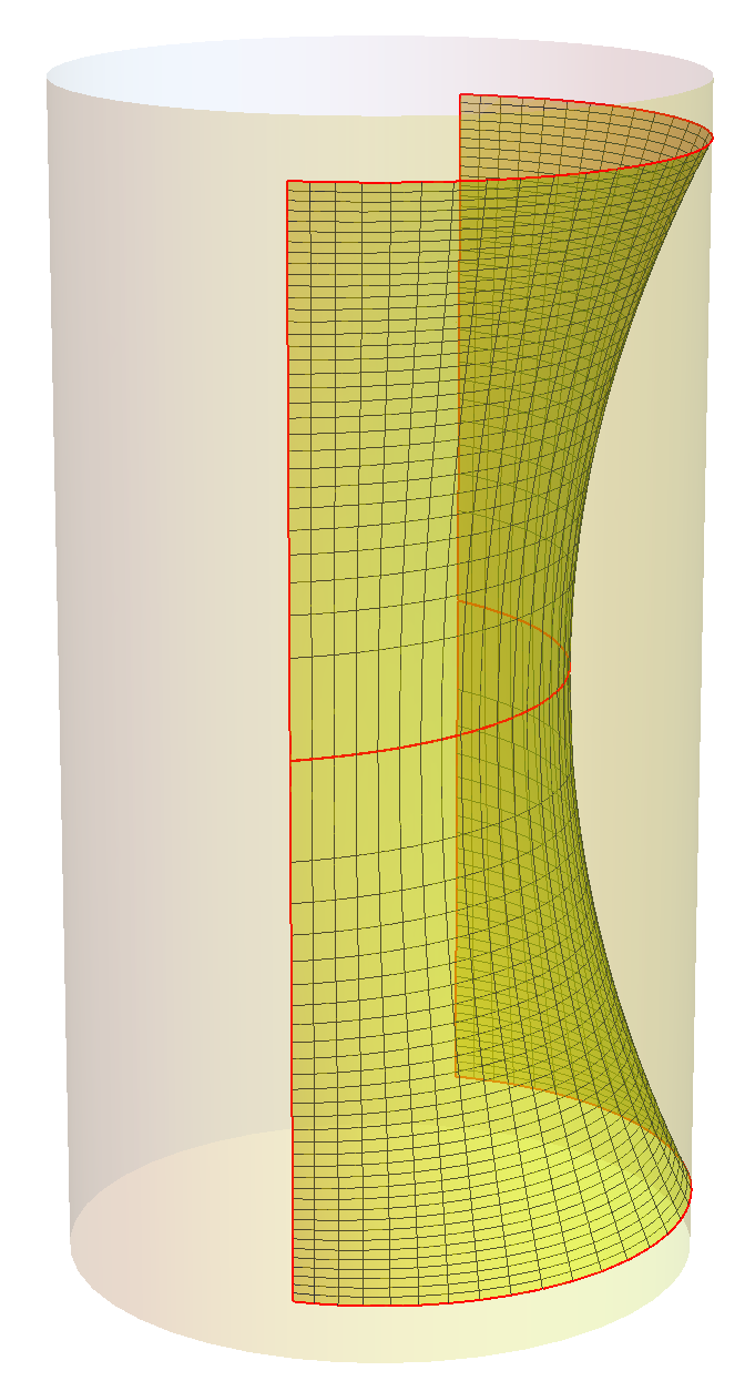
Figure 2. The tall rectangle for $\sigma$ equals to half the circumference at infinity and $b-a=\frac{9}{5}\pi$.

The other tool in this proof is the so-called ‘Dragging Lemma’ (which we state in a slightly simplified version adapted to our purposes), inspired in Colding and Minicozzi ideas.

Lemma 3.1 ([1]).

Let $E$ be a properly embedded annular end in $\mathbb{H}^{2}\times\mathbb{R}$ so that one component of its boundary, $\partial_{\operatorname{int}}E$, is a closed loop in the interior of this space and its virtual boundary at infinity, $\partial_{\infty}E=\gamma$, is a vertical graph of a continuous function $\gamma(\theta)$ over $\partial_{\infty}\mathbb{H}^{2}$. Suppose that $Y_{s}$ is a one-parameter family of compact minimal surfaces with boundary in $\mathbb{H}^{2}\times\mathbb{R}$ such that $Y_{s}\cap\partial E=\varnothing$ and $\partial Y_{s}\cap E=\varnothing$ for each $s\in[0,1]$. Suppose that $p_{0}\in Y_{0}\cap E$. Then there exists a continuous curve $s\mapsto p_{s}$ such that $p_{s}\in E\cap Y_{s}$ for each $s$ which equals $p_{0}$ at $s=0$.

We now turn to the main result of this section:

Proposition 3.2.

Let $E$ be a properly embedded annular end as in the previous lemma. Then for a sufficiently large $R>0$, there exists a function $u:\overline{\mathbb{H}^{2}}\setminus D_{\mathbb{H}^{2}}(o,R)\to\mathbb{R}$ with $u(1,\theta)=\gamma(\theta)$ such that the graph of $u$ equals $E\cap((\overline{\mathbb{H}^{2}}\setminus D_{\mathbb{H}^{2}}(o,R))\times\mathbb{R})$.

Remark 3.3.

The graph function $u$ is smooth in the interior and as regular at $\partial_{\infty}E$ as the function $\gamma(\theta)$, see the proof of Theorem 6.1 in Section §6.

Proof.

In the following we fix Euclidean coordinates $z=re^{i\theta}$ on $\overline{\mathbb{H}^{2}}$, and when we refer to the length of an arc on $\partial_{\infty}\mathbb{H}^{2}$, we mean with respect to the Euclidean metric and these coordinates.

For each $\epsilon>0$, there exists $\delta>0$ so that if $\sigma$ is an arc in $\mathbb{S}^{1}$ of length less than $\delta$, then $\mathrm{osc}_{\sigma}\gamma\ (=\sup_{\sigma}\gamma-\inf_{\sigma}\gamma)<\epsilon$. If the length of $\sigma$ is sufficiently small, then the semi-infinite tall rectangles $R(\sigma,-\infty,\inf_{\sigma}\gamma)$ and $R(\sigma,\sup_{\sigma}\gamma,\infty)$ do not intersect $\partial_{\operatorname{int}}E$, and by the maximum principle, neither of these intersect $E$ in its interior.

Fixing $\epsilon>0$ and a large constant $C_{1}<\frac{\pi}{4\epsilon}$, there exists a curve $\tilde{\eta}$ equidistant from the geodesic $\eta$ associated to $\sigma$ so that in the lens-shaped region $D_{\sigma}$ between $\sigma$ and $\tilde{\eta}$ the vertical distance between these upper and lower semi-infinite tall rectangles is less than $C_{1}\epsilon$ (see Fig. 3.) We then cover $\mathbb{S}^{1}$ by finitely many such arcs $\sigma$; the union of the corresponding lenses $D_{\sigma}$ covers an outer annular region $\mathbb{H}^{2}\setminus D_{\mathbb{H}^{2}}(o,R_{0})$, and in this region, the difference between the maximum and minimum height of $E\cap(\{p\}\times\mathbb{R})$ is less than $C_{1}\epsilon$. Clearly $E\cap((\mathbb{H}^{2}\setminus D_{\mathbb{H}^{2}}(o,R_{0}))\times\mathbb{R})$ is trapped in the region between the union of the upper and of the lower semi-infinite tall rectangles.

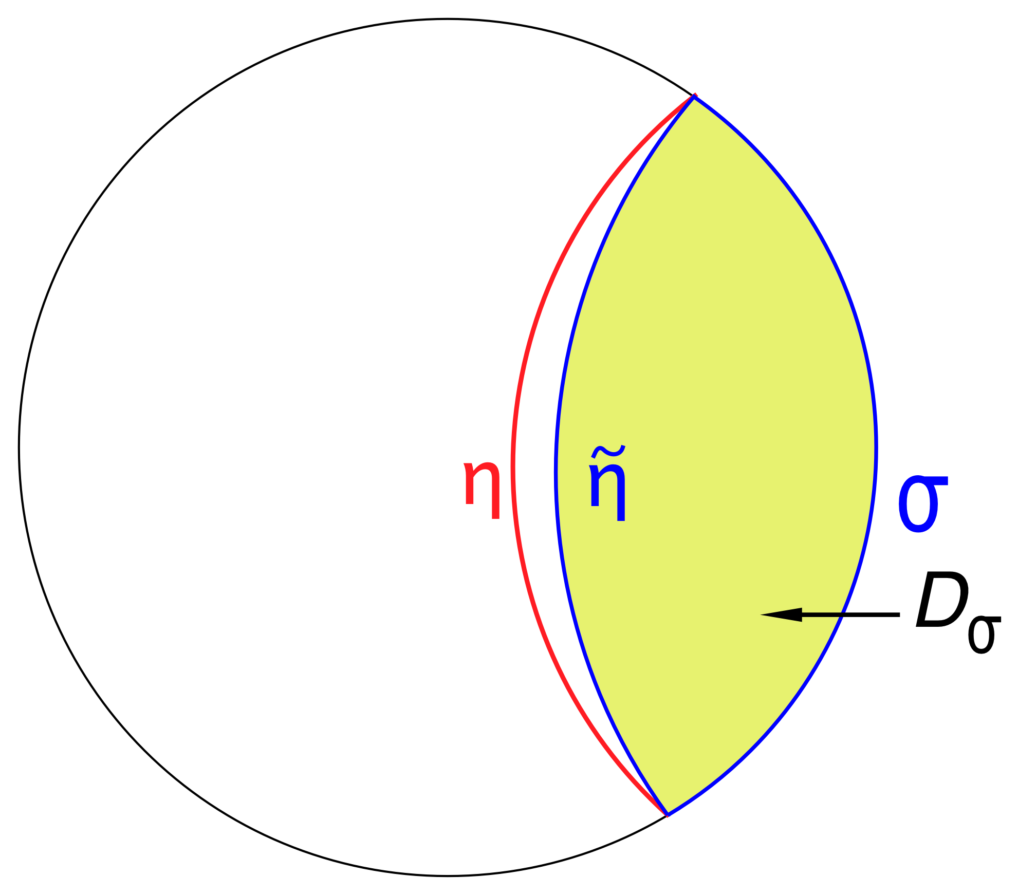
Figure 3. The region $D_{\sigma}$.

Next fix a truncated vertical catenoid $C$, i.e., the intersection of the catenoid centered on the axis $\{o\}\times\mathbb{R}$ of height $4C_{1}\epsilon$ with the cylinder $D_{\mathbb{H}^{2}}(o,\rho)\times\mathbb{R}$. We choose $\rho$ sufficiently large so that the vertical separation between the upper and lower boundaries of $C$ is greater than $3C_{1}\epsilon$. Denote by $C(q,\tau)$ the translate of this truncated catenoid by isometries of $\mathbb{H}^{2}\times\mathbb{R}$ so that it is centered at $(q,\tau)\in\mathbb{H}^{2}\times\mathbb{R}$. By the construction above, we may choose a radius $R_{1}\gg R_{0}$ so that $\partial_{\operatorname{int}}E\subset D_{\mathbb{H}^{2}}(o,R_{1})\times\mathbb{R}$, and a continuous function $q\mapsto\tau(q)$, $q\in\mathbb{H}^{2}\setminus D_{\mathbb{H}^{2}}(o,R_{1})$, satisfying

(3.1) $$C(q,\tau(q))\cap\partial_{\operatorname{int}}E=\varnothing,\mbox{ and $\partial C(q,\tau(q))\cap E=\varnothing$}$$

for every $q$ in this exterior region $\mathbb{H}^{2}\setminus D_{\mathbb{H}^{2}}(o,R_{1})$.

Denote by $E_{R}:=E\cap(({\mathbb{H}^{2}}\setminus D_{\mathbb{H}^{2}}(o,R))\times\mathbb{R})$ the region in $E$ outside a large cylinder. To prove Proposition 3.2, we must verify the following two assertions for $R\gg R_{1}$:

1. the projection $E_{R}\to\mathbb{H}^{2}\setminus D_{\mathbb{H}^{2}}(o,R)$ is bijective and

2. there are no points $(q,t)\in E_{R}$ such that $T_{(q,t)}E$ is vertical.

First note that i) is a consequence of ii). Indeed, if the projection of $E_{R}$ does not contain a full neighborhood of infinity, then there exists a sequence of points $q_{j}\in\mathbb{H}^{2}$ which tend to infinity and which do not lie in this image. Because $E$ is properly embedded, its projection on $\mathbb{H}^{2}$ is closed, so for each $j$ there exists $\kappa_{j}>0$ such that $D_{\mathbb{H}^{2}}(q_{j},\kappa_{j})$ is also disjoint from this image. Next, by translating the center $q_{j}$ in the component of the complement of the image of the projection of $E$, we may arrange that $\partial D_{\mathbb{H}^{2}}(q_{j},\kappa_{j})\times\mathbb{R}$ is tangent to $E$ at some point, and clearly the tangent plane of $E$ must be vertical there. This proves the surjectivity of this projection. Furthermore, if ii) holds, then the projection is a covering map, and properness of the embedding prevents there from being more than one sheet. Hence it must be bijective, and therefore a diffeomorphism.

We therefore turn to assertion ii). Choose $R_{2}>R_{1}+2\rho$ and let $K_{0}=(\overline{D_{\mathbb{H}^{2}}(o,R_{2})}\times\mathbb{R})\cap E$ be the corresponding compact portion of $E$. Properness of $E$ guarantees that $K_{0}$ has a finite number of connected components and also that there exists a connected compact subset $K\subset E$ such that $K_{0}\subset K$. In particular, any two points in $K_{0}$ can be joined by a path contained in $K$.

Now suppose there exists a point $(q,t)\in E\setminus K$ such that $T_{(q,t)}E$ is the vertical plane $\widetilde{\eta}\times\mathbb{R}$, where $\widetilde{\eta}$ is a geodesic in $\mathbb{H}^{2}$. Transform the whole ensemble by an isometry $T$ carrying $\widetilde{\eta}$ to the geodesic $\eta=\{z\in\mathbb{H}^{2},\operatorname{Re}(z)=0\}$, with $T(q,t)=(o,0)$; we also write $T(o,0)=(q_{0},t_{0})$ for the image point, which lies in $\{z\in\mathbb{H}^{2},\operatorname{Re}(z)\geq 0\}\times\mathbb{R}$. Note that there exists $C_{2}>0$ so that $T(E)$ lies in the horizontal slab $\mathbb{H}^{2}\times[-C_{2},C_{2}]$.

Fix $\delta^{\prime}>0$ and consider the geodesic $\widehat{\eta}\subset\{z\in\mathbb{H}^{2},\operatorname{Re}(z)<0\}$ which is orthogonal to $\{\operatorname{Im}(z)=0\}$ and at hyperbolic distance $\delta^{\prime}$ from $\eta$ (thus $o$ is the closest point on $\eta$ to $\widehat{\eta}$). Also let $\widehat{\sigma}\subset\partial_{\infty}\mathbb{H}^{2}$ be the boundary arc connecting the endpoints of $\widehat{\eta}$ and containing the endpoints of $\eta$. We denote by $\widehat{\eta}(\delta^{\prime})$ the curve equidistant from $\widehat{\eta}$ at distance $\delta^{\prime}$ and on the same side of $\mathbb{H}^{2}\setminus\hat{\eta}$ as $\eta$ (see Fig. 4.) There is a unique tall rectangle $R(\hat{\sigma},-h^{\prime},h^{\prime})$ which meets $\mathbb{H}^{2}\times\{0\}$ at $\hat{\eta}(\delta^{\prime})$, and is tangent to $\eta\times\mathbb{R}$, and hence $T(E)$, at $(o,0)$. Note that $\delta^{\prime}$ and $h^{\prime}$ are determined by one another, and $h^{\prime}\to\infty$ as $\delta^{\prime}\to 0$.

Figure 4. The lunette region $\Omega$ between the core curve $\hat{\eta}(\delta^{\prime})=R(\hat{\sigma},-h^{\prime},h^{\prime})\cap\{t=0\}$ and the equidistant curve $\eta^{\prime}$, which is the projection to $\mathbb{H}^{2}$ of $R(\hat{\sigma},-h^{\prime},h^{\prime})\cap\{t=\pm 2C_{2}\}$.

Claim 3.4.

For $h^{\prime}$ and $\operatorname{dist}_{\mathbb{H}^{2}}(o,q_{0})(=\operatorname{dist}_{\mathbb{H}^{2}}(q,o))$ sufficiently large, $\mathcal{R}=R(\hat{\sigma},-h^{\prime},h^{\prime})$ does not intersect $T(K)$.

Indeed, suppose that $h^{\prime}>3C_{2}$ and $\eta^{\prime}$ be the curve equidistant from $\hat{\eta}$ which is the projection to $\mathbb{H}^{2}$ of $\mathcal{R}\cap\{t=\pm 2C_{2}\}$. Let $\Omega$ be the region between $\hat{\eta}(\delta^{\prime})$ and $\eta^{\prime}$ (see Fig. 4.) We know that $T(E)\cap\mathcal{R}\subset\Omega\times\mathbb{R}$, as $T(E)\subset\mathbb{H}^{2}\times[-C_{2},C_{2}]$. Furthermore, if $\operatorname{dist}_{\mathbb{H}^{2}}(o,q_{0})$ is large enough, $(\Omega\times\mathbb{R})\cap T(K)=\varnothing$, and Claim 3.4 follows.

Let $\mathcal{R}^{\pm}$ be the connected components of $(\mathbb{H}^{2}\times\mathbb{R})\setminus\mathcal{R}$, and assume that $T(K)\subset\mathcal{R}^{+}$. Locally around $(o,0)$, $T(E)\cap\mathcal{R}$ is the union of $n$ smooth curves meeting at equal angles. There are many foliations of $\mathbb{H}^{2}\times(-h^{\prime},h^{\prime})$ by families of tall rectangles of which $\mathcal{R}$ is one element. These may be used to sweep out either $\mathcal{R}^{\pm}\times(-h^{\prime},h^{\prime})$, and together with the maximum principle show that $T(E)\cap\mathcal{R}$ cannot bound a disk lying either in $\mathcal{R}^{+}$ or $\mathcal{R}^{-}$. In particular, $T(E)\cap\mathcal{R}^{+}$ has at least two distinct connected components $\Sigma_{1}$, $\Sigma_{2}$.

If $\lambda>0$ is arbitrary, denote by $\mathcal{R}(\lambda)\subset\mathcal{R}^{+}$ the hyperbolic translation of $\mathcal{R}$ along $\{\operatorname{Im}(z)=0\}$ by the distance $\lambda$. We also write $\mu=\mathcal{R}(\lambda)\cap(\mathbb{H}^{2}\times\{0\})$ and $\mathcal{R}(\lambda)^{+}$ for the connected component of $(\mathbb{H}^{2}\times\mathbb{R})\setminus\mathcal{R}(\lambda)$ in $\mathcal{R}^{+}$. When $\lambda$ is sufficiently small, $\mathcal{R}(\lambda)$ meets both of the $\Sigma_{j}$, and in addition, $T(K)\subset\mathcal{R}(\lambda)^{+}$.

Let $\mathcal{U}$ be a connected component of $\Sigma_{i}\cap\mathcal{R}(\lambda)^{+}$, $i=1$ or $2$. If $\overline{\mathcal{U}}$ is compact, then the same argument as above shows that the case where $\partial\mathcal{U}\subset\mathcal{R}(\lambda)$ is impossible. We thus turn to the remaining case $\partial_{\operatorname{int}}T(E)\subset\partial\mathcal{U}$. We can then consider a continuous path in $\mathcal{U}\subset T(E)\cap\mathcal{R}^{+}$ from a point $x_{i}\in\Sigma_{i}\cap\mathcal{R}(\lambda)$ to a point $y_{i}\in\partial_{\operatorname{int}}T(E)\subset T(K_{0})$.

Suppose now that $\overline{\mathcal{U}}$ is non-compact. We are also going to construct a continuous path in $T(E)\cap\mathcal{R}^{+}$ from a point $x_{i}\in\Sigma_{i}$ to a point in $y_{i}\in T(K_{0})$. Adjoining this to a continuous path in $T(K)$ connecting $y_{1}$ and $y_{2}$ gives a continuous path in $T(E)\cap\mathcal{R}^{+}$ between $x_{1}\in\Sigma_{1}$ and $x_{2}\in\Sigma_{2}$. This contradicts that $\Sigma_{1}$ and $\Sigma_{2}$ are different components of $E\cap\mathcal{R}^{+}$. Hence there would not exist a point $(q,t)\in E\setminus K$ whose tangent plane $T_{(q,t)}E$ is the vertical, if $\operatorname{dist}_{\mathbb{H}^{2}}(q,o)$ is large enough, and assertion ii) would follow. Then in order to complete the proof of assertion ii) is suffices to construct such a path in the case $\overline{\mathcal{U}}$ is non-compact.

Since $\overline{\mathcal{U}}$ is non-compact, there exist a point $x_{i}\in\Sigma_{i}\cap\mathcal{R}(\lambda)^{+}$ sufficiently far from both $\mathcal{R}$ and $T(D_{\mathbb{H}^{2}}(o,R_{1}))\times\mathbb{R}$ so that a truncated catenoid $C(\hat{x}_{i},\tau(\hat{x}_{i}))$ passes through $x_{i}$, for some point $\hat{x}_{i}\in\mathbb{H}^{2}\setminus T(D_{\mathbb{H}^{2}}(o,R_{1}))$. Let $\xi_{i}(s)$ be a curve in $\mathbb{H}^{2}\times\mathcal{R(\lambda)}^{+}$ joining $\hat{x}_{i}$ to a point in $T(D_{\mathbb{H}^{2}}(o,R_{1}+\rho))\times\mathbb{R})$. We can assume that $\xi_{i}$ is at a distance bigger than $2\rho$ from $\mathcal{R}$ at any point. From (3.1), the translated catenoids $C(\xi_{i}(s),\tau(\xi_{i}(s)))$ satisfy

$$C(\xi_{i}(s),\tau(\xi_{i}(s)))\cap\partial_{\operatorname{int}}T(E)=\varnothing\quad{\rm and}\quad\partial C(\xi_{i}(s),\tau(\xi_{i}(s)))\cap T(E)=\varnothing.$$

Lemma 3.1 shows that there exists a continuous curve $s\mapsto p_{s}$ such that $p_{s}\in E\cap C(\xi_{i}(s),\tau(\xi_{i}(s)))$ for each $s$. This gives a continuous path in $E\cap\mathcal{R}^{+}$ from a point $x_{i}$ in $\Sigma_{i}$ to a point $y_{i}\in T(K_{0})\subset T(K)$, as desired. ∎

Remark 3.5.

We observe that the graphical behaviour of the asymptotic boundary of the annulus has only been used to ensure the existence of truncated catenoids satisfying (3.1). This conclusion may also be obtained in the following setting where somewhat less is known. Consider two functions $\alpha^{\pm}\in{\mathcal{C}}^{2,\alpha}(\mathbb{S}^{1})$ such that $0<\alpha^{+}(\theta)-\alpha^{-}(\theta)<\pi$ for all $\theta\in\mathbb{S}^{1}$. Suppose also that $E$ is a properly embedded minimal annulus with one compact boundary component and $\partial_{\infty}E$ lies between the graphs of $\alpha^{\pm}$, i.e., $\partial_{\infty}E\subset\{(\theta,t)\in\mathbb{S}^{1}\times\mathbb{R}\;:\;\alpha^{-}(\theta)<t<\alpha^{+}(\theta)\}$. Then $E$ is graphical in some region $\{|z|>1-\epsilon\}$. In particular, necessarily $\partial_{\infty}E$ is a vertical graph.

If we remove the hypothesis of embeddedness in Proposition 3.2, then the assertion is not longer necessarily true. However, the proof above still shows that for small enough $\epsilon>0$, there is no point in $E\cap(\{|z|>1-\epsilon\}\times\mathbb{R})$ where the tangent plane to $E$ is vertical. This means that near infinity, $E$ is a multi-graph.

We conclude this section with a closely related result about the shape of the set of points on $A$ where the tangent plane is vertical.

Proposition 3.6.

Let $A$ be a properly Alexandrov-embedded, minimal annulus with embedded ends such that $\Pi(A)=(\gamma^{+},\gamma^{-})$ consists of two ${\mathcal{C}}^{2,\alpha}$ graphs over $\mathbb{S}^{1}$. Then the set $V$ of all points on $A$ where the tangent plane is vertical (or equivalently, where the normal has no vertical component) is a regular curve which generates $H_{1}(A,\mathbb{Z})$. Moreover, the Gauss map of $A$ restricted to $V$, $\nu|_{V}$, is a diffeomorphism from $V$ to the equator of the unit sphere $\mathbb{S}^{2}$.

Proof.

Suppose $H_{s}$ is a smooth ‘sweepout’ of $\mathbb{H}^{2}\times\mathbb{R}$ by vertical planes. In other words, the $H_{s}$ are leaves of a smooth foliation. Assuming that the parameter $s$ varies over $\mathbb{R}$, we define a height function $K:\mathbb{H}^{2}\times\mathbb{R}\to\mathbb{R}$ by setting $H_{s}=\{K=s\}$. Let $K_{A}$ denote the restriction of $K$ to $A$. We claim that $K_{A}$ is a Morse function with precisely two critical points, each of index $1$.

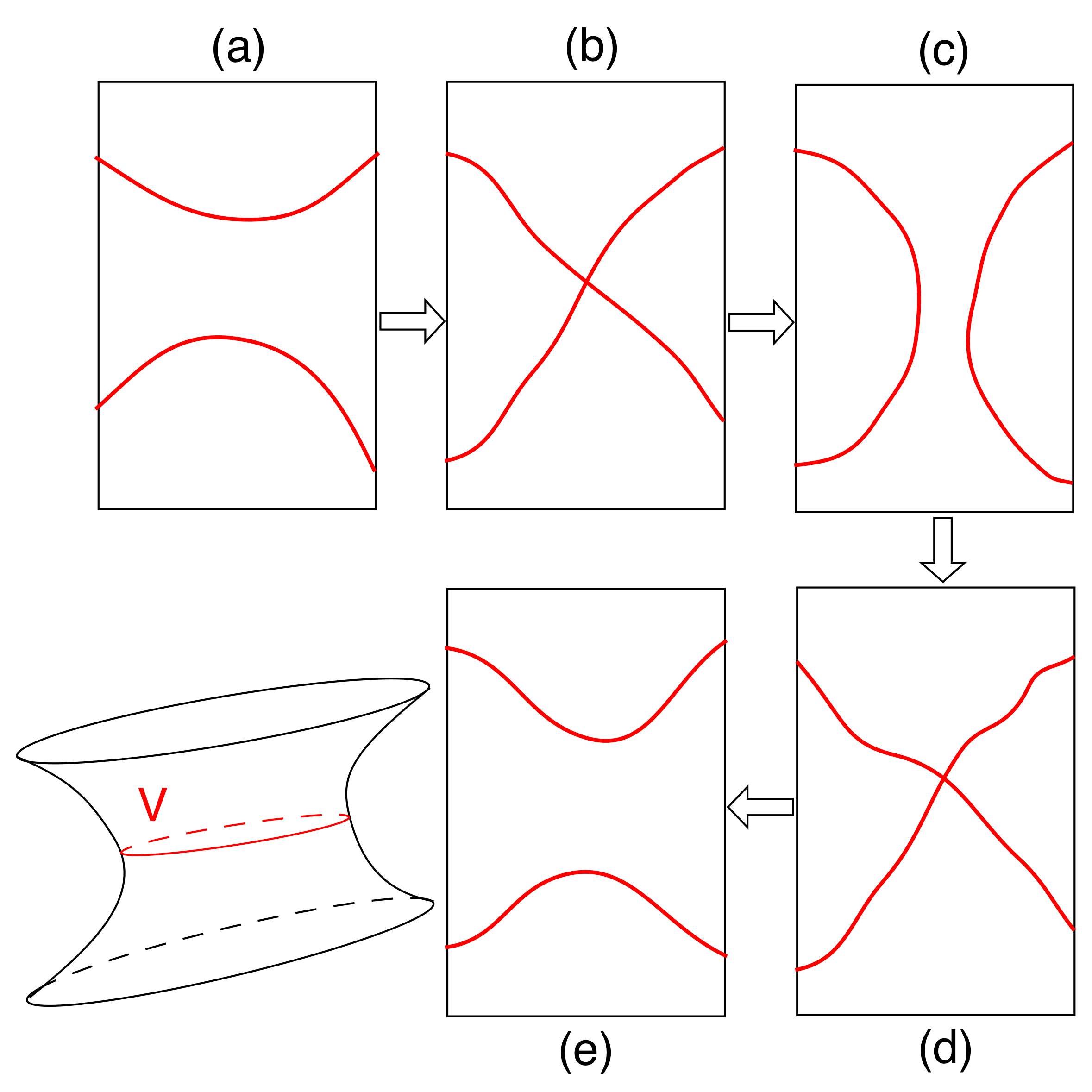
Figure 5. Evolution of $H_{s}\cap A$ when there are no loops.

The graphical representation theorem proved in this section shows that for $s$ very negative, $H_{s}\cap A$ is a union of two arcs, each one lying in an end of $A$. In fact, for any value of $s$, $H_{s}\cap A$ intersects a neighborhood of $\partial_{\infty}\mathbb{H}^{2}\times\mathbb{R}$ in four simple arcs, two arriving in $\gamma^{+}$ and two arriving in $\gamma^{-}$. Now as $s$ increases from $-\infty$ there is a point of first tangency with $A$, say at $s=s_{1}$, which occurs at a point $p_{1}\in V$. Locally around $p_{1}$, $H_{s_{1}}\cap A$ is a union of $\ell$ curves intersecting at equal angles for some $\ell\geq 2$.

If there is not any closed loop then the shape of $H_{s_{1}}\cap A$ is as in Figure 5-(b). In particular $\ell=2$. If there is $\sigma$ a closed loop in $H_{s_{1}}$, then (by the maximum principle) $\sigma$ cannot bound a compact disk in $A$. So $\sigma$ generates $H_{1}(A,\mathbb{Z})$. By the maximum principle again, there is only one such loop. In particular, $\ell\leq 3$. If $\ell=3$ then $\sigma$ separates $\gamma^{+}$ and $\gamma^{-}$ and so it separates the diverging arcs in $H_{s_{1}}\cap A$, two on each region of $H_{s_{1}}\setminus\sigma$. But this is absurd because one of the components of $H_{s_{1}}\setminus\sigma$ is compact. Hence $\ell=2$ and the shape of $H_{s_{1}}\cap A$ is either as in Figure 6-(b) or as in Figure 7-(c).

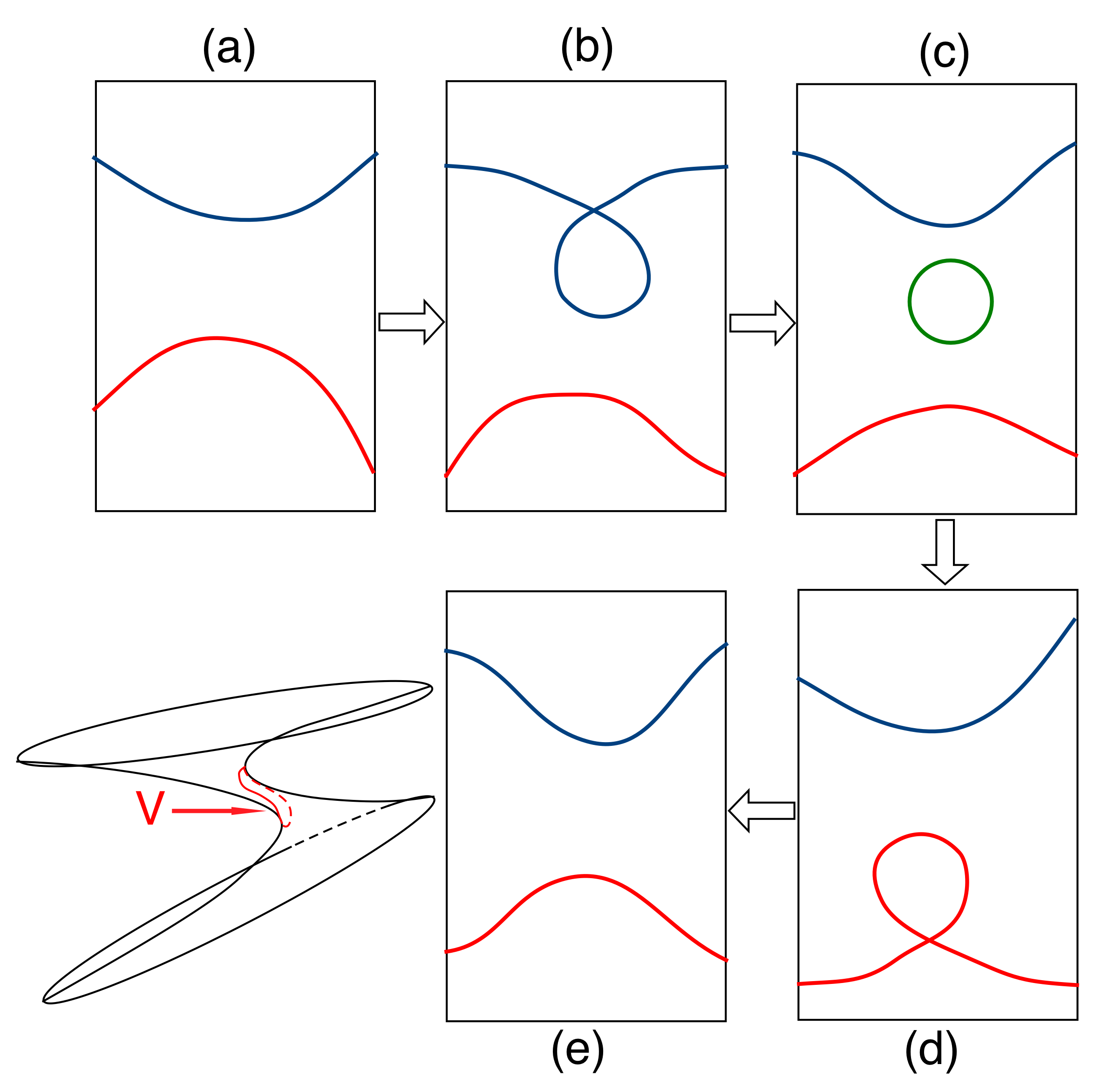
Figure 6. Possible evolution of $H_{s}\cap A$ and the curve $\sigma$, when $\sigma$ is a generator of $H_{1}(A,\mathbb{Z})$.

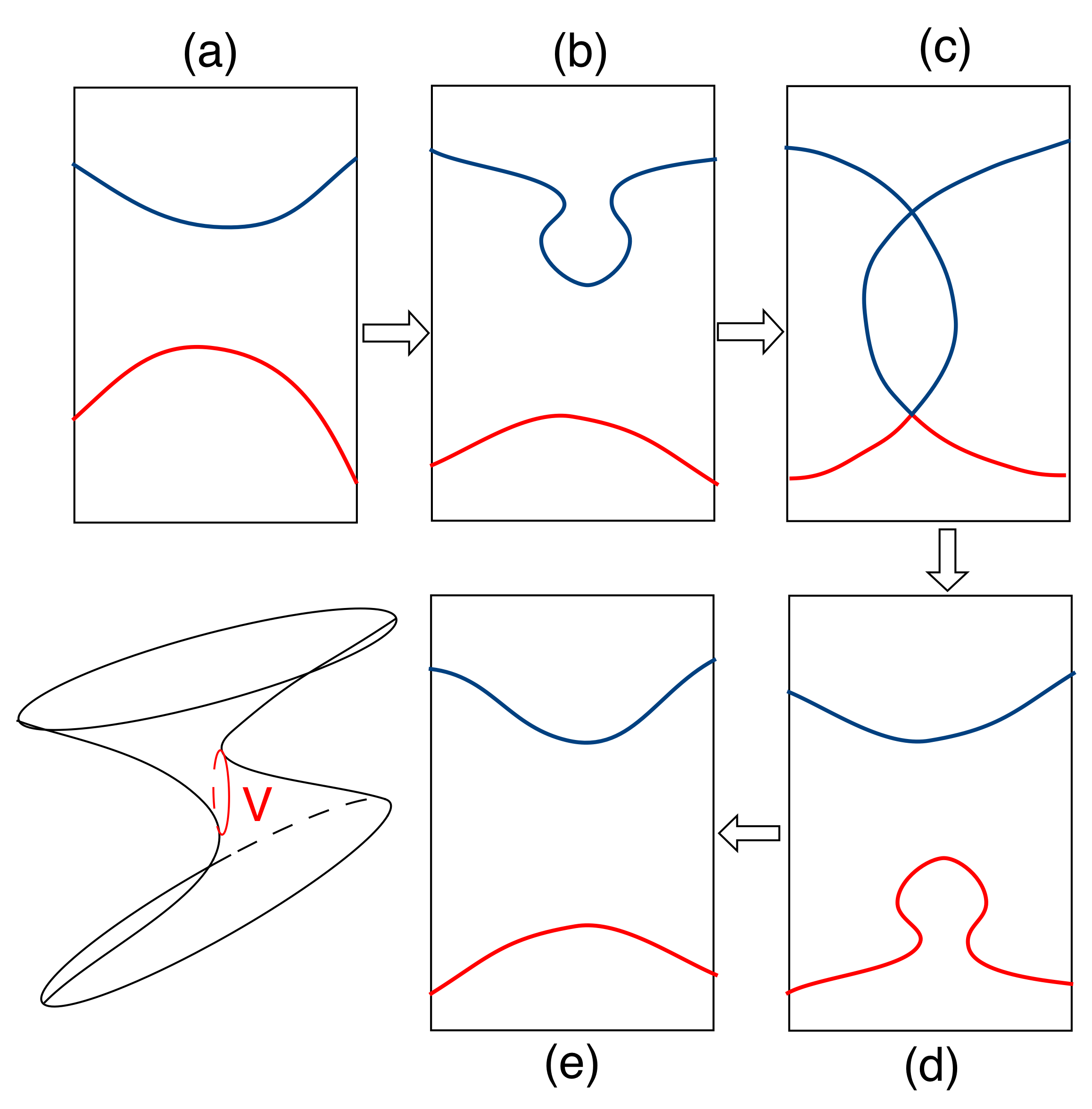
Figure 7. The other possible evolution of $H_{s}\cap A$ and the curve $\sigma$, when it contains a generator of $H_{1}(A,\mathbb{Z})$.

In any case $\ell=2$, and hence this is a simple tangency, or in other words, the function $K_{A}$ has a nondegenerate critical point of index $1$ at $s_{1}$. Letting $s$ increase further, we encounter some number of other critical points $p_{2},\ldots,p_{r}$, at the values $s=s_{2},\ldots,s_{r}$, each one of which corresponds to another nondegenerate critical point of index $1$ of $K_{A}$.

To conclude, observe that we can apply the standard Morse-theoretic arguments to see how these critical points correspond to a decomposition of $A$ into a union of cells.

In the first case (Figure 5), for $s$ very negative, $A\cap\{K_{A}\leq s\}$ is a union of two disks. The transition between the sublevel $K_{A}\leq s_{1}-\epsilon$ and $K_{A}\leq s_{1}+\epsilon$ corresponds to attaching a two-cell which connects these two disks, resulting in another (topological) disk. Crossing the next critical point, another two-cell is added, which changes the topology again. Each of the remaining critical points add further handles. However, since $A$ is an annulus, and in particular has genus $0$, we must have $r=2$. Hence there are precisely two critical points.

In the second case (Figure 6), again we have that for $s$ very negative, $A\cap\{K_{A}\leq s\}$ is a union of two disks. Now, the transition between the sublevel $K_{A}\leq s_{1}-\epsilon$ and $K_{A}\leq s_{1}+\epsilon$ corresponds to attaching a two-cell which connects one of the disks with itself, resulting in a topological annulus. Crossing the next critical point, another two-cell is added, which connects the annulus with the other disk. Again we deduce that $r=2$. Using similar arguments we deduce that $r=2$ in the last case (Figure 7).

Note that since both these critical points are nondegenerate, the set of points $p\in V$ near either $p_{1}$ or $p_{2}$ constitute a regular curve.

We may of course do this for any sweepout of $\mathbb{H}^{2}\times\mathbb{R}$ by vertical planes. This shows that in any direction, there are precisely two critical points and hence $V$ is a regular curve which generates $H_{1}(A,\mathbb{Z})$. ∎

4. Fluxes of minimal annuli

Let $A$ be a minimal surface lying in an ambient space which has continuous families of isometries, and $\gamma$ any closed curve in $A$. For any Killing field $Z$ on the ambient space, the flux of $A$ across $\gamma$, $\mbox{Flux}\,(A,\gamma,Z)$, depends only on the homology class of $\gamma$ in $A$. This flux is defined by integrating $\langle Z,\nu\rangle$ around $\gamma$, where $\nu$ is the unit normal to $\gamma$ in $A$. We now compute these flux integrals for minimal annuli in $\mathbb{H}^{2}\times\mathbb{R}$ with horizontal ends, where $\gamma$ is the generating loop for the homology $H^{1}(A,\mathbb{Z})$. These invariants play an important role later in this paper.

Fix $A\in\mbox{\gothfamily A}$, $\Gamma=(\gamma^{+},\gamma^{-})=\partial A$. As proved in §3 (Proposition 3.2 and Remark 3.3), each end of $A$ is a vertical graph over some region $\{z:R\leq|z|\leq 1\}$, with graph functions $u^{\pm}$, so we use the graphical representations

$$X^{\pm}(r,\theta)=(r\cos\theta,r\sin\theta,u^{\pm}(r,\theta)),\quad R\leq r\leq 1,\ \ \theta\in\mathbb{S}^{1}.$$

Consider the restriction of $X^{\pm}$ to $\beta^{\pm}:=X^{\pm}\cap\{r=\mathrm{const.}\}$ and the orthonormal frame

$$E_{1}=(\sqrt{F},0,0),\quad E_{2}=(0,\sqrt{F},0),\quad E_{3}=(0,0,1),$$

where $F=\frac{1}{4}(1-r^{2})^{2}$. Evaluating all functions at this fixed value of $r$,

$$\beta^{\pm}_{\theta}(\theta)=X_{\theta}^{\pm}(r,\theta)=-\frac{r\,\sin\theta}{\sqrt{F}}\,E_{1}+\frac{r\,\cos\theta}{\sqrt{F}}\,E_{2}+u^{\pm}_{\theta}\,E_{3},$$

hence the unit tangent to $\theta\mapsto\beta^{\pm}$ is

$$T^{\pm}(\theta)=\frac{\beta^{\pm}_{\theta}}{\|\beta_{\theta}^{\pm}\|_{g}},\quad\left\|\beta^{\pm}_{\theta}\right\|_{g}=\frac{\sqrt{r^{2}+F\,(u^{\pm}_{\theta})^{2}}}{\sqrt{F}}.$$

Similarly, the normal to this curve in $A$ equals

$$\nu^{\pm}(\theta)=\pm Q\left(\left(\frac{r\cos\theta}{\sqrt{F}}+\sqrt{F}u^{\pm}_{\theta}u^{\pm}_{x_{2}}\right)E_{1}+\left(\frac{r\sin\theta}{\sqrt{F}}-\sqrt{F}u^{\pm}_{\theta}u^{\pm}_{x_{1}}\right)E_{2}+ru^{\pm}_{r}E_{3}\right),$$

where $Q=\left(\|\beta^{\pm}_{\theta}\|_{g}\sqrt{1+F\|\nabla u^{\pm}\|^{2}}\right)^{-1}.$

We now compute the fluxes with respect to $E_{3}$ and the horizontal Killing fields generated by rotations and hyperbolic dilations.

The first is the simplest:

$$\text{ Flux}(A,\beta^{\pm},E_{3})=\int_{\beta^{\pm}}\langle\nu^{\pm},E_{3}\rangle\,d\sigma=\\ \pm\int_{0}^{2\pi}\frac{ru^{\pm}_{r}}{\sqrt{1+F\|\nabla u^{\pm}\|^{2}}}\,d\theta=\pm\int_{0}^{2\pi}\frac{ru^{\pm}_{r}}{\sqrt{1+\frac{1}{4}(1-r^{2})^{2}\left((u^{\pm}_{r})^{2}+r^{-2}(u^{\pm}_{\theta})^{2}\right)}}\,d\theta.$$

This is constant in $r$, and the limit as $r\nearrow 1$ equals

$$\text{ Flux}(A,\gamma^{\pm},E_{3})=\pm\int_{0}^{2\pi}u^{\pm}_{r}(1,\theta)\,d\theta.$$

Next, the Killing field generated by rotations around the vertical axis $\{0\}\times\mathbb{R}$ is

$$Z=-\frac{r\sin\theta}{\sqrt{F}}\,E_{1}+\frac{r\cos\theta}{\sqrt{F}}\,E_{2},$$

and we have

$$\text{ Flux}(A,\beta^{\pm},Z)=\mp\int_{0}^{2\pi}\frac{r\,u^{\pm}_{\theta}\,u^{\pm}_{r}}{\sqrt{1+F\|\nabla u^{\pm}\|^{2}}}\,d\theta.$$

Letting $r\nearrow 1$ as before gives that

(4.1) $$\text{ Flux}(A,\gamma^{\pm},Z)=\mp\int_{0}^{2\pi}u^{\pm}_{r}(1,\theta)\;u^{\pm}_{\theta}(1,\theta)\,d\theta.$$

Finally, consider the Killing fields

$$H_{a}=\frac{r^{2}\cos(a-2\theta)-\cos(a)}{2\sqrt{F}}\,E_{1}-\frac{r^{2}\sin(a-2\theta)+\sin(a)}{2\sqrt{F}}\,E_{2},$$

$a\in[0,2\pi)$, corresponding to the horizontal dilations along the geodesic joining $\text{e}^{{\rm i}a}$ and $-1$. We calculate

$$\text{ Flux}(A,\beta^{\pm},H_{a})=\int_{\beta^{\pm}}\langle\nu^{\pm},H_{a}\rangle d\sigma\\ \ =\pm\int_{0}^{2\pi}\frac{1}{2\sqrt{1+F\|\nabla u^{\pm}\|^{2}}}\left(\left(\frac{4r}{r^{2}-1}+\frac{(r^{2}-1)(u^{\pm}_{\theta})^{2}}{r}\right)\cos(a-\theta)\right.\\ +(r^{2}+1)u^{\pm}_{r}u^{\pm}_{\theta}\sin(a-\theta)\bigg{)}\,d\theta.$$

Unlike the previous cases we cannot take limits directly since the first term appears to diverge. However,

$$\frac{1}{2\sqrt{1+F\|\nabla u^{\pm}\|^{2}}}\left(\frac{4r}{r^{2}-1}+\frac{(r^{2}-1)(u^{\pm}_{\theta})^{2}}{r}\right)=\frac{1}{r-1}+\frac{1}{2}+{\mathcal{O}}(1-r).$$

When we multiply by $\cos(\theta-a)$ and integrate in $\theta$, the first two terms on the right vanish, while the third vanishes in the limit as $r\nearrow 1$. Therefore only the final term remains and we obtain that

$$\text{ Flux}(A,\gamma^{\pm},H_{a})=\pm\int_{0}^{2\pi}u^{\pm}_{r}(1,\theta)\;u^{\pm}_{\theta}(1,\theta)\sin(\theta-a)\,d\theta.$$

These computations prove the following

Lemma 4.1.

Let $A$ be a complete properly embedded minimal annulus with horizontal ends, parametrized as above. Then

(4.2) $$\int_{0}^{2\pi}u^{+}_{r}(1,\theta)d\theta+\int_{0}^{2\pi}u^{-}_{r}(1,\theta)d\theta=0,$$

(4.3) $$\int_{0}^{2\pi}u^{+}_{r}(1,\theta)\;u^{+}_{\theta}(1,\theta)\,d\theta+\int_{0}^{2\pi}u^{-}_{r}(1,\theta)\;u^{-}_{\theta}(1,\theta)\,d\theta=0,$$

and for every $a\in[0,2\pi)$,

(4.4) $$\int_{0}^{2\pi}u^{+}_{r}(1,\theta)u^{+}_{\theta}(1,\theta)\sin(\theta-a)\,d\theta+\int_{0}^{2\pi}u^{-}_{r}(1,\theta)u^{-}_{\theta}(1,\theta)\sin(\theta-a)\,d\theta=0,$$

5. Nonexistence

We present here two separate results which limit the types of pairs of curves which can arise as boundaries of minimal annuli. The first proof is based on a standard barrier argument and the second on Alexandrov reflection principle. Among other things, we are going to prove in this section that there are no properly embedded minimal surfaces with two consecutive horizontal annular ends when these ends are more than $\pi$ apart. Observe that if there exists a horizontal slab of height greater than $\pi$ separating the boundaries, then the result can be easily proved by using the maximum principle and the family of catenoids described in §2. However, the general case is more involved.

In order to prove this, we need to show that two tall rectangles of the same height with the vertical segments in common are not area-minimizing (see Appendix A.)

We would like to remind that we are denoting the finite boundary of a surface $\Sigma$ as $\partial_{\operatorname{int}}\Sigma$.

Theorem 5.1.

Consider two curves $\alpha^{+}$ and $\alpha^{-}$ in $\mathcal{C}^{2,\alpha}(\mathbb{S}^{1})$ satisfying that $\alpha^{+}(\theta)-\alpha^{-}(\theta)>\pi$, for all $\theta\in\mathbb{S}^{1}$, and $D^{+}$ and $D^{-}$ the minimal disks so that $\partial_{\infty}D^{\pm}=\alpha^{\pm}$, respectively. We label $\Omega(\alpha^{+},\alpha^{-})$ the domain in $\mathbb{H}^{2}\times\mathbb{R}$ bounded by $D^{+}$ and $D^{-}$. Then there is not a connected, properly embedded, minimal surface $\Sigma$ with boundary (possibly empty) satisfying:

1. $\Sigma$ intersects both connected components of $(\mathbb{H}^{2}\times\mathbb{R})-\Omega(\alpha^{+},\alpha^{-})$.

2. $(\partial_{\infty}\Sigma\cup\partial_{\operatorname{int}}\Sigma)\cap\overline{\Omega(\alpha^{+},\alpha^{-})}=\varnothing.$

Proof.

We proceed by contradiction, assume that there exists a connected surface $\Sigma$ verifying the hypotheses of the theorem.

Given an element $b\in[0,\pi]$, we label $\alpha^{\pm}_{b}:=\alpha^{\pm}|_{[e^{-{\rm i}b},e^{{\rm i}b}]}$ the corresponding arcs in $\alpha^{+}$ and $\alpha^{-}$, respectively, between $e^{-{\rm i}b}$ and $e^{{\rm i}b}$. Similarly, we define $s_{x}:=\{e^{{\rm i}x}\}\times[\alpha^{-}(e^{{\rm i}x}),\alpha^{+}(e^{{\rm i}x})].$ Then we consider in $\partial_{\infty}(\mathbb{H}^{2}\times\mathbb{R})$ the Jordan curve $\Gamma_{b}:=\alpha_{b}^{+}\cup\alpha_{b}^{-}\cup s_{b}\cup s_{-b}$. According to Coskunuzer’s results [2, Theorem 2.13], we know that there exists a complete, area-minimizing disk $\mathcal{T}_{b}$ which spans $\Gamma_{b}$.

Using the surface $\Sigma$ as a barrier, we can prove that there exists a limit of the family $\mathcal{T}_{b}$, as $b\to\pi$, which is different from $D^{+}\cup D^{-}$. Let $\mathcal{T}$ denote the limit of this family that is a properly embedded, area-minimizing disk whose ideal boundary consists of $\alpha^{+}\cup\alpha^{-}\cup s_{\pi}.$

As $\alpha^{+}(\theta)-\alpha^{-}(\theta)>\pi$, we can place two tall rectangles, $R$ and $R^{\prime}$, placed at both sides of $s_{\pi}$ and satisfying $R\cap\mathcal{T}=R^{\prime}\cap\mathcal{T}=\varnothing.$ If $R$ and $R^{\prime}$ are close enough, then we can move the rectangles toward $s_{\pi}$ until the boundaries of the three surfaces; $\mathcal{T}$, $R$ and $R^{\prime}$ touch along a common vertical segment. This implies that the angle in which $\mathcal{T}$ meets $\partial_{\infty}(\mathbb{H}^{2}\times\mathbb{R})$ is bigger than the angle in which $R$ and $R^{\prime}$ meets $\partial_{\infty}(\mathbb{H}^{2}\times\mathbb{R})$. In particular, $\mathcal{T}$ would not extend smoothly to $s_{\pi}$.

We consider $T_{n}:\mathbb{H}^{2}\times\mathbb{R}\to\mathbb{H}^{2}\times\mathbb{R}$ the horizontal dilation along the geodesic $\beta$ connecting $(-1,0)$ and $(1,0)$ by ratio $n\in\mathbb{N}$. Let us denote $\mathcal{E}_{n}:=T_{n}(\mathcal{T})$. As $\{\mathcal{E}_{n}\}_{n\in\mathbb{N}}$ is a sequence of area-minimizing surfaces, then there is a sub-sequential limit $\mathcal{E}_{0}$, which is not empty because the angle in which $\mathcal{T}$ meets $s_{\pi}$ is not zero. Moreover, from the method in which we have obtained $\mathcal{E}_{0}$ we know that:

• $\mathcal{E}_{0}$ is area-minimizing.

• $\mathcal{E}_{0}$ is foliated by equidistant curves in horizontal slices.

• $\partial_{\infty}(\mathcal{E}_{0})$ consists of two horizontal cycles at height $\alpha^{+}(-1)$ and $\alpha^{-}(-1)$, respectively, and two vertical segments: $s_{\pi}$ and $\{1\}\times[\alpha^{-}(-1),\alpha^{+}(-1)].$

Hence, using the characterization of minimal surfaces invariant under hyperbolic dilations (see [5, 18]), we deduce that $\mathcal{E}_{0}$ consists of two tall rectangles of height $\alpha^{+}(-1)-\alpha^{-}(-1)$ symmetric with respect the totally geodesic plane $\beta\times\mathbb{R}.$

But this contradicts Lemma A.1 in Appendix A, because $\mathcal{E}_{0}$ would be area-minimizing. This contradiction proves that it is impossible to construct a connected, properly embedded, minimal surfaces satisfying items i) and ii). ∎

As a consequence, we have the following corollary:

Corollary 5.2.

Let $\gamma^{+}$ and $\gamma^{-}$ be two curves in $\mathcal{C}^{2,\alpha}(\mathbb{S}^{1})$ satisfying $\gamma^{+}(\theta)-\gamma^{-}(\theta)>\pi$, $\forall\theta\in\mathbb{S}^{1}$. Then there is not any properly embedded minimal annulus $A$ in $\mathbb{H}^{2}\times\mathbb{R}$ with $\partial A=\gamma^{+}\cup\gamma^{-}$.

Proof.

We apply the previous theorem to the curves $\alpha^{+}:=\gamma^{+}-\varepsilon$ and $\alpha^{-}:=\gamma^{-}+\varepsilon$ for a small enough $\varepsilon>0$. ∎

Finally, as a consequence of the proof of Theorem 5.1 we have

Corollary 5.3.

Let $\gamma^{+}$ and $\gamma^{-}$ be two curves as in the previous corollary, and consider the vertical segment $s_{\theta}:=\{\theta\}\times[\gamma^{-}(\theta),\gamma^{+}(\theta)]$. Then there is not any properly embedded minimal surface $S$ in $\mathbb{H}^{2}\times\mathbb{R}$ with $\partial S=\gamma^{+}\cup\gamma^{-}\cup s_{\theta}$.

Remark 5.4.

Notice that in the process of proving Theorem 5.1 we have obtained that the limit of the family of disks $\{T_{b},\;\;b\in(0,\pi)\},$ as $b\to\pi$, is the union of the two disks $D^{+}$, $D^{-}$ and the vertical segment $s_{\pi}$.

Remark 5.5.

We would like to point out that Theorem 5.1 is more general than the corollaries that we are going to use in this paper. We are not imposing any restriction neither about the genus nor the number of ends. For instance it shows that there are no Costa-Hoffman-Meeks type surfaces (like the ones constructed by Morabito [13] and their possible perturbations) so that the vertical distance between two consecutive ends is more than $\pi$.

For the next result we impose a monotonicity condition on $\Gamma=(\gamma^{+},\gamma^{-})$, which we normalize by centering around $\theta=0,\pi$. Thus suppose that $\gamma^{+}$ is monotone decreasing on $[0,\pi]$ and monotone increasing on $[\pi,2\pi]$, while $\gamma^{-}$ is monotone increasing on $[0,\pi]$ and monotone decreasing on $[\pi,2\pi]$. In other words, the two curves are tilted away from each other. Notice that we allow non-strict monotonicity in each interval.

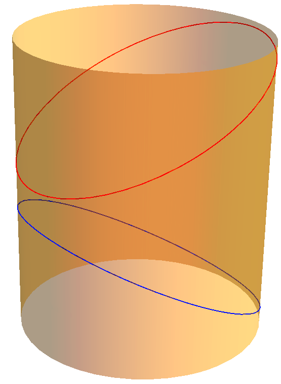
Figure 8. An example of curve $\Gamma$ in Proposition 5.6.

Proposition 5.6.

Under the conditions above, there is no $A\in\mbox{\gothfamily A}$ with $\partial_{\infty}A=\Gamma$ unless $\gamma^{\pm}$ are constant (in which case $A$ is a catenoid).

Proof.

Let $\eta(s)$ denote the geodesic in $\mathbb{H}^{2}$ which connects $(1,0)$ (where $\theta=0$) to $(-1,0)$, with $\eta(0)=(0,0)$ and $\eta\to(1,0)$ as $s\to-\infty$. For each $s$ denote by $\lambda_{s}$ the geodesic orthogonal to $\eta$ and meeting it at $\eta(s)$. The vertical plane $P_{s}=\lambda_{s}\times\mathbb{R}$ separates $\mathbb{H}^{2}\times\mathbb{R}$ into two components, ${\mathcal{U}}_{s}$ and ${\mathcal{V}}_{s}$, and we assume that $(1,0,0)\in\overline{{\mathcal{U}}_{s}}$.

Write $A_{s}^{\prime}=A\cap\overline{{\mathcal{U}}_{s}}$, $A_{s}^{\prime\prime}=A\cap\overline{{\mathcal{V}}_{s}}$, and denote by $A_{s}^{*}$ the reflection of $A_{s}^{\prime}$ into $\overline{{\mathcal{V}}_{s}}$. By Proposition 3.2, each end of $A$ is a vertical graph, $\mathbb{H}^{2}\setminus D(o,R)\ni z\mapsto(z,u^{\pm}(z))$. Then for $s\ll 0$, $A_{s}^{\prime}$ consists of two connected components, each of them a vertical graph. Since $u^{\pm}(1,\theta)=\gamma^{\pm}(\theta)$, the monotonicity hypotheses imply that the boundary curves $(\gamma_{s}^{*})^{\pm}$ of $A_{s}^{*}$ satisfy

$$(\gamma_{s}^{*})^{-}(\theta)\leq\gamma^{-}(\theta)<\gamma^{+}(\theta)\leq(\gamma_{s}^{*})^{+}(\theta)$$

for all $\theta$ with $e^{{\rm i}\theta}\times\mathbb{R}\subset\overline{{\mathcal{V}}_{s}}$. In addition, $\partial A_{s}^{*}\cap P_{s}=A\cap P_{s}$. By using the maximum principle with vertical translations of each connected component of $A_{s}^{*}$, we deduce that when $s$ is very negative, $A_{s}^{*}$ does not make contact with $A_{s}^{\prime\prime}$ except at the boundary. We then let $s$ increase until the first point of interior contact, which shows that $A_{s}^{*}=A_{s}^{\prime\prime}$ for some $s$. Therefore $\gamma^{\pm}$ are constant and $A$ is a rotationally invariant catenoid by [15, Theorem 2.1]. ∎

Remark 5.7.

The results of this section are still true if the annulus $A$ is Alexandrov-embedded with embedded ends.

6. The manifold of minimal annuli

In this section we prove the basic structural result about the space of minimal annuli.

Theorem 6.1.

The space $\mbox{\gothfamily A}^{\prime}$ of properly Alexandrov-embedded minimal annuli with embedded ends and ${\mathcal{C}}^{2,\alpha}$ boundary curves is a Banach submanifold in the space of complete properly immersed surfaces of class ${\mathcal{C}}^{2,\alpha}$ in $\mathbb{H}^{2}\times\mathbb{R}$.

Proof.

Fix any $A\in\mbox{\gothfamily A}^{\prime}$. We first note that $A$ is ${\mathcal{C}}^{2,\alpha}$ up to the boundary. Indeed, following [7], by the results of §3, there exists a neighborhood of infinity in $A$ which is the graph of a function $w:\mathbb{H}^{2}\setminus D_{\mathbb{H}^{2}}(o,R)\to\mathbb{R}$ for some $R\gg 1$, and this function extends (at least) continuously to $\partial\overline{\mathbb{H}^{2}}$. Near any point of the asymptotic boundary we may as well use the upper half-space representation of $\mathbb{H}^{2}$, and in such coordinates $(x,y)$ with $x\geq 0$, the minimal surface equation is

(6.1) $$w_{xx}(1+x^{2}w_{y}^{2})-2x^{2}w_{x}w_{y}w_{xy}+w_{yy}(1+x^{2}w_{x}^{2})-xw_{x}(w_{x}^{2}+w_{y}^{2})=0.$$

The remarkable and fortuitous fact is that although one might expect factors which are powers of $x$ coming from the corresponding factors in the hyperbolic metric in these coordinates, there is an overall factor of $x^{2}$ in this equation, so it becomes nondegenerate. In any case, from this expression it is standard that if the boundary at infinity is a ${\mathcal{C}}^{2,\alpha}$ graph, $\gamma=\gamma(y)$, then $w(x,y)$ is ${\mathcal{C}}^{2,\alpha}$ up to $x=0$.

The standard method is to parametrize surfaces ${\mathcal{C}}^{1}$ near to $A$ as normal graphs over $A$, i.e., as $\{\exp_{p}(u(p)\nu(p)):p\in A\}$, where $\nu$ is the unit normal vector field to $A$. It is more useful here, however, to alter this, replacing $\nu$ by a vector field $n$ for which $n=\nu$ in $A\cap(D_{\mathbb{H}^{2}}(o,R)\times\mathbb{R})$ and $n=\partial_{t}$ in $A\cap((\mathbb{H}^{2}\setminus D_{\mathbb{H}^{2}}(o,R^{\prime}))\times\mathbb{R})$ for some $R^{\prime}>R$. Thus, if $u$ is any small ${\mathcal{C}}^{2,\alpha}$ function, write

$$A_{u}=\{\exp_{p}(u(p)n(p)):p\in A\}.$$

The surface $A_{u}$ is minimal if $\mathcal{N}(u)=0$, where $\mathcal{N}$ is some degenerate second order quasilinear elliptic differential operator. Note that ${\mathcal{N}}$ is not the operator (6.1), but at least locally near $x=0$ of the form $x^{2}$ times that operator. In the ball model, let ${\mathcal{N}}=(1-r^{2})N$, so $N$ is a nondegenerate quasilinear elliptic operator. The linearization of ${\mathcal{N}}$ at $u=0$ is the Jacobi operator ${\mathcal{L}}$ relative to the vector field $n$. For normal graphs (i.e., using $\nu$ instead of $n$), this Jacobi operator is

$$\widehat{\mathcal{L}}\phi=(\Delta_{A}+|S|^{2}+\mbox{Ric}(\nu,\nu))\phi,$$

where $S$ is the shape operator (or second fundamental form) of $A$. With this slight change of parametrization, it is shown in [12][appendix] that

$${\mathcal{L}}=\widehat{{\mathcal{L}}}J,\quad J=n\cdot\nu.$$

Since $\nu=(-x^{2}w_{x},-x^{2}w_{y},1)/\sqrt{1+x^{2}(w_{x}^{2}+w_{y}^{2})}$, $J=1/\sqrt{1+x^{2}|\nabla w|^{2}}$, so $J$ is globally close to $1$, and moreover $J=1$ and $J_{x}=0$ at $x=0$.

We make one further reduction, noting that in the ball model, ${\mathcal{N}}$ is $(1-r^{2})$ times a nondegenerate operator, so its linearization can be divided by the same vanishing factor to obtain the linear modified Jacobi operator $L=(1-r^{2})^{-2}\widehat{{\mathcal{L}}}J$, which is simply the linearization of $N$, and this operator is now a standard nondegenerate elliptic operator. The net effect is that we can use standard elliptic theory (rather than the uniformly degenerate elliptic theory from [11] needed to study ${\mathcal{L}}$).

For a given $A\in\mbox{\gothfamily A}^{\prime}$, let us define

$$\mathfrak{J}(A)=\{\psi\in L^{\infty}(A):\widehat{\mathcal{L}}_{A}\psi=0\},\qquad\mathfrak{J}^{0}(A)=\mathfrak{J}(A)\cap L^{2}(A).$$

The main results about $N$ and $L$ are as follows.

Proposition 6.2.

Let $A\in\mbox{\gothfamily A}^{\prime}$ and suppose that $\partial A=\Gamma$ consists of a pair $\gamma^{\pm}$ of ${\mathcal{C}}^{2,\alpha}$ horizontal curves. Then

1. The graph function $u$ (relative to the parametrization using the vector field $n$) lies in ${\mathcal{C}}^{2,\alpha}(\overline{A})$;

2. If $\phi$ is a solution to $L\phi=0$ with boundary values $\phi_{0}^{\pm}\in{\mathcal{C}}^{2,\alpha}(\mathbb{S}^{1})$, then $\phi\in{\mathcal{C}}^{2,\alpha}(\overline{A})$;

3. The operator $L:{\mathcal{C}}^{2,\alpha}_{D}(A)\longrightarrow{\mathcal{C}}^{0,\alpha}(A)$ is Fredholm of index $0$, where ${\mathcal{C}}^{2,\alpha}_{D}$ is the space of ${\mathcal{C}}^{2,\alpha}$ functions which vanish at $\partial A$. Its kernel $\{\phi:L\phi=0\}$ is identified with $\mathfrak{J}^{0}(A)$ via $L\phi=0$ if and only if $\phi=J\varphi$, $\widehat{\mathcal{L}}\varphi=0$. (For simplicity, we often refer to this nullspace as $\mathfrak{J}^{0}(A)$, recalling this identification when appropriate.) This same finite dimensional space is a complement for its range;

4. If $\gamma^{\pm}\in{\mathcal{C}}^{\infty}$ and if $\phi\in\mathfrak{J}^{0}(A)$, i.e., $\phi_{0}^{\pm}=0$, then $\phi\in{\mathcal{C}}^{\infty}(\overline{A})$.

The only point that requires comment is the third; the fact that it is Fredholm is of course standard, and its index vanishes since it is deformable amongst elliptic Fredholm operators to a self-adjoint operator.

We say that $A$ is nondegenerate if $\mathfrak{J}^{0}(A)=\{0\}$. Define a continuous extension operator $e:{\mathcal{C}}^{2,\alpha}(\mathbb{S}^{1})^{2}\to{\mathcal{C}}^{2,\alpha}(A)$, and now consider the map

(6.2) $${\mathcal{C}}^{2,\alpha}(\mathbb{S}^{1})^{2}\times{\mathcal{C}}^{2,\alpha}_{D}(A)\ni((\phi_{0}^{+},\phi_{0}^{-}),w)\longrightarrow N(e(\phi_{0}^{+},\phi_{0}^{-})+w)\in{\mathcal{C}}^{0,\alpha}(A).$$

Proposition 6.3.

If $A\in\mbox{\gothfamily A}^{\prime}$ is nondegenerate, then there exists a neighborhood ${\mathcal{U}}$ of $0$ in ${\mathcal{C}}^{2,\alpha}(\mathbb{S}^{1})^{2}$ and a smooth map $G:{\mathcal{U}}\to{\mathcal{C}}^{2,\alpha}_{D}(A)$ such that $N(e(\phi_{0}^{+},\phi_{0}^{-})+G(\phi_{0}^{+},\phi_{0}^{-}))=0$, and all solutions $u$ to $N(u)=0$ sufficiently close to $0$ are of this form.

We reduce this to the implicit function theorem as follows. By hypothesis, the linearization of the map given by (6.2), $L$, is surjective, and there is a bijective correspondence between the nullspace of $L$ and pairs $\phi_{0}^{\pm}$. This last statement is a restatement of the fact that the linear Poisson problem is well-posed: there exists a unique homogeneous solution of $Lw=0$ with $w=\phi_{0}^{\pm}$ on $\gamma^{\pm}$.

To prove that $\mbox{\gothfamily A}^{\prime}$ is a Banach manifold even around degenerate annuli, we must characterize those pairs $(\phi^{+}_{0},\phi^{-}_{0})$ which occur as leading coefficients of elements of $\mathfrak{J}(A)$, which denotes the space of Jacobi fields of $A$. In the following, for $\phi\in\mathfrak{J}(A)$, we write $\phi_{1}$ for its normal derivative at the boundary (computed with respect to the fixed chart $z$).

Proposition 6.4.

Let $(\phi_{0}^{+},\phi_{0}^{-})$ be a pair of functions in $(\mathcal{C}^{2,\alpha}(\mathbb{S}^{1}))^{2}$. Then, there exists a Jacobi field $\phi\in\mathfrak{J}(A)$ satisfying $\phi|_{\partial A^{\pm}}=\phi_{0}^{\pm}$ if and only if

$$\int_{\mathbb{S}^{1}}(\phi^{+}_{0}\psi^{+}_{1}+\phi^{-}_{0}\psi^{-}_{1})=0$$

for every $\psi\in\mathfrak{J}^{0}(A).$

Proof.

First note that if $\widehat{\phi},\widehat{\psi}\in\mathfrak{J}^{0}(A)$, then

$$0 =\int_{A}(\widehat{\mathcal{L}}\widehat{\phi})\widehat{\psi}-\widehat{\phi}(\widehat{\mathcal{L}}\widehat{\psi})=\int_{\mathbb{S}^{1}}(\widehat{\phi}^{+}_{0}\widehat{\psi}^{+}_{1}-\widehat{\phi}^{+}_{1}\widehat{\psi}^{+}_{0})+(\widehat{\phi}^{-}_{0}\widehat{\psi}^{-}_{1}-\widehat{\phi}^{-}_{1}\widehat{\psi}^{-}_{0})$$

$$=\int_{\mathbb{S}^{1}}(\widehat{\phi}^{+}_{0}\widehat{\psi}^{+}_{1}+\widehat{\phi}^{-}_{0}\widehat{\psi}^{-}_{1}).$$

(The integrals at the two boundary components appear with the same sign because we are using the outward pointing normal derivative at each of these.) We may transfer this to an identify involving functions $\phi,\psi$ in the nullspace of $L$ by setting $\phi=J\widehat{\phi}$, $\psi=J\widehat{\psi}$ and also multiplying the area form of $A$ by $J^{-1}$; note also that $\phi_{0}^{\pm}=\widehat{\phi}^{\pm}_{0}$, $\psi_{0}^{\pm}=\widehat{\psi}_{0}^{\pm}$ because $J=1$ and its normal derivative vanishes at $\partial A$. Thus we also have

$$0=\int_{\mathbb{S}^{1}}(\phi^{+}_{0}\psi^{+}_{1}+\phi^{-}_{0}\psi^{-}_{1}).$$

In the following we perform the same integration by parts a few more times; each time we invoke the self-adjointness for $\widehat{\mathcal{L}}$ with respect to the geometric area form and then conjugate to obtain the analogous formula for the nondegenerate operator $L$ with respect to a new area form. However, for simplicity, we do not spell this out carefully again.

This necessary condition is also sufficient. Indeed, fix any $\phi_{0}^{\pm}$ satisfying this orthogonality condition, and set $u=e(\phi_{0}^{+},\phi_{0}^{-})$. Then $Lu=f\in{\mathcal{C}}^{0,\alpha}$. By part iii) of Proposition 6.2, there exists $\psi\in\mathfrak{J}^{0}(A)$ and $v\in{\mathcal{C}}^{2,\alpha}_{D}(A)$ such that $Lv=f+\psi$. Thus writing $\phi=v-u$, then $L\phi=\psi$. We now show that this is impossible unless $\psi=0$. Indeed, since $v$ vanishes at $\partial A$, $u^{\pm}=\phi_{0}^{\pm}$. Now we compute that

(6.3) $$\int_{A}|\psi|^{2}=\int_{A}(L\phi)\psi-\phi(L\psi)=\int_{\partial_{+}A}\phi_{0}^{+}\psi_{1}^{+}+\int_{\partial_{-}A}\phi_{0}^{-}\psi_{1}^{-}=0,$$

hence $\psi=0$. This completes the proof. ∎

This result proves that the set of pairs $(\phi^{+}_{0},\phi^{-}_{0})$ which can occur as leading coefficients of Jacobi fields $\phi\in\mathfrak{J}(A)$ has finite codimension in ${\mathcal{C}}^{2,\alpha}(\mathbb{S}^{1})^{2}$, and that a good choice of complementary subspace for it is the space

$$W=\{e(\phi_{1}^{+},\phi_{1}^{-}):\phi\in\mathfrak{J}^{0}(A)\}$$

of normal derivatives of all elements of $\mathfrak{J}^{0}(A)$.

Proposition 6.5.

The map

(6.4) $$L:W\oplus{\mathcal{C}}^{2,\alpha}_{D}(A)\longrightarrow{\mathcal{C}}^{0,\alpha}(A)$$

is surjective, with nullspace $\mathfrak{J}^{0}(A)$.

Proof.

We have already noted that the range of $L$ on ${\mathcal{C}}^{2,\alpha}_{D}$ is a finite codimensional space in ${\mathcal{C}}^{0,\alpha}$ complementary to $\mathfrak{J}^{0}(A)$. Suppose then that $\gamma\in\mathfrak{J}^{0}(A)$ and

$$\int_{A}\gamma(L(e(\phi_{1}^{+},\phi_{1}^{-})+u)=0\ \ \ \mbox{for every}\ \phi\in\mathfrak{J}^{0}(A)\ \mbox{and}\ u\in{\mathcal{C}}^{2,\alpha}_{D}(A).$$

Taking $\phi=0$ and integrating by parts simply confirms that $L\gamma=0$. Next, using that $\gamma$ vanishes at the boundary, let $u=0$ and integrate by parts again to obtain

$$0=\int_{A}\gamma(Le(\phi_{1}^{+},\phi_{1}^{-}))-(L\gamma)e(\phi_{1}^{+},\phi_{1}^{-})=\int_{\mathbb{S}^{1}}(\gamma_{1}^{+}\phi_{1}^{+}+\gamma_{1}^{-}\phi_{1}^{-}).$$

Letting $\phi=\gamma$ shows that $\gamma_{1}^{\pm}=0$, and hence that $\gamma=0$.

To finish the proof, note that if $\psi=e(\phi_{1}^{+},\phi_{1}^{-})+u\in\mathfrak{J}(A)$, then $\psi_{0}^{\pm}=\phi_{1}^{\pm}$ for some $\phi\in\mathfrak{J}^{0}(A)$, which we showed above is impossible unless $\phi=0$. This proves that the null space of (6.4) equals $\mathfrak{J}^{0}(A)$. ∎

We may now complete the proof of Theorem 6.1. The case when $A$ is nondegenerate has already been handled, so suppose that $\mathfrak{J}^{0}(A)\neq\{0\}$. Choose subspaces $\mathfrak{J}^{0}(A)^{\perp}\subset\mathfrak{J}(A)$ and $\mathcal{X}_{0}\subset{\mathcal{C}}^{2,\alpha}_{D}(A)$, each complementary to $\mathfrak{J}^{0}(A)$ in the respective larger ambient spaces. Immediately from Proposition 6.5,

$$L:\mathfrak{J}^{0}(A)^{\perp}\oplus W\oplus\mathcal{X}_{0}\longrightarrow{\mathcal{C}}^{0,\alpha}(A)$$

is surjective, with nullspace $\mathfrak{J}^{0}(A)^{\perp}$. In addition,

$$N:\mathfrak{J}^{0}(A)^{\perp}\oplus W\oplus\mathcal{X}_{0}\longrightarrow{\mathcal{C}}^{0,\alpha}(A)$$

is well-defined and smooth. The implicit function theorem implies, as before, the existence of a map

$$G:\mathfrak{J}^{0}(A)^{\perp}\longrightarrow W\oplus\mathcal{X}_{0}$$

and a neighbourhood ${\mathcal{W}}$ of $0$ in $\mathfrak{J}^{0}(A)^{\perp}$ such that

$${\mathcal{W}}\ni\phi\mapsto N(\phi+G(\phi))\equiv 0,$$

and all solutions of $N$ near to $0$ are of this form.

Once again, this is a chart for $\mbox{\gothfamily A}^{\prime}$ near $A$, which proves that $\mbox{\gothfamily A}^{\prime}$ is a Banach submanifold even around degenerate points. ∎

Remark 6.6.

Since it will be important later, we recall that we have already given explicit expressions for the decaying Jacobi fields $\mathfrak{J}^{0}(A)$ associated to the rotationally invariant catenoid $A_{0}=C_{h}$, see Proposition 2.2. We calculate from these that the space of normal derivatives of elements of $\mathfrak{J}^{0}(A_{0})$ is spanned by $(\sin\theta,\sin\theta)$ and $(\cos\theta,\cos\theta)$.

7. The extended boundary parametrization

Let $A$ be a proper, Alexandrov-embedded, minimal annulus with embedded ends such that $\Pi(A)=(\gamma^{+},\gamma^{-})$ consists of two ${\mathcal{C}}^{2,\alpha}$ graphs over $\mathbb{S}^{1}$. The bottom boundary curve $\gamma-$ bounds a unique minimal disk $D^{-}$; this is the vertical graph of a function $v^{-}$. Let $u^{-}$ denote the function parametrizing the bottom end of $A$. We shall consider the space of minimal annuli $\mbox{\gothfamily A}^{*}\subset\mbox{\gothfamily A}^{\prime}$ which satisfy

(7.1) $$u_{r}^{-}(1,\theta)-v_{r}^{-}(1,\theta)<0,\quad\forall\theta\in\mathbb{S}^{1}.$$

Clearly $\mbox{\gothfamily A}^{*}$ is an open subset of $\mbox{\gothfamily A}^{\prime}$, and hence its tangent space $T_{A}\mbox{\gothfamily A}^{*}$ at any point equals $\mathfrak{J}(A)$. In addition, it is trivial that $\mbox{\gothfamily A}\subset\mbox{\gothfamily A}^{*}$. Consider the map

$$\Pi:\mbox{\gothfamily A}^{*}\to{\mathcal{C}}^{2,\alpha}(\mathbb{S}^{1})^{2},$$

which takes any $A\in\mbox{\gothfamily A}^{*}$ to its pair of boundary curves $(\gamma^{+},\gamma^{-})\in{\mathcal{C}}^{2,\alpha}(\mathbb{S}^{1})^{2}$.

The perhaps naive hope is that this map can be used to parametrize $\mbox{\gothfamily A}^{*}$ by some subset of ${\mathcal{C}}^{2,\alpha}(\mathbb{S}^{1})^{2}$. To understand whether this is feasible, the first step is to compute its index.

Theorem 7.1.

The map $\Pi:\mbox{\gothfamily A}^{*}\to{\mathcal{C}}^{2,\alpha}(\mathbb{S}^{1})\times{\mathcal{C}}^{2,\alpha}(\mathbb{S}^{1})$ is Fredholm of index zero.

Proof.

The assertion is that the linear map $D\Pi|_{A}$ is Fredholm of index $0$ for every $A$. However, $D\Pi|_{A}(\phi)=\phi_{0}$, the leading coefficient of the Jacobi field $\phi$ at $\partial A$, so we must show that $\mathfrak{J}(A)\ni\phi\mapsto\phi_{0}\in{\mathcal{C}}^{2,\alpha}(\mathbb{S}^{1})^{2}$ is Fredholm of index $0$. This follows immediately from Proposition 6.4. ∎

We have already seen that $D\Pi$ is not invertible at the catenoid $C_{h}$. It has a two-dimensional nullspace there, and the implicit function theorem shows that the range of $\Pi$ is contained locally near $\Pi(C_{h})$ around a codimension $2$ submanifold. We prove later that this image has nontrivial interior, but by Proposition 5.6, $\Pi(C_{h})$ is not an interior point of this image. In fact, we do not have a precise characterization of $\Pi(\mbox{\gothfamily A}^{*})$.

It is useful to define a slightly different boundary correspondence via the extended boundary map

(7.2) $$\begin{gathered}\widetilde{\Pi}:\mbox{\gothfamily A}^{*}\times\mathbb{R}\times\mathbb{C}\longrightarrow{\mathcal{C}}^{2,\alpha}(\mathbb{S}^{1})^{2}\times\mathbb{R}\times\mathbb{C},\\ \widetilde{\Pi}(A,a,\eta)=(\Pi_{-}(A),\Pi_{+}(A)+a+\operatorname{Re}\left(\eta e^{i\theta}\right),G(A)).\end{gathered}$$

Here $\Pi_{\pm}(A)=\gamma\pm$ and the components $(G_{0},G_{1},G_{2})$ of $G$ are defined as follows. The bottom boundary curve $\gamma-$ bounds a unique minimal disk $D^{-}$; this is the vertical graph of a function $v^{-}$. Letting $u^{-}$ denote the function parametrizing the bottom end of $A$, we write

$$f_{0}(A) =\mbox{Flux}(A,\partial_{-}A,E_{3})=\int_{\mathbb{S}^{1}}u_{r}^{-}(1,\theta)\,d\theta,$$

$$f_{1}(A)+\mathrm{i}f_{2}(A) =\int_{\mathbb{S}^{1}}e^{i\theta}(u_{r}^{-}(1,\theta)-v_{r}^{-}(1,\theta))\,d\theta,$$

and in terms of these, define

$$G_{0}(A)=f_{0}(A)-f_{0}(A)^{-1},\ \ G_{1}(A)+\mathrm{i}\;G_{2}(A)=(f_{1}(A)+\mathrm{i}f_{2}(A))/f_{0}(A).$$

Definition 7.2.

We refer to $\mathbf{C}(A):=G_{1}(A)+\mathrm{i}\;G_{2}(A)$ as the center of $A\in\mbox{\gothfamily A}^{*}$.

Note that

(7.3) $${\bf C}(\widetilde{R}_{\zeta}(A))=R_{\zeta}({\bf C}(A)),$$

where $R_{\zeta}:\mathbb{R}\times\mathbb{C}\to\mathbb{R}\times\mathbb{C}$ is the rotation $(t,z)\mapsto(t,{\rm e}^{{\rm i}\zeta}z)$.

Since the flux of the disk $D^{-}$ is zero, we can also write

(7.4) $$f_{0}(A)=\int_{\mathbb{S}^{1}}\left(u_{r}^{-}(1,\theta)-v_{r}^{-}(1,\theta)\right)\,d\theta,$$

and certainly $u_{r}^{-}(1,\theta)-v_{r}^{-}(1,\theta)<0$ for all $\theta\in\mathbb{S}^{1}$. We thus have that $|{\bf C}(A)|<1$ for all $A\in\mbox{\gothfamily A}^{*}$, i.e., $\mathbf{C}(A)\in\mathbb{H}^{2}$. Now define

(7.5) $$\widetilde{\mbox{\gothfamily A}^{*}}:=\widetilde{\Pi}^{-1}\left({\mathcal{C}}^{2,\alpha}(\mathbb{S}^{1})^{2}\times\mathbb{R}\times\mathbb{D}\right),$$

where $\mathbb{D}$ denotes the unit disk in $\mathbb{C}$.

Remark 7.3.

Evaluating $f_{1}+if_{2}$ on the $3$-dimensional family of catenoids ${\mathcal{M}}$ (see Remark 2.1), then $v_{r}^{-}\equiv 0$, and hence

$$f_{1}(C_{h,z_{0}})+if_{2}(C_{h,z_{0}})=\int_{\mathbb{S}^{1}}e^{i\theta}u_{r}^{-}(1,\theta)\,d\theta.$$

It is then straightforward to check that $z_{0}=G_{1}(C_{h,z_{0}})+\mathrm{i}\;G_{2}(C_{h,z_{0}}).$

This remark shows that the center of the neck of the catenoid $C_{h,z_{0}}$ in the obvious geometric sense equals $\mathbf{C}(C_{h,z_{0}})$. We show in Section 8 that $\mathbf{C}(A)$ behaves like this center more generally in the following sense. If $A_{n}$ is a sequence of annuli for which the sequence of vertical fluxes is bounded and $\mathbf{C}(A_{n})$ diverges in $\mathbb{H}^{2}$, then $A_{n}$ converges to two disjoint minimal disks, and the necks of these annuli disappear at infinity.

The motivation for introducing this enhanced boundary map $\widetilde{\Pi}$ is that the catenoids are no longer degenerate points.

Theorem 7.4.

The extended boundary correspondence $\widetilde{\Pi}$ is a proper Fredholm map of index $0.$ It is locally invertible near any one of the catenoids $C_{h}$.

Theorem 7.4 will be proved in a series of steps. In the remainder of this section we verify that $\widetilde{\Pi}$ is Fredholm of index $0$ and check that its differential at $C_{h}$ is invertible. The properness assertion is more difficult and its proof occupies the next section.

The main result of this paper is an essentially global existence theorem which is proved using degree theory. This relies on the fact that, under mild hypotheses, a proper Fredholm map between Banach manifolds has a $\mathbb{Z}$-valued degree. The importance of Theorem 7.4 is that it implies that this degree equals $1$. This will be discussed carefully below.

Proposition 7.5.

The map $\widetilde{\Pi}$ is Fredholm of index $0$.

Proof.

This map is Fredholm because its domain and range are finite dimensional extensions of those for $\Pi$; since these extensions have the same dimension, the index remains $0$. ∎

Proposition 7.6.

Let $C$ be any catenoid. Then $D\widetilde{\Pi}|_{C}$ is invertible.

Proof.

We may as well suppose that $C=C_{h}$ is centered. Since the index of this differential vanishes, it suffices to show that its nullspace is trivial. Suppose then that $D\widetilde{\Pi}|_{C}(\phi,\alpha,\mu)=(0,0)$ for some $(\phi,\alpha,\mu)\in\mathfrak{J}(A)\times\mathbb{R}\times\mathbb{C}$. This corresponds to the set of equations

$$\phi_{0}^{-}=0,\qquad\phi_{0}^{+}+\alpha+\operatorname{Re}(\mu e^{i\theta})=0,\quad\mbox{and}\qquad DG_{C}(\phi)=0.$$

The first equation states that the Jacobi field $\phi$ vanishes at $\partial_{-}A$, while the second condition shows that its restriction to $\partial_{+}A$ lies in the span of $\{1,\cos\theta,\sin\theta\}$. On the other hand, by our knowledge of the elements of $\mathfrak{J}^{0}(C_{h})$, $(\phi_{0}^{+},\phi_{0}^{-})=(a_{0}^{+},a_{0}^{-})+a_{1}(\cos\theta,\cos\theta)+a_{2}(\sin\theta,\sin\theta)$. Comparing these two expressions gives $a_{1}=a_{2}=0$, and hence $\phi$ is the Jacobi field corresponding to the variation $\epsilon\mapsto C_{h+\epsilon}$ (where we assume that the bottom boundary of $C_{h+\epsilon}$ remains fixed while the height of the top circle varies). Combining this with the two-dimensional nullspace $\mathfrak{J}^{0}(C)$ of the map $\phi\mapsto\phi_{0}$, we see that the nullspace of the differential of the first two components of $D\widetilde{\Pi}|_{C}$ is three-dimensional.

Now examine the equation $DG|_{C}(\phi)=0$. First consider the Jacobi field $\phi$ with constant boundary values $\phi_{0}^{-}=0$, $\phi_{0}^{+}=a_{0}^{+}$. We compute that

$$DG_{0}|_{C}(\phi)=(1+f_{0}(C)^{-2})Df_{0}|_{C}(\phi)=c\int_{\mathbb{S}^{1}}\phi^{+}_{1}(\theta)\,d\theta,$$

with $c\neq 0$. We claim that this expression is nonzero. Indeed, $\phi_{1}^{+}(\theta)=\partial_{r}\phi(1,\theta)$ at $\partial_{+}A$, and by the maximum principle, this normal derivative is nonnegative. Thus this whole expression vanishes if and only if $\partial_{r}\phi\equiv 0$ at this top boundary. Hence $DG_{0}|_{C}(\phi)=0$ implies $a_{0}=0$.

Next compute that

$$DG_{j}|_{C}=\frac{f_{0}(C)Df_{j}|_{C}-f_{j}(C)Df_{0}|_{C}}{f_{0}(C)^{2}},\quad j=1,2.$$

Since $f_{j}(C)=0$, it suffices to check that the two-by-two matrix which is the restriction of the Jacobian of $(f_{1},f_{2})$ to $\mathfrak{J}^{0}(C)$ is nonzero. However, this is clear from Remark 7.3 and the formulæ

$$D(f_{1}+\mathrm{i}\;f_{2})|_{C}(\phi)=\int_{\mathbb{S}^{1}}e^{i\theta}\,\phi_{1}^{-}(\theta)\,d\theta,$$

since $\phi_{1}^{-}=c_{1}\cos\theta+c_{2}\sin\theta$ if $\phi\in\mathfrak{J}^{0}(C)$. This proves that $D\widetilde{\Pi}|_{C}$ is invertible. ∎

Proposition 7.7.

For any $h\in(0,\pi/2)$, $\widetilde{\Pi}^{-1}\left(\widetilde{\Pi}\left(C_{h},0,0,0\right)\right)=\{(C_{h},0,0,0)\}$.

Proof.

Observe that $\widetilde{\Pi}\left(C_{h},0,0,0\right)=(-h,h,G_{0}(C_{h}),0,0).$

If $(A,x_{0},x_{1}+{\rm i}\,x_{2})\in\widetilde{\Pi}^{-1}\left(-h,h,G_{0}(C_{h}),0,0\right)$, then by definition, $\Pi_{-}(A)=\mathbb{S}^{1}\times\{-h\}$ and $\Pi_{+}(A)=\{(\theta,h-x_{0}-x_{1}\cos\theta+x_{2}\sin\theta)\;:\;\theta\in\mathbb{S}^{1}\}.$ Using Proposition 5.6 and facts that $h\mapsto G_{0}(C_{h})$ is bijective and $\left(G_{1}(A),G_{2}(A)\right)=(0,0)$, we deduce that $x_{0}=x_{1}=x_{2}=0$ and $A=C_{h}$. ∎

8. Compactness

Our goal in this section is to prove that the map $\widetilde{\Pi}:\widetilde{\mbox{\gothfamily A}^{*}}\to{\mathcal{C}}^{2,\alpha}(\mathbb{S}^{1})^{2}\times\mathbb{R}\times\mathbb{D}$ is proper. In other words, we show that if $\widetilde{\Pi}(A_{n},x^{(n)})=(\gamma_{n}^{-},\gamma_{n}^{+},z^{(n)})$ converges in ${\mathcal{C}}^{2,\alpha}(\mathbb{S}^{1})^{2}\times\mathbb{R}\times\mathbb{D}$, then some subsequence of $(A_{n},x^{(n)})$ converges in $\widetilde{\mbox{\gothfamily A}^{*}}$.

First, we study the modes of divergence of sequences of minimal annuli in A. This will allow us to obtain the properness of $\widetilde{\Pi}$, and the properness of $\Pi$ when we restrict it to certain submanifolds and open regions of A.

8.1. Diverging sequences in A

Suppose that $\{A_{n}\}$ is any sequence in A, whose sequence of boundary curves $\{\Pi(A_{n})\}$ converges to $\Gamma=(\gamma^{+},\gamma^{-})\in\mathfrak{C}.$ By Proposition 3.2, for each $n$ there exists a solid cylinder $D_{\mathbb{H}^{2}}(q_{n},R_{n})\times\mathbb{R}$ such that $A_{n}\setminus(D_{\mathbb{H}^{2}}(q_{n},R_{n})\times\mathbb{R})=E_{n}^{\pm}$ is the union of two vertical graphs $\mathbb{H}^{2}\setminus D_{\mathbb{H}^{2}}(q_{n},R_{n})\ni z\to(z,u_{n}^{\pm}(z))$, each one embedded. Up to a subsequence (which we assume without further comment), there are three possible behaviors:

Case I:

Both the centers $q_{n}$ and radii $R_{n}$ can be chosen independent of $n$, hence $E_{n}^{\pm}$ are graphs over a fixed annulus $\mathbb{H}^{2}\setminus D_{\mathbb{H}^{2}}(q,R)$;

Case II:

The radii $R_{n}$ are independent of $n$, but the centers $q_{n}$ diverge;

Case III:

The sequence of radii $R_{n}$ diverges. Notice that we can re-arrange the sequence of solid cylinders so that $q_{n}=o$, for all $n$.

Our analysis relies on the following two results:

Theorem 8.1 (White [22]).

Let $(\Omega,g)$ be a Riemannian $3$-manifold and $M_{n}\subset\Omega$ a sequence of properly embedded minimal surfaces with boundary such that

$$\limsup_{n\to\infty}\,{\operatorname{length}}\{\partial M_{n}\cap K\}<\infty,$$

for any relatively compact subset $K$ of $\Omega$. Define the area blowup set

$$Z:=\{p\in\Omega:\lim\sup\,\mbox{\rm area}(M_{n}\cap B(p,r))=\infty\quad\mbox{\rm for every $r>0$}\},$$

and suppose that $Z$ lies in a closed region $N\subset\Omega$ with smooth connected mean-convex boundary $\partial N$, i.e., $g\big{(}H_{\partial N},\xi\big{)}\geq 0$ on $\partial N$, where $H_{\partial N}$ is the mean curvature vector and $\xi$ is the inward-pointing unit normal to $\partial N$. Then $Z$ is a closed set and if $Z\cap\partial N\neq\varnothing$, then $Z\supset\partial N$.

Theorem 8.2 (White [23]).

Let $\Omega$ be an open subset in a Riemannian $3$-manifold and $g_{n}$ a sequence of smooth Riemannian metrics on $\Omega$ which converge smoothly to a metric $g$. Suppose that $M_{n}\subset\Omega$ is a sequence of properly embedded surfaces such that $M_{n}$ is minimal with respect to $g_{n}$, and that the area and the genus of $M_{n}$ are bounded independently of $n$. Then after passing to a subsequence, $M_{n}$ converges to a smooth, properly embedded $g$-minimal surface $M^{\prime}$. For each connected component $\Sigma$ of $M^{\prime}$, either

1. the convergence to $\Sigma$ is smooth with multiplicity one, or

2. the convergence is smooth (with some multiplicity greater than $1$) away from a discrete set $S.$

In the second case, if $\Sigma$ is two-sided, then it must be stable.

We may now proceed.

Theorem 8.3.

In Case I, the sequence $A_{n}$ converge smoothly to $A\in{\mbox{\gothfamily A}}$, and $\Pi(A)=\Gamma\in\mathfrak{C}$.

Proof.

Using classical elliptic estimates and the Arzelà-Ascoli theorem, some subsequence of the $u_{n}^{\pm}$ converge smoothly to functions $u^{\pm}$ on $\mathbb{H}^{2}\setminus D_{\mathbb{H}^{2}}(q,R)$, the graphs of which are minimal. This means that the truncated minimal surfaces $M_{n}:=A_{n}\cap(D_{\mathbb{H}^{2}}(q,R)\times\mathbb{R})$ are annuli with smoothly converging boundaries $\partial M_{n}=\widehat{\gamma}_{n}^{\pm}$, so in particular, the lengths of $\partial M_{n}$ are uniformly bounded.

The blowup set $Z$ of the sequence $A_{n}$ lies in the interior of the fixed solid cylinder. For $h$ close to $\pi$, the catenoids $C_{h}$ do not intersect $D_{\mathbb{H}^{2}}(q,R)\times\mathbb{R}$, hence if the blowup set $Z$ for this sequence were nonempty, then by decreasing $h$ there would exist a point of first contact of some $C_{h}$ with $Z$, which contradicts Theorem 8.1. Thus $Z=\varnothing$. Theorem 8.2 then implies that the $A_{n}$ converge smoothly everywhere. ∎

Remark 8.4.

By an easy modification of this proof, Theorem 8.3 remains valid even if the limit curves $(\gamma^{-},\gamma^{+})$ satisfy $\gamma^{-}(\theta)\leq\gamma^{+}(\theta)$ for all $\theta$ but $\gamma^{-}\not\equiv\gamma^{+}$.

Case II is more complicated. By [14, Theorem 4], the limiting boundary curves $\gamma^{\pm}$ each span unique properly embedded minimal disks $Y^{\pm}$ which are vertical graphs of functions $v^{\pm}$ over all of $\mathbb{H}^{2}$. Notice that, by compactness, up to a subsequence we can assume that $\{q_{n}\}$ converges to a point $q_{\infty}\in\partial_{\infty}\mathbb{H}^{2}$. Without lost of generality (up to applying suitable rotations around $o$) we can assume that $q_{\infty}=(1,0)$ and that $q_{n}$ lies on the real line, for all $n\in\mathbb{N}$. In the following, we choose a sequence of horizontal dilations $T_{n}$ such that $T_{n}(q_{n})$ is the origin $o\in\mathbb{H}^{2}$. We also denote by $T_{n}$ the usual extension of these dilations to isometries of $\mathbb{H}^{2}\times\mathbb{R}$.

Theorem 8.5.

In Case II, $A_{n}$ converges smoothly on compact sets of $\mathbb{H}^{2}\times\mathbb{R}$ to the union of the minimal disks $Y^{\pm}$. The closures $\overline{A_{n}}$ converge as subsets of $\overline{\mathbb{H}^{2}}\times\mathbb{R}$ to the union of the vertical line segment $\{q_{\infty}\}\times[t^{-},t^{+}]$ and the closures of $Y^{\pm}$. Here $(q_{\infty},t^{\pm})=((1,0),t^{\pm})$ are points in $\gamma^{\pm}$, hence $t^{\pm}=\gamma^{\pm}(0)$, and necessarily in this case, $(\gamma^{\pm})^{\prime}(0)=0$.

Moreover, choosing $T_{n}$ as above, the sequence $\overline{T_{n}(A_{n})}$ converges to a vertical catenoid $C_{h}$ smoothly in the interior and in ${\mathcal{C}}^{2,\alpha}$ on compact sets of $(\overline{\mathbb{H}^{2}}\setminus\{(-1,0)\})\times\mathbb{R}$. Since $h<\pi$, this convergence to a catenoid implies that $t^{+}-t^{-}<\pi$.

Remark 8.6.

In particular, if there is no pair of points $(q_{\infty},t^{\pm})\in Y^{\pm}$, one above the other, where the tangents are horizontal, then Case II cannot occur.

Proof.

First note that, similarly to Case I, the ends $E_{n}^{\pm}$ converge as minimal graphs, smoothly in the interior and in ${\mathcal{C}}^{2,\alpha}$ on compact sets of $(\overline{\mathbb{H}^{2}}\setminus\{q_{\infty}\})\times\mathbb{R}$, to the minimal disks $Y^{\pm}$. On the other hand, the dilated boundary curves $\sigma_{n}^{\pm}=T_{n}(\gamma_{n}^{\pm})$ converge in ${\mathcal{C}}^{2,\alpha}$ to the constant maps $\sigma^{\pm}(\theta)=t^{\pm}$ away from $\theta=\pi$, i.e., away from the point $(-1,0)$. Hence $\overline{T_{n}(A_{n})}$ converges in ${\mathcal{C}}^{2,\alpha}$ away from $\{(-1,0)\}\times\mathbb{R}$.

We deduce from this that $T_{n}(A_{n})$ converges to an embedded minimal annulus $\Sigma$. At first we only know that $\partial\Sigma$ consists of the two circles $\sigma^{+}\sqcup\sigma^{-}$ and two (possibly overlapping) line segments $\{(-1,0)\}\times J^{\pm}$. We claim that in fact $\partial\Sigma$ consists only of the two circles, so that by [15, Theorem 2.1], $\Sigma$ equals a rotationally invariant catenoid $C_{h}$. To prove this, write $J^{\pm}=[a^{\pm},b^{\pm}]$, and suppose that $b^{+}>t^{+}$. Given $s\in(-1,1)$ let $\gamma_{s}$ denote the geodesic orthogonal to real axis and passing through $(s,0)$. Let $c_{s}$ be the arc in $\mathbb{S}^{1}$ determined by the ends points of $\gamma_{s}$ and containing the point $(1,0)$. Let $\Omega_{s}$ be the region in $\mathbb{H}^{2}$ determined by the geodesic $\gamma_{s}$ and the arc $c_{s}$. We know that there exists a minimal graph over $\Omega_{s}$ (we called it $R(c_{s},t^{+},\infty)$ in page 3) whose Dirichlet boundary values are the constant $t^{+}$ along $c_{s}$ and $+\infty$ along $\gamma_{s}$. It is important to notice that this family $\{R(c_{s},t^{+},\infty)\;:\;s\in(-1,1)\}$ foliates the region $\mathbb{H}^{2}\times(t^{+},+\infty)$. Since $R(c_{s},t^{+},\infty)$ is disjoint from $\Sigma$, for $s$ sufficiently close to $1$, then we have that $\Sigma\cap R(c_{s},t^{+},\infty)=\varnothing$, for all $s\in(-1,1)$. In particular $b^{+}=t^{+}$. Similarly, we can prove that $a^{-}=t^{-}$.

At this stage, $\Sigma$ is a minimal surface and its boundary at infinity consists of $\sigma^{+}\sqcup\sigma^{-}\sqcup\beta$, where $\beta\subseteq\{(-1,0)\}\times[t^{-},t^{+}]$. We want to prove that $\beta=\varnothing$. Now consider the geodesic $\gamma_{s}$ described above, $-1<s<1$. We denote by $P_{s}$ the vertical plane $\gamma_{s}\times\mathbb{R}$. Let ${\mathcal{U}}_{s}$ and ${\mathcal{V}}_{s}$ be the two connected components of $(\mathbb{H}^{2}\times\mathbb{R})\setminus P_{s}$, with $(1,0,0)\in\overline{{\mathcal{U}}_{s}}.$ We write $\Sigma^{\prime}_{s}:=\Sigma\cap\overline{{\mathcal{U}}_{s}}$, $\Sigma^{\prime\prime}_{s}:=\Sigma\cap\overline{{\mathcal{V}}_{s}}$ and $\Sigma^{*}_{s}$ the reflection of $\Sigma^{\prime}_{s}$ with respect to $P_{s}$. Reasoning as in Proposition 5.6, we deduce, when $s$ is very close to 1, $\Sigma_{s}^{*}$ does not intersect $\Sigma_{s}^{\prime}$ except at the boundary. We claim that this is always the case.

If $\Sigma_{s}^{*}$ does not intersect $\Sigma_{s}^{\prime}$ except at the boundary, for all $s$, then $\Sigma$ would be simply connected, which is absurd. Then, there is a first point of interior contact, so that $\Sigma_{s}^{*}=\Sigma_{s}^{\prime\prime}$ for some $s$. By the maximum principle, $\Sigma$ is symmetric with respect to $P_{s}$. In particular $\beta=\varnothing.$

These arguments show that the boundary at infinity of the limit of $T_{n}(A_{n})$ is the pair of parallel circles $\sigma^{+}\sqcup\sigma^{-}$, and hence $T_{n}(A_{n})$ converges to a catenoid $C_{h}$ with axis $\{o\}\times\mathbb{R}$.

The limit of the translated catenoids $T_{n}^{-1}(C_{h})$ contains the entire line segment $\{(1,0)\}\times[t^{-},t^{+}]$, hence the same must be true for the limit of the $A_{n}$.

It remains to show that the tangent lines to (the undilated curves) $\gamma^{\pm}$ at $(q_{\infty},t^{\pm})$ are horizontal, i.e., that $(\gamma^{\pm})^{\prime}(0)=0$. This relies on a flux calculation. We recall from §4 that if $1/\kappa$ is the normal derivative of the graph function $C_{h}$ at $r=1$ and $Z$ is any horizontal Killing field, then

(8.1) $$\operatorname{Flux}(C_{h},\eta,E_{3})=\frac{2\pi}{\kappa},\quad\operatorname{Flux}(C_{h},\eta,Z)=0.$$

Claim 8.7.

Parametrizing the (undilated) ends $E_{n}^{\pm}$ by graph functions $u_{n}^{\pm}$, then as $n\to\infty$,

(8.2) $$\int_{0}^{2\pi}(u_{n}^{+})_{r}(1,\theta)\,d\theta\to 2\pi/\kappa,$$

(8.3) $$\int_{0}^{2\pi}(u_{n}^{+})_{r}(1,\theta)(u_{n}^{+})_{\theta}(1,\theta)\,d\theta\to 0.$$

Indeed, since $T_{n}(A_{n})\to C_{h}$ smoothly on compact sets, there is a connected component $\lambda_{n}$ of $T_{n}(A_{n})\cap\{t=0\}$ which generates the homology $H_{1}(T_{n}(A_{n}))$. Using the smooth convergence of $T_{n}(A_{n})$ and the fact that fluxes are independent of the representative of homology class and invariant under isometries, then for each $\epsilon>0$,

$$\left|\operatorname{Flux}(T_{n}(A_{n}),\lambda_{n},E_{3})-\frac{2\pi}{\kappa}\right|<\epsilon,\quad\left|\operatorname{Flux}(T_{n}(A_{n}),\lambda_{n},T_{n}(Z))\right|<\epsilon,$$

for $n$ sufficiently large. The claim follows.

Now focus just on the top curve, and for simplicity, drop the $+$ superscript. As noted earlier, $\gamma_{n}$ bounds a unique minimal disk $Y_{n}$ which is the vertical graph of a function $v_{n}(r,\theta)\in{\mathcal{C}}^{2,\alpha}(\overline{\mathbb{H}^{2}})$, cf. [7, Proposition 3.1]. As $n\to\infty$, $Y_{n}$ converges to the minimal disk $Y$ with graph function $u$. The limit $u$ of the functions $u_{n}$ is attained in ${\mathcal{C}}^{2,\alpha}$ on $\overline{\mathbb{H}^{2}}\setminus\{(1,0)\}$. Using $Y_{n}$ as a barrier, we have

(8.4) $$(v_{n})_{r}(1,\theta)\leq(u_{n})_{r}(1,\theta)\quad\forall\,\theta,$$

and since the $v_{n}$ converge in ${\mathcal{C}}^{2,\alpha}(\overline{\mathbb{H}^{2}})$ to $u$, then we obtain that

(8.5) $$(u_{n})_{r}(1,\theta)\geq-a>-\infty,$$

uniformly in $\theta$ and for all $n$. Moreover, since the pullbacks $T_{n}^{*}u_{n}=u_{n}\circ T_{n}$ converge along with their derivatives when $\theta\neq\pm\pi$, the radial derivatives of these functions are strictly positive for $|\theta|\leq\pi-\epsilon$ and $n$ large. Since $T_{n}$ is conformal, the radial derivatives of the original functions $u_{n}$ are positive on $T_{n}^{-1}(\mathbb{S}^{1}\setminus I)$ where $I$ is any small interval around $(-1,0)$.

Claim 8.8.

For each $\zeta>0$ there exists a sequence of decreasing open arcs $\varUpsilon_{n}\subset\mathbb{S}^{1}$ converging to $(1,0)$ such that

$$\int_{\Upsilon_{n}}(u_{n})_{r}\geq\frac{2\pi}{\kappa}-\zeta.$$

To prove this, note that if this were to fail, then for some $\zeta>0$ and any neighborhood $\varUpsilon$ of $(1,0)$ in $\mathbb{S}^{1}$, some subsequence, still labeled $u_{n}$, would satisfy

$$\int_{\varUpsilon}(u_{n})_{r}<\frac{2\pi}{\kappa}-\zeta.$$

Now, $Y$ is simply connected, hence $\int_{\mathbb{S}^{1}}u_{r}=0$, so given any $\zeta^{\prime}>0$, there exists a neighborhood $\varUpsilon$ of $(1,0)$ in $\mathbb{S}^{1}$ such that

$$\left|\int_{\mathbb{S}^{1}\setminus\varUpsilon}u_{r}\right|<\zeta^{\prime}.$$

But $(u_{n})_{r}\to u_{r}$ uniformly on $\mathbb{S}^{1}\setminus\varUpsilon$, so

$$\left|\int_{\mathbb{S}^{1}\setminus\varUpsilon}(u_{n})_{r}\right|<\zeta^{\prime},\ \ \ n\gg 1,$$

which implies that

$$\int_{\mathbb{S}^{1}}(u_{n})_{r}=\int_{\mathbb{S}^{1}\setminus\varUpsilon}(u_{n})_{r}+\int_{\varUpsilon}(u_{n})_{r}<\zeta^{\prime}+2\pi/\kappa-\zeta$$

for arbitrarily large $n$. But we can choose $\zeta^{\prime}<\zeta$, which then contradicts (8.2). Hence the decreasing sequence of intervals $\varUpsilon_{n}$ with the stated properties exists.

Finally, since the integral of $u_{r}$ over the entire circle vanishes, its integral over the complement ${\mathcal{U}}$ of any sufficiently small neighborhood of $(1,0)$ can be made arbitrarily small. Since $(u_{n})_{r}\to u_{r}$ on ${\mathcal{U}}$, we may assume that the intersection of all the $\Upsilon_{n}$ equals the single point $(1,0)$. This finishes the proof of the claim.

We now show that $u_{\theta}(1,0)=0$. If this were not the case, then it is either positive or negative, and to be definite we assume that it is positive. Take an arc $\sigma\subset\mathbb{S}^{1}$ centered at $(1,0)$ and positive constants $c_{1}<c_{2}$ such that

$$0<c_{1}<u_{\theta}|_{\sigma}<c_{2};$$

since $(u_{n})_{\theta}\to u_{\theta}$ on $\sigma$, then for $n$ large,

(8.6) $$0<c_{1}<(u_{n})_{\theta}|_{\sigma}<c_{2}.$$

Now consider the horizontal flux

$$\operatorname{Flux}(A_{n},\lambda_{n},Z)=\int_{\mathbb{S}^{1}}(u_{n})_{r}(1,\theta)(u_{n})_{\theta}(1,\theta)\,d\theta,$$

where $Z$ is the horizontal Killing field $Z$ induced by rotations. Fixing $\zeta>0$, (8.3) implies that $\left|\operatorname{Flux}(A_{n},\lambda_{n},Z)\right|<\zeta$ when $n$ is large. In addition,

$$\int_{\mathbb{S}^{1}}u_{r}(1,\theta)u_{\theta}(1,\theta)\,d\theta=0,$$

so there is an arc $\beta$ of length less than $\zeta$, with $(1,0)\in\beta\subset\sigma$, and satisfying

(8.7) $$\left|\int_{\mathbb{S}^{1}\setminus\beta}u_{r}(1,\theta)u_{\theta}(1,\theta)\,d\theta\right|<\zeta.$$

Since $(u_{n})_{r}(u_{n})_{\theta}\to u_{r}u_{\theta}$ on $\mathbb{S}^{1}\setminus\beta$, we see from (8.7) that for $n$ large,

(8.8) $$\left|\int_{\mathbb{S}^{1}\setminus\beta}(u_{n})_{r}(1,\theta)(u_{n})_{\theta}(1,\theta)\,d\theta\right|<\zeta.$$

We may as well assume that $\Upsilon_{n}\subset\beta$. Then, recalling that $(u_{n})_{r}>0$ on $\Upsilon_{n}$, and using (8.5), (8.6) and (8.8), we obtain

$$\zeta>\operatorname{Flux}(A_{n},\lambda_{n},Z)=\int_{\Upsilon_{n}}(u_{n})_{r}(u_{n})_{\theta}+\int_{\beta\setminus\Upsilon_{n}}(u_{n})_{r}(u_{n})_{\theta}+\int_{\mathbb{S}^{1}\setminus\beta}(u_{n})_{r}(u_{n})_{\theta}\\ \hfill\geq c_{1}\int_{\Upsilon_{n}}(u_{n})_{r}-c_{2}\,a\,|\beta\setminus\Upsilon_{n}|-\zeta,\hfill$$

where $a$ is given by (8.5).

Finally, by Claim 8.8 and the fact that $|\beta|<\zeta$, we see finally that

$$\zeta>\operatorname{Flux}(A_{n},\lambda_{n},Z)\geq c_{2}(2\pi/\kappa-\zeta)+c_{3}\zeta,$$

which is a contradiction when $\zeta$ is small. This shows that $u_{\theta}(0)=0$ and completes the proof of the theorem. ∎

Of course, Case II is not vacuous since for example $A_{n}=T_{n}(C_{h})$ is a sequence which diverges in this manner. The family of catenoids also provides an example in Case III, as $h\to\pi.$

Before proceeding to Case III we consider the limit set $\Lambda_{\infty}:=\lim(\overline{A_{n}})\cap(\partial_{\infty}\mathbb{H}^{2}\times\mathbb{R})$ of the sequence $A_{n}$. Certainly $\Gamma^{\pm}\subset\Lambda_{\infty}$, and we set $\ell_{\infty}=\overline{\Lambda_{\infty}\setminus(\Gamma^{+}\cup\Gamma^{-})}$. We have shown that in Case I, $\ell_{\infty}=\varnothing$ and in Case II, $\ell_{\infty}$ is a single vertical segment of length less than $\pi$. We now study what can happen in the remaining case.

First, we state the following lemma.

Lemma 8.9.

Let $A_{n}$ be a sequence satisfying Case III. Consider $p_{0}\in\partial_{\infty}\mathbb{H}^{2}$ and $t^{\pm}$ such that $(p_{0},t^{\pm})\in\Gamma^{\pm}$.

1. If $t^{+}-t^{-}>\pi$, then $(\{p_{0}\}\times(t^{-},t^{+}))\cap\ell_{\infty}=\varnothing.$

2. If $(p_{0},t_{0})\in\ell_{\infty}$ with $t^{-}<t_{0}<t^{+}$, then $(\{p_{0}\}\times(t^{-},t^{+}))\subset\ell_{\infty}$.

Proof.

First we prove assertion i). Since $t^{+}-t^{-}>\pi$, then we can consider a tall rectangle $\mathcal{R}$, whose asymptotic boundary is arbitrarily close to the vertical segment $\{p_{0}\}\times(t^{-}+\epsilon,t^{+}-\epsilon)$, with $\epsilon>0$ sufficiently small so that $(t^{+}+\epsilon)-(t^{+}-\epsilon)>\pi$. Then we can use $\mathcal{R}$ as barrier to prevent that $\{p_{0}\}\times(t^{-},t^{+})$ were in the limit set of our annuli.

Next, we verify assertion ii). Suppose that there exists $(p_{0},\tilde{t})\in(\{p_{0}\}\times(t^{-},t^{+}))\setminus\ell_{\infty}$. Then, there exists $\rho>0$ such that $B((p_{0},\tilde{t}),\rho)\cap\ell_{\infty}=\varnothing$. We can assume that $\tilde{t}<t_{0}$ (the case $\tilde{t}>t_{0}$ is similar). Hence we can find an arc $\sigma$, $p_{0}\in\sigma\subset(\mathbb{S}^{1}\cap D(p_{0},\rho))$ and a sufficiently small $\epsilon>0$ so that the tall rectangle $R(\sigma,t_{0}-\pi,t_{0}+\epsilon)$ verifies $(R(\sigma,t_{0}-\pi,t_{0}+\epsilon)\cap(\mathbb{H}^{2}\times\{\tilde{t}\}))\subset B((p_{0},\tilde{t}),\rho)$. Then we could use the piece of the tall rectangle $R(\sigma,t_{0}-\pi,t_{0}+\epsilon)\cap(\mathbb{H}^{2}\times[\tilde{t},t_{0}+\epsilon])$ as a barrier to prove that $(p_{0},t_{0})\not\in\ell_{\infty}$ which contradicts our hypothesis. ∎

We can finally proceed with the analysis of sequences of surfaces satisfying the conditions of Case III.

Theorem 8.10.

Let $A_{n}$ be a sequence satisfying Case III. Then $\ell_{\infty}$ is a (non-empty) union of vertical segments in $\partial_{\infty}\mathbb{H}^{2}\times\mathbb{R}$ of length at most $\pi$ joining $\Gamma^{+}$ and $\Gamma^{-}$ . For each one of these vertical segments $\{p_{\infty}\}\times(t^{-},t^{+})\subset\ell_{\infty}$, there exists a sequence of points $(p_{n},t_{n})\in A_{n}$ where the unit normal to $A_{n}$ is horizontal, with $(p_{n},t_{n})$ converging to a point in $\{p_{\infty}\}\times(t^{-},t^{+})$.

Moreover, there exists at least one segment in $\ell_{\infty}$ such that if $T_{n}$ is a sequence of horizontal isometries mapping $(p_{n},t_{n})$ to $(o,t_{n})$, then $T_{n}(A_{n})$ converges smoothly on compact sets of $\mathbb{H}^{2}\times\mathbb{R}$ to a parabolic generalized catenoid. In this particular case, $t^{+}-t^{-}=\pi$.

Proof.

By hypothesis, we can assume there exists, for any $n\in\mathbb{N}$, a point $(p_{n},t_{n})$ in $A_{n}\cap(\partial D_{\mathbb{H}^{2}}(o,R_{n})\times\mathbb{R})$ with horizontal normal vector such that, after passing to a subsequence, $\{(p_{n},t_{n})\}_{n\in\mathbb{N}}$ diverges to a point in $\{p_{\infty}\}\times\mathbb{R}$, for some $p_{\infty}\in\partial_{\infty}\mathbb{H}^{2}$. Consider $(p_{\infty},t^{\pm})=(\{p_{\infty}\}\times\mathbb{R})\cap\Gamma^{\pm}$. Let $T_{n}$ be a sequence of horizontal isometries mapping $(p_{n},t_{n})$ to $(o,t_{n})$ and denote $\Sigma_{n}=T_{n}(A_{n})$. We observe that the geodesics passing through $p_{n}$ and $o$ converge to the geodesic passing through $o$ with end point $p_{\infty}$. Thus, the disks $\mathcal{H}_{n}=T_{n}(D_{\mathbb{H}^{2}}(o,R_{n}))$ converge to the horodisk $\mathcal{H}_{\infty}$ at $-p_{\infty}$ passing through the origin, since $R_{n}\to\infty$. We can consider a larger horodisk $\widetilde{\mathcal{H}}_{\infty}$ at $-p_{\infty}$ containing $\mathcal{H}_{\infty}$. It is clear that $\widetilde{\mathcal{H}}_{\infty}$ also contains any $\mathcal{H}_{n}$, for $n$ big enough.

We call $\sigma^{\pm}=\partial_{\infty}\mathbb{H}^{2}\times\{t^{\pm}\}$. Let $u_{n}^{\pm}$ be the smooth function defined on $\Lambda:=\mathbb{H}^{2}\setminus\widetilde{\mathcal{H}}_{\infty}$ whose graph represents the ends of $\Sigma_{n}$ around $\sigma^{\pm}$. By the Arzelà-Ascoli theorem, a subsequence of $\{u_{n}^{\pm}\}_{n\in\mathbb{N}}$ converges uniformly on compact subsets of $\Lambda$ to a minimal graph $u_{\infty}^{\pm}$, with $u_{\infty}^{\pm}=t^{\pm}$ on $\partial_{\infty}\mathbb{H}^{2}\setminus\{-p_{\infty}\}$.

Now set $M_{n}:=\Sigma_{n}\cap(\widetilde{\mathcal{H}}_{\infty}\times\mathbb{R})$; each $M_{n}$ is an annulus bounded by two curves $\varrho_{n}^{\pm}$ in $\partial\widetilde{\mathcal{H}}_{\infty}\times\mathbb{R}$. By possibly enlarging $\widetilde{\mathcal{H}}_{\infty}$, we can assume that $\{\varrho_{n}^{\pm}\}_{n\in\mathbb{N}}$ converges uniformly on compact sets to the graph of $u_{\infty}^{\pm}\mid_{\partial\widetilde{\mathcal{H}}_{\infty}}$. Hence it is easy to see that the boundary measures of the annuli $M_{n}$ are uniformly bounded on compact sets. Thus, by Theorem 8.1, the area blowup set $Z$ of the minimal annuli $M_{n}$ (or $\Sigma_{n}$), which lies in the solid truncated horocylinder, obeys the same maximum principles that hold for properly embedded minimal surfaces without boundary. Assume $Z$ is not empty. We consider the foliation of $\mathbb{H}^{2}\times\mathbb{R}$ by vertical geodesics planes orthogonal to the geodesic joining $p_{\infty}$ and $-p_{\infty}.$ By Theorem 8.1 we get that one of these vertical planes is included in the area blowup set $Z$, which is absurd.

Since in $\Lambda\times\mathbb{R}$ the convergence of the annuli $\overline{\Sigma}_{n}$ is smooth with multiplicity one, then we can apply Theorem 8.2 to deduce that we have the same convergence inside of the solid horocylinder. Therefore, the minimal annuli $\Sigma_{n}$ converge to a complete, embedded minimal surface $\Sigma_{\infty}$ with asymptotic boundary $\sigma^{+}\cup\sigma^{-}$ and possibly some points in $\{-p_{\infty}\}\times\mathbb{R}$. Furthermore, reasoning as in the proof of Theorem 8.5, it is not hard to see that $\Sigma_{\infty}\subset\mathbb{H}^{2}\times[t^{-},t^{+}].$

We are going to prove that $\Sigma_{\infty}$ coincides with an isometric copy of $\mathcal{D}$. Firstly, let us prove that their asymptotic boundaries have the same behavior.

Claim 8.11.

The sequence $\{(p_{n},t_{n})\}_{n\in\mathbb{N}}$ cannot converge to a point in $\Gamma^{+}\cup\Gamma^{-}$. In other words, if we denote $\overline{t}=\lim t_{n}$, then $t^{-}<\overline{t}<t^{+}.$ Moreover, $\partial_{\infty}\Sigma_{\infty}=\sigma^{+}\cup\sigma^{-}\cup(\{-p_{\infty}\}\times(t^{-},t^{+}))$.

We proceed by contradiction. Assume that $\lim t_{n}=t^{+}$ (the other case is similar). Then $T_{n}(p_{n},t_{n})$ converges to $(o,t^{+})\in\Sigma_{\infty}.$ By the maximum principle, we have that $\mathbb{H}^{2}\times\{t^{+}\}\subset\Sigma_{\infty}.$ But the normal vector to $\Sigma_{\infty}$ at $(o,t^{+})$ is horizontal, which is absurd. This contradiction proves the first assertion in the claim. The second part of this claim is a direct consequence of item ii) in Lemma 8.9.

Up to a vertical translation, we can assume $t^{-}=-t^{+}$.

Claim 8.12.

$\Sigma_{\infty}=\mathcal{D}$, up to an isometry and $t^{+}=\pi/2$.

Fix any point $q\in\partial_{\infty}\mathbb{H}^{2}\setminus\{p_{\infty}\}$ and let $z$ be a point in one of the arcs in $\mathbb{S}^{1}$ between $q$ and $p_{\infty}$. Let $P_{z}$ be the vertical plane over the geodesic in $\mathbb{H}^{2}$ with endpoints at $q$ and $z$. We now reflect $\Sigma_{\infty}$ with respect to this family of vertical planes, letting $z$ move from $q$ toward $p_{\infty}$. This straightforward application of the Alexandrov reflection principle shows that $\Sigma_{\infty}$ is symmetric with respect to $P_{p_{\infty}}$. Since $q$ is arbitrary, we see that $\Sigma_{\infty}$ is symmetric with respect to any vertical plane with $\{p_{\infty}\}\times\mathbb{R}$ as one of its asymptotic boundaries. Using a well-known theorem in hyperbolic geometry, we see that each slice $\mathbb{H}^{2}\times\mbox{const.}$ is a horocycle. Hence $\Sigma_{\infty}$ is foliated by horocycles, and therefore $\Sigma_{\infty}=\mathcal{D}$.

To finish the proof of Theorem 8.10, it remains to prove that, for any vertical segment in $\ell_{\infty}$, there exists $\{p_{n}^{\prime}\}_{n\in\mathbb{N}}$ converging to a point in this vertical segment, where $p_{n}^{\prime}\in A_{n}$ is a point with horizontal normal vector. Up to a rotation we can assume that the vertical segment is contained in $\{(1,0)\}\times\mathbb{R}$. Suppose on the contrary that there not exists such a sequence. Then we can find a geodesic $\eta$ perpendicular to the curve $\{z\in\mathbb{H}^{2},\operatorname{Im}(z)=0\}$ such that $V_{n}\cap(D\times\mathbb{R})=\varnothing$, for all $n\in\mathbb{N}$, where $D$ is the lens-shaped region between $\eta$ and the arc of $\mathbb{S}^{1}$ delimited by $\eta$ that contains $\{(1,0)\}$ and $V_{n}\subset A_{n}$ is the set of all points where the tangent plane is vertical. Notice that $A_{n}\cap(D\times\mathbb{R})$ are graphs over the domain $D$.

Consider $\{(q_{n},s_{n})\}\in A_{n}\cap(D\times\mathbb{R})$ a sequence converging to a point in $\{(1,0)\}\times(s^{-},s^{+})$ where $s^{\pm}=\Gamma^{\pm}\cap(\{(1,0)\}\times\mathbb{R})$. Let $S_{n}$ be a sequence of horizontal isometries mapping $(q_{n},s_{n})$ to $(o,s_{n})$ and denote $\widetilde{A}_{n}=S_{n}(A_{n})$. We observe that the geodesics passing through $q_{n}$ and $o$ converge to the geodesic passing through $o$ with end point $(-1,0)$. Hence the limit of $\widetilde{A}_{n}$, $\widetilde{A}$, consists of the union of two disks $\mathbb{H}^{2}\times\{s^{\pm}\}$ and the vertical segment $\{(-1,0)\}\times[s^{-},s^{+}]$. But the sequence $\{S_{n}(q_{n},s_{n})\}$ converges to a point in $\{o\}\times(s^{-},s^{+})$ which is not contained in $\widetilde{A}$. ∎

Corollary 8.13.

Let $\{A_{n}\}_{n\in\mathbb{N}}$ be a sequence of annuli in Case III. Then the sequence of vertical fluxes satisfies

$$\lim_{n\to\infty}f_{0}(A_{n})=-\infty.$$

Proof.

Let $T_{n}$, $\Sigma_{n}$, $p_{\infty}$, $u_{n}^{-}$ and $u^{-}$ be as described at the beginning of the proof of Theorem 8.10. By (7.4) we know that

$$f_{0}(\Sigma_{n})=\int_{\mathbb{S}^{1}}\left((u_{n})_{r}^{-}(1,\theta)-(v_{n})_{r}^{-}(1,\theta)\right)\,d\theta\;,$$

where $v_{n}^{-}$ denotes the smooth function defined on $\mathbb{H}^{2}$ whose graph represents the unique minimal disk bounded by $\Pi^{-}(\Sigma_{n})$. We also denote by $v^{-}$ the constant function obtain as the limit of $v_{n}^{-}$. As $\lim_{z\to-p_{\infty}}u_{r}^{-}(z)=-\infty$ and $v_{r}^{-}\equiv 0$, for any $\varepsilon>0$, we obtain

$$\int_{\mathbb{S}^{1}\setminus\beta(\varepsilon)}\left(u_{r}^{-}(1,\theta)-v_{r}^{-}(1,\theta)\right)\,d\theta=-\infty\;,$$

where $\beta(\varepsilon)$ is an arc in $\mathbb{S}^{1}$ centered at $-p_{\infty}$ of length $\varepsilon$. So given $N\in\mathbb{N}$, there exists $\varepsilon_{N}>0$ and $n_{0}$ such that

$$\int_{\mathbb{S}^{1}\setminus\beta(\varepsilon_{N})}\left((u_{n})_{r}^{-}(1,\theta)-(v_{n})_{r}^{-}(1,\theta)\right)\,d\theta<-N\;,$$

for all $n\geq n_{0}$. Then

$$f_{0}(A_{n})=f_{0}(\Sigma_{n})=\int_{\mathbb{S}^{1}\setminus\beta(\varepsilon_{N})}\left((u_{n})_{r}^{-}(1,\theta)-(v_{n})_{r}^{-}(1,\theta)\right)\,d\theta\\ +\underbrace{\int_{\beta(\varepsilon_{N})}\left((u_{n})_{r}^{-}(1,\theta)-(v_{n})_{r}^{-}(1,\theta)\right)\,d\theta}_{<0}<-N\;.$$

Then we have $\displaystyle\lim_{n\to\infty}f_{0}(A_{n})=-\infty.$ ∎

Remark 8.14.

Notice that the proof of the previous corollary works if the sequence $\{A_{n}\}$ is contained in $\mbox{\gothfamily A}^{*}$. Actually we only use that the ends are embedded graphs and that the annuli satisfy (7.1).

We would like to point out that Theorem 8.10 has a useful application for rotationally invariant annuli.

Theorem 8.15.

Let $m\in\mathbb{N}$, $m\geq 2$ and consider a sequence of minimal annuli $\{A_{n}\}_{in\in\mathbb{N}}$ in $\mbox{\gothfamily A}_{m}$. Assume that the sequence of boundary curves $\{\Gamma_{n}:=\Pi(A_{n})\}_{n\in\mathbb{N}}$ (which is a sequence of curves in $\mathfrak{C}_{m}$) satisfies that $\{\Gamma_{n}\}_{n\in\mathbb{N}}\to\Gamma_{0}\in\mathfrak{C}_{m}$ in the ${\mathcal{C}}^{2,\alpha}$ topology. Then, up to a subsequence, $\{A_{n}\}_{n\in\mathbb{N}}$ converges (smoothly on compact sets) to a properly embedded minimal annulus $A_{0}\in\mbox{\gothfamily A}_{m}$ such that $\Pi(A_{0})=\Gamma_{0}.$

Proof.

Since the annulus $A_{n}$ is in $\mbox{\gothfamily A}_{m}$, we deduce the existence of a radius $R_{n}>0$ such that

$$A_{n}\setminus\mathbb{D}_{\mathbb{H}^{2}}(R_{n})\times\mathbb{R}$$

is the union of two vertical graphs. Theorem 8.10 says us that the sequence $\{R_{n}\}_{n\in\mathbb{N}}$ is bounded; otherwise the limit curve $\Gamma_{0}$ cannot belong to $\mathfrak{C}_{m}$, because there must be points whose vertical distance is precisely $\pi.$

We can now reason as in the proof of Theorem 8.3 to deduce the existence of the limit annulus $A_{0}$. As $A_{n}$ is $\mathcal{R}_{m}$-invariant, for all $n\in\mathbb{N}$, then the limit is also $\mathcal{R}_{m}$-invariant. ∎

Corollary 8.16.

Given $m\in\mathbb{N}$, $m\geq 2$, then the projection $\Pi:\mbox{\gothfamily A}_{m}\to\mathfrak{C}_{m}$ is proper.

We finish this section with an observation similar to Remark 8.4.

Remark 8.17.

If the limit curve $\Gamma_{0}\equiv(\gamma_{0}^{+},\gamma_{0}^{-})$ in Theorem 8.15 satisfies $\gamma_{0}^{+}(\theta)\geq\gamma_{0}^{-}(\theta)$, for all $\theta\in\mathbb{S}^{1}$, but $\gamma_{0}^{+}\neq\gamma_{0}^{-}$, then the statement of the theorem remains true.

8.2. The properness of the map $\widetilde{\Pi}$

We conclude this section with the proof of the properness of $\widetilde{\Pi}:\widetilde{\mbox{\gothfamily A}^{*}}\longrightarrow\mathcal{C}^{2,\alpha}(\mathbb{S}^{1})^{2}\times\mathbb{R}\times\mathbb{D}$, where, as introduced earlier,

$$\widetilde{\mbox{\gothfamily A}^{*}}=\widetilde{\Pi}^{-1}(\mathcal{C}^{2,\alpha}(\mathbb{S}^{1})^{2}\times\mathbb{R}\times\mathbb{D}).$$

As we did in the previous subsection, given $\{A_{n}\}_{n\in\mathbb{N}}$ a sequence in $\mbox{\gothfamily A}^{*}$, the ends of $A_{n}$ can be written as $(z,u_{n}^{\pm}(z))$ where $u_{n}^{\pm}:\mathbb{H}^{2}\setminus D_{\mathbb{H}^{2}}(q_{n},R_{n})\rightarrow\mathbb{R}$ is a $\mathcal{C}^{\infty}$ function that extends $\mathcal{C}^{2,\alpha}$ up to the boundary.

Lemma 8.18.

Let $\{A_{n}\}_{n\in\mathbb{N}}$ be a sequence in $\mbox{\gothfamily A}^{*}$ such that:

• $\{f_{0}(A_{n})\}\to h_{0}<0,$

• $\{\Pi_{-}(A_{n})\}\to\gamma_{0}^{-}$ in $\mathcal{C}^{2,\alpha}(\mathbb{S}^{1}),$

• $\overline{\mathbb{H}^{2}}\setminus D_{\mathbb{H}^{2}}(q_{n},R_{n})$ converge to $\overline{\mathbb{H}^{2}}\setminus\{q_{\infty}\}$, $q_{\infty}\in\partial_{\infty}\mathbb{H}^{2}$.

• $\{u_{n}^{-}\}$ converge to the function $u_{0}^{-}:\overline{\mathbb{H}^{2}}\to\mathbb{R}$, smoothly on compact sets of $\mathbb{H}^{2}$ and $\mathcal{C}^{2,\alpha}$ on compact sets of $\overline{\mathbb{H}^{2}}\setminus\{q_{\infty}\},$ where the graph of $u_{0}^{-}$ is the (only) minimal disk bounded by $\gamma_{0}^{-}$.

Then the sequence of centers $\mathbf{C}(A_{n})$ diverges in $\mathbb{H}^{2}$, i.e., $|\mathbf{C}(A_{n})|\to 1$.

Proof.

Let us write $q_{\infty}:=e^{\mathrm{i}\theta_{0}}$. Rotating, we can assume that $0<\theta_{0}<\pi/2.$

From our hypotheses, we know that $|(u_{n}^{-})_{r}-(v_{n}^{-})_{r}|<1/n$, in an arc $L_{n}$ of $\mathbb{S}^{1}\setminus\{e^{\mathrm{i}\theta_{0}}\}$, with $\cup_{n}L_{n}=\mathbb{S}^{1}\setminus\{e^{\mathrm{i}\theta_{0}}\}.$ Label $L_{n}^{\prime}=\mathbb{S}^{1}-L_{n}$. If $n$ is large enough, then there are angles $0<\theta_{1}^{n}<\theta_{0}<\theta_{2}^{n}<\pi/2$, such that $L_{n}^{\prime}=\{e^{\mathrm{i}\theta}:\theta_{1}^{n}<\theta<\theta_{2}^{n}\}.$ Hence

$$G_{1}(A_{n})=\frac{\int_{\mathbb{S}^{1}}\cos\theta((u_{n}^{-})_{r}-(v_{n}^{-})_{r})d\theta}{\int_{\mathbb{S}^{1}}((u_{n}^{-})_{r}-(v_{n}^{-})_{r})d\theta}=\\ \frac{\int_{L_{n}^{\prime}}\cos\theta((u_{n}^{-})_{r}-(v_{n}^{-})_{r})d\theta+\int_{L_{n}}\cos\theta((u_{n}^{-})_{r}-(v_{n}^{-})_{r})d\theta}{\int_{L_{n}^{\prime}}((u_{n}^{-})_{r}-(v_{n}^{-})_{r})d\theta+\int_{L_{n}}((u_{n}^{-})_{r}-(v_{n}^{-})_{r})d\theta}$$

and so

$$\frac{\cos(\theta_{1}^{n})\int_{L_{n}^{\prime}}((u_{n}^{-})_{r}-(v_{n}^{-})_{r})d\theta+\int_{L_{n}}\cos\theta((u_{n}^{-})_{r}-(v_{n}^{-})_{r})d\theta}{\int_{L_{n}^{\prime}}((u_{n}^{-})_{r}-(v_{n}^{-})_{r})d\theta+\int_{L_{n}}((u_{n}^{-})_{r}-(v_{n}^{-})_{r})d\theta}\geq G_{1}(A_{n})\geq\\ \frac{\cos(\theta_{2}^{n})\int_{L_{n}^{\prime}}((u_{n}^{-})_{r}-(v_{n}^{-})_{r})d\theta+\int_{L_{n}}\cos\theta((u_{n}^{-})_{r}-(v_{n}^{-})_{r})d\theta}{\int_{L_{n}^{\prime}}((u_{n}^{-})_{r}-(v_{n}^{-})_{r})d\theta+\int_{L_{n}}((u_{n}^{-})_{r}-(v_{n}^{-})_{r})d\theta}.$$

Since the integrals over $L_{n}$ converge to $0$ and

$$\left\{\int_{L_{n}^{\prime}}((u_{n}^{-})_{r}-(v_{n}^{-})_{r})d\theta\right\}\to h_{0},$$

we deduce that $\{G_{1}(A_{n})\}\to\cos\theta_{0}.$ Similarly, $\{G_{2}(A_{n})\}\to\sin\theta_{0}.$ ∎

Lemma 8.19.

Let $A_{n}\in\mbox{\gothfamily A}^{*}$ be a sequence such that $\Pi(A_{n})$ converges to a pair of curves $\Gamma_{0}=(\gamma_{0}^{+},\gamma_{0}^{-})\in\mathcal{C}^{2,\alpha}(\mathbb{S}^{1})^{2}$, $\{G_{0}(A_{n})\}$ is bounded in $\mathbb{R}$, and finally that the curves $V_{n}=\{p\in A_{n}:\,\langle\nu_{n}(p),E_{3}\rangle=0\}$ remain in a compact region $K$ of $\mathbb{H}^{2}\times\mathbb{R}.$ Then, up to a subsequence, $A_{n}$ converges to a minimal annulus $A_{0}\in\mbox{\gothfamily A}^{*}$ with $\Pi(A_{0})=\Gamma_{0}$. The convergence is smooth on the interior and ${\mathcal{C}}^{2,\alpha}$ up to the boundary.

Proof.

We know that each $A_{n}\setminus(A_{n}\cap K)$ is a union of two graphs. Using classical elliptic estimates and the Arzelà-Ascoli theorem, these two sequences of graphs converge smoothly to minimal graphs for which the boundaries at infinity are $\gamma_{0}^{\pm}$.

Note that $\gamma_{0}^{+}\neq\gamma_{0}^{-}$. Indeed, if this were the case, the sequence of minimal annuli $A_{n}$ would converge to the minimal disk $D_{0}$ spanned by $\gamma_{0}^{+}=\gamma_{0}^{-}$. This would force the vertical flux $f_{0}(A_{n})$ to converge to $0$, and hence $G_{0}(A_{n})\to\infty$, contrary to assumption.

Next, we claim that $A_{n}\cap K$ must converge smoothly to a regular annulus with boundary inside $K$. To prove this, we use again that the vertical flux $f_{0}(A_{n})$ is bounded away from $0$. The key point is that it is impossible for $A_{n}\cap K$ to ‘pinch’. Suppose that this were to occur. Then there would exist points $p_{n}\in K\cap A_{n}$ at which the shape operator $S_{n}$ of $A_{n}$ satisfies

$$\lambda_{n}:=|S_{n}(p_{n})|=\max\{|S_{n}(p)|\;:\;p\in K\cap A_{n}\}\longrightarrow+\infty.$$

Then the rescaled surfaces $\frac{1}{\lambda_{n}}(A_{n}-p_{n})$ would converge to a complete minimal surface $A_{\infty}$ in $\mathbb{R}^{3}$ which passes through the origin and with $|S_{\infty}(0)|=1.$ From Proposition 3.6 we have that the Gauss map $\nu_{\infty}:A_{\infty}\to\mathbb{S}^{2}$ takes each value in the equator at most once. Moreover, $A_{\infty}$ has the topology of either a disk or an annulus. Using a result by Mo and Osserman [19], $A_{\infty}$ has finite total curvature $-4\pi$. Then $A_{\infty}$ is either a catenoid or a copy of Enneper’s surface. However, Enneper’s surface is not Alexandrov-embedded, so it must be a catenoid. Thus at each point where $|S_{n}|$ blows up, a catenoidal neck is forming. This cannot happen at more than one point, since if this were to occur at two distinct points, there would be an enclosed annular region for which both boundary curves are very short, and this violates the isoperimetric inequality. Denoting this point of curvature blowup by $p_{0}$, then away from $p_{0}$, $A_{n}$ converges to the union of two disks $D_{0}^{+}$ and $D_{0}^{-}$, each of which is a graph over $\mathbb{H}^{2}$. Hence the sequence of curves $V_{n}$ must converge to $p_{0}$, and they must have bounded length. However, the length of $V_{n}$ equals the vertical flux $\mbox{Flux}(A_{n},V_{n},E_{3})$, and this convergence would force this flux to tend to $0$, which we have assumed is not the case.

We have now proved that $A_{n}$ must converge to an Alexandrov-embedded minimal annulus with embedded ends. It is clear from the convergence outside $K$ that $\Pi(A_{0})=\Gamma_{0}$. ∎

Lemma 8.20.

Let $\{A_{n}\}$ be a sequence in $\widetilde{\mbox{\gothfamily A}^{*}}$ satisfying that:

• $\Pi(A_{n})$ converges to a pair of curves $\Gamma_{0}=(\gamma_{0}^{+},\gamma_{0}^{-})\in\mathcal{C}^{2,\alpha}(\mathbb{S}^{1})^{2}.$

• $\{G_{0}(A_{n})\}$ is bounded in $\mathbb{R}.$

• The curves $V_{n}$ have bounded length, but they diverge in $\mathbb{H}^{2}\times\mathbb{R}.$

Then there exists a vertical line $E$ contained in $\partial(\mathbb{H}^{2}\times\mathbb{R})$ such that $\{A_{n}\}$ converges, up to a subsequence, smoothly on $\overline{\mathbb{H}^{2}\times\mathbb{R}}\setminus E$, to $D_{0}^{+}\cup D_{0}^{-}$, where $D_{0}^{+}$ and $D_{0}^{-}$ are the minimal disks spanned by $\gamma_{0}^{+}$ and $\gamma_{0}^{-}$, respectively. In particular, the sequence of centers $\mathbf{C}(A_{n})$ diverge in $\mathbb{H}^{2}.$

Proof.

Since the sequence $\{V_{n}\}$ diverges but their lengths remain bounded, their limit set is contained in a vertical line $E:=\{q_{\infty}\}\times\mathbb{R}$ for some $q_{\infty}\in\mathbb{S}^{1}.$ We know by Proposition 3.6 that $A_{n}\setminus V_{n}$ is the union of two graphs $A_{n}^{+}$ and $A_{n}^{-}$. Reasoning as in Theorem 8.5, the ends $A_{n}^{\pm}$ converge as minimal graphs, smoothly in the interior and in ${\mathcal{C}}^{2,\alpha}$ on compact sets of $(\overline{\mathbb{H}^{2}}\setminus\{q_{\infty}\})\times\mathbb{R}$, to the minimal disks $D_{0}^{\pm}$. A direct application of Lemma 8.18 gives that $|\mathbf{C}(A_{n})|\to 1.$ ∎

Lemma 8.21.

Let $\{A_{n}\}$ be a sequence in $\mbox{\gothfamily A}^{*}$ satisfying that:

• $\Pi(A_{n})$ converges to a pair of curves $\Gamma_{0}=(\gamma_{0}^{+},\gamma_{0}^{-})\in\mathcal{C}^{2,\alpha}(\mathbb{S}^{1})^{2}.$

• The curves $V_{n}=\{p\in A_{n}\;:\;\langle\nu_{n}(p),E_{3}\rangle=0\}$ escape from any compact region of $\mathbb{H}^{2}\times\mathbb{R}$.

Then, $\displaystyle\lim_{n\to\infty}G_{0}(A_{n})=-\infty.$

Proof.

Recall that $\mbox{Flux}(A_{n},V_{n},E_{3})=\int_{V_{n}}\langle E_{3},\eta_{V_{n}}\rangle\,d\sigma$. From the hypotheses of this lemma, we have that there are points $p_{n}\in V_{n}$, so that the sequence $\{p_{n}\}\to p_{\infty}\in\partial_{\infty}\mathbb{H}^{2}\times\mathbb{R}$.

Then, using Corollary 8.13 and Remark 8.14 we have that $\displaystyle\lim_{n\to\infty}G_{0}(A_{n})=-\infty.$ ∎

We now prove the main result of this subsection.

Theorem 8.22.

Consider a sequence of elements $(A_{n},x_{n},y_{n},z_{n})\subset\widetilde{\mbox{\gothfamily A}^{*}}$ such that

$$(\widetilde{\Gamma}_{n},\lambda_{n},c_{n})=\widetilde{\Pi}(A_{n},x_{n},y_{n},z_{n})\longrightarrow(\widetilde{\Gamma}_{0},\lambda_{0},c_{0})\in\mathfrak{C}\times\mathbb{R}\times\mathbb{D}.$$

Then some subsequence of the $(A_{n},x_{n},y_{n},z_{n})$ converges to $(A_{0},x_{0},y_{0},z_{0})\in\widetilde{\mbox{\gothfamily A}}$ and $\widetilde{\Pi}(A_{0},x_{0},y_{0},z_{0})=(\widetilde{\Gamma}_{0},\lambda_{0},c_{0})$.

Proof.

Since the sequence

$$(\lambda_{n},c_{n}) = (G_{0}(A_{n}),G_{1}(A_{n})+\mathrm{i}\;G_{2}(A_{n})=$$

$$= \left(f_{0}(A_{n})-f_{0}(A_{n})^{-1},\frac{f_{1}(A_{n})}{f_{0}(A_{n})}+\mathrm{i}\;\frac{f_{2}(A_{n})}{f_{0}(A_{n})}\right)$$

converges, we deduce that the sequence of vertical fluxes $\{f_{0}(A_{n})\}_{n\in\mathbb{N}}$ converges to a negative constant $h_{0}$. As a consequence $\{(f_{1}(A_{n}),f_{2}(A_{n}))\}_{n\in\mathbb{N}}$ converges to a point $p_{0}\in\mathbb{R}^{2}$. On the other hand, by assumption,

$$\widetilde{\Gamma}_{n}=(\gamma_{n}^{-},\gamma_{n}^{+}+x_{n}+y_{n}\cos\theta+z_{n}\sin\theta)\longrightarrow\widetilde{\Gamma}_{0}=(\widetilde{\gamma}_{0}^{-},\widetilde{\gamma}_{0}^{+}),$$

where $\gamma_{n}^{\pm}=\Pi_{\pm}(A_{n})$. The first, easy, consequence is that $\gamma_{n}^{-}\to{\gamma}_{0}^{-}=\widetilde{\gamma}_{0}^{-}$.

Claim 8.23.

The sequence $\{\gamma_{n}^{+}\}$ also converges.

To prove this, define $\omega_{n}:=\sup\gamma_{n}^{-}$ and $\alpha_{n}:=\inf{\gamma}_{n}^{+}$. First observe that if the parameters $(x_{n},y_{n},z_{n})$ are so large that $\alpha_{n}-\omega_{n}>\pi$, then we can use Corollary 5.2 to get a contradiction. However, this does not yet bound the individual components of this parameter set.

To do this, we show first that $\gamma_{n}^{+}$ cannot be too ‘tilted’, i.e., that $|(x_{n},y_{n},z_{n})|\leq C$ for some $C$ which depends on $\widetilde{\gamma}_{0}^{+}$.

If this is not the case, then $\gamma_{n}^{+}$ becomes increasingly tilted and converges as $n\to\infty$ to one of these configurations in $\partial_{\infty}(\mathbb{H}^{2}\times\mathbb{R})$:

1. A vertical halfline, $S$.

2. A vertical line, $E$.

3. Two vertical lines, $L_{1}$ and $L_{2}$.

In Cases (i) and (ii), the limit of $A_{n}$ consists of the minimal disk $D_{0}^{-}$ spanned by $\gamma_{0}^{-}$ and a subset of a vertical line $E$ in $\partial_{\infty}(\mathbb{H}^{2}\times\mathbb{R})$. We then apply Lemma 8.18 to deduce $\{\mathbf{C}(A_{n})\}$ diverges in $\mathbb{H}^{2}$, contrary to hypothesis.

In Case (iii), using tall rectangles with increasing height as barriers, we can prove that the ideal boundary in $\partial_{\infty}(\mathbb{H}^{2}\times\mathbb{R})$ of the limit top end consists of $L_{1}$, $L_{2}$ and the geodesics in $\mathbb{H}^{2}\times\{\pm\infty\}$ joining the lines $L_{1}$ and $L_{2}$. Then, the vertical flux of such an end should be zero. Indeed, using Theorem 3 in [6] we deduce that the limit top end has finite total curvature. Hence, from Proposition 2.2 in [8], using Fermi coordinates $(\rho,s,t)$ of the vertical geodesic plane determined by $L_{1}$ and $L_{2}$, we can parametrize that end in this way

$$X(r,\theta)=(r\cos(\theta),s(r,\theta),r\sin(\theta))\;,\quad r\in[0,\infty[\;,\theta\in[0,2\pi]\;,$$

where

$$s(r,\theta)=A(\theta)r^{-\frac{1}{2}}{\rm e}^{-r}+\mathcal{O}(r^{-\frac{3}{2}}{\rm e}^{-r})$$

with $A(\theta)$ a bounded function. Recall that in these coordinates the metric of $\mathbb{H}^{2}\times\mathbb{R}$ is $\cosh(s)^{2}d\rho^{2}+ds^{2}+dt^{2}$. Therefore, the vertical flux of the curve $r=r_{0}$, for a big enough $r_{0}$, is given by

$$\int_{0}^{2\pi}\left(\frac{\sin(\theta)}{\sqrt{1+\sinh^{2}(s(r_{0},\theta))\cos^{2}(\theta)+s_{r}^{2}(r_{0},\theta)}}+\mathcal{O}(r_{0}^{-1})\right)d\theta\;.$$

Taking limit as $r_{0}\to\infty$, we conclude that the vertical flux is zero, which is contrary to our assumptions.

This establishes that $\gamma_{n}^{+}$ also converges, and that $(x_{n},y_{n},z_{n})\to(x_{0},y_{0},z_{0})$, so $\gamma_{n}^{+}\to{\gamma}_{0}^{+}=\widetilde{\gamma}_{0}^{+}-x_{0}-y_{0}\cos\theta+z_{0}\sin\theta$, proving Claim 8.23.

We need to prove finally that the sequence of annuli $\{A_{n}\}_{n\in\mathbb{N}}\subset\mbox{\gothfamily A}^{*}$ converges smoothly to an annulus $A_{0}\in\mbox{\gothfamily A}^{*}$ and $\Pi(A_{0})=(\gamma^{-}_{0},\gamma^{+}_{0})$. By the Lemmas 8.20 and 8.21, the curves $V_{n}=\{p\in A_{n}\;:\;\langle\nu_{n}(p),E_{3}\rangle=0\}$ remain in a compact region of $\mathbb{H}^{2}\times\mathbb{R}$, because the vertical fluxes and the centers are bounded. So, we can apply Lemma 8.19 to deduce the existence of the $A_{0}\in\mbox{\gothfamily A}^{*}$.

∎

9. The asymptotic Plateau problem for minimal annuli

We now assemble the results above to prove various types of local and global existence theorems. Our goal, of course, is to determine as much information as possible about the space of minimally fillable curves in $\mathfrak{C}$. We start with a few qualitative remarks. First, it is apparent that the projection $\Pi:\mbox{\gothfamily A}\to\mathfrak{C}$ has some sort of fold around the catenoid family. Indeed, $\Pi^{-1}(\mathbb{S}^{1}\times\{\pm h\})$ is noncompact for every $0<h<\pi/2$. In addition, we have exhibited a specific infinite dimensional family of curves converging to a pair of circles which are not minimally fillable, while on the other hand, because of the existence of nondegenerate minimal annuli arbitrarily near the catenoid, any one of these pairs of parallel circles is the limit of pairs of curves which are in the interior of the image of $\Pi$. Thus a precise characterization of this image may not be possible. We present two separate existence results which are nonperturbative and give the existence of infinite-dimensional families of minimal annuli far away from the catenoid. The key question not answered here is whether there is indeed a failure of compactness, or equivalently, if $\Pi$ is proper away from the catenoid family. We have reason to suspect that there are many other regions where properness may fail, but have so far been unsuccessful in demonstrating this.

The most general existence result that we can prove is the following theorem, which summarizes all the information that we have about the map $\widetilde{\Pi}.$

Theorem 9.1.

The map $\widetilde{\Pi}:\widetilde{\mbox{\gothfamily A}^{*}}\longrightarrow\mathcal{C}^{2,\alpha}(\mathbb{S}^{1})^{2}\times\mathbb{R}\times\mathbb{D}$ is a proper Fredholm map of index $0$ and degree $1$. In particular, given any $\gamma^{\pm}\in\mathcal{C}^{2,\alpha}(\mathbb{S}^{1})^{2}$, there exist constants $a_{0}$, $a_{1}$, $a_{2}$ so that the pair $(\gamma^{+}+a_{0}+a_{1}\cos\theta+a_{2}\sin\theta,\gamma^{-})$ bounds a proper, Alexandrov-embedded, minimal annulus with embedded ends.

The proof of this theorem is a direct consequence of Theorem 7.4, Proposition 7.7 and Theorem 8.22.

Theorem 9.1 asserts that we can prescribe the bottom curve of an Alexandrov-embedded minimal annulus with embedded ends, as well as the top curve up to a translation and tilt, and in addition the “center of the neck” and certain fluxes.

9.1. Solutions with symmetry

Let $G$ be any finite group of isometries of $\mathbb{H}^{2}\times\mathbb{R}$ which leaves invariant some fixed catenoid $A_{0}$. Assume in addition that no element of $\mathfrak{J}^{0}(A_{0})$ is left invariant by $G$. There are two main examples: the group ${\mathcal{R}}_{k}$, $k\geq 2$, generated by the rotation by angle $2\pi/k$ around the vertical axis which is the line of symmetry of the catenoid, and the group $\mathbb{Z}_{2}\times\mathbb{Z}_{2}$ generated by reflection across a vertical plane bisecting the catenoid and rotation by $\pi$ around the line orthogonal to that plane which intersects the midpoint of the catenoid’s neck. Examples of curves with the first type of symmetry are obvious. For the second, a key example is a pair of parallel ellipses.

Theorem 9.2.

Let $\Gamma=\gamma^{\pm}$ be any $G$-invariant pair of curves such that

(9.1) $$\sup_{\theta}|\gamma^{+}(\theta)-\gamma^{-}(\theta)|<\pi.$$

Then $\Gamma$ is minimally fillable.

Proof.

We shall work in the setting of $G$-invariant objects, mappings, etc. In this context, the catenoid $A_{0}$ is nondegenerate and the local deformation theorem is an immediate consequence of the implicit function theorem. Denoting by $\mbox{\gothfamily A}_{G}$ and $\mathfrak{C}_{G}$ the Banach manifolds of $G$-invariant minimal annuli and boundary curves, we have that $\Pi_{G}:\mbox{\gothfamily A}_{G}\to\mathfrak{C}_{G}$ is Fredholm of index $0$, just as in the non-$G$-invariant setting. Furthermore, by the compactness arguments of the last section, this mapping is proper over the space of elements of $\mathfrak{C}_{G}$ satisfying (9.1). We do not need the full set of arguments developed in the last section. Indeed, for $G$-invariant sequences of minimal annuli $A_{i}$, it is necessary to rule out that the neck shrinks or expands, but not that it remains of bounded size and escapes to infinity, since that is ruled out by $G$-invariance. On the other hand, we do require non-$G$-equivariant techniques to rule out the possibility that the necksize increases without bound.

We have shown that $\Pi_{G}$ is a proper Fredholm map of index $0$. A fairly general argument which can be found in the paper [20] implies that this map has a $\mathbb{Z}$-valued degree, defined by the formula

$$\mathrm{deg}(\Pi_{G})=\sum_{A\in\Pi_{G}^{-1}(\Gamma)}(-1)^{\mbox{\tiny index}_{G}(A)},$$

where $\Gamma$ is any regular value of $\Pi_{G}$. The key fact which allows this argument to be used essentially verbatim in the present setting is that the Jacobi operator has discrete spectrum in a neighborhood of $0$ so that eigenvalue crossings can be counted just as in the compact case. By the Sard-Smale theorem, a generic element of $\mathfrak{C}_{G}$ is regular, and since we have shown that there exists a neighborhood in $\mbox{\gothfamily A}_{G}$ around the catenoid which projects diffeomorphically to a neighborhood in $\mathfrak{C}_{G}$, there exists a regular value $\Gamma$ for which $\Pi_{G}^{-1}(\Gamma)$ is nonempty. Recall that $\mbox{\rm index}_{G}(A)$ is the number of negative eigenvalues, of the (negative of the) Jacobi operator acting on $G$-invariant functions.

It remains therefore to prove that the degree of $\Pi_{G}$ is nonzero. However, the pair of parallel circles $\Gamma_{0}$ separated by $h<\pi$ bounds only the catenoid, so the sum above has only one term, which means that $\deg(\Pi_{G})$ is equal to either $1$ or $-1$. In any case it is nonzero. This proves the $G$-invariant existence result. ∎

We single out one particularly interesting family of solutions. Let $G=\mathbb{Z}_{2}\times\mathbb{Z}_{2}$, acting as described above, and let $\Gamma_{s}$ denote a family of parallel ellipses, the upper one a translate by some fixed amount $h<\pi$ of the lowe. The parameter $s$ measures the tilt, and varies between $s=0$ (where $\Gamma_{0}$ is just the pair of parallel horizontal circles) to the extreme limit where these ellipses become more and more vertical.

9.2. Solutions with admissible boundary

Our other existence result allows us to consider more general curves and annuli.

9.2.1. Properness over the space of admissible curves

The compactness results that we got in Section 8 motivate the following

Definition 9.3.

Let $\Gamma=(\gamma^{+},\gamma^{-})$ be a curve in $\mathfrak{C}^{\pi}$. We say that $\Gamma$ is admissible if $\displaystyle\frac{d}{d\theta}\left(\gamma^{+}(\theta),\gamma^{-}(\theta)\right)\neq(0,0),$ for all $\theta\in[0,2\pi)$, and set $\Omega:=\{\Gamma\in\mathfrak{C}^{\pi}\;:\;\Gamma\mbox{ is admissible}\}$. This is an open subset of $\mathfrak{C}$. We also write $\mathcal{W}:=\Pi^{-1}(\Omega).$

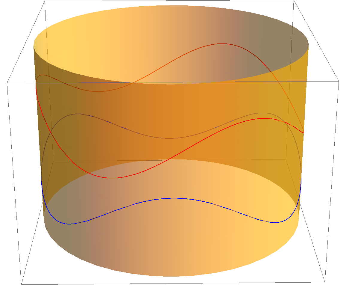
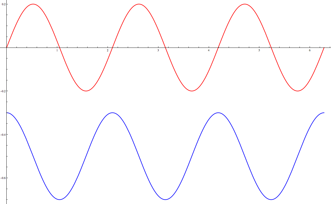
Figure 9. An admissible curve at $\partial_{\infty}\mathbb{H}^{2}\times\mathbb{R}.$

Taking the previous definition into account, we obtain the following compactness results:

Theorem 9.4 (Compactness).

Let $A_{n}$ be a sequence in A such that $\Pi(A_{n})$ converges to $\Gamma_{0}\in\Omega.$ Then, up to a subsequence, $A_{n}$ converges to a minimal annulus $A_{0}\in\mbox{\gothfamily A}^{\pi}.$

Proof.

Since $\Gamma_{0}\in\Omega$, Theorem 8.5 and Theorem 8.10 imply that $A_{n}$ is in Case I in Section 8.1, so Theorem 8.3 concludes the proof. ∎

This has an immediate consequence.

Corollary 9.5.

The map $\Pi|_{\mathcal{W}}:\mathcal{W}\rightarrow\Omega$ is proper.

If $\Gamma$ is admissible, then

$$\alpha_{\Gamma}(\theta)=\frac{d}{d\theta}\left(\gamma^{+}(\theta),\gamma^{-}(\theta)\right):\mathbb{S}^{1}\to\mathbb{C}\setminus\{0\}$$

is a smooth loop. and hence homotopic in $\mathbb{C}\setminus\{0\}$ to a standard $n$-cycle, $\alpha_{n}(\theta)={\rm e}^{{\rm i}n\theta}$. We say that $\Gamma$ is n-admissible. Given $n$-admissible curves $\Gamma_{0}$ and $\Gamma_{1}$, there exists a smooth isotopy $\Gamma_{t}$ between these amongst $n$-admissible curves.

Remark 9.6.

$\Omega$ has a countable number of path-connected components

$$\Omega_{n}:=\{\Gamma\in\Omega\;:\;\Gamma\mbox{ is n-admissible}\}.$$

Defining $\mathcal{W}_{n}:=\Pi^{-1}(\Omega_{n})\subset\mathcal{W},$ then the family of catenoids $\{C_{h}\;:\;h\in(0,\pi/2)\}$, is in the boundary of $\mathcal{W}_{n}$ for every $n\in\mathbb{Z}.$

9.3. Existence results.

Consider, for any $m\in\mathbb{N}$, $m\geq 2$, the rotation $R_{m}$, and the finite group ${\mathcal{R}}_{m}$ it generates.

Fixing $h<\pi/2$, then $\Gamma_{h}=\mathbb{S}^{1}\times\{-h,h\}\in\mathfrak{C}^{\pi}$ spans a unique centered catenoid $C_{h}$.

Proposition 9.7.

There exists an open neighborhood of $\Gamma_{h}$, $U\subset\mathfrak{C}_{m}$, such that for any $\Gamma\in U$, then there is a unique annulus $A\in\mbox{\gothfamily A}_{m}$ with $\Pi(A)=\partial A=\Gamma$.

Proof.

First notice that all the arguments in Section 6 remain true restricted to the space of ${\mathcal{R}}_{m}$-invariant functions over $C_{h}$.

By Proposition 2.2, the space of decaying Jacobi fields $\mathfrak{J}_{h}^{0}$ is generated by

$$\varphi=\frac{1-r^{2}}{r}\cos\theta,\quad\psi=\frac{1-r^{2}}{r}\sin\theta,$$

so ${\rm Ker}\left(D\left.\left(\Pi|_{\mbox{\gothfamily A}_{m}}\right)\right|_{C_{h}}\right)=\{0\}$. The Inverse Function Theorem gives neighborhoods $C_{h}\in W\subset\mbox{\gothfamily A}_{m}$ and $\Gamma_{h}\in U\subset\mathfrak{C}_{m}$ such that $\Pi|_{W}:W\rightarrow U$ is a diffeomorphism.

To prove the uniqueness, we proceed by contradiction. Assume there exists a sequence $\Gamma_{n}\in\mathfrak{C}_{m}$ with $\Gamma_{n}\to\Gamma_{h}$ and such that there are two distinct $\mathcal{R}_{m}$-invariant minimal annuli $A_{n}^{1}\neq A_{n}^{2}$, each satisfying $\Pi(A_{n}^{i})=\Gamma_{n}$. By Theorem 8.15, $A_{n}^{1}\to C_{h}$ and $A_{n}^{2}\to C_{h}$.

Write $A_{n}^{i}$ as a normal graph over $C_{h}$ of a function $u_{n}^{i}$, $i=1,2$. Define

$$v_{n}:=\left(\frac{u_{n}^{2}-u_{n}^{1}}{\|u_{n}^{2}-u_{n}^{1}\|_{\infty}}\right).$$

This vanishes on $\partial C_{h}$ since $(u_{n}^{2}-u_{n}^{1})|_{\Gamma_{h}}=0$.

Choose $p_{n}\in C_{h}$ so that $v_{n}(p_{n})=1$. If $p_{n}$ diverges in $\mathbb{H}^{2}\times\mathbb{R}$, then take a horizontal translation $T_{n}$ such that $T_{n}(p_{n})=(0,t_{n})$. Clearly $\{t_{n}\}\to\{\pm h\}$, so we choose a subsequence for which $p_{n}$ converges to a point in $\mathbb{S}^{1}\times\{h\}.$ Then $v_{n}\circ{T_{n}}^{-1}$ converges to a Jacobi field on $\mathbb{H}^{2}\times\{h\}$ which reaches a maximum at $(0,h)$. This is impossible. This proves that, up to a subsequence, $p_{n}\to p_{0}\in C_{h}$.

It is now standard to deduce the existence of a limit $v:=\lim_{n\to\infty}v_{n}$, which is a nontrivial $\mathcal{R}_{m}$-invariant element of $\mathfrak{J}^{0}(C_{h})$. However, there are no such elements. This is a contradiction, and hence we have proved the uniqueness. ∎

Remark 9.8.

Reasoning as above, we can also prove that if $A$ is ${\mathcal{R}}_{m}$-invariant and sufficiently close to $C_{h}$, then there are no ${\mathcal{R}}_{m}$-invariant elements of $\mathfrak{J}^{0}(A)$.

When $m=2$, even more is true. In the following, $U$ denotes the neighborhood of $\Gamma_{h}$ provided by Proposition 9.7 for $m=2.$

Proposition 9.9.

For every neighborhood $U^{\prime}\subset U\subset\mathfrak{C}_{2}$ containing $\Gamma_{h}$, and for any even integer $n\neq 0$, there exists $\Gamma\in U^{\prime}\cap\Omega_{n}$ such that the unique annulus $A\in\mbox{\gothfamily A}_{2}\cap\mathcal{W}_{n}$ with $\Pi(A)=\Gamma$ is non-degenerate, in the sense that $\mathfrak{J}^{0}(A)=\{0\}$.

Proof.

Since $n$ is even, we can construct a family $\{A_{\varepsilon}\}$ of minimal annuli satisfying, for all $|\varepsilon|<\varepsilon_{0}$:

1. $A_{0}=C_{h}$ and $\Pi(A_{\varepsilon})\subset U^{\prime}$;

2. $A_{\varepsilon}\in\mathcal{W}_{n}$;

3. $A_{\varepsilon}$ is $\mathcal{R}_{2}$-invariant, but not $\mathcal{R}_{2k}$-invariant, $k>1.$

By Proposition 10.1 below (see also Remark 10.2), we deduce that $A_{\varepsilon}$ is non-degenerate, for almost all $\varepsilon>0.$ ∎

Theorem 9.10.

If $n$ is even and nonzero, the projection

$$\Pi:{\mathcal{W}}_{n}\longrightarrow\Omega_{n}$$

is a proper map of degree $\pm 1\;($mod $2)$. In particular, given $\Gamma\in\Omega_{n}$, there exists a properly embedded minimal annulus such that $\Pi(A)=\Gamma.$

Proof.

By Corollary 9.5, $\Pi|_{\mathcal{W}_{n}}$ is proper. Thus $\Pi|_{\mathcal{W}_{n}}$ has a well-defined degree:

$$\deg(\Pi|_{\mathcal{W}_{n}}):=\sum_{A\in\Pi^{-1}(\Gamma)}(-1)^{{\rm index}(A)},$$

where $\Gamma$ is any regular value of $\Pi$. Regular values are generic in $\mathfrak{C}$.

The rotation $R_{2}$ is a diffeomorphism of $\mathcal{W}_{n}$. Fix $\Gamma_{0}$ in the open neighborhood ${\mathcal{U}}$ of Proposition 9.7, for $m=2$. Then $\Gamma_{0}$ spans a unique $R_{2}$-invariant annulus $A_{0}$. By Proposition 9.9 we may choose $\Gamma_{0}$ so that $A_{0}$ is non-degenerate.

Enumerate the other (non-congruent) annuli in $\Pi^{-1}(\Gamma_{0})$ by $A_{1},\ldots,A_{k}.$ If $\Gamma_{0}$ is sufficiently close to $\mathbb{S}^{1}\times\{-h,h\}$, then any non-symmetric solution $A_{i}$, $i\in\{1,\ldots,k\}$, creates $2$ different annuli $A_{i}^{j}:=R_{2}^{j}(A_{i})$, $j=0,1,$ each in $\Pi^{-1}(\Gamma_{0})$.

Let $\mathfrak{U}_{0}$ be an $R-2$-invariant neighborhood of $A_{0}$ in $\mathcal{W}_{n}$ for which $\mathfrak{J}^{0}(A)=\{0\},$ for all $A\in\mathfrak{U}_{0}$. Choose further neighborhoods $\mathfrak{U}_{i}$ of $A_{i}$ in $\mathcal{W}_{n}$, $i=1,\ldots,k$ which are pairwise disjoint from each other and fro m$\mathfrak{U}_{0}$, and such that $R_{2}(\mathfrak{U}_{i})\cap\mathfrak{U}_{j}=\varnothing,$ for all $i,j=1,\ldots,k$. Now choose $\Gamma\in\Omega_{n}$ near $\Gamma_{0}$, which is a regular value of $\Pi$ (possibly $\Gamma_{0}=\Gamma$.) Our compactness results imply that

$$\Pi^{-1}(\Gamma)\subset\bigcup_{i=0}^{k}\left(\mathfrak{U}_{i}\cup R_{2}(\mathfrak{U}_{i})\right).$$

Furthermore, clearly $\deg\left(\Pi|_{\mathfrak{U}_{i}}\right)=\deg\left(\Pi|_{R_{2}(\mathfrak{U}_{i})}\right),$ $i=1,\ldots,k$. Therefore

$$\deg(\Pi)=(-1)^{{\rm index}(A)}+2\cdot\left(\sum_{i=1}^{k}\deg\left(\Pi|_{\mathfrak{U}_{i}}\right)\right),$$

where $A$ is the unique element in $\Pi^{-1}(\Gamma)\cap\mathfrak{U}_{0}.$ This concludes the proof. ∎

9.4. The asymptotic Dirichlet problem for non-disjoint curves.

In the preceding we have considered pairs of curves $(\gamma^{+},\gamma^{-})$ satisfying $\gamma^{+}(\theta)>\gamma^{-}(\theta)$ for all $\theta$. However, we can extend these results about $R_{m}$-invariant solutions to allow boundary curves $\Gamma=(\gamma^{+},\gamma^{-})$ for which $\gamma^{+}(\theta)\geq\gamma^{-}(\theta)$ for all $\theta$, but $\gamma^{+}\not\equiv\gamma^{-}$. With this sense of $\gamma_{+}\geq\gamma_{-}$, define

$$\mathfrak{C}^{\ast}:=\{(\gamma^{+},\gamma^{-})\;:\>\;\gamma^{+}\geq\gamma^{-}\;\mbox{and}\;\sup_{\theta\in\mathbb{S}^{1}}\left(\gamma^{+}(\theta)-\gamma^{-}(\theta)\right)<\pi\}$$

$$\mathfrak{C}^{\ast}_{m}:=\{(\gamma^{+},\gamma^{-})\in\mathfrak{C}^{\ast}\;:\;\mbox{$(\gamma^{+},\gamma^{-})$ are $R_{m}$-invariant}\}$$

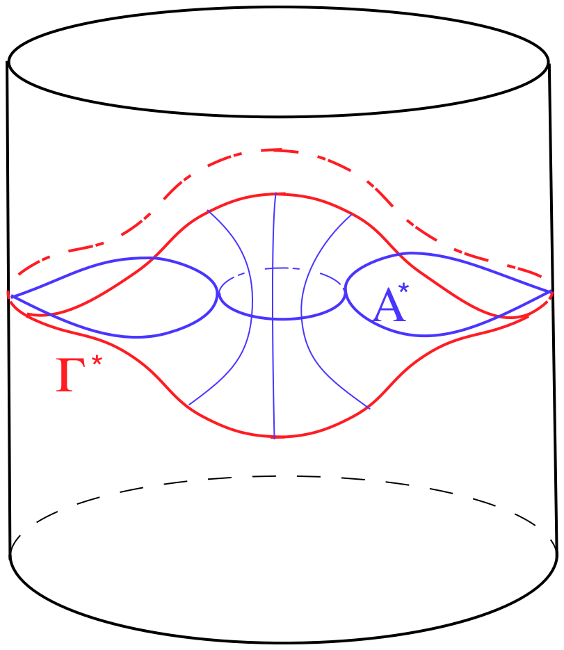
Figure 10. Annuli of this kind can be obtained as limits of our examples.

Theorem 9.11.

If $\Gamma^{*}\in\mathfrak{C}^{*}_{m}$, then there exists a complete, properly embedded minimal annulus $A^{*}$ such that $\Pi(A^{*})=\Gamma^{*}.$

Proof.

Consider a sequence of curves $\Gamma_{n}\in\mathfrak{C}_{m}$ converging to $\Gamma^{*}.$ By Theorem 9.2, for each $n$ there exists a properly embedded minimal annulus $A_{n}\in\mbox{\gothfamily A}_{m}$ such that $\Pi(A_{n})=\Gamma_{n}$. Now use Theorem 8.15 and Remark 8.17 to deduce that a subsequece of $A_{n}$ converges, smoothly on compact sets, to a minimal properly embedded minimal annulus $A^{*}$. By construction, this annulus satisfies $\Pi(A^{*})=\Gamma^{*}.$ ∎

10. Existence of nondegenerate minimal annuli

The main result of the previous section is of a somewhat general nature and does not preclude, for example, the possibility that every $A\in\mbox{\gothfamily A}$ is degenerate, i.e., that it is possible that $\mathfrak{J}^{0}(A)\neq 0$ for all $A\in\mbox{\gothfamily A}$. We prove here that this is not the case.

Proposition 10.1.

There exist minimal annuli arbitrarily near to any catenoid $A_{0}$ which are nondegenerate.

Proof.

We have proved that A is a smooth Banach manifold, so it makes sense to talk about smooth curves $A_{\epsilon}$ of minimal annuli which are deformations of the catenoid $A_{0}$. These are normal graphs over $A_{0}$ of a smooth family of functions $u_{\epsilon}$, and we set $\psi\in\mathfrak{J}(A_{0})$ to be the $\epsilon$-derivative of $u_{\epsilon}$ at $\epsilon=0$. Thus $\psi\in\mathfrak{J}(A_{0})$, so by the results in the previous section, its leading coefficients are orthogonal to the normal derivatives of every $\phi\in\mathfrak{J}^{0}(A_{0})$. In other words,

(10.1) $$(\psi_{0}^{+},\psi_{0}^{-})\perp(\cos\theta,\cos\theta),\quad(\psi_{0}^{+},\psi_{0}^{-})\perp(\sin\theta,\sin\theta).$$

Moreover, we can construct such families of minimal annuli for any Jacobi field which satisfies (10.1).

Now, within the space of Jacobi fields $\mathfrak{J}(A_{\epsilon})$, there are two distinguished subspaces: the decaying Jacobi fields $\mathfrak{J}^{0}(A_{\epsilon})$ and another space ${\mathcal{D}}(A_{\epsilon})$ consisting of Jacobi fields on $A_{\epsilon}$ generated by horizontal dilations in $\mathbb{H}^{2}\times\mathbb{R}$. We are assuming that $\mathfrak{J}^{0}(A_{\epsilon})$ is nontrivial, and standard eigenvalue perturbation theory implies that $\dim\mathfrak{J}^{0}(A_{\epsilon})\leq 2$. Furthermore, we also have that ${\mathcal{D}}(A_{\epsilon})$ converges to $\mathfrak{J}^{0}(A_{0})$ since the latter is also generated by dilations. Thus when $\epsilon\neq 0$, the two spaces are quite close to one another. We are interested in the way in which one approaches the other.

Let us first assume that $\dim\mathfrak{J}^{0}(A_{\epsilon})=2$ for all small $\epsilon$. We handle the other case later. Choose a codimension two subspace $W_{\epsilon}\subset\mathfrak{J}(A_{\epsilon})$ which varies smoothly in $\epsilon$ and which is always complementary to $\mathfrak{J}^{0}(A_{\epsilon})$ (for example, we can take an orthogonal complement with respect to some weighted Hilbert structure). Choose any smooth family $\phi_{\epsilon}\in{\mathcal{D}}(A_{\epsilon})$, and decompose it into components in each of these subspaces, $\phi_{\epsilon}=\psi_{\epsilon}+w_{\epsilon}$, where $\psi_{\epsilon}\in\mathfrak{J}^{0}(A_{\epsilon})$ and $w_{\epsilon}\in W_{\epsilon}$. Note that $w_{\epsilon}$ and $\phi_{\epsilon}$ agree at $\partial A_{\epsilon}$.

We now observe that the map which assigns to any $w\in W_{\epsilon}$ its leading coefficients, i.e., boundary values, $(w_{0}^{+},w_{0}^{-})$, has image equal to a codimension $2$ subspace of $({\mathcal{C}}^{2,\alpha}(\mathbb{S}^{1}))^{2}$ which depends smoothly on $\epsilon$ and which equals the subspace given by the orthogonality conditions (10.1) when $\epsilon=0$. This map is, by definition, injective and also surjective. Hence by the open mapping theorem, the norm of any $w\in W_{\epsilon}$ is equivalent to the norm of its boundary values. This means that the rescaled sequence of functions

$$\tilde{w}_{\epsilon}=w_{\epsilon}/\sup_{\partial A_{\epsilon}}|w_{\epsilon}|$$

is uniformly bounded, independently of $\epsilon$, and always attains the value $1$ at some point of the boundary. Thus it has a well defined limit, $\tilde{w}$, which is therefore an element of $\mathfrak{J}(A_{0})$. Its boundary values must satisfy (10.1).

Now let us compute the boundary values of the original Jacobi field $\phi_{\epsilon}$. Parametrizing the boundary curves of $A_{\epsilon}$ by the functions $f_{\epsilon}^{\pm}(\theta)$, suppose that $D_{\lambda}$ is a family of horizontal dilations and let $A_{\epsilon,\lambda}=D_{\lambda}(A_{\epsilon})$, corresponding in turn to a family of normal graphs over $A_{\epsilon}$ by a family of functions $u_{\epsilon,\lambda}$. We calculate readily that at $r=1$ and at the upper and lower halves, up to an overall constant factor,

$$\left.\frac{d\,}{d\lambda}u_{\epsilon,\lambda}(1,\theta)\right|_{\lambda=0}=(\sin(\theta+\beta)(f_{\epsilon}^{+})^{\prime}(\theta),\sin(\theta+\beta)(f_{\epsilon}^{-})^{\prime}(\theta)),$$

for some $\beta$ depending on the family of dilations. This is equal to the pair boundary values of the Jacobi field $w_{\epsilon}$, and hence also of the Jacobi field $\tilde{w}_{\epsilon}$.

In the final limit, we are dividing by the supremum of $\sin(\theta+B)(f_{\epsilon}^{\pm})^{\prime}$ and letting $\epsilon\to 0$. However, this is equivalent to taking the derivative in $\epsilon$ of this family. By the earlier definition, the derivative of $f_{\epsilon}^{\pm}$ with respect to $\epsilon$ equals the Jacobi field $\psi$ on $A_{0}$. This proves finally that the boundary values of the limiting Jacobi field $\tilde{w}$ above must be

(10.2) $$(\tilde{w}_{0}^{+},\tilde{w}_{0}^{-})=(\sin(\theta+\beta)(\psi_{0}^{+})^{\prime}(\theta),\sin(\theta+\beta)(\psi_{0}^{-})^{\prime}(\theta)).$$

Now let us choose the Jacobi field $\psi$ generating the family $A_{\epsilon}$. Expanding boundary values into their Fourier series

$$\psi_{0}^{\pm}(\theta)=\sum_{k=0}^{\infty}(a_{k}^{\pm}\cos k\theta+b_{k}^{\pm}\sin k\theta)$$

then the constraint (10.1) is equivalent to two conditions $a_{1}^{+}+a_{1}^{-}=b_{1}^{+}+b_{1}^{-}=0$, and apart from these, all the other Fourier coefficients can be chosen arbitrarily (sufficiently small, of course, and so that the resulting function has the correct regularity). However, evaluating the expressions on the right in (10.2) yields a function which contains

$$\underbrace{(-a_{2}^{\pm}\cos\beta+b_{2}^{\pm}\sin\beta)}_{B_{1}^{\pm}}\cos\theta+\underbrace{(-b_{2}^{\pm}\cos\beta-a_{2}^{\pm}\sin\beta)}_{B_{2}^{\pm}}\sin\theta$$

for any choice of $B_{1}^{\pm}$, $B_{2}^{\pm}$, since these coefficients depend only on the coefficients $a_{2}^{\pm},b_{2}^{\pm}$. However, this is a contradiction, since these are the leading coefficients of the element of $\tilde{w}\in\mathfrak{J}$. This proves that it is impossible that $\dim\mathfrak{J}^{0}(A_{\epsilon})=2$ for all $\epsilon$.

We are reduced to the case where $\dim\mathfrak{J}^{0}(A_{\epsilon})=1$ for almost every $\epsilon$. In the preceding part of the proof, it is not hard to argue slightly differently to show that in fact there cannot even exist a sequence $\epsilon_{j}\searrow 0$ for which $\dim\mathfrak{J}^{0}(A_{\epsilon})=2$ and with appropriate Fourier coefficients nonzero, so we can assume that the dimension is $1$ for all $\epsilon\neq 0$. In this case we can actually still proceed almost as before. The difference is that the family of dilations $D_{\lambda}$ generating $A_{\epsilon,\lambda}$ is no longer arbitrary. Instead, observe that the eigenspace $\mathfrak{J}^{0}(A_{\epsilon})$ (at least along a sequence $\epsilon_{j}\searrow 0$) must have a limit $E_{0}$, which is a one-dimensional subspace of $\mathfrak{J}^{0}(A_{0})$ Since ${\mathcal{D}}(A_{\epsilon})\to\mathfrak{J}^{0}(A_{0})$ smoothly, we can choose a subspace $E_{\epsilon}\subset{\mathcal{D}}(A_{\epsilon})$ which converges smoothly to $E_{0}$. It is now clear that the difference vector $w_{\epsilon}$ defined in the earlier step of the proof may still be chosen so that its normalization has a limit as $\epsilon\to 0$. The remainder of the argument proceeds exactly as before. ∎

Remark 10.2.

It is not hard to see from this argument that we can produce families of solutions $A_{\epsilon}$ converging to $A_{0}$ which are nondegenerate and also invariant with respect to rotation by $\pi$ around the axis of $A_{0}$. These are important in one of our global existence theorems (Proposition 9.9 and Theorem 9.10).

Appendix A Two tall rectangles are not area-minimizing

The purpose of this appendix is to prove that a couple of tall rectangles in $\mathbb{H}^{2}\times\mathbb{R}$ of the same height with the vertical segments in common are not an area-minimizing surface. Recall that for a complete surface area-minimizing means that any compact piece minimizes the area among all the surfaces with the same boundary. To prove this, we are going to see that, in general, a couple of horizontal disks connected by vertical totally geodesic planes near infinity (see Figure 11) are better competitors for the area functional.

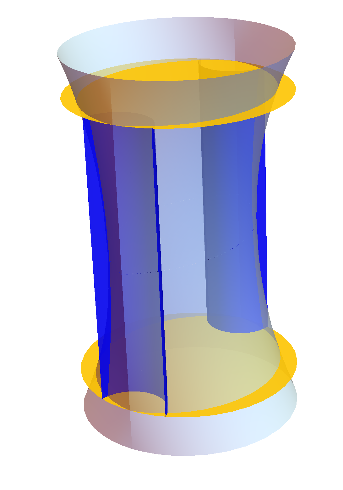
Figure 11. The tall rectangles, the horizontal disks and the vertical totally geodesic planes.

The simplest analytic representation of these surfaces is obtained using the upper half-space model for $\mathbb{H}^{2}$. Thus we use standard coordinates $(x,y)\in\mathbb{H}^{2}$ with $y>0$, and hence coordinates $(x,y,t)$ on $\mathbb{H}^{2}\times\mathbb{R}$. We shall place the vertical segments of the tall rectangles over the points $(0,0)$ and infinity. For a given $r>0$ we denote $\Gamma_{r}$ the geodesic in $\mathbb{H}^{2}$ with end points $(r,0)$ and $(-r,0)$. Let $P_{r}:=\Gamma_{r}\times\mathbb{R}$ be the corresponding totally geodesic plane. For simplicity we will write $\Gamma=\Gamma_{1}$ and $P=P_{1}$. Finally, we denote $\Lambda$ as the geodesic given by $\{x=0,y>0\}$. The point in the intersection $\Gamma\cap\Lambda$ is denoted by $o=(0,1)$.

On the geodesic $\Gamma$ we consider $\rho$ the signed distance to the point $o$. Then the induced metric in $P$ is given by $d\rho^{2}+dt^{2}.$ We write a curve in $P$ in coordinates $(\rho,t)$ of the form

$$\rho\mapsto(\rho,\lambda(\rho)).$$

If we impose that the surface generated by horizontal translations along the geodesic $\Lambda$ of the above curve is minimal, then we get (see [18, page 316]) that the function $\lambda(\rho)$ satisfies the equation

(A.1) $$\lambda^{\prime}(\rho)=\frac{d}{\sqrt{\cosh^{2}\rho-d^{2}}},\quad d\geq 0.$$

If $d>1$ we have

(A.2) $$\lambda(\rho)=\int_{\cosh^{-1}(d)}^{\rho}\frac{d}{\sqrt{\cosh^{2}u-d^{2}}}du.$$

We parametrize $\Gamma$ as $\theta\mapsto{\rm e}^{{\rm i}\theta},$ $\theta\in(0,\pi).$ Then it is straightforward to check that

$$\rho=\log\left(\tan\frac{\theta}{2}\right).$$

Combining the above expression and (A.1) then we obtain:

(A.3) $$\lambda^{\prime}(\theta)=\frac{d\csc(\theta)}{\sqrt{\csc^{2}(\theta)-d^{2}}},$$

and

$$\lambda(\theta)=\int_{\theta}^{\theta_{0}}\frac{d\csc(t)}{\sqrt{\csc^{2}(t)-d^{2}}}dt,\quad\theta_{0}=\csc^{-1}(d).$$

So the upper half part of the tall rectangle is given by the parametrization

(A.4) $$\phi(r,\theta)=(r\cos(\theta),r\sin(\theta),\lambda(\theta)),\;\;r\in(0,\infty),\;\;\theta\in(0,\theta_{0}).$$

The lower half part is parametrized by $(r,\theta)\mapsto(r\cos(\theta),r\sin(\theta),-\lambda(\theta)).$ Let $R_{1}$ be the complete tall rectangle described above.

The height of the tall rectangle $R_{1}$ is given by $2\lambda(0)>\pi$. Moreover, notice that the intersection of the tall rectangle with the slice $t=\lambda(\theta)$ consists of the straight line $\{r{\rm e}^{{\rm i}\theta}\;:\;r>0\}.$

Let $R_{2}$ be the tall rectangle obtained from $R_{1}$ applying the symmetry $(x,y,t)\mapsto(-x,y,t).$

Fix $r\in(0,1)$ and $\theta\in(0,\theta_{0})$. We consider the two horizontal slices, $S_{\lambda(\theta)}$ and $S_{-\lambda(\theta)}$, at height $\lambda(\theta)$ and $-\lambda(\theta)$, respectively, and the two vertical planes $P_{r}$ and $P_{1/r}.$ We cut the tall rectangles $R_{1}\cup R_{2}$ with the union

$$S_{\lambda(\theta)}\cup S_{-\lambda(\theta)}\cup P_{r}\cup P_{1/r}.$$

The resulting curve is a compact curve in $R_{1}\cup R_{2}$ with two connected components: $\beta_{i}\subset R_{i}$, $i=1,2.$ These two curves are symmetric with respect to the plane $x=0$. Let $\Sigma_{i}$ the disk in $R_{i}$ spanned by $\beta_{i}$, $i=1,2$. Observe that $\Sigma_{i}$ is a symmetric bi-graph over the annular sector $\Delta_{i}$ (see Figure 12.) Moreover we will denote:

• $D_{1}=\{(u\cdot{\rm e}^{{\rm i}v},\lambda(\theta))\;:\;(u,v)\in(r,1/r)\times(\theta,\pi-\theta)\}.$

• $D_{2}=\{(u\cdot{\rm e}^{{\rm i}v},-\lambda(\theta))\;:\;(u,v)\in(r,1/r)\times(\theta,\pi-\theta)\}.$

• $B_{1}$ the region of $P_{r}$ bounded by $\beta_{1}\cup\beta_{2}$ and the curves $D_{1}\cap P_{r}$ and $D_{2}\cap P_{r}$.

• $B_{2}$ the region of $P_{1/r}$ bounded by $\beta_{1}\cup\beta_{2}$ and the curves $D_{1}\cap P_{1/r}$ and $D_{2}\cap P_{1/r}$.

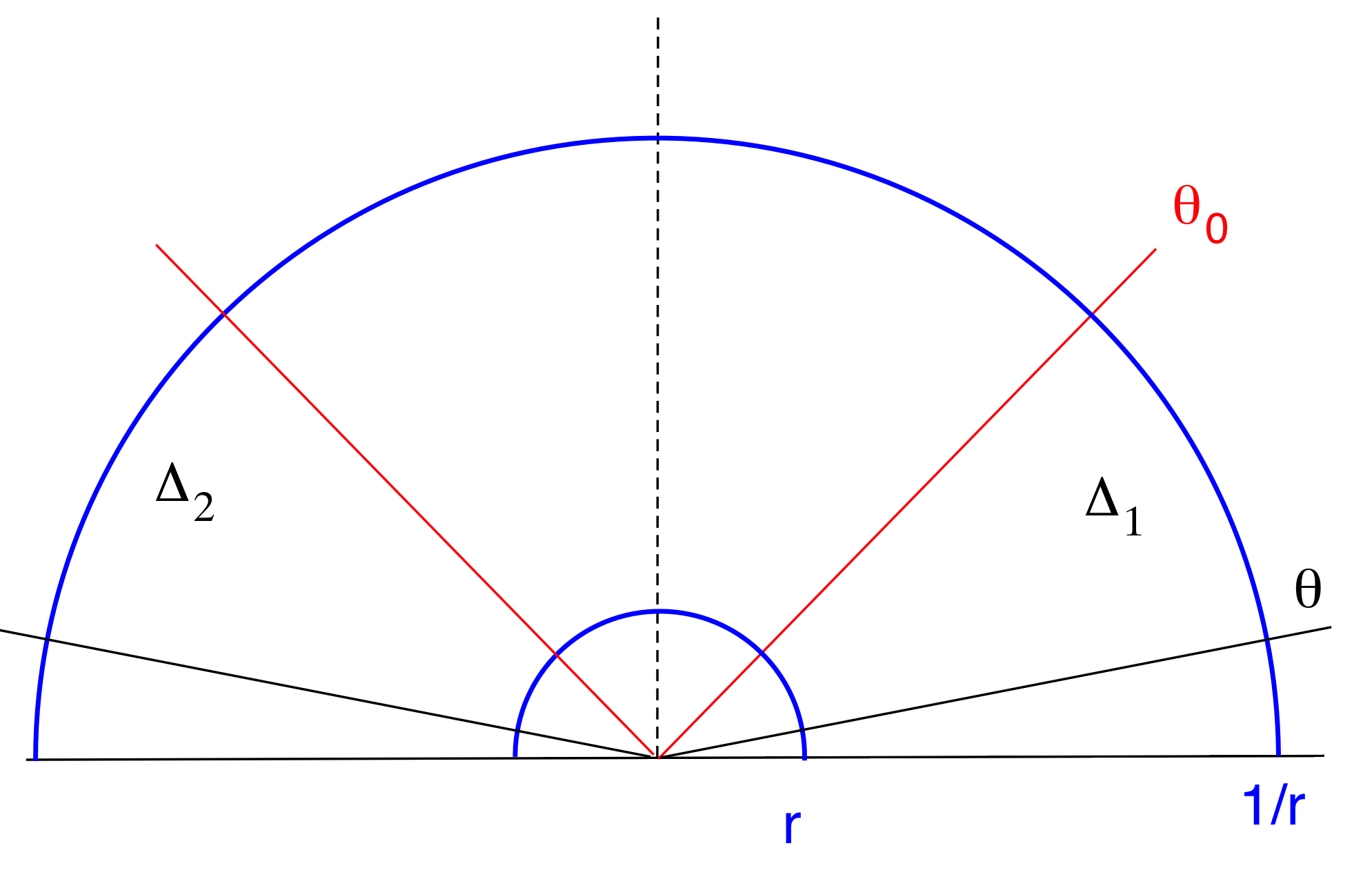
Figure 12. The annular sectors $\Delta_{1}$ and $\Delta_{2}.$

We want to prove that

Lemma A.1.

The area of the region $D_{1}\cup D_{2}\cup B_{1}\cup B_{2}$ is smaller than the area of $\Sigma_{1}\cup\Sigma_{2}$. In particular, $R_{1}\cup R_{2}$ is not area-minimizing.

Proof.

By the symmety of the surface it is enough to prove that for some $\theta$ and $r$

$$\frac{Area(\Sigma_{1})}{Area(D_{1})+Area(B_{1})}>1\;.$$

From (A.4) it is not difficult to see that

$$A_{1}(r,\theta) := Area(\Sigma_{1})=-2\log(r)\left(\cot(\theta)\sqrt{4-2d^{2}+2d^{2}\cos(2\theta)}+2E(\theta|d^{2})-2F(\theta|d^{2})\right.$$

$$- \left.\cot(\theta_{0})\sqrt{4-2d^{2}+2d^{2}\cos(2\theta_{0})}-2E(\theta_{0}|d^{2})+2F(\theta_{0}|d^{2})\right)\;,$$

where $E$ and $F$ are the classical elliptic functions given by

$$E(\Phi|m)=\int_{0}^{\Phi}\sqrt{1-m\sin^{2}(s)}ds\quad,\quad F(\Phi|m)=\int_{0}^{\Phi}\frac{1}{\sqrt{1-m\sin^{2}(s)}}ds\;.$$

Similarly, we have

$$A_{2}(r,\theta):=Area(D_{1})=-4\log(r)\cot(\theta)\;.$$

Finally, observe that $Area(B_{1})$ is less than the area of the region in $P_{r}$ given by

$$\{(r\cdot{\rm e}^{{\rm i}v},t)\;:\;v\in(\theta,\pi-\theta),t\in(-\lambda(0),\lambda(0))\}.$$

So,

$$Area(B_{1})<A_{3}(\theta):=2\lambda(0)\log\left(\cot^{2}\left(\frac{\theta}{2}\right)\right)\;.$$

Now we take $r(\theta)=\tan^{n}\left(\frac{\theta}{2}\right)$, where $n\in\mathbb{N}$ will be taken big enough in terms of $d$. Notice that for this choice of $r$ we have

$$\frac{Area(\Sigma_{1})}{Area(D_{1})+Area(B_{1})}>f(\theta):=\frac{A_{1}(r(\theta),\theta)}{A_{2}(r(\theta),\theta)+A_{3}(\theta)}\;.$$

It is straitforward that

$$\lim_{\theta\to 0}f(\theta)=1\quad,\quad\lim_{\theta\to 0}f^{\prime}(\theta)=-\frac{\lambda(0)}{n}+F\left(\theta_{0}\left|\csc^{2}(\theta_{0})\right.\right)-E\left(\theta_{0}\left|\csc^{2}(\theta_{0})\right.\right).$$

As $F\left(\theta_{0}\left|\csc^{2}(\theta_{0})\right.\right)-E\left(\theta_{0}\left|\csc^{2}(\theta_{0})\right.\right)>0$, then

$$\lim_{\theta\to 0}f^{\prime}(\theta)>0$$

for $n$ big enough. So, we have that for $\theta$ small enough $f(\theta)>1$, which proves our lemma. ∎

References

- [1] P. Collin, L. Hauswirth and H. Rosenberg. Properly immersed minimal surface in a slab of , the hyperbolic plane. Arch. Math. 104 (2015), 471–484.
- [2] B. Coskunuzer. Minimal Surfaces with Arbitrary Topology in . Preprint arXiv:1404.0214.
- [3] B. Coskunuzer. Asymptotic Plateau Problem in . Selecta Math. (to appear.)
- [4] B. Daniel. Isometric immersions into and and applications to minimal surfaces. Trans. A.M.S. 361 (2009), 6255–6282.
- [5] L. Hauswirth. Minimal surfaces of Riemann type in three-dimensional product manifolds, Pacific J. Math., 224 (2006), 91–117.
- [6] L. Hauswirth, A. Menezes and M. Rodríguez. On the characterization of minimal surfaces with finite total curvature in and . Preprint arXiv:1604.07083.
- [7] B. Kloeckner and R. Mazzeo. On the asymptotic behavior of minimal surfaces in . Indiana Math J. 66 no. 2 (2017), 631–658.
- [8] F. Martín, R. Mazzeo and M. Rodríguez. Minimal surfaces with positive genus and finite total curvature in . Geometry and Topology 18 (2014) 141–177.
- [9] L. Mazet, M. Rodríguez and H. Rosenberg. The Dirichlet problem for the minimal surface equation -with possible infinite boundary data- over domains in a Riemannian surface. Proc. London Math. Soc., 102 (2011), no. 3, 985–023.
- [10] L. Mazet, M. Rodríguez and H. Rosenberg. Periodic constant mean curvature surfaces in . Asian J. Math., 18 (2014), no. 5, 829–858.
- [11] R. Mazzeo. Elliptic theory of differential edge operators, I. Comun. Par. Diff. Eq. 16(1991), 1616–1664.
- [12] R. Mazzeo and F. Pacard. Constant mean curvature surfaces with Delaunay ends. Comm. Anal. Geom. 9 (2001) no. 1, 169–237.
- [13] F. Morabito. A Costa-Hoffman-Meeks type surface in . Trans. Amer. Math. Soc., 363 (2011), no. 1, 1–36.
- [14] B. Nelli and H. Rosenberg. Minimal surfaces in . Bull. Braz. Math. Soc. (N.S.) 33 (2002), no. 2, 263–292. Errata: Bull. Braz. Math. Soc. (N.S.) 38 (2007), no. 4, 661–664.
- [15] B. Nelli, R. Sa Earp and E. Toubiana. Maximum principle and symmetry for minimal hypersurfaces in . Ann. Sc. Norm. Super. Pisa Cl. Sci. (5) Vol. XIV (2015), 387–400.
- [16] R. Sa Earp. Parabolic and hyperbolic screw motion surfaces in . J. Australian Math. Soc. 85 (2008), 113–143.
- [17] R. Sa Earp and E. Toubiana. Screw motion surfaces in and . Illinois J. Math. 49 (2005), no. 4, 1323–1362.
- [18] R. Sa Earp and E. Toubiana. An asymptotic theorem for minimal surfaces and existence results for minimal graphs in , Mathematische Annalen, 342 (2) (2008), 309–331.
- [19] X. Mo and R. Osserman. On the Gauss map and total curvature of complete minimal surfaces and an extension of Fujimoto’s theorem. J. Differential Geom. 31, no. 2 (1990), 343–355.
- [20] B. White. The space of -dimensional surfaces that are stationary for a parametric elliptic functional. Indiana Univ. Math. J. 36, no. 3 (1987), 567–602.
- [21] B. White. The maximum principle for minimal varieties of arbitrary codimension. Comm. Anal. Geom. 18 (2010), no. 3, 421–432.
- [22] B. White. Controlling area blow-up in minimal or bounded mean curvature varieties. J. Differential Geom. 102, no. 3 (2016), 501–535.
- [23] B. White. On the compactness theorem for embedded minimal surfaces in 3-manifolds with locally bounded area and genus. Comm. Anal. Geom. 26, no. 3 (2018), 659–678.