Extreme submillimetre starburst galaxies

We use two catalogues, a Herschel catalogue selected at 500 $\mu$m (HerMES) and an IRAS catalogue selected at 60 $\mu$m (RIFSCz), to contrast the sky at these two wavelengths. Both surveys demonstrate the existence of “extreme” starbursts, with star-formation rates (SFRs) $>5000M_{\odot}yr^{-1}$. The maximum intrinsic star-formation rate appears to be $\sim 30,000M_{\odot}yr^{-1}$. The sources with apparent SFR estimates higher than this are in all cases either lensed systems, blazars, or erroneous photometric redshifts.

At redshifts of 3 to 5, the time-scale for the Herschel galaxies to make their current mass of stars at their present rate of star formation $\sim 10^{8}$ yrs, so these galaxies are making a significant fraction of their stars in the current star-formation episode. Using dust mass as a proxy for gas mass, the Herschel galaxies at redshift 3 to 5 have gas masses comparable to their mass in stars. Of the 38 extreme starbursts in our Herschel survey for which we have more complete spectral energy distribution (SED) information, 50$\%$ show evidence for QSO-like optical emission, or exhibit AGN dust tori in the mid-infrared SEDs. In all cases however the infrared luminosity is dominated by a starburst component. We derive a mean covering factor for AGN dust as a function of redshift and derive black hole masses and black hole accretion rates. There is a universal ratio of black-hole mass to stellar mass in these high redshift systems of $\sim 10^{-3}$, driven by the strong period of star-formation and black-hole growth at $z=1-5$.

1 Introduction

A key discovery from the Infrared Astronomical Satellite (IRAS) surveys was the existence of galaxies with remarkably high infrared (rest-frame $1-1000\,\mu$m) luminosities. IRAS found thousands of galaxies with infrared luminosities $>10^{12}L_{\odot}$, termed “ultraluminous” infrared galaxies or ULIRGs (Soifer et al 1984, Aaronson and Olszewski 1984, Houck et al 1985, Joseph and Wright 1985, Allen et al 1985, Lawrence et al 1986), and over a hundred with luminosities $>10^{13}L_{\odot}$, termed “hyperluminous” infrared galaxies or HyLIRGs (Rowan-Robinson et al 2000, Rowan-Robinson and Wang 2010). All-sky surveys in the mid-infrared with WISE also uncovered comparably luminous systems (Eisenhardt et al 2012). While rare locally, infrared-luminous systems rise dramatically in number with increasing redshift, until at $z>1$ they host a substantial, possibly dominant fraction of the comoving infrared luminosity density (Le Floc’h et al 2005, Perez-Gonzalez et al 2005). Infrared template modelling, and other follow-up, has shown that both starbursts and AGN dust tori can contribute to these very high infrared luminosities, with implied star formation rates (SFRs) exceeding $1000\,M_{\odot}$ yr^-1. Selection at 22 (WISE) or 25 (IRAS) $\mu$m favours dominance by AGN dust tori, while selection at 60 $\mu$m or longer wavelengths favours dominance by star formation. In order to obtain the most robust selection possible we here use infrared template modelling to select sources on the basis of their star-formation rate, rather than their infrared luminosity.

More recent surveys at longer wavelengths by Herschel have drawn attention to even more extreme objects, with star-formation rates in excess of $10,000\,M_{\odot}yr^{-1}$ in some cases (Rowan-Robinson et al 2016). The existence of these “extreme” starbursts poses a fundamental problem for semi-analytic models of galaxy formation. The observed number density of extreme starbursts with SFRs$>$1000 M_⊙yr^-1 (Dowell et al 2014, Asboth et al 2016) is factors of several above model predictions, while the extreme starbursts with SFRs $>$ 3000 M_⊙yr^-1 do not exist at all in models (Lacey et al 2010, 2016, Gruppioni et al 2011, 2015, Hayward 2013, Henriques et al 2015). The issue for the models is that neither mergers or cold accretion should produce such high SFRs; mergers because they cannot channel enough gas to the centers of haloes (e.g. fig. 1 of Narayanan et al 2010, Dave et al 2010), and cold accretion because massive haloes inhibit the gas flow on to central galaxies via shock heating (Birnbolm and Dekel 2003, Keres et al 2005, Narayanan et al 2015). The models could potentially reproduce SFRs of $>$3000 M_⊙yr^-1 at $z>1$ if feedback is turned off completely, but would then strongly overpredict the $z=0$ galaxy mass function.

There is thus a pressing need to confirm the existence of systems with such high star formation rates, especially at high redshifts, understand how efficient surveys at different wavelengths are at uncovering them, and to understand the relation between their stellar mass and black hole mass assembly events. In this paper we undertake such a study, by examining and contrasting the selection of extreme starburst galaxies from two surveys, one at 60 $\mu$m and one at 500 $\mu$m. There are four reasons for using a 60 $\mu$m (IRAS) sample as well as a 500 $\mu$m one. Firstly the contrast between 500 and 60 $\mu$m surveys brings out what is distinct about the 500 $\mu$m sky. Secondly we find that the 60 $\mu$m sample helps us delineate the maximum possible rate of star-formation in galaxies (section 4). Thirdly our 60 $\mu$m survey is free of the problems of confusion and blending which are issues at submillimetre wavelengths, because of the small numbers of sources per beam. Confusion only became an issue for IRAS in the Galactic plane and in the very deepest IRAS surveys at the North Ecliptic Pole (Hacking and Houck 1987). Finally in our analysis of AGN (section 7) the 60 $\mu$m sample provides us with a useful low redshift benchmark.

This paper is structured as follows. Section 2 describes our sample selection strategy from the IRAS and Herschel surveys. In section 4 we outline how candidate lenses are removed from the samples. We then describe how stellar masses, gas masses, and star formation rates are computed for each source in section 5. Using these derived quantities, we then examine the properties of the extreme starbursts in the sample in section 6, and the role of AGN in section 7.

A cosmological model with $\Lambda=0.7$, $h_{0}=0.72$ has been used throughout. If we were to use $H_{0}=67km/s/Mpc$ (Planck collaboration 2014) then luminosities and star-formation rates would increase by 15.5$\%$.

2 Sample Selection

We select sources from two catalogs; the Revised IRAS Faint Source Survey Redshift Catalogue (RIFSCz, Wang et al 2014), and the Herschel Multi-tiered Extragalactic Survey (HerMES, Oliver et al 2012). Below, we describe each catalogue in turn.

2.1 IRAS

The Revised IRAS Faint Source Survey Redshift (RIFSCz) Catalogue (Wang et al 2014a) is a 60 $\mu$m survey for galaxies over the whole sky at $|b|>20^{o}$, which incorporates data from the SDSS, 2MASS, WISE, and Planck all-sky surveys to give wavelength coverage from 0.36-1380 $\mu$m. Since publication of Wang et al (2014) Akari fluxes have been added to the catalogue, using a search radius of 1 arc min. An aperture correction needs to be applied to Akari 65 and 90 $\mu$m fluxes to give consistency with IRAS photometry (Rowan-Robinson and Wang 2015). Furthermore the optical and near-infrared photometry of 1271 catalogued nearby galaxies has been improved, following a systematic trawl through the NASA$/$IPAC Extragalactic Database. Wang et al (2014) found that 93$\%$ of RIFSCz sources had optical or near infrared counterparts with spectroscopic or photometric redshifts. The photometric redshifts primarily make use of 2MASS and SDSS photometric data. Thus for 93$\%$ of the catalogue the prime selection effect is the 60 $\mu$m sensitivity limit of the IRAS Faint Source Survey ($\sim 0.36mJy$). Table 1 summarises the number of RIFSCz galaxies by waveband.

Table 1: RIFSCz catalogue by band

Wavelength	Survey	Number of
($\mu$m)		sources
3.4	WISE	48603
4.6	WISE	48603
12	WISE	48591
12	IRAS	4476
22	WISE	48588
25	IRAS	9608
60	IRAS	60303
65	AKARI	857
90	AKARI	18153
100	IRAS	30942
140	AKARI	3601
160	AKARI	739
350	PLANCK	2275
550	PLANCK	1152
850	PLANCK	616
1380	PLANCK	150

2.2 Herschel

The HerMES survey allows us to construct a 500 $\mu$m sample of galaxies in areas in which we have deep optical and infrared data from the Spitzer-SWIRE survey (Lonsdale et al 2003, Rowan-Robinson et al 2008, 2014, 2016) over a total area of 26.3 sq deg in five fields (see Table 1 of Rowan-Robinson et al 2016). Aperture corrections are applied at optical, near and mid-infrared wavelengths to ensure that all SEDs are based on integrated flux-densities (Rowan-Robinson et al 2013). Selection at 500 $\mu$m, rather than say 250 $\mu$m, gives us greater visibility of the high redshift (z$>$3) universe due to the intrinsic shape of starburst SEDs at far-infrared wavelengths (Franceschini et al 1991) and has the benefit of ensuring detection also at 350, and in most cases 250 $\mu$m, to give valuable SED information. The association of Herschel sources with SWIRE 24$\mu$m sources uses a likelihood which combines the positional disagreement between 250$/$350$\mu$m and 24$\mu$m positions and the agreement of the observed 500$\mu$m flux with that predicted from automatic template fits to the SWIRE 4.5-170$\mu$m data. We have argued previously (Rowan-Robinson et al (2014) that the use of SED information is essential in the association process. Assignment of submillimetre flux to counterparts based purely on positional agreement can lead to physically unrealistic SEDs. The complete HerMES-SWIRE 500 $\mu$m catalogue comprises sources in the Lockman, XMM, ELAIS-S1, ELAIS-N1 and CDF-S fields, and consists of 2181 galaxies. In the Lockman+XMM+ELAIS-S1 areas there are a further 833 good quality 500+350 $\mu$m sources which are not associated with Spitzer-SWIRE galaxies, for which Rowan-Robinson et al (2016) have estimated redshifts from their submillimetre colours. Thus for all HerMES 500$\mu$m sources we have an estimate of redshift and hence of infrared luminosity (and star-formation rate). The prime selection effect on this sample is therefore the 500 $\mu$m flux-density limit of the survey.

We performed a check of the surface density of 500 $\mu$m sources in the HerMES survey using data from the COSMOS area (Scoville et al 2007), which was surveyed as part of the HerMES project. Photometric redshifts for COSMOS have been discussed by Ilbert et al (2013) and Laigle et al (2016). There are 181 500 $\mu$m sources with flux greater than 25 mJy, the flux limit we used in Rowan-Robinson et al (2016), and which also have 350 $\mu$m detections, in the 2.0 sq deg of the COSMOS survey. All have 24 $\mu$m associations. This yields a 500 $\mu$m source-density of 90 per sq deg, similar to that found in the 26.3 sq deg of our sample.

2.3 Comparison with other studies

Schulz et al (2017) have published a new IPAC SPIRE catalogue (HPSC) which analyses data taken in all Herschel SPIRE programmes in a homogeneous way, using a blind source detection approach. This would appear to offer the opportunity of a much larger sample of SPIRE galaxies. We used the HPSC catalogue to create a 250-350-500 $\mu$m list as in Rowan-Robinson et al (2014). When we associated this list with the SWIRE photometric redshift catalogue (Rowan-Robinson et al 2013), we found only about half of the 2181 sources. This is an issue acknowledged in the HPSC explanatory supplement, which they attribute to blending of SPIRE sources in their detection procedure.

We also associated this HPSC 500 $\mu$m catalogue with RIFSCz, finding 1640 associations. Many of these were also detected by Planck and so we can make a direct comparison of 350 and 500 $\mu$m fluxes in the two surveys. The sources in common to HPSC, RIFSCz and Planck tend to be low redshift galaxies. We find that these galaxies need an aperture correction of k*delmag to the SWIRE fluxes, where delmag = $J_{ext}-J_{ps}$ is the J-band aperture correction and k=0.15 at 350, and 0.10 at 500 $\mu$m, to get agreement of SPIRE and Planck fluxes. Previously Wang et al (2014) reported the need for aperture corrections to be applied to WISE fluxes at 12 and 22 $\mu$m. The latest version of RIFSCz (http:$//$mattiavaccari.net:$/$df$/$mrr$/$readmeRIFSCz) thus provides a comprehensive collection of fluxes, with aperture corrections where necessary, from optical (SDSS), near infrared (2MASS), mid and far infrared (WISE, IRAS, Akari), through to submillimetre and millimetre (Herschel and Planck).

Koprowski et al (2017) have used a SCUBA2 survey at 850 $\mu$m to estimate the rest-frame 250 $\mu$m luminosity-density and then translated this to a star-formation-rate-density assuming a universal submillimetre SED. They cast doubt on the reality of the high star-formation rates found by Rowan-Robinson et al (2016) at z = 4-6. There are some flaws in the Koprowski et al analysis. Firstly their 850 $\mu$m detection threshold is set at 3.5 $\sigma$, which means they are heavily into the confusion regime. Our strategy of thresholding at 5 $\sigma$, made possible by the excellent submillimetre sensitivity of Herschel-SPIRE, ensures that problems of confusion and source blending are greatly reduced (see section 3). Secondly, they associate their submillimetre sources with other multi wavelength data using the nearest bright 8 or 24 $\mu$m, or 1.4 GHz, source, thus potentially biassing their associations against more probable (in terms of their SED) higher redshift galaxies. Finally because their survey is at a single submillimetre wavelength they have no reliable way of estimating the star-formation rate. It is simply not true that all submillimetre galaxies have a common submillimetre SED (e.g. Rowan-Robinson et al 2014). The high star-formation rates we find are supported by the IRAS RIFSCz sample (see section 5 below) which is not subject to any of the submillimetre confusion or blending issues. Novak et al (2017) have nicely confirmed Rowan-Robinson et al (2016)’s star-formation-rate-density from z = 0 to 5 with radio estimates from a VLA survey.

Table 2: Contrast between the 60 $\mu$m selected RIFSCz catalogue and the 500 $\mu$m selected catalogue from the HerMES survey

	IRAS-FSS	HerMES-SWIRE
	60 $\mu$m	500 $\mu$m
number of sources	60303	2181
effective area (sq deg)	27143	26.3
surface-density of lensed galaxies	0.001 per deg2	10 per deg2
fraction of Ultraluminous galaxies	8 $\%$	70$\%$
fraction of Hyperluminous galaxies	0.7$\%$	25$\%$
fraction of galaxies with standard cirrus	42$\%$	34$\%$
fraction of galaxies with cool or cold cirrus	2.5$\%$	29$\%$
redshift $>$ 0.3	4$\%$	88$\%$

Table 2 shows a comparison of the sky seen at 60 and at 500 $\mu$m, as seen in the RIFSCz and HerMES-SWIRE catalogues (Rowan-Robinson et al 2014). The most striking contrasts of 500$\mu$m selection, compared to 60 $\mu$m selection, are (i) a much higher fraction of high redshift galaxies (as predicted by Franceschini et al 1991), (ii) a much higher fraction of lensed objects (as predicted by Blain et al 2002), (iii) a much higher fraction of galaxies with cool or cold dust (RR et al 2010, 2016, Rowan-Robinson and Clements 2015).

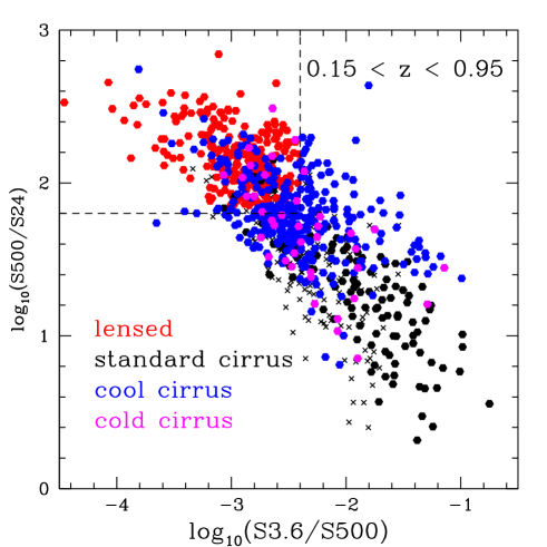
Figure 1: $S_{24}/S_{500}$ vs. $S_{3.6}/S_{500}$, illustrating the diagnostic ratios used by Rowan-Robinson et al (2014) to select lensed objects, here plotted for the sources in HerMES (Lockman+XMM+ELAIS S1+CDF-S+ELAIS N1) with $0.15<z<0.95$. Red filled circles: lensed galaxy candidates,large black filled circles: galaxies with standard cirrus components, blue filled circles: galaxies with cool cirrus components, magenta filled circles: galaxies in Lockman with cold cirrus components, small black dots: non-cirrus galaxies.

3 Confusion and source blending

An important issues for ground- and space-based submillimetre surveys is confusion and source-blending. For a random distribution of point-sources characterised by differential source-counts $dN/dS=n(S)$, where S is the flux-density, observed with a telescope of specified beam, the measured responses are characterised by the probability of an observed deflection D, P(D). Scheuer (1957) gave the formalism for calculating P(D) and Condon (1974) used this to calculate the confusion noise for a telescope with a Gaussian beam of dispersion $\Theta$ and a power-law source-count distribution $n(S)=kS^{-\gamma}$. Integrating $S^{2}P(D)$ from $S=0$ to $D_{c}$ to evaluate the rms dispersion $\sigma^{2}$ gives

$$\sigma=(k\Omega_{e}/(3-\gamma)^{1/2}D_{c}^{(3-\gamma)/2}$$ (1)

where the effective telescope beam $\Omega_{e}=\Omega/(\gamma-1)$ and the Gaussian beam area

$$\Omega=2\pi\Theta^{2}=1.14\Theta_{FWHP}^{2}.$$ (2)

Thresholding at a multiple q of $\sigma$, $D_{c}=q\sigma$, yields

$$\sigma=(q^{(3-\gamma)}/(3-\gamma))^{1/(\gamma-1)}(k\Omega_{e})^{1/(\gamma-1)}$$ (3)

(Condon’s eqn (14)). We can use this to calculate the number of sources per Gaussian beam at the $q\sigma$ limit (after some cancellation):

$$N(q\sigma)\Omega=(3-\gamma)/q^{2}$$ (4)

Results for q = 5 and different values of $\gamma$ are given in Table 3. Franceschini (1982) has an expression equivalent to eqn (4) in his equation (14).

Table 3: Number of beams per source for 5-$\sigma$ survey, as function of $\gamma$

$\gamma$ =	1.5	2.5	2.6	2.7	2.8
no. of beams per source =	17	50	61	83	125

Hacking and Houck (1987) repeated the Condon calculation and gave a table of results on $\alpha=\gamma-1$, the beam size and $\sigma$ for their deep 12 and 60 $\mu$m survey. They confirm that at 60 $\mu$m, where $\gamma$=2.5, their survey is confusion limited at their $5-\sigma$ limit of 50 mJy, at a source-density of 1 source per 50 beams. Hogg (2001) carried out simulations of position error, flux error and completeness for $\alpha=1-1.5$ (relevant to optical galaxy counts. He gives a rule of thumb of 30 beams per source for avoiding effects of confusion, but finds that for $\alpha\geq 1.5$, the requirement should be 50 beams per source.

For applications to Herschel 500 $\mu$m surveys we note that $\Theta_{FWHM}=36.6$ arcsec, so $\Omega=1/8486$ sq deg. From Bethermin et al (2012)’s 500 $\mu$m differential source-counts we find the source count slope at 6-24 mJy ($\sim 1-5\sigma$) is $\gamma\sim$ 2.65, so eqn (1) predicts the $5-\sigma$ limit as 1 source per 71 beams. In Rowan-Robinson et al (2014) we found 1335 $5-\sigma$ 500 $\mu$m sources in the 7.53 sq deg of the Lockman-SWIRE area, which would correspond to 1 source per 48 beams. Of course the true source-counts can not be a power-law at all fluxes and this would modify the calculation slightly.

We also calculate the probability of a blend of a source fS with a second source (1-f)S, where S=5$\sigma$, within the telescope beam, for an assumed source-count slope $\gamma=2.65$ and find

$$p(fS,(1-f)S)=[(3-\gamma)/q^{2}]^{2}f^{-\gamma+1}(1-f)^{-\gamma+1}.$$ (5)

Values of the relative probability of different blending cases, p(fS,(1-f)S)$/$p(S), for different values of f are given in Table 4 for 500 and 350 $\mu$m. A similar expression can be derived for blends of three sources, p(fS,gS,(1-f-g)S), and values for the relative probability of three-source blends are also given in Table 4.

The probability of a roughly equal-flux blend is extremely low at 500 $\mu$m and even lower at 350 $\mu$m, where all the sources have to be detected to be in our sample. Most of the sources are also detected at 250 $\mu$m, where the probabilities are lower still, by a further factor of 2.

These probabilities apply to an unclustered distribution of sources. Source confusion will be enhanced by intrinsic clustering of galaxies (Barcons 1992, Scott et al 2002, Bethermin et al 2017).

Table 4: Relative probability of two-source blends, p(fS,(1-f)S$/$p(S), and three-source blends, p(fS,gS,(1-f-g)S$/$p(S), where S = 5$\sigma$ and $\gamma=2.65$

	500$\mu$m	350 $\mu$m	250 $\mu$m
two-source blends
0.8 S, 0.2 S	0.29	0.145	0.07
0.7 S, 0.3 S	0.18	0.09	0.045
0.6 S, 0.4 S	0.15	0.075	0.04
0.5 S, 0.5 S	0.14	0.07	0.035
three-source blends
0.6 S, 0.2 S, 0.2 S	0.09	0.045	0.02
0.4 S, 0.3 S, 0.3 S	0.05	0.025	0.012

Scott et al (2002), carried out simulations of the SCUBA 850 $\mu$m 8-mJy survey. From their tables we see that to achieve better than 90$\%$ completeness, positional error $<20\%$ of the beam width, and flux-boost $<5\%$, we need to threshold at $5-\sigma$. Michalowski et al (2017) found through ALMA follow-up that the fraction of bright SCUBA 850$\mu$m sources ($S_{850}>4mJy$) significantly affected by blending is small (15-20$\%$). Hill et al (2018) have observed 103 bright SCUBA 850$\mu$m sources ($S_{850}>8mJy$) with the SMA interferometer and found that the probability of a source being resolved into two or more sources of comparable flux-density is 15$\%$. Simulations of Herschel 500 $\mu$m surveys have been carried out by Nguyen et al (2010), Roseboom et al (2010), Wang et al (2014b) Valiante et al (2016) and Bethermin et al (2017). The Valiante et al study finds that with a $5-\sigma$ threshold completeness is 97$\%$ and flux-boost is 2$\%$. The Bethermin et al (2017) simulation suggests that even allowing for clustering of sources, selection at $5-\sigma$ ensures that the average flux-boosting at 250, 350 and 500 $\mu$m is 13, 21 and 34$\%$ respectively. We have tested the effect of deboosting by these quantities on our extreme starburst sample (section 6 below) and find that the resulting infrared luminosities and star-formation rates are reduced by a median value of 0.08 dex, an amount that would be almost exactly compensated by changing the Hubble constant from 72 to 67. A few examples have been found of Herschel sources which are identified as distant clusters (e.g. Clements et al 2014, 2016, Wang et al 2016) but these tend to be extended or multiple submillimetre sources.

It is worth noting that thresholding at $3.5\sigma$, as has been rather widespread in submillimetre surveys, entails a probability of blended sources four times higher than thresholding at $5\sigma$.

In conclusion the problems of observing in a confused region of sky (flux-blending, increased positional error, flux-boosting) can be greatly reduced by thresholding at $5-\sigma$. We discuss the issue of blended sources further in section 6.

4 Lensed galaxy diagnostics

One of the most serious issues for cosmological analysis of a submillimetre-selected sample is the high incidence of lensed objects. Negrello et al (2010) argued that a high proportion of 500 $\mu$m sources with S500 $>$ 100 mJy are likely to be lensed. Wardlow et al (2013) showed that, after exclusion of blazers and local spirals, more than 78 $\%$ of such sources are confirmed lensed sources. Negrello et al (2010) plotted SEDs of confirmed lensed sources and showed that at optical and near infrared wavelengths we see the lensing galaxy while at submillimetre wavelengths we see emission from the lensed galaxy. Rowan-Robinson et al (2014) modelled SEDs of 300 Herschel sources in the Lockman-SWIRE area and identified 36 candidate lensed galaxies in this way. They showed how lensing candidates can be extracted by a set of colour-colour constraints (including submillimetre colour constraints suggested by Wardlow et al (2013)).

Figure 1 illustrates the 3.6-24-500 $\mu$m diagnostic ratios used by Rowan-Robinson et al (2014) to select lensed objects. It is a plot of S500$/$S24 versus S3.6$/$S500, with candidate lensed objects shown in red, normal cirrus galaxies shown in black, galaxies with cool dust ($T_{dust}\sim$ 14-19K) shown in blue and galaxies with cold dust ($T_{dust}\sim$ 9-13K) shown in magenta. The colour selection shown, with others, is remarkably effective at identifying lensed galaxy candidates. In particular the two confirmed lenses in the SWIRE-Lockman area studied by Wardlow et al (2013) satisfy these colour contsraints. Details of the table of the 275 it HerMES-SWIRE (Lock+XMM+ES1+CDFS+EN1) lensed galaxy candidates are given at

http:$//$mattiacaccari.net$/$df$/$mrr$/$readmespirerev. These sources are not used in the subsequent analysis. ALMA or HST imaging would be highly desirable to confirm the reality of these lensed galaxy candidates.

For IRAS FSS (RIFSCz) sources we can not use this colour-colour diagnostic. Instead the infrared luminosity, or inferred star-formation rate, is a good indicator of lensing. There do not seem to be any cases where the true, unlensed star-formation rate is $>10^{4.5}M_{\odot}/yr$ (see Fig 2R). Table 5 lists 22 RIFSCz objects with star-formation rate, calculated by the automated template-fitting code, $>10^{4.5}M_{\odot}yr^{-1}$. Four are known lenses. One (F14218+3845) has been imaged with HST and shows no evidence of lensing (Farrah et al 2002): Rowan-Robinson and Wang (2010) point out that there is a discrepancy between the ISO 90 $\mu$m flux and the IRAS 60 and 100 $\mu$m fluxes and if the former is adopted a much lower SFR (4,400 $M_{\odot}/yr$) is obtained. Three are blazars, for which the submillimetre emission is non-thermal, one object is more probably associated with a z=0.032 Zwicky galaxy, and three have photometric redshifts $>$4 which their SEDs show are implausible: these 7 have been removed from Fig 2R). We are left with 10 new candidate lenses, of which 5 have spectroscopic redshifts. These 22 sources have been removed from the subsequent analysis.

Table 5: RIFSCz objects with apparent SFRs $>10^{4.5}M_{\odot}yr^{-1}$

IRAS name	RA(J2000)	Dec(J2000)	Redshift	$log_{10}$ SFR	Notes
				($M_{\odot}/yr$)
candidate lensed objects
F02416-2833	40.953415	-28.343891	1.514000	4.54
F03445-1359	56.718334	-13.844521	(1.14)	4.54
F08105+2554	123.380363	25.750853	1.512380	5.08	Lensed
F08177+4429	125.316353	44.333546	(2.65)	5.78
F08279+5255	127.923744	52.754921	3.912200	6.89	Lensed
F10018+3736	151.207672	37.362133	1.684160	5.30
F10026+4949	151.469330	49.579998	1.120000	4.54	Unlensed
F10119+1429	153.657822	14.251303	1.550000	5.01
F10214+4724	156.144012	47.152695	2.285600	5.05	Lensed
F10534+3355	164.055649	33.661686	(1.17)	4.50
F13445+4128	206.656906	41.225357	(1.33)	4.75
F13510+3712	208.286133	36.964321	1.311000	4.70
F14132+1144	213.942673	11.495399	2.550000	5.80	Lensed
F14218+3845	215.981201	38.530708	1.209510	4.98	Unlensed, see text
F23265+2802	352.262146	28.312298	(1.90)	5.50
wrong ID, wrong redshift or blazars
F02263-0351	37.221718	-3.626988	2.055000	5.51?	blazar
F00392+0853	10.453402	9.173513	(4.62?)	7.19?	alias at z=1.4
F06389+8355	102.896248	83.865295	(4.50?)	6.83?	alias at z=1.4
F13080+3237	197.619431	32.345490	0.998010	4.52?	blazar
F15419+2751	236.008347	27.697693	(2.02)	5.55?	Zwicky gal z=0.032
F16360+2647	249.522308	26.694941	(4.55?)	7.23?	z=0.066 2MASS gal at 0.27’
F22231-0512	336.446899	-4.950383	1.404000	5.25?	blazar 3C446

Table 6: RIFSCz objects with extreme SFRs ($>5000M_{\odot}yr^{-1}$)

IRAS name	RA(J2000)	Dec(J2000)	Redshift	opt type	$log_{10}$ SFR
					($M_{\odot}/yr$)
F00167-1925	4.824683	-19.138355	(0.82)	Scd	4.01
F01175-2025	19.983685	-20.172934	0.8137	QSO	3.92
F02314-0832	38.473282	-8.319294	1.1537	QSO	4.40
F04099-7514	62.201244	-75.105988	0.6940	E	3.90
F07523+6348	119.230530	63.678543	(0.77)	QSO	3.79
F08010+1356	120.967873	13.795245	(1.34)	Sab	4.26
F10328+4152	158.926239	41.615841	(0.90)	Sab	3.73
F12431+0848	191.435791	8.524883	0.9380	Sbc	4.15
F13073+6057	197.320648	60.702477	(1.01)	QSO	4.22
F13408+4047	205.720627	40.533772	0.9058	QSO	3.78
F13489+0524	207.858673	5.158453	0.6202	E	3.78
F14165+0642	214.784088	6.476324	1.4381	QSO	3.70
F15104+3431	228.108719	34.336456	0.8554	QSO	3.95
F15307+3252	233.183395	32.71295	0.9227	sb	3.91
F15415+1633	235.966370	16.406157	0.8500	QSO	4.01
F16042+6202	241.252289	61.907372	(0.99)	Sab	3.70
F16501+2109	253.077240	21.078678	(1.17)	Sab	3.86
F17135+4153	258.781433	41.831528	(0.90)	Sbc	3.88
F21266+1741	322.241943	17.914932	0.8340	Sab	3.74

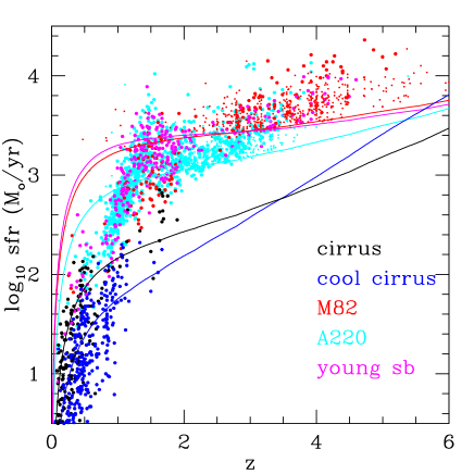
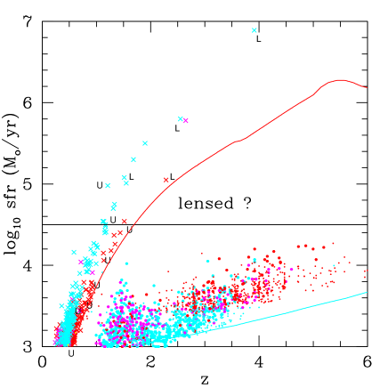
Figure 2: L: Star formation rate versus redshift for HerMES Lockman+XMM+ES1 galaxies, with loci showing 500 $\mu$m selection limits for each template type. Small dots are unidentified sources. R: Star-formation rate versus redshift for extreme starbursts from both HerMES (Lockman+XMM+ES1, filled circles) and from the IRAS RIFSCz catalogue (crosses). Known lenses are indicated by L and cases known to be unlensed indicated by U. The unlensed object apparently above the 30,000 $M_{\odot}/yr$ line (F14218+8345) is discussed in section 4. Typical 60 and 500 $\mu$m selection limits are indicated by the red and cyan loci.

5 Stellar mass, dust (and gas) mass, star formation rate

We derive stellar masses, dust & gas masses, and star formation rates for both the RIFSCz and HerMES sources by fitting model Spectral Energy Distributions (SEDs) to the catalogue data. Our approach of fitting optical and near infrared SEDs with templates based on stellar synthesis codes (Babbedge et al 2006, Rowan-Robinson et al 2008) allows us to estimate stellar masses. The templates are derived using simple stellar populations, each weighted by a different star formation rate and specified extinction (Berta et al 2004). An empirical correction is applied to allow for the variation of mass-to-light ratio with age (Rowan-Robinson et al 2008). A Salpeter mass-function is assumed.

Similarly, fitting mid infrared, far infrared and submillimetre data with templates based on radiative transfer models (Efstathiou et al 2000, 2003, Rowan-Robinson et al 2010, 2013, 2016), allows us to estimate star formation rates and dust masses.

Table 7: A comparison between our new star-formation rate density, and that previously published in Rowan-Robinson et al (2016).

Mean Redshift	0.5-1.0	1.0-1.5	1.5-2.0	2.0-2.5	2.5-3.0	3.0-3.5	3.5-4.0	4.0-4.5
Old SFRD ($\log_{10}(\phi)$)	-1.28$\pm$0.21	-0.95$\pm$0.11	-1.06$\pm$0.13	-1.05${}^{+0.27}_{-0.09}$	-0.82${}^{+0.18}_{-0.36}$	-0.99${}^{+0.29}_{-0.46}$	-0.82${}^{+0.18}_{-0.36}$	-0.79${}^{+0.14}_{-0.41}$
($M_{\odot}yr^{-1}Mpc^{-3}$)
New SFRD	-1.27$\pm$0.10	-0.93$\pm$0.11	-1.03$\pm$0.18	-0.90$\pm$0.08	-0.99${}^{+0.25}_{-0.07}$	-1.06$\pm$0.18	-0.89${}^{+0.21}_{-0.46}$	-0.85${}^{0.09}_{-0.58}$

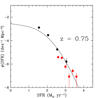
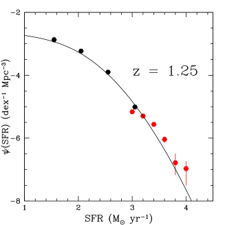
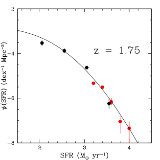
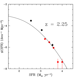
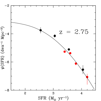
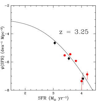
Figure 3: The revised star-formation rate functions for $z=0.25-3.25$, using a least-squares normalization at $24-500\,\mu$m. Black dots: data from Gruppioni et al (2013), red dots: present work.

In the automated fitting of infrared SED templates and calculation of infrared luminosities and other derived quantities, we previously normalised the SEDs at 8 $\mu$m, if the source was detected there, or at 24 $\mu$m otherwise. In studying the SEDs of galaxies with very high star-formation rates, we have found that normalisation at 8$\mu$m for sources at z = 1.5-3.5 can result in poor estimates of the infrared luminosity, because for many sources with z $>$ 1.5 the 8 $\mu$m emission is dominated by starlight. For z $>$ 3.5 we already required normalisation to be at 24 $\mu$m (for this reason).

We have therefore switched to normalisation (and luminosity estimation) based on a least-squares fit at 24-500$\mu$m for all sources. We have required a 24 $\mu$m detection in order to associate a Herschel source with a SWIRE photometric redshift catalogue source, so all sources have 24, 350 and 500 $\mu$m detections. This change significantly reduces the number of very high luminosity (and high star-formation rate) galaxies. From detailed SED modelling, we estimate the uncertainty in our corrected luminosities and star-formation rates as $\pm$0.1 dex. The star-formation rates are calculated for a 0.1-100 $M_{\odot}$ Salpeter IMF. Changing to a Miller-Scalo IMF would increase the star-formation rates by a factor 3.3, while changing the mass range to 1.6-100 $M_{\odot}$, ie forming A, B, O stars only, would reduce them by a factor 3.1 (Rowan-Robinson et al 1997).

Figure 2L shows our revised plot of star-formation rate (SFR) against redshift for HerMES-SWIRE galaxies, which can be compared with Fig 2L of Rowan-Robinson et al (2016). Details of the revised HerMES-SWIRE catalogue are given at http:$//$mattiavaccari.net$/$df$/$mrr$/$readmespirerev. The revised luminosities have some effect on the bright end of the star-formation rate functions. In figure 3 we show the star-formation rate functions for $z=0.75-3.25$, derived using the new least-squares normalisation. The tendency of the bright end of the function to be overestimated relative to the model fits (figure 9 of Rowan-Robinson et al 2016) has disappeared. The new parametric fits give star-formation rate densities that differ from the values of Rowan-Robinson et al (2016) by $<1\sigma$. A comparison between our SFRD and those previously reported is also given in Table 7. The effect on the derived star-formation-rate density from $z=0-6$ is negligible. For $z>4.5$ there is no change, but these SFRDs are based almost entirely on sources with no association with SWIRE galaxies and so are very uncertain.

Figure 2R shows the SFR against redshift for HerMES-SWIRE and RIFSCz galaxies with SFR $>1000M_{\odot}/yr$. Typical IRAS 60 $\mu$m and Herschel 500 $\mu$m detection limits are indicated. The highest star-formation rates significantly exceed the highest rates found by Weedman and Houck (2008) at 0 $<$ z $<$ 2.5. There appears to be a natural upper limit to the SFR of 30,000 $M_{\odot}/yr$. No HerMES-SWIRE galaxies are found above this value and the IRAS-FSS galaxies above this limit are probably gravitational lenses (see previous section and Table 5). This limit could represent an Eddington-type radiation pressure limit on the star-formation rate of the kind postulated by Elmegreen (1983), Scoville et al (2001), and Murray et al (2005). Scoville et al (2001) give a limit for $L/M_{*}$ of 500 $L_{\odot}/M_{\odot}$, which would translate to SFR $<10^{4.5}M_{\odot}/yr$ for $M_{*}<10^{11.5}M_{\odot}$.

We can use the dust mass as a proxy for gas mass, assuming a representative value for $M_{gas}/M_{dust}$. Magdis et al (2011) have summarised values of $M_{gas}/M_{dust}$ as a function of metallicity for local galaxies, and shown that a redshift 4 galaxy lies on the same relation, with $M_{gas}\sim 100M_{dust}$ (cf also Chen et al 2013). We use this ratio to estimate $M_{gas}$ and then compare this with our stellar mass estimates. Figure 4L illustrates the behaviour of the ($M_{gas})/M_{*}$ ratio as a function of redshift in the HerMES galaxy sample. For HerMES galaxies with z$>$1, $M_{gas}$ is comparable with $M_{stars}$, so these are very gas-rich galaxies (as noted by Rowan-Robinson et al 2010). Very high gas fractions have been found in galaxies with z $>$ 1 by Daddi et al (2010), Tacconi et al (2010, 2013), and Carrilli and Walter (2013). At low z, $100M_{dust}\sim 0.01-0.1M_{*}$ so these galaxies have already consumed most of their gas in star-formation.

Figure 4R shows $M_{*}/SFR$ as a function of redshift. It is apparent that the time to double the stellar mass at z = 3-5 is $\sim 10^{8}$ yrs. In some objects the gas-depletion time is as low as 1-3x$10^{7}$ yrs (cf Rowan-Robinson 2000, Carilli and Walter 2013). The Scoville et al (2001) Eddington limit quoted above translates to $M_{*}/SFR\sim 10^{7}$ yrs.

The picture that emerges is that the Herschel galaxies at z$>$3 are in the process of making most of the stars in the galaxy. Essentially these are metal factories. However we are not seeing monolithic galaxy formation of the kind postulated by Partridge and Peebles (1967), even though the star-formation rates and time-scales are similar to those they suggested, because we can see from the optical and near infrared SEDs that there has been an earlier generation of star-formation at least 1 Gyr prior to the star-formation we are witnessing. This is evidenced by the classic 0.4-2$\mu$m SED profile of evolved red giant stars seen in the SEDs of many of these galaxies (cf Fig 9 of Bruzual and Charlot 2003). Between z = 1 and the present epoch we see a dramatic decline in the gas content and star-formation rate. For z $<$0.5 the gas depletion time-scale is longer than the age of the universe so these are galaxies that must have had a much higher rate of star-formation in the past.

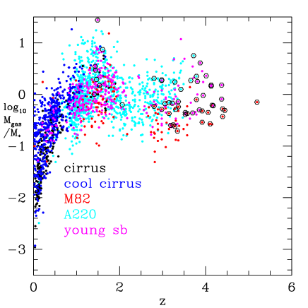
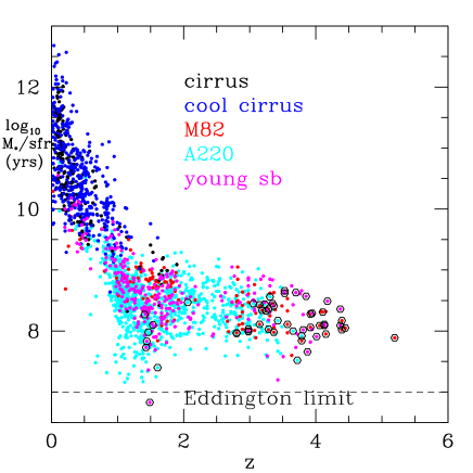
Figure 4: L: $M_{gas}/M_{*}$ vs. redshift (where $M_{gas}=100M_{dust}$). Circled points are the ‘extreme’ starbursts, those with SFR$>5000\,M_{\odot}yr^{-1}$. R: $M_{*}/SFR$ (or, the time-scale needed to make the observed mass of stars at the present star-formation rate) vs. redshift for HerMES galaxies. The source are labelled by their dominant infrared template type. The candidate extreme starbursts are shown circled.

6 Extreme starbursts

Here we look in more detail at the galaxies in the HerMES-SWIRE survey with implied star-formation rates greater than 5000 $M_{\odot}/yr$. Previously, detailed studies have been presented of just two objects in this class: Rowan-Robinson and Wang (2010) show the SED of one unlensed RIFSCz galaxy in this class (IRAS F15307+3252, z = 0.926) with SFR = 8100 $M_{\odot}yr^{-1}$, and Dowell et al report an object (FLS1, z = 4.29) with SFR = 9700 $M_{\odot}yr^{-1}$.

Our starting point is the HerMES-SWIRE (Lock+XMM+ES1) galaxies with SFR $>5000M_{\odot}yr^{-1}$, according to our automated infrared template fitting. There are 70 candidates in all (details given in Tables A1-A3), but we have taken a robust approach to the reliability of the redshift estimates, rejecting sources with lower-redshift aliases which give acceptable SED fits, and to the possibility of alternative associations with lower redshift counterparts or blends (see below), resulting in a final list of 38 reliable extreme starbursts. Details of the rejected sources and the reasons for rejection are given in Table A3. Sources from Table A3 have been excluded from Figs 4,11,12.

6.1 Reliability of redshift estimates

For the 70 candidate objects, we refine the redshift estimates adopting the approach of Rowan-Robinson et al (2016), who showed that fitting our starburst templates to the 250-350-500 $\mu$m data gives an effective estimate of submillimetre redshift, $z_{subm}$. Combining the $\chi^{2}$ distributions for the photometric and submillimetre redshifts gives a best fit combined redshift $z_{comb}$. The values of $z_{subm}$ and $z_{comb}$ are given in Tables A1 and A2. If $z_{comb}$ is significantly less than $z_{phot}$ and gives an acceptable SED fit, we have removed the object from the extreme starburst category and the SED is not shown here (17 objects in all). It is possible that in some cases the higher redshift is correct, but we prefer to err on the side of caution. The source 9.17274-43.34398 ($z_{phot}$ = 3.06) has a spectroscopic redshift of 1.748, which agrees well with $z_{subm}$, and so the source has been excluded.

We have also examined the $\chi^{2}$ distribution for the photometric redshift fit to see if any lower redshift aliases are present and the SEDs have also been examined for these aliases. Again we have erred on the side of caution and removed 7 objects with lower redshift aliases. 70 and 160 $\mu$m fluxes have been included in the SED plots only if they have a signal-to-noise ratio of at least 4. For three sources (35.73369-5.62305, 7.98209-43.29812 and 161.89894+58.16401), $z_{comb}$ is significantly less than $z_{phot}$, but the source remains in the extreme starburst category even with $z=z_{comb}$, so we have shown the SED with $z_{comb}$ above the corresponding SED for $z_{phot}$.

For 36.84426-5.31016 the photometric redshift (3.07) agreed well with the $z_{subm}$ (3.01) and with $z_{comb}$ (3.07), but the $\chi^{2}$ for the photometric redshift fit was very poor, and the template fit to the far infrared and submillimetre data was also poor, so we have preferred an alternative association with a SWIRE $z_{phot}$ = 1.49 galaxy, which gives a good overall fit to the SED, and so have excluded the object from the extreme starburst category. There are four other objects where detailed modelling of the SED gave solutions differing from the automated fit, which did not confirm them as extreme starbursts.

As a further check on our photometric redshifts we have fitted our extreme starburst sample using the CIGALE code (Noll et al 2009). For 12 of our objects this yielded a lower preferred redshift. For each of these cases we have examined their overall optical-to-submillimetre SED to see if this alternative redshift provides a plausible fit. One of these we had already omitted due to a lower redshift alias in the photometric redshift $\chi^{2}$ distribution and for one the lower redshift alias still yields a star-formation rate in the extreme category. For 2 objects the CIGALE redshift offered a plausible alternative fit to the overall SED and these have been excluded.

We should also consider the reliability of the associations of Spitzer 3.6-24$\mu$m sources with optical and near infrared counterparts. Confusion is not an issue at 24$\mu$m and the astrometric accuracy of the merged 3.6-24$\mu$m sources is $\pm$0.5 arcsec (Shupe et al 2007, Vaccari 2015). The average number of galaxies to i=25.5, the limit of associations considered here, is 0.014 per sq arcsec (Kashikawa et al 2004), so multiple associations of optical-nir galaxies with Spitzer sources are extremely rare.

Generally the SED fits for the remaining 38 sources are reliable and plausible, though only one is based on an optical spectroscopic redshift. Spectroscopic confirmation of the remaining objects would be highly desirable. Almost all of our objects with $z_{phot}>4$ have S350$>$S250, but it is worth noting that the range of $z_{subm}$ for our galaxies with $S250>S350>S500$ is 1.16-4.09, so the latter condition does not imply low redshift.

To summarise the reliability of our redshift estimates for the 38 extreme starbursts: 1 has a spectroscopic redshift (indicated by 4 decimal places in Tables A1), a further 2 have photometric redshift estimates $z\leq$1.5 determined from at least 6 photometric bands, so the rms uncertainty in (1+z) is $<4\%$ and the probability of a catastrophic outlier is $<3\%$ (Rowan-Robinson et al 2013). For the 35 remaining objects with 1.5 $<z_{phot}<$ 5.2, 10 of which are based on only 3 or 4 photometric bands, the photometric redshift estimates are more uncertain, but are in most cases reinforced by the estimates of $z_{subm}$. Rowan-Robinson et al (2016) found that the rms uncertainty in $(1+z_{comb})/(1+z_{spect})$ for 28 Herschel galaxies with spectroscopic redshifts is $\sim 21\%$. From the $\chi^{2}$ distributions for our photometric redshift estimates we have estimated the corresponding redshift uncertainty, and hence estimated the uncertainty in the star-formation estimate. For 35/38 objects the uncertainty is $\leq$0.1 dex. This uncertainty could mean that a few of the objects could move out of the extreme starburst category, probably balanced by others whose redshift has been underestimated, but our overall conclusions are unlikely to be significantly affected.

For comparison we have listed the 19 IRAS RIFSCz objects with $SFR>5000M_{\odot}yr^{-1}$ in Table 6 (excluding the objects listed in Table 5). We have modelled the SEDs of these objects individually (not shown here). 11 of the 19 objects have spectroscopic redshifts, so for these objects the redshift uncertainty is not a major issue. However the starburst component is usually fitted out to only 60 or 100 $\mu$m so the star-formation rates are uncertain by a factor of $\sim$2. It would be valuable to observe these galaxies at submillimetre wavelengths.

6.2 Source blending, reliability of SWIRE associations

Because we threshold at 5 $\sigma_{tot}$, where $\sigma_{tot}$ is the total noise including confusion noise, problems of source blending and confusion will be reduced (section 3). As a check of this, for each of our 500 $\mu$m sources we looked at any other possible associations with 24 $\mu$m SWIRE sources within our 20 arc sec search radius. For 18 of our 38 sources there was only one 24$\mu$m-detected SWIRE photometric redshift catalogue counterpart within our 20 arcsec search radius. For the remainder we have summed the predicted 500$\mu$m fluxes (based on template fitting to the SWIRE data) for all 24$\mu$m-detected counterparts within the search radius and estimated the fraction of the predicted flux provided by our selected association. For 34$/$38 sources this fraction is $\geq 90\%$ and for a further 2 sources it is in the range 80-90$\%$. The overwhelming majority of the alternative associations are unlikely to contribute significantly to the observed 500$\mu$m flux.

We looked at the SEDs of all the alternative associations to see whether any of these provided plausible SEDs when combined with our submillimetre sources. For 5 of our 38 sources there was a plausible alternative lower redshift association and these could be possible cases of misidentification or blending. These have been shown in Tables A1 and A2 in brackets. One of these sources (164.64154+58.09799) has a radio association (see below and Table 7) which strongly supports the higher redshift association (the radio position is 0.7 arcsec from high redshift position, 15 arcsec from lower redshift position). For two other sources (164.28366+58.43524 and 164.52054+58.30782) the separation of the lower-z 24 $\mu$m association from the Herschel position is much less than for the higher-z association (1.9 and 0.6 arcsec compared with 16.0 and 15.3 arcsec, respectively), so the lower-z association may be correct. For 160.50839+58.67179 the Herschel position is 4.1 arcsec from our $z_{phot}$=3.81 association, 6.9 arcsec from an alternative $z_{phot}$=1.08 association, while for 35.28232-4.1400 the Herschel position is 2.4 arcsec from our $z_{phot}$=3.28 association, 5.3 arcsec from an alternative $z_{phot}$=2.55 association, so either association is plausible. We have shown the SEDs of these 5 alternative associations in Figs 6-9.

One option would be to split the 500 $\mu$m (and associated 350 and 250 $\mu$m fluxes) equally between the two possible associations. If this is done 2 of the 5 objects move out of the extreme starburst category defined here. Thus source blending or misassociation is a relatively small problem in this sample.

Confirmation of the correctness of our SWIRE associations with the 250-350-500 $\mu$m sources can be found through radio maps of some of these sources. Table 8 lists 7 of the 38 extreme starbursts for which we have radio data. The positional offsets of the radio sources from the SWIRE (3.6-24 $\mu$m) positions are all $<$ 1-2 arcsec. We can also calculate the q-values for these sources, where q = $log_{10}(L_{FIR}/L(1.4GHz))$. These lie in the range 2.0-2.6, with a mean of 2.33, in good agreement with the values found for lower redshift Herschel galaxies by Ivison et al (2010) and with the mean value 2.34 found for IRAS galaxies (Yun et al 2001). We have also shown positional offsets for 1.2mm MAMBO observations of 161.75087+59.01883 by Lindner the al (2011) and for 850 $\mu$m observations of the same source by Geach et al (2017). Hill et al (2018) have observed the same source with the SMA interferometer and confirm that it is a single source. These fluxes are included in the SED of this source plotted in Fig 5. This is our best-case object, with a spectroscopic redshift (and $z_{subm}$ closely agreeing with this), radio confirmation of the SWIRE association and the radio estimate of the star-formation rate agreeing well with that from the submillimetre data (q=2.36).

It is worth commenting that the positional uncertainties of our 500 $\mu$m sample are greatly improved by requiring also $5-\sigma$ detections at 350 $\mu$m. In most cases ($39/44$) there is a detection at 250 $\mu$m as well and this is the position used, where available.

While we believe we have presented strong arguments for the reality of these Herschel extreme starbursts, especially those confirmed by radio observations both positionally and in the ratio of far-infrared to radio luminosities, it will be important to confirm the correctness of our SWIRE associations through ALMA and other submillimetre mapping, and through further radio mapping (e.g. by LOFAR, GMRT, MeerKAT and SKA). The correctness of our lensing candidates can be confirmed by HST and JWST mapping. For the IRAS extreme starbursts (Table 7) confusion and source blending are not an issue.

In the 2.9 deg² of the SWIRE-CDFS area (not used in this study), we find 8 extreme starbursts, consistent with the surface-density of 1.9 per sq deg found in Lockman+XMM+ES1. Unfortunately none of these lie in the 0.25 sq deg area surveyed at 870 $\mu$m with LABOCA by Weiss et al (2009), and followed up with ALMA by Hodge et al (2013).

6.3 Role of lensing

Although we believe we have removed all the lensed systems from our sample (section 4) we need to consider whether any of these 38 extreme starbursts could be lensed. From the analyses of Negrello et al (2010) and Wardlow et al (2013) it is the brightest 500 $\mu$m sources that are most likely to be lensed. None of our extreme starbursts have S500 $>$ 80 mJy but 6 have 60 $<$ S500 $<$ 80 mJy. Because there is reasonable agreement between $z_{phot}$ and $z_{subm}$ for these sources (exact agreement for 3 of the objects), they could only be lensed if the optical and submillimetre emission was also from the lensed galaxy. This would make them distinct from the known submillimetre lenses. Also 3 of these bright sources are amongst those confirmed by radio surveys (Table 7) and not reported as lensed. The lensing galaxy candidates found by Rowan-Robinson et al (2014) typically have i-magnitudes in the range 19-22, significantly brighter than the optical counterparts of our extreme starburst sample. We have also checked whether known clusters lie close to any of our 38 objects, in case cluster lensing was an issue, but have found none within one arcmin of our objects. Our expectation is that few or none of our 38 objects will turn out to be lensed systems.

Table 8: Radio positional offsets and q-values for extreme starbursts

RA(J2000)	Dec(J2000)	frequency	flux-density	offset	reference	q	$log_{10}$ SFR
				arcsec			($M_{\odot}yr^{-1}$)
36.10986	-4.45889	1.4GHz	0.219$\pm$0.026mJy	0.5	(2)	2.46	4.20
161.75087	59.01883	324.5MHz	687$\pm$72$\mu$Jy	0.7	(3)	2.36	3.75
		1.4GHz	278.8$\pm$15.2$\mu$Jy	1.2	(4)
		1.2mm	3.5$\pm$0.6mJy	1.5	(5)
		850$\mu$m	9.29$\pm$1.05mJy	1.4	(6)
161.98271	58.07477	1.4GHz	0.125mJy	1.1	(7)	2.12	3.76
162.33324	58.10657	1.4GHz	1.36mJy	1.1	(7)	2.45	3.73
162.46065	58.11701	1.4GHz	0.064mJy	1.7	(7)	2.50	3.88
162.91730	58.80596	324.5MHz	1013$\pm$96$\mu$Jy	1.6	(3)	2.47	3.75
		1.4GHz	0.504mJy	1.0	(7)
164.64154	58.09799	1.4GHz	0.182mJy	0.7	(7)	2.37	3.72

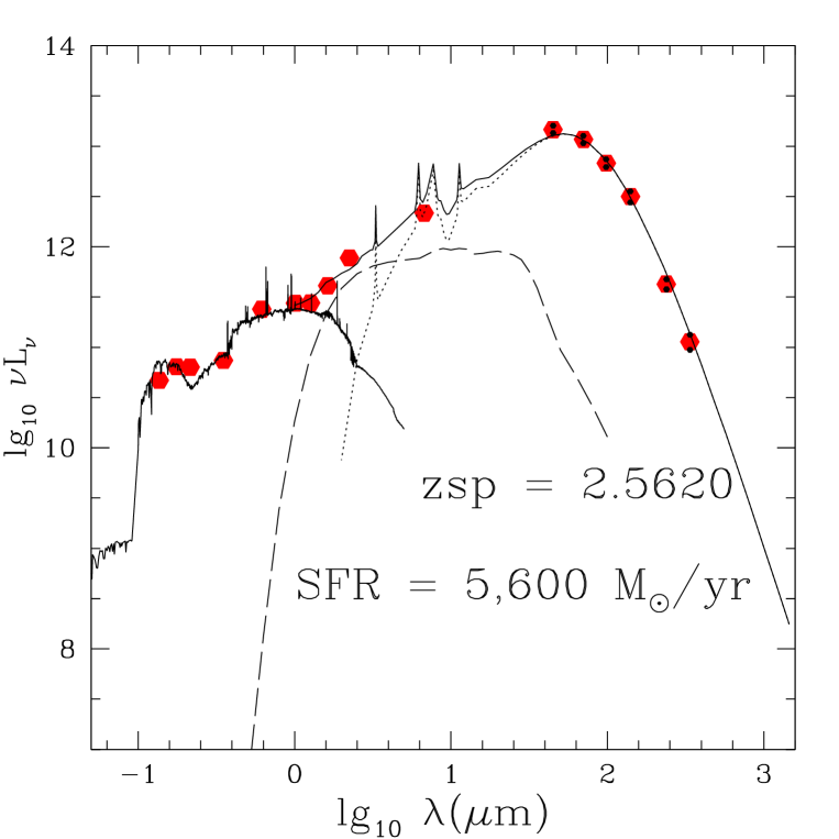
Figure 5: Rest-frame SED of 161.75087+59.01883, Herschel-SWIRE 500 $\mu$m source with spectroscopic redshift and extreme starburst luminosity. SWIRE association is confirmed by radio, 1.2mm, and 850 $\mu$m positions (latter two fluxes shown in SED). Errors for submillimetre fluxes indicated by black dots. Dotted loci: M82 starburst, long-dashed loci: AGN dust torus.

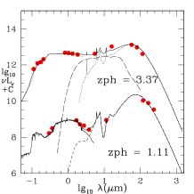
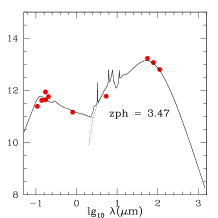
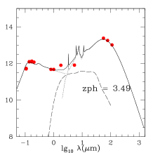
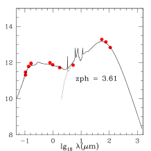
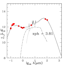
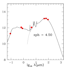
Figure 6: Rest-frame SEDs of Herschel-SWIRE 500 $\mu$m sources with extreme starburst luminosities (SFR$>5000\,M_{\odot}yr^{-1}$), labelled with the redshift, whose optical through near-infrared SEDs are best-fitted by a QSO template. Alternative SWIRE associations are shown plotted below the extreme starburst solution. Possible redshift aliases ($z_{comb}$)are shown plotted above the preferred $z_{phot}$ solution. Dotted loci: M82 starburst, dashed loci: Arp 220 starburst, long-dashed loci: AGN dust torus. The constant C = 0 except in cases where SEDs are shown for both the photometric redshift and for a lower redshift alternative SWIRE association. In these cases C = -2 for the lower SED and +1 for the upper one.

6.4 SEDs of extreme starbursts

We present SEDs for these extreme starbursts in the following figures. Figure 6 shows SEDs of extreme starbursts in the Herschel-SWIRE fields whose optical and near infrared data is fitted with a QSO template. Pitchford et al (2016) have studied a sample of 513 Type 1 QSOs detected by Herschel at 250 $\mu$m, some in the HerMES-SWIRE areas, and found star-formation rates ranging up to 5000 $M_{\odot}/yr$. In Figure 7 we show SEDs of objects whose optical-nir data is fitted with a galaxy template, but whose mid ir data show the presence of an AGN dust torus. These sources are plausibly Type 2 AGN whose host galaxies exhibit extreme rates of star formation. Of the 38 objects in our sample, 19 have optical through mid-infrared SEDs consistent with Type 1 or Type 2 AGN. In no case however does the luminosity of the AGN exceed that of the starburst.

In contrast, there exist many examples of ‘pure’ extreme starbursts in our sample. Figure 8 shows SEDs of objects whose optical and near infrared data are fitted with galaxy templates and whose mid ir, far ir and submillimetre data are fitted with M82 or Arp220 starburst templates. Figure 9 shows an especially interesting set of examples of pure extreme starbursts, whose infrared SEDs are best fit with young starburst templates. None of these objects show any evidence for significant AGN activity. Altogether 19$/$38 objects are pure starbursts.

As a check on our star-formation rate estimates we have also fitted the overall SEDs with the CIGALE code, using our preferred redshifts. We find that the CIGALE SFR estimates are in broad agreement with ours.

The star formation rates in these extreme starbursts all lie in the range $5,000-30,000\,M_{\odot}yr^{-1}$. As noted in the introduction, such high star formation rates are not predicted by any current semi-analytic model for galaxy formation, so these objects pose a serious challenge to theoretical models. Our 38 Herschel-SWIRE objects correspond to a surface density of 1.9 extreme starbursts per sq deg. The $500\,\mu$m sources which are not associated with SWIRE galaxies could add up to a further $\sim 9$ extreme starbursts per sq deg.

In Tables A1,A2 we have also shown our stellar mass estimates. They lie in the range $lg_{10}M_{*}$ = 11.28-12.50, so these are exceptionally massive galaxies. For 3.5$<z<$4.5, 11.5$<lg_{10}M_{*}<$12.5, there are 16 objects, yielding a space-density of $10^{-7.12}Mpc^{-3}dex^{-1}$, which fits nicely on an extrapolation of the mass-function given by Davidzon et al (2017, their Figs 8,11).

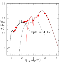
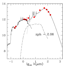
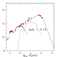
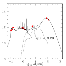
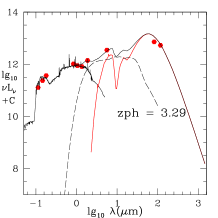
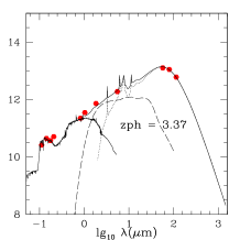
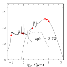
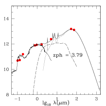
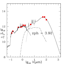
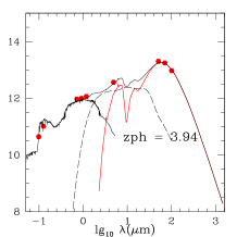
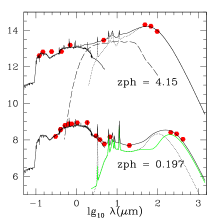
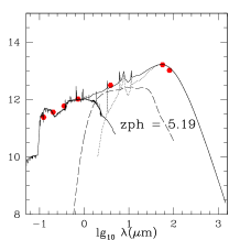
Figure 7: Rest-frame SEDs of it Herschel-SWIRE 500 $\mu$m sources with extreme starburst luminosities, labelled with the redshift, whose optical through near-infrared SEDs are best-fitted by a galaxy template, but whose mid-infrared SEDs require an AGN dust torus template. Red loci: young starburst template, other details as in Figure 6.

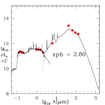
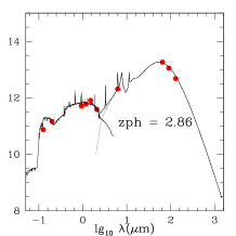
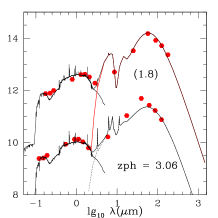
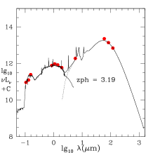
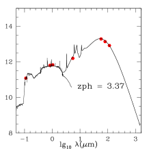
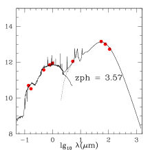
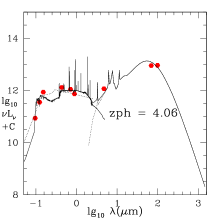
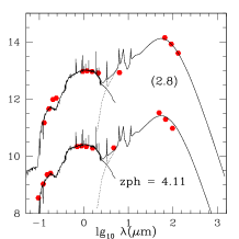
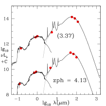
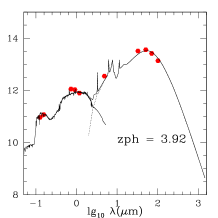
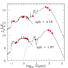
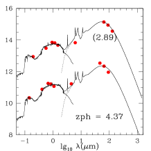
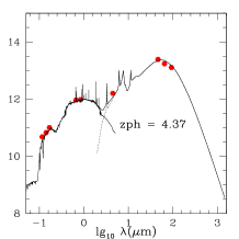
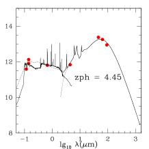
Figure 8: The rest-frame SEDs of Herschel-SWIRE 500 $\mu$m sources with extreme starburst luminosities, labelled by redshift, whose optical through near-infrared SEDs are best-fitted by a galaxy template, and whose mid- through far-infrared SEDs are fitted with M82 or Arp220 starburst templates. Other details are the same as in Figure 6.

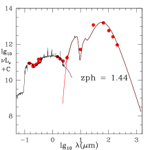
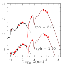
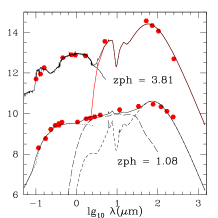
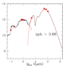
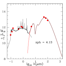
Figure 9: The SEDs of it Herschel-SWIRE 500 $\mu$m sources with extreme starburst luminosities, labelled by redshift, whose optical through near-infrared SEDs are best-fitted by a galaxy template, and whose mid- through far-infrared SEDs are fitted with young starburst templates. Red loci: young starburst template. Other details are the same as in Figure 6.

7 Role of AGN

A surprisingly high proportion of Herschel extreme starbursts have an inferred AGN dust torus component (50$\%$). The dust tori are, however, quite weak and in no case does $L_{tor}$ exceed $L_{sb}$, nor does the dust torus contribute significantly to the submillimetre emission. We can use the ratio of luminosity in the dust torus to that in the bolometric uv-optical-nir luminosity of the QSO, $L_{tor}/L_{bh}$, as a measure of the covering factor by dust, f, which is independent of the geometry of the dust, assuming the thermal uv-optical-nir emission from the accretion disk is radiated isotropically. In the case of a toroidal dust distribution, f would be a measure of the opening angle of the torus. Figure 10 shows $L_{tor}/L_{opt}$ versus redshift for SWIRE QSOs, where $L_{opt}$ is the 0.1-2$\mu$m luminosity of the QSO. Assuming the bolometric output of the black hole, $L_{bh}=2.0L_{opt}$ (Rowan-Robinson et al 2009), the average covering factor, f, is $\sim$0.4 for z$>$2, declining to $\sim$0.16 at z = 0. This trend can also be interpreted as a decline in dust torus covering factor with declining optical (and bolometric) luminosity (see Rowan-Robinson et al 2009 and references quoted therein).

Using this relation, Fig 11L shows black-hole mass, $M_{bh}\beta^{-1}$, versus total stellar mass, $M_{*}$, for Herschel galaxies and for IRAS-FSS galaxies with z $<$ 0.3, where $M_{bh}$ is estimated from $L_{bh}$ assuming that the AGN is radiating at a fraction $\beta$ of the Eddington luminosity:

$$L_{bh}=\beta L_{Edd}=4\pi\beta GM_{bh}m_{p}c/\sigma_{T}$ = 3.2 x $10^{4}\beta(M_{bh}/M_{\odot})(L_{\odot})$$ (6)

$L_{bh}$ is estimated as 2.0 $L_{opt}$ for QSOs, and from $L_{tor}/f$ for galaxies with AGN dust tori. A wide range of values of the Eddington ratio $\beta$ is found in the literature (Babic et al 2007, Fabian et al 2008, Steinhardt and Elvis 2009, Schutze and Wistotzki 2010, Suh et al 2015, Pitchford et al 2016, Harris et al 2016), with a typical range of 0.01-1 for z $>$ 1 (Kelly et al 2010, Lusso et al 2012). Since QSOs are excluded from Fig 11L by the requirement for a measurement of stellar mass, these are all Type 2 AGN. The mean value of $lg_{10}L_{bh}/(\beta M_{*})$ for 500 HerMES-SWIRE AGN is -4.11, with an rms dispersion of 0.56. There will be a contribution to this rms from the dispersion in values of the covering factor f. The distribution of AGN in Fig 11L is broadly similar to the equivalent plot by Reines and Volonteri (2015) for broad-line AGN, though we have a higher proportion of high mass galaxies and we do not have objects corresponding to their elliptical and S0 galaxies.

Figure 11R shows $M_{bh}\beta^{-1}/M_{*}$ versus redshift for the same galaxies. If we take $\beta\sim$ 0.1 as a characteristic value, then $M_{bh}/M_{*}\sim 0.001$ at all redshifts, with a range of $\sim\pm$ 1 dex. This is reminiscent of the Magorrian et al (1998) relation between black-hole mass and bulge mass (see also review by Kormendy and Ho 2013). This ratio is set by the very high star-formation (and black-hole build-up) at redshift 2-5. The Milky Way, with $M_{*}=6\times 10^{10}M_{\odot}$ and $M_{bh}=4\times 10^{6}M_{\odot}$ lies on the lower end of this range.

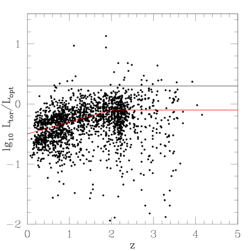
Figure 10: The behaviour of the torus covering factor ($L_{tor}/L_{opt}$) as a function of redshift for the HerMES extreme starbursts with QSO-like optical SEDs. The solid black line corresponds to $L_{tor}=L_{bh}$ with an assumed optical bolometric correction of 2.0 (Rowan-Robinson et al 2009). The red line shows a relation that approximately reproduces the trend seen among the plotted population.

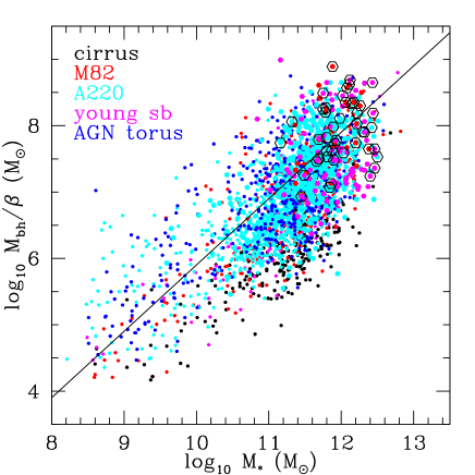
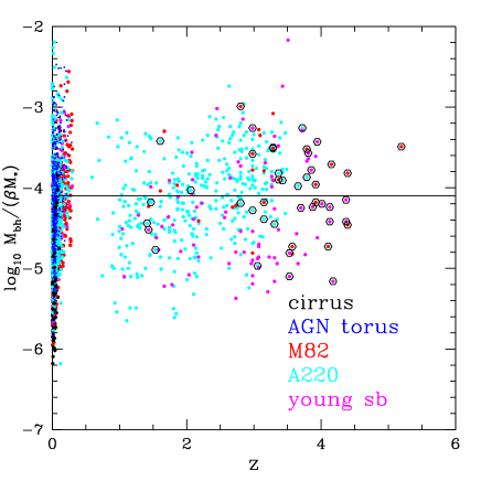
Figure 11: L: Black-hole mass, $M_{bh}\beta^{-1}(M_{\odot})$, versus total stellar mass, $M_{*}(M_{\odot})$, for HerMES-SWIRE sources and for RIFSCz sources with z$<$0.3 (smaller points), with AGN dust tori. QSOs are excluded by the requirement that there be a stellar mass estimate, so these are all Type 2 AGN. Circled points are Herschel extreme starbursts. R: $M_{bh}/(\beta M_{*})$ versus z for HerMES-SWIRE sources and for RIFSCz sources with z$<$0.3, with AGN dust tori.

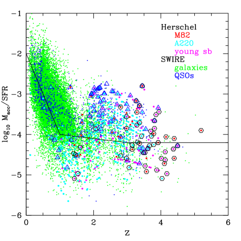
Figure 12: $log_{10}M_{acc}/SFR$ versus z for SWIRE (small green and blue dots) and HerMES sources (larger red cyan and magenta dots). Circled points are extreme starbursts and blue open triangles denote HerMES QSOs.

Figure 12 shows $M_{acc}/SFR$ versus redshift for Herschel galaxies and for (non-Herschel) SWIRE galaxies (smaller symbols), where the black-hole accretion rate $M_{acc}$ is calculated assuming conversion efficiency of accreting mass to radiation is $\epsilon$=0.1:

$$L_{bh}=\epsilon{M_{acc}}c^{2}$$ (7)

Note that the combination of equations (6) and (7) gives the Salpeter time-scale for black hole growth $t_{S}=4.10^{8}\epsilon\beta^{-1}$ yrs (Salpeter 1964). QSOs have been indicated in Fig 11 by open blue triangles.

Figure 12 shows that $M_{acc}/SFR$ is $\sim 10^{-4}$ at z = 2-5, but that this ratio has increased by a factor of 30 by z $<$0.5. The star-formation rates in $z<0.5$ galaxies are 1000 times lower than those seen in the extreme starbursts, but the black hole accretion rates are only 30 times lower. This is consistent with source count models that find shallower evolution for AGN compared to that for starbursts (e.g. Rowan-Robinson 2009). A recent apparent exception to this has been presented by Barnett et al (2015), who quote a much higher value of $M_{acc}/SFR\sim$ 0.2 for a redshift 7.1 QSO, based on a SFR derived from the CII 158 $\mu$m line. However they also quote a bolometric luminosity of $6.7\times 10^{13}L_{\odot}$, which could yield a SFR of $\sim$ 13,000 $M_{\odot}/yr$, about 100 times their estimate from CII. This would move $M_{acc}/SFR$ into the range seen in Fig 12.

Figure 12 shows that there is an intimate and evolving connection between black hole accretion and star formation. A plausible interpretation of this result is as follows. In these high redshift, high luminosity submillimetre galaxies we are seeing major mergers (Chakrabarti et al 2008, Hopkins et al 2010, Haywards et al 2011, Ivison et al 2012, Aguirre et al 2013, Wiklind et al 2014, Chen et al 2015), in which the star formation is taking place close to ($<\,$ 1 kpc) the galactic nucleus, so it is not surprising that there is a strong connection between star-formation and black-hole growth. However at recent epochs ($z<1$) star-formation is mainly fed by accretion from the cosmic web, by minor mergers and interactions, and by spiral density waves, so is taking place further from the galactic nucleus. This uncouples the direct connection between star-formation and black-hole growth. The gas feeding the black hole is fed to the galactic nucleus more gradually and may include gas fed by mass-loss from stars. It is however still surprising that it is so much easier to feed a black hole at the present epoch than it is to form stars. Another possible interpretation of Fig 12 is that the emission from the AGN provides a limit to star-formation, forcing $SFR<10^{5}M_{acc}$.

It is possible that the high proportion of AGN amongst these extreme starbursts is pointing to the influence of AGN jet-induced star formation in these extreme objects (Klamer et al. 2004; Clements et al. 2009). While we currently have no information on the prevalence of jets in the sample discussed here, there are individual extreme starbursts such as J160705.16+533558.5 (Clements et al., 2009, and in prep) and 4C41.17 (de Breuck et al., 2005; Steinbring, 2014) where there are strong indications that jets are triggering star formation. Furthermore, Klamer et al. (2004) presents a sample of 12 z$>$3 star forming AGN where star formation appears to be triggered by relativistic jets. More information on the AGN and gas distribution in the sources in the current paper is clearly needed, but we note that the time-scales for these starbursts and the time-scale for black hole growth are remarkably well matched at $\sim$ 10⁷ years (Rigopoulou et al. 2009). However, the greatly enhanced gas supply to the nucleus associated with violent mergers may be a sufficient explanation.

If there is a connection between black hole accretion and star-formation, why do only half of our extreme starbursts harbour AGN ? Firstly the non-detection of an AGN dust torus sets only a modest upper limit on $M_{bh}\beta^{-1}/M_{*}$ of $\sim 10^{-5}$, i.e. at the lower end of the observed distribution. It is possible that there is a phase-lag between star-formation and black-hole growth and this is supported by the fact that of the 11 galaxies fitted with a young starburst template in the infrared only two also have an AGN dust torus. To grow a black hole there has to be a black hole present in the first place and perhaps some galaxies have not yet formed a massive nuclear black hole.

Finally, we note an interesting disconnection between X-ray detected AGN, and the Herschel sources. The SWIRE-Lockman area includes the CLASX X-ray survey. Rowan-Robinson et al (2009) gave a detailed discussion of the associations of CLASX and SWIRE sources. Only two of the 400 CLASX-SWIRE sources are detected by Herschel-SPIRE. This is consistent with the idea that, while AGN are present in the Herschel submillimetre galaxy population, they make a negligible contribution to the submillimetre flux.

8 Conclusions

After careful exclusion of lensed galaxies and blazers, we have identified samples of extreme starbursts, with star-formation rates in the range 5000-30,000 $M_{\odot}/yr$, from the IRAS-FSS 60 $\mu$m galaxy catalogue (RIFSCz) and from the Herschel-SWIRE (HerMES) 500 $\mu$m survey. The correctness of our SWIRE associations is confirmed for 8 objects by radio maps. ALMA submillimetre mapping and deeper radio mapping by LOFAR, GMRT, MeerKAT and SKA will help confirm the reality of the remaining sources.

There do not seem to be any genuine cases with SFR$>$30,000 $M_{\odot}/yr$ and this may be essentially an Eddington-type limit. The SEDs of 38 HerMES extreme starbursts have been modelled in detail. The photometric redshifts are, in almost all cases, supported by redshift estimates from the 250-500 $\mu$m colours. The proportion of 500 $\mu$m sources which may be subject to blending or association with the wrong 24 $\mu$m source is $<12\%$. Using dust mass as a proxy for gas mass, extreme starbursts are found to be very gas rich systems, which will double their stellar mass in 0.3-3 x $10^{8}$ yrs.

About half of the Herschel extreme starburst systems also contain an AGN, but in no case do these dominate the bolometric output. With assumptions about the Eddington ratio and accretion efficiency, we find a universal relation between black-hole mass and total stellar mass, with $M_{bh}\sim 0.001M_{*}$. This is driven by the episode of extreme star-formation and black hole growth at z=2-5. However while the star formation rate has fallen by a factor of 1000 between redshift 5 and the present epoch, the black hole accretion rate has fallen by a factor of only 30, suggesting a decoupling between star formation and the feeding of the nuclear black hole.

Appendix A Tabulated data for Extreme Starbursts

Tables from section 6.

Table 9: Extreme starbursts: QSOs and Type 2 AGN

RA	Dec	$m_{i}$	S24	S250	S350	S500	$z_{phot}$	type	$\chi^{2}$	$n_{b}$	$z_{subm}$	$z_{comb}$	$M_{*}$	SFR
			($\mu$Jy)	(mJy)	(mJy)	(mJy)							$\log(M_{\odot})$	$\log(M_{\odot}yr^{-1})$
QSOs, Fig 6
164.64154	58.09799	20.95	1386.3	44.9	45.4	28.0	3.37	QSO	2.1	11	2.01	3.07		3.71
(164.64879	58.09513						1.11							2.74)
162.77605	58.52327	22.32	184.6	54.5	53.0	41.1	3.47	QSO	3.2	8	3.19	3.37		3.71
161.85410	57.91928	21.11	245.8	76.1	80.3	65.3	3.49	QSO	1.3	10	3.42	3.47		3.86
162.20728	58.28162	21.59	205.5	56.6	57.7	40.3	3.61	QSO	8.5	10	3.14	3.37		3.83
161.36092	58.03157	20.67	428.6	-	37.5	41.2	3.81	QSO	5.2	11	5.05	3.90		3.83
162.68120	57.55606	g=24.35	194.9	25.5	37.0	38.3	4.50	QSO	1.3	3	4.79	4.50		3.79
Type 2 AGN, Fig 7
33.71100	-4.17344	22.53	1016.3	96.2	69.0	32.5	1.47	Scd	9.3	6	1.92	1.57	11.80	3.81
162.91730	58.80596	22.03	1964.8	183.8	133.1	78.7	2.06	Sab	45.6	6	2.11	2.09	12.22	3.81
161.75087	59.01883	23.66	1329.6	75.0	61.0	40.6	2.5620	Scd	1.7	7	2.53		11.78	3.70
35.95578	-5.08144	23.85	1002.1	71.2	77.6	59.5	3.15	Sab	7.3	5	3.32	3.27	11.91	3.80
10.23271	-44.07592	R=21.50	487.0	75.3	68.1	45.7	3.29	sb	13.3	5	2.67	3.07	11.75	3.77
160.33716	59.40493	22.36	1225.7	-	36.8	39.0	3.29	Scd	6.7	6	4.93	3.27	12.08	3.71
36.15258	-5.10250	24.92	627.2	43.5	53.7	41.5	3.37	Sab	2.0	5	3.60	3.47	11.69	3.71
159.78395	58.55888	g=24.41	231.6	35.3	39.9	36.7	3.72	Sdm	0.0	3	3.91	3.68	11.32	3.79
36.96840	-5.02193	24.92	610.3	40.4	47.8	39.3	3.79	Sab	7.5	6	3.66	3.79	11.79	3.94
160.85139	58.02007	23.22	443.7	43.1	61.2	37.4	3.92	Sbc	2.6	5	2.24	3.37	12.21	3.94
35.92307	-4.73225	25.55	849.5	48.5	59.5	45.3	3.94	Sab	2.9	5	3.56	3.57	12.12	3.83
164.28366	58.43524	22.30	596.0	43.5	51.0	37.4	4.15	Scd	60.0	5	2.46	3.79	12.06	4.14
(164.28227	58.43064						0.20							0.40)
161.63013	59.17688	23.94	391.4	-	29.6	27.0	5.19	Scd	4.8	4	3.05	4.75	12.11	4.22

Table 10: Extreme starbursts: young starbursts, M82 and A220 type starbursts

RA	dec	i	S24	S250	S350	S500	$z_{phot}$	type	$\chi^{2}$	$n_{bands}$	$z_{subm}$	$z_{comb}$	$M_{*}$	SFR
			($\mu$Jy)	(mJy)	(mJy)	(mJy)							$\log(M_{\odot})$	$\log(M_{\odot}yr^{-1})$
young sbs,	Fig 9
159.03456	58.44533	21.37	1127.8	131.6	84.2	42.2	1.44	Scd	4.8	4	1.16	1.19	11.62	3.89
35.28232	-4.14900	g=25.31	636.1	53.7	58.3	55.1	3.27	Sab	2.4	4	3.84	2.80	11.28	3.70
(35.28037	-4.14839						2.55							3.59)
160.50839	58.67179	23.49	904.6	95.7	79.5	60.5	3.81	Sab	4.1	6	2.86	3.07	12.02	3.99
(160.51041	58.67371						1.08							3.05)
36.59817	-4.56164	25.11	389.5	59.3	67.2	54.7	3.88	Sab	2.1	5	3.53	3.68	11.49	3.85
161.98271	58.07477	22.10	264.4	44.2	45.3	33.6	4.13	sb	25.4	6	3.15	3.68	11.87	3.76
M82, A220 sbs,	Fig 8
162.33324	58.10657	22.61	516.4	56.9	52.9	59.6	2.80	Scd	6.1	8	4.09	2.89	11.69	3.72
9.64405	-44.36636	23.02	987.2	91.7	79.4	48.1	2.85	Scd	1.8	4	2.43	2.72	11.89	3.70
160.91940	57.91475	22.32	682.3	116.5	102.0	65.4	3.06	Sab	20.5	6	2.56	2.80	12.50	4.12
8.81979	-42.69724	R=22.90	706.2	87.4	74.6	53.9	3.19	Scd	6.1	5	2.72	2.98	12.06	3.79
162.38754	57.70547	g=24.13	519.3	65.7	65.0	56.3	3.37	Scd	1.6	3	3.47	3.37	12.15	3.74
36.71948	-3.96377	25.18	322.8	43.4	42.8	32.1	3.57	Sbc	5.2	5	3.10	3.27	12.21	3.70
162.46065	58.11701	21.96	252.5	-	28.4	41.4	4.06	sb (QSO?)	7.9	6	4.81	4.13	11.97	3.98
35.73369	-5.62305	23.42	422.0	73.1	60.9	42.1	4.11	Sbc	4.1	6	2.61	2.80	12.38	4.10
							2.80	Sbc						3.70
7.98209	-43.29812	R=24.87	275.8	45.6	49.7	38.8	4.13	Sab	0.02	3	3.37	3.37	11.90	3.82
							3.37	Sab						3.70
36.10986	-4.45889	24.59	828.6	88.4	89.5	67.0	3.92	Sab	2.0	5	3.14	3.27	12.26	4.21
164.52054	58.30782	23.40	306.9	81.9	92.1	58.2	4.18	Sab	0.03	3	2.16	3.07	12.40	3.99
(164.52888	58.30814						1.87							3.35)
161.89894	58.16401	23.60	315.0	66.4	59.7	35.3	4.37	Sab	22.7	4	1.82	2.89	12.32	3.97
							2.89	Sab						3.70
36.65871	-4.14628	24.91	288.8	46.1	45.7	48.1	4.40	Sbc	2.1	6	3.92	4.01	12.20	4.03
162.42290	57.18750	22.25	121.0	43.5	46.1	32.6	4.45	sb (QSO?)	5.6	4	3.22	4.37	11.79	3.78

Table 11: Rejected extreme starburst candidates

RA	dec	$z_{phot}$	type	$\chi^{2}$	$n_{bands}$	$z_{subm}$	$z_{comb}$	reason for rejection
159.24428	57.85775	3.06	Scd	3.1	5	1.80	1.51	$z_{comb}$ = 1.51 gives acceptable fit
35.49809	-5.92264	3.13	Sab	1.9	6	2.49	1.69	$z_{comb}$ = 1.69 gives acceptable fit
161.21138	58.11261	3.33	Sbc	26.8	5	2.02	1.75	$z_{comb}$ = 1.75 gives acceptable fit
162.55945	57.19608	3.70	sb	3.6	5	2.01	1.19	$z_{comb}$ = 1.19 gives acceptable fit
159.67438	58.55686	3.72	Scd	0.0	3	2.68	2.02	$z_{comb}$ = 2.02 gives acceptable fit
162.52769	57.28142	3.92	QSO	8.4	8	1.93	1.95	$z_{comb}$ = 1.95 gives acceptable fit
35.11967	-5.73062	3.94	Sbc	14.8	6	2.90	1.69	$z_{comb}$ = 1.69 gives acceptable fit
34.26031	-4.95556	4.15	Sbc	3.9	4	2.03	2.16	$z_{comb}$ = 2.16 gives acceptable fit
164.02647	52.07153	4.18	sb	2.5	4	2.74	1.82	$z_{comb}$ = 1.82 gives acceptable fit
9.28433	-44.23750	4.18	Scd	0.03	3	2.40	2.39	$z_{comb}$ = 2.39 gives acceptable fit
9.08571	-42.59628	4.25	Scd	0.85	3	2.33	2.09	$z_{comb}$ = 2.09 gives acceptable fit
36.25277	-5.59534	4.27	Scd	1.2	5	2.65	1.95	$z_{comb}$ = 1.95 gives acceptable fit
9.11142	-42.84052	4.60	Scd	0.03	3	2.36	2.31	$z_{comb}$ = 2.31 gives acceptable fit
9.30474	-43.03506	4.86	Scd	0.09	3	2.87	2.80	$z_{comb}$ = 2.80 gives acceptable fit
161.58835	59.65826	5.05	Scd	4.7	5	3.03	2.98	$z_{comb}$ = 2.98 gives acceptable fit
34.53469	-5.00769	4.40	sb	4.0	5	3.18	3.17	$z_{comb}$ = 3.17 gives acceptable fit
8.70199	-44.48560	4.73	Scd	0.01	3	3.45	3.47	$z_{comb}$ = 3.47 gives acceptable fit
9.17274	-43.34398	3.06	Sab	15.7	6	1.84	2.47	$z_{spect}$ = 1.748 (Bongiorno et al 2014)
35.73605	-4.88950	4.37	Scd	11.4	6	3.69	2.55	alias at $z_{phot}$ = 1.9 gives acceptable fit
35.33492	-5.74307	3.81	Sbc	2.7	4	2.06	2.09	alias at $z_{phot}$ = 1.7 gives acceptable fit
164.55716	58.65286	3.92	sb	2.3	6	2.96	3.57	alias at $z_{phot}$ = 1.2 fits 24-500$\mu$m
9.19681	-44.42382	5.00	sb (QSO?)	0.04	3	3.89	4.13	alias at $z_{phot}$ = 1.7 gives acceptable fit
159.95905	57.18814	3.37	Scd	0.1	3	4.88	3.37	alias at $z_{phot}$ = 1.95 gives acceptable fit
163.98088	57.81277	3.74	Scd	4.4	5	5.03	3.68	alias at $z_{phot}$ = 2.3 gives acceptable fit
162.84616	58.00514	4.01	sb	13.0	5	3.56	4.01	alias at $z_{phot}$ = 2.1 gives acceptable fit
160.16505	57.27072	3.70	Sab	31.2	4	3.45	3.68	CIGALE alias at $z_{phot}$ = 1.9 gives acceptable fit
162.26817	58.46461	3.15	Sbc	5.0	6	3.16	3.17	CIGALE alias at $z_{phot}$ = 1.7 gives acceptable fit
36.84426	-5.31016	3.07	QSO	42.1	14	3.01	3.07	alternative SWIRE association with $z{phot}$ = 1.49 fits better
9.62462	-43.74844	1.5670	QSO	2.9	9	2.40		SED fit implies SFR $<$ 3.70
164.96553	58.30081	2.3350	QSO	13.6	11	2.33		SED fit implies SFR $<$ 3.70
8.04056	-43.71930	1.51	Sab	26.4	7	2.96	2.09	SED fit implies SFR $<$ 3.70
35.11776	-5.50099	1.55	Scd	9.0	7	2.74	2.02	SED fit implies SFR $<$ 3.70