A Special Homotopy Continuation Method For A Class of Polynomial Systems

Abstract

A special homotopy continuation method, as a combination of the polyhedral homotopy and the linear product homotopy, is proposed for computing all the isolated solutions to a special class of polynomial systems. The root number bound of this method is between the total degree bound and the mixed volume bound and can be easily computed. The new algorithm has been implemented as a program called LPH using C++. Our experiments show its efficiency compared to the polyhedral or other homotopies on such systems. As an application, the algorithm can be used to find witness points on each connected component of a real variety.

1 Introduction

In many applications in science, engineering, and economics, solving systems of polynomial equations has been a subject of great importance. The homotopy continuation method was developed in 1970s [1][2] and has been greatly expanded and developed by many reseachers (see for example [3][4][5][6][7]). Nowadays, homotopy continuation method has become one of the most reliable and efficient classes of numerical methods for finding the isolated solutions to a polynomial system and the so-called numerical algebraic geometry based on homotopy continuation method has been a blossoming area. There are many famous software packages implementing different homotopy methods, including Bertini[8], Hom4PS-2.0[9], HOMPACK[10], PHCpack[11], etc.

Classical homotopy methods compute solutions in complex spaces, while in applications, it is quite common that only real solutions have physical meaning. Computing real roots of an algebraic system is a difficult and fundamental problem in real algebraic geometry. In the field of symbolic computation, there are some famous algorithms dealing with this problem. The cylindrical algebraic decomposition algorithm [12] is the first complete algorithm which has been implemented and used successfully to solve many real problems. However, in the worst case, its complexity is of doubly exponential in the number of variables. Based on the ideas of Seidenberg [13] and others, some algorithms for computing at least one point on each connected component of an real algebraic set were proposed through developing the formulation of critical points and the notion of polar varieties, see [14][15][16] and references therein. The idea behind is studying an objective function (or map) that reaches at least one local extremum on each connected component of a real algebraic set. For example, the function of square of the Euclidean distance to a randomly chosen point was used in [17][18]. On the other hand, some homotopy based algorithms for real solving have been proposed in [19][20][21][22][23][24]. For example, in [23], a numerical homotopy method to find the extremum of Euclidean distance to a point as the objective function was presented. More recently, the Euclidean distance to a plane was proposed as a linear objective function in [25].

In this paper, we follow the work of [25][26] to extend complex homotopy methods to finding witness points on the irreducible components of real varieties. To obtain such witness points, we first need to solve a special class of polynomial systems. Combining the polyhedral homotopy and the linear product homotopy, we give a special homotopy method for solving the system of that type. The root number bound of this method is not only easy to compute but also much smaller than the total degree bound and close to the BKK bound [27] when the polynomials defining the algebraic set is not very sparse. This key observation enables us to design an efficient homotopy procedure to obtain critical points numerically. The ideas and algorithms we proposed in this article avoid a great number of divergent paths to track compared with the total degree homotopy and save the great time cost for mixed volume computation compared with the polyhedral homotopy. The new algorithm has been implemented as a program called LPH using C++. Our experiments show its efficiency compared to the polyhedral or other homotopies on such systems.

The rest of this paper is organized as follows. Section 2 describes some preliminary concepts and results. Section 3 introduces a special type of polynomial systems we are considering. The new homotopy for these polynomial systems is also presented. It naturally leads to an algorithm which is described in Section 4. Based on this algorithm, in Section 5, we present a method to find real witness points of positive dimensional varieties, together with an illustrative example. The experimental performance of the software package LPH, which is an implementation of the method in C++, is given in Section 6.

2 Preliminary

2.1 Algebraic Sets and Genericity

For a polynomial system $f:{\bbbc^{n}}\to{\bbbc^{k}}$, let $V(f)=\{x\in{\bbbc^{n}}|f(x)=0\}$ and ${V_{\bbbr}}(f)=V(f)\cap{\bbbr^{n}}=\{x\in{\bbbr^{n}}|f(x)=0\}$ be the set of complex solutions and the set of real solutions of $f(x)=0$, respectively. A set $X\subset{\bbbc^{n}}$ is called an algebraic set if $X=V(g)$, for some polynomial system $g$.

An algebraic set $X$ is irreducible if there does not exist a decomposition ${X_{1}}\cup{X_{2}}=X$ with ${X_{1}},{X_{2}}\neq X$ of $X$ as a union of two strict algebraic subsets. An algebraic set is reducible, if there exist such decomposition. For example, the algebraic set $V(xy)\subset{\bbbc^{2}}$ is consisting of the two coordinate axes, and is obviously the union of $V(x)$ and $V(y)$, hence reducible.

For an irreducible algebraic set $X$, the subset of smooth (or manifold) points ${X_{reg}}$ is dense, open and path connected (up to the Zariski topology) in $X$. The dimension of an irreducible algebraic set $X$ is the dimension of ${X_{reg}}$ as a complex manifold.

Let $\mathcal{J}_{f}(x)$ denote the $n\times k$ Jacobian matrix of $f$ evaluated at $x$. By the Implicit Function Theorem, for an irreducible algebraic set $X$ defined by a reduced system $f$, $x\in{X_{reg}}\Leftrightarrow\mathrm{rank}(\mathcal{J}_{f}(x))=n-\dim X$. When $n=k$, the system $f$ is said to be a square system. In this case, a point $x\in V(f)$ is nonsingular if $\det(\mathcal{J}_{f}(x))\neq 0$, and singular otherwise.

On irreducible algebraic set, we can define the notion of genericity, adapted from[6].

Definition 1

Let $X$ be an irreducible algebraic set. Property P holds generically on $X$, if the set of points in $X$ that do not satisfy property P are contained in a proper algebraic subset $Y$ of $X$. The points in $Y$ are called nongeneric points, and their complements $X\backslash Y$ are called generic points.

Remark 1

From the definition, one sees that the notion of generic is only meaningful in the context of property P in question.

Every algebraic set $X$ has a (uniquely up to reordering) expression $X={X_{1}}\cup\ldots\cup{X_{r}}$ with ${X_{i}}$ irreducible and ${X_{i}}\not\subset{X_{j}}$ for $i\neq j$. And ${X_{i}}$ are the irreducible components of $X$. The dimension of an algebraic set is defined to be the maximum dimension of its irreducible components. An algebraic set is said to be pure-dimensional if each of its components has the same dimension.

2.2 Trackable Paths

In homotopy continuation methods, the notion of path tracking is fundamental, the following definition of trackable solution path is adapted from [28].

Definition 2

Let $H(x,t):{\bbbc^{n}}\times\bbbc\to{\bbbc^{n}}$ be polynomial in $x$ and complex analytic in $t$, and let ${x^{*}}$ be nonsingular isolated solution of $H(x,0)=0$, we say ${x^{*}}$ is trackable for $t\in[0,1)$ from 0 to 1 using $H(x,t)$ if there is a smooth map ${\xi_{{x^{*}}}}:[0,1)\to{\bbbc^{n}}$ such that ${\xi_{{x^{*}}}}(0)={x^{*}}$, and for $t\in[0,1)$, ${\xi_{{x^{*}}}}(t)$ is a nonsingular isolated solution of $H(x,t)=0$. The solution path started at ${x^{*}}$is said to be convergent if $\mathop{\lim}\limits_{t\to 1}{\xi_{{x^{*}}}}(t)\in{\bbbc^{n}}$, and the limit is called the endpoint of the path.

2.3 Witness Set and Degree of an Algebraic Set

Let $X\subset{\bbbc^{n}}$ be a pure $i$-dimensional algebraic set, given a generic co-dimension $i$ affine linear subspace $L\subset{\bbbc^{n}}$, then $W=L\cap X$ consists of a well-defined number $d$ of points lying in ${X_{reg}}$. The number $d$ is called the degree of $X$ and denoted by $\deg(X)$. We refer to $W$ as a set of witness points of $X$, and call $L$ the associated $(n-i)$-slicing plane, or slicing plane for short [6].

It will be convenient to use the notations adapted from ([6],Chapter 8), when we prove the theorems in Section 3.

1. Let $\left\langle{{e_{1}},\ldots,{e_{n}}}\right\rangle$ be the $n$ dimensional vector space having basis elements ${e_{1}},\ldots,{e_{n}}$ with complex coefficients. That is, a point in this space may be written as $\sum\limits_{i=1}^{n}{{c_{i}}{e_{i}}}$, with ${c_{i}}\in\bbbc$ for $i=1,\ldots,n$. Note that we have not specified anything about the basis elements, it could be individual variables, monomials, or polynomials.

2. Let $\left\{{{p_{1}},\ldots,{p_{n}}}\right\}\otimes\left\{{{q_{1}},\ldots,{q_{m}}}\right\}$ be the product of two sets, that is, the set $\left\{{{p_{i}}\cdot{q_{j}}|i=1,\ldots,n;j=1,\ldots,m}\right\}$. In Section 3 we take this product as the image inside the ring of polynomials; that is, $x\otimes y=xy$ is just the product of two polynomials.

3. Define $P\times Q=\{pq|p\in P,q\in Q\}$. Accordingly, we have $\left\langle P\right\rangle\times\left\langle Q\right\rangle\subset\left\langle{P\otimes Q}\right\rangle$.

4. For repeated products, we use the shorthand notations ${P^{(2)}}=P\otimes P$,${\left\langle P\right\rangle^{(2)}}=\left\langle P\right\rangle\times\left\langle P\right\rangle$, and similar for three or more products.

5. For a square polynomial system $P$, we denote by $MV(P)$ the mixed volume of the system $P$.

2.4 Critical Points

Let $X\subset{\bbbc^{n}}$ be an algebraic set defined by a reduced polynomial system $f=\{{f_{1}},\ldots,{f_{k}}\}$, and objective function $\Phi$ is polynomial function restricted to $X$.

Definition 3

A point $x\in X$ is a critical point of $\Phi$ if and only if $x\in{X_{reg}}$ and $\mathrm{rank}[\nabla\Phi{(x)^{T}},\mathcal{J}_{f}(x)]=\mathrm{rank}[\nabla\Phi{(x)^{T}},\nabla f_{1}^{T},...,\nabla f_{k}^{T}]\leqslant k$, where $\nabla\Phi(x)$ is the gradient vector of $\Phi$ evaluated at $x$.

Let $Y$ denote the zero dimensional critical sets of $\Phi$. One way to compute the critical points is to introduce auxiliary unknowns and consider a zero dimensional variety $\hat{Y}$ and then project $\hat{Y}$ onto $Y$. We use Lagrange Multipliers to define a squared system as follows

$$F(x,\lambda):=\left[{\begin{array}[]{*{20}{c}}f\\ {{\lambda_{0}}\nabla\Phi{{(x)}^{T}}+{\lambda_{1}}\nabla f_{1}^{T}+...+{\lambda_{k}}\nabla f_{k}^{T}}\end{array}}\right]$$ (1)

Note that if ${x^{*}}\in X$ is a critical point of $\Phi$, then there exist ${\lambda^{*}}\in{\bbbp^{k}}$, such that $F({x^{*}},{\lambda^{*}})=0$ by the Fritz John condition[29]. In the affine patch where ${\lambda_{0}}=1$, the system $F$ becomes a square system, and its solution $({x^{*}},{\lambda^{*}})$ projects to critical point ${x^{*}}$. We will use system (1) in Section 5 with an objective function $\Phi$ defined by a linear function, and consider the affine patch where ${\lambda_{0}}=1$, to find at least one point on each component of ${V_{\bbbr}}(f)$.

3 Main Idea

In this section, we give a description of our idea. First we introduce a family of polynomial equations that we will be considering.

We consider the following class of polynomial systems:

$$F(x,\lambda)=\left\{\begin{gathered}f\hfill\\ J\cdot\lambda-\beta\hfill\\ \end{gathered}\right.$$ (2)

where

1. $f=\left\{{{f_{1}},\ldots,{f_{k}}}\right\}$ are polynomials in $\bbbc\left[{{x_{1}},\ldots,{x_{n}}}\right]$, and $V({f_{1}},\ldots,{f_{k}})$ is a pure $n-k$ dimension algebraic set in ${\bbbc^{n}}$.

2. $J=\left({\begin{array}[]{*{20}{c}}{{g_{11}}}&\cdots&{{g_{1k}}}\\ \vdots&\ddots&\vdots\\ {{g_{n1}}}&\cdots&{{g_{nk}}}\end{array}}\right)$ and ${g_{ij}}(1\leqslant i\leqslant n,1\leqslant j\leqslant k)$ are polynomials in $\bbbc\left[{{x_{1}},\ldots,{x_{n}}}\right]$ with $\mathop{\max}\limits_{i,j}\deg({g_{ij}})=d$.

3. $\beta={({\beta_{1}},\ldots,{\beta_{n}})^{\rm T}}$ is a nonzero constant vector in ${\bbbc^{n}}$, $\lambda=({\lambda_{1}},\ldots,{\lambda_{k}})^{\rm T}$ are unknowns, and $n>k\geqslant 1$.

Remark 2

Note that, for any invertible $n\times n$ matrix $A$, $F(x,\lambda)=\left\{{f,J\cdot\lambda-\beta}\right\}$ and $F^{\prime}(x,\lambda)=\left\{{f,A\cdot(J\cdot\lambda-\beta)}\right\}$ have the same solutions. It’s easy to know that there exists an invertible matrix $A$ such that $A\cdot\beta={(0,\ldots,0,1)^{\rm T}}$. So without loss of generality, we may assume that $\beta={(0,\ldots,0,1)^{\rm T}}$. Then, ${J\cdot\lambda-\beta}$ has $n-1$ equations in $\left\langle{{{\{{x_{1}},\ldots,{x_{n}},1\}}^{d}}\otimes\{{\lambda_{1}},\ldots,{\lambda_{k}}\}}\right\rangle$ and one equation in $\left\langle{{{\{{x_{1}},\ldots,{x_{n}},1\}}^{d}}\otimes\{{\lambda_{1}},\ldots,{\lambda_{k}},1\}}\right\rangle$.

Theorem 3.1

Let $F(x,\lambda)=\left\{{f,J\cdot\lambda-\beta}\right\}$ be given as in (2), $\beta={(0,\ldots,0,1)^{\rm T}}$, and $G=\left\{{f,g}\right\}$ where $g=\left\{{g_{1}},\ldots,{g_{n}}\right\}$. ${g_{i}}={l_{i1}}\cdots{l_{id}}{h_{i}}\in{\left\langle{{x_{1}},\ldots,{x_{n}},1}\right\rangle^{d}}\times\left\langle{{\lambda_{1}},\ldots,{\lambda_{k}}}\right\rangle$ for $i=1,\ldots,n-1$ ; where ${l_{ij}}$ are linear functions in $\bbbc[{x_{1}},\ldots,{x_{n}}]$, ${h_{i}}$ with randomly chosen coefficient and ${h_{i}}$ are homogeneous linear functions in $\bbbc[{\lambda_{1}},\ldots,{\lambda_{k}}]$, $i=1,\ldots,n-1$, $j=1,\ldots,d$ and ${g_{n}}=\sum\limits_{i=1}^{k}{{\lambda_{i}}}{g_{ni}}-1$. $H:{\bbbc^{n}}\times{\bbbc^{k}}\times\bbbc\to{\bbbc^{n+k}}$ be the homotopy defined by $H(x,\lambda,t)=G\cdot(1-t)+F\cdot\gamma\cdot t$ where $\gamma$ is a randomly chosen complex number for Gamma Trick (see [6] Chapter 7 for details). Then, generically the following items hold,

1. The set $S\subseteq{\bbbc^{n+k}}$ of roots of $H(x,\lambda,0)=G(x,\lambda)$ is finite and each is a nonsingular solution of $H(x,\lambda,0)$.

2. The number of points in $S$ is equal to the maximum number of isolated solutions of $H(x,\lambda,0)$ as coefficients of ${l_{ij}}$, ${h_{i}}$, ($i=1,\ldots,n-1$, $j=1,\ldots,d$) and $\gamma$ vary over $\bbbc$.

3. The solution paths defined by $H$ starting, with $t=0$, at the points in $S$ are trackable.

Proof

As for item 1, since $f$ has $k$ equations only in $x$, and $V({f_{1}},\ldots,{f_{k}})$ is a pure $n-k$ dimension algebraic set in ${\bbbc^{n}}$. To solve system $G$, it needs only $n-k$ linear functions $L$ in $g$ from different ${g_{i}}$ with $i\in\left\{{1,\ldots,n-1}\right\}$ to determine $x$. $\left\{{f,L}\right\}$ is a $n\times n$ square system, $V(f,L)$ is a finite witness set for algebraic set $V({f_{1}},\ldots,{f_{k}})$, and each of the points is a nonsingular solution of $V(f,L)$ (see [6] Chapter 13 for details). And, we finally determine $\lambda$ by solving a square linear equations. As for item 2, and item 3, it’s a trivial deduction of Coefficient-Parameter Continuation [30].∎

Remark 3

From the proof of Theorem 3.1, the number of points of the finite set $V(f,L)$ is the degree of $V(f)$, and is independent of the choice of $L$. Thus, based on the number of different choices of $L$, and item 2, we can give a root count bound of system $F(x,\lambda)$ as in the following theorem, which is similar to the bound in [26].

Theorem 3.2

For a system $F(x,\lambda)=\left\{{f,J\cdot\lambda-\beta}\right\}$ as in (2). The number of complex root of this system is bounded by

$$\left({\begin{array}[]{*{20}{c}}{n-1}\\ {n-k}\end{array}}\right){d^{n-k}}D$$ (3)

where $D$ is the degree of $V(f)$.

Due to Theorem 3.1, its proof and the remarks, we can design an efficient procedure to numerically find the isolated solutions of system $F(x,\lambda)=\left\{{f,J\cdot\lambda-\beta}\right\}$ in the form of (2). First, we solve a square systems $\left\{{f,L}\right\}$, where $L$ are $n-k$ randomly generated linear functions . Then for each group of $n-k$ linear functions $L^{\prime}$ chosen in $g$ from different ${g_{i}}$ with $i\in\left\{{1,\ldots,n-1}\right\}$, we construct linear homotopy from $\left\{{f,L}\right\}$ to $\left\{{f,L^{\prime}}\right\}$, starting from points of $V(f,L)$, and solve the square linear equation of $\lambda$ respectively. Let $S$ be the set consist of all the pairs of $x$ and $\lambda$, i.e. $(x,\lambda)$. Finally construct linear homotopy $H(x,\lambda,t)=G\cdot(1-t)+F\cdot\gamma\cdot t$ starting from points in $S$, thus the endpoints of the convergent paths of homotopy $H(x,\lambda,t)$ are isolated solutions of system $F(x,\lambda)=\left\{{f,J\cdot\lambda-\beta}\right\}$. We put specific description of this procedure in the next section.

4 Algorithm

From Theorem 3.1, its proof and Remarks 2 & 3, we propose an approach for computing isolated solutions of system $F(x,\lambda)$ as described in the end of last section. For consideration of the sparsity, we use the polyhedral homotopy method for solutions of the square system $\left\{{f,L}\right\}$. Actually, we use polyhedral homotopy method only once. Now we describe our algorithms.

input :  $(n+k)\times(n+k)$ square polynomial system $F(x,\lambda)=\left\{{f,J\cdot\lambda-\beta}\right\}$ as in (2);

output :  finite subset $V(F)$ of ${\bbbc^{n+k}}$

1 Let $L=\{{l_{1}},\ldots,{l_{n-k}}\}$ where ${l_{i}}$ are linear equations with randomly chosen coefficients in $\bbbc$;

2 Solve system $\left\{{f,l}\right\}$ by polyhedral homotopy method and denote the solution set as $M$;

3 Let $F^{\prime}(x,\lambda)=\left\{{f,A\cdot(J\cdot\lambda-\beta)}\right\}$, $G=\left\{{f,g}\right\}$, $A\in G{L_{n}}(\bbbc)$ such that $A\cdot\beta=(0,\ldots,0,1)$, $g=\{{g_{1}},\ldots,{g_{n}}\}$. ${g_{i}}={l_{i1}}\cdots{l_{id}}\cdot{h_{i}}\in{\left\langle{{x_{1}},\ldots,{x_{n}},1}\right\rangle^{d}}\times\left\langle{{\lambda_{1}},\ldots,{\lambda_{k}}}\right\rangle$ for $i=1,\ldots,n-1$ with coefficients randomly chosen in $\bbbc$, and ${g_{n}}$ is the last equation of ${A\cdot(J\cdot\lambda-\beta)}$;

4 Let $C=\left\{{I\left|{I=({\alpha_{1}},\ldots,{\alpha_{n-1}})\in{{\left\{{0,1}\right\}}^{n-1}},\sum\limits_{i=1}^{n-1}{{\alpha_{i}}}=n-k}\right.}\right\}$, and $\Omega=\emptyset$;

5 repeat

6       Pick one vector $I=({\alpha_{1}},\ldots,{\alpha_{n-1}})$ from $C$, and $C=C\backslash I$;

7       Let $L^{\prime}=\emptyset$;

8       for  $i$ from $1$ to $n-1$  do

9             if ${\alpha_{i}}=1$ then

10                   pick one linear equation ${l_{i}}^{\prime}$ from $\{{l_{i1}},\ldots,{l_{id}}\}$ and $L^{\prime}=L^{\prime}\cup\{{l_{i}}^{\prime}\}$.

11             end if

12            

13       end for

14      Construct linear homotopy ${H_{1}}(x,t)=\left\{{f,L}\right\}\cdot(1-t)+\left\{{f,L^{\prime}}\right\}\cdot{\gamma_{1}}\cdot t$ starting at points in $M$. ${\gamma_{1}}$ is randomly chosen complex number for gamma trick. Let the set of endpoints of the tracked paths be $M^{\prime}$;

15       Take every point ${x^{*}}=(x_{{}_{1}}^{*},\ldots,x_{{}_{n}}^{*})$ in $M^{\prime}$ into the system $G=\left\{{f,g}\right\}$ and resolve ${\lambda^{*}}=(\lambda_{1}^{*},\ldots,\lambda_{k}^{*})$. $\Omega=\Omega\cup\{({x^{*}},{\lambda^{*}})\}$. ;

16until $C=\emptyset$;

17Construct linear homotopy ${H_{2}}(x,\lambda,t)=G\cdot(1-t)+F\cdot{\gamma_{2}}\cdot t$ starting at points in $\Omega$, ${\gamma_{2}}$ is randomly chosen complex number for gamma trick. Let the set of convergent endpoints of the tracked paths be $V(F)$;

18 return $V(F)$;

Algorithm 1 LPH (Linear Product Homotopy)

Remark 4

$\#C=\left({\begin{array}[]{*{20}{c}}{n-1}\\ {n-k}\end{array}}\right)$ , and in Step 5, $I=({\alpha_{1}},\ldots,{\alpha_{n-1}})$ has and only has $n-k$ entries ${\alpha_{i}}=1$. When ${\alpha_{i}}=1$, we choose linear equation in ${g_{i}}$, and there are $d$ candidates $\{{l_{i1}},\ldots,{l_{id}}\}$ to choose. It adds up to be $\left({\begin{array}[]{*{20}{c}}{n-1}\\ {n-k}\end{array}}\right){d^{n-k}}$ different $\left\{{f,L^{\prime}}\right\}$. Each $\left\{{f,L^{\prime}}\right\}$ has the same number $D=\deg(V(f))$ of isolated roots as $\left\{{f,L}\right\}$, so homotopy in Step 13 will have no path divergent. Thus we have $\left({\begin{array}[]{*{20}{c}}{n-1}\\ {n-k}\end{array}}\right){d^{n-k}}D$ points in $\Omega$, which is the root bound we mention in Theorem 3.2. It would happen that some of the homotopy paths divergent in Step 16, the method of end games for homotopy should be used [31][32][33][34].

5 Real Critical Set

In this section, we will combine the LPH algorithm in Section 4 and methods in [25] to compute a real witness set which has at least one point on each irreducible component of a real algebraic set, and give an illustrative example.

5.1 Critical Points on a Real Algebraic Set

We make the following assumptions (adapted from [25]). Let $f:{\bbbc^{n}}\to{\bbbc^{k}}$ be a polynomial system, and $f=({f_{1}},\ldots,{f_{k}})$ in $\bbbr[{x_{1}},\ldots,{x_{n}}]$ satisfying the so-called Full Rank Assumption:

1. ${V_{\bbbr}}({f_{1}},\ldots,{f_{i}})$ has dimension $n-i$ for $i=1,\ldots,k$;

2. the ideal $I({f_{1}},\ldots,{f_{i}})$ is radical for $i=1,\ldots,k$.

Under these assumptions, $(\nabla f_{1}^{T},\ldots,\nabla f_{i}^{T})$ has rank $i$ for a generic point $p\in V({f_{1}},\ldots,{f_{i}})$ for $i=1,\ldots,k$.

The main problem we consider is finding at least one real witness point on each real dimensional components of ${V_{\bbbr}}(f)$. For this purpose, we choose $\Phi$ in Definition 3 to be a linear function with $\Phi=x\cdot\beta+c$, where $\beta$ is a random vector in ${\bbbr^{n}}$, and $c$ is a random real number. Then system (1) becomes

$$F=\left\{{f,\sum\limits_{i=1}^{k}{{\lambda_{i}}\nabla{f_{i}}}-\beta}\right\}=0.$$ (4)

It may happen that there is no critical points of $\Phi$ in some connected component of ${V_{\bbbr}}({f_{1}},\ldots,{f_{k}})$. In that case, we add $\Phi$ to $f$ and construct a system with $k+1$ equations

$${f^{(1)}}=\left\{{f,x\cdot\beta+c}\right\}.$$ (5)

Then recursively, we choose another linear function $\Phi_{1}$, compute the critical points of $\Phi_{1}$ with respect to $V({f^{(1)}})$; and so on.

We give a concrete definition of the set of real witness points ${W_{\bbbr}}(f)$ we are going to compute (see [25]).

Definition 4

Let $f:{\bbbc^{n}}\to{\bbbc^{k}}$ be a polynomial system, $k\leqslant n$, and $f=({f_{1}},\ldots,{f_{k}})$ in $\bbbr[{x_{1}},\ldots,{x_{n}}]$ satisfying Full Rank Assumption. $F$ and ${f^{(1)}}$ defined as (4) and (5). We define ${W_{\bbbr}}(f)$ as follows:

1. ${W_{\bbbr}}(f)={V_{\bbbr}}(f)$ if $n=k$;

2. ${W_{\bbbr}}(f)={V_{\bbbr}}(F)\cup{W_{\bbbr}}({f^{(1)}})$ if $k<n$.

It is obvious from the definition that we can recursively solve the square system (4), and apply plane distance critical points formulation of ${f^{(1)}}$ to finally get the set of witness points ${W_{\bbbr}}(f)$ which contains finitely many real points on ${V_{\bbbr}}(f)$, and there is at least one point on each connected component of ${V_{\bbbr}}(f)$. Since the formulation introduces auxiliary unknowns, it increases the size of the system and leads to computational difficulties. For example, when $n=15$ and $k=10$, the size of system (4) becomes $25$, which is challenging for general homotopy software. Combining the LPH algorithm, Theorem 3.1 and Theorem 3.2, we have the following algorithm and an upper bound of number of points in ${W_{\bbbr}}(f)$, as in [26].

input : a polynomial system $f=({f_{1}},\ldots,{f_{k}})$, $k\leqslant n$, which satisfy the full rank assumption;

output : a finite subset ${W_{\bbbr}}(f)$ of ${\bbbr^{n}}$, which contains at least one point on each connected component of the real algebraic set ${V_{\bbbr}}(f)$

1 Let ${W_{\bbbr}}(f)=\emptyset$;

2 while  $k\leqslant n$ do

3       ${V_{\bbbr}}\leftarrow\texttt{LPH}(f,\mathcal{J}_{f}(x)\cdot\lambda-\beta)$;

4       ${W_{\bbbr}}(f)\leftarrow{W_{\bbbr}}(f)\cup{V_{\bbbr}}$;

5       $f\leftarrow\left\{{f,x\cdot\beta+c}\right\}$ where $n$ is a random vector in ${\bbbr^{n}}$, and $c$ is a random real number;

6       $k\leftarrow k+1$;

7      

8 end while

return ${W_{\bbbr}}(f)$

Algorithm 2 RWS (Real Witness Set)

Remark 5

Algorithm 2 is essentially a recursive calling of Algorithm 1.

Theorem 5.1

([26] Theorem 2.1) For a system $f=({f_{1}},\ldots,{f_{k}})$ with $n$ variables and degrees ${d_{i}}=\deg({f_{i}})$ for $i=1,\ldots,k$. The number of complex root of system (4) is bounded by

$$\left({\begin{array}[]{*{20}{c}}{n-1}\\ {n-k}\end{array}}\right){(d-1)^{n-k}}D$$ (6)

where $d=\max\{{d_{1}},\ldots,{d_{k}}\}>1$ and $n>k>0$, $D$ is the degree of the pure $n-k$ dimensional component of $V=V(f)$.
Moreover, the total number of points in ${W_{\bbbr}}(f)$ is bounded by

$$\sum\limits_{j=0}^{n-k}{\left({\begin{array}[]{*{20}{c}}{n-1-j}\\ {n-k-j}\end{array}}\right){{(d-1)}^{n-k-j}}D}.$$ (7)

Obviously we have the following inequalities:

$$MV(F)\leqslant\left({\begin{array}[]{*{20}{c}}{n-1}\\ {k-1}\end{array}}\right){(d-1)^{n-k}}D\leqslant\left({\begin{array}[]{*{20}{c}}{n-1}\\ {k-1}\end{array}}\right){(d-1)^{n-k}}\prod\limits_{i=1}^{k}{{d_{i}}}\leqslant{d^{n}}\prod\limits_{i=1}^{k}{{d_{i}}}.$$

If $f$ is dense, the equalities hold. And if $f$ is sparse, they vary considerably most of the time. For example, let $f=\{-62xy+97y-4xyz-4,80x-44xy+71{y^{2}}-17{y^{3}}+2\}$ with $d=3,n=3,k=2$. We have $MV(F)=11$, $\left({\begin{array}[]{*{20}{c}}{n-1}\\ {k-1}\end{array}}\right){(d-1)^{n-k}}D=28$, $\left({\begin{array}[]{*{20}{c}}{n-1}\\ {k-1}\end{array}}\right){(d-1)^{n-k}}\prod\limits_{i=1}^{k}{{d_{i}}}=36$, and ${d^{n}}\prod\limits_{i=1}^{k}{{d_{i}}}=243$.

5.2 Illustrative Example

In this subsection, we present an illustrative example for Algorithm 2.

Example 1

Consider the hypersurface defined by $f=({y^{2}}-{x^{3}}-ax-b)\cdot({(x-y+e)^{3}}+x+y)$, $e=6,a=-4,b=-1$. Clearly, ${V_{\bbbr}}(f)$ is the combination of a cubic ellipse $({y^{2}}-{x^{3}}-ax-b)$, and a cubic curve ${(x-y+e)^{3}}+x+y$, as plotted in Fig. 1. We show how to compute ${W_{\bbbr}}(f)$ by Algorithm 2.

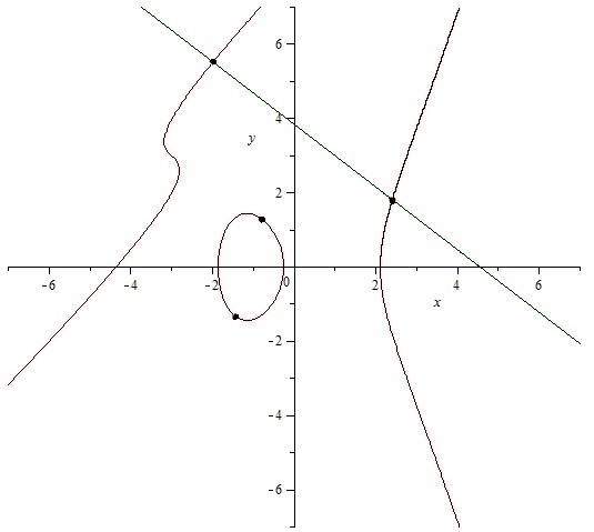
Figure 1: $n=10,k=4,\deg=2$

• For computing ${V_{\bbbr}}=\texttt{LPH}(f)$, we randomly choose a line $l$ in ${\bbbc^{2}}$ and solve $L=\left\{{f,l}\right\}$ by polyhedral homotopy, which follows $D=6$ paths. Then to compute $\Omega$ by linear homotopy, we follow $\left({\begin{array}[]{*{20}{c}}{2-1}\\ {2-1}\end{array}}\right){(6-1)^{2-1}}6=30$ convergent paths, and for ${V_{\bbbr}}$ by linear homotopy, we follow 30 paths, of which 6 are convergent and 19 divergent. Then

  $${V_{\bbbr}}=\left\{{\begin{array}[]{*{20}{c}}{(-1.44299,-1.32941),}&{(-0.781143,1.28371)}\end{array}}\right\}$$

• For computing ${W_{\bbbr}}(f)$, we solve ${f^{(1)}}=\left\{{f,x\cdot\beta+c}\right\}$ by polyhedral homotopy, with $x\cdot\beta+c=0.874645x+1.0351y-3.9825$ and

  $${W_{\bbbr}}({f^{(1)}})=\left\{{\begin{array}[]{*{20}{c}}{(2.4052801,1.815026),}&{(-1.992641,5.531208)}.\end{array}}\right\}$$

  So ${W_{\bbbr}}(f)={W_{\bbbr}}({f^{(1)}})\cup{V_{\bbbr}}$, which has at least one point in each connected component of ${V_{\bbbr}}(f)$ as in Fig. 1.

6 Experiment Performance

As shown in Section 5, to compute the set ${W_{\bbbr}}(f)$, the key and most time consuming steps are solving the system $F=\left\{{f,\sum\limits_{i=1}^{k}{{\lambda_{i}}\nabla{f_{i}}}-\beta}\right\}$ in Algorithm 1. In this section, given $f=\left\{{{f_{1}},\ldots,{f_{k}}}\right\}$, we solve the square system $F=\left\{{f,\sum\limits_{i=1}^{k}{{\lambda_{i}}\nabla{f_{i}}}-\beta}\right\}$. We compare our program LPH which implements Algorithm 1 to Hom4PS-2.0 (available at http://www.math.msu.edu/ li). All the examples were computed on a PC with Intel Core i5 processor (2.5GHz CPU, 4 Cores and 6 GB RAM) in the Windows environment. We mention that LPH is a program written in C++, available at http://arcnl.org/PDF/LHP.zip, and an interface of Maple is provided on this site.

6.1 Dense Examples

Table 1: Dense Examples

$n$	$k$	T1	T2	RAT
2	1	0.125s	0.094s	1.32
3	1	0.125s	0.109s	1.14
3	2	0.125s	0.109s	1.14
4	1	0.125s	0.109s	1.14
4	2	0.156s	0.156s	1.00
4	3	0.202s	0.265s	0.76
5	1	0.125s	0.109s	1.14
5	2	0.187s	0.202s	0.93
5	3	0.390s	0.655s	0.59
5	4	0.687s	1.280s	0.54
6	1	0.140s	0.109s	1.28
6	2	0.281s	0.328s	0.86
6	3	0.76s	1.68s	0.45
6	4	1.61s	4.36s	0.37
6	5	1.90s	6.59s	0.29
7	1	0.14s	0.10s	1.29
7	2	0.344s	0.56s	0.61
7	3	1.3s	3.82s	0.34
7	4	3.7s	14.1s	0.27
7	5	6.318s	27.9s	0.23
7	6	6.006s	27.6s	0.21
8	1	0.15s	0.15s	1.00
8	2	0.54s	0.73s	0.74
8	3	2.29s	7.2s	0.31
8	4	8.018s	34.1s	0.23
8	5	17.6s	91.2s	0.19
8	6	23.7s	153s	0.15
8	7	19.4s	128s	0.15
9	1	0.2s	0.18s	1.08
9	2	0.7s	1.2s	0.58
9	3	4.1s	13.1s	0.31
9	4	16.1s	1m19s	0.20
9	5	46.5s	4m29s	0.17
9	6	1m20s	9m38s	0.138
9	7	1m30s	11m10s	0.135
9	8	59.9s	7m52s	0.126
10	1	0.23s	0.18s	1.25
10	2	0.98s	1.9s	0.51
10	3	5.8s	24.8s	0.24
10	4	31.1s	2m53s	0.18
10	5	1m46s	11m30s	0.15
10	6	3m41s	29m15s	0.13
10	7	5m10s	48m32s	0.107
10	8	4m57s	48m27s	0.102
10	9	3m2s	30m7.553s	0.1

$n$	$k$	T1	T2	RAT
11	1	0.28s	0.23s	1.37
11	2	1.20s	2.85s	0.42
11	3	8.7s	41.5s	0.209
11	4	51.5s	5m25s	0.158
11	5	3m15s	25m30s	0.128
11	6	9m1s	76m32s	0.118
11	7	16m14s	2h.45m30s	0.098
11	8	18m34s	3h52m52s	0.079
11	9	16m22s	3h34m38s	0.076
11	10	6m37s	overflow	$\varepsilon$
12	1	0.29s	0.218s	1.360
12	2	1.27s	4.3s	0.294
12	3	13.5s	1m10s	0.191
12	4	1m25s	10m0.2s	0.142
12	5	6m17s	53m58s	0.116
12	6	20m1s	3h15m10s	0.102
12	7	44m23s	8h7m1s	0.091
12	8	1h8m30s	14h38m24s	0.0779
12	9	1h8m42s	overflow	$\varepsilon$
12	10	46m21s	overflow	$\varepsilon$
12	11	21m54s	overflow	$\varepsilon$
13	1	0.343s	0.218s	1.573
13	2	1.716s	6.193s	0.277
13	3	18s	1m51s	0.61
13	4	2m15s	18m35s	0.121
13	5	11m10s	1h52m27s	0.099
13	6	40m6s	7h16m34s	0.092
13	7	1h39m40s	21h25m14s	0.078
13	8	2h58m48s	overflow	$\varepsilon$
13	9	3h59m32s	overflow	$\varepsilon$
13	10	3h40m3s	overflow	$\varepsilon$
13	11	2h13m9s	overflow	$\varepsilon$
13	12	56m48.309s	overflow	$\varepsilon$
14	2	2.5s	9.6s	0.264
14	3	24.3s	3m0.4s	0.134
14	4	3m19s	37m19s	0.089
14	5	19m28s	8h24m29s	0.038
14	6	1h16m20s	15h58m59s	0.079
14	7	3h34m52s	overflow	$\varepsilon$
14	8	7h50m34s	overflow	$\varepsilon$
14	9	12h43m8s	overflow	$\varepsilon$
14	10	16h48m4s	overflow	$\varepsilon$
14	11	13h9m8s	overflow	$\varepsilon$
14	12	6h29m37s	overflow	$\varepsilon$
14	13	2h18m27s	overflow	$\varepsilon$

In Table 1, we provide the timings of LPH and Hom4ps-2.0 for solving systems $F=\left\{{f,\sum\limits_{i=1}^{k}{{\lambda_{i}}\nabla{f_{i}}}-\beta}\right\}$, where $f=({f_{1}},\ldots,{f_{k}})$ consists of dense polynomials of degree 2, $n=2,...,14$ and $1\leqslant k\leqslant n-1$. T1 ,T2 are the the timings for LPH and Hom4ps-2.0, respectively, and RAT is the ratio of T1 to T2. ‘overflow’ means running out of memory. When T2=overflow, we set RAT=$\varepsilon$.

It may be observed that LPH is much faster than Hom4ps-2.0 when $k>1$. Note also that LPH is a little bit slower than Hom4ps-2.0 when $k=1$. The main reason is obvious. That is, the root number bound of LPH, i.e. $\left({\begin{array}[]{*{20}{c}}{n-1}\\ {n-k}\end{array}}\right){(d-1)^{n-k}}D,$ is close to the mixed volume $MV(F)$ when $F$ is dense but the computation of $MV(F)$ is very time-consuming.

6.2 Sparse Examples

Table 2: Sparse Examples

Ex	$n$	$k$	$d$	term	#1	#2	#	T1	T2	RAT
C2	5	4	4-5	7-32	2*1767	692	383	16.6s	19.4s	0.85
M3	9	5	2	2-7	2*2240	368	32	69s	6s	11
G2	5	2	4	8-9	2*1080	17	15	8.4s	0.2s	31.8
H1	8	6	1-3	2-4	2*400	15	15	9.8s	0.18s	52
H2	8	5	2-4	3-5	2*12320	148	80	5m49s	1.2s	267

In Table 2, we provide the timings of LPH and Hom4ps-2.0 on sparse examples: Czapor Geddes2, Morgenstern AS(3or), Gerdt2, Hairer1, and Hawes2 which are available at : http://www-sop.inria.fr/saga/POL/. #1 and #2 is the number of curves followed by LPH and Hom4ps-2.0, respectively. # is the number of roots of the Jacobian systems constructed from the examples. ‘$d$’ means the minimal and maximal degree of the example. “term” means the minimal and maximal number of terms of the example. T1 and T2 are the timings of LPH and Hom4ps-2.0, respectively. RAT means the ratio of T1 to T2.

Note that LPH is much slower than Hom4ps on these sparse examples. The main reason is that LPH pays the overhead cost for the $\Omega$ and homotopy

$${H_{2}}(x,\lambda,t)=G\cdot(1-t)+F\cdot{\gamma_{2}}\cdot t.$$

Moreover, LPH executes $2*\left({\begin{array}[]{*{20}{c}}{n-1}\\ {k-1}\end{array}}\right){(d-1)^{n-k}}D$ times of curve following, while Hom4ps does only $MV(F)$ times of curve following. $\left({\begin{array}[]{*{20}{c}}{n-1}\\ {k-1}\end{array}}\right){(d-1)^{n-k}}D$ is not tight for these sparse examples and much greater than $MV(F)$.

6.3 RAT/Density

Figure 2: RAT and Density

In Fig. 2, we present the changes of ratio of T1 to T2 as terms increase. We randomly generate $f=({f_{1}},\ldots,{f_{k}})$ with different $n,k$ and degrees, and increase the number of terms from 2 to dense.

It can be observed that, when the polynomials are not very sparse, e.g. the number of terms are more than $10\%$ of $\left({\begin{array}[]{*{20}{c}}{n+d}\\ {d}\end{array}}\right)$, LPH is faster than Hom4ps-2.0. Actually, when the polynomials are not very sparse, the root number bound $\left({\begin{array}[]{*{20}{c}}{n-1}\\ {k-1}\end{array}}\right){(d-1)^{n-k}}D$ is close to $MV(F)$.

7 Acknowledgement

We gratefully acknowledge the very helpful suggestions of Hoon Hong on this paper with emphasize on Section 6. We also thank Changbo Chen for his helpful comments.

References

- [1] Garcia, C.B., Zangwill, W.I.: Finding all solutions to polynomial systems and other systems of equations. Mathematical Programming 16(1) (1979) 159–176
- [2] Drexler, F.J.: Eine methode zur berechnung sämtlicher lösungen von polynomgleichungssystemen. Numerische Mathematik 29(1) (1977) 45–58
- [3] Sommese, A.J., Verschelde, J., Wampler, C.W.: Numerical algebraic geometry. In: The Mathematics of Numerical Analysis, volume 32 of Lectures in Applied Mathematics, AMS (1996) 749–763
- [4] Allgower, E.L., Georg, K.: Introduction to numerical continuation methods. Reprint of the 1979 original. Society for Industrial and Applied Mathematics (2003)
- [5] Li, T.: Numerical solution of polynomial systems by homotopy continuation methods. In: Handbook of Numerical Analysis. Volume 11 of Handbook of Numerical Analysis. Elsevier (2003) 209 – 304
- [6] Sommese, A.J., Wampler, C.W.: The numerical solution of systems of polynomials arising in engineering and science /. World Scientific, (2005)
- [7] Morgan, A.: Solving Polynominal Systems Using Continuation for Engineering and Scientific Problems. Society for Industrial and Applied Mathematics, Philadelphia, PA, USA (2009)
- [8] Bates, D.J., Haunstein, J.D., Sommese, A.J., Wampler, C.W.: Numerically Solving Polynomial Systems with Bertini. Society for Industrial and Applied Mathematics, Philadelphia, PA, USA (2013)
- [9] Lee, T.L., Li, T.Y., Tsai, C.H.: Hom4ps-2.0: a software package for solving polynomial systems by the polyhedral homotopy continuation method. Computing 83(2) (2008) 109
- [10] Morgan, A.P., Sommese, A.J., Watson, L.T.: Finding all isolated solutions to polynomial systems using hompack. ACM Trans. Math. Softw. 15(2) (June 1989) 93–122
- [11] Verschelde, J.: Algorithm 795: Phcpack: A general-purpose solver for polynomial systems by homotopy continuation. ACM Trans. Math. Softw. 25(2) (June 1999) 251–276
- [12] Collins, G.: Quantifier elimination for real closed fields by cylindrical algebraic decompostion. In: Automata Theory and Formal Languages 2nd GI Conference Kaiserslautern, May 20–23, 1975. Volume 33 of LNCS. Springer (1975) 134–183
- [13] Seidenberg, A.: A new decision method for elementary algebra. Annals of Mathematics 60(2) (1954) 365–374
- [14] Rouillier, F., Roy, M.F., Safey El Din, M.: Finding at least one point in each connected component of a real algebraic set defined by a single equation. Journal of Complexity 16(4) (2000) 716 – 750
- [15] Safey El Din, M., Schost, E.: Polar varieties and computation of one point in each connected component of a smooth real algebraic set. In: Proceedings of the 2003 International Symposium on Symbolic and Algebraic Computation. ISSAC ’03, New York, NY, USA, ACM (2003) 224–231
- [16] Safey El Din, M., Spaenlehauer, P.J.: Critical point computations on smooth varieties: Degree and complexity bounds. In: Proceedings of the ACM on International Symposium on Symbolic and Algebraic Computation. ISSAC ’16, New York, NY, USA, ACM (2016) 183–190
- [17] Bank, B., Giusti, M., Heintz, J., Pardo, L.M.: Generalized polar varieties and an efficient real elimination. Kybernetika 40(5) (2004) [519]–550
- [18] Bank, B., Giusti, M., Heintz, J., Pardo, L.: Generalized polar varieties: geometry and algorithms. Journal of Complexity 21(4) (2005) 377 – 412
- [19] Li, T.Y., Wang, X.: Solving real polynomial systems with real homotopies. Mathematics of Computation 60(202) (1993) 669–680
- [20] Lu, Y., Bates, D.J., Sommese, A.J., Wampler, C.W.: Finding all real points of a complex curve. Technical report, In Algebra, Geometry and Their Interactions (2006)
- [21] Bates, D.J., Sottile, F.: Khovanskii-rolle continuation for real solutions. Found. Comput. Math. 11(5) (October 2011) 563–587
- [22] Besana, G.M., Rocco, S., Hauenstein, J.D., Sommese, A.J., Wampler, C.W.: Cell decomposition of almost smooth real algebraic surfaces. Numer. Algorithms 63(4) (August 2013) 645–678
- [23] Hauenstein, J.D.: Numerically computing real points on algebraic sets. Acta Applicandae Mathematicae 125(1) (2013) 105–119
- [24] Shen, F., Wu, W., Xia, B.: Real Root Isolation of Polynomial Equations Based on Hybrid Computation. In: Computer Mathematics: 9th Asian Symposium (ASCM2009). Springer Berlin Heidelberg (2014) 375–396
- [25] Wu, W., Reid, G.: Finding points on real solution components and applications to differential polynomial systems. In: Proceedings of the 38th International Symposium on Symbolic and Algebraic Computation. ISSAC ’13, New York, NY, USA, ACM (2013) 339–346
- [26] Wu, W., Reid, G., Feng, Y.: Computing real witness points of positive dimensional polynomial systems. Theoretical Computer Science (2017) – Available online March 31, 2017. http://doi.org/10.1016/j.tcs.2017.03.035.
- [27] Bernshtein, D.N.: The number of roots of a system of equations. Functional Analysis and Its Applications 9(3) (1975) 183–185
- [28] Hauenstein, J.D., Sommese, A.J., Wampler, C.W.: Regeneration homotopies for solving systems of polynomials. Math. Comp. 80(273) (2011) 345–377
- [29] John, F.: Extremum Problems with Inequalities as Subsidiary Conditions. Springer Basel (2014)
- [30] Morgan, A.P., Sommese, A.J.: Coefficient-parameter polynomial continuation. Applied Mathematics and Computation 29(2) (1989) 123 – 160
- [31] Morgan, A.P., Sommese, A.J., Wampler, C.W.: A power series method for computing singular solutions to nonlinear analytic systems. Numerische Mathematik 63(1) (1992) 391–409
- [32] Morgan, A.P.: A transformation to avoid solutions at infinity for polynomial systems. Applied Mathematics and Computation 18(1) (1986) 77 – 86
- [33] Huber, B., Verschelde, J.: Polyhedral end games for polynomial continuation. Numerical Algorithms 18(1) (1998) 91–108
- [34] Bates, D.J., Hauenstein, J.D., Sommese, A.J. In: A parallel endgame. Providence, RI: American Mathematical Society (AMS) (2011) 25–35