Sufficient Markov Decision Processes with Alternating Deep Neural Networks

Abstract

Advances in mobile computing technologies have made it possible to monitor and apply data-driven interventions across complex systems in real time. Recent and high-profile examples of data-driven decision making include autonomous vehicles, intelligent power grids, and precision medicine through mobile health. Markov decision processes are the primary mathematical model for sequential decision problems with a large or indefinite time horizon; existing methods for estimation and inference rely critically on the correctness of this model. Mathematically, this choice of model incurs little loss in generality as any decision process evolving in discrete time with observable process states, decisions, and outcomes can be represented as a Markov decision process. However, in some application domains, e.g., mobile health, choosing a representation of the underlying decision process that is both Markov and low-dimensional is non-trivial; current practice is to select a representation using domain expertise. We propose an automated method for constructing a low-dimensional representation of the original decision process for which: (P1) the Markov decision process model holds; and (P2) a decision strategy that leads to maximal mean utility when applied to the low-dimensional representation also leads to maximal mean utility when applied to population of interest. Our approach uses a novel deep neural network to define a class of potential process representations and then searches within this class for the representation of lowest dimension which satisfies (P1) and (P2). We illustrate the proposed method using a suite of simulation experiments and application to data from a mobile health intervention targeting smoking and heavy episodic drinking among college students.

1 Introduction

Sequential decision problems arise in a wide range of application domains including autonomous vehicles (Bagnell and Schneider, 2001), finance (Bäuerle and Rieder, 2011), logistics (Zhang and Dietterich, 1995), robotics (Kober et al., 2013), power grids (Riedmiller et al., 2000), and healthcare (Chakraborty and Moodie, 2013). Markov decision processes (MDPs) (Bellman, 1957; Puterman, 2014) are the primary mathematical model for representing sequential decision problems with an indefinite time horizon (Bertsekas and Tsitsiklis, 1996; Sutton and Barto, 1998; Bather, 2000; Si, 2004; Powell, 2007; Wiering and Van Otterlo, 2012). This class of models is quite general as almost any decision process can be made into an MDP by concatenating data over multiple decision points (see Section 2 for a precise statement); however, coercing a decision process into the MDP framework in this way can lead to high-dimensional system state information that is difficult to model effectively. One common approach to construct a low-dimensional decision process from a high-dimensional MDP is to create a finite discretization of the space of possible system states and to treat the resultant process as a finite MDP (Gordon, 1995; Murao and Kitamura, 1997; Sutton and Barto, 1998; Kamio et al., 2004; Whiteson et al., 2007). However, such discretization can result in a significant loss of information and can be difficult to apply when the system state information is continuous and high-dimensional. Another common approach to dimension reduction is to construct a low-dimensional summary of the underlying system states, e.g., by applying principal components analysis (Jolliffe, 1986), multidimensional scaling (Borg and Groenen, 1997), or by constructing a local linear embedding (Roweis and Saul, 2000). These approaches can identify a low-dimensional representation of the system state but, as we shall demonstrate, they need not retain salient features for making good decisions.

The preceding methods seek to construct a low-dimensional representation of a high-dimensional MDP with the goal of using the low-dimensional representation to estimate an optimal decision strategy, i.e., one that leads to maximal mean utility when applied to the original process; however, they offer no guarantee that the resulting process is an MDP or that a decision strategy estimated using data from the low-dimensional process will perform well when applied to the original process. We derive sufficient conditions under which a low-dimensional representation is an MDP, and that an optimal decision strategy for this low-dimensional representation is optimal for the original process. We develop a hypothesis test for this sufficient condition based on the Brownian distance covariance (Székely et al., 2007; Székely and Rizzo, 2009) and use this test as the basis for selecting a low-dimensional representation within a class of deep neural networks. The proposed estimator can be viewed as a novel variant of deep neural networks for feature construction in MDPs.

In Section 2, we review the MDP model for sequential decision making and define an optimal decision strategy. In Section 3, we derive conditions under which a low-dimensional representation of an MDP is sufficient for estimating an optimal decision strategy for the original process. In Section 4, we develop a new deep learning algorithm that is designed to produce low-dimensional representation that satisfies the proposed sufficiency condition. In Section 5, we evaluate the performance of the proposed method in a suite of simulated experiments. In Section 6, we illustrate the proposed method using data from a study of a mobile health intervention targeting smoking and heavy episodic drinking among college students (Witkiewitz et al., 2014). A discussion of future work is given in Section 7.

2 Setup and Notation

We assume that the observed data are $\left\{\left(\mathbf{S}_{i}^{1},A_{i}^{1},U_{i}^{1},\mathbf{S}_{i}^{2},\ldots,A_{i}^{T},U_{i}^{T},\mathbf{S}_{i}^{T+1}\right)\right\}_{i=1}^{n}$ which comprise $n$ independent and identically distributed copies of the trajectory $(\mathbf{S}^{1},A^{1},U^{1},\mathbf{S}^{2},\ldots,\allowbreak A^{T},U^{T},\mathbf{S}^{T+1})$ where: $T\in\mathbb{N}$ denotes the observation time; $\mathbf{S}^{t}\in\mathbb{R}^{p_{t}}$ denotes a summary of information collected up to time $t=1,\ldots,T$; $A^{t}\in\mathcal{A}=\left\{1,\ldots,K\right\}$ denotes the decision made at time $t=1,\ldots,T$; and $U^{t}=U^{t}(\mathbf{S}^{t},A^{t},\mathbf{S}^{t+1})$ is a real-valued deterministic function of $(\mathbf{S}^{t},A^{t},\mathbf{S}^{t+1})$ that quantifies the momentary “goodness” of being in state $\mathbf{S}^{t}$, making decision $A^{t}$, and subsequently transitioning to state $\mathbf{S}^{t+1}$. We assume throughout that $\sup_{t}|U^{t}|\leq M$ with probability one for some fixed constant $M$. In applications like mobile health, the observed data might be collected in a pilot study with a preset time horizon $T$ (Maahs et al., 2012; Witkiewitz et al., 2014); however, the intent is to use these data to estimate an intervention strategy that will maximize some measure of cumulative utility when applied over an indefinite time horizon (Ertefaie, 2014; Liao et al., 2015; Luckett et al., 2016). Thus, we assume that $(\mathbf{S}^{1},A^{1},U^{1},\mathbf{S}^{2},\ldots,A^{T},U^{T},\mathbf{S}^{T+1})$ comprises the first $T$ observations of the process $(\mathbf{S}^{1},A^{1},U^{1},\mathbf{S}^{2},\ldots)$. Furthermore, we assume (A0) that this infinite process is Markov and homogeneous in that it satisfies

$$P\left(\mathbf{S}^{t+1}\in\mathcal{G}^{t+1}\bigg{|}A^{t},\mathbf{S}^{t},\ldots,A^{1},\mathbf{S}^{1}\right)=P\left(\mathbf{S}^{t+1}\in\mathcal{G}^{t+1}\bigg{|}A^{t},\mathbf{S}^{t}\right),$$ (1)

for all (measurable) subsets $\mathcal{G}^{t+1}\subseteq\mathrm{dom}\,\mathbf{S}^{t+1}$ and $t\in\mathbb{N}$ and that the probability measure in (1) does not depend on $t$. For any process $(\mathbf{S}^{1},A^{1},\mathbf{S}^{2},\ldots)$ one can define $\widetilde{\mathbf{S}}^{t}=(\mathbf{S}^{t},A^{t-1},\ldots,\mathbf{S}^{t-m_{t}})$, where $m_{t}$ is chosen so that process $\left(\widetilde{\mathbf{S}}^{1},A^{t},\widetilde{\mathbf{S}}^{t},\ldots\right)$ satisfies (A0); to see this, note that the result holds trivially for $m_{t}=t-1$. Furthermore, by augmenting the state with a variable for time, i.e., defining the new state at time $t$ to be $(\widetilde{S}^{t},t)$, one can ensure that the probability measure in (A0) does not depend on $t$. In practice, $m_{t}$ is typically chosen to be a constant, as letting the dimension of the state grow with time makes extrapolation beyond the observed time horizon, $T$, difficult. Thus, hereafter we assume that the domain of the state is constant over time, i.e., $\mathrm{dom}\,\mathbf{S}^{t}=\mathcal{S}\subseteq\mathbb{R}^{p}$ for all $t\in\mathbb{N}$. Furthermore, we assume that the utility is homogeneous in time, i.e., $U^{t}=U(\mathbf{S}^{t},A^{t},\mathbf{S}^{t+1})$ for all $t\in\mathbb{N}$.

A decision strategy, $\pi:\mathcal{S}\rightarrow\mathcal{A}$, is a map from states to decisions so that, under $\pi$, a decision maker presented with $\mathbf{S}^{t}=\mathbf{s}^{t}$ at time $t$ will select decision $\pi(\mathbf{s}^{t})$. We define an optimal decision strategy using the language of potential outcomes (Rubin, 1978). We use an overline to denote history so that $\overline{\mathbf{a}}^{t}=(a^{1},\ldots,a^{t})$ and $\overline{\mbox{\bf s}}^{t}=(\mbox{\bf s}^{1},\ldots,\mbox{\bf s}^{t})$. The set of potential outcomes is $\mathbf{O}^{*}=\left\{\mathbf{S}^{*t}(\overline{\mathbf{a}}^{t-1})\right\}_{t\geq 1}$ where $\mathbf{S}^{*t}(\overline{\mathbf{a}}^{t-1})$ is the potential state under $\overline{\mathbf{a}}^{t-1}$ and we have defined $\mathbf{S}^{*1}(\overline{\mathbf{a}}^{0})=\mathbf{S}^{1}$. Thus, the potential utility at time $t$ under $\overline{\mathbf{a}}^{t}$ is $U\left\{\mathbf{S}^{*t}(\overline{\mathbf{a}}^{t-1}),a^{t},\mathbf{S}^{*(t+1)}(\overline{\mathbf{a}}^{t})\right\}$. The potential state under a decision strategy, $\pi$, is $\mathbf{S}^{*t}(\pi)=\sum_{\overline{\mathbf{a}}^{t-1}}\mathbf{S}^{*t}(\overline{\mathbf{a}}^{t-1})\prod_{v=1}^{t-1}1_{\pi\{\mathbf{S}^{*v}(\overline{\mathbf{a}}^{v-1})\}=a^{v}}$, and the potential utility under $\pi$ is $U^{*t}(\pi)=U\left[\mathbf{S}^{*t}(\pi),\pi\left\{\mathbf{S}^{*t}(\pi)\right\},\mathbf{S}^{*(t+1)}(\pi)\right]$. Define the discounted mean utility under a decision strategy, $\pi$, as

$$V(\pi)=\mathbb{E}\left\{\sum_{t\geq 1}\gamma^{t-1}U^{*t}(\pi)\right\},$$

where $\gamma\in(0,1)$ is a discount factor that balances the trade-off between immediate and long-term utility. Given a class of decision strategies, $\Pi$, an optimal decision strategy, $\pi^{\mathrm{opt}}\in\Pi$, satisfies $V(\pi^{\mathrm{opt}})\geq V(\pi)$ for all $\pi\in\Pi$.

Define $\mu^{t}(\mathbf{a}^{t};\overline{\mbox{\bf s}}^{t},\overline{\mathbf{a}}^{t-1})=P\left(A^{t}=a^{t}\big{|}\overline{\mathbf{S}}^{t}=\overline{\mbox{\bf s}}^{t},\overline{\mbox{\bf A}}^{t-1}=\overline{\mathbf{a}}^{t-1}\right)$. To characterize $\pi^{\mathrm{opt}}$ in terms of the data-generating model, we make the following assumptions for all $t\in\mathbb{N}$: (C1) consistency, $\mathbf{S}^{t}=\mathbf{S}^{*t}(\overline{\mbox{\bf A}}^{t-1})$; (C2) positivity, there exists $\epsilon>0$ such that $\mu^{t}(\mathbf{a}^{t};\overline{\mathbf{S}}^{t},\overline{\mbox{\bf A}}^{t-1})\geq\epsilon$ with probability one for all $a^{t}\in\mathcal{A}$; and (C3) sequential ignorability, $\mathbf{O}^{*}\perp A^{t}\big{|}\overline{\mathbf{S}}^{t},\overline{\mbox{\bf A}}^{t-1}$. These assumptions are standard in data-driven decision making (Robins, 2004; Schulte et al., 2014). Assumptions (C2) and (C3) hold by design in a randomized trial (Liao et al., 2015; Klasnja et al., 2015) but are not verifiable in the data for observational studies. Under these assumptions, the joint distribution of $\left\{\mathbf{S}^{*t}(\pi)\right\}_{t=1}^{T}$ is non-parametrically identifiable under the data-generating model for any decision strategy $\pi$ and time horizon $T$. In our application, these assumptions will enable us to construct low-dimensional features of the state that retain all relevant information for estimating $\pi^{\mathrm{opt}}$ without having to solve the original MDP as an intermediate step.

3 Sufficient Markov Decision Processes

If the states $\mathbf{S}^{t}$ are high-dimensional it can be difficult to construct a high-quality estimator of the optimal decision strategy; furthermore, in applications like mobile health, storage and computational resources on the mobile device are limited, making it desirable to store only as much information as is needed to inform decision making. For any map $\phi:\mathcal{S}\rightarrow\mathbb{R}^{q}$ define $\mathbf{S}_{\phi}^{t}=\phi(\mathbf{S}^{t})$. We say that $\phi$ induces a sufficient MDP for $\pi^{\mathrm{opt}}$ if $(\overline{\mbox{\bf A}}^{t},\overline{\mathbf{S}}_{\phi}^{t+1},\overline{\mbox{\bf U}}^{t})$ contains all relevant information in $(\overline{\mbox{\bf A}}^{t},\overline{\mathbf{S}}^{t+1},\overline{\mbox{\bf U}}^{t})$ about $\pi^{\mathrm{opt}}$. Given a policy $\pi_{\phi}:\mathrm{dom}\,\mathbf{S}_{\phi}^{t}\rightarrow\mathcal{A}$ define the potential utility under $\pi_{\phi}$ as

$$U_{\phi}^{*t}(\pi_{\phi})=\sum_{\overline{\mathbf{a}}^{t}}U\left\{\mathbf{S}^{*t}\left(\overline{\mathbf{a}}^{t-1}\right),a^{t},\mathbf{S}^{*(t+1)}\left(\overline{\mathbf{a}}^{t}\right)\right\}\prod_{v=1}^{t}1_{\pi_{\phi}\left\{\mathbf{S}_{\phi}^{*v}(\overline{\mathbf{a}}^{v-1})\right\}=a^{v}}.$$

The following definition formalizes the notion of inducing a sufficient MDP.

Definition 3.1.

Let $\Pi\subseteq\mathcal{A}^{\mathcal{S}}$ denote a class of decision strategies defined on $\mathcal{S}$ and $\Pi_{\phi}\subseteq\mathcal{A}^{\mathcal{S}_{\phi}}$ a class of decision strategies defined on $\mathcal{S}_{\phi}=\mathrm{dom}\,\mathbf{S}_{\phi}^{t}\subseteq\mathbb{R}^{q}$. We say that the pair $(\phi,\Pi_{\phi})$ induces a sufficient MDP for $\pi^{\mathrm{opt}}$ within $\Pi$ if the following conditions hold for all $t\in\mathbb{N}$:

• the process $(\overline{\mbox{\bf A}}^{t},\overline{\mathbf{S}}_{\phi}^{t+1},\overline{\mbox{\bf U}}^{t})$ is Markov and homogeneous, i.e.,

  $$P\left(\mathbf{S}_{\phi}^{t+1}\in\mathcal{G}_{\phi}^{t+1}\big{|}\overline{\mathbf{S}}_{\phi}^{t},\overline{\mbox{\bf A}}^{t}\right)=P\left(\mathbf{S}_{\phi}^{t+1}\in\mathcal{G}_{\phi}^{t+1}\big{|}{\mathbf{S}}_{\phi}^{t},{A}^{t}\right)$$

  for any (measurable) subset $\mathcal{G}_{\phi}^{t+1}\subseteq\mathbb{R}^{q}$ and this probability does not depend on $t$;

• there exists $\pi^{\mathrm{opt}}\in\arg\max_{\pi\in\Pi}V(\pi)$ which can be written as $\pi^{\mathrm{opt}}=\pi_{\phi}^{\mathrm{opt}}\circ\phi$, where $\pi_{\phi}^{\mathrm{opt}}\in\arg\max_{\pi_{\phi}\in\Pi_{\phi}}\mathbb{E}\left\{\sum_{t\geq 1}\gamma^{t-1}U_{\phi}^{*t}(\pi_{\phi})\right\}$.

Thus, given observed data, $\left\{(\overline{\mathbf{S}}_{i}^{T+1},\overline{\mbox{\bf A}}_{i}^{T},\overline{\mbox{\bf U}}_{i}^{T})\right\}_{i=1}^{n}$ and class of decision strategies, $\Pi$, if one can find a pair $(\phi,\Pi_{\phi})$ which induces a sufficient MDP for $\pi^{\mathrm{opt}}$ within $\Pi$, then it suffices to store only the reduced process $\left\{\left(\overline{\mathbf{S}}_{\phi,i}^{T+1},\overline{\mbox{\bf A}}_{i}^{T},\overline{\mbox{\bf U}}_{i}^{T}\right)\right\}_{i=1}^{n}$. Furthermore, existing reinforcement learning algorithms (e.g., Sutton and Barto, 1998; Szepesvári, 2010) can be applied to this reduced process to construct an estimator of $\pi_{\phi}^{\mathrm{opt}}$ and hence $\pi^{\mathrm{opt}}=\pi_{\phi}^{\mathrm{opt}}\circ\phi$. If the dimension of $\mathbf{S}_{\phi}^{t}$ is substantially smaller than that of $\mathbf{S}^{t}$, then using the reduced process can lead to smaller estimation error as well as reduced storage and computational costs. In some applications, it may also be desirable to have $\phi$ be a sparse function of $\mathbf{S}^{t}$ in the sense that it only depends on a subset of the components of $\mathbf{S}^{t}$. For example, in the context of mobile health, one may construct the state, $\mathbf{S}^{t}$, by concatenating measurements taken at time points $t,t-1,\ldots,t-m$, where the look-back period, $m$, is chosen conservatively based on clinical judgement to ensure that the process is Markov; however, a data-driven sparse feature map might identify that a look-back period of $m^{\prime}\ll m$ is sufficient thereby reducing computational and memory requirements but also generating new knowledge that may be of clinical value. The remainder of this section will focus on developing verifiable conditions for checking that $(\phi,\Pi_{\phi})$ induces a sufficient MDP. These conditions are used to build a data-driven, low-dimensional, and potentially sparse sufficient MDP.

Define $\mbox{\bf Y}^{t+1}=\left\{U^{t},(\mathbf{S}^{t+1})^{\intercal}\right\}^{\intercal}$ for all $t\in\mathbb{N}$. The following result provides a conditional independence criterion that ensures a given feature map induces a sufficient MDP; this criterion can be seen as an MDP analog of nonlinear sufficient dimension reduction in regression (Cook, 2007; Li et al., 2011). A proof is provided in the Supplemental Materials.

Theorem 3.2.

Let $(\mathbf{S}^{1},A^{1},U^{1},\mathbf{S}^{2},\ldots)$ be an MDP that satisfies (A0) and (C1)-(C3). Suppose that there exists $\phi:\mathcal{S}\rightarrow\mathbb{R}^{q}$ such that

$$\mbox{\bf Y}^{t+1}\mathchoice{\mathrel{\hbox to0.0pt{$\displaystyle\perp$\hss}\mkern 2.0mu{\displaystyle\perp}}}{\mathrel{\hbox to0.0pt{$\textstyle\perp$\hss}\mkern 2.0mu{\textstyle\perp}}}{\mathrel{\hbox to0.0pt{$\scriptstyle\perp$\hss}\mkern 2.0mu{\scriptstyle\perp}}}{\mathrel{\hbox to0.0pt{$\scriptscriptstyle\perp$\hss}\mkern 2.0mu{\scriptscriptstyle\perp}}}\mathbf{S}^{t}\big{|}\mathbf{S}_{\phi}^{t},A^{t},$$ (2)

then, $(\phi,\Pi_{\phi,\mathrm{msbl}})$ induces a sufficient MDP for $\pi^{\mathrm{opt}}$ within $\Pi_{\mathrm{msbl}}$, where $\Pi_{\mathrm{msbl}}$ is the set of measurable maps from $\mathcal{S}$ into $\mathcal{A}$ and $\Pi_{\phi,\mathrm{msbl}}$ is the set of measurable maps from $\mathbb{R}^{q}$ into $\mathcal{A}$.

The preceding result could be used to construct an estimator for $\phi$ so that $(\phi,\Pi_{\phi,\mathrm{msbl}})$ induces a sufficient MDP for $\pi^{\mathrm{opt}}$ within $\Pi_{\mathrm{msbl}}$ as follows. Let $\Phi$ denote a potential class of vector-valued functions on $\mathcal{S}$. Let $\widehat{p}_{n}(\phi)$ denote a p-value for a test of the conditional independence criterion (2) based on the mapping $\phi$, e.g., one might construct this p-value using conditional Brownian distance correlation (Wang et al., 2015) or kernel-based tests of conditional independence (Fukumizu et al., 2007). Then, one could select $\widehat{\phi}_{n}$ to be the transformation of lowest dimension among those within the set $\left\{\phi\in\Phi\,:\,\widehat{d}_{n}(\phi)\geq\tau\right\}$, where $\tau$ is a fixed significance level, e.g., $\tau=0.10$. However, such an approach can be computationally burdensome especially if the class $\Phi$ is large. Instead, we will develop a procedure based on a series of unconditional tests that is computationally simpler and allows for a flexible class of potential transformations. Before presenting this approach, we first describe how the conditional independence criterion in the above theorem can be applied recursively to potentially produce a sufficient MDP of lower dimension.

The condition $\mbox{\bf Y}^{t+1}\mathchoice{\mathrel{\hbox to0.0pt{$\displaystyle\perp$\hss}\mkern 2.0mu{\displaystyle\perp}}}{\mathrel{\hbox to0.0pt{$\textstyle\perp$\hss}\mkern 2.0mu{\textstyle\perp}}}{\mathrel{\hbox to0.0pt{$\scriptstyle\perp$\hss}\mkern 2.0mu{\scriptstyle\perp}}}{\mathrel{\hbox to0.0pt{$\scriptscriptstyle\perp$\hss}\mkern 2.0mu{\scriptscriptstyle\perp}}}\mathbf{S}^{t}\big{|}\mathbf{S}_{\phi}^{t},A^{t}$ is overly stringent in that it requires $\mathbf{S}_{\phi}^{t}$ to capture all the information about $\mbox{\bf Y}^{t+1}$ contained within $\mathbf{S}^{t}$ regardless of whether or not that information is useful for decision making. However, given a sufficient MDP $(\mathbf{S}_{\phi}^{1},A^{1},U^{1},\mathbf{S}_{\phi}^{2},\ldots)$, one can apply the above theorem to this MDP to obtain further dimension reduction; this process can be iterated until no further dimension reduction is possible. For any map $\phi:\mathcal{S}\rightarrow\mathbb{R}^{q}$, define $\mbox{\bf Y}_{\phi}^{t}=\left\{U^{t},\left(\mathbf{S}_{\phi}^{t+1}\right)^{\intercal}\right\}^{\intercal}$. The following result is proved in the Supplemental Materials.

Corollary 3.3.

Let $(\mathbf{S}^{1},A^{1},U^{1},\mathbf{S}^{2},\ldots)$ be an MDP that satisfies (A0) and (C1)-(C3). Assume that there exists $\phi_{0}:\mathcal{S}\rightarrow\mathbb{R}^{q_{0}}$ such that $(\phi_{0},\Pi_{\phi_{0},\mathrm{msrbl}})$ induces a sufficient MDP for $\pi^{\mathrm{opt}}$ within $\Pi_{\mathrm{msrbl}}$. Suppose that there exists $\phi_{1}:\mathbb{R}^{q_{0}}\rightarrow\mathbb{R}^{q_{1}}$ such that for all $t\in\mathbb{N}$

$$\mbox{\bf Y}_{\phi_{0}}^{t+1}\mathchoice{\mathrel{\hbox to0.0pt{$\displaystyle\perp$\hss}\mkern 2.0mu{\displaystyle\perp}}}{\mathrel{\hbox to0.0pt{$\textstyle\perp$\hss}\mkern 2.0mu{\textstyle\perp}}}{\mathrel{\hbox to0.0pt{$\scriptstyle\perp$\hss}\mkern 2.0mu{\scriptstyle\perp}}}{\mathrel{\hbox to0.0pt{$\scriptscriptstyle\perp$\hss}\mkern 2.0mu{\scriptscriptstyle\perp}}}\mathbf{S}_{\phi_{0}}^{t}\big{|}\mathbf{S}_{\phi_{1}\circ\phi_{0}}^{t},A^{t},$$ (3)

then $(\phi_{1}\circ\phi_{0},\Pi_{\phi_{1}\circ\phi_{0},\mathrm{msrbl}})$ induces a sufficient MDP for $\pi^{\mathrm{opt}}$ within $\Pi_{\mathrm{msrbl}}$. Furthermore, for $k\geq 2$, denoting $\phi_{k}\circ\phi_{k-1}\circ\cdots\circ\phi_{0}$ as $\overline{\phi}_{k}$, if there exists $\phi_{k}:\mathbb{R}^{q_{k-1}}\rightarrow\mathbb{R}^{q_{k}}$ such that $\mbox{\bf Y}_{\overline{\phi}_{k-1}}^{t+1}\mathchoice{\mathrel{\hbox to0.0pt{$\displaystyle\perp$\hss}\mkern 2.0mu{\displaystyle\perp}}}{\mathrel{\hbox to0.0pt{$\textstyle\perp$\hss}\mkern 2.0mu{\textstyle\perp}}}{\mathrel{\hbox to0.0pt{$\scriptstyle\perp$\hss}\mkern 2.0mu{\scriptstyle\perp}}}{\mathrel{\hbox to0.0pt{$\scriptscriptstyle\perp$\hss}\mkern 2.0mu{\scriptscriptstyle\perp}}}\mathbf{S}_{\overline{\phi}_{k-1}}^{t}\big{|}\mathbf{S}_{\overline{\phi}_{k}}^{t},A^{t}$, then $(\overline{\phi}_{k},\Pi_{\overline{\phi}_{k},\mathrm{msrbl}})$ induces a sufficient MDP for $\pi^{\mathrm{opt}}$ within $\Pi_{\mathrm{msrbl}}$.

We now state a simple condition involving the residuals of a multivariate regression that can be used to test the conditional independence required in each step of the preceding corollary. In our implemenation we use residuals from a varient of deep neural networks that is suited to sequential decision problems (see Section 4). The following result is proved in the Supplemental Materials.

Lemma 3.4.

Let $(\mathbf{S}^{1},A^{1},U^{1},\mathbf{S}^{2},\ldots)$ be an MDP that satisfies (A0) and (C1)-(C3). Suppose that there exists $\phi:\mathcal{S}\rightarrow\mathbb{R}^{q}$ such that at least one of the following conditions hold:

• $\left\{\mbox{\bf Y}^{t+1}-\mathbb{E}\left(\mbox{\bf Y}^{t+1}\big{|}\mathbf{S}_{\phi}^{t},A^{t}\right)\right\}\mathchoice{\mathrel{\hbox to0.0pt{$\displaystyle\perp$\hss}\mkern 2.0mu{\displaystyle\perp}}}{\mathrel{\hbox to0.0pt{$\textstyle\perp$\hss}\mkern 2.0mu{\textstyle\perp}}}{\mathrel{\hbox to0.0pt{$\scriptstyle\perp$\hss}\mkern 2.0mu{\scriptstyle\perp}}}{\mathrel{\hbox to0.0pt{$\scriptscriptstyle\perp$\hss}\mkern 2.0mu{\scriptscriptstyle\perp}}}\mathbf{S}^{t}\big{|}A^{t}$,

• $\left\{\mathbf{S}^{t}-\mathbb{E}\left(\mathbf{S}^{t}\big{|}\mathbf{S}_{\phi}^{t}\right)\right\}\mathchoice{\mathrel{\hbox to0.0pt{$\displaystyle\perp$\hss}\mkern 2.0mu{\displaystyle\perp}}}{\mathrel{\hbox to0.0pt{$\textstyle\perp$\hss}\mkern 2.0mu{\textstyle\perp}}}{\mathrel{\hbox to0.0pt{$\scriptstyle\perp$\hss}\mkern 2.0mu{\scriptstyle\perp}}}{\mathrel{\hbox to0.0pt{$\scriptscriptstyle\perp$\hss}\mkern 2.0mu{\scriptscriptstyle\perp}}}\left(\mbox{\bf Y}^{t+1},\mathbf{S}_{\phi}^{t}\right)\big{|}A^{t},$

then $\mbox{\bf Y}^{t+1}\mathchoice{\mathrel{\hbox to0.0pt{$\displaystyle\perp$\hss}\mkern 2.0mu{\displaystyle\perp}}}{\mathrel{\hbox to0.0pt{$\textstyle\perp$\hss}\mkern 2.0mu{\textstyle\perp}}}{\mathrel{\hbox to0.0pt{$\scriptstyle\perp$\hss}\mkern 2.0mu{\scriptstyle\perp}}}{\mathrel{\hbox to0.0pt{$\scriptscriptstyle\perp$\hss}\mkern 2.0mu{\scriptscriptstyle\perp}}}\mathbf{S}^{t}\big{|}\mathbf{S}_{\phi}^{t},A^{t}$.

The preceding result can be used to verify the conditional independence condition required by Theorem (3.2) and Corollary (3.3) using unconditional tests of independence within levels of $A^{t}$; in our simulation experiments, we used Brownian distance covariance for continuous states (Székely et al., 2007; Székely and Rizzo, 2009) and a likelihood ratio test for discrete states, though other choices are possible (Gretton et al., 2005a, b). Application of these tests requires modification to account for dependence over time within each subject. One simple approach, the one we follow here, is to compute a separate test at each time point and then to pool the resultant p-values using a pooling procedure that allows for general dependence. For example, let $G^{t}=g(\mathbf{S}^{t},A^{t},\mathbf{S}^{t+1})\in\mathbb{R}^{d_{1}}$ and $H^{t}=h(\mathbf{S}^{t})\in\mathbb{R}^{d_{2}}$ be known features of $(\mathbf{S}^{t},A^{t},\mathbf{S}^{t+1})$ and $\mathbf{S}^{t}$. Let $\mathbb{P}_{n}$ denote the empirical measure. To test $G^{t}\mathchoice{\mathrel{\hbox to0.0pt{$\displaystyle\perp$\hss}\mkern 2.0mu{\displaystyle\perp}}}{\mathrel{\hbox to0.0pt{$\textstyle\perp$\hss}\mkern 2.0mu{\textstyle\perp}}}{\mathrel{\hbox to0.0pt{$\scriptstyle\perp$\hss}\mkern 2.0mu{\scriptstyle\perp}}}{\mathrel{\hbox to0.0pt{$\scriptscriptstyle\perp$\hss}\mkern 2.0mu{\scriptscriptstyle\perp}}}H^{t}$ using the Brownian distance covariance, we compute the test statistic

$$\widehat{\mathbb{T}}_{n}^{t} = ||\mathbb{P}_{n}\exp\left\{\mathrm{i}\left(\varsigma^{\intercal}G^{t}+\varrho^{\intercal}H_{t}\right)\right\}-\mathbb{P}_{n}\exp\left(\mathrm{i}\varsigma^{\intercal}G^{t}\right)\mathbb{P}_{n}\exp\left(\mathrm{i}\varrho^{\intercal}G^{t}\right)||_{\omega}^{2}$$

$$= \int\frac{\left[\mathbb{P}_{n}\exp\left\{\mathrm{i}\left(\varsigma^{\intercal}G^{t}+\varrho^{\intercal}H_{t}\right)\right\}-\mathbb{P}_{n}\exp\left(\mathrm{i}\varsigma^{\intercal}G^{t}\right)\mathbb{P}_{n}\exp\left(\mathrm{i}\varrho^{\intercal}H^{t}\right)\right]^{2}\Gamma\left(\frac{1+d_{1}}{2}\right)\Gamma\left(\frac{1+d_{2}}{2}\right)}{||\varsigma||^{d_{1}+1}||\varrho||^{d_{2}+1}\uppi^{(d_{1}+d_{2}+2)/2}}d\varrho d\varsigma,$$

and subsequently compute the $p$-value, say $\widehat{p}_{n}^{t}$, using the null distribution of $\widehat{\mathbb{T}}_{n}$ as estimated with permutation (see Székely et al., 2007; Székely and Rizzo, 2009, for details). For each $u=1,\ldots,T$, let $\widehat{p}_{n}^{(u)}$ denote the $u$th order statistic of $\widehat{p}_{n}^{1},\ldots,\widehat{p}_{n}^{T}$ and define the pooled $p$-value $\widehat{p}_{n,\mathrm{pooled}}^{u}=T\widehat{p}_{n}^{(u)}/u$. For each $u=1,\ldots,T$ it can be shown that $\widehat{p}_{n,\mathrm{pooled}}^{u}$ is valid $p$-value (Rüger, 1978), e.g., $u=1$ corresponds to the common Bonferroni correction. In our simulation experiments, we set $u=\lfloor T/20+1\rfloor$ across all settings.

3.1 Variable screening

The preceding results provide a pathway for constructing sufficient MDPs. However, while the criteria given in Theorem 3.2 and Lemma 3.4 can be used to identify low-dimensional structure in the state, they cannot be used to eliminate certain simple types of noise variables. For example, let $\left\{\mbox{\bf B}^{t}\right\}_{t\geq 1}$ denote a homogeneous Markov process that is independent of $(\mathbf{S}^{1},A^{1},U^{1},\mathbf{S}^{2}\ldots)$, and consider the augmented process $\left(\widetilde{\mathbf{S}}^{1},A^{1},U^{1},\widetilde{\mathbf{S}}^{2},\ldots\right)$, where $\widetilde{\mathbf{S}}^{t}=\left\{(\mathbf{S}^{t})^{\intercal},(\mbox{\bf B}^{t})^{\intercal}\right\}^{\intercal}$. Clearly, the optimal policy for the augmented process does not depend on $\left\{\mbox{\bf B}^{t}\right\}_{t\geq 1}$, yet, $\mbox{\bf Y}^{t+1}$ need not be conditionally independent of $\widetilde{\mathbf{S}}^{t}$ given $\mathbf{S}^{t}$. To remove variables of this type, we develop a simple screening procedure that can be applied prior to constructing nonlinear features as described in the next section.

The proposed screening procedure is based on the following result which is proved in the Supplemental Materials.

Theorem 3.5.

Let $(\mathbf{S}^{1},A^{1},U^{1},\mathbf{S}^{2},\ldots)$ be an MDP that satisfies (A0) and (C1)-(C3). Suppose that there exists $\phi:\mathcal{S}\rightarrow\mathbb{R}^{q}$ such that

$$\mbox{\bf Y}_{\phi}^{t+1}\mathchoice{\mathrel{\hbox to0.0pt{$\displaystyle\perp$\hss}\mkern 2.0mu{\displaystyle\perp}}}{\mathrel{\hbox to0.0pt{$\textstyle\perp$\hss}\mkern 2.0mu{\textstyle\perp}}}{\mathrel{\hbox to0.0pt{$\scriptstyle\perp$\hss}\mkern 2.0mu{\scriptstyle\perp}}}{\mathrel{\hbox to0.0pt{$\scriptscriptstyle\perp$\hss}\mkern 2.0mu{\scriptscriptstyle\perp}}}\mathbf{S}^{t}\big{|}\mathbf{S}_{\phi}^{t},A^{t},$$ (4)

then, $(\phi,\Pi_{\phi,\mathrm{msbl}})$ induces a sufficient MDP for $\pi^{\mathrm{opt}}$ within $\Pi_{\mathrm{msbl}}$, where $\Pi_{\mathrm{msbl}}$ is the set of measurable maps from $\mathcal{S}$ into $\mathcal{A}$ and $\Pi_{\phi,\mathrm{msbl}}$ is the set of measurable maps from $\mathbb{R}^{q}$ into $\mathcal{A}$.

This result can be viewed as a stronger version of Theorem 3.2 in that the required conditional independence condition is weaker; indeed, in the example stated above, it can be seen that $\phi(\widetilde{\mathbf{S}}^{t})=\mathbf{S}^{t}$ satisfies (4). However, because $\phi$ appears in both $\mbox{\bf Y}_{\phi}^{t+1}$ and $\mathbf{S}_{\phi}^{t}$, constructing nonlinear features using this criterion is more challenging as the residual-based conditions stated in Lemma 3.4 can no longer be applied. Nevertheless, this criterion turns out to be ideally suited to screening procedures wherein the functions $\phi:\mathbb{R}^{p}\rightarrow\mathbb{R}^{q}$ are of the form $\phi(\mbox{\bf s}^{t})_{j}=s_{k_{j}}^{t}$ for $j=1,\ldots,q$, where $\left\{k_{1},\ldots,k_{q}\right\}$ is a subset of $\left\{1,\ldots,p\right\}$.

For any subset $J\subseteq\left\{1,\ldots,p\right\}$, define $\mathbf{S}_{J}^{t}=\left\{S_{j}^{t}\right\}_{j\in J}$ and $\mbox{\bf Y}_{J}^{t}=\left\{U^{t},(\mathbf{S}_{J}^{t})^{\intercal}\right\}$. Let $J_{1}$ denote the smallest set of indices such that $U^{t}$ depends on $\mathbf{S}^{t}$ and $\mathbf{S}^{t+1}$ only through $\mathbf{S}_{J_{1}}^{t}$ and $\mathbf{S}_{J_{1}}^{t+1}$ conditioned on $A^{t}$. For $k\geq 2$, define $J_{k}=\left\{1\leq j\leq p\,:\,S_{j}^{t}\centernot{\mathchoice{\mathrel{\hbox to0.0pt{$\displaystyle\perp$\hss}\mkern 2.0mu{\displaystyle\perp}}}{\mathrel{\hbox to0.0pt{$\textstyle\perp$\hss}\mkern 2.0mu{\textstyle\perp}}}{\mathrel{\hbox to0.0pt{$\scriptstyle\perp$\hss}\mkern 2.0mu{\scriptstyle\perp}}}{\mathrel{\hbox to0.0pt{$\scriptscriptstyle\perp$\hss}\mkern 2.0mu{\scriptscriptstyle\perp}}}}\mbox{\bf Y}_{J_{k-1}}^{t}\big{|}A^{t}\right\}$. Let $K$ denote the smallest value for which $J_{K-1}=J_{K}$, such a $K$ must exist as $J_{k-1}\subseteq J_{k}$ for all $k$, and define $\phi_{\mathrm{screen}}(\mathbf{S}^{t})=\mathbf{S}_{J_{K}}^{t}$. The following results shows that $\phi_{\mathrm{screen}}$ induces a sufficient MDP; furthermore, Corollary 3 shows that such screening can be applied before nonlinear feature construction without destroying sufficiency.

Theorem 3.6.

Let $(\mathbf{S}^{1},A^{1},U^{1},\mathbf{S}^{2},\ldots)$ be an MDP that satisfies (A0) and (C1)-(C3), and let $J_{1},\ldots,J_{K},\phi_{\mathrm{screen}}$ be as defined above. Assume that for any two non-empty subsets, $J,J^{\prime}\subseteq\left\{1,\ldots,p\right\}$, if $\mathbf{S}_{J}^{t}\centernot{\mathchoice{\mathrel{\hbox to0.0pt{$\displaystyle\perp$\hss}\mkern 2.0mu{\displaystyle\perp}}}{\mathrel{\hbox to0.0pt{$\textstyle\perp$\hss}\mkern 2.0mu{\textstyle\perp}}}{\mathrel{\hbox to0.0pt{$\scriptstyle\perp$\hss}\mkern 2.0mu{\scriptstyle\perp}}}{\mathrel{\hbox to0.0pt{$\scriptscriptstyle\perp$\hss}\mkern 2.0mu{\scriptscriptstyle\perp}}}}\mbox{\bf Y}_{J^{\prime}}^{t+1}\big{|}A^{t}$ then there exists $j\in J$ such that $S_{j}^{t}\centernot{\mathchoice{\mathrel{\hbox to0.0pt{$\displaystyle\perp$\hss}\mkern 2.0mu{\displaystyle\perp}}}{\mathrel{\hbox to0.0pt{$\textstyle\perp$\hss}\mkern 2.0mu{\textstyle\perp}}}{\mathrel{\hbox to0.0pt{$\scriptstyle\perp$\hss}\mkern 2.0mu{\scriptstyle\perp}}}{\mathrel{\hbox to0.0pt{$\scriptscriptstyle\perp$\hss}\mkern 2.0mu{\scriptscriptstyle\perp}}}}\mbox{\bf Y}_{J^{\prime}}^{t+1}\big{|}A^{t}$. Then, $\mbox{\bf Y}_{\phi_{\mathrm{screen}}}^{t+1}\mathchoice{\mathrel{\hbox to0.0pt{$\displaystyle\perp$\hss}\mkern 2.0mu{\displaystyle\perp}}}{\mathrel{\hbox to0.0pt{$\textstyle\perp$\hss}\mkern 2.0mu{\textstyle\perp}}}{\mathrel{\hbox to0.0pt{$\scriptstyle\perp$\hss}\mkern 2.0mu{\scriptstyle\perp}}}{\mathrel{\hbox to0.0pt{$\scriptscriptstyle\perp$\hss}\mkern 2.0mu{\scriptscriptstyle\perp}}}\mathbf{S}^{t}\big{|}\mathbf{S}_{\phi_{\mathrm{screen}}}^{t},A^{t}$.

The condition that joint dependence implies marginal dependence (or equivalently, marginal independence implies joint independence) ensures that screening one variable at a time will identify the entire collection of important variables; this condition could be weakened by considering sets of multiple variables at a time though at the expense of additional computational burden. Algorithm 1 gives a schematic for estimating $\phi_{\mathrm{screen}}$ using the Brownian distance covariance to test for dependence. The inner for-loop (lines 4-7) of the algorithm can be executed in parallel and thereby scaled to large domains.

Algorithm 1 Screening with Brownian Distance Covariance

1:p-value threshold $\tau$; max number of iterations $N_{\max}$; data $\left\{(\overline{\mathbf{S}}_{i}^{T+1},\overline{\mbox{\bf A}}_{i}^{T},\overline{\mathbf{U}}_{i}^{T})\right\}_{i=1}^{n}$; set of all indices $D=\{1,2,\ldots,p=\text{dim}(\mathbf{S}^{t})\}$.

2:Set $J_{0}=\emptyset$, and $\mathbf{Y}^{t+1}_{J_{0}}=\{U^{t}\}$

3:for $k=1,\ldots,N_{\max}$ do

4:     Set $J_{k}=J_{k-1}$

5:     for each $j\in D\setminus J_{k-1}$ do

6:         Perform dCov test on $S_{j}^{t}$ and $\mathbf{Y}^{t+1}_{J_{k-1}}$ within levels of $A^{t}$

7:         if p-value $\leq\tau$ then

8:              Set $J_{k}=J_{k}\cup\{j\}$               

9:     if $J_{k}=J_{k-1}$ then

10:         Set $K=k$, stop.      

11:$J_{K}$

4 Alternating Deep Neural Networks

For simplicity, we assume that $\mathcal{S}=\mathbb{R}^{p}$. We consider summary functions $\phi:\mathbb{R}^{p}\rightarrow\mathbb{R}^{q}$ that are representable as multi-layer neural networks (Anthony and Bartlett, 2009; LeCun et al., 2015; Goodfellow et al., 2016). Multi-layer neural networks have recently become a focal point in machine learning research because of their ability to identify complex and nonlinear structure in high-dimensional data (see Goodfellow et al., 2016, and references therein). Thus, such models are ideally suited for nonlinear feature construction; here, we present a novel neural network architecture for estimating sufficient MDPs.

We use criteria (i) in Lemma (3.4) to construct a data-driven summary function $\phi$, therefore we also require a model for the regression of $\mbox{\bf Y}^{t+1}$ on $\mathbf{S}_{\phi}^{t}$ and $A^{t}$; we also use a multi-layer neural network for this predictive model. Thus, the model can be visualized as two multi-layer neural networks: one that composes the feature map $\phi$ and another that models the regression of $\mbox{\bf Y}^{t+1}$ on $\mathbf{S}_{\phi}^{t}$ and $A^{t}$. A schematic for this model is displayed in Figure 1. Let $\Phi:\mathbb{R}\rightarrow[0,1]$ denote a continuous and monotone increasing function and write $\Phi^{\circ}$ to denote the vector-valued function obtained by elementwise application of $\Phi$, i.e., $\Phi_{j}^{\circ}(v)=\Phi(v_{j})$ where $v\in\mathbb{R}^{d}$. The neural network for the feature map is parameterized as follows. Let $r_{1},\ldots,r_{M_{1}}\in\mathbb{N}$ be such that $r_{1}=p$. The first layer of the feature map network is $\mathcal{L}_{1}(\mbox{\bf s};\Sigma_{1},\eta_{1})=\Phi^{\circ}\left(\Sigma_{1}\mbox{\bf s}+\eta_{1}\right)$, where $\Sigma_{1}\in\mathbb{R}^{r_{2}\times r_{1}}$ and $\eta_{1}\in\mathbb{R}^{r_{2}}$. Recursively, for $k=2,\ldots,M_{1},$ define

$$\mathcal{L}_{k}(\mbox{\bf s};\Sigma_{k},\eta_{k},\ldots,\Sigma_{1},\eta_{1})=\Phi^{\circ}\left\{\Sigma_{k}\mathcal{L}_{k-1}\left(\mbox{\bf s};\Sigma_{k-1},\eta_{k-1},\ldots,\Sigma_{1},\eta_{1}\right)+\eta_{k}\right\},$$

where $\Sigma_{k}\in\mathbb{R}^{r_{k}\times r_{k-1}}$ and $\eta_{k}\in\mathbb{R}^{k}$. Let $\theta_{1}=\left(\Sigma_{M_{1}},\eta_{M_{1}},\ldots,\Sigma_{1},\eta_{1}\right)$ then the feature map under $\theta$ is $\phi(\mbox{\bf s};\theta_{1})=\mathcal{L}_{M_{1}}(\mbox{\bf s};\theta_{1})=\mathcal{L}_{M_{1}}\left(\mbox{\bf s};\Sigma_{M_{1}},\eta_{M_{1}},\ldots,\Sigma_{1},\eta_{1}\right)$. Thus, the dimension of the feature map is $r_{M_{1}}$. The neural network for the regression of $\mbox{\bf Y}^{t+1}$ on $\mathbf{S}_{\phi}^{t}$ and $A^{t}$ is as follows. Let $r_{M_{1}+1},\ldots,r_{M_{1}+M_{2}}\in\mathbb{N}$ be such that $r_{M_{1}+M_{2}}=p+1$. For each $a\in\mathcal{A}$ define $\mathcal{L}_{M_{1}+1,a}(\mbox{\bf s};\theta_{1},\Sigma_{M_{1}+1,a},\eta_{M_{1}+1,a})=\Phi^{\circ}\left\{\Sigma_{M_{1}+1,a}\phi(\mbox{\bf s};\theta_{1})+\eta_{M_{1},a}\right\}$, where $\Sigma_{M_{1}+1,a}\in\mathbb{R}^{r_{M_{1}+1}\times r_{M_{1}}}$ and $\eta_{M_{1},a}\in\mathbb{R}^{r_{M_{1}+1}}$. Recursively, for $k=2,\ldots,M_{2}$ and each $a\in\mathcal{A}$ define

$$\mathcal{L}_{M_{1}+k,a}\left(\mbox{\bf s};\theta_{1},\Sigma_{M_{1}+k,a},\eta_{M_{1}+k,a},\ldots,\Sigma_{M_{1}+1,a},\eta_{M_{1}+1,a}\right)\\ =\Phi^{\circ}\left\{\Sigma_{M_{1}+k,a}\mathcal{L}_{M_{1}+k-1,a}\left(\mbox{\bf s};\theta_{1},\Sigma_{M_{1}+k-1,a},\eta_{M_{1}+k-1,a},\ldots,\Sigma_{M_{1}+1,a},\eta_{M_{1}+1,a}\right)+\eta_{M_{1}+k,a}\right\},$$

where $\Sigma_{M_{1}+k,a}\in\mathbb{R}^{r_{M_{1}+k}\times r_{M_{1}+k-1}}$ and $\eta_{M_{1}+k}\in\mathbb{R}^{r_{M_{1}+k}}$. For each $a\in\mathcal{A}$, define $\theta_{2,a}=\\ \left(\Sigma_{M_{1}+M_{2},a},\\ \eta_{M_{1}+M_{2},a},\allowbreak\ldots,\allowbreak\Sigma_{M_{1}+1,a},\eta_{M_{1}+1,a}\right)$, and write $\theta_{2}=\left\{\theta_{2,a}\right\}_{a\in\mathcal{A}}$. The postulated model for $\mathbb{E}\left(\mbox{\bf Y}^{t+1}\big{|}\mathbf{S}_{\phi}^{t}=\mbox{\bf s}_{\phi}^{t},A^{t}=a^{t}\right)$ under parameters $(\theta_{1},\theta_{2})$ is $\mathcal{L}_{M_{1}+M_{1}}(\mbox{\bf s};\theta_{1},\theta_{2,a^{t}})$.

We use penalized least squares to construct an estimator of $(\theta_{1},\theta_{2})$. Let $\mathbb{P}_{n}$ denote the empirical measure and define

$$C_{n}^{\lambda}(\theta_{1},\theta_{2})=\mathbb{P}_{n}\sum_{t=1}^{T}||\mathcal{L}_{M_{1}+M_{2}}(\mathbf{S}^{t};\theta_{1},\theta_{2,A^{t}})-\mbox{\bf Y}^{t+1}||^{2}+\lambda\sum_{j=1}^{r_{1}}\sqrt{\sum_{\ell=1}^{r_{2}}\Sigma_{1,\ell,j}^{2}},$$

and subsequently $\left(\widehat{\theta}_{1,n}^{\lambda},\widehat{\theta}_{2,n}^{\lambda}\right)=\arg\min_{\theta_{1},\theta_{2}}C_{n}^{\lambda}(\theta_{1},\theta_{2})$, where $\lambda>0$ is a tuning parameter. The term $\sqrt{\sum_{\ell=1}^{r_{2}}\Sigma_{1,\ell,j}^{2}}$ is a group-lasso penalty (Yuan and Lin, 2006) on the $\ell$th column of $\Sigma_{1}$; if the $\ell$th column of $\Sigma_{1}$ shrunk to zero then $\mathbf{S}_{\phi}^{t}$ does not depend on the $\ell$th component of $\mathbf{S}^{t}$. Computation of $\left(\widehat{\theta}_{1,n}^{\lambda},\widehat{\theta}_{2,n}^{\lambda}\right)$ also requires choosing values for $\lambda,M_{1},M_{2}$, and $r_{2},\ldots,r_{M_{1}-1},r_{M_{1}+1},\ldots,r_{M_{1}+M_{2}-1}$, (recall that $r_{1}=p$, $r_{M_{1}+M_{2}}=p+1$, and $r_{M_{1}}$ is the dimension of the feature map and is therefore considered separately). Tuning each of these parameters individually can be computationally burdensome, especially when $M_{1}+M_{2}$ is large. In our implementation, we assumed $r_{2}=r_{3}=\cdots=r_{M_{1}-1}=r_{M_{1}+1}=\cdots=r_{M_{1}+M_{2}-1}=K_{1}$ and $M_{1}=M_{2}=K_{2}$; then, for each fixed value of $r_{M_{1}}$ we selected $(K_{1},K_{2},\lambda)$ to minimize cross-validated cost. Algorithm 2 shows the process for fitting this model; the algorithm uses subsampling to improve stability of the underlying sub-gradient descent updates (this is also known as taking minibatches, see Lab, 2014; Goodfellow et al., 2016, and references therein).

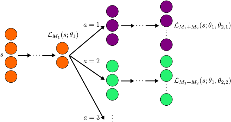
Figure 1: Schematic for alternating deep neural network (ADNN) model. The term ‘alternating’ refers to the estimation algorithm which cycles over the networks for each treatment $a\in\mathcal{A}$.

Algorithm 2 Alternating Deep Neural Networks

1:Tuning parameters $K_{1},K_{2}\in\mathbb{N}$, $\lambda\geq 0$; feature map dimension $r_{1}$; data $\left\{\overline{\mathbf{S}}_{i}^{T+1},\overline{\mbox{\bf A}}_{i}^{T},\overline{\mathbf{U}}^{T}_{i}\right\}_{i=1}^{n}$; batch size proportion $\nu\in(0,1)$; gradient-descent step-size $\left\{\alpha_{b}\right\}_{b\geq 1}$; error tolerance $\epsilon>0$; max number of iterations $N_{\max}$; and initial parameter values $\widehat{\theta}_{1,n}^{(1)},\widehat{\theta}_{2,n}^{(1)}$.

2:Set $D_{a}=\left\{(i,t)\,:\,A_{i}^{t}=a\right\}$ and $n_{a}=\#D_{a}$ for each $a\in\mathcal{A}$ and $t=1,\ldots,T$

3:for $b=1,\ldots,N_{\max}$ do

4:     for each $a\in\mathcal{A}$ do

5:         Draw a random batch $B_{a}$ of size $\lfloor\nu n_{a}\rfloor$ without replacement from $D_{a}$

6:         Compute a sub-gradient of the cost on batch $B_{a}$

$$\Lambda_{a}^{(b)}=\nabla\left[\frac{1}{\lfloor\nu n_{a}\rfloor}\sum_{(i,t)\in B_{a}}\big{|}\big{|}\mathcal{L}_{M_{1}+M_{2}}\left\{\mathbf{S}_{i}^{t};\widehat{\theta}_{1,n}^{(b)},\widehat{\theta}_{2,a,n}^{(b)}\right\}-\mbox{\bf Y}_{i}^{t+1}\big{|}\big{|}^{2}+\lambda\sum_{j=1}^{r_{1}}\sqrt{\sum_{\ell=1}^{r_{2}}\Sigma_{1,\ell,j}^{2}}\right]$$

7:         Compute a sub-gradient descent update

$$\left(\begin{array}[]{c}\widehat{\theta}_{1,n}^{(b+1)}\vskip 6.0pt plus 2.0pt minus 2.0pt\\ \widehat{\theta}_{2,a,n}^{(b+1)}\end{array}\right)=\left(\begin{array}[]{c}\widehat{\theta}_{1,n}^{(b)}\vskip 6.0pt plus 2.0pt minus 2.0pt\\ \widehat{\theta}_{2,a,n}^{(b)}\end{array}\right)+\alpha_{b}\Lambda_{a}^{(b)}$$

8:         Set $\widehat{\theta}_{2,a^{\prime},n}^{(b+1)}=\widehat{\theta}_{2,a^{\prime},n}^{(b)}$ for all $a^{\prime}\neq a$      

9:     If $\max_{a}\bigg{|}C_{n}^{\lambda}\left\{\widehat{\theta}_{1,n}^{(b+1)},\widehat{\theta}_{2,a,n}^{(b+1)}\right\}-C_{n}^{\lambda}\left\{\widehat{\theta}_{1,n}^{(b)},\widehat{\theta}_{2,a,n}^{(b)}\right\}\bigg{|}\leq\epsilon$ stop.

10:$\left(\widehat{\theta}_{1,n},\widehat{\theta}_{2,n}\right)=\left(\widehat{\theta}_{1,n}^{(b+1)},\widehat{\theta}_{2,n}^{(b+1)}\right)$

To select the dimension of the feature map we choose the lowest dimension for which the Brownian distance covariance test of independence between $\mbox{\bf Y}^{t+1}-\mathcal{L}_{M_{1}+M_{2}}(\mathbf{S}^{t};\widehat{\theta}_{1,n},\widehat{\theta}_{2,A^{t},n})$ and $\mathbf{S}^{t}$ fails to reject at a pre-specified error level $\tau\in(0,1)$. Let $\widehat{\phi}_{n}^{1}$ be the estimated feature map $\mbox{\bf s}\mapsto\mathcal{L}_{M_{1}}(\mbox{\bf s};\widehat{\theta}_{1})$. Define $\widehat{R}_{n}^{1}=\left\{j\in\left\{1,\ldots r_{1}\right\}\,:\,\widehat{\Sigma}_{1,\ell,j}^{2}\neq 0\,\mbox{for some}\,\ell\in\{1,\ldots,r_{2}\}\right\}$ to be the elements of $\mathbf{S}^{t}$ that dictate $\mathbf{S}_{\widehat{\phi}_{n}^{1}}^{t}$; write $\mathbf{S}_{\widehat{R}_{n}^{1}}^{t}$ as shorthand for $\left\{S^{t}_{j}\right\}_{j\in\widehat{R}_{n}^{1}}$. One may wish to iterate the foregoing estimation procedure as described in Corollary 3.3. However, because the components of $\mathbf{S}_{\widehat{\phi}_{n}^{1}}^{t}$ are each a potentially nonlinear combination of the elements of $\mathbf{S}_{\widehat{R}_{n}^{1}}^{t}$, therefore a sparse feature map defined on the domain of $\mathbf{S}_{\widehat{\phi}_{n}^{1}}^{t}$ may not be any more sparse in terms of the original features. Thus, when iterating the feature map construction algorithm, we recommend using the reduced process $\left\{\overline{\mathbf{S}}_{\widehat{R}_{n}^{1},i}^{T+1},\overline{\mbox{\bf A}}_{i}^{T},\overline{\mbox{\bf U}}_{i}^{T}\right\}_{i=1}^{n}$ and the input; because the sigma-algebra generated by $\mathbf{S}_{\widehat{R}_{n}^{1}}^{t}$ contains the sigma-algebra generated by $\mathbf{S}_{\widehat{\phi}_{n}^{1}}^{t}$, this does not incur any loss in generality. The above procedure can be iterated until no further dimension reduction occurs.

5 Simulation Experiments

We evaluate the finite sample performance of the proposed method (pre-screening with Brownian distance covariance + iterative alternating deep neural networks, which we will simply refer to as ADNN in this section) using a series of simulation experiments. To form a basis for comparison, we consider two alternative feature construction methods: (PCA) principal components analysis, so that the estimated feature map $\widehat{\phi}_{\mathrm{PCA}}(\mbox{\bf s})$ is the projection of s onto the first $k$ principal components of $T^{-1}\sum_{t=1}^{T}\mathbb{P}_{n}\left\{\mathbf{S}^{t}-\mathbb{P}_{n}\mathbf{S}^{t}\right\}\left\{\mathbf{S}^{t}-\mathbb{P}_{n}\mathbf{S}^{t}\right\}^{\intercal}$; and (tNN) a traditional sparse neural network, which can be seen as a special case of our proposed alternating deep neural network estimator where there is only 1 action. In our implementation of PCA, we choose the number of principal components, $k$, corresponding to 90% of variance explained. We do not compare with sparse PCA for variable selection, because based on preliminary runs, the principal components that explain 50% of variance already use all the variables in our generative model. In our implementation of tNN, we build a separate tNN for each $a\in\mathcal{A}$, where $(\lambda,K_{1},K_{2},r_{1})$ are tuned using cross-validation, and take the union of selected variables and constructed features. Note that there is no other obvious way to join the constructed features from tNN but to simply concatenate them, which will lead to inefficient dimension reduction especially when $|\mathcal{A}|$ is large, whereas we will see that ADNN provides a much more efficient way to aggregate the useful information across actions.

We evaluate the quality of a feature map, $\phi$, in terms of the marginal mean outcome under the estimated optimal regime constructed from the reduced data $\left\{\overline{\mathbf{S}}_{i}^{T+1},\overline{\mbox{\bf A}}_{i}^{T},\overline{\mbox{\bf U}}_{i}^{T}\right\}_{i=1}^{n}$ using Q-learning with function approximation (Bertsekas and Tsitsiklis, 1996; Murphy, 2005); we use both linear function approximation and non-linear function approximation with neural networks. A description of Q-learning as well as these approximation architectures are described in the Supplemental Materials.

We consider data from the following class of generative models, as illustrated in Figure 2:

$$\mathbf{S}^{1}\sim\mathrm{Normal}_{64}\left(0,\;0.25\mathbf{I}_{64}\right);\quad A^{1},\ldots,A^{T}\sim_{i.i.d.}\mathrm{Bernoulli}\left(0.5\right);$$

$$S^{t+1}_{4i-3},S^{t+1}_{4i-2}\sim_{i.i.d.}\mathrm{Normal}\left\{(1-A^{t})g(S_{i}^{t}),\;0.01(1-A^{t})+0.25A^{t}\right\};$$

$$S^{t+1}_{4i-1},S^{t+1}_{4i}\sim_{i.i.d.}\mathrm{Normal}\left\{A^{t}g(S_{i}^{t}),\;0.01A^{t}+0.25(1-A^{t})\right\};$$

$$U^{t}\sim\mathrm{Normal}\{(1-A^{t})[2\{g(S^{t}_{1})+g(S_{2}^{t})\}-\{g(S_{3}^{t})+g(S_{4}^{t})\}]$$

$$\qquad\qquad\qquad+A^{t}[2\{g(S^{t}_{3})+g(S_{4}^{t})\}-\{g(S_{1}^{t})+g(S_{2}^{t})\}],\;0.01\};$$

$$\text{for}\;i=1,2,\ldots,16.$$

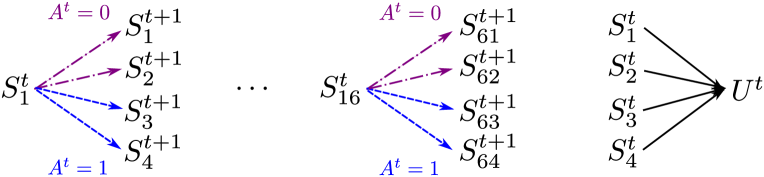
Figure 2: Relationship between $\mathbf{S}^{t}$ and $\mathbf{Y}^{t+1}$ in the generative model, which depends on the action. First 16 variables determine the next state. First 4 variables determine the utility.

The above class of models is indexed by $g:\mathbb{R}\rightarrow\mathbb{R}$ which we vary across the following maps: identity $g(u)=u$, truncated quadratic $g(u)=\min\{u^{2},3\}$, and truncated exponential $g(u)=\min\{\exp(u),3\}$, where the truncation is used to keep all variables of relatively the same scale across time points. Additionally, we add 3 types of noise variables, each taking up about $\frac{1}{3}$ of total noises added: (i) dependent noise variables $D^{t}_{j}$, which are generated the same way as above except that they don’t affect the utility; (ii) white noises $W^{t}_{k}$, which are sampled independently from $\mathrm{Normal}(0,0.25)$ at each time point; and (iii) constants $C^{t}_{l}$, which are sampled independently from $\mathrm{Normal}(0,0.25)$ at $t=1$ and remain constant over time. More precisely, let $m$ be the total number of noise variables, then

$$D^{1}_{j},W^{1}_{k},C^{1}_{l}\sim_{i.i.d.}\mathrm{Normal}\left(0,0.25\right);$$

$$D^{t+1}_{4i-3},D^{t+1}_{4i-2}\sim_{i.i.d.}\mathrm{Normal}\left\{(1-A^{t})g(D_{i}^{t}),\;0.01(1-A^{t})+0.25A^{t}\right\};$$

$$D^{t+1}_{4i-1},D^{t+1}_{4i}\sim_{i.i.d.}\mathrm{Normal}\left\{A^{t}g(D_{i}^{t}),\;0.01A^{t}+0.25(1-A^{t})\right\};$$

$$W^{t}_{k}\sim_{i.i.d.}\mathrm{Normal}\left(0,0.25\right);\;C^{t}_{l}=C^{1}_{l};$$

$$\text{for}\;j=1,2,\ldots,\lfloor m/3\rfloor;k=1,2,\ldots,\lceil m/3\rceil;l=1,2,\ldots,\lceil m/3\rceil.$$

It can be seen that the first 16 variables, the first 4 variables, and $\{g(S_{1}^{t}),g(S_{2}^{t}),g(S_{3}^{t})+g(S_{4}^{t})\}^{\intercal}$ all induce a sufficient MDP. the foregoing class of models is designed to evaluate the ability of the proposed method to identify low-dimensional and potentially nonlinear features of the state in the presence of action-dependent transitions and various noises. For each Monte Carlo replication, we sample $n=30$ i.i.d. trajectories of length $T=90$ from the above generative model.

The results based on 500 Monte Carlo replications are reported in Table 1 - 3. In addition to reporting the marginal mean outcome under the policy estimated using Q-learning with both function approximations, we also report: (nVar) the number of selected variables; and (nDim) the dimension of the feature map. The table shows that (i) ADNN produces substantially smaller nVar and nDim compared with PCA or tNN in all cases; (ii) ADNN is robust to the 3 types of noises; (iii) when fed into the Q-learning algorithm, ADNN leads to considerably better marginal mean outcome than PCA and the original states under non-linear models; and (iv) ADNN is able to construct features suitable for Q-learning with linear function approximation even when the utility function and transition between states are non-linear.

Model	nNoise	Feature map	Linear Q	NNQ	nVar	nDim
linear	0	$\mbox{\bf s}_{t}$	3.36(0.012)	3.31(0.012)	64	64
		$(s_{1}^{t},s_{2}^{t},s_{3}^{t},s_{4}^{t})^{\intercal}$	3.34(0.012)	3.31(0.013)	4	4
		$\widehat{\phi}_{\text{ADNN}}(\mbox{\bf s}^{t})$	3.21(0.018)	3.34(0.013)	4.1(0.01)	3.1(0.02)
		$\widehat{\phi}_{\text{tNN}}(\mbox{\bf s}^{t})$	3.38(0.012)	3.30(0.012)	16.0(0.00)	34.4(0.13)
		$\widehat{\phi}_{\text{PCA}}(\mbox{\bf s}^{t})$	3.34(0.012)	3.30(0.012)	64	50.0(0.00)
	50	$\mbox{\bf s}_{t}$	3.31(0.012)	3.27(0.012)	114	114
		$(s_{1}^{t},s_{2}^{t},s_{3}^{t},s_{4}^{t})^{\intercal}$	3.31(0.012)	3.29(0.013)	4	4
		$\widehat{\phi}_{\text{ADNN}}(\mbox{\bf s}^{t})$	3.26(0.014)	3.32(0.013)	5.6(0.08)	4.6(0.08)
		$\widehat{\phi}_{\text{tNN}}(\mbox{\bf s}^{t})$	3.32(0.012)	3.29(0.013)	37.0(0.00)	86.0(0.19)
		$\widehat{\phi}_{\text{PCA}}(\mbox{\bf s}^{t})$	3.34(0.012)	3.28(0.013)	114	85.8(0.02)
	200	$\mbox{\bf s}_{t}$	2.17(0.016)	2.98(0.035)	264	264
		$(s_{1}^{t},s_{2}^{t},s_{3}^{t},s_{4}^{t})^{\intercal}$	3.33(0.012)	3.31(0.013)	4	4
		$\widehat{\phi}_{\text{ADNN}}(\mbox{\bf s}^{t})$	3.29(0.013)	3.32(0.012)	10.2(0.12)	7.5(0.09)
		$\widehat{\phi}_{\text{tNN}}(\mbox{\bf s}^{t})$	3.34(0.012)	3.27(0.013)	87.4(0.11)	157.8(0.48)
		$\widehat{\phi}_{\text{PCA}}(\mbox{\bf s}^{t})$	3.33(0.013)	3.11(0.028)	264	166.0(0.02)

Table 1: Comparison of feature map estimators under linear transition and different number of noise variables (nNoise) in terms of: marginal mean outcome using Q-learning with linear function approximation (Linear Q); Q-learning with neural network function approximation (NN Q); the number of selected variables (nVar); and the dimension of the feature map (nDim)

Model	nNoise	Feature map	Linear Q	NNQ	nVar	nDim
quad	0	$\mbox{\bf s}_{t}$	3.08(0.062)	2.64(0.073)	64	64
		$(s_{1}^{t},s_{2}^{t},s_{3}^{t},s_{4}^{t})^{\intercal}$	2.54(0.056)	6.75(0.046)	4	4
		$\widehat{\phi}_{\text{ADNN}}(\mbox{\bf s}^{t})$	6.63(0.038)	6.97(0.034)	4.1(0.02)	2.4(0.04)
		$\widehat{\phi}_{\text{tNN}}(\mbox{\bf s}^{t})$	6.94(0.027)	6.54(0.068)	15.3(0.04)	37.1(0.22)
		$\widehat{\phi}_{\text{PCA}}(\mbox{\bf s}^{t})$	2.97(0.064)	2.50(0.067)	64	51.2(0.02)
	50	$\mbox{\bf s}_{t}$	2.96(0.054)	1.69(0.064)	114	114
		$(s_{1}^{t},s_{2}^{t},s_{3}^{t},s_{4}^{t})^{\intercal}$	2.58(0.057)	6.76(0.042)	4	4
		$\widehat{\phi}_{\text{ADNN}}(\mbox{\bf s}^{t})$	6.76(0.032)	6.99(0.030)	6.4(0.06)	5.3(0.09)
		$\widehat{\phi}_{\text{tNN}}(\mbox{\bf s}^{t})$	6.98(0.031)	6.53(0.064)	36.5(0.03)	88.3(0.22)
		$\widehat{\phi}_{\text{PCA}}(\mbox{\bf s}^{t})$	3.09(0.061)	2.00(0.067)	114	87.1(0.03)
	200	$\mbox{\bf s}_{t}$	1.28(0.030)	0.88(0.031)	264	264
		$(s_{1}^{t},s_{2}^{t},s_{3}^{t},s_{4}^{t})^{\intercal}$	2.52(0.056)	6.68(0.050)	4	4
		$\widehat{\phi}_{\text{ADNN}}(\mbox{\bf s}^{t})$	6.87(0.034)	6.92(0.033)	14.3(0.14)	12.5(0.23)
		$\widehat{\phi}_{\text{tNN}}(\mbox{\bf s}^{t})$	6.76(0.044)	6.03(0.075)	84.1(0.11)	152.4(0.36)
		$\widehat{\phi}_{\text{PCA}}(\mbox{\bf s}^{t})$	3.09(0.062)	0.96(0.033)	264	167.4(0.03)

Table 2: Comparison of feature map estimators under quadratic transition

Model	nNoise	Feature map	Linear Q	NNQ	nVar	nDim
exp	0	$\mbox{\bf s}_{t}$	8.73(0.008)	8.78(0.012)	64	64
		$(s_{1}^{t},s_{2}^{t},s_{3}^{t},s_{4}^{t})^{\intercal}$	9.20(0.006)	9.43(0.004)	4	4
		$\widehat{\phi}_{\text{ADNN}}(\mbox{\bf s}^{t})$	9.30(0.018)	9.45(0.004)	4.3(0.13)	2.4(0.13)
		$\widehat{\phi}_{\text{tNN}}(\mbox{\bf s}^{t})$	9.44(0.005)	9.29(0.009)	16.0(0.00)	42.3(0.17)
		$\widehat{\phi}_{\text{PCA}}(\mbox{\bf s}^{t})$	9.10(0.016)	9.02(0.023)	64	14.2(0.018)
	50	$\mbox{\bf s}_{t}$	8.78(0.008)	8.77(0.012)	114	114
		$(s_{1}^{t},s_{2}^{t},s_{3}^{t},s_{4}^{t})^{\intercal}$	9.19(0.006)	9.43(0.005)	4	4
		$\widehat{\phi}_{\text{ADNN}}(\mbox{\bf s}^{t})$	9.32(0.018)	9.43(0.005)	5.4(0.03)	2.4(0.04)
		$\widehat{\phi}_{\text{tNN}}(\mbox{\bf s}^{t})$	9.43(0.005)	9.18(0.012)	37.0(0.00)	81.5(0.28)
		$\widehat{\phi}_{\text{PCA}}(\mbox{\bf s}^{t})$	8.89(0.014)	8.99(0.020)	114	37.2(0.02)
	200	$\mbox{\bf s}_{t}$	8.71(0.008)	8.73(0.012)	264	264
		$(s_{1}^{t},s_{2}^{t},s_{3}^{t},s_{4}^{t})^{\intercal}$	9.19(0.006)	9.44(0.004)	4	4
		$\widehat{\phi}_{\text{ADNN}}(\mbox{\bf s}^{t})$	9.37(0.016)	9.41(0.006)	7.8(0.09)	3.3(0.12)
		$\widehat{\phi}_{\text{tNN}}(\mbox{\bf s}^{t})$	9.41(0.005)	9.06(0.016)	93.4(0.10)	152.4(0.42)
		$\widehat{\phi}_{\text{PCA}}(\mbox{\bf s}^{t})$	8.66(0.014)	9.02(0.022)	264	91.4(0.02)

Table 3: Comparison of feature map estimators under exponential transition

6 Application to BASICS-Mobile

We illustrate the proposed methedology using data on the effectiveness of BASICS-Mobile, a behavioral intervention delivered via mobile device, targeting heavy drinking and smoking among college students (Witkiewitz et al., 2014). Mobile interventions are appealing because of their 24-hour availability, anonymity, portability, increased compliance, and accurate data recording (Heron and Smyth, 2010). BASICS-Mobile enrolled 30 students and lasted for 14 days. On the afternoon and evening of each day, the student is asked to complete a list of self-report questions, and then either an informational module or a treatment module is provided. A treatment module contains 1-3 mobile phone screens of interactive content, such as comparing the student’s smoking level with the levels of their peers, or guiding the student to manage their smoking urges. A treatment module is generally more burdensome than an informational module, and may be less effective if, for example, the student’s stress level is high; furthermore, excessive treatment can cause habituation and disengagement from the intervention. An optimal intervention will assignment a treatment module if and when it is needed without diminishing engagement.

In our original formulation of this decision problem as an MDP, the state comprises of 15 variables capturing baseline information, current answers to the self-report questions, a weekend indicator, age, past attempts to quit smoking, current smoking urge, and current stress level; the action is whether a treatment module gets assigned; the reward is the negative of the cigarettes smoked at the next time point; the goal is to find a strategy that minimizes cumulative cigarette rate.

Two students with large amounts of missing data are excluded. All other missing values are imputed with the fitted value from a local polynomial regression of the state variable on time $t$. We treat all the variables as ordinal, partitioning some of them (see the Supplemental Materials for a complete description). We estimate $\widehat{\phi}_{\text{ADNN}}(s_{t})$ wherein conditional independence is checked via condition (i) in Lemma 3.4. The dimension of $\widehat{\phi}_{\text{ADNN}}(s_{t})$ is set to be the smallest dimension for which $\widehat{\phi}_{\text{ADNN}}(s_{t})$ fails to reject this independence condition at level $\tau=0.05$; this procedure resulted in a feature of dimension six. To increase the interpretability of the constructed feature map, we constrained the dimension reduction network to have no hidden layers. Under this constraint, $\widehat{\phi}_{\text{ADNN}}(s_{t})$ is a linear transformation of $s_{t}$ followed by application of $\Phi^{\circ}$ which was set to be the arctangent function. A plot of the weights of the 15 original variables in the linear transformation for each component of the feature map is useful in interpreting the learned feature map; see Figure 3 for an example.

Figure 3: Weights of the original variables in the first two components of the estimated feature map.

We estimate the optimal strategy using Q-learning applied to the learned feature map. Comparing the estimated parameters for treatment and no treatment, while examining the plots of weights, we can give a sense of how the original variables impact the optimal treatment assignment. For instance, the 1st parameter in the Q-function for treatment is smaller than the one for no treatment, which suggests that the 1st new variable contributes to the decision to apply treatment by being small, i.e., if it is the weekend and a student’s stress level is low then the estimated policy is more likely to provide treatment. This agrees with the intuition that a treatment module would be more effective when the student is not busy or stressed. Similarly, it can be seen that previous attempts to quit smoking is positively associated with providing treatment, with the possible explanation that individuals with prior quit attempts tend to be more severe and in need of frequent treatment.

7 Discussion

Data-driven decision support systems are being deployed across a wide range of application domains including medicine, engineering, and business. MDPs provide the mathematical underpinning for most data-driven decision problems with an infinite or indefinite time horizon. While the MDP model is extremely general, choosing a parsimonious representation of a decision process that fits the MDP model is non-trivial. We introduced the notion of a feature map which induces a sufficient MDP and provided an estimator of such a feature map based on a variant of deep neural networks.

There are several important ways in which this work can be extended; we mention two of the most pressing here. We considered estimation from a batch of i.i.d. replicates; however, in some applications it may be desirable to estimate a feature map online as data accumulate. In such cases, a data-driven, and hence evolving, feature map of the state will be stored complicating estimation. Furthermore, because the proposed algorithm sweeps through the observed data multiple times it is not suitable for real-time estimation. Another important extension is to states with complex data structures, e.g., images and text, such data are increasingly common in health, engineering, and security applications. Existing neural network architectures designed for such data (Krizhevsky et al., 2012; Dahl et al., 2012; Simonyan and Zisserman, 2014) could potentially be integrated into the proposed feature map construction algorithm.

8 Supplemental Materials

Q-learning

Let $(\overline{\mathbf{A}}^{t},\overline{\mathbf{S}}^{t+1},\overline{\mathbf{U}}^{t})$ be an MDP. The value of a state-action pair under a policy $\pi$, referred to as the Q-function, is the discounted mean utility if the current state is $\mathbf{s}$, current action is $a$, and the agent follows $\pi$ afterwards: $Q^{\pi}(\mathbf{s},a)=\mathbb{E}\left\{\sum_{t\geq 1}\gamma^{t-1}U^{*t}(\pi)\lvert\mathbf{S}^{1}=\mathbf{s},A^{1}=a\right\}$, where $\gamma\in(0,1)$ is the discount factor. An optimal policy $\pi^{\text{opt}}$ yields the largest value for every state-action pair. Denote the corresponding Q-function as $Q^{\text{opt}}(\mathbf{s},a)=Q^{\pi^{\text{opt}}}(\mathbf{s},a)=\underset{\pi}{\max}\;Q^{\pi}(\mathbf{s},a)$. If $Q^{\text{opt}}(\mathbf{s},a)$ is known for all $(\mathbf{s},a)$, then an optimal policy can be defined as $\pi^{\text{opt}}(\mbox{\bf s})=\underset{a\in\mathcal{A}}{\text{argmax}}\;Q^{\text{opt}}(\mathbf{s},a).$ $Q^{\text{opt}}$ satisfies the Bellman Optimality Equations (BOE):

$$Q^{\text{opt}}(\mathbf{s},a)=\mathbb{E}\left\{U^{t}+\gamma\;\underset{a^{\prime}\in\mathcal{A}}{\max}\;Q^{\text{opt}}(\mathbf{S}^{t+1},a^{\prime})\;\lvert\;\mathbf{S}^{t}=\mbox{\bf s},A^{t}=a\right\}.$$

In practice, one often cannot obtain $Q^{\text{opt}}$ by solving the above equations, because computing the right-hand-side requires the underlying model of the MDP, which is often unknown. Besides, solving a huge linear system can be costly.

Q-learning is a stochastic optimization algorithm that doesn’t require knowing the transition model or solving a linear system. The update step for the classic Q-learning, Watkin’s Q-learning (Sutton and Barto, 1998), for finite state and action spaces, is as follows:

$$Q^{k+1}(\mathbf{s}_{t},a_{t})\leftarrow Q^{k}(\mathbf{s}_{t},a_{t})+\alpha\{u_{t}+\gamma\,\underset{a}{\max}\;Q^{k}(\mathbf{s}_{t+1},a)-Q^{k}(\mathbf{s}_{t},a_{t})\},$$

where $\alpha$ is the learning rate. If the state space is continuous, one may approximate $Q(\mathbf{s},a)$ with a parametric function $F(\mathbf{s},a;\boldsymbol{\theta})$ and update the parameters instead:

$$\boldsymbol{\theta}^{k+1}\leftarrow\boldsymbol{\theta}^{k}+\alpha\{u_{t}+\gamma\;\underset{a}{\max}\;F(\mathbf{s}_{t+1},a;\boldsymbol{\theta}^{k})-F(\mathbf{s}_{t},a_{t};\boldsymbol{\theta}^{k})\}\cdot\nabla_{\!\boldsymbol{\theta}}F(\mathbf{s}_{t},a_{t};\boldsymbol{\theta}^{k}).$$

Proof of Theorem 3.2

Proof.

First we show that the process $(\overline{\mathbf{A}}^{t},\overline{\mathbf{S}}^{t+1}_{\phi},\overline{\mathbf{U}}^{t})$ induced by $(\phi,\Pi_{\phi,msbl})$ satisfies (SM1). For any $t\in\mathbb{N}$ and measurable subset $\mathcal{G}\in\mathbb{R}^{q}$,

$$P(\mathbf{S}_{\phi}^{t+1}\in\mathcal{G}_{\phi}^{t+1}\lvert\overline{\mathbf{S}}_{\phi}^{t},\overline{\mbox{\bf A}}^{t})$$

$$= \mathbb{E}\{P(\mathbf{S}_{\phi}^{t+1}\in\mathcal{G}_{\phi}^{t+1}\lvert\mathbf{S}^{t},\overline{\mathbf{S}}_{\phi}^{t},\overline{\mbox{\bf A}}^{t})\lvert\overline{\mathbf{S}}_{\phi}^{t},\overline{\mbox{\bf A}}^{t}\}$$

$$= \mathbb{E}\{P(\mathbf{S}_{\phi}^{t+1}\in\mathcal{G}_{\phi}^{t+1}\lvert\mathbf{S}^{t},\mathbf{S}_{\phi}^{t},A^{t})\lvert\overline{\mathbf{S}}_{\phi}^{t},\overline{\mbox{\bf A}}^{t}\}\quad(\text{by Markov property of the original process})$$

$$= \mathbb{E}\{P(\mathbf{S}_{\phi}^{t+1}\in\mathcal{G}_{\phi}^{t+1}\lvert\mathbf{S}_{\phi}^{t},A^{t})\lvert\overline{\mathbf{S}}_{\phi}^{t},\overline{\mbox{\bf A}}^{t}\}\quad(\text{by (\ref{sufficientTheoremCond1})})$$

$$= P(\mathbf{S}^{t+1}_{\phi}\in\mathcal{G}_{\phi}^{t+1}\lvert\mathbf{S}^{t}_{\phi},A^{t})$$

Also note that $\mathbb{E}\{P(\mathbf{S}_{\phi}^{t+1}\in\mathcal{G}_{\phi}^{t+1}\lvert\mathbf{S}^{t},\overline{\mathbf{S}}_{\phi}^{t},\overline{\mbox{\bf A}}^{t})\lvert\overline{\mathbf{S}}_{\phi}^{t},\overline{\mbox{\bf A}}^{t}\}$ does not depend on $t$ by homogeneity of the original process. Thus the induced process is Markov and homogeneous.

Next we show that the induced process satisfies (SM2). Let $Q^{\text{opt}}(\mathbf{s},a)$ be defined as before. Then we have

$$Q^{\text{opt}}(\mathbf{s},a) =\text{E}[U^{t}+\gamma\;\underset{a^{\prime}}{\max}\;Q^{\text{opt}}(\mathbf{S}^{t+1},a^{\prime})\;\lvert\;\mathbf{S}^{t}=\mathbf{s},A^{t}=a]\quad(\text{by BOE})$$

$$=\text{E}[U^{t}+\gamma\;\underset{a^{\prime}}{\max}\;Q^{\text{opt}}(\mathbf{S}^{t+1},a^{\prime})\;\lvert\;\mathbf{S}^{t}=\mathbf{s},\mathbf{S}^{t}_{\phi}=\mathbf{s}_{\phi},A^{t}=a]$$

$$=\text{E}[U^{t}+\gamma\;\underset{a^{\prime}}{\max}\;Q^{\text{opt}}(\mathbf{S}^{t+1},a^{\prime})\;\lvert\;\mathbf{S}^{t}_{\phi}=\mathbf{s}_{\phi},A^{t}=a]\quad(\text{by (2)})$$

$$=Q_{\phi}^{\text{opt}}(\mathbf{s}_{\phi},a),\quad\text{and}$$

$$\pi^{\text{opt}}(\mathbf{s})=\underset{a}{\text{argmax}}\;Q^{\text{opt}}(\mathbf{s},a)=\underset{a}{\text{argmax}}\;Q_{\phi}^{\text{opt}}(\mathbf{s}_{\phi},a)=\pi_{\phi}^{\text{opt}}(\mathbf{s}_{\phi}).$$

∎

Proof of Corollary 3.3

Proof.

By assumption $(\phi_{0},\Pi_{\phi_{0},\text{msrbl}})$ induces a sufficient MDP for $\pi^{\text{opt}}$ within $\Pi_{\text{msrbl}}$, then by definition the process $(\overline{\mathbf{A}}^{t},\overline{\mathbf{S}}^{t+1}_{\phi_{0}},\overline{\mathbf{U}}^{t})$ is Markov and homogeneous, and there exists $\pi^{\text{opt}}=\pi_{\phi_{0}}^{\text{opt}}\circ\phi_{0}$.

Define $\overline{\phi}_{k}=\phi_{k}\circ\cdots\circ\phi_{0}$. By (3) and Theorem 3.2, $(\phi_{1},\Pi_{\phi_{1},\text{msrbl}})$ induces a sufficient MDP for $\pi_{\phi_{0}}^{\text{opt}}$ within $\Pi_{\phi_{0},\text{msrbl}}$. Then the process $(\overline{\mathbf{A}}^{t},\overline{\mathbf{S}}_{\overline{\phi}_{1}},\overline{\mathbf{U}}^{t})$ is Markov and homogeneous, and there exists $\pi^{\text{opt}}_{\phi_{0}}=\pi^{\text{opt}}_{\overline{\phi}_{1}}\circ\phi_{1}$. Thus $\pi^{\text{opt}}=\pi_{\phi_{0}}^{\text{opt}}\circ\phi_{0}=\pi^{\text{opt}}_{\overline{\phi}_{1}}\circ\overline{\phi}_{1}$. Therefore $(\overline{\phi}_{1},\Pi_{\overline{\phi}_{1},\text{msrbl}})$ induces a sufficient MDP for $\pi^{\text{opt}}$ within $\Pi_{\text{msrbl}}.$ ∎

Proof of Lemma 3.4

Proof.

We show that (i) $\Rightarrow\mathbf{Y}^{t+1}\mathchoice{\mathrel{\hbox to0.0pt{$\displaystyle\perp$\hss}\mkern 2.0mu{\displaystyle\perp}}}{\mathrel{\hbox to0.0pt{$\textstyle\perp$\hss}\mkern 2.0mu{\textstyle\perp}}}{\mathrel{\hbox to0.0pt{$\scriptstyle\perp$\hss}\mkern 2.0mu{\scriptstyle\perp}}}{\mathrel{\hbox to0.0pt{$\scriptscriptstyle\perp$\hss}\mkern 2.0mu{\scriptscriptstyle\perp}}}\mathbf{S}^{t}\lvert\mathbf{S}_{\phi}^{t},A^{t}$:

$$\{\mathbf{Y}^{t+1}-\mathbb{E}(\mbox{\bf Y}^{t+1}\lvert\mathbf{S}_{\phi}^{t},A^{t})\}\mathchoice{\mathrel{\hbox to0.0pt{$\displaystyle\perp$\hss}\mkern 2.0mu{\displaystyle\perp}}}{\mathrel{\hbox to0.0pt{$\textstyle\perp$\hss}\mkern 2.0mu{\textstyle\perp}}}{\mathrel{\hbox to0.0pt{$\scriptstyle\perp$\hss}\mkern 2.0mu{\scriptstyle\perp}}}{\mathrel{\hbox to0.0pt{$\scriptscriptstyle\perp$\hss}\mkern 2.0mu{\scriptscriptstyle\perp}}}\mathbf{S}^{t}\lvert A^{t}$$

$$\Rightarrow \{\mathbf{Y}^{t+1}-\mathbb{E}(\mbox{\bf Y}^{t+1}\lvert\mathbf{S}_{\phi}^{t},A^{t})\}\mathchoice{\mathrel{\hbox to0.0pt{$\displaystyle\perp$\hss}\mkern 2.0mu{\displaystyle\perp}}}{\mathrel{\hbox to0.0pt{$\textstyle\perp$\hss}\mkern 2.0mu{\textstyle\perp}}}{\mathrel{\hbox to0.0pt{$\scriptstyle\perp$\hss}\mkern 2.0mu{\scriptstyle\perp}}}{\mathrel{\hbox to0.0pt{$\scriptscriptstyle\perp$\hss}\mkern 2.0mu{\scriptscriptstyle\perp}}}(\mathbf{S}^{t},\mathbf{S}_{\phi}^{t})\lvert A_{t}$$

$$\Rightarrow \{\mathbf{Y}^{t+1}-\mathbb{E}(\mbox{\bf Y}^{t+1}\lvert\mathbf{S}_{\phi}^{t},A^{t})\}\mathchoice{\mathrel{\hbox to0.0pt{$\displaystyle\perp$\hss}\mkern 2.0mu{\displaystyle\perp}}}{\mathrel{\hbox to0.0pt{$\textstyle\perp$\hss}\mkern 2.0mu{\textstyle\perp}}}{\mathrel{\hbox to0.0pt{$\scriptstyle\perp$\hss}\mkern 2.0mu{\scriptstyle\perp}}}{\mathrel{\hbox to0.0pt{$\scriptscriptstyle\perp$\hss}\mkern 2.0mu{\scriptscriptstyle\perp}}}\mathbf{S}^{t}\lvert\mathbf{S}_{\phi}^{t},A^{t}$$

$$\Rightarrow \mathbf{Y}^{t+1}\mathchoice{\mathrel{\hbox to0.0pt{$\displaystyle\perp$\hss}\mkern 2.0mu{\displaystyle\perp}}}{\mathrel{\hbox to0.0pt{$\textstyle\perp$\hss}\mkern 2.0mu{\textstyle\perp}}}{\mathrel{\hbox to0.0pt{$\scriptstyle\perp$\hss}\mkern 2.0mu{\scriptstyle\perp}}}{\mathrel{\hbox to0.0pt{$\scriptscriptstyle\perp$\hss}\mkern 2.0mu{\scriptscriptstyle\perp}}}\mathbf{S}^{t}\lvert\mathbf{S}_{\phi}^{t},A^{t}.$$

The 1st implication follows from the fact that $\mathbf{S}_{\phi}^{t}$ is a transformation of $\mathbf{S}^{t}$. The 2nd implication follows from the fact that $X\mathchoice{\mathrel{\hbox to0.0pt{$\displaystyle\perp$\hss}\mkern 2.0mu{\displaystyle\perp}}}{\mathrel{\hbox to0.0pt{$\textstyle\perp$\hss}\mkern 2.0mu{\textstyle\perp}}}{\mathrel{\hbox to0.0pt{$\scriptstyle\perp$\hss}\mkern 2.0mu{\scriptstyle\perp}}}{\mathrel{\hbox to0.0pt{$\scriptscriptstyle\perp$\hss}\mkern 2.0mu{\scriptscriptstyle\perp}}}Y,Z\Rightarrow f(X\lvert Y,Z)=f(X)=f(X\lvert Z)\Rightarrow X\mathchoice{\mathrel{\hbox to0.0pt{$\displaystyle\perp$\hss}\mkern 2.0mu{\displaystyle\perp}}}{\mathrel{\hbox to0.0pt{$\textstyle\perp$\hss}\mkern 2.0mu{\textstyle\perp}}}{\mathrel{\hbox to0.0pt{$\scriptstyle\perp$\hss}\mkern 2.0mu{\scriptstyle\perp}}}{\mathrel{\hbox to0.0pt{$\scriptscriptstyle\perp$\hss}\mkern 2.0mu{\scriptscriptstyle\perp}}}Y\lvert Z$ for random variables $X,Y,$ and $Z$. The 3rd implication follows from the fact that $\mathbb{E}(\mbox{\bf Y}^{t+1}\lvert\mathbf{S}_{\phi}^{t},A^{t})$ is constant conditional on $\mathbf{S}^{t}_{\phi}$ and $A^{t}$.

Similarly, one can show that (ii) $\Rightarrow\mathbf{Y}^{t+1}\mathchoice{\mathrel{\hbox to0.0pt{$\displaystyle\perp$\hss}\mkern 2.0mu{\displaystyle\perp}}}{\mathrel{\hbox to0.0pt{$\textstyle\perp$\hss}\mkern 2.0mu{\textstyle\perp}}}{\mathrel{\hbox to0.0pt{$\scriptstyle\perp$\hss}\mkern 2.0mu{\scriptstyle\perp}}}{\mathrel{\hbox to0.0pt{$\scriptscriptstyle\perp$\hss}\mkern 2.0mu{\scriptscriptstyle\perp}}}\mathbf{S}^{t}\lvert\mathbf{S}_{\phi}^{t},A^{t}$. ∎

Proof of Theorem 3.5

Proof.

First we show that the process $(\overline{\mathbf{A}}^{t},\overline{\mathbf{S}}^{t+1}_{\phi},\overline{\mathbf{U}}^{t})$ induced by $(\phi,\Pi_{\phi,msbl})$ satisfies (SM1). For any $t\in\mathbb{N}$ and measurable subset $\mathcal{G}\in\mathbb{R}^{q}$,

$$P(\mathbf{S}_{\phi}^{t+1}\in\mathcal{G}_{\phi}^{t+1}\lvert\overline{\mathbf{S}}_{\phi}^{t},\overline{\mbox{\bf A}}^{t})$$

$$= \mathbb{E}\{P(\mathbf{S}_{\phi}^{t+1}\in\mathcal{G}_{\phi}^{t+1}\lvert\mathbf{S}^{t},\overline{\mathbf{S}}_{\phi}^{t},\overline{\mbox{\bf A}}^{t})\lvert\overline{\mathbf{S}}_{\phi}^{t},\overline{\mbox{\bf A}}^{t}\}$$

$$= \mathbb{E}\{P(\mathbf{S}_{\phi}^{t+1}\in\mathcal{G}_{\phi}^{t+1}\lvert\mathbf{S}^{t},\mathbf{S}_{\phi}^{t},A^{t})\lvert\overline{\mathbf{S}}_{\phi}^{t},\overline{\mbox{\bf A}}^{t}\}\quad(\text{by Markov property of the original process})$$

$$= \mathbb{E}\{P(\mathbf{S}_{\phi}^{t+1}\in\mathcal{G}_{\phi}^{t+1}\lvert\mathbf{S}_{\phi}^{t},A^{t})\lvert\overline{\mathbf{S}}_{\phi}^{t},\overline{\mbox{\bf A}}^{t}\}\quad(\text{by (\ref{sufficientTheoremCond2})})$$

$$= P(\mathbf{S}^{t+1}_{\phi}\in\mathcal{G}_{\phi}^{t+1}\lvert\mathbf{S}^{t}_{\phi},A^{t})$$

Also note that $\mathbb{E}\{P(\mathbf{S}_{\phi}^{t+1}\in\mathcal{G}_{\phi}^{t+1}\lvert\mathbf{S}^{t},\overline{\mathbf{S}}_{\phi}^{t},\overline{\mbox{\bf A}}^{t})\lvert\overline{\mathbf{S}}_{\phi}^{t},\overline{\mbox{\bf A}}^{t}\}$ does not depend on $t$ by homogeneity of the original process. Thus the induced process is Markov and homogeneous.

Next we show that the induced process satisfies (SM2). Define

$$Q^{\text{opt},1}(\mbox{\bf s}^{t},a^{t}):= \mathbb{E}\{U(\mathbf{S}^{t},A^{t},\mathbf{S}^{t+1})\;\lvert\;\mathbf{S}^{t}=\mathbf{s}^{t},A^{t}=a^{t}\}$$

$$= \mathbb{E}\{U(\mathbf{S}_{\phi}^{t},A^{t},\mathbf{S}_{\phi}^{t+1})\;\lvert\;\mathbf{S}^{t}=\mbox{\bf s}^{t},A^{t}=a^{t}\}\quad\text{(by (\ref{sufficientTheoremCond2}))}$$

$$= \mathbb{E}\{U(\mathbf{S}_{\phi}^{t},A^{t},\mathbf{S}_{\phi}^{t+1})\;\lvert\;\mathbf{S}_{\phi}^{t}=\mbox{\bf s}_{\phi}^{t},A^{t}=a^{t}\}$$

$$= Q^{\text{opt},1}_{\phi}(\mbox{\bf s}^{t}_{\phi},a^{t})$$

For $T\geq 2$, define

$$Q^{\text{opt},T}(\mbox{\bf s}^{t},a^{t}):= \mathbb{E}\{U(\mathbf{S}^{t},A^{t},\mathbf{S}^{t+1})+\gamma\;\underset{a^{\prime}}{\max}\;Q^{\text{opt},T-1}(\mathbf{\mathbf{S}}^{t+1},a^{\prime})\;\lvert\;\mathbf{S}^{t}=\mbox{\bf s}^{t},A^{t}=a^{t}\}$$

$$= \mathbb{E}\{U(\mathbf{S}^{t},A^{t},\mathbf{S}^{t+1})+\gamma\;\underset{a^{\prime}}{\max}\;Q_{\phi}^{\text{opt},T-1}(\mathbf{S}_{\phi}^{t+1},a^{\prime})\;\lvert\;\mathbf{S}^{t}=\mbox{\bf s}^{t},A^{t}=a^{t}\}\quad\text{(by induction)}$$

$$= \mathbb{E}\{U(\mathbf{S}_{\phi}^{t},A^{t},\mathbf{S}_{\phi}^{t+1})+\gamma\;\underset{a^{\prime}}{\max}\;Q_{\phi}^{\text{opt},T-1}(\mathbf{S}_{\phi}^{t+1},a^{\prime})\;\lvert\;\mathbf{S}_{\phi}^{t}=\mbox{\bf s}_{\phi}^{t},A^{t}=a^{t}\}\quad\text{(by (\ref{sufficientTheoremCond2}))}$$

$$= Q^{\text{opt},T}_{\phi}(\mbox{\bf s}^{t}_{\phi},a^{t})$$

From now on we use $U^{t}=U(\mathbf{S}^{t},A^{t},\mathbf{S}^{t+1})=U(\mathbf{S}_{\phi}^{t},A^{t},\mathbf{S}_{\phi}^{t+1})$ for short.

Claim: $\sup_{a^{t},\mbox{\bf s}^{t}}\;\lvert Q^{\text{opt},T}(\mbox{\bf s}^{t},a^{t})-Q^{\text{opt}}(\mbox{\bf s}^{t},a^{t})\lvert=\mathcal{O}(\gamma^{T})$.

Given that the utilities are bounded, we have $\sup_{\mbox{\bf s}^{t},a^{t},\mbox{\bf s}^{t+1}}\;\lvert u^{t}\lvert\leq C_{1}$, and consequently,
$\sup_{\mbox{\bf s}^{t},a^{t}}\;\lvert Q^{\text{opt}}(\mbox{\bf s}^{t},a^{t})\lvert\leq C_{2}$, for some constants $C_{1}$ and $C_{2}$.

$$\underset{a^{t},\mbox{\bf s}^{t}}{\sup}\;\left\lvert Q^{\text{opt},1}(\mbox{\bf s}^{t},a^{t})-Q^{\text{opt}}(\mbox{\bf s}^{t},a^{t})\right\lvert$$

$$= \underset{a^{t},\mbox{\bf s}^{t}}{\sup}\;\left\lvert\mathbb{E}\{U^{t}\;\lvert\;\mathbf{S}^{t}=\mbox{\bf s}^{t},A^{t}=a^{t}\}-\mathbb{E}\{U^{t}+\gamma\;\underset{a^{\prime}}{\max}\;Q^{\text{opt}}(\mathbf{S}^{t+1},a^{\prime})\;\lvert\;\mathbf{S}^{t}=\mbox{\bf s}^{t},A^{t}=a^{t}\}\right\lvert$$

$$= \underset{a^{t},\mbox{\bf s}^{t}}{\sup}\;\gamma\,\left\lvert\mathbb{E}\{\underset{a^{\prime}}{\max}\;Q^{\text{opt}}(\mathbf{S}^{t+1},a^{\prime})\;\lvert\;\mathbf{S}^{t}=\mbox{\bf s}^{t},A^{t}=a^{t}\}\right\lvert$$

$$\leq \gamma\,C_{2}=\mathcal{O}(\gamma).$$

For $T\geq 2$, assume that $\sup_{a^{t},\mbox{\bf s}^{t}}\;\lvert Q^{\text{opt},T-1}(\mbox{\bf s}^{t},a^{t})-Q^{\text{opt}}(\mbox{\bf s}^{t},a^{t})\lvert\leq\gamma^{T-1}\,C_{2},$ then

$$\sup_{\mbox{\bf s}^{t}}\;\left\lvert\max_{a^{\prime}}Q^{\text{opt},T-1}(\mbox{\bf s}^{t},a^{\prime})-\max_{a^{\prime}}Q^{\text{opt}}(\mbox{\bf s}^{t},a^{\prime})\right\lvert\leq\gamma^{T-1}\,C_{2},$$

and

$$\underset{a^{t},\mbox{\bf s}^{t}}{\sup}\;\left\lvert Q^{\text{opt},T}(\mbox{\bf s}^{t},a^{t})-Q^{\text{opt}}(\mbox{\bf s}^{t},a^{t})\right\lvert$$

$$= \underset{a^{t},\mbox{\bf s}^{t}}{\sup}\;\left\lvert\mathbb{E}\{U^{t}+\gamma\;\underset{a^{\prime}}{\max}\;Q^{\text{opt},T-1}(\mathbf{S}^{t+1},a^{\prime})-U^{t}-\gamma\;\underset{a^{\prime}}{\max}\;Q^{\text{opt}}(\mathbf{S}^{t+1},a^{\prime})\;\lvert\;\mathbf{S}^{t}=\mbox{\bf s}^{t},A^{t}=a^{t}\}\right\lvert$$

$$= \underset{a^{t},\mbox{\bf s}^{t}}{\sup}\;\gamma\,\left\lvert\mathbb{E}\{\underset{a^{\prime}}{\max}\;Q^{\text{opt},T-1}(\mathbf{S}^{t+1},a^{\prime})-\underset{a^{\prime}}{\max}\;Q^{\text{opt}}(\mathbf{S}^{t+1},a^{\prime})\;\lvert\;\mathbf{S}^{t}=\mbox{\bf s}^{t},A^{t}=a^{t}\}\right\lvert$$

$$\leq \gamma\,(\gamma^{T-1}\,C_{2})=\mathcal{O}(\gamma^{T}),\quad\text{(by induction)}$$

which proves the claim. Therefore, $\lim_{T\rightarrow\infty}Q^{\text{opt},T}(\mbox{\bf s},a)=Q^{\text{opt}}(\mbox{\bf s},a)$ for all s and $a$. Similarly, $\lim_{T\rightarrow\infty}Q_{\phi}^{\text{opt},T}(\mbox{\bf s}_{\phi},a)=Q_{\phi}^{\text{opt}}(\mbox{\bf s}_{\phi},a)$ for all $\mbox{\bf s}_{\phi}$ and $a$. And we have

$$\pi^{\text{opt}}(\mathbf{s}) =\underset{a}{\text{argmax}}\;Q^{\text{opt}}(\mathbf{s},a)=\underset{a}{\text{argmax}}\lim_{T\rightarrow\infty}Q^{\text{opt},T}(\mbox{\bf s},a)$$

$$=\underset{a}{\text{argmax}}\lim_{T\rightarrow\infty}Q_{\phi}^{\text{opt},T}(\mbox{\bf s}_{\phi},a)=\underset{a}{\text{argmax}}\;Q_{\phi}^{\text{opt}}(\mbox{\bf s}_{\phi},a)=\pi_{\phi}^{\text{opt}}(\mathbf{s}_{\phi}).$$

∎

Proof of Theorem 3.6

Proof.

Let $D$ be the set of all indices. Under the assumption that joint dependence implies marginal dependence, by construction $\mathbf{Y}^{t+1}_{J_{K-1}}\mathchoice{\mathrel{\hbox to0.0pt{$\displaystyle\perp$\hss}\mkern 2.0mu{\displaystyle\perp}}}{\mathrel{\hbox to0.0pt{$\textstyle\perp$\hss}\mkern 2.0mu{\textstyle\perp}}}{\mathrel{\hbox to0.0pt{$\scriptstyle\perp$\hss}\mkern 2.0mu{\scriptstyle\perp}}}{\mathrel{\hbox to0.0pt{$\scriptscriptstyle\perp$\hss}\mkern 2.0mu{\scriptscriptstyle\perp}}}\mathbf{S}^{t}_{D\setminus J_{K}}|A^{t}$. Thus $\mathbf{Y}^{t+1}_{J_{K-1}}\mathchoice{\mathrel{\hbox to0.0pt{$\displaystyle\perp$\hss}\mkern 2.0mu{\displaystyle\perp}}}{\mathrel{\hbox to0.0pt{$\textstyle\perp$\hss}\mkern 2.0mu{\textstyle\perp}}}{\mathrel{\hbox to0.0pt{$\scriptstyle\perp$\hss}\mkern 2.0mu{\scriptstyle\perp}}}{\mathrel{\hbox to0.0pt{$\scriptscriptstyle\perp$\hss}\mkern 2.0mu{\scriptscriptstyle\perp}}}\mathbf{S}^{t}|\mathbf{S}^{t}_{J_{K}},A^{t}$. Because $J_{K-1}=J_{K}$, the result follows. ∎

How the variables from BASICS-Mobile are partitioned

The variable that records the the number of cigarettes smoked in between reports, CIGS, ranges from 0 to 20. The values imputed by local polynomial regression have decimals and are rounded to the nearest integers. CIGS has 18 unique values after rounding, which is still the most among all variables. We divide CIGS by 20 to rescale it to $[0,1]$, and the rescaled unique values of CIGS will be used as the levels for all variables. All other variables are rescaled to $[0,1]$ and rounded to the nearest level.

References

• Anthony and Bartlett (2009) Anthony, M. and Bartlett, P. L. Neural Network Learning: Theoretical Foundations. cambridge university press (2009).
• Bagnell and Schneider (2001) Bagnell, J. A. and Schneider, J. G. “Autonomous helicopter control using reinforcement learning policy search methods.” In International Conference on Robotics and Automation, volume 2, 1615–1620. IEEE (2001).
• Bather (2000) Bather, J. Decision theory: An Introduction to Dynamic Programming and Sequential Decisions. John Wiley & Sons (2000).
• Bäuerle and Rieder (2011) Bäuerle, N. and Rieder, U. Markov Decision Processes with Applications to Finance. Springer Science & Business Media (2011).
• Bellman (1957) Bellman, R. “A Markovian decision process.” Technical report, DTIC Document (1957).
• Bengio (2009) Bengio, Y. “Learning deep architectures for AI.” Foundations and Trends in Machine Learning, 2(1):1–127 (2009).
• Bertsekas and Tsitsiklis (1996) Bertsekas, D. and Tsitsiklis, J. Neuro-Dynamic Programming. Belmond, MA: Athena Scientific (1996).
• Bertsekas (1995) Bertsekas, D. P. Dynamic Programming and Optimal Control, volume 1. Athena Scientific Belmont, MA (1995).
• Borg and Groenen (1997) Borg, I. and Groenen, P. Modern Multidimensional Scaling: Theory and Applications. Springer-Verlag (1997).
• Bourlard and Kamp (1998) Bourlard, H. and Kamp, Y. “Auto-association by multilayer perceptrons and singular value decomposition.” Biological Cybernetics, (59):291–294 (1998).
• Bowling et al. (2005) Bowling, M., Ghodsi, A., and Wilinson, D. “Action respecting embedding.” In ICML ’05: Proceedings of the 22nd International Conference on Machine Learning. New York, NY, USA: ACM (2005).
• Chakraborty and Moodie (2013) Chakraborty, B. and Moodie, E. E. M. Statistical Methods for Dynamic Treatment Regimes. Springer (2013).
• Cook (2007) Cook, R. D. “Fisher lecture: Dimension reduction in regression.” Statistical Science, 1–26 (2007).
• Dahl et al. (2012) Dahl, G. E., Yu, D., Deng, L., and Acero, A. “Context-dependent pre-trained deep neural networks for large-vocabulary speech recognition.” IEEE Transactions on Audio, Speech, and Language Processing, 20(1):30–42 (2012).
• Ertefaie (2014) Ertefaie, A. “Constructing Dynamic Treatment Regimes in Infinite-Horizon Settings.” arXiv preprint arXiv:1406.0764 (2014).
• Filar and Vrieze (1997) Filar, J. and Vrieze, K. Competitive Markov Decision Process. Springer-Verlag (1997).
• Fukumizu et al. (2007) Fukumizu, K., Gretton, A., Sun, X., and Schölkopf, B. “Kernel Measures of Conditional Dependence.” In NIPS, volume 20, 489–496 (2007).
• Goodfellow et al. (2016) Goodfellow, I. J., Bengio, Y., and Courville, A. Deep Learning. MIT Press (2016).
• Gordon (1995) Gordon, G. “Stable function approximation in dynamic programming.” Technical Report CMU-CS-95-103, Computer Science Department, Carnegie Mellon University (1995).
• Gretton et al. (2005a) Gretton, A., Bousquet, O., Smola, A., and Schölkopf, B. “Measuring statistical dependence with Hilbert-Schmidt norms.” In International conference on algorithmic learning theory, 63–77. Springer (2005a).
• Gretton et al. (2005b) Gretton, A., Herbrich, R., Smola, A., Bousquet, O., and Schölkopf, B. “Kernel methods for measuring independence.” Journal of Machine Learning Research, 6(Dec):2075–2129 (2005b).
• Hadsell et al. (2006) Hadsell, R., Chopra, S., and LeCun, Y. “Dimensionality reduction by learning an invariant mapping.” In Proceedings of CVPR ’06. Washington, DC, USA: IEEE Computer Society (2006).
• Heron and Smyth (2010) Heron, K. E. and Smyth, J. M. “Ecological momentary interventions: Incorporating mobile technology into psychosocial and health behaviour treatments.” British Journal of Health Psychology, 15(Pt 1):1–39 (2010).
• Hinton (2010) Hinton, G. E. “A practical guide to training restricted Boltzmann machines.” UTML Tech Report 2010-003, University of Toronto (2010).
• Hinton and Salakhutdinov (2006) Hinton, G. E. and Salakhutdinov, R. “Reducing the dimensionality of data with neural networks.” Science, 313(5786):504–507 (2006).
• Jolliffe (1986) Jolliffe, T. Principal Component Analysis. Springer-Verlag (1986).
• Kaelbling et al. (1996) Kaelbling, L. P., Littman, M. L., and Moore, A. W. “Reinforcement learning: A survey.” Journal of artificial intelligence research, 4:237–285 (1996).
• Kamio et al. (2004) Kamio, T., Soga, S., Fujisaka, H., and Mitsubori, K. “An adaptive state space segmentation for reinforcement learning using fuzzy-ART neural network.” MWSCAS, 3 (2004).
• Klasnja et al. (2015) Klasnja, P., Hekler, E. B., Shiffman, S., Boruvka, A., Almirall, D., Tewari, A., and Murphy, S. A. “Microrandomized trials: An experimental design for developing just-in-time adaptive interventions.” Health Psychology, 34(S):1220 (2015).
• Kober et al. (2013) Kober, J., Bagnell, J. A., and Peters, J. “Reinforcement learning in robotics: A survey.” The International Journal of Robotics Research, 0278364913495721 (2013).
• Krizhevsky et al. (2012) Krizhevsky, A., Sutskever, I., and Hinton, G. E. “Imagenet classification with deep convolutional neural networks.” In Advances in neural information processing systems, 1097–1105 (2012).
• Lab (2014) Lab, L. “Deep learning tutorial.” Technical report, University of Montreal (2014).
• LeCun et al. (2015) LeCun, Y., Bengio, Y., and Hinton, G. “Deep learning.” Nature, (521):436–444 (2015).
• Li et al. (2011) Li, B., Artemiou, A., and Li, L. “Principal support vector machines for linear and nonlinear sufficient dimension reduction.” The Annals of Statistics, 3182–3210 (2011).
• Liao et al. (2015) Liao, P., Klasnja, P., Tewari, A., and Murphy, S. A. “Sample size calculations for micro-randomized trials in mHealth.” Statistics in medicine (2015).
• Luckett et al. (2016) Luckett, D. J., Laber, E. B., Kahkoska, A. R., Maahs, D. M., Mayer-Davis, E., and Kosorok, M. R. “Estimating dynamic treatment regimes in mobile health using V-learning.” arXiv preprint arXiv:1611.03531 (2016).
• Maahs et al. (2012) Maahs, D. M., Mayer-Davis, E., Bishop, F. K., Wang, L., Mangan, M., and McMurray, R. G. “Outpatient assessment of determinants of glucose excursions in adolescents with type 1 diabetes: proof of concept.” Diabetes technology & therapeutics, 14(8):658–664 (2012).
• Mahadevan (2008) Mahadevan, S. “Learning representations and control in Markov decision processes: New frontiers.” Foundations and Trends in Machine Learning, 1(4):403–565 (2008).
• Mnih et al. (2015) Mnih, V., Kavukcuoglu, K., Silva, D., Rusu, A. A., Veness, J., Bellemare, M. G., Graves, A., Riedmiller, M., Fidjeland, A. K., Ostrovski, G., Petersen, S., Beattie, C., Sadik, A., Antonoglou, I., King, H., Kumaran, D., Wierstra, D., Legg, S., and Hassabis, D. “Human-level control through deep reinforcement learning.” Nature, (518):529–533 (2015).
• Murao and Kitamura (1997) Murao, H. and Kitamura, S. “Q-Learning with adaptive state segmentation (QLASS).” In Proceedings of CIRA (1997).
• Murphy (2005) Murphy, S. A. “A generalization error for Q-learning.” Journal of Machine Learning Research, 6(Jul):1073–1097 (2005).
• Murphy et al. (2016) Murphy, S. A., Deng, Y., Laber, E. B., Maei, H. R., Sutton, R., and Witkiewitz, K. “A batch, off-policy actor-critic algorithm for optimizing the average reward.” eprint (2016). ArXiv:1607.05047 [stat.ML].
• Nielsen (2015) Nielsen, M. A. Neural Networks and Deep Learning. Determination Press (2015).
• Powell (2007) Powell, W. B. Approximate Dynamic Programming: Solving the curses of dimensionality, volume 703. John Wiley & Sons (2007).
• Puterman (2014) Puterman, M. L. Markov Decision Processes: Discrete Stochastic Dynamic Programming. John Wiley & Sons (2014).
• Riedmiller et al. (2000) Riedmiller, M., Moore, A., and Schneider, J. “Reinforcement learning for cooperating and communicating reactive agents in electrical power grids.” In Workshop on Balancing Reactivity and Social Deliberation in Multi-Agent Systems, 137–149. Springer (2000).
• Robins (2004) Robins, J. M. “Optimal structural nested models for optimal sequential decisions.” In Proceedings of the second seattle Symposium in Biostatistics, 189–326. Springer (2004).
• Roweis and Saul (2000) Roweis, S. T. and Saul, L. K. “Nonlinear dimensionality reduction by locally linear embedding.” Science, (290):2323–2326 (2000).
• Rubin (1978) Rubin, D. B. “Bayesian inference for causal effects: The role of randomization.” The Annals of statistics, 34–58 (1978).
• Rüger (1978) Rüger, B. “Das maximale Signifikanzniveau des Tests “Lehne $H_{0}$ ab, wenn $k$ under $n$ gegebenen Tests zur Ablehnung führen.” Metrika, 25:171–178 (1978).
• Sardag and Akin (2005) Sardag, A. and Akin, H. L. “ARKAQ-Learning: Autonomous state space segmentation and policy generation.” ISCIS (2005).
• Schulte et al. (2014) Schulte, P. J., Tsiatis, A. A., Laber, E. B., and Davidian, M. “Q-and A-learning methods for estimating optimal dynamic treatment regimes.” Statistical science: a review journal of the Institute of Mathematical Statistics, 29(4):640 (2014).
• Si (2004) Si, J. Handbook of Learning and Approximate Dynamic Programming, volume 2. John Wiley & Sons (2004).
• Simonyan and Zisserman (2014) Simonyan, K. and Zisserman, A. “Very deep convolutional networks for large-scale image recognition.” arXiv preprint arXiv:1409.1556 (2014).
• Srivastava et al. (2014) Srivastava, N., Hinton, G., Krizhevsky, A., Sutskever, I., and Salakhutdinov, R. “Dropout: a simple way to prevent neural networks from overfitting.” Journal of Machine Learning Research, 15:1929–1958 (2014).
• Sutton and Barto (1998) Sutton, R. and Barto, A. Reinforcement Learning: An Introduction. MIT Press (1998).
• Sýkora (2008) Sýkora, O. “State-space dimensionality reduction in Markov decision processes.” In WDS ’08 Proceedings of Contributed Papers, Part I, 165–170 (2008).
• Székely and Rizzo (2009) Székely, G. and Rizzo, M. “Brownian distance covariance.” The Annals of Applied Statistics, 3:1236–1265 (2009).
• Székely et al. (2007) Székely, G., Rizzo, M., and Bakirov, N. “Measuring and testing dependence by correlation of distances.” The Annals of Statistics, 35(6):2769–2794 (2007).
• Szepesvári (2010) Szepesvári, C. “Algorithms for reinforcement learning.” Synthesis lectures on artificial intelligence and machine learning, 4(1):1–103 (2010).
• Vincent et al. (2010) Vincent, P., Larochelle, H., Lajoie, I., Bengio, Y., and Manzagol, P. A. “Stacked denoising autoencoders: learning useful representations in a deep network with a local denoising criterion.” Journal of Machine Learning Research, 11:3371–3408 (2010).
• Wang et al. (2015) Wang, X., Pan, W., Hu, W., Tian, Y., and Zhang, H. “Conditional distance correlation.” Journal of the American Statistical Association, 110(512) (2015).
• Whiteson et al. (2007) Whiteson, S., Taylor, M. E., and Stone, P. “Adaptive tile coding for value function approximation.” AI Technical Report AI-TR-07-339, University of Texas at Austin (2007).
• Wiering and Van Otterlo (2012) Wiering, M. and Van Otterlo, M. “Reinforcement learning: state-of-the-art.” Adaptation, Learning, and Optimization, 12 (2012).
• Witkiewitz et al. (2014) Witkiewitz, K., Desai, S. A., Bowen, S., Leigh, B. C., Kirouac, M., and Larimer, M. E. “Development and evaluation of a mobile intervention for heavy drinking and smoking among college students.” Psychology of Addictive Behaviors, 28(3):639–650 (2014).
• Yuan and Lin (2006) Yuan, M. and Lin, Y. “Model selection and estimation in regression with grouped variables.” Journal of the Royal Statistical Society: Series B (Statistical Methodology), 68(1):49–67 (2006).
• Zhang and Dietterich (1995) Zhang, W. and Dietterich, T. G. “A reinforcement learning approach to job-shop scheduling.” In IJCAI, volume 95, 1114–1120. Citeseer (1995).