Reliable Energy-Efficient Routing Algorithm for Vehicle-Assisted Wireless Ad-Hoc Networks

Abstract

We investigate the design of the optimal routing path in a moving vehicles involved the Internet of Things (IoT). In our model, jammers are present to interfere with the information exchange between wireless nodes, leading to a worsened quality of service (QoS) in communications. In addition, the transmit power of each battery-equipped node is constrained to save energy. We propose a three-step optimal routing path algorithm for reliable and energy-efficient communications. Moreover, results show that with the assistance of moving vehicles, the total energy consumed can be reduced to a large extend. We also study the impact on the optimal routing path design and energy consumption which is caused by the path loss, maximum transmit power constrain, QoS requirement, etc.

I Introduction

In the emerging fifth generation (5G) wireless networks, all devices that benefit from Internet connections will be connected. Internet of Things (IoT) technology is a key enabler of this vision by delivering machine-to-machine (M2M) and human-to-machine communications on a massive scale[1]. There will be around 28 billion connected devices by 2021, of which more than 15 billion will be M2M and consumer-electronics devices [2, 3]. The primary feature of IoT is that one device can directly link with other devices without needing the support of infrastructure, e.g., base stations (BSs). Recently, increasing research efforts have been devoted to the optimal routing design in a energy-efficient manner.

In [4], the authors introduced a new protocol which improves upon energy efficiency and reduces the number of dead nodes in large-scale wireless sensor networks (WSNs). In [5, 6], the authors proposed an algorithm to find the minimum latency and energy-efficient path in a lossy network. Authors of [7] proposed an algorithm aiming to balance energy consumption and to alleviate the energy hole problem. However, power constraints are not considered in [4, 5, 7, 6] when designing the optimal routing path, which is not practical in battery-powered networks. Additionally, in some specific scenarios such as wireless sensors in a marine environment, BSs may not be available to relay information. As such, these networks usually use satellites or unmanned aerial vehicles (UAVs) to collect information. In the future, more and more things with communications capabilities will be mobile, e.g., the increasing number of vehicles, to assist the in information transmission. More specifically, a vehicle can be considered as relays to receive and forward information [8, 9, 10, 11]. The authors of [9, 10] pay a special attention to broadcasting in vehicular ad-hoc networks (VANET). However, in their work, communications occur only among vehicles. While in [8] vehicles can communicate with the infrastructure on the roadside in a multi-hop network.

In this paper, we investigate an ad-hoc network in suburban areas without BSs. Nodes communicate with each other in a multi-hop way. At the same time, there are some vehicles passing through the network along a straight road in the network. The routing control nodes choose the optimal path through which information is transmitted from a source node to a destination node and determine whether to use the moving vehicles as a mobile relay to transmit information based on the direction of motion as well as the locations of the source node and the destination node. This paper explores the optimal routing path design in terms of reliability and energy efficiency in the presence of jammers [12]. Results show that the maximum power constraint and the path loss exponent have a large impact on the routing design as well as the network performance. The contributions of this paper are summarized as follows:

• We investigate the optimal routing path design in suburban areas by jointly considering the per-node maximum transmit power constraint, QoS, energy efficiency;

• A three-step dynamic programming based algorithm is proposed, which is capable of reducing total energy consumption with the assistance of moving vehicles.

The rest of this paper is organized as follows. Section II describes the system model, including the channel model, an analysis of the end-to-end outage probability, and the problem formulation. The algorithm for minimum energy consumption routing with an equal outage probability per link based on dynamic programming is proposed in Section III. In SectionIV, the simulation results are given followed by some discussions. In the end, we conclude our paper and discuss possible future work.

II System Model

II-A Network topology

As illustrated in Fig.1, the normal nodes depicted in gray color exchange information among each other without GPS. However, in order to have a good knowledge of position information of the whole network, a few reference nodes (in black color) are equipped with GPS [13], which are treated as the routing control nodes for the network. It is further assumed for the sake of simplicity that there is only one straight road across the whole plane, on which several vehicles are moving. Jammers which may interfere with other nodes are randomly located in the network. It is also assumed that each jammer is equipped with an omni-directional antenna and share the same frequency band with the normal and reference nodes (collectively called nodes). In this paper, reliable and low-power communications are simultaneously considered and analyzed in consideration of the interference of the jammers.

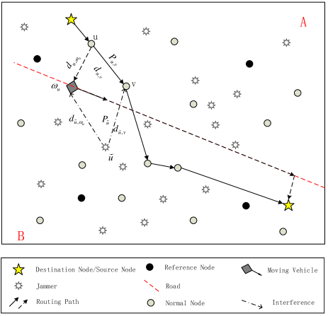
Figure 1: Network topology.

Assume that the locations of the nodes follow a Poisson point process with density $\lambda_{1}$, and the locations of the jammers are governed by another independent Poisson point process with density $\lambda_{2}$. Denoted by $\boldsymbol{\omega}$, the location of a moving vehicle with coordinate $\left(\omega_{x},\omega_{y}\right)$ in the plane $\mathbb{R}^{2}$, and based on the above assumptions, the tuple $\left(\omega_{x},\omega_{y}\right)$ satisfies $a\omega_{x}+\omega_{y}+b=0$ which represents the straight road. In addition, when a moving vehicle is transmitting (or receiving) information to (or from) normal nodes, its location $\boldsymbol{\omega}$ is assumed to be quasi-static as the information transmitted is of a finite size. The road divides the plane into two parts. The source node and destination node are on the either side of the road, respectively. We use plane A to denote the side of the road which the source node is on, and call another side plane B (show as Fig. 1).

Let $\Omega_{A}$ and $\Omega_{B}$ be the sets of nodes in planes A and B respectively, of which the cardinalities are $N_{A}$ and $N_{B}$, respectively. Let $N=N_{A}+N_{B}$. $\Omega^{\prime}$ represents the set of point on the road with a cardinality of $N^{\prime}$. $\Pi$ is the set of all possible links between two normal nodes or between a normal node and the moving vehicle, whose cardinality is $N_{\Pi}$. Let $\varOmega=\Omega_{A}+\Omega_{B}+\Omega^{\prime}$. Then we use $G=(\Omega,\Pi)$ to denote the graph of the network. $\Im$ is the set of jammers. Assume $u,v\in\varOmega$ and $\widetilde{u}\in\Im$ is a jammer. Then the average outage probability from $u$ to $v$ is $P_{u,v}^{\textrm{out}}$. Moreover, we assume that the max node transmit power is $P_{\max}$. However, there is no power constraint for the moving vehicle.

II-B Problem formulation

Frequency non-selective Rayleigh fading is assumed between any pair of trans-receivers, including the nodes, moving vehicles and jammers. The received signal of the link from node $u$ to node $v$ is given as follows

$${y^{(v)}}=\frac{{{h_{u,v}}\sqrt{{P_{u,v}}}}}{{d_{u,v}^{\alpha/2}}}{x^{(u)}}+\sum\limits_{\tilde{u}\in\Im}{\frac{{{h_{\tilde{u},v}}\sqrt{{P_{\tilde{u}}}}}}{{d_{\tilde{u},v}^{\alpha/2}}}{x^{(\tilde{u})}}}+n^{(v)},$$ (1)

where $d_{u,v}$ and $d_{\tilde{u},v}$ are the distance between nodes $u$ and $v$ and the distance between the receiver nodes $v$ and $\widetilde{u}$, respectively. $x^{(u)}$ and $x^{(\widetilde{u})}$ are the transmission signal from the node $u$ and jammer $\widetilde{u}$ , respectively. $P_{u,v}$ and $P_{\tilde{u}}$ are the transmit power of $u$ and $\tilde{u}$, respectively. $h_{u,v}$ and $h_{\tilde{u},v}$ denote the channel fading from node $u$ to node $v$, and the fading between jammer ${\tilde{u}}$ and node $v$, respectively. $\alpha$ refers to the path loss exponent, while $n^{(v)}$ indicates the noise at receiver $v$.

Without loss of generality, we assume that $E[{\left|h_{u,v}\right|^{2}}]=1,\forall u,v\in\Omega+\Omega^{\prime}$ and $E[{\left|{h_{\tilde{u},v}}\right|^{2}}]=1,\forall\tilde{u}\in\Im,v\in\Omega+\Omega^{\prime}$. In our model, because the focus of this research is on the impact of interference on the receive signal, the noise power is ignored. Based on the aforementioned system model, for downlink transmissions, the SIR at the receiver node $v$ from the node u can be written by

$$\textrm{SIR}_{u,v}=\frac{{{P_{u,v}}{\left|h_{u,v}\right|^{2}}d_{u,v}^{-\alpha}}}{{\sum\limits_{\tilde{u}\in\Im}{{P_{\tilde{u}}}{\left|{h_{\tilde{u},v}}\right|^{2}}d_{\tilde{u},v}^{-\alpha}}}}.$$ (2)

To warrant the quality of service (QoS) of the network, the minimum required throughput is assumed to be $\rho$. According to Shannon theory, the threshold of the outage probability is given by

$$\gamma=2^{\rho}-1.$$ (3)

Then outage probability with threshold $\gamma$ in our work is derived as

$$p_{u,v}^{{\rm{out}}} =\Pr\left\{\frac{{{P_{u,v}}{\left|h_{u,v}\right|^{2}}d_{u,v}^{-\alpha}}}{{\sum\limits_{\tilde{u}\in\Im}{{P_{\tilde{u}}}{\left|{h_{\tilde{u},v}}\right|^{2}}d_{\tilde{u},v}^{-\alpha}}}}<\gamma\right\}$$

$$={E_{{h_{\tilde{u},v}}}}\left(1-\exp\left(\frac{{-\gamma\sum\limits_{\tilde{u}\in\Im}{P_{k}}{\left|{h_{\tilde{u},v}}\right|^{2}}d_{\tilde{u},v}^{-\alpha}}}{{{P_{u,v}}d_{u,v}^{-\alpha}}}\right)\right)$$

$$=1-\frac{1}{{\mathop{\prod}\limits_{k\in\Im}\left(1+\frac{{\gamma{P_{k}}d_{\tilde{u},v}^{-\alpha}}}{{{P_{u,v}}d_{u,v}^{-\alpha}}}\right)}}.$$ (4)

Assuming that the length of the information transmitted from $S$ to $D$ is $L$ bits, and as the transmit power and receive power remain constant during transmission, the total consumed energy from node $u$ to node $v$ is shown as

$$E_{u,v}^{\textrm{total}}=\frac{LP_{u,v}}{\rho}.$$ (5)

Attributable to the independence between the hops, the outage probability from node $S$ to $D$ is given as follows

$$p_{S-D}^{{\rm{\textrm{out}}}}=1-\mathop{\prod}\limits_{{l_{u,v}}\in{\Lambda_{S-D}}}(1-p_{u,v}^{{\rm{\textrm{out}}}}),$$ (6)

where $l_{u,v}$ denotes the path from node $u$ to node $v$, $\Lambda_{S-D}$ refers to the set of paths from $S$ to $D$.

Substituting (4) into (6), we arrive at the following outage probability from $S$ to $D$

$$p_{S-D}^{\textrm{out}}=1-\mathop{\prod}\limits_{{\ell_{u,v}}\in{\Lambda_{S-D}}}\frac{1}{{\mathop{\prod}\limits_{\tilde{u}\in\Im}\left(1+\frac{{\gamma{P_{\tilde{u}}}d_{\tilde{u},v}^{-\alpha}}}{{{P_{u,v}}d_{u,v}^{-\alpha}}}\right)}}.$$ (7)

As the nodes in the network are usually power-limited, the essential issue is to minimize the energy consumption from $S$ to $D$, while guaranteeing the QoS. In this context, we formulate the problem with respect to the optimal routing path as follows

$$\Lambda_{\textrm{optimal}}=\underset{\Lambda\in\Lambda_{S-D}}{\arg\min}\left(E_{S-D}\left(\Lambda\right)\right),$$ (8)

where $\Lambda_{\textrm{optimal}}$ denotes the optimal routing path through which the energy consumption of the transmission from $S$ to $D$ is minimized, and the end-to-end outage constraint denoted by $T$ can also be satisfied. Then we can obtain the energy consumption $E_{S-D}$ from $S$ to $D$ as follows

$${E_{S-D}}(\Lambda) =\mathop{\min}\limits_{{P_{u,v}}}\left(\sum\limits_{{l_{u,v}}\in{\Lambda_{S-D}}}{\frac{{{P_{u,v}}L}}{\rho}}\right)$$

$$\textrm{s.t. }p_{S-D}^{\textrm{out}}\leq T,0\leq{P_{u,v}}\leq{P_{\max}},u,v\in\Omega.$$ (9)

Then, the objective function can be derived as

$$\Lambda_{\textrm{optimal}} =\mathop{\arg\min}\limits_{{\Lambda_{S-D}}}\left(\sum\limits_{{l_{u,v}}\in{\Lambda_{S-D}}}{\frac{{{P_{u,v}}L}}{\rho}}\right)$$

$$\textrm{s.t. }1-\mathop{\prod}\limits_{{\ell_{u,v}}\in{\Lambda_{S-D}}}\frac{1}{\prod\limits_{\tilde{u}\in\Im}\left(1+\frac{{\gamma{P_{\tilde{u}}}d_{\tilde{u},v}^{-\alpha}}}{{{P_{u,v}}d_{u,v}^{-\alpha}}}\right)}\leq T,$$

$$\qquad u,v\in\Omega,0\leq{P_{u,v}}\leq{P_{\max}}.$$ (10)

Similar to the situation in which we need to find the routing path when the end-to-end delay is bounded [14], the problem in this paper cannot be solved by traditional shortest path algorithms such as the Dijkstra and Bell-Ford algorithms. There are some ways to tackle this problem. The first one is to enumerate all possible solutions and then to identify the best routing path that minimizes energy consumption. However, in this problem, the transmission power is continuous. That is so-called NP-complete problem. So, we cannot find the best solution in this way. Secondly, the authors in [12] proposed an algorithm termed the Minimum Energy Routing With Approximate Outage Per Link (MER-AP) algorithm, which applies the Lagrange multipliers technique to assign each link power a certain expression formula. But in this paper , the transmission power is bounded, while the transmission power in [12] is a function of the distance of each link, the path loss exponent as well as the interference of jammers, which may surpass the constraint of the max transmission power. As a result, MER-AP is not suitable for this paper’s problem. The last one is to obtain an approximate expression and use the Dijkstra algorithm or other methods to derive a sub-optimal solution.

III Optimal Routing Path Algorithm

In this section, we propose a three-step algorithm to find the optimal routing path such that the total energy consumption is minimized, while guaranteeing the end-to-end outage constraint. Before detailing our proposed algorithm, some related assumptions should be addressed first.

Assumption 1: In this paper, we assume the total energy consumption of the network does not include the vehicle’s energy consumption. This is because the moving vehicle is not considered as part of the network, so its energy consumption will not be taken into account in the objective function.

Assumption 2: The vehicle just communicates with its closest node in plane B.

Assuming the fixed node $u$ communicates with the moving vehicle, the average outage probability can be obtained as follows

$$p_{u,\omega_{u}}^{\textrm{out}}=1-\frac{1}{{\mathop{\prod}\limits_{\tilde{u}\in\Im}\left(1+\frac{{\gamma{P_{\tilde{u}}}d_{\tilde{u},v}^{-\alpha}}}{{{P_{u,{\omega_{u}}}}d_{u,{\omega_{u}}}^{-\alpha}}}\right)}},$$ (11)

where $\omega_{u}$ is the point where the fixed node $u$ communicates with the moving vehicle, and $\omega_{u}\in\varOmega^{\prime}$. If proper routing is ensured, the moving vehicle can act as a relay in the network to transmit information. In addition, the moving vehicle can also carry information over a long distance before transmitting it to the fixed nodes in plane B. The total energy can be saved to a great extent. However, to meet the end-to-end outage constraint as well as making our considered scenario more practical, the locations where the vehicle receives information from the fixed node $u$ in plane A should be selected wisely, which should satisfy the following

$$(\omega_{x}^{\prime},\omega_{y}^{\prime})=\arg\max\limits_{\omega_{u}}\left(p_{u,\omega_{u}}^{\textrm{out}}\right).$$ (12)

As the energy consumed by the moving vehicle is not considered, the optimal routing path is actually divided into two sub-paths, i.e., from $S$ to the moving vehicle and from the moving vehicle to $D$. Intuitively, the two sub-paths can be obtained in two separate planes, i.e., planes A and B, as illustrated in Fig. 1. To reduce the complexity of identifying the optimal routing path, we assume that each hop along the routing path has an equal outage constraint, i.e.,

$$p_{u,v}^{{\rm{\textrm{out}}}}(m)=1-\sqrt[m]{{1-T}},st.{l_{u,v}}\in{\Lambda_{S-D}},$$ (13)

where $m$ is the number of hops. As can be seen from (13), the transmit power of each hop $p_{u,v}^{{\rm{out}}}(m)$ is highly related to the number of hops, which is unknown in our model. Conditioned on $m$, the optimal sub-path in plane A which is denoted as $\Lambda_{optimal}^{A}(n)$ with a $n$-hop (n=1,2…,m-1) path, and the optimal sub-path in plane B denoted as $\Lambda_{optimal}^{B}(m-n)$ can be found using our proposed algorithm, in which the number of hops in plane B is $m-n$. After searching all possible $m$, the optimal routing path then is attainable. Based on the above analysis, we propose a three-step dynamic programming based algorithm to find the optimal routing path.

III-A Routing Algorithm in Plane A

Algorithm 1 Dynamic Programming Routing Selection on Plane A

1: for all $u,v\in{\Omega_{A}},{P_{S,u}}\leqslant{P_{\max}}$do

2:   ${C_{S-u}}(1)\left|{{}_{{\Pi_{S-u}}}}\right.={P_{S,u}}\cdot L/\rho$

3: end for

4: for all $u,v,u^{\prime}\in{\Omega_{A}},{P_{u,v}}\leqslant{P_{\max}}$ do

5:   for i=2 to n-1 do

6:     $u^{\prime}=\mathop{\arg\min}\limits_{u}({C_{S-u}}(i-1)+{P_{u,v}}\cdot L/\rho)$

7:     ${C_{S-v}}(i)={C_{S-u^{\prime}}}(i-1)+{P_{u^{\prime},v}}\cdot L/\rho$

8:     ${\varPi_{S-v}}(i)$=${\varPi_{S-u^{\prime}}}(i-1)+l_{u^{\prime},v}$

9:   end for

10: end for

11: for all $u,\in{\Omega_{A}},{P_{u,{\omega^{\prime}_{u}}}}\leqslant{P_{\max}}$do

12:  ${C_{S-{\omega^{\prime}_{u}}}}(n)={C_{S-u}}(n-1)+{P_{u,{\omega_{u}}}^{\min}}\cdot L/\rho$

13:  ${\varPi_{S-{\omega^{\prime}_{u}}}}(n)$=${\varPi_{S-u}}(n-1)+l_{u,{\omega^{\prime}_{u}}}$

14: end for

15: return $\Lambda_{optimal}^{A}(n)=\mathop{\arg\min}\limits_{{\Pi_{S-{\omega^{\prime}_{u}}}}(n)}({C_{S-{\omega^{\prime}_{u}}}}(n))$=${\varPi_{S-{\omega^{\prime}_{u}}}}(n)$

In plane A, we should choose the optimal routing path from $S$ to the moving vehicle. We maintain minimum energy consumption of the h-hop link path from $S$ to node $u$, denoted as ${\Pi_{S-u}}({\text{h}})$, of which the corresponding minimum cost is ${C_{S-u}}$(h). Firstly, when hop=1 and for each node $u$ in plane A, we can derive ${C_{S-u}}(1)={\raise 3.01385pt\hbox{${{P_{S,u}}\cdot L}$}\!\mathord{\left/{\vphantom{{{P_{S,u}}\cdot L}\rho}}\right.\kern-1.2pt}\!\lower 3.01385pt\hbox{$\rho$}}$, where $P_{S,u}\leq P_{max}$. Then, when hop is $h\>(h=2,3\ldots,n-1)$, for each node $u$ and node $v$ in plane A, the minimum energy consumption is shown as

$${C_{S-u}}(h)=\min(P_{v,u}\cdot L/\rho+{C_{S-v}}(h-1)).$$ (14)

And then we can refresh the h-hop path according to

$${\Pi_{S-u}}(h)={\Pi_{S-t}}(h-1)+{l_{t,u}},$$ (15)

where $t=\mathop{\arg\min}\limits_{v\in\varOmega_{A}}(P_{v,u}\cdot L/\rho+{C_{S-v}}(h-1))$. And we denote the optimal location of the moving vehicle satisfying (13) when node $u$ in plane A communicates with the moving vehicle, which is the last hop in plane A. So we can have the minimum energy of node $u$ communicating with moving vehicle, denoted as $p_{u}^{\textrm{min}}$, which accords with (13). Adding this power to ${C_{S-u}}(n-1)$ of every node $u$ in plane A, we can choose the minimum energy consumption in plane A with the n-hop path ${\varPi_{S-u}}(n)$.

III-B Routing Algorithm on Plane B

Algorithm 2 Dynamic Programming Routing Selection on Plane B

1: for all $\varsigma,v\in{\Omega_{B}},{P_{\varsigma,v}}\leqslant{P_{\max}},\varsigma\in\Theta$ do

/*$\Theta$ is the set of the nodes that is closed to the trace of

moving vehicle

2:   ${C_{\varsigma-v}}(1)\left|{{}_{{\Pi_{\varsigma-v}}(1)}}\right.={{P_{\varsigma,v}}\cdot L/\rho}$

3: end for

4: for all $u,v,u^{\prime}\in{\Omega_{B}},{P_{u,v}}\leqslant{P_{\max}},\varsigma\in\Theta$do

5:   for i=2 to m-n do

6:     $u^{\prime}=\mathop{\arg\min}\limits_{u}({C_{\varsigma-u}}(i-1)+{P_{u,v}}\cdot L/\rho)$

7:     ${C_{\varsigma-v}}(i)={C_{\varsigma-u^{\prime}}}(i-1)+{P_{u^{\prime},v}}\cdot L/\rho$

8:     ${\varPi_{\varsigma-v}}(i)$=${\varPi_{\varsigma-u^{\prime}}}(i-1)+l_{u^{\prime},v}$

9:   end for

10: end for

11: return $\Lambda_{optimal}^{B}(m-n)=\mathop{\arg\min}\limits_{{\Pi_{\varsigma-D}}(n),\varsigma\in\Theta}({C_{\varsigma-D}}(m-n))$=${\varPi_{\varsigma-v}}(m-n)$

In plane B, as we ignore the energy consumption of the link between the moving vehicle and the fixed nodes in plane B, there is still a $(m-n)$-hop path in plane B. We firstly obtain the closest node set denoted as $\Theta$ to the moving vehicle when the moving vehicle transmits information to the fixed nodes in plane B. Then we can get $min(C_{u-D}(m-n)),u\in\Theta$ using a similar algorithm in SectionIII-A to get the minimum energy consumption with the $(m-n)$-hop routing path ${\Pi_{u-D}}(m-n),u\in\Theta$.

III-C Optimal Routing Path

Algorithm 3 Find the Optimal Path

1: for m=2 to N-1 do

2:   for n=1 to m-1 do

3:     using Algorithm1 to get the $\Lambda_{optimal}^{A}(n)$

4:     using Algorithm2 to get the $\Lambda_{optimal}^{B}(m-n)$

5:   end for

6: end for

7: return ${\Lambda_{optimal}}$

We calculate the transmit power of each link according to (13), when $m$ varies from 2 to $N$-1 for each plane with an one-hop path at least considering the algorithm with the moving vehicle involved. Then the number of hops in plane A changes from 1 to $m-1$, corresponding to the number of hops in plane B changes from $m-1$ to 1. Then we can add up the minimum energy consumption of the entire network. And the optimal routing path can derived as ${\Lambda_{optimal}}={\varPi_{S-{\omega^{\prime}_{u}}}}(n)+{\Pi_{u-D}}(m-n)+l_{{\omega^{\prime}_{u}},u},u\in\Theta,n=1,...,m-1,m=1,...,N-1$.

III-D Discussion

The algorithm described above only considers the optimal routing selection considering that the moving vehicle must involve information transmission. This is to say, the moving vehicle satisfies all the possible positions in order to transmit information. In a practical scenario, the reference node will take the motion trajectory of the moving vehicle into account. Moreover, the locations of the source node and the destination node are also needed to be taken into consideration when deciding whether or not the moving vehicle should participate in information exchange.

In this paper, because we keep the value of the minimum energy and the corresponding $m$-hop path selection for each operation, the computational complexity of the algorithm is $O(N^{4})$ regardless of the involvement of the moving vehicle. However, for the method proposed in [15], which also considers the participation of the moving vehicle, the complexity of its algorithm will be increased to $O(N^{4}logN)$. Therefore, the algorithm complexity proposed in this paper is lower than that of the MER-EQ algorithm in [15] for the scenarios under consideration.

IV Results and Discussions

Without loss of generality, we assume that the closest system node to point $(0,0)$ is source $S$, while the closest system node to point $(100,100)$ is the destination $D$. A snapshot of the network with an area of $100m\times 100m$ is illustrated in Fig. 2, where $\lambda_{1}=0.43$, the corresponding number $N=47$, $\lambda_{2}=0.15$, the corresponding number of jammers is 17, the equation of road is $3x+10y-700=0$, $P_{\widetilde{u}}=0.1\textrm{W}$, $\alpha=2$, $P_{\textrm{max}}=15\textrm{W}$ , $T=0.1$, and $L/\rho=1\textrm{s}$ [16].

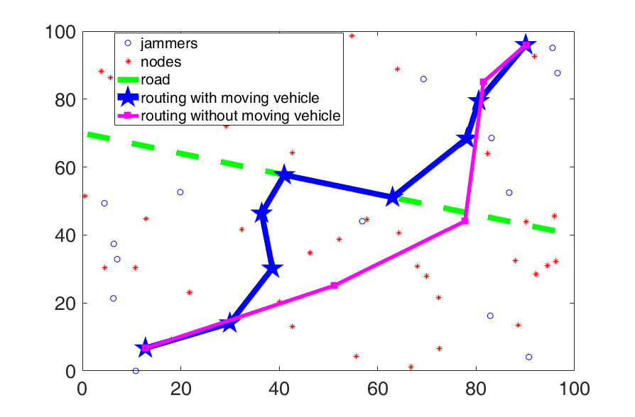
Figure 2: Optimal routing path with and without moving vehicles when $\alpha=2$.

In Fig. 2, the blue line indicates the selected optimal path involving moving vehicles, while the pink line is the selected optimal routing path without the moving vehicles when $\alpha=2$. Besides, it is found that the minimum energy consumption of the blue line is about 60% of the pink one, showing that the routing path involving the moving vehicles can save much energy compared with the scenario without the vehicle. What’s more, the number of hops needed in the routing path with moving vehicles is more than that without moving vehicles, e.g., 8 hops versus 4 hops in Fig. 2, indicating that the average energy consumption per node is lower and thus beneficial in terms of prolonging the service time of the networks.

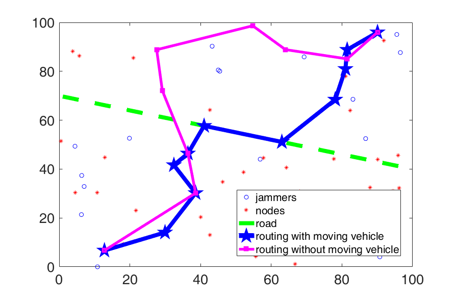
Figure 3: Optimal routing path with and without moving vehicles when $\alpha=3$.

The optimal routing paths with and without the moving vehicles when $\alpha=3$ are illustrated in Fig. 3. Compared with Fig. 2, the optimal routing path is totally different. Besides, by utilizing moving vehicles, the total energy consumption can be saved up to 75%, which indicates that the path loss exponent has a great impact on routing path selection and energy consumption. To further reveal the reason behind, Fig. 4 plots the energy consumption as a function of the end-to-end outage probability threshold with different path loss exponents.

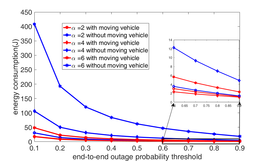
Figure 4: Total energy consumption vs. the end-to-end outage probability threshold $T$.

Without the maximum transmit power constraint, the total energy consumption versus the end-to-end outage probability threshold $T$ with different path loss exponents $\alpha$ is depicted in Fig. 4. It is shown that the energy consumption of the network decreases with the increase of the end-to-end outage probability threshold, thanks to a higher requirement of QoS for communications. As for relationship between the path loss exponents and transmit power of each link, we can obtain $p_{u,v}^{\textrm{out}}\approx 1-\exp\left(-\frac{{d_{u,v}}^{\alpha}\cdot\gamma}{P_{u,v}}\cdot\sum\limits_{\widetilde{u}}{{P_{\widetilde{u}}}d_{\widetilde{u},v}^{-\alpha}}\right)$ from the fact that $e^{x}\geq 1+x$ for $x\geq 0$. And then we can obtain $P_{u,v}(\alpha)\propto{d_{u,v}}^{\alpha}\cdot\gamma\cdot\sum\limits_{\widetilde{u}}{{P_{\widetilde{u}}}d_{\widetilde{u},v}^{-\alpha}}=\gamma\cdot{\sum\limits_{\widetilde{u}}{{P_{\widetilde{u}}}(\frac{{d_{u,v}}}{{d_{\widetilde{u},v}}})}^{\alpha}}$ based on (13). $\frac{{d_{u,v}}}{{d_{\widetilde{u},v}}}$ has a different effect on the transmit power $P_{u,v}$. For instance, when $\frac{{d_{u,v}}}{{d_{\widetilde{u},v}}}>1$ , the transmit power increases with the path loss exponents, and decreases the other way round. Thus, we can find that the sum energy consumption when $P_{u,v}$ is higher than when $\alpha=4$, but lower than when $\alpha=6$. The same can be concluded from Figs. 2 and 3. The minimum energy consumption involving the moving vehicle in Fig. 3 is lower than that in Fig. 2.

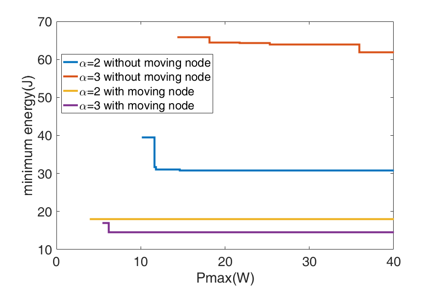
Figure 5: Minimum energy consumption vs. the maximum power constrain.

Fig. 5 shows the minimum network energy consumption as a function of the maximum power constrain $P_{\max}$ with different path loss exponents when $T=0.1$. It is found that the minimum network energy consumption decreases with the increase of $P_{\max}$, indicating that a strict QoS constraint, i.e., the configuration of $T$, makes it more difficult to transmit information in a small number of hops, and thus the system requires a greater number of hops when $P_{\max}$ is low. Moreover, when $P_{\max}$ exceeds a certain value, the minimum network energy consumption remains constant. By contrast, there is no proper routing path between $S$ and $D$, when $P_{\max}$ is lower than a given value denoted by $\overline{P_{\max}}$. It is also noted that the value of $\overline{P_{\max}}$ is smaller when transferring information with the moving vehicles than without the moving vehicle.

V Conclusions and Future Work

In this paper, we investigated the optimal routing path design in suburban areas by jointly considering the per-node maximum transmit power constraint, QoS and energy-efficient communications. In our model, moving vehicles are used to assist in information transportation. A three-step algorithm was proposed to find the optimal routing path with a computational complexity of $O(N^{4})$. Besides, results were presented to show that with the assistance of a moving vehicle, the total energy consumed can be reduced greatly. We also studied the impact on routing path design and energy consumed caused by the path loss exponent, maximum transmit power constrain and QoS requirement. In our future work, a multi-point-topoint transmission method will be considered.

References

- [1] Ericsson, Ericsson White Paper, January 2016, available at: https://www.ericsson.com/assets/local/publications/white-papers/wp_iot.pdf.
- [2] W. Xiang, K. Zheng, and X. Shen, 5G Mobile Communications. Springer, 2016.
- [3] Ericsson, Ericsson Mobility Report, November 2015, available at: http://www.ericsson.com/res/docs/2015/mobility-report/ericsson-mobility-report-nov-2015.pdf.
- [4] M. T. Rahama, M. Hossen, and M. M. Rahman, “A routing protocol for improving energy efficiency in wireless sensor networks,” in Proc. ICEEICT, pp. 1–6.
- [5] T. T. Huynh, A. V. Dinh-Duc, and C. H. Tran, “Delay-constrained energy-efficient cluster-based multi-hop routing in wireless sensor networks,” Journal of Communications and Networks, vol. 18, no. 4, pp. 580–588, Sep. 2016.
- [6] D. H. Tran and D. S. Kim, “Minimum latency and energy efficiency routing with lossy link awareness in wireless sensor networks,” in 2012 9th IEEE International Workshop on Factory Communication Systems, pp. 75–78.
- [7] N. Jan, N. Javaid, Q. Javaid, N. A. Alrajeh, M. Alam, Z. A. Khan, and I. A. Niaz, “A balanced energy consuming and hole alleviating algorithm for wireless sensor networks,” IEEE Access, vol. PP, no. 99, pp. 1–1, 2017.
- [8] A. Bazzi, B. M. Masini, A. Zanella, and G. Pasolini, “Vehicle-to-vehicle and vehicle-to-roadside multi-hop communications for vehicular sensor networks: Simulations and field trial,” in Proc. ICC, 2013, pp. 515–520.
- [9] G. Korkmaz, E. Ekici, and F. Ozguner, “An efficient fully ad-hoc multi-hop broadcast protocol for inter-vehicular communication systems,” in Proc. ICC, vol. 1, 2006, pp. 423–428.
- [10] O. Tonguz, N. Wisitpongphan, F. Bait, P. Mudaliget, and V. Sadekart, “Broadcasting in vanet,” in 2007 Mobile Networking for Vehicular Environments, pp. 7–12.
- [11] X. Ge, H. Cheng, G. Mao, Y. Yang, and S. Tu, “Vehicular communications for 5g cooperative small-cell networks,” IEEE Transactions on Vehicular Technology, vol. 65, no. 10, pp. 7882–7894, Apr., 2016.
- [12] A. Sheikholeslami, M. Ghaderi, H. Pishro-Nik, and D. Goeckel, “Jamming-aware minimum energy routing in wireless networks,” in Proc. ICC, 2014, pp. 2313–2318.
- [13] M. Zhao, I. W. H. Ho, and P. H. J. Chong, “An energy-efficient region-based rpl routing protocol for low-power and lossy networks,” IEEE Internet of Things Journal, vol. 3, no. 6, pp. 1319–1333, Jul., 2016.
- [14] W. Zheng and J. Crowcroft, “Quality-of-service routing for supporting multimedia applications,” IEEE Journal on Selected Areas in Communications, vol. 14, no. 7, pp. 1228–1234, Aug. 1996.
- [15] A. Sheikholeslami, M. Ghaderi, H. Pishro-Nik, and D. Goeckel, “Energy-efficient routing in wireless networks in the presence of jamming,” IEEE Transactions on Wireless Communications, vol. 15, no. 10, pp. 6828–6842, Oct. 2016.
- [16] X. Ge, S. Tu, T. Han, Q. Li, and G. Mao, “Energy efficiency of small cell backhaul networks based on gauss-markov mobile models,” IET Networks, vol. 4, no. 2, pp. 158–167, Mar., 2015.