Ultra Compact Stars: Reconstructing the Perturbation Potential
Abstract
In this work we demonstrate how different semi-classical methods can be combined in a novel way to reconstruct the perturbation potential of ultra compact stars. Besides rather general assumptions, the only specific information entering this approach is the spectrum of the trapped axial quasi-normal modes. In general it is not possible to find a unique solution for the potential in the inverse problem, but instead a family of potentials producing the same spectrum. Nevertheless, this already determines important properties of the involved potential and can be used to rule out many candidate models. A unique solution was found based on the additional natural assumption that the exterior part () is described by the Regge-Wheeler potential. This is true in general relativity for any non-rotating spherically symmetric object. This technique can be potentially applied for the study of deviations from general relativity. The methods we demonstrate are easy to implement and rather general, therefore we expect them also to be interesting for other fields where inverse spectrum problems are studied, e.g. quantum physics and molecular spectroscopy.
pacs:
04.40.Dg, 04.30.-w , 04.25.Nx, 03.65.GeI Introduction
With the repeated detection of gravitational waves from presumably binary black hole mergers by LIGO Abbott et al. (2016, 2016, 2017) and its confirmation of different predictions of general relativity Abbott et al. (2016), it might seems clear that black holes exist in nature and exotic alternatives are more unlikely to exist. However, recent claims of discovered “echoes” in LIGO data Abedi et al. (2016, 2017) show that there could be room for different kind of alternative black hole models or observable quantum gravitational effects Cardoso et al. (2016a, b); Barceló et al. (2017); Nakano et al. (2017); Holdom and Ren (2017); Novotný et al. (2017); Stuchlík et al. (2017). Although technical parts of the signal analysis have been criticized Ashton et al. (2016), a full treatment of the problem and more observations have to be carried out for clarification.
The gravitational wave signature of many alternative ultra compact objects is expected be in agreement with the observed signal during the inspiral phase and interestingly also, at the later phases, for the part of the signal that corresponds to the first ringdown mode. In contrary to black holes, it is predicted that additional structure in the signal shows up at later times, recently often called “echoes” Ashton et al. (2016); Damour and Solodukhin (2007); Cardoso et al. (2016a, b); Konoplya and Zhidenko (2016a); Price and Khanna (2017); Brustein et al. (2017); Nakano et al. (2017), which might be associated with the excitation of trapped modes of the object Chandrasekhar and Ferrari (1991); Kokkotas (1994); Kojima et al. (1995); Kokkotas (1995); Andersson et al. (1996); Tominaga et al. (1999); Kokkotas and Schmidt (1999); Benhar et al. (1999); Ferrari and Kokkotas (2000). Thus, up to now, it is not possible to rule out such alternative objects based on the available gravitational wave observations and it remains an open problem Konoplya and Zhidenko (2016b); Ashton et al. (2016). For an extended and recent overview about echoes and alternative objects we refer to Cardoso and Pani (2017).
In the case that future detections contain additional structure in the signal, one would obviously be interested in the nature of the object. The conventional way to tackle such a problem is to build a model for the object and check if the predicted signal agrees with observation. This is reasonable and straight forward, but has the drawback that one is limited to the models available and laboriously has to solve the direct problem many times to hopefully fit the observation. In this article, we propose an alternative approach which can be used to study the problem the inverse way.
The inverse problem uses the observable data to recover the properties of the source. More specifically, in this work we show how the trapped axial mode spectrum of the source can be used to reconstruct the potential producing the spectrum. Using future gravitational wave observations it should be possible to determine the spectrum from the waveform if the unique features (“echoes” or “trapped” modes) characterizing the specific object are excited following the dominant black-hole-type quasi-normal mode.
It is known that to linear order axial perturbations of spherically symmetric and non-rotating objects reduce to a one-dimensional wave equation for the radial part of the perturbation, called Kokkotas and Schmidt (1999); Nollert (1999); Berti et al. (2009); Konoplya and Zhidenko (2011)
| (1) |
where are the quasi-normal modes and an effective potential. The direct problem in this case is to calculate from . The inverse problem is to use the information provided by a known/observed spectrum in order to re-construct the associated potential . In general, one does not expect to find a unique answer to this problem, but based on rather general and reasonable assumptions, it is possible to simplify the problem significantly and obtain a unique solution in many cases. Here we demonstrate that for ultra compact stars there is a way to extract a unique solution for the potential.
This paper is organized as follows. In section II we present the mathematical details of our approach for solving the inverse problem. In section III we demonstrate how the method can be applied to constant density stars and gravastars. We discuss our findings in section IV while section V contains our conclusions. We provide more details about our implementation and additional results in the Appendix (section VI).
Throughout the paper, we assume .
II The Inverse Problem
Inverse problems arise in various fields of science and engineering and are usually much harder to solve than their direct counterpart. Inverse problems can be ill posed and even for simple problems it might be impossible to find a unique solution. An overview about the inverse problem in the context of this work can be found in Wheeler (2015); Chadan and Sabatier (1989); Lazenby and Griffiths (1980); Gandhi and Efthimiou (2006). A classical example for the inverse problem is the question whether one can hear the shape of a drum Kac (1966); Gordon et al. (1992). It turns out that the same spectrum of eigenvalues can be produced by different shapes, what means that the inverse problem in this case is not unique.
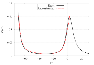
We are interested in the inverse problem for the one-dimensional wave equation (1) with a typical effective potential for many ultra compact horizonless objects. The qualitative shape of such a potential can be described by the combination of a bound region next to a potential barrier and is shown in figure 1. The barrier at of the potential corresponds to the photosphere and is the same for black holes and ultra compact stars. The surface of ultra compact stars is somewhere between the potential barrier and the diverging part of the potential, which corresponds to the center of the star. For black holes there is no internal barrier and the potential asymptotically tends to zero. This difference in the potentials of the two systems, leads to a completely different quasi-normal mode spectrum. In Völkel and Kokkotas (2017), hereafter called paper I, we have shown that the widely known Bohr-Sommerfeld methods are useful tools, because they provide a simple framework to obtain useful approximate results and allow for an analytic treatment when considering problems of this kind. Therefore, in this work, we employ such approximate methods and demonstrate how surprisingly precise they can be in solving the inverse problem.
In paper I, we demonstrated that it is possible to treat the direct problem as a combination of a pure bound state and a barrier problem. We adopt the same structure and approach the inverse problem in three steps. First, we calculate the so-called excursion , which is the width of the bound region between the first two turning points . Second, we determine the corresponding width of the barrier between the turning points . In the third step we make the additional assumption that the external potential for is described by the Regge-Wheeler potential Regge and Wheeler (1957). This assumption provides in principle the third turning point , which together with and leads to a unique solution for the potential .
In literature related to the inverse problem, one usually finds and not as definition for the spectrum, thus we adopt this notation. The connection between the trapped quasi-normal modes and the spectrum is given by
| (2) |
where and are the real and imaginary part of . In different steps of the method one needs to inter- and extrapolate the spectrum. We provide details for this rather technical issue in the Appendix (section VI.1).

II.1 Recovering the Bound Region
The solution to the bound state problem is known for a long time Wheeler (2015); Chadan and Sabatier (1989) and consists of several steps. It has already been applied in different fields, e.g. molecular spectroscopy and quantum algebra Bonatsos et al. (1991, 1992a, 1992b).
The first step is to find from . In a potential of the kind shown in figure 1 we expect a finite number of states and a discrete function for . However, in the method one needs to have a continuous function for , because it involves integration. To make it continuous one can interpolate between all bound states and extrapolate to the minimum of the potential.
Starting then from the now approximatively known one has to calculate the so-called “inclusion” defined as
| (3) |
Here is the minimum of the potential. This information is not directly known from the spectrum, but can be approximated from the point where extrapolates to zero. The inclusion is used as an intermediate function to determine the excursion
| (4) |
which is the width of the bound potential for a given energy and are the classical turning points. Without further assumptions there are infinitely many WKB equivalent potentials satisfying the above relation and producing the same spectrum. To get a unique solution one has to provide or for one side of the potential. The knowledge of its width then determines the other side. We will use a natural assumption once the barrier region is recovered. Nevertheless, even the knowledge of can easily be used to rule out different models, because their corresponding will in general not agree with the reconstructed one.
II.2 Recovering the Barrier Region
The semi-classical reconstruction of a one-dimensional potential barrier from the so-called transmission is known in the literature Lazenby and Griffiths (1980); Gandhi and Efthimiou (2006) and we will use the method provided in Gandhi and Efthimiou (2006). In our case it will only be possible to determine the width of the barrier for a given energy
| (5) |
here are the classical turning points for the potential barrier and the maximum of the potential. is not known from the spectrum but can be extrapolated. is the transmission and in semi-classical approximation given by
| (6) |
To reconstruct the potential one needs to know the continuous function , but since we want to limit our knowledge to the trapped quasi-normal modes we only have discrete values for . Can the transmission be determined from the spectrum ? In our case it is approximatively possible by using that the potential to the left of the barrier is described by a bound region shown in figure 1. Within the Bohr-Sommerfeld framework one can show that the imaginary part of the spectrum for can be approximated with
| (7) |
which contains explicitly the expression for the transmission (6) evaluated for , see paper I. The approximation is justified because the imaginary part of trapped modes is typically many orders of magnitude smaller than their real part (). The transmission can now be approximated with
| (8) |
Note that due to the discreteness of , one only can calculate only discrete values of the transmission. The integral in equation (8) contains the part of the bound region potential between and , which is not known. Fortunately, it can be proven that the integral is equivalent for any potential within the family already known from the reconstruction of , the proof is provided in Appendix (section VI.2). For simplicity and without loss of generality, one can use the symmetric potential with the turning points for integration. The width of the barrier is then approximatively known after inserting the interpolated transmission into equation (5).
II.3 A Unique Solution
Without further assumptions one can not find a unique solution for . The reconstructed widths and are however very powerful results which can be used to test if a specific model, for any choice of its parameters, can reproduce them. It is trivial to calculate the widths of the bound region and the potential barrier for any given model. This allows to exclude models if the widths differ from the reconstructed ones, but importantly does not prove that the model is correct. There are infinitely many potentials which can be “tilted” or “shifted”, but have the same widths and . This non-uniqueness disappears if one of the three turning points of the potential is provided.
In general relativity, there is one “natural” assumption for non-rotating spherically symmetric objects, that is the Birkhoff’s theorem Birkhoff (1923). It states that the external spacetime is described by the Schwarzschild solution. As a result the Regge-Wheeler (RW) potential will uniquely describe the axial perturbations of the exterior spacetime. Thus for the region on right of the potential barrier i.e. for we will use the RW potential, defining in a unique way the third turning point . It follows that the other two turning points are then given by
| (9) |
Finally, the inversion of and with respect to determines the unique solution for the reconstructed interior part of the potential . Here and correspond to the minimum in the bound region and maximum of the potential barrier, respectively.
There is however one case where we can not use the previously explained assumption to find a unique solution. If the potential in the bound region becomes negative, there is no third corresponding turning point and therefore no unique solution. However, the potential for typical systems like constant density stars and gravastars is positive everywhere, while a negative region would be the signal of instabilities. Therefore we exclude such cases in the present work. Still, even unstable cases could be studied by using the same method.
Obviously, the potential which has been reconstructed with approximative methods cannot be exact. There are two different kind of approximations involved. The first one is the general use of semi-classical methods and the second one the specific details of the inter- and extrapolation from the finite number of known states. Only if both kind of approximations are valid one can expect precise results.
III Application and Results
In this section we apply the previously demonstrated methods to two different types of ultra compact objects. Constant density stars are the typical type of objects for any study of this kind, because they are simple to treat analytically and numerically. Their oscillations have intensively been studied in Chandrasekhar and Ferrari (1991); Kokkotas (1994); Kojima et al. (1995); Andersson et al. (1996); Kokkotas (1995); Tominaga et al. (1999); Ferrari and Kokkotas (2000) and in paper I. A second type of ultra compact objects are the more exotic gravastars Mazur and Mottola (2001). The values of the trapped mode frequencies used here, have been derived by a full numerical code discussed in Kokkotas (1994) and are tabulated in the Appendix (section VI.4).
The linear perturbations of both systems, in the non-rotating case, can effectively be described by the one-dimensional wave equation
| (10) |
where is the radial part of the metric perturbation. The wave equation appears in the so-called tortoise coordinate , which is a function of the normal Schwarzschild coordinate . Its explicit form has to be calculated for every system specifically. For more details we refer to Kokkotas and Schmidt (1999).
In this work we limit ourselves to the non-rotating case because the axial perturbation equations decouple to a one dimensional wave equation, which does not work for rotating systems. For sure rotation will play an important role for realistic systems, but its treatment within the analytic framework presented here is out of scope of this work. It is reasonable to assume that slow rotation studied in Kojima (1992); Kokkotas et al. (2004) will not change the qualitative results. We plan to extend the inverse method also to rotating systems in the future.
III.1 Constant Density Stars
The axial mode potential for constant density stars is given by
| (11) |
where is the harmonic index from the expansion of the metric perturbation in spherical tensor harmonics. and are the density and pressure, respectively. is the integrated mass function from the center of the star to , while the normalization is also used. The potential appearing in the wave equation (10) is expressed in terms of the Schwarzschild coordinate , which is related to the tortoise coordinate , as follows
| (12) |
where and are the and components of the metric tensor . An explicit analytic form can be found in Pavlidou et al. (2000). Constant density stars obey the Buchdahl limit, which sets as limit for the most compact model.
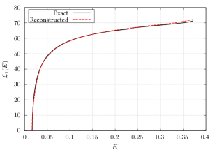
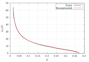
In figures 2 and 3 we present our results for constant density stars with and . More results for can be found in the Appendix (section VI.3). Each figure consists of three panels and is structured from left to right as follows. The left panel shows the relative width of the bound region and the central panel shows the width of the potential barrier . The right panel compares the result for the reconstructed potential with the exact potential. In every panel the black solid curve describes the exact function, while the red dashed curve shows our reconstructed result. In the caption we provide the total number of trapped modes that exist in the specific potential and have been used for the reconstruction.


III.2 Gravastars
In contrast to constant density stars, gravastars refer to a wider class of exotic stars. There are models with different layers, where the interior consists of a de Sitter condensate with . In this work we study the simplified thin shell model, because our primary interest is to show the applicability of our methods to the inverse problem. The thin shell model assumes an infinitely thin shell at radius , which separates the interior and exterior spacetime. For comprehensive work about the physics of gravastars and their perturbations we refer to Mazur and Mottola (2001); Visser and Wiltshire (2004); Chirenti and Rezzolla (2007); Pani et al. (2009, 2010); Cardoso et al. (2014); Chirenti and Rezzolla (2016).
The axial mode potential for thin shell gravastars is given by
| (13) |
Here is again the harmonic index and the density. This model corresponds to the specific equation of state in the shell with zero surface density. The wave equation is written again in terms of the tortoise coordinate , which in the interior region is given by the relation
| (14) |
Here is a constant of integration, chosen by demanding that continuously matched with the usual exterior Schwarzschild tortoise coordinate
| (15) |
where stands for the radius of the gravastar. The models were parametrized with respect to i.e. the compactness.
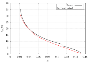
We present results for gravastars with in figure 4 and provide additional results for less compact gravastars with and in the Appendix (section VI.3). We have chosen results for , since the number of trapped modes for is typically small and the deviations between the true and the reconstructed potential can be large. The appearance of unphysical deformations in the reconstructed potentials for small is discussed in section IV.


IV Discussion
Here we discuss the results presented in section III. In general we find that the agreement between exact and recovered widths, both for and , is quite good and significantly improves with the number of existing trapped modes in the potential. This connection is natural since the more modes are available, the more accurate become the interpolations and extrapolations used for deriving the basic ingredients of the method, which are the spectrum and the transmission . Because the method is based on WKB theory and for practical purposes has to use inter- and extrapolation, one can not clearly define a minimum number of necessary trapped modes for a desired accuracy of the final result. Our results provide a good estimate what accuracy can be expected for different numbers of existing trapped modes.
Since the height of the potential barrier increases strongly with rising , also the number of existing trapped modes increases. From this one can conclude that the method becomes more precise for large values of , which corresponds to the eikonal limit.
The width of the barrier seems to be systematically underestimated. This tendency is noticeable if the number of trapped modes is small and becomes less visible otherwise. By studying the direct problem with semi-classical methods in paper I, we found that the imaginary parts of the trapped modes are systematically underestimated for the higher order modes. Thus we make the guess that the systematic deviation is related to the semi-classical methods themselves and does not originate from the details of inter- and extrapolation.
Comparing the results for the two different types of objects we studied, one finds that the results for constant density stars are significantly more precise than for gravastars. We want to make three comments here. First, the number of trapped modes for the specific gravastar models is smaller and the inter- and extrapolation therefore less precise. Second, from the calculation of the trapped modes for gravastars in paper I, we found that the standard semi-classical result underestimates the fundamental mode. This effect is visible in the underestimation of for small . Third, the minimum of the gravastar potential is exponentially small, making it hard to be extrapolated. This affects the width of the potential barrier . Since it becomes very large for small , the absolute error between the exact width and the reconstructed one grows. The reconstructed potential is sensitive to this absolute error, even if the relative error for the width is small. This is because the bound region in these cases is much smaller than the width of the barrier. This effect is visible in the unphysical “overhanging cliffs” in the reconstructed potential and should be disregarded as artifact for small .
Overall the combined method gives a very good and simple overall estimation of the potential as long as there are enough trapped modes. Since it is intrinsically based on semi-classical methods, one can not expect to resolve any “fine structure” in the potential, which is smaller than the associated spacing of the trapped modes. Especially any conclusions for regions of the potential below the first trapped mode have to be drawn carefully. In general the semi-classical methods seem to be reliable for systems with many trapped modes, but one should be careful for the form of the potential near or in the cases that only a small number of modes is available.
V Conclusion
In this work we demonstrated for the first time how the inverse problem for a wide class of ultra compact objects can be solved by using the information provided by the trapped axial quasi-normal modes and the knowledge of the form of the exterior spacetime. The inverse problem is very interesting because it allows a mostly model independent study of the properties of the source. Our approach is based on a novel combination of two already known semi-classical methods Wheeler (2015); Chadan and Sabatier (1989); Lazenby and Griffiths (1980); Gandhi and Efthimiou (2006) with Birkhoff’s theorem. We were able to approximatively reproduce the axial mode potential between the minimum and maximum of the quasi-bound region, by using the trapped modes as the only theoretically observable input. The semi-classical methods allow to reconstruct the relative widths of the bound region and the potential barrier , while Birkhoff’s theorem provides a third turning point to determine a unique solution for the potential.
To demonstrate the precision and applicability of the methods we solved the inverse problem for constant density stars and gravastars. We find very good agreement as long as the given potential allows for a reasonable number of trapped modes. The method can in principle be used for any one-dimensional wave equation (1) with a potential of the type shown in figure 1. Therefore it should also find applications in different field of physics where the inverse problem is studied, e.g. molecular spectroscopy or quantum physics. To obtain a unique solution there, one needs to find an alternative to Birkhoff’s theorem.
The results of this article were based on the assumption that the complex frequencies are known to pristine accuracy. In reality, this will not be the case. Instead the accuracy in extracting the individual frequencies will depend on the strength of the signal while not all of them will be excited to the same level. This calls for data analysis and information extraction techniques as the ones discussed recently in Yang et al. (2017); Maselli et al. (2017a) and should benefit strongly from the future planned ground (Einstein Telescope Sathyaprakash et al. (2012)) and space-based (LISA Berti et al. (2006, 2016)) detectors. A first analysis on how precise such parameters could be extracted from future observations has recently been done in Maselli et al. (2017b).
A natural extension will be to incorporate the effects of rotation and the associated “echoes”, as was recently done in Maggio et al. (2017); Hod (2017). It will be interesting to examine whether the technique presented here can be used to extract information about the rotational state of the star. Trapped modes are excited also for polar oscillations Kojima et al. (1995); Andersson et al. (1996); Pani et al. (2009, 2010), the difficulty in this case is that the spectrum is richer since fluid modes are also excited. Thus the polar oscillation problem cannot be described by a single wave equation of the type (1). It is known that polar oscillations will be described by two coupled wave equations Allen et al. (1998) and potentially the technique developed here can be applied for this type of problems as well.
If future gravitational wave detections are able to prove the existence of “echoes” or similar structure in the gravitational wave signal Kokkotas (1995); Ferrari and Kokkotas (2000); Cardoso et al. (2016b, a); Barceló et al. (2017), as recently claimed in Abedi et al. (2016, 2017), this would be a very strong argument that the final object is not an ordinary black hole. Many alternative exotic models of ultra compact objects or possible quantum modifications at the black hole horizon actually predict such a signal and are described by a potential of the kind we studied in this work Cardoso et al. (2016a). Thus, if the additional signal is related to the trapped modes of the object, our method can be a unique and valuable tool in reconstructing the potential and make predictions for the nature of the source. This would be of great importance, because it allows a direct comparison between various phenomenological models proposed for the object and will be a unique tool in understanding its properties.
Acknowledgements.
The authors would like to thank Costas Daskaloyannis for useful input in the early stages of the work and Andreas Boden, Roman Konoplya, Vitor Cardoso, Valeria Ferrari, Emanuele Berti, Paolo Pani and Andrea Maselli for useful discussions. The authors appreciate the comments from the anonymous referees that improved the final version of this work. SV is grateful for the financial support of the Baden-Württemberg Stiftung. This work was partially supported from “NewCompStar”, Cost Action MP1304.References
- Abbott et al. (2016) B. P. Abbott et al. (LIGO Scientific Collaboration and Virgo Collaboration), Phys. Rev. Lett. 116, 061102 (2016).
- Abbott et al. (2016) B. P. Abbott et al. (LIGO Scientific Collaboration and Virgo Collaboration), Phys. Rev. Lett. 116, 241103 (2016).
- Abbott et al. (2017) B. P. Abbott et al. (LIGO Scientific and Virgo Collaboration), Phys. Rev. Lett. 118, 221101 (2017).
- Abbott et al. (2016) B. P. Abbott et al. (LIGO Scientific and Virgo Collaborations), Phys. Rev. Lett. 116, 221101 (2016).
- Abedi et al. (2016) J. Abedi, H. Dykaar, and N. Afshordi, ArXiv e-prints (2016), arXiv:1612.00266 [gr-qc] .
- Abedi et al. (2017) J. Abedi, H. Dykaar, and N. Afshordi, ArXiv e-prints (2017), arXiv:1701.03485 [gr-qc] .
- Cardoso et al. (2016a) V. Cardoso, S. Hopper, C. F. B. Macedo, C. Palenzuela, and P. Pani, Phys. Rev. D 94, 084031 (2016a), arXiv:1608.08637 [gr-qc] .
- Cardoso et al. (2016b) V. Cardoso, E. Franzin, and P. Pani, Physical Review Letters 116, 171101 (2016b), arXiv:1602.07309 [gr-qc] .
- Barceló et al. (2017) C. Barceló, R. Carballo-Rubio, and L. J. Garay, Journal of High Energy Physics 2017, 54 (2017).
- Nakano et al. (2017) H. Nakano, N. Sago, H. Tagoshi, and T. Tanaka, Progress of Theoretical and Experimental Physics 2017, 071E01 (2017).
- Holdom and Ren (2017) B. Holdom and J. Ren, Phys. Rev. D 95, 084034 (2017).
- Novotný et al. (2017) J. Novotný, J. Hladík, and Z. c. v. Stuchlík, Phys. Rev. D 95, 043009 (2017).
- Stuchlík et al. (2017) Z. Stuchlík, J. Schee, B. Toshmatov, J. Hladík, and J. Novotný, J. Cosmology Astropart. Phys. 6, 056 (2017), arXiv:1704.07713 [gr-qc] .
- Ashton et al. (2016) G. Ashton, O. Birnholtz, M. Cabero, C. Capano, T. Dent, B. Krishnan, G. D. Meadors, A. B. Nielsen, A. Nitz, and J. Westerweck, ArXiv e-prints (2016), arXiv:1612.05625 [gr-qc] .
- Damour and Solodukhin (2007) T. Damour and S. N. Solodukhin, Phys. Rev. D 76, 024016 (2007), arXiv:0704.2667 [gr-qc] .
- Konoplya and Zhidenko (2016a) R. A. Konoplya and A. Zhidenko, J. Cosmology Astropart. Phys. 12, 043 (2016a), arXiv:1606.00517 [gr-qc] .
- Price and Khanna (2017) R. Price and G. Khanna, ArXiv e-prints (2017), arXiv:1702.04833 [gr-qc] .
- Brustein et al. (2017) R. Brustein, A. J. M. Medved, and K. Yagi, ArXiv e-prints (2017), arXiv:1704.05789 [gr-qc] .
- Chandrasekhar and Ferrari (1991) S. Chandrasekhar and V. Ferrari, Proceedings of the Royal Society of London Series A 432, 247 (1991).
- Kokkotas (1994) K. D. Kokkotas, MNRAS 268, 1015 (1994).
- Kojima et al. (1995) Y. Kojima, N. Andersson, and K. D. Kokkotas, Proceedings of the Royal Society of London Series A 451, 341 (1995), gr-qc/9503012 .
- Kokkotas (1995) K. D. Kokkotas, in Relativistic gravitation and gravitational radiation. Proceedings, School of Physics, Les Houches, France, September 26-October 6, 1995 (1995) pp. 89–102, arXiv:gr-qc/9603024 [gr-qc] .
- Andersson et al. (1996) N. Andersson, Y. Kojima, and K. D. Kokkotas, ApJ 462, 855 (1996), gr-qc/9512048 .
- Tominaga et al. (1999) K. Tominaga, M. Saijo, and K.-i. Maeda, Phys. Rev. D 60, 024004 (1999).
- Kokkotas and Schmidt (1999) K. D. Kokkotas and B. G. Schmidt, Living Reviews in Relativity 2, 2 (1999), gr-qc/9909058 .
- Benhar et al. (1999) O. Benhar, E. Berti, and V. Ferrari, MNRAS 310, 797 (1999), gr-qc/9901037 .
- Ferrari and Kokkotas (2000) V. Ferrari and K. D. Kokkotas, Phys. Rev. D 62, 107504 (2000), gr-qc/0008057 .
- Konoplya and Zhidenko (2016b) R. Konoplya and A. Zhidenko, Physics Letters B 756, 350 (2016b), arXiv:1602.04738 [gr-qc] .
- Cardoso and Pani (2017) V. Cardoso and P. Pani, ArXiv e-prints (2017), arXiv:1707.03021 [gr-qc] .
- Nollert (1999) H.-P. Nollert, Classical and Quantum Gravity 16, R159 (1999).
- Berti et al. (2009) E. Berti, V. Cardoso, and A. O. Starinets, Classical and Quantum Gravity 26, 163001 (2009), arXiv:0905.2975 [gr-qc] .
- Konoplya and Zhidenko (2011) R. A. Konoplya and A. Zhidenko, Reviews of Modern Physics 83, 793 (2011), arXiv:1102.4014 [gr-qc] .
- Wheeler (2015) J. A. Wheeler, Studies in Mathematical Physics: Essays in Honor of Valentine Bargmann (Princeton University Press, 2015) pp. 351–422.
- Chadan and Sabatier (1989) K. Chadan and P. C. Sabatier, Inverse problems in quantum scattering theory, 2nd ed., Texts and Monographs in Physics (Springer-Verlag, New York, 1989).
- Lazenby and Griffiths (1980) J. C. Lazenby and D. J. Griffiths, American Journal of Physics 48, 432 (1980).
- Gandhi and Efthimiou (2006) S. C. Gandhi and C. J. Efthimiou, American Journal of Physics 74, 638 (2006), quant-ph/0503223 .
- Kac (1966) M. Kac, The American Mathematical Monthly 73, 1 (1966).
- Gordon et al. (1992) C. Gordon, D. Webb, and S. Wolpert, Inventiones mathematicae 110, 1 (1992).
- Völkel and Kokkotas (2017) S. H. Völkel and K. D. Kokkotas, Classical and Quantum Gravity 34, 125006 (2017), arXiv:1703.08156 [gr-qc] .
- Regge and Wheeler (1957) T. Regge and J. A. Wheeler, Physical Review 108, 1063 (1957).
- Bonatsos et al. (1991) D. Bonatsos, C. Daskaloyannis, and K. Kokkotas, Journal of Physics A Mathematical General 24, L795 (1991).
- Bonatsos et al. (1992a) D. Bonatsos, C. Daskaloyannis, and K. Kokkotas, Chemical Physics Letters 193, 191 (1992a).
- Bonatsos et al. (1992b) D. Bonatsos, C. Daskaloyannis, and K. Kokkotas, Journal of Mathematical Physics 33, 2958 (1992b).
- Birkhoff (1923) G. D. Birkhoff, Relativity and Modern Physics (Cambridge, Massachusetts: Harvard University Press, 1923).
- Mazur and Mottola (2001) P. O. Mazur and E. Mottola, ArXiv General Relativity and Quantum Cosmology e-prints (2001), gr-qc/0109035 .
- Kojima (1992) Y. Kojima, Phys. Rev. D 46, 4289 (1992).
- Kokkotas et al. (2004) K. D. Kokkotas, J. Ruoff, and N. Andersson, Phys. Rev. D 70, 043003 (2004), astro-ph/0212429 .
- Pavlidou et al. (2000) V. Pavlidou, K. Tassis, T. W. Baumgarte, and S. L. Shapiro, Phys. Rev. D 62, 084020 (2000), gr-qc/0007019 .
- Visser and Wiltshire (2004) M. Visser and D. L. Wiltshire, Classical and Quantum Gravity 21, 1135 (2004), gr-qc/0310107 .
- Chirenti and Rezzolla (2007) C. B. M. H. Chirenti and L. Rezzolla, Classical and Quantum Gravity 24, 4191 (2007), arXiv:0706.1513 [gr-qc] .
- Pani et al. (2009) P. Pani, E. Berti, V. Cardoso, Y. Chen, and R. Norte, Phys. Rev. D 80, 124047 (2009), arXiv:0909.0287 [gr-qc] .
- Pani et al. (2010) P. Pani, E. Berti, V. Cardoso, Y. Chen, and R. Norte, Journal of Physics: Conference Series 222, 012032 (2010).
- Cardoso et al. (2014) V. Cardoso, L. C. B. Crispino, C. F. B. Macedo, H. Okawa, and P. Pani, Phys. Rev. D 90, 044069 (2014), arXiv:1406.5510 [gr-qc] .
- Chirenti and Rezzolla (2016) C. Chirenti and L. Rezzolla, Phys. Rev. D 94, 084016 (2016), arXiv:1602.08759 [gr-qc] .
- Yang et al. (2017) H. Yang, K. Yagi, J. Blackman, L. Lehner, V. Paschalidis, F. Pretorius, and N. Yunes, Phys. Rev. Lett. 118, 161101 (2017).
- Maselli et al. (2017a) A. Maselli, K. D. Kokkotas, and P. Laguna, Phys. Rev. D 95, 104026 (2017a), arXiv:1702.01110 [gr-qc] .
- Sathyaprakash et al. (2012) B. Sathyaprakash, M. Abernathy, F. Acernese, P. Ajith, B. Allen, P. Amaro-Seoane, N. Andersson, S. Aoudia, K. Arun, P. Astone, and et al., Classical and Quantum Gravity 29, 124013 (2012), arXiv:1206.0331 [gr-qc] .
- Berti et al. (2006) E. Berti, V. Cardoso, and C. M. Will, Phys. Rev. D 73, 064030 (2006).
- Berti et al. (2016) E. Berti, A. Sesana, E. Barausse, V. Cardoso, and K. Belczynski, Phys. Rev. Lett. 117, 101102 (2016).
- Maselli et al. (2017b) A. Maselli, S. H. Völkel, and K. D. Kokkotas, ArXiv e-prints (2017b), arXiv:1708.02217 [gr-qc] .
- Maggio et al. (2017) E. Maggio, P. Pani, and V. Ferrari, ArXiv e-prints (2017), arXiv:1703.03696 [gr-qc] .
- Hod (2017) S. Hod, Journal of High Energy Physics 6, 132 (2017), arXiv:1704.05856 [hep-th] .
- Allen et al. (1998) G. Allen, N. Andersson, K. D. Kokkotas, and B. F. Schutz, Phys. Rev. D 58, 124012 (1998), gr-qc/9704023 .
VI Appendix
VI.1 Notes about the Implementation
The quasi-normal mode spectrum of the trapped modes is a discrete set of complex numbers which has to be inter- and extrapolated in the integration schemes. For all systems we studied, the spectrum is well-behaved and allows for such a treatment. If not mentioned differently, we use splines of degree three where interpolation is required.
The maximum of the potential barrier is taken from the Regge-Wheeler potential for the corresponding harmonic index . For the transmission we use again splines to interpolate between the first and last trapped mode. Furthermore, we assume that it extrapolates to at and is equal to zero for . The last assumption comes from the fact that the integral in equation (6) diverges for , because the Regge-Wheeler potential falls off like for large . Since the transmission grows exponentially, we use the logarithmic spline interpolation.
Gravastars have an exponentially small , but it can happen that the standard extrapolation yields . This is only due to the specific choice of extrapolation and we assume a very small, but positive value for . The influence of this choice for larger values of is negligible. Once again we note that the results for very small should not be trusted. A negative region in the potential signals the presence of instabilities thus we excluded such cases in the present work. Even though, for the reconstruction of the width negative values are in general no problem for the method. However, if the external potential has the Regge-Wheeler form, one would not be able to find a unique solution for , because there is no third turning point for . Since most potentials of alternative models do not have negative regions, we do not consider such cases here.
For we additionally take into account the behavior around the minimum and close to the top of the barrier. For the values we use . We choose this extrapolation because it takes into account that the Regge-Wheeler potential is proportional to for large values of . This corresponds to small values of and provides the dominant contribution in the width of the Regge-Wheeler barrier. In this case the left side of the barrier falls off much faster than the right side (exponentially). The extrapolation is valid for small as long as is much larger as . For the values , where is the largest trapped mode, we use a simple parabola for . In both cases the parameters are determined from the neighbouring trapped modes.
VI.2 Equivalence of Potentials
In order to reconstruct the potential one has to construct from the inverted spectrum . However, from the available data we only know the discrete spectrum . In order to use it in the integration methods one needs to use interpolation and extrapolation to create continuous expressions for from to . This step introduces, to some degree, a dependence on the specific techniques used. But, once the continuous spectrum is constructed, the important integral in equation (8) is the same for every potential that is reconstructed using . The proof of this statement follows.
The knowledge of alone, allows for the reconstruction of infinitely many potentials. All of them yield the same spectrum for in the semi-classical approximation and therefore also the same discrete values for . The latter property implies that the Bohr-Sommerfeld rule
| (16) |
is equivalent for any of these potentials. Strictly speaking equation (16) is valid for the discrete spectrum , but a priori is not the same for all WKB spectrum equivalent potentials for continuous i.e. there might be “fine structure” details in the potential which cannot be traced by the semi-classical method. However, since the inter- and extrapolated spectrum is the same for all the potentials we can reconstruct from it, one finds that both sides of (16) are also valid for continuous for all possible potentials.
To prove that the approximate relation presented in equation (8) is the same for all reconstructed potentials, we can study the symmetric potential and a second arbitrary potential . Both satisfy equation (16) for continuous with their corresponding turning points for the symmetric potential and for the arbitrary potential. The validity of (16) for continuous is used in the next step. Taking its absolute derivative with respect to and keeping in mind that each turning point implicitly also depends on , it follows that
| (17) | ||||
| (18) | ||||
| (19) |
where in the last step the elementary definition of turning points was used (). It now follows that all potentials which fulfill (16) satisfy (19) and therefore also for discrete
| (20) |
This proves that (8) does not depend on the specific choice of the potential within the family of reconstructed potentials, which was constructed from the specific choice of the inter- and extrapolated .
VI.3 Additional Results
We provide additional results for constant density stars with in figures 5 and 6, as well as for gravastars with and in figures 7 and 8.


VI.4 Tables for Trapped Modes
In Table 1 and Table 2 we show the numerical values for the trapped quasi-normal modes used as input for the calculation of and . They were produced by a code discussed in Kokkotas (1994)
| n | Re() | Im() | Re() | Im() | Re() | Im() | Re() | Im() |
|---|---|---|---|---|---|---|---|---|
| 0 | 0.1090 | 1.240e-09 | 0.1508 | 1.520e-13 | 0.1856 | 6.200e-07 | 0.2568 | 9.630e-10 |
| 1 | 0.1484 | 3.950e-08 | 0.1901 | 7.760e-12 | 0.2519 | 2.660e-05 | 0.3237 | 6.060e-08 |
| 2 | 0.1876 | 5.470e-07 | 0.2293 | 1.620e-10 | 0.3160 | 4.630e-04 | 0.3902 | 1.640e-06 |
| 3 | 0.2267 | 4.850e-06 | 0.2686 | 2.080e-09 | 0.3764 | 3.640e-03 | 0.4559 | 2.730e-05 |
| 4 | 0.2654 | 3.230e-05 | 0.3078 | 1.930e-08 | 0.5201 | 3.080e-04 | ||
| 5 | 0.3036 | 1.720e-04 | 0.3469 | 1.420e-07 | 0.5816 | 2.180e-03 | ||
| 6 | 0.3410 | 7.300e-04 | 0.3860 | 8.790e-07 | ||||
| 7 | 0.3777 | 2.300e-03 | 0.4249 | 4.720e-06 | ||||
| 8 | 0.4636 | 2.250e-05 | ||||||
| 9 | 0.5019 | 9.640e-05 | ||||||
| 10 | 0.5397 | 3.630e-04 | ||||||
| 11 | 0.5768 | 1.150e-03 | ||||||
| n | Re() | Im() | Re() | Im() | Re() | Im() |
|---|---|---|---|---|---|---|
| 0 | 0.1500 | 3.8550e-11 | 0.1304 | 8.3806e-12 | 0.1019 | 6.7921e-13 |
| 1 | 0.2848 | 5.2885e-08 | 0.2508 | 9.5436e-09 | 0.1994 | 5.3054e-10 |
| 2 | 0.4059 | 7.7891e-06 | 0.3614 | 1.2144e-06 | 0.2916 | 5.0750e-08 |
| 3 | 0.5149 | 3.9039e-04 | 0.4635 | 5.8802e-05 | 0.3790 | 1.9883e-06 |
| 4 | 0.5562 | 1.3301e-03 | 0.4620 | 4.5774e-05 | ||
| 5 | 0.5398 | 6.6507e-04 | ||||