Kondo length in bosonic lattices

Abstract

Motivated by the fact that the low-energy properties of the Kondo model can be effectively simulated in spin chains, we study the realization of the effect with bond impurities in ultracold bosonic lattices at half-filling. After presenting a discussion of the effective theory and of the mapping of the bosonic chain onto a lattice spin Hamiltonian, we provide estimates for the Kondo length as a function of the parameters of the bosonic model. We point out that the Kondo length can be extracted from the integrated real space correlation functions, which are experimentally accessible quantities in experiments with cold atoms.

I Introduction

The Kondo effect has been initially studied in metals, like Cu, containing magnetic impurities, like Co atoms, where it arises from the interaction between magnetic impurities and conduction electrons, resulting in a net, low-temperature increase of the resistance Kondo (1964); Hewson (1993); Kouwenhoven and Glazman (2001). It soon assumed a prominent role in the description of strongly correlated systems and in motivating and benchmarking the development of (experimental and theoretical) tools to study them Hewson (1993); Bulla et al. (2008). Indeed, due to the large amount of analytical and numerical tools developed to attack it, the Kondo effect has become a paradigmatic example of a strongly interacting system and a testing ground for a number of different many-body techniques.

The interest in the Kondo effect significantly revitalized when it became possible to realize it in a controlled way in a solid state system, by using quantum dots in contacts with metallic leads, in which the electrons trapped within the dot can give rise to a net nonzero total spin interacting with the spin of conduction electrons from the leads, thus mimicking the behavior of a magnetic impurity in a metallic host Alivisatos (1996); Kouwenhoven and Marcus (1998); Goldhaber-Gordon et al. (1998); Cronenwett et al. (1998). An alternative realization of Kondo physics is recovered within the universal, low energy-long distance physics of a magnetic impurity coupled to a gapless antiferromagnetic chain Laflorencie et al. (2008); Affleck (2008). In fact, though low-energy excitations of a spin chain are realized as collective spin modes, the remarkable phenomenon of ”spin fractionalization” Takhtadzhan and Faddeev (1979) implies that the actual stable elementary excitation of an antiferromagnetic spin-1/2 spin chain is a spin-1/2 ”half spin wave” Haldane (1988); Bernevig et al. (2001) (dubbed spinon). Spinons have a gapless spectrum and, therefore, for what concerns screening of the impurity spin, they act exactly as itinerant electrons in metals, as the charge quantum number is completely irrelevant for Kondo physics. A noticeable advantage of working with the spin chain realization of the Kondo effect is that a series of tools developed for spin systems, including entanglement witnesses and negativity, can be used to study the Kondo physics in these systems Bayat et al. (2010, 2012).

Another important, long-lasting reason for interest in Kondo systems lies in that the multichannel ”overscreened” version of the effect Noziéres and Blandin (1980); Affleck and Ludwig (1991) provides a remarkable realization of non-Fermi liquid behavior Andrei and Jerez (1995). Finally, the nontrivial properties of Kondo lattices provide a major arena in which to study many-body nonperturbative effects, related to heavy-fermion materials Andraka and Tsvelik (1991); Tsvelik and Reizer (1993). A recent example of both theoretical and experimental activity on multichannel Kondo systems is provided by the topological Kondo model Béri and Cooper (2012); Altland et al. (2014); Buccheri et al. (2015); Eriksson et al. (2014), based on the merging of several one-dimensional quantum wires with suitably induced and possibly controllable Majorana modes tunnel-coupled at their edges, and by recent proposals of realizing topological Kondo Hamiltonians in $Y$-junctions of XX and Ising chains Crampé and Trombettoni (2013); Tsvelik (2013); Giuliano et al. (2016) and of Tonks-Girardeau gases Buccheri et al. (2016). Finally, the effects of the competition between the Kondo screening and the screening from localized Majorana modes emerging at the interface between a topological superconductor and a normal metal has been recently discussed in [Affleck and Giuliano, 2014] using the techniques developed in [Giuliano and Affleck, 2013].

The onset of the Kondo effect is set by the Kondo temperature $T_{K}$, which emerges from the perturbative renormalization group (RG) approach as a scale at which the system crosses over towards the strongly correlated nonpertubative regime Hewson (1993); Wilson (1975). The systematic implementation of RG techniques has clearly evidenced the scaling behavior characterizing the Kondo regime, which results in the collapse onto each other of the curves describing physical quantities in terms of the temperature $T$, once $T$ is rescaled by $T_{K}$ Anderson (1970); Wilson (1975). The collapse evidences the one-parameter scaling, that is, there is only one dimensionful quantity, which is dynamically generated by the Kondo interaction and invariant under RG trajectories. Thus, within scaling regime, one may trade $T$ for another dimensionful scaling parameter such as, for instance, the system size $\ell$. In this case, as a consequence of one-parameter scaling, a scale invariant quantity with the dimension of a length emerges, the Kondo screening length $\xi_{K}$, given by $\xi_{K}=\hbar v_{F}/k_{B}T_{K}$, where $v_{F}$ is the Fermi velocity of conduction electrons and $k_{B}$ is the Boltzmann constant Wilson (1975). Physically, $\xi_{K}$ defines the length scale over which the impurity magnetic moment is fully screened by the spin of conduction electrons, that is, the ”size of the Kondo cloud” Affleck (arXiv:0911.2209). Differently from $T_{K}$, which can be directly measured from the low-$T$ behavior of the resistance in metals, the emergence of $\xi_{K}$ has been so far only theoretically predicted, as a consequence of the onset of the Kondo scaling Wilson (1975). Thus, it would be extremely important to directly probe $\xi_{K}$, as an ultimate consistency check of scaling in the Kondo regime. As the emergence of the Kondo screening length is a mere consequence of the onset of Kondo scaling regime, $\xi_{K}$ can readily be defined for Kondo effect in spin chains, as well Sørensen and Affleck (1996); Laflorencie et al. (2008); Bayat et al. (2012). Unfortunately, despite the remarkable efforts paied in the last years to estimate $\xi_{K}$ in various systems by using combinations of perturbative, as well as nonperturbative numerical methods Affleck (2008), the Kondo length still appears quite an elusive quantity to directly detect, both in solid-state electronic systems as well as in spin chains Affleck (arXiv:0911.2209). This makes it desirable to investigate alternative systems in which to get an easier experimental access to $\xi_{K}$.

A promising route in this direction may be provided by the versatility in the control and manipulation of ultracold atoms Pethick and Smith (2002); Pitaveskii and Stringari (2003). Indeed, in the last years several proposals of schemes in which features of the Kondo effect can be studied in these systems have been discussed. Refs.[Recati et al., 2005; Porras et al., 2008] suggest to realize the spin-boson model using two hyperfine levels of a bosonic gas Recati et al. (2005), or trapped ions arranged in Coulomb crystals Porras et al. (2008) (notice that in general the Kondo problem may be thought of as a spin-1/2, system interacting with a fermionic bath Leggett et al. (1987)). Ref.[Duan, 2004] proposes to use ultracold atoms in multi-band optical lattices controlled through spatially periodic Raman pulses to investigate a class of strongly correlated physical systems related to the Kondo problem. Other schemes involve the use of ultracold fermions near a Feshbach resonance Falco et al. (2004), or in superlattices Paredes et al. (2005). More recently, the implementation of a Fermi sea of spinless fermions Nishida (2013) or of two different hyperfine states of one atom species Bauer et al. (2013) interacting with an impurity atom of different species confined by an isotropic potential has been proposedNishida (2013). The simulation of the $SU(6)$ Coqblin-Schrieffer model for an ultracold fermionic gas of Yb atoms with metastable states has been discussed, while alkaline-earth fermions with two orbitals were also at the heart of the recent proposal of simulating Kondo physics through a suitable application of laser excitations Nakagawa and Kawakami (2015). Despite such an intense theoretical activity, including the investigation of optical Feshbach resonances to engineer Kondo-type spin-dependent interactions in Li-Rb mixtures Sundar and Mueller (2016), and the remarkable progress in the manipulation of ultracold atomic systems, such as alkaline-earth gases, up to now an experimental detection of features of Kondo physics and in particular of the Kondo length in ultracold atomic systems is still lacking.

In view of the observation that optical lattices provide an highly controllable setup in which it is possible to vary the parameters of the Hamiltonian and to accordingly add impurities with controllable parametersMorsch and Oberthaler (2006); Bloch et al. (2008), in this paper we propose to study the Kondo length in ultracold atoms loaded on an optical lattice. Our scheme is based on the well-known mapping between the lattice Bose-Hubbard (BH) Hamiltonian and the XXZ spin-$1/2$ Hamiltonian Matsubara and Matsuda (1956), as well as on the Jordan-Wigner (JW) representation for the spin $1/2$ operators, which allows for a further mapping onto a Luttinger liquid model Gogolin et al. (1998); Schulz et al. (2000); Giamarchi (2004). Kondo effect in Heisenberg spin-1/2 antiferromagnetic spin chains has been extensively studied Eggert and Affleck (1992); Furusaki and Hikihara (1998); Sirker et al. (2008), though mostly for side-coupled impurities (i.e., at the edge of the chain). For instance, in Ref.[Furusaki and Hikihara, 1998], the Kondo impurity is coupled to a single site of a gapless XXZ spin chain, while in Ref.[Laflorencie et al., 2008] a magnetic impurity is coupled at the end of a $J_{1}-J_{2}$ spin-$1/2$ chain. At variance, in trapped ultracold atomic systems, it is usually difficult to create an impurity at the edge of the system. Accordingly, in this paper we propose to study the Kondo length at an extended (at least two links) impurity realized in the bulk of a cold atom system on a $1d$ optical lattice. In particular, we assume the lattice to be at half-odd filling, so to avoid the onset of a gapped phase that takes place at integer filling in the limit of a strong repulsive interaction between the particles. Since the real space correlation functions are quantities that one can measure in a real cold atom experiment, we address the issue of how to extract the Kondo length from the zeroes of the integrated real space density-density correlators. Finally, we provide estimates for $\xi_{K}$ and show that, for typical values of the system parameters, it takes values within the reach of experimental detectability ($\sim$ tens of lattice sites).

Besides the possible technical advances, we argue that, at variance with what happens at a magnetic impurity in a conducting metallic host, where one measures $T_{K}$ and infers the existence of $\xi_{K}$ from the applicability of one-parameter scaling to the Kondo regime, in an ultracold atom setup one can extract from density-density correlation functions the Kondo screening length, that is in principle easier to measure, so that, to access $\xi_{K}$, one has not to rely on verifying the one parameter scaling, which is what tipically makes $\xi_{K}$ quite hard to detect.

The paper is organized as follows:

• In section II we provide the effective description of a system of ultacold atoms on a $1d$ optical lattice as a spin-1/2 spin chain. In particular, we show how to model impurities in the lattice corresponding to bond impurities in the spin chain;

• In section III we derive the scaling equations for the Kondo running couplings and use them to estimate the corresponding Kondo length;

• In section IV we discuss how to numerically extract the Kondo length from the integrated real space density-density correlations and compare the results with the ones obtained in section III;

• In section V we summarize and discuss our results.

Mathematical details of the derivation and reviews of known results in the literature are provided in the various appendices.

II Effective model Hamiltonian

Based on the spin-1/2 $XXZ$ spin-chain Hamiltonian description of (homogeneous, as well as inhomogeneous) interacting bosonic ultracold atoms at half-filling in a deep optical lattice, in this section we propose to model impurities in the spin chain by locally modifying the strength of the link parameters of the optical lattice, eventually resorting to a model describing two $XXZ$ “half-spin chains”, interacting with each other via a local impurity. When the impurity is realized as a spin-1/2 local spin, such a system corresponds to a possible realization of the (two channel) Kondo effect in spin chains Furusaki and Hikihara (1998); Laflorencie et al. (2008). Therefore, our mapping leads to the conclusion that spin chain Kondo effect may possibly realized and detected within bosonic cold atoms loaded onto a one-dimensional optical lattice.

To resort to the spin-chain description of interacting ultracold atoms, we consider the large on-site interaction energy $U$-limit of a system of interacting ultracold bosons on a deep one-dimensional lattice. This is described by the extended BH Hamiltonian Fisher et al. (1989); Jaksch et al. (1998); Lewenstein et al. (2012)

$$H_{\rm BH}=-\sum_{j=-\ell}^{\ell-1}t_{j;j+1}(b_{j}^{\dagger}b_{j+1}+b_{j+1}^{\dagger}b_{j})+\frac{U}{2}\sum_{j=-\ell}^{\ell}n_{j}(n_{j}-1)+V\sum_{j=-\ell}^{\ell-1}n_{j}n_{j+1}-\mu\sum_{j=-\ell}^{\ell}n_{j}\>\>\>\>.$$ (1)

In Eq.(1), $b_{j},b_{j}^{\dagger}$ are respectively the annihilation and the creation operator of a single boson at site $j$ (with $j=-\ell,\cdots,\ell$) and, accordingly, they satisfy the commutator algebra $[b_{j},b_{j^{\prime}}^{\dagger}]=\delta_{j,j^{\prime}}$, all the other commutators being equal to $0$. As usual, we set $n_{j}=b_{j}^{\dagger}b_{j}$. Moreover, $t_{j;j+1}$ is the hopping amplitude for bosons between nearest neighboring sites $j$ and $j+1$, $U$ is the interaction energy between particles on the same site, $V$ is the interaction energy between particles on nearest-neighboring sites. Typically, for alkali metal atomes one has $V\ll U$ while, for dipolar gases Lahaye et al. (2008) on a lattice, $V$ may be of the same order as $U$ Altman and Auerbach (2002); Dalla Torre et al. (2006). Throughout all the paper we take $U>0$ and $V\geq 0$. To outline the mapping onto a spin chain, we start by assuming that $t_{j;j+1}$ is uniform across the chain and equal to $t$. Then, we discuss how to realize an impurity in the chain by means of a pertinent modulation of the $t_{j;j+1}$’s in real space. In performing the calculations, we will be assuming open boundary conditions on the $2\ell+1$-site chain and we will set the average number of particles per site by fixing the filling $f=\frac{N_{T}}{{\cal N}}$ where $N_{T}$ is the total number of particles on the lattice and ${\cal N}=2\ell+1$ is the number of sites.

In the large-$U$ limit, one may set up a mapping between the BH Hamiltonian in Eq.(1) and a pertinent spin-model Hamiltonian $H_{S}$, with $H_{S}$ either describing an integer, Schulz (1986); Dalla Torre et al. (2006), or an half-odd spin chain Giuliano et al. (2013), depending on the value of $f$. An integer-spin effective Hamiltonian is recovered, at large $U$, for $f=n$ (with $n=1,2,\ldots$), corresponding to $\mu=\mu_{0}(n)=n(U+2V)-U/2$ and $U\gg t$ Altman and Auerbach (2002), which allowed for recovering the phase diagram of the BH model in this limit by relating on the analysis of the phase diagram of spin-$1$ chains within the standard bosonization approach Haldane (1983); Schulz (1986). In particular, the occurrence of Mott and Haldane gapped insulating phases for ultracold atoms on a lattice has been predicted and discussed Dalla Torre et al. (2006); Berg et al. (2008); Amico et al. (2010).

Here, we rather focus onto the mapping of the BH Hamiltonian onto an effective spin-1/2 spin-chain Hamiltonian. This is recovered at $U/t\gg 1$ and half-odd filling $f=n+1/2$ (with $n=0,1,2,\ldots$), corresponding to setting the chemical potential so that $\mu=(U+2V)(n+\frac{1}{2})-\frac{U}{2}$. In this regime, the effective low-energy spin-1/2 Hamiltonian for the system is given by Giuliano et al. (2013)

$$H_{\rm spin-1/2}=-J\sum_{j=-\ell}^{\ell-1}\left(S_{j}^{+}S_{j+1}^{-}+S_{j+1}^{+}S_{j}^{-}\right)+J\Delta\sum_{j=-\ell}^{\ell-1}S_{j}^{z}S_{j+1}^{z}\>\>\>\>,$$ (2)

with the spin-1/2 operators $S_{j}^{a}$ defined as

$$S_{j}^{+} = \frac{1}{\sqrt{n+\frac{1}{2}}}\>{\bf P}_{\bf\frac{1}{2}}b_{j}^{\dagger}{\bf P}_{\bf\frac{1}{2}}\>\>\>\>,$$

$$S_{j}^{-} = \frac{1}{\sqrt{n+\frac{1}{2}}}\>{\bf P}_{\bf\frac{1}{2}}b_{j}{\bf P}_{\bf\frac{1}{2}}\>\>\>\>,$$

$$S_{j}^{z} = {\bf P}_{\bf\frac{1}{2}}[b_{j}^{\dagger}b_{j}-f]{\bf P}_{\bf\frac{1}{2}}\>\>\>\>.$$ (3)

and ${\bf P}_{\bf 1/2}$ being the projector onto the subspace of the Hilbert space ${\cal F}_{\bf\frac{1}{2}}$, spanned by the states $\otimes_{j=1}^{\cal N}\left|n+\frac{1}{2}+\sigma\right\rangle_{j}$, with $\sigma=\pm\frac{1}{2}$. The parameters $J$ and $\Delta$ are given by $J=\tilde{J}\left[1-\frac{2\tilde{J}}{U}\rho\right]$ and $\Delta=\frac{\tilde{\Delta}}{\left[1-\frac{2\tilde{J}}{U}\rho\right]}$, with $\tilde{J}=2t\left(n+\frac{1}{2}\right)$, $\tilde{\Delta}=\frac{V}{\tilde{J}}-\frac{t^{2}(2n^{2}+6n+4)}{\tilde{J}U}-\frac{4t^{2}(n+1)^{2}}{\tilde{J}U}$ and $\rho=\frac{U(n+1)}{2\tilde{J}}-\sqrt{\left[\frac{U(n+1)}{2\tilde{J}}\right]^{2}+n+2}$. In the regime leading to the effective Hamiltonian in Eq.(2), the large value of $U/t$ does not lead to a Mott insulating phase, as it happens for a generic value of $f$. Indeed, the degeneracy between the states $|n\rangle$ and $|n+1\rangle$ at each site allows for restoring superfluidity, similarly to what happens in the phase model describing one-dimensional arrays of Josephson junctions at the charge-degenerate point Bradley and Doniach (1984).

Notice that the spin-1/2 Hamiltonian in Eq.(2) has to be supplemented with the condition that $\sum_{j}S_{j}^{z}=0$, implying that physically acceptable states are only the eigenstates of $\sum_{j}n_{j}$ belonging to the eigenvalue $N_{T}$: this corresponds to singling out of the Hilbert space only the zero magnetization sector. As discussed in detail in Ref.[Giuliano et al., 2013], $H_{\rm spin-1/2}$ provides an excellent effective description of the low-energy dynamics of the BH model at half-odd filling. Although the mapping is done in the large-$U$ limit, in Ref.[Giuliano et al., 2013] it is shown that it is in remarkable agreement with DMRG results also for $U/J$ as low as $\sim 3-5$ and for low values of $N_{T}$ such as $N_{T}\sim 30$.

Additional on-site energies $\epsilon_{i}$ can be accounted for by adding a term $\sum_{j=-\ell}^{\ell}\epsilon_{j}n_{j}$ to the right-hand side of Eq.(1). Accordingly, $H_{\rm spin-1/2}$ in Eq.(2) has to be modified by adding the term $\sum_{j=-\ell}^{\ell}\epsilon_{j}S_{j}^{z}$. As soon as the potential energy scale is smaller than $U$, we expect the mapping to be still valid (we recall that with a trapping parabolic potential typically $\epsilon_{j}=\Omega j^{2}$ with $\Omega\equiv m\omega^{2}\lambda^{2}/8$, $m$ being the atom mass, $\omega$ the confining frequency and $\lambda/2$ the lattice spacing Cataliotti et al. (2001)). Yet, we stress that recent progresses in the realizations of potentials with hard walls Gaunt et al. (2013); Mukherjee et al. (2017) make the optical lattice realization of chains with open boundary conditions to lie within the reach of present technology.

Another point to be addressed is what happens slightly away from half-filling, that is, for $f=n+1/2+\varepsilon$, with $\varepsilon\ll 1$. In this case, one again recovers the effective Hamiltonian in Eq.(2), but now with the constraint on physically acceptable states given by $(1/{\cal N})\langle\sum_{j}S_{j}^{z}\rangle=\varepsilon$. Since keeping within a finite magnetization sector is equivalent to having a nonzero applied magnetic field V.E. Korepin et al. (1993), one has then to add to the right hand side of Eq.(2) a term of the form ${\cal H}\sum_{j}S_{j}^{z}$, where ${\cal H}\propto\varepsilon$: again, we expect that the mapping is valid as soon as that the magnetic energy is smaller than the interaction energy scale $U$, and, of course, that the system spectrum remains gapless Affleck (1991).

To modify the Hamiltonian in Eq.(2) by adding bond impurities to the effective spin chain, we now create a link defect in the BH Hamiltonian in Eq.(1) by making use of the fact that optical lattices provide a highly controllable setup in which it is possible to vary the parameters of the Hamiltonian as well as to add impurities with tunable parameters Morsch and Oberthaler (2006); Bloch et al. (2008). This allows for creating a link defect in an optical lattice by either pertinently modulating the lattice, so that the energy barriers among its wells vary inhomogeneously across the chain, or by inserting one, or more, extra laser beams, centered on the minima of the lattice potential. In this latter case, one makes the atoms feel a total potential given by $V_{ext}=V_{opt}+V_{laser}$, where the optical potential is given by $V_{opt}=V_{0}\sin^{2}{(kx)}$, with $k=2\pi/\lambda$ and $\lambda=\lambda_{0}/\sin{\left(\theta/2\right)}$, $\lambda_{0}$ being the wavelength of the lasers and $\theta$ the angle between the laser beams forming the main lattice Morsch and Oberthaler (2006) (notice that the lattice spacing is $d=\lambda/2$). For counterpropagating laser beams having the same direction, $\theta=\pi$ and $d=\lambda_{0}/2$, while $d$ can be enhanced by making the beams intersect at an angle $\theta\neq\pi$. $V_{laser}$ is the additional potential due to extra (blue-detuned) lasers: with one additional laser, centered at or close to an energy maximum of $V_{opt}$, say at $x\equiv x_{0;1}$ among the minima $x_{0}=0$ and $x_{1}=d$, the potential takes the form $V_{laser}\approx V_{1}e^{-(x-x_{0;1})^{2}/\sigma^{2}}$. When the width $\sigma$ is much smaller than the lattice spacing, the hopping rate between the sites $j=0$ and $j=1$ is reduced and no on-site energy term appears, as shown in panels a) and b) of Fig.1. Notice that we use a notation such that the $j$-th minimum corresponds to the minimum $x_{j}=jd$ in the continuum space.

When $x_{0;1}$ is equidistant from the lattice minima $x_{0}$ and $x_{1}$, corresponding to $x_{0;1}=\lambda/4=d/2$ and $\sigma<d$, then only the hopping $t_{0,1}$ is practically altered (see Fig.1a) ). When $x_{0;1}$ is displaced from $d/2$ one has an asymmetry and also a nearest neighboring link [e.g., $t_{-1;0}$ in Fig.1 b)] may be altered (an additional on-site energy $\epsilon_{0}$ is also present). With $d\sim 2-3\mu m$, one should have $\sigma\lesssim 2\mu m$, in order to basically alter only one link. Notice that barrier of few $\mu m$ can be rather straightforwardly implemented Albiez et al. (2005); Buccheri et al. (2016) and recently a barrier of $\sim 2\mu m$ has been realized in a Fermi gas Valtolina et al. (2015). As discussed in the following, this is the prototypical realization of a weak-link impurity in an otherwise homogeneous spin chain Glazman and Larkin (1997); Giuliano and Sodano (2005).

In general, reducing the hopping rate between links close to each other may either lead to an effective weak link impurity, or to a spin-1/2 effective magnetic impurity, depending on whether the number of lattice sites between the reduced-hopping-amplitude links is even, or odd (see appendix A for a detailed discussion of this point). To ”double” the construction displayed in panels a) and b) of Fig.1 to the one we sketch in panels c) and d) of Fig.1, we consider a potential of the form $V_{laser}\approx V_{1}e^{-(x-x_{0;1})^{2}/\sigma^{2}}+V_{2}e^{-(x-x_{-1;0})^{2}/\sigma^{2}}$ with $x_{-1;0}$ lying between sites $j=-1$ and $j=0$: assuming again $\sigma\lesssim d$, when $V_{1}=V_{2}$ and $x_{0;1}=-x_{-1;0}=d/2$ then only two links are altered, and in an equal way [the hoppings $t_{-1;0}$ and $t_{0;1}$ in Fig.1 c)], otherwise one has two different hoppings [again $t_{-1;0}$ and $t_{0;1}$ in Fig.1 d) ]. When $\sigma$ is comparable with $d$, apart from the variation of the hopping rates, on-site energy terms enter the Hamiltonian in Eq.(1), giving rise to local magnetic fields in the spin Hamiltonian in Eq.(2). Though this latter kind of “site defects” might readily be accounted for within the spin-1/2 $XXZ$ framework, for simplicity we will not consider them in the following, and will only retain link defects, due to inhomogeneities in the boson hopping amplitudes between nearest neighboring sites and in the interaction energy $V$. Correspondingly, the hopping amplitude $t_{j;j+1}$ in Eq.(1) takes a dependence on the site $j$ also far form the region in which the potential $V_{laser}$ is centered.

In the following, we consider inhomogeneous distributions of link parameters symmetric about the center of the chain (that is, about $j=0$). Moreover, for the sake of simplicity, we discuss a situation in which two (symmetrically placed) inhomogeneities enclose a central region, whose link parameters may, or may not, be equal to the ones of the rest of the chain. We believe that, though experimentally challenging, this setup would correspond to the a situation in which the experimental detection of the Kondo length is cleaner. In fact, we note that all the experimental required ingredients are already available, as our setup requires two lasers with $\sigma\lesssim d$ (ideally, $\sigma\ll d$) and centered with similar precision.

As we discuss in detail in Appendix A, an “extended central region” as such can either be mapped onto an effective weak link, between two otherwise homogeneous “half-chains”, or onto an effective isolated spin-1/2 impurity, weakly connected to the two half-chains. In particular, in this latter case, the Kondo effect may arise, yielding remarkable nonperturbative effects and, eventually, “sewing together” the two half chains, even for a repulsive bulk interaction Eggert and Affleck (1992); Furusaki and Hikihara (1998). Denoting by ${\bf G}$ the region singled out by weakening one or more links, in order to build an effective description of G, we assume that the mapping onto a spin-1/2 $XXZ$-chain works equally well with the central region, and employ a systematic Shrieffer-Wolff (SW) summation, in order to trade the actual dynamics of G for an effective boundary Hamiltonian, that describes the effective degrees of freedom of the central region interacting with the half chains. One is then led to consider the Hamiltonian in Eq.(1), with link-dependent hopping rates $t_{j;j+1}$.

To illustrate how the mapping works, we focus onto the case of ${\cal M}=2$ altered links, corresponding to two blue-detuned lasers, and briefly comment on the more general case. To resort to the Kondo-like Hamiltonian for a spin-1/2 impurity embedded within a spin-1/2 $XXZ$-chain, we define the hopping rate to be equal to $t$ throughout the whole chain but between $j=-1$ and $j=0$, where we assume it to be equal to $t_{L}$, and between $j=0$ and $j=1$, where we set it equal to $t_{R}$, corresponding to panels c) and d) of Fig.1. On going through the SW transformation, one therefore gets the effective spin-$1/2$ Hamiltonian $H_{s}=H_{bulk}+H_{K}$, with $H_{bulk}=H_{L}+H_{R}$ and

$$H_{L} = -J\sum_{j=-\ell}^{-2}\left(S_{j}^{+}S_{j+1}^{-}+S_{j+1}^{+}S_{j}^{-}\right)+J\Delta\sum_{j=-\ell}^{-2}S_{j}^{z}S_{j+1}^{z}$$

$$H_{R} = -J\sum_{j=1}^{\ell-1}\left(S_{j}^{+}S_{j+1}^{-}+S_{j+1}^{+}S_{j}^{-}\right)+J\Delta\sum_{j=1}^{\ell-1}S_{j}^{z}S_{j+1}^{z}\;\;\;\;.$$ (4)

The ”Kondo-like” term is instead given by

$$H_{K}=-J^{{}^{\prime}}_{L}(S^{+}_{-1}S^{-}_{0}+S^{-}_{-1}S^{+}_{0})-J^{{}^{\prime}}_{R}(S^{+}_{0}S^{-}_{1}+S^{-}_{0}S^{+}_{1})+J^{{}^{\prime}}_{zL}S^{z}_{-1}S^{z}_{0}+J^{{}^{\prime}}_{zR}S^{z}_{0}S^{z}_{1},$$ (5)

where $J^{{}^{\prime}}_{\alpha}=t_{\alpha}f$ and $J^{{}^{\prime}}_{z\alpha}\approx V-3J^{{}^{\prime}2}_{\alpha}/4U$ (with $\alpha=L,R$).

Our choice for $H_{K}$ corresponds to the simplest case in which G contains an even number of links – or, which is the same, an odd number of sites, as schematically depicted in Fig.2b). We see that the isolated site works as an isolated spin-1/2 impurity ${\bf S}_{\bf G}$, interacting with the two half chains via the boundary interaction Hamiltonian $H_{\bf B}^{(1)}\equiv H_{K}$. The other possibility, which we show in Fig.2a), corresponds to the case in which an odd number of links is altered and ${\bf G}$ contains an even number of sites. In particular, in Fig.2a) we have only one altered hopping coefficient. This latter case is basically equivalent to a simple weak link between the $R$- and the $L$- half chain, which is expected to realize the spin-chain version of Kane-Fisher physics of impurities in an interacting one-dimensional electronic system Kane and Fisher (1992a). In Appendix A, we review the effective low-energy description for a region G containing an in principle arbitrary number of sites. In particular, we conclude that either the number of sites within G is odd, and therefore the resulting boundary Hamiltonian takes the form of $H_{K}$ in Eq.(5), or it is even, eventually leading to a weak link Hamiltonian Glazman and Larkin (1997); Giuliano and Sodano (2005). Even though this latter case is certainly an interesting subject of investigation, we are mostly interested in the realization of effective magnetic impurities. Therefore, henceforth we will be using $H_{s}$ as the main reference Hamiltonian, to discuss the emergence of Kondo physics in our system.

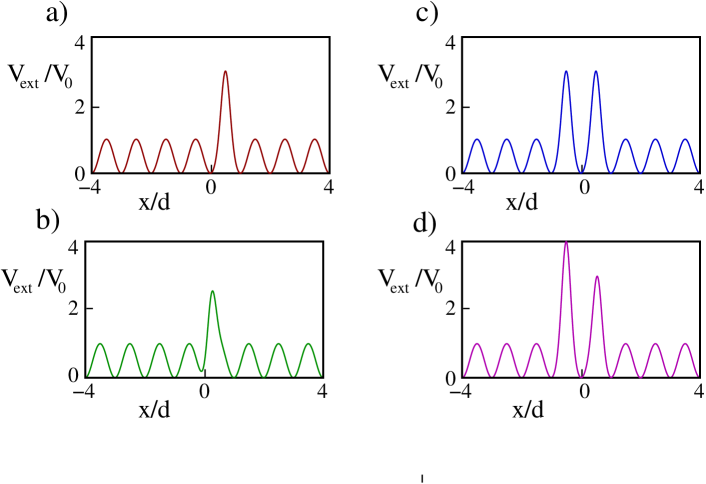
Figure 1: External potential $V_{ext}$ (in units of $V_{0}$) as a function of $x$ (in units of $d$) for different values of $V_{1}/V_{0}$ and $V_{2}/V_{0}$ (with $\sigma=0.2d$). In panels a) and b), we consider $V_{2}=0$ so that only two hopping parameters are altered: panel a) corresponds to $x_{1}/d=0.5$ and panel b) to $x_{0;1}/d=0.25$ (in both cases $V_{1}/V_{0}=2)$. In panels c) and d), we have $x_{0;1}/d=0.5$ and $x_{-1;0}/d=-0.5$ in both cases, but $V_{1}/V_{0}=V_{2}/V_{0}=2$ for panel c) and $V_{1}/V_{0}=2$, $V_{2}/V_{0}=3$ for panel d).

III Renormalization group flow of the impurity Hamiltonian parameters

In this section, we employ the renormalization group (RG) approach to recover the low-energy long-wavelength physics of a Kondo impurity in an otherwise homogeneous chain. From the RG equations we derive the formula for the invariant length which we eventually identify with $\xi_{K}$. In general, there are two standard ways of realizing the impurity in a spin chain, which we sketch in Fig.2. Specifically, we see that the impurity can be realized as an island containing either an even or odd number of spins. The former case is equivalent to a weak link in an otherwise homogeneous chain, originally discussed in Refs.[Kane and Fisher, 1992b, a] for electronic systems, and reviewed in detail in Ref.[Rommer and Eggert, 2000] in the specific context of spin chains. In this case, which we briefly review in Appendix C, when $\Delta>0$ in Eqs.(4), the impurity corresponds to an irrelevant perturbation, which implies an RG flow of the system towards the fixed point corresponding to two disconnected chains, while for $\Delta<0$ the weak link Hamiltonian becomes a relevant perturbation. Though this implies the emergence of an ”healing length ” for the weak link as an RG invariant length scale, with a corresponding flow towards a fixed point corresponding to the two chains joined into an effectively homogeneous single chain, there is no screening of a dynamical spinful impurity by the surrounding spin degrees of freedom and, accordingly, no screening cloud is detected in this case Rommer and Eggert (2000).

At variance, a dynamical effective impurity screening takes place in the case of an effective spin-1/2 impurity Sørensen and Affleck (1996). In this latter case, at any $\Delta$ such that $-1<\Delta<1$, the perturbative RG approach shows that the disconnected-chain weakly coupled fixed point is ultimately unstable. In fact, the RG trajectories flow towards a strongly coupled fixed point, which we identify with the spin chain two channel Kondo fixed point, corresponding to healing the chain but, at variance with what happens at a weak link for $0<\Delta\leq 1$, this time with the chain healing taking place through an effective Kondo-screening of the magnetic impurity Eggert and Affleck (1992).

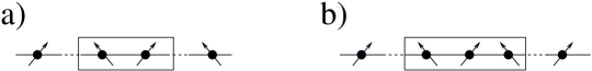
Figure 2: Sketch of two different kinds of central regions in an otherwise uniform spin chain, respectively realizing an effective weak-link impurity (a)), and an effective spin-1/2 impurity (b)).

A region containing an odd number of sites typically has a twofold degenerate groundstate and, therefore, is mapped onto an effective spin-1/2 impurity ${\bf S}_{\bf G}$. The corresponding impurity Hamiltonian in Eq.(29) takes the form of the Kondo spin-chain interaction Hamiltonian for a central impurity in an otherwise uniform spin chain Laflorencie et al. (2008). To employ the bosonization formalism of appendix C to recover the RG flow of the impurity coupling strength, we resort to Eq.(49), corresponding to the bosonized spin Kondo Hamiltonian $H_{K}$ given by

$$H_{K}=\sum_{\alpha=L,R}\left\{-J_{\alpha}^{{}^{\prime}}[S_{0}^{+}e^{-\frac{i}{\sqrt{2}}\Phi_{\alpha}(0)}+S_{0}^{-}e^{\frac{i}{\sqrt{2}}\Phi_{\alpha}(0)}]+J_{z\alpha}^{{}^{\prime}}S_{0}^{z}\frac{1}{\sqrt{2}\pi}\frac{\partial\Theta_{\alpha}(0)}{\partial x}\right\}\>\>\>\>.$$ (6)

The RG equations describing the flow of the impurity coupling strength can be derived by means of standard techniques for Kondo effect in spin chains Furusaki and Hikihara (1998) and, in particular, by considering the fusion rules between the various operators entering $H_{K}$ in Eq.(6). In doing so, in principle additional, weak link-like, operators describing direct tunneling between the two chains can be generated, such as, for instance, a term $\propto e^{\frac{i}{\sqrt{2}}[\Phi_{L}(0)-\Phi_{R}(0)]}$, with scaling dimension $h_{A}=\frac{1}{g}$. However, one may safely neglect a term as such, since, for $g<1$, it corresponds to an additional irrelevant boundary operator that has no effects on the RG flow of the running couplings appearing in $H_{K}$. For $g\geq 1$ it becomes marginal, or relevant, but still subleading, compared to the terms $\propto J_{\alpha}^{{}^{\prime}}$, as we discuss in the following and, therefore, it can again be neglected for the purpose of working out the RG flow of the boundary couplings. This observation effectively enables us to neglect operators mixing the _L and the _R couplings with each other and, accordingly, to factorize the RG equations for the running couplings with respect to the index _α.

More in detail, we define the dimensionless variables $G_{\alpha}(\ell)$ and $G_{z,\alpha}(\ell)$ as

$$G_{\alpha}(\ell)=\left(\frac{\ell}{\ell_{0}}\right)^{1-\frac{1}{2g}}\frac{J_{\alpha}^{{}^{\prime}}}{J}\,\,\,\,\,\,\,\,{\rm and}\,\,\,\,\,\,\,\,G_{z,\alpha}(\ell)=\frac{J_{z\alpha}^{{}^{\prime}}}{J}\>\>\>\>,$$ (7)

(see Appendix B for a discussion on the estimate of the reference length $\ell_{0}$) with $\alpha=L,R$.

The RG equations for the running couplings are given by

$$\frac{dG_{\alpha}(\ell)}{d\ln(\frac{\ell}{\ell_{0}})} = h_{g}G_{\alpha}(\ell)+G_{\alpha}(\ell)G_{z,\alpha}(\ell)$$

$$\frac{dG_{z\alpha}(\ell)}{d\ln(\frac{\ell}{\ell_{0}})} = G_{\alpha}^{2}(\ell)\>\>\>\>,$$ (8)

with $h_{g}=1-1/(2g)$. For the reasons discussed above, the RG equations in Eq.(8) for the _L- and the _R-coupling strengths are decoupled from each other. In fact, they are formally identical to the corresponding equations obtained for a single link impurity placed at the end of the chain (“Kondo side impurity”) Laflorencie et al. (2008). At variance with this latter case, as argued by Affleck and Eggert Eggert and Affleck (1992), in our specific case of a ”Kondo central impurity” the scenario for what concerns the possible Kondo-like fixed points is much richer, according to whether $G_{L}(\ell_{0})\neq G_{R}(\ell_{0})$ (“asymmetric case”), or $G_{L}(\ell_{0})=G_{R}(\ell_{0})$ (“symmetric case”), as we discuss below.

To integrate Eqs.(8), we define the reduced variables $X_{\alpha}(\ell)\equiv G_{\alpha}(\ell)$ and $X_{z,\alpha}(\ell)=G_{z,\alpha}(\ell)+1-\frac{1}{2g}$ for $\alpha=L,R$ (since the equations for the two values of $\alpha$ are formally equal to each other, from now on we will understand the index $\alpha$). As a result, one gets

$$\frac{dX(\ell)}{d\ln(\frac{\ell}{\ell_{0}})}=X(\ell)X_{z}(\ell);\,\,\,\,\,\,\,\,\frac{dX_{z}(\ell)}{d\ln(\frac{\ell}{\ell_{0}})}=X^{2}(\ell).$$ (9)

Equations (9) coincide with the RG equations obtained for the Kosterlitz-Thouless phase transition Itzykson and Drouffe (1998). To solve them, we note that the quantity

$$\kappa=X_{z}^{2}(\ell)-X^{2}(\ell)\;\;\;\;,$$ (10)

is invariant along the RG trajectories. In terms of the microscopic parameters of the BH Hamiltonan one gets $\kappa=\kappa(\ell_{0})=(V/J-3J^{{}^{\prime}2}/(4UJ)+1-1/(2g))^{2}-(J^{{}^{\prime}}/J)^{2}$. To avoid the onset of Mott-insulating phases, we have to assume that the interaction is such that $g>1/2$. This implies $h_{g}>0$ and $X_{z}(\ell_{0})>0$: thus, we assume $X(\ell_{0}),X_{z}(\ell_{0})>0$. This means that the RG trajectories always lie within the first quarter of the $(X,X_{z})$-parameter plane and, in particular, that the running couplings always grow along the trajectories.

Using the constant of motion in Eq.(10), Eqs.(9) can be easily integrated. As a result, one may estimate the RG invariant length scale $\ell_{*}$ defined by the condition that, at the scale $\ell\sim\ell_{*}$, the perturbative calculation breaks down (which leads us to eventually identify $\ell_{*}$ with $\xi_{K}$). As this is signaled by the onset of a divergence in the running parameter $X(\ell)$ Giuliano et al. (2016), one may find the explicit formulas for $\ell_{*}$, depending on the sign of $\kappa$, as detailed below:

• $\kappa=0$. In this case, as the symmetry at $\ell=\ell_{0}$ between $K$ and $X_{z}$ is preserved along the RG trajectories, it is enough to provide the explicit solution for $X_{z}(\ell)(=X(\ell))$, which is given by

  $$X_{z}(\ell)=\frac{X_{z}(\ell_{0})}{1-X_{z}(\ell_{0})\ln(\frac{\ell}{\ell_{0}})}\>\>\>\>.$$ (11)

  From Eq.(11), one obtains

  $$\ell_{*}\sim\ell_{0}\exp\left[\frac{1}{X_{z}(\ell_{0})}\right]\>\>\>,$$ (12)

  which is the familiar result one recovers for the ”standard” Kondo effect in metals Sørensen and Affleck (1996).

• $\kappa<0$. In this case, the explicit solution of Eqs.(9) is given by

  $$X_{z}(\ell) = \sqrt{-\kappa}\tan\left\{{\rm atan}\left[\frac{X_{z}(\ell_{0})}{\sqrt{-\kappa}}\right]+\sqrt{-\kappa}\ln\left(\frac{\ell}{\ell_{0}}\right)\right\}$$

  $$X(\ell) = \sqrt{-\kappa+X_{z}^{2}(\ell)}\>\>\>\>,$$ (13)

  which yields

  $$\ell_{*}\sim\ell_{0}\exp\left[\frac{\pi-2\>{\rm atan}(\frac{X_{z}(\ell_{0})}{\sqrt{|\kappa|}})}{2\sqrt{|\kappa|}}\right]\>\>\>\>.$$ (14)

• $\kappa>0$. In this case one obtains

  $$X_{z}(\ell) = -\sqrt{\kappa}\left\{\frac{[X_{z}(\ell_{0})-\sqrt{\kappa}]\left(\frac{\ell}{\ell_{0}}\right)^{2\sqrt{\kappa}}+[X_{z}(\ell_{0})+\sqrt{\kappa}]}{[X_{z}(\ell_{0})-\sqrt{\kappa}]\left(\frac{\ell}{\ell_{0}}\right)^{2\sqrt{\kappa}}-[X_{z}(\ell_{0})+\sqrt{\kappa}]}\right\}$$

  $$X(\ell) = \sqrt{-\kappa+X_{z}^{2}(\ell)}\>\>\>\>.$$ (15)

  As a result, we obtain

  $$\ell_{*}\sim\ell_{0}\left\{\frac{X_{z}(\ell_{0})+\sqrt{\kappa}}{X_{z}(\ell_{0})-\sqrt{\kappa}}\right\}^{\frac{1}{2\sqrt{\kappa}}}\>\>\>\>.$$ (16)

To provide some realistic estimates of $\ell_{*}$, in Fig.3 we plot $\ell_{*}/\ell_{0}$ as a function of the repulsive interaction potential $V$, keeping fixed all the other system parameters (see the caption for the numerical values of the various parameters). The two plots we show correspond to different values of $J^{{}^{\prime}}$. We see that, as expected, at any value of $V/J$, $\ell_{*}$ decreases on increasing $J^{{}^{\prime}}$. We observe that with realistically small values of $V/J$, say between $0$ and $0.5$, one has a value of the Kondo length order of $20$ sites (for $J^{\prime}/J=0.2$) and $5$ sites (for $J^{\prime}/J=0.6$), that should detectable from experimental data.

Also, we note a remarkable decrease of $\ell_{*}$ with $V/J$ and, in particular, a finite $\ell_{*}$ even at extremely small values of $V$, which correspond to negative values of $J_{z}^{{}^{\prime}}$ and, thus, to an apparently ferromagnetic Kondo coupling between the impurity and the chain. In fact, in order for the Kondo coupling to be antiferromagnetic, and, thus, to correspond to a relevant boundary perturbation, one has to either have both $J^{{}^{\prime}}$ and $J_{z}^{{}^{\prime}}$ positive, or the former one positive, the latter negative. In our case, the RG equations in Eqs.(9), show how the $\beta$-function for the running coupling $X(=G)$ is proportional to $X_{z}G$, rather than to $G_{z}G$. Thus, what matters here is the fact that $X_{z}-G_{z}=1-\frac{1}{2g}>0$, which makes $X_{z}(\ell_{0})$ positive even though $G_{z}(\ell_{0})$ is negative. As a result, even when both $J^{{}^{\prime}}$ and $J_{z}^{{}^{\prime}}$ are negative as it may happen, for instance, if one starts from a BH model with $V\sim 0$, one may still recover a Kondo-like RG flow and find a finite $\ell_{*}$, as evidenced by the plots in Fig.3.

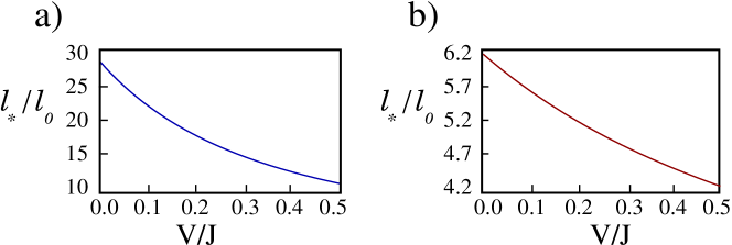
Figure 3: $\ell_{*}/\ell_{0}$ as a function of $V/J$ for $0\leq V/J\leq 0.5$. The other parameters are chosen so that $U/J=4$ and $J^{\prime}/J=0.2$ (panel a)), and $J^{\prime}/J=0.6$ (panel b)). As discussed in Appendix B, $\ell_{0}$ is of order of the lattice spacing $d$.

Being an invariant quantity along the RG trajectories, here $\ell_{*}$ plays the same role as $\xi_{K}$ in the ordinary Kondo effect, that is, once the RG trajectories for the running strengths are constructed by using the system size $\ell$ as driving variable, all the curves are expected to collapse onto each other, provided that, at each curve, $\ell$ is rescaled by the corresponding $\ell_{*}$ Sørensen and Affleck (1996); Hewson (1993); Holzner et al. (2009); Florens and Snyman (2015).

In fact, in the specific type of system we are focusing onto, that is, an ensemble of cold atoms loaded on a pertinently engineered optical lattice, it may be difficult to vary $\ell$ by, in addition, keeping the filling constant (not to affect the parameters of the effective Luttinger liquid model Hamiltonian describing the system). Yet, one may resort to a fully complementary approach in which, as we highlight in the following, the length $\ell$, as well as the filling $f$, are kept fixed and, taking advantage of the scaling properties of the Kondo RG flow, one probes the scaling properties by varying $\ell_{*}$. Indeed, from our Eqs.(12,14,16), one sees that in all cases of interest, the relation between $\ell_{*}$ and the microscopic parameters characterizing the impurity Hamiltonian is known. As a result, one can in principle arbitrarily tune $\ell_{*}$ at fixed $\ell$ by varying the tunable system parameter. As we show in the following, this provides an alterative way for probing scaling behavior, more suitable to an optical lattice hosting a cold atom condensate. In order to express the integrated RG flow equations for the running parameters as a function of $\ell$ and $\ell_{*}$, it is sufficient to integrate the differential equations in Eqs.(9) from $\ell_{*}$ up to $\ell$. As a result, one obtains the following equations:

• For $\kappa=0$:

  $$X(\ell)=X_{z}(\ell)=\frac{X_{z}(\ell_{0})}{-\ln(\frac{\ell}{\ell_{*}})}\>\>\>\>;$$ (17)

• For $\kappa<0$:

  $$X_{z}(\ell) = \sqrt{-\kappa}\tan\left\{\frac{\pi}{2}-\sqrt{-\kappa}\ln\left(\frac{\ell_{*}}{\ell}\right)\right\}$$

  $$X(\ell) = \sqrt{-\kappa+X_{z}^{2}(\ell)}\>\>\>\>;$$ (18)

• For $\kappa>0$:

  $$X_{z}(\ell) = \sqrt{\kappa}\left\{\frac{\left(\frac{\ell_{*}}{\ell}\right)^{2\sqrt{\kappa}}+}{\left(\frac{\ell_{*}}{\ell}\right)^{2\sqrt{\kappa}}-1}\right\}$$

  $$X(\ell) = \sqrt{-\kappa+X_{z}^{2}(\ell)}\>\>\>\>.$$ (19)

From Eqs.(17,18,19), one therefore concludes that, once expressed in terms of $\ell/\ell_{*}$, the integrated RG flow for the running coupling strengths only depends on the parameter $\kappa$. Curves corresponding to the same values of $\kappa$ just collapse onto each other, independently of the values of all the other parameters.

We pause here for an important comment. As discussed in Laflorencie et al. (2008), in the spin chain realization of the Kondo model, one exactly retrieves the equation of the conventional Kondo effect at $g=1/2$ only after adding a frustrating second-neighbor interaction, thus resorting to the so-called $J_{1}-J_{2}$ model Hamiltonian. In principle, the same would happen for the $XXX$-spin chain with nearest-neighbor interaction only, except that, strictly speaking, the correspondence is exactly realized only in the limit of an infinitely long chains. In the case of finite chains, the presence of a marginally irrelevant Umklapp operator may induce finite-size violations from Kondo scaling which, as stated above, disappear in the thermodynamic limit. Yet, as this point is mostly of interest because it may affect the precision of numerical calculations, we do not address it here and refer to Ref.[Laflorencie et al., 2008] for a detailed discussion of this specific topic.

Another important point to stress is that, strictly speaking, we have so far neglected the possible effects of the asymmetry ($J_{L}^{{}^{\prime}}\neq J_{R}^{{}^{\prime}}$ and $J_{z,L}^{{}^{\prime}}\neq J_{z,R}^{{}^{\prime}}$), versus symmetry ($J_{L}^{{}^{\prime}}=J_{R}^{{}^{\prime}}$ and $J_{z,L}^{{}^{\prime}}=J_{z,R}^{{}^{\prime}}$) in the bare couplings. In fact, the nature of the stable Kondo fixed point reached by the system in the large scale limit deeply depends on whether or not the bare couplings between the impurity and the chains are symmetric, or not. Nevertheless, as we argue in the following, one sees that, while the nature of the Kondo fixed point may be quite different in the two cases (two-channel versus one-channel spin-Kondo fixed point), one can still expect to be able to detect the onset of the Kondo regime and to probe the corresponding Kondo length by looking at the density-density correlations in real space, though the correlations themselves behave differently in the two cases. We discuss at length about this latter point in the next section. Here, we rather discuss about the nature of the Kondo fixed point in the two different situations, starting with the case of symmetric couplings between the impurity and the chains.

When $J_{L}^{{}^{\prime}}=J_{R}^{{}^{\prime}}$ and $J_{zL}^{{}^{\prime}}=J_{zR}^{{}^{\prime}}$, since, to leading order in the running couplings, there is no mixing between the _L- and the _R coupling strengths, the $L-R$ symmetry is not expected to be broken all the way down to the strongly coupled fixed point which, consequently, we identify with the two-channel spin-chain Kondo fixed point, in which the impurity is healed and the two chains have effectively joined into a single uniform chain. Due to the $L-R$ symmetry, one can readily show that all the allowed boundary operators at the strongly coupled fixed point are irrelevant Eggert and Affleck (1992); Furusaki and Hikihara (1998), leading to the conclusion that the two-channel spin-Kondo fixed point is stable, in this case.

Concerning the effects of the asymmetry, on comparing the scale dimensions of the various impurity boundary operators, one expects them to be particularly relevant if the asymmetry is realized in the transverse Kondo coupling strengths, that is, if one has $J_{L}^{{}^{\prime}}\gg J_{R}^{{}^{\prime}}$. We assume that this is the case which, moving to the dimensionless couplings, implies $G_{L}(\ell_{0})\gg G_{R}(\ell_{0})$. Due to the monotonicity of the integrated RG curves, we expect that this inequality keeps preserved along the integrated flow, that is, $G_{L}(\ell)\gg G_{R}(\ell)$ at any scale $\ell\geq\ell_{0}$. In analogy with the standard procedure used with multichannel Kondo effect with non-equivalent channels, one defines $\ell_{*}$ as the scale at which the larger running coupling $G_{L}(\ell)$ diverges, which is the signal of the onset of the nonperturbative regime. Due to the coupling asymmetry, we then expect $G_{R}(\ell_{*})\ll 1$, that is, at the scale $\ell\sim\ell_{*}$, the system may be regarded as a semi-infinite chain at the left-hand side, undergoing Kondo effect with an isolated magnetic impurity, weakly interacting with a second semi-infinite chain, at the right-hand side. To infer the effects of the residual coupling, one may assume that, at $\ell\sim\ell_{*}$, the impurity is “re-absorbed” in the left-hand chain Eggert and Affleck (1992); Furusaki and Hikihara (1998), so that this scenario will consist of the left-hand chain, with one additional site, connected with a link of strength $\sim G_{R}(\ell_{*})$ to the endpoint of the right-hand chain. Within the bosonization approach, the weak link Hamiltonian is given by Kane and Fisher (1992a)

$$V_{B}^{\rm Asym}\sim-G_{R}(\ell_{*})e^{\frac{i}{\sqrt{2}}[\Phi_{L}(0)-\Phi_{R}(0)]}+{\rm h.c.}\>\>\>\>.$$ (20)

$V_{B}^{\rm Asym}$ has scaling dimension $\frac{1}{g}$. Depending on whether $g>1$, or $g<1$, it can therefore be either relevant, or irrelevant (or marginal if $g=1$). When relevant, it drives the system towards a fixed point in which the weak link is healed. When irrelevant, the fixed point corresponds to the two disconnected chains. In either case, the residual flow takes place after the onset of Kondo screening. We therefore conclude that Kondo screening takes place in the left-hand chain only and, accordingly, one expects to be able to probe $\ell_{*}$ by just looking at the real space density-density correlations in that chain only. From the above discussion we therefore conclude that Kondo effect is actually realized at a chain with an effective spin-1/2 impurity whether or not the impurity couplings to the chains are symmetric, or not, though the fixed point the system is driven to along the RG trajectories can be different in the two cases.

IV Density-density correlations and measurement of the Kondo length

In analogy to the screening length $\xi_{K}$ in the standard Kondo effect Nozières (1974, 1978), in the spin chain realization of the effect, the screening length $\ell_{*}$ is identified with the typical size of a cluster of spins fully screening the moment of the isolated magnetic impurity, either lying at one side of the impurity itself (in the one-channel version of the effect-side impurity at the end of a single spin chain), or surrounding the impurity on both sides (two channel version of the effect-impurity embedded within an otherwise uniform chain).

So far, $\ell_{*}$ showed itself as quite an elusive quantity to experimentally detect, both in electronic Kondo effect, as well as in spin Kondo effect Affleck (arXiv:0911.2209). In this section, we propose to probe $\ell_{*}$ in the effective spin-1/2 $XXZ$ chain describing the BH model, by measuring the integrated real-space density-density correlation functions. Real-space density-density correlations in atomic condensates on an optical lattice can be measured with a good level of accuracy (see e.g. Refs.[Pethick and Smith, 2002; Greiner et al., 2001].) Given the mapping between the BH- and the spin-1/2 $XXZ$ spin Hamiltonian, real-space density-density correlation functions are related via Eq.(3) to the correlation functions of the $z$-component of the effective spin operators in the $XXZ$-Hamiltonian (local spin-spin susceptibility), which eventually enables us to analytically compute the correlation function within spin-1/2 $XXZ$ spin chain Hamiltonian framework. The idea of inferring informations on the Kondo length by looking at the scaling properties of the real-space local spin susceptibility was put forward in Ref.[Barzykin and Affleck, 1996]. In the specific context of lattice model Hamiltonians, the integrated real-space correlations have been proposed as a tool to extract $\xi_{K}$ in a quantum dot, regarded as a local Anderson model, interacting with itinerant lattice spinful fermions Holzner et al. (2009). Specifically, letting ${\bf S}_{\bf G}$ denote the spin of the isolated spin-1/2 impurity and ${\bf S}_{j}$ the spin operator in the site $j$, assuming that the impurity is located at one of the endpoints of the chain and that the whole model, including the term describing the interaction between ${\bf S}_{\bf G}$ and the spins of the chain, is spin-rotational invariant, one may introduce the integrated real-space correlation function ${\bf\Sigma}(x)$, defined as Holzner et al. (2009)

$${\bf\Sigma}(x)=1+\sum_{y=1}^{x}\left[\frac{\langle{\bf S}_{\bf G}\cdot{\bf S}_{y}\rangle}{\langle{\bf S}_{\bf G}\cdot{\bf S}_{\bf G}\rangle}\right]\>\>\>\>.$$ (21)

The basic idea is that the first zero of ${\bf\Sigma}(x)$ one encounters in moving from the location of the impurity, identifies the portion of the whole chains containing the spins that fully screen ${\bf S}_{\bf G}$. Once one has found the solution of the equation ${\bf\Sigma}(x=x_{*})=0\>,$ one therefore naturally identifies $x_{*}$ with $\ell_{*}$. It is important to stress that this idea equally applies whether one is considering the spin impurity at just one side of the chain (one-channel spin chain Kondo), or embedded within the chain (two-channel spin chain Kondo). Thus, while in the following we mostly consider the two-channel case, we readily infer that our discussion applies also to the one-channel case.

To adapt the approach of Ref.[Holzner et al., 2009] to our specific case, first of all, since our impurity is located at the center of the chain, one has to modify the definition of ${\bf\Sigma}(x)$ so to sum over $j$ running from $-x$ to $x$. In addition, in our case both the bulk spin-spin interaction, as well as the effective Kondo interaction with the impurity, are not isotropic in the spin space. This requires modifying the definition of ${\bf\Sigma}(x)$, in analogy to what is done in Ref.[Holzner et al., 2009] in the case in which an applied magnetic field breaks the spin rotational invariance. Thus, to probe $\ell_{*}$ we use the integrated $z$-component of the spin correlation function, ${\bf\Sigma}_{z}(x)$, defined as

$${\bf\Sigma}_{z}(x)=1+\sum_{y=-x}^{x}\left[\frac{\langle S_{\bf G}^{z}S_{y}^{z}\rangle-\langle S_{\bf G}^{z}\rangle\langle S_{y}^{z}\rangle}{\langle S_{\bf G}^{z}S_{\bf G}^{z}\rangle-\langle S_{\bf G}^{z}\rangle^{2}}\right]\>\>\>\>.$$ (22)

In general, estimating $\ell_{*}$ from ${\bf\Sigma}_{z}(x)$ would require exactly computing the spin-spin correlation functions by means of a numerical technique, such as it is done in Ref.[Holzner et al., 2009] – nevertheless one in general expects that the estimate of $\ell_{*}$ obtained using perturbative RG differs by a factor order of $1$ from the one obtained by nonperturbative, numerical means. For the purpose of showing the consistency between the estimate of $\ell_{*}$ from the spin-spin correlation functions and the results from the perturbative analysis of Sec.III, one therefore expects it to be sufficient to resort to a perturbative (in $J_{z}^{{}^{\prime}},J^{\prime}$) calculation of ${\bf\Sigma}_{z}(x)$, eventually improved by substituting the bare coupling strengths with the running ones, computed at an appropriate scale Sørensen and Affleck (1996). To leading order in the impurity couplings, we obtain

$$\langle S_{\bf G}^{z}S_{y}^{z}\rangle = -J_{z,R}^{{}^{\prime}}\>\int_{0}^{\infty}\>d\tau\>G_{z,z}(y,1;\tau|\ell)\>,\;(y>0)$$

$$\langle S_{\bf G}^{z}S_{y}^{z}\rangle = -J_{z,L}^{{}^{\prime}}\>\int_{0}^{\infty}\>d\tau\>G_{z,z}(y,1;\tau|\ell)\>,\;(y<0)\>\>\>\>,$$ (23)

with the finite-$\tau$ correlation function $G_{z,z}(x,x^{\prime};\tau|\ell)$ defined in Eq.(53). To incorporate scale effects in the result of Eq.(23), we therefore replace the bare impurity coupling strengths with the running ones we derived in Sec.III, computed at an appropriate length scale, which we identify with the size $x$ of the spin cluster effectively contributing to impurity screening. Therefore, referring to the dimensionless running coupling $X_{z}(\lambda)$ defined in Eqs.(8), we obtain

$${\bf\Sigma}_{z}(x) = 1-\frac{8J_{z}^{{}^{\prime}}(x)\ell}{\pi u}\>\sum_{y=1}^{x}\>\int_{0}^{\infty}\>dw\>G_{z,z}\left(y,1;\frac{\pi uw}{\ell}\biggr{|}\ell\right)$$ (24)

$$= 1-8\varphi(\Delta)\left[X_{z}(x)+\frac{1}{2g}-1\right]\>\ell\>\sum_{y=1}^{x}\>\int_{0}^{\infty}\>dw\>G_{z,z}\left(y,1;\frac{\pi uw}{\ell}\biggr{|}\ell\right)\>\>\>\>,$$

with $\varphi(\Delta)$ given by

$$\varphi(\Delta)=\frac{{\rm arcos}\left(\frac{\Delta}{2}\right)}{\pi^{2}\sqrt{1-\left(\frac{\Delta}{2}\right)^{2}}}\>\>\>\>.$$ (25)

Remarkably, $\varphi(\Delta)\to 1$ as $\Delta\to 0$. In Fig.4, we show ${\bf\Sigma}_{z}(x)$ vs. $x$ (only the positive part of the graph) for two paradigmatic situations: in Fig.4a) we consider the absence of nearest-neighbor ”bare” density-density interaction ($V=0$). In Fig.4b) we consider a rather large, presently not straightforward to be implemented in experiments, value of $V$ ($V/J\sim 2.2$) to show the results for the Kondo length with a positive value of the $XXZ$ anisotropy parameter. We see that there is not an important dependence of the Kondo length upon $V$, since the main parameter affecting $\ell_{*}$ is actually given by $J^{\prime}/J$.

From the analysis of Ref.[Giuliano et al., 2013], one sees that, even at $V=0$, a nonzero attractive density-density interaction between nearest-neighboring sites of the chain is actually induced by higher order (in $t/U$) virtual processes, which implies that, for $V=0$, $g$ keeps slightly higher than $1$. At variance, for finite $V$, $g$ can be either larger, or smaller than $1$, as it is the case in the plot in Fig.4b). In both cases we see the effect of ”Friedel-like” oscillations in the density-density correlation, which eventually conspire to set ${\bf\Sigma}_{z}(x)$ to $0$ at a scale $x\sim\ell_{*}$ (see the caption of the figures for more details on the numerical value of the various parameters).

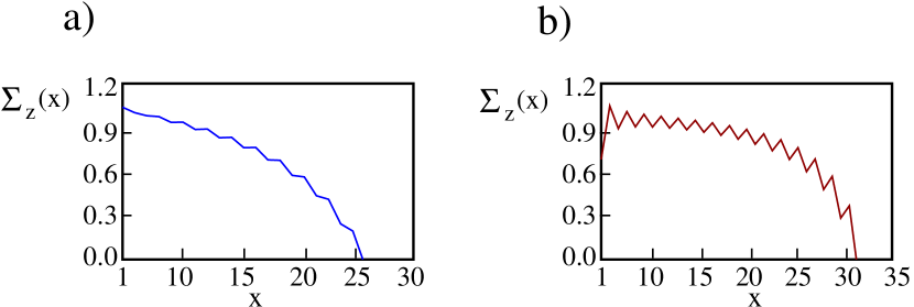
Figure 4: a): Plot of ${\bf\Sigma}_{z}(x)$ vs. $x$ for $U/J=4$, $V=0$ (corresponding to $\Delta=-0.1875$) and $J^{\prime}/J=0.2$. From the plot one infers $\ell_{*}\sim 26$, which is in good agreement with the value obtained from the plot in Fig.3a). b): Same as before, but with $V/J=2.1875$ (corresponding to $\Delta=0.2$) and $J^{\prime}/J=0.1$. As expected, the lower value of $J^{\prime}$ yields a larger $\ell_{*}\sim 32$.

In general, Eq.(24) has to be regarded within the context of the general scaling theory for ${\bf\Sigma}_{z}(x)$ Sørensen and Affleck (1996). In our specific case, at variance with what happens in the ”standard” Kondo problem of itinerant electrons in a metal magnetically interacting with an isolated impurity Sørensen and Affleck (1996), the boundary action in Eq.(49) contains terms that are relevant as the length scale grows. In general, in this case a closed-form scaling formula for physical quantities cannot be inferred from the perturbative results, due to the proliferation of additional terms generated at higher orders in perturbation theory Amit and Martin-mayor (2005). Nevertheless, here one can still recover a pertinently adapted scaling equation, as only dimensionless contributions to $S^{B}_{\bf G}$ effectively contribute ${\bf\Sigma}_{z}(x)$ to any order in perturbation theory. The point is that, as we are considering a boundary operator in a bosonized theory in which the fields $\Phi_{L,R}(x,\tau)$ obey Neumann boundary conditions at the boundary, the fields $\Theta_{L.R}(0,\tau)$ appearing in the bosonized formula for $S_{1,L}^{z},S_{1,R}^{z}$ in Eqs.(45) are pinned at a constant for any $\tau$. As a result, the corresponding contribution to the boundary interaction reduces to the one in Eq.(49), which is purely dimensionless and, therefore, marginal. As for what concerns the contribution $\propto J^{{}^{\prime}}_{L,R}$, it is traded for a marginal one once one uses as running couplings the rescaled variables $X_{L}$ and $X_{R}$, rather than $J^{\prime}_{L},J^{\prime}_{R}$. Now, from Eqs.(45) we see that the bosonization formula for $S_{j}^{z}$ contains a term that has dimension $d_{1}=1$ and a term with dimension $d_{2}=(2g)^{-1}$. Taking into account the dynamics of the degrees of freedom of the chains comprised over a segment of length $x$, we therefore may make the scaling ansatz for ${\bf\Sigma}_{z}$ in the form

$${\bf\Sigma}_{z}[x,\ell,X_{z},X]=\>\tilde{\omega}_{0}\left[\frac{x}{\ell},X_{z},X\right]+\ell^{1-g}\>\tilde{\omega}_{1}\left[\frac{x}{\ell},X_{z},X\right]\>\>\>\>,$$ (26)

with $\omega_{0},\omega_{1}$ scaling functions. Now, we note that, due to the existence of the RG invariant $\kappa$, which relates to each other the running parameters $X_{z}$ and $X$ along the RG trajectories (Eq.(10) in the perturbative regime), we may trade $\tilde{\omega}_{0,1}\left[\frac{x}{\ell},X_{z},X\right]$ for two functions $\omega_{0,1}$ of only $\frac{x}{\ell}$ and $X$. As a final result, Eq.(26) becomes

$${\bf\Sigma}_{z}[x,\ell,X_{z},X]=\omega_{0}\left[\frac{x}{\ell},X_{z}(x)\right]+\ell^{1-g}\>\omega_{1}\left[\frac{x}{\ell},X_{z}(x)\right]\>\>\>\>.$$ (27)

Equation (27) provides the leading perturbative approximation at weak boundary coupling, as it can be easily checked from the explicit formula in Equation (53). Eq.(27) illustrates how the function we explicitly use in our calculation can be regarded as just an approximation to the exact scaling function for ${\bf\Sigma}_{z}(x)$. A more refined analytical treatment might in principle be done by considering higher-order contributions in perturbation theory in $S^{B}_{\bf G}$. Alternatively, one might resort to a fully numerical approach, similar to the one used in Ref.[Holzner et al., 2009]. Yet, due to the absence of an intermediate-coupling phase transition in the Kondo effect Hewson (1993), in our opinion resorting to a more sophisticated approach would improve the quantitative relation between the microscopic ”bare” system parameters and the ones in the effective low-energy long-wavelength model Hamiltonian, without affecting the main qualitative conclusion about the Kondo screening length and its effects.

For this reason, here we prefer to rely on the perturbative RG approach extended to the correlation functions which, as we show before, already provides reliable and consistent results on the effects of the emergence of $\ell_{*}$ on the physical quantities.

The obtained estimate of $\xi_{K}$, although perturbative, provides, via the RG relation $k_{B}T_{K}=\hbar v_{F}/\xi_{K}$, an estimate of the Kondo temperature. When the measurements are done at finite temperature, of course thermal effects affect the estimate of $\xi_{K}$: we anyway expect that if the temperature is much smaller than $T_{K}$, then such effects are negligeable. Considering that $T_{K}$ has been estimated of order of tens of $nK$ Buccheri et al. (2016), and that $T_{K}$ may be increased by increasing $v_{F}$, which may be up to hundreds $nK$, and by increasing $J^{\prime}/J$, we therefore expect that with temperatures smaller than the bandwidth one can safely extract $\xi_{K}$. One should anyway find a compromise since by increasing $J^{\prime}/J$ the Kondo length decreases (and the Kondo effect itself disappears). A systematic study of thermal effects on the estimate of $\xi_{K}$ is certainly an important subject of future work.

V Conclusions

In this paper we have studied the measurement of the Kondo screening length in systems of ultracold atoms in deep optical lattices. Our motivation relies primarily on the fact that the detection of the Kondo screening length from experimentally measurable quantities in general appears to be quite a challenging task. For this reason, we proposed to perform the measurement in cold atom setups, whose parameters can be, in principle, tuned in a controllable way to desired values.

Specifically, after reviewing the mapping between the BH model at half-filling with inhomogenous hopping amplitudes onto a spin chain Hamiltonian with Kondo-like magnetic impurities, we have proposed to extract the Kondo length from a suitable quantity obtained by integrating the real space density-density correlation functions. The corresponding estimates we recover for the Kondo length are eventually found to assume values definitely within the reach of present experiments ($\sim$ tens of lattice sites for typical values of the system parameters). We showed that the Kondo length does not significantly depend on nearest-neighbor interaction $V$, and it mainly depends on the impurity link $J^{\prime}$.

Concerning the Kondo length, a comment is in order for quantum-optics oriented readers: in a typical measurement of the Kondo effect at a magnetic impurity in a conducting metallic host, one has access to the Kondo temperature $T_{K}$, by just looking at the scale at which the resistance (or the conductance, in experiments in quantum dots) bends upwards, on lowering $T$. The very existence of the screening length $\xi_{K}$ is just inferred from the emergence of $T_{K}$ and from the applicability of one-parameter scaling to the Kondo regime, which yields $\xi_{K}=\hbar v_{F}/k_{B}T_{K}$. However the latter relation stems from the validity of the RG approach. Thus, ultimately probing directly $\xi_{K}$ in solid-state samples would correspond to verifying the scaling in the Kondo limit, which is what makes it hard to actually perform the measurement. At variance, as we comment for solid-state oriented readers, in the ultracold gases systems we investigate here, one can certainly study dynamics (e.g., tilting the system) but a stationary flow of atoms cannot be (so far) established, so that the measure of $T_{K}$ may be an hard task to achieve. Rather surprisingly, as our results highlight, it is the Kondo length which can be more easily directly detected in ultracold gases and our corresponding estimates (order of tens of lattice sites) appear to be rather encouraging in this direction.

Several interesting issues deserve in our opinion further work: as first, it would be desirable to compare the perturbative results we obtain in this paper with numerical, nonperturbative findings in the Bose-Hubbard chain, to determine the corresponding correction to the value of $\ell_{*}$. It would be also important to understand the corrections to the inferred value of $\xi_{K}$ coming from finite temperature effects, that should be anyway negligeable for $T$ (much) smaller that $T_{K}$. Even more importantly, we mostly assumed that it is possible to alter the hopping parameters in a finite region without affecting the others. This led us to infer, for instance, the existence of the ensuing even-odd effect – however, having two lasers with $\sigma\ll d$ is a condition that may be straightforwardly implementable. In this case, one has to deal with generic space-dependent hopping amplitudes $t_{j;j+1}$. It would therefore be of interest to address, very likely within a fully numerical approach, the fate of the even-odd effect in the presence of a small modulation in space of the outer hopping terms. In particular, a theoretically interesting issue would be the competition between an extended nonlocal central region and the occurrence of magnetic and/or nonmagnetic impurities in the chain. Another point to be addressed is that an on-site nonuniform potential may in principle be present (event though its effect may be reduced by hard wall confining potentials) and an interesting task is to determine the interplay between the Kondo length and the length scale of such an additional potential.

In conclusion, we believe that our results show that the possible realization of the setup proposed in this paper could pave the way to the study of magnetic impurities and, in perspective, to the experimental implementation of ultracold realizations of Kondo lattices and detection of the Kondo length, providing, at the same time, a chance for studying several interesting many-body problems in a controllable way.

We thank L. Dell’Anna, A. Nersesyan, A. Papa, and D. Rossini for valuable discussions. A.T. acknolweldges support from talian Ministry of Education and Research (MIUR) Progetto Premiale 2012 ABNANOTECH - ATOM-BASED NANOTECHNOLOGY.

Appendix A Effective weak link- and Kondo-Hamiltonians for a spin-1/2 $XXZ$ spin chain

In this appendix we review the description of a region G, singled out by weakening two links in a $XXZ$ spin chain, in terms of an effective low-energy Hamiltonian $H_{\bf G}$. In particular, we show how, depending on whether the number of sites containined within G is odd, or even, either $H_{\bf G}$ coincides with the Kondo Hamiltonian $H_{K}$ in Eq.(5), or it describes a weak link between two ”half-chains” Glazman and Larkin (1997); Giuliano and Sodano (2005).

In general, Kondo effect in spin-1/2 chains has been studied for an isolated magnetic impurity (the “Kondo spin”), which may either lie at the end of the chain (boundary impurity), or at its middle (embedded impurity) Eggert and Affleck (1992); Furusaki and Hikihara (1998). In the former case, the impurity can be realized by “weakening” one link of the chain, in the latter case, instead, it can be realized by weakening two links in the body of the chain. Following the discussion in Sec.III of the main text, here we mostly focus on the latter case. In general, in a spin chain, impurities may be realized as extended objects, as well, that is, as regions containing two, or more, sites. Whether the Kondo physics is realized, or not, does actually depend on whether the level spectrum of the isolated impurity takes, or not, a degenerate ground state. A doubly degenerate ground state is certainly realized in an extended region with an odd number of sites, without explicit breaking of “spin inversion” symmetry (that is, in the absence of local “magnetic fields”). For instance, let us consider a central region realized by three sites ($j=-1,0,1$), lying between the weak links. Let the central region Hamiltonian be given by

$$H_{3J}^{\rm Middle}=-J\left(S_{-1}^{+}S_{0}^{-}+S_{0}^{+}S_{1}^{-}+{\rm h.c.}\right)+J^{z}\left(S_{-1}^{z}S_{0}^{z}+S_{0}^{z}S_{1}^{z}\right)\>\>\>\>,$$ (28)

and let the central region be connected to the left-hand chain (which, as in the main text, we denote by the label _L), and to the right-hand chain (denoted by the label _R) with the coupling Hamiltonian

$$H_{\rm Coupling}=-\left(J_{L}^{{}^{\prime}}S_{1,L}^{+}S_{-1}^{-}+J_{R}^{{}^{\prime}}S_{1,R}^{+}S_{1}^{-}+{\rm h.c.}\right)+\left(J_{z,L}^{{}^{\prime}}S_{1,L}^{z}S_{-1}^{z}+J_{z,R}^{{}^{\prime}}S_{1,R}^{z}S_{1}^{z}\right)\>\>\>\>.$$ (29)

A simple algebraic calculation shows that the ground state of $H_{3J}^{\rm Middle}$ is doubly degenerate and consists of the spin-1/2 doublet given by

$$|\frac{1}{2}\rangle_{2}=\frac{1}{\sqrt{2}}\{\sin(\frac{\theta}{2})[\uparrow\uparrow\downarrow\rangle+|\downarrow\uparrow\uparrow\rangle]+\sqrt{2}\cos(\frac{\theta}{2})|\uparrow\downarrow\uparrow\rangle\}\;\;\;\;,$$ (30)

and

$$|-\frac{1}{2}\rangle_{2}=\frac{1}{\sqrt{2}}\{\sin(\frac{\theta}{2})[\downarrow\downarrow\uparrow\rangle+|\uparrow\downarrow\downarrow\rangle]+\sqrt{2}\cos(\frac{\theta}{2})|\downarrow\uparrow\downarrow\rangle\}\;\;\;\;,$$ (31)

with

$$\cos(\theta)=\frac{J_{z}}{\sqrt{2J^{2}+J_{z}}}\;\;\;,\;\;\cos(\theta)=\frac{\sqrt{2}J}{\sqrt{2J^{2}+J_{z}}}\>\>\>\>,$$ (32)

whose energy is given by $E_{2}^{\frac{1}{2}}=-J_{z}-\sqrt{J_{z}^{2}+2J^{2}}$. Defining an effective spin-1/2 operator for the central region, ${\bf S}_{G}$, as

$$S_{G}^{+}\equiv|\frac{1}{2}\rangle_{2}~{}_{2}\langle-\frac{1}{2}|\>\>\>,\>\>S_{G}^{z}\equiv\frac{1}{2}\sum_{b=\pm 1}b|b\frac{1}{2}\rangle_{2}~{}_{2}\langle b\frac{1}{2}|\>\>\>\>,$$ (33)

allows to rewrite $H_{3J}^{\rm Middle}+H_{\rm Coupling}$ as

$$V_{B}^{\rm 3J}=-\{[J^{{}^{\prime}}_{L}\sin(\theta)S_{1,L}^{+}+J^{{}^{\prime}}_{R}S_{1,R}^{+}]S_{G}^{-}+[J^{{}^{\prime}}_{L}S_{1,L}^{-}+J^{{}^{\prime}}_{R}S_{1,R}^{-}]S_{G}^{+}\}+\cos(\theta)[J_{z,L}^{{}^{\prime}}S_{1,L}^{z}+J_{z,R}^{{}^{\prime}}S_{1,R}^{z}]S_{G}^{z}\>\>\>\>.$$ (34)

Thus, we see that we got back to the spin-1/2 spin-chain Kondo Hamiltonian, with a renormalization of the boundary couplings, according to

$$J^{{}^{\prime}}_{L(R)}\longrightarrow J^{{}^{\prime}}_{L(R)}\sin(\theta)=\frac{\sqrt{2}J^{{}^{\prime}}_{L(R)}J}{\sqrt{2J^{2}+J_{z}}}\;\;\;,\;\;J_{z,L(R)}^{{}^{\prime}}\longrightarrow J_{z,L(R)}^{{}^{\prime}}\cos(\theta)=\frac{J_{z,L(R)}^{{}^{\prime}}J_{z}}{\sqrt{2J^{2}+J_{z}}}\>\>\>\>.$$ (35)

A local magnetic field $h$ may break the ground state degeneracy, thus leading, in principle, to the breakdown of the Kondo effect. However, in analogy to what happens in a Kondo dot in the presence of an external magnetic field Goldhaber-Gordon et al. (1998); Cronenwett et al. (1998); Takagi and Saso (1999), Kondo physics should survive, at least as long as $h\ll{\cal E}_{K}$, with ${\cal E}_{K}(\sim k_{B}T_{K})$ being the typical energy scale associated to the onset of Kondo physics.

At variance, when the central region is made by an even number of sites, the groundstate is not degenerate anymore. As a consequence, the central region should be regarded as a weak link between two chains. For instance, we may consider the case in which the central region is made by two sites. Using for the various parameters the same symbols we used above, performing a SW resummation, we obtain the effective weak link boundary Hamiltonian

$$V_{B}^{\rm 2J}=-\lambda_{\perp}\left(S_{L,1}^{+}S_{R,1}^{-}+S_{R,1}^{+}S_{L,1}^{-}\right)-\lambda_{z}S_{L,1}^{z}S_{R,1}^{z}\>\>\>\>,$$ (36)

with

$$\lambda_{\perp}\sim\frac{(J^{{}^{\prime}})^{2}}{J+2J_{z}}\;\;\;,\;\;\lambda_{z}\sim\frac{(J_{z}^{{}^{\prime}})^{2}}{2J}\>\>\>\>.$$ (37)

Appendix B bosonization approach to impurities in the $XXZ$ spin chain

In this section we review the bosonization approach to the $XXZ$ spin chain as it was originally developed in Refs.[Eggert and Affleck, 1992; Furusaki and Hikihara, 1998]. As a starting point, we consider a single, homogeneous spin-1/2 $XXZ$ spin chain, with $\ell$ sites, obeying open boundary conditions at its endpoints, described by the model Hamiltonian $H_{\rm XXZ}$, given by

$$H_{\rm XXZ}=-J\sum_{j=1}^{\ell-1}\left(S_{j}^{+}S_{j+1}^{-}+S_{j+1}^{+}S_{j}^{-}\right)+J^{z}\sum_{j=1}^{\ell-1}S_{j}^{z}S_{j+1}^{z}\>\>\>\>.$$ (38)

The low-energy, long-wavelength dynamics of such a chain is described Eggert and Affleck (1992) in terms of a spinless, real bosonic field $\Phi(x,\tau)$ and of its dual field $\Theta(x,\tau)$. The imaginary time action for $\Phi$ is given by

$$S_{E}[\Phi]=\frac{g}{4\pi}\>\int_{0}^{\beta}\>d\tau\>\int_{0}^{\ell}\>dx\>\left[\frac{1}{u}\left(\frac{\partial\Phi}{\partial\tau}\right)^{2}+u\left(\frac{\partial\Phi}{\partial x}\right)^{2}\right]\>\>\>\>,$$ (39)

where the constants $g,u$ are given by

$$g=\frac{\pi}{2(\pi-{\rm arccos}(\frac{\Delta}{2}))}\;\;\;,\;\;u=v_{f}\left[\frac{\pi}{2}\frac{\sqrt{1-(\frac{\Delta}{2})^{2}}}{{\rm arccos(\frac{\Delta}{2})}}\right]\;\;\;\;,$$ (40)

with $v_{f}=2dJ$, $d$ being the lattice step, and $\Delta=J^{z}/J$. The fields $\Phi$ and $\Theta$ are related to each other by the relations $\frac{\partial\Phi(x,\tau)}{\partial x}=\frac{1}{u}\frac{\partial\Theta(x,\tau)}{\partial x}$, and $\frac{\partial\Theta(x,\tau)}{\partial x}=\frac{1}{u}\frac{\partial\Phi(x,\tau)}{\partial x}$. A careful bosonization procedure shows that, in addition to the free Hamiltonian in Eq.(39), an additional Sine-Gordon, Umklapp interaction arises, given by

$$H_{\rm L}^{\rm SG}=-G_{U}\int_{0}^{\ell}\>dx\>\cos[2\sqrt{2}\Theta(x)]\>\>\>\>.$$ (41)

Since the scaling dimension of $H_{\rm L}^{\rm SG}$ is $h_{U}=4g$, it will be always irrelevant within the window of values of $g$ we are considering here, that is, $1/2<g$. In fact, $H_{\rm L}^{\rm SG}$ becomes marginally irrelevant at the “Heisenberg point”, $g=1/2$, which deserves special attention Laflorencie et al. (2008), though we do not consider it here. Within the continuous bosonic field framework, the open boundary conditions of the chain are accounted for by imposing Neumann-like boundary conditions on the field $\Phi(x,\tau)$ at both boundaries Giuliano and Sodano (2005, 2007, 2009); Cirillo et al. (2011), that is

$$\frac{\partial\Phi(0,\tau)}{\partial x}=\frac{\partial\Phi(\ell,\tau)}{\partial x}=0\>\>\>\>.$$ (42)

Equation (42) implies the following mode expansions for $\Phi(x,\tau)$ and $\Theta(x,\tau)$

$$\Phi(x,\tau)=\sqrt{\frac{2}{g}}\left\{q-\frac{i\pi u\tau}{\ell}P+i\sum_{n\neq 0}\frac{\alpha(n)}{n}\cos\left[\frac{\pi nx}{\ell}\right]e^{-\frac{\pi n}{\ell}u\tau}\right\}$$

$$\Theta(x,\tau)=\sqrt{2g}\left\{\theta+\frac{\pi x}{\ell}P+\sum_{n\neq 0}\frac{\alpha(n)}{n}\sin\left[\frac{\pi nx}{\ell}\right]e^{-\frac{\pi n}{\ell}u\tau}\right\}\>\>\>\>,$$ (43)

with the normal modes satisfying the algebra

$$[q,P]=i\;\;\;,\;\;[\alpha(n),\alpha(n^{\prime})]=n\delta_{n+n^{\prime},0}\>\>\>\>.$$ (44)

The bosonization procedure allows for expressing the spin operators in terms of the $\Phi$- and $\Theta$-fields. The result is Hikihara and Furusaki (1998)

$$S_{j}^{+} \longrightarrow \left\{c(-1)^{j}e^{\frac{i}{\sqrt{2}}\Phi(x_{j},\tau)}+be^{\frac{i}{\sqrt{2}}\Phi(x_{j},\tau)+i\sqrt{2}\Theta(x_{j},\tau)}\right\}$$

$$S_{j}^{z} \longrightarrow \left[\frac{1}{\sqrt{2}\pi}\frac{\partial\Theta(x_{j},\tau)}{\partial x}+a(-1)^{j}\sin[\sqrt{2}\Theta(x_{j},\tau)]\right]\>\>\>\>.$$ (45)

The numerical parameters $a,b,c$ in Eq.(45) depend only on the anisotropy parameter $\Delta=J_{z}/J$ Hikihara and Furusaki (1998, 2004); Shashi et al. (2012); Lukyanov and Zamolodchikov (1997); Lukyanov (1999). While their actual values is not essential to the RG analysis in Sec.III, it becomes important when computing the real-space correlation functions of the chain within the bosonization approach, in which case one may refer to the extensive literature on the subject, as we do in Sec.IV.

To employ the bosonization approach to study an impurity created between the _L and the _R chain, we start by doubling the construction outlined above, so to separately bosonize the two chains with open boundary conditions (which is appropriate in the limit of a weak interaction strength for either $H_{K}$ in Eq.(5), or $V_{B}^{\rm 2J}$ in Eq.(36)). Therefore, on introducing two pairs of conjugate bosonic fields $\Phi_{L},\Theta_{L}$ and $\Phi_{R},\Theta_{R}$ to describe the two chains, the corresponding Euclidean action is given by

$$S_{E}[\Phi_{L},\Phi_{R}]=\frac{g}{4\pi}\>\int_{0}^{\beta}\>d\tau\>\int_{0}^{\ell}\>dx\>\sum_{X=L,R}\>\left[\frac{1}{u}\left(\frac{\partial\Phi_{X}}{\partial\tau}\right)^{2}+u\left(\frac{\partial\Phi_{X}}{\partial x}\right)^{2}\right]\>\>\>\>,$$ (46)

supplemented with the boundary conditions

$$\frac{\partial\Phi_{L}(x,0)}{\partial x}=\frac{\partial\Phi_{L}(\ell,\tau)}{\partial x}=0\;\;\;,\;\;\frac{\partial\Phi_{R}(x,0)}{\partial x}=\frac{\partial\Phi_{R}(\ell,\tau)}{\partial x}=0\>\>\>\>.$$ (47)

Taking into account the bosonization recipe for the spin-1/2 operators, Eqs.(45), one obtains that, in the case in which G contains an even number of sites (and is, therefore, described by the prototypical impurity Hamiltonian $V_{B}^{\rm 2J}$), the effective weak link impurity between the two chains is described by the Euclidean action

$$S_{\bf G}^{B}=-\lambda_{\perp}\>\int_{0}^{\beta}\>d\tau\>\{e^{\frac{i}{\sqrt{2}}[\Phi_{L}(\tau)-\Phi_{R}(\tau)]}+e^{-\frac{i}{\sqrt{2}}[\Phi_{L}(\tau)-\Phi_{R}(\tau)]}\}-\frac{\lambda_{z}}{2\pi^{2}}\>\int_{0}^{\beta}\>d\tau\>\frac{\partial\Theta_{L}(\tau)}{\partial x}\frac{\partial\Theta_{R}(\tau)}{\partial x}\;\;\;\;,$$ (48)

with $\Phi_{L,R}(\tau)\equiv\Phi_{L,R}(0,\tau)$, and $\Theta_{L,R}(\tau)\equiv\Theta_{L,R}(0,\tau)$. Similarly, in the case in which G contains an odd number of sites, in bosonic coordinates, the prototypical Kondo Hamiltonian $H_{K}$ yields to the Euclidean action given by

$$S_{\bf G}^{B}=-\int_{0}^{\beta}\>d\tau\>\{[J^{{}^{\prime}}_{L}e^{\frac{i}{\sqrt{2}}\Phi_{L}(\tau)}+J^{{}^{\prime}}_{R}e^{\frac{i}{\sqrt{2}}\Phi_{R}(\tau)}]S_{\bf G}^{-}+{\rm h.c.}\}+\frac{1}{\sqrt{2}\pi}\int_{0}^{\beta}\>d\tau\>\left\{\left[J_{z,L}^{{}^{\prime}}\frac{\partial\Theta_{L}(\tau)}{\partial x}+J_{z,R}^{{}^{\prime}}\frac{\partial\Theta_{R}(\tau)}{\partial x}\right]S_{\bf G}^{z}\right\}\>\>\>\>.$$ (49)

Equation (49) provides the starting point to perform the RG analysis for the Kondo impurity of Section III. To illustrate in detail the application of the RG approach to link impurities in spin chains, in the following part of this appendix we employ it to study the weak link boundary action in Eq.(48). Following the standard RG recipe, to describe how the relative weight of the impurity interaction depends on the reference cutoff scale of the system, we have to recover the corresponding RG scaling equations for the running coupling strengths associated to $\lambda_{z}$ and to $\lambda_{\perp}$. This is readily done by resorting to the Abelian bosonization approach to spin chains applied to the boundary action in Eq.(48) Eggert and Affleck (1992). From Eq.(48) one readily recovers the scaling dimensions of the various terms from standard Luttinger liquid techniques, once one has assumed the mode expansions in Eqs.(43) for the fields $\Phi_{L}(x,\tau),\Theta_{L}(x,\tau)$, as well as $\Phi_{R}(x,\tau),\Theta_{R}(x,\tau)$ Eggert and Affleck (1992); Furusaki and Hikihara (1998). Specifically, one finds that the term $\propto\lambda_{\perp}$ has scaling dimension $h_{\perp}=\frac{1}{g}$, while the term $\propto\lambda_{z}$ has scaling dimension $h_{\parallel}=2$. As we use the chain length $\ell$ as scaling parameter of the system, to keep in touch with the standard RG approach, we define the dimensionless running coupling strengths ${\cal L}_{\perp}(\ell)=\left(\frac{\ell}{\ell_{0}}\right)^{1-\frac{1}{g}}\frac{\lambda_{\perp}}{J}$ and ${\cal L}_{\parallel}(\ell)=\left(\frac{\ell}{\ell_{0}}\right)^{-1}\frac{\lambda_{z}}{J}$, with $\ell_{0}$ being a reference length scale (see below for the discussion on the estimate of $\ell_{0}$). To leading order in the coupling strengths, we obtain the perturbative RG equations for the running parameters given by Kane and Fisher (1992a)

$$\frac{d{\cal L}_{\perp}(\ell)}{d\ln\left(\frac{\ell}{\ell_{0}}\right)} = \left[1-\frac{1}{g}\right]{\cal L}_{\perp}(\ell)$$

$$\frac{d{\cal L}_{\parallel}(\ell)}{d\ln\left(\frac{\ell}{\ell_{0}}\right)} = -{\cal L}_{\parallel}(\ell)\>\>\>\>.$$ (50)

Equations (50) encode the main result concerning the dynamics of a weak link in an otherwise uniform $XXZ$ chain Eggert and Affleck (1992); Rommer and Eggert (2000); Giuliano and Sodano (2005). Leaving aside the trivial case $g=1$, corresponding to effectively noninteracting JW fermions, which do not induce any universal (i.e., independent of the bare values of the system parameters) flow towards a conformal fixed point, we see that the behavior of the running strengths on increasing $\ell$ is drastically different, according to whether $g<1\;(\Delta>0)$, or $g>1\;(\Delta<0)$. In the former case, both $h_{\perp}$ and $h_{\parallel}$ are $>1$, which implies that $V_{B}^{2J}$ is an irrelevant perturbation to the disconnected fixed point. The impurity interaction strengths flow to zero in the low-energy, long-wavelength limit, that is, under RG trajectories, the system flows back towards the fixed point corresponding to two disconnected chains. At variance, when $g>1$, ${\cal L}_{\perp}(\ell)$ grows along the RG trajectories and the system flows towards a ”strongly coupled” fixed point, which corresponds to the healed chain, in which the weak link has been healed within an effectively uniform chain obtained by merging the two side chains with each other Kane and Fisher (1992a). The healing takes place at a scale $\ell\sim\ell_{\rm Heal}$, with Glazman and Larkin (1997); Giuliano and Sodano (2005)

$$\ell_{\rm Heal}\sim\ell_{0}\left(\frac{1}{{\cal L}(\ell_{0})}\right)^{\frac{g}{g-1}}\>\>\>\>.$$ (51)

As we see from Eq.(51), defining $\ell_{\rm Heal}$ requires introducing a nonuniversal, reference length scale $\ell_{0}$. $\ell_{0}$ is (the plasmon velocity times) the reciprocal of the high-energy cutoff $D_{0}$ of our system. To estimate $D_{0}$, we may simply require that we cutoff all the processes at energies at which the approximations we employed in Appendix B to get the effective boundary Hamiltonians break down. This means that $D_{0}$ must be of the order of the energy difference $\delta E$ between the groundstate(s) and the first excited state of the central region Hamiltonian. From the discussion of Appendix B, we see that $\delta E\sim J$, which, since we normalized all the running couplings to $J$, implies $\ell_{0}\sim d$, $d$ being the lattice step of the microscopic lattice Hamiltonian describing our spin system. To conclude, it is important to stress that, though an RG invariant length scale $\ell_{\rm Heal}$ emerges already at a weak link between two chains with $\Delta<0$, there is no screening cloud associated to this specific problem. Indeed, in the case of a weak link impurity, the healing of the chain is merely a consequence of repeated scattering off the Friedel oscillations due to backscattering at the weak link Matveev et al. (1993); Yue et al. (1994); Giuliano and Nava (2015), which conspire to fully heal the impurity at a scale $\ell_{\rm Heal}$. At variance, when there is an active spin-1/2 impurity, the density oscillations are no longer simply determined by the scattering by Friedel oscillations, but there is also the emergence of the Kondo screening cloud induced in the system Rommer and Eggert (2000).

Appendix C Bosonization results for the correlation functions between spin operators at finite imaginary time

In this appendix we provide the generalization of the equal-time spin-spin correlation functions on an open chain, derived in Ref.[Hikihara and Furusaki, 1998], to the case in which the spin operators are computed at different imaginary times $\tau,\tau^{\prime}$. As discussed in the main text, such a generalization is a necessary step in order to compute the contributions to the spin correlations due to the impurity interaction in $S_{\bf G}^{B}$. The starting point is provided by the finite-$\tau$ bosonic operators over a homogeneous, finite-size chain of length $\ell$, which we provide in Eqs.(43) of the main text. Inserting those formulas for $\Phi(x,\tau)$ and $\Theta(x,\tau)$ in the bosonic formulas in Eqs.(45) and computing the imaginary-time ordered correlation functions $G_{+,-}(x,x^{\prime};\tau|\ell)=\langle{\bf T}_{\tau}S^{+}_{x}(\tau)S_{x^{\prime}}^{-}(0)\rangle$ and $G_{z,z}(x,x^{\prime};\tau|\ell)=\langle{\bf T}_{\tau}S^{z}_{x}(\tau)S_{x^{\prime}}^{z}(0)\rangle$, one obtains:

$$G^{+-}(x,x^{\prime};\tau|\ell)=$$

$$c^{2}(-1)^{x-x^{\prime}}\left|\frac{2\ell}{\pi}\sin\left(\frac{\pi x}{\ell}\right)\right|^{\frac{1}{4g}}\left|\frac{2\ell}{\pi}\sin\left(\frac{\pi x^{\prime}}{\ell}\right)\right|^{\frac{1}{4g}}\left|\frac{2\ell}{\pi}\sinh\left(\frac{\pi}{2\ell}[u\tau+i(x-x^{\prime})]\right)\right|^{-\frac{1}{2g}}\left|\frac{2\ell}{\pi}\sinh\left(\frac{\pi}{2\ell}[u\tau+i(x+x^{\prime})]\right)\right|^{-\frac{1}{2g}}$$

$$+b^{2}\left|\frac{2\ell}{\pi}\sin\left(\frac{\pi x}{\ell}\right)\right|^{\frac{1}{4g}-g}\left|\frac{2\ell}{\pi}\sin\left(\frac{\pi x^{\prime}}{\ell}\right)\right|^{\frac{1}{4g}-g}\left|\frac{2\ell}{\pi}\sinh\left(\frac{\pi}{2\ell}[u\tau+i(x-x^{\prime})]\right)\right|^{-\frac{1}{2g}-2g}\left|\frac{2\ell}{\pi}\sinh\left(\frac{\pi}{2\ell}[u\tau+i(x+x^{\prime})]\right)\right|^{-\frac{1}{2g}+2g}$$

$$+bc\;{\rm sgn}(x-x^{\prime})\left|\frac{2\ell}{\pi}\sin\left(\frac{\pi x}{\ell}\right)\right|^{\frac{1}{4g}}\left|\frac{2\ell}{\pi}\sin\left(\frac{\pi x^{\prime}}{\ell}\right)\right|^{\frac{1}{4g}}\left|\frac{2\ell}{\pi}\sinh\left(\frac{\pi}{2\ell}[u\tau+i(x-x^{\prime})]\right)\right|^{-\frac{1}{2g}}\left|\frac{2\ell}{\pi}\sinh\left(\frac{\pi}{2\ell}[u\tau+i(x+x^{\prime})]\right)\right|^{-\frac{1}{2g}}$$

$$\times\left[(-1)^{x}\left|\frac{2\ell}{\pi}\sin\left(\frac{\pi x^{\prime}}{\ell}\right)\right|^{-g}-(-1)^{x^{\prime}}\left|\frac{2\ell}{\pi}\sin\left(\frac{\pi x}{\ell}\right)\right|^{-g}\right]\>\>\>\>,$$ (52)

as well as

$$G^{zz}(x,x^{\prime};\tau|\ell)=-\frac{g}{4\ell^{2}}\biggl{\{}\left[\frac{1-\cosh\left(\frac{\pi u\tau}{\ell}\right)\cos\left(\frac{\pi(x-x^{\prime})}{\ell}\right)}{\left[1+\cos^{2}\left(\frac{\pi(x-x^{\prime})}{\ell}\right)-2\cos\left(\frac{\pi(x-x^{\prime})}{\ell}\right)\cosh\left(\frac{\pi u\tau}{\ell}\right)+\sinh^{2}\left(\frac{\pi u\tau}{\ell}\right)\right]}\right]$$

$$+\left[\frac{1-\cosh\left(\frac{\pi u\tau}{\ell}\right)\cos\left(\frac{\pi(x+x^{\prime})}{\ell}\right)}{\left[1+\cos^{2}\left(\frac{\pi(x+x^{\prime})}{\ell}\right)-2\cos\left(\frac{\pi(x+x^{\prime})}{\ell}\right)\cosh\left(\frac{\pi u\tau}{\ell}\right)+\sinh^{2}\left(\frac{\pi u\tau}{\ell}\right)\right]}\right]\biggr{\}}$$

$$+\frac{a^{2}}{2}(-1)^{x-x^{\prime}}\left|\frac{2\ell}{\pi}\sin\left(\frac{\pi x}{\ell}\right)\right|^{-g}\left|\frac{2\ell}{\pi}\sin\left(\frac{\pi x^{\prime}}{\ell}\right)\right|^{-g}\times$$

$$\biggl{\{}\left|\frac{\sinh\left(\frac{\pi}{2\ell}[u\tau+i(x-x^{\prime})]\right)}{\sinh\left(\frac{\pi}{2\ell}[u\tau+i(x+x^{\prime})]\right)}\right|^{-2g}-\left|\frac{\sinh\left(\frac{\pi}{2\ell}[u\tau+i(x-x^{\prime})]\right)}{\sinh\left(\frac{\pi}{2\ell}[u\tau+i(x+x^{\prime})]\right)}\right|^{2g}\biggr{\}}$$

$$-\frac{aig}{2\ell}(-1)^{x^{\prime}}\left|\frac{2\ell}{\pi}\sin\left(\frac{\pi x^{\prime}}{\ell}\right)\right|^{-g}\times$$

$$\biggl{\{}\coth\left[\frac{\pi}{2\ell}(u\tau+i(x+x^{\prime}))\right]-\coth\left[\frac{\pi}{2\ell}(u\tau-i(x+x^{\prime}))\right]-\coth\left[\frac{\pi}{2\ell}(u\tau+i(x-x^{\prime}))\right]+\coth\left[\frac{\pi}{2\ell}(u\tau-i(x-x^{\prime}))\right]\biggr{\}}$$

$$-\frac{aig}{2\ell}(-1)^{x}\left|\frac{2\ell}{\pi}\sin\left(\frac{\pi x}{\ell}\right)\right|^{-g}\times$$

$$\biggl{\{}\coth\left[\frac{\pi}{2\ell}(u\tau+i(x+x^{\prime}))\right]-\coth\left[\frac{\pi}{2\ell}(u\tau-i(x+x^{\prime}))\right]+\coth\left[\frac{\pi}{2\ell}(u\tau+i(x-x^{\prime}))\right]-\coth\left[\frac{\pi}{2\ell}(u\tau-i(x-x^{\prime}))\right]\biggr{\}}\>\>\>\>.$$

(53)

As stated above, Eqs.(52) and (53) provide the finite-$\tau$ generalization of Eqs.(8a) and (8b) of Ref.[Hikihara and Furusaki, 1998], to which they reduce in the $\tau\to 0$ limit.

References

- Kondo (1964) J. Kondo, Progress of Theoretical Physics 32, 37 (1964).
- Hewson (1993) A. C. Hewson, The Kondo Effect to Heavy Fermions (Cambridge University Press, Cambridge, England, 1993).
- Kouwenhoven and Glazman (2001) L. P. Kouwenhoven and L. Glazman, Physics World 14, 33 (2001).
- Bulla et al. (2008) R. Bulla, T. A. Costi, and T. Pruschke, Rev. Mod. Phys. 80, 395 (2008).
- Alivisatos (1996) A. Alivisatos, Science 271, 933 (1996).
- Kouwenhoven and Marcus (1998) L. P. Kouwenhoven and C. Marcus, Physics World 11, 35 (1998).
- Goldhaber-Gordon et al. (1998) D. Goldhaber-Gordon, H. Shtrikman, D. Mahalu, D. Abusch-Magder, U. Meirav, and M. A. Kastner, Nature, London 391, 156 (1998).
- Cronenwett et al. (1998) S. M. Cronenwett, T. H. Oosterkamp, and L. P. Kouwenhoven, Science 281, 540 (1998).
- Laflorencie et al. (2008) N. Laflorencie, E. S. Sørensen, and I. Affleck, Journal of Statistical Mechanics: Theory and Experiment 2008, P02007 (2008).
- Affleck (2008) I. Affleck, in Exact Methods in Low-dimensional Statistical Physics and Quantum Computing, edited by J. Jacobsen, S. Ouvry, V. Pasquier, D. Serban, and L. Cugliandolo (Oxford University Press, Oxford, 2008), chap. 1.
- Takhtadzhan and Faddeev (1979) L. A. Takhtadzhan and L. D. Faddeev, Russian Mathematical Surveys 34, 11 (1979).
- Haldane (1988) F. D. M. Haldane, Phys. Rev. Lett. 60, 635 (1988).
- Bernevig et al. (2001) B. A. Bernevig, D. Giuliano, and R. B. Laughlin, Phys. Rev. Lett. 86, 3392 (2001).
- Bayat et al. (2010) A. Bayat, P. Sodano, and S. Bose, Phys. Rev. B 81, 064429 (2010).
- Bayat et al. (2012) A. Bayat, S. Bose, P. Sodano, and H. Johannesson, Phys. Rev. Lett. 109, 066403 (2012).
- Noziéres and Blandin (1980) P. Noziéres and A. Blandin, J. de Physique 41, 193 (1980).
- Affleck and Ludwig (1991) I. Affleck and A. W. Ludwig, Nuclear Physics B 360, 641 (1991).
- Andrei and Jerez (1995) N. Andrei and A. Jerez, Phys. Rev. Lett. 74, 4507 (1995).
- Andraka and Tsvelik (1991) B. Andraka and A. M. Tsvelik, Phys. Rev. Lett. 67, 2886 (1991).
- Tsvelik and Reizer (1993) A. M. Tsvelik and M. Reizer, Phys. Rev. B 48, 9887 (1993).
- Béri and Cooper (2012) B. Béri and N. R. Cooper, Phys. Rev. Lett. 109, 156803 (2012).
- Altland et al. (2014) A. Altland, B. Béri, R. Egger, and A. M. Tsvelik, Phys. Rev. Lett. 113, 076401 (2014).
- Buccheri et al. (2015) F. Buccheri, H. Babujian, V. E. Korepin, P. Sodano, and A. Trombettoni, Nuclear Physics B 896, 52 (2015).
- Eriksson et al. (2014) E. Eriksson, A. Nava, C. Mora, and R. Egger, Phys. Rev. B 90, 245417 (2014).
- Crampé and Trombettoni (2013) N. Crampé and A. Trombettoni, Nuclear Physics B 871, 526 (2013).
- Tsvelik (2013) A. M. Tsvelik, Phys. Rev. Lett. 110, 147202 (2013).
- Giuliano et al. (2016) D. Giuliano, P. Sodano, A. Tagliacozzo, and A. Trombettoni, Nuclear Physics B 909, 135 (2016).
- Buccheri et al. (2016) F. Buccheri, G. D. Bruce, A. Trombettoni, D. Cassettari, H. Babujian, V. E. Korepin, and P. Sodano, New Journal of Physics 18, 075012 (2016).
- Affleck and Giuliano (2014) I. Affleck and D. Giuliano, Journal of Statistical Physics 157, 666 (2014), ISSN 1572-9613.
- Giuliano and Affleck (2013) D. Giuliano and I. Affleck, J. Stat. Mech. p. P02034 (2013).
- Wilson (1975) K. G. Wilson, Rev. Mod. Phys. 47, 773 (1975).
- Anderson (1970) P. W. Anderson, Journal of Physics C: Solid State Physics 3, 2436 (1970).
- Affleck (arXiv:0911.2209) I. Affleck (arXiv:0911.2209).
- Sørensen and Affleck (1996) E. S. Sørensen and I. Affleck, Phys. Rev. B 53, 9153 (1996).
- Pethick and Smith (2002) C. J. Pethick and H. Smith, Bose-Einstein condensation in dilute gases (Cambridge University Press, Cambridge, England, 2002).
- Pitaveskii and Stringari (2003) L. P. Pitaveskii and S. Stringari, Bose-Einstein condensation (Clarendon Press, 2003).
- Recati et al. (2005) A. Recati, P. O. Fedichev, W. Zwerger, J. von Delft, and P. Zoller, Phys. Rev. Lett. 94, 040404 (2005).
- Porras et al. (2008) D. Porras, F. Marquardt, J. von Delft, and J. I. Cirac, Phys. Rev. A 78, 010101 (2008).
- Leggett et al. (1987) A. J. Leggett, S. Chakravarty, A. T. Dorsey, M. P. A. Fisher, A. Garg, and W. Zwerger, Rev. Mod. Phys. 59, 1 (1987).
- Duan (2004) L.-M. Duan, Europhys. Lett. 67, 721 (2004).
- Falco et al. (2004) G. M. Falco, R. A. Duine, and H. T. C. Stoof, Phys. Rev. Lett. 92, 140402 (2004).
- Paredes et al. (2005) B. Paredes, C. Tejedor, and J. I. Cirac, Phys. Rev. A 71, 063608 (2005).
- Nishida (2013) Y. Nishida, Phys. Rev. Lett. 111, 135301 (2013).
- Bauer et al. (2013) J. Bauer, C. Salomon, and E. Demler, Phys. Rev. Lett. 111, 215304 (2013).
- Nakagawa and Kawakami (2015) M. Nakagawa and N. Kawakami, Phys. Rev. Lett. 115, 165303 (2015).
- Sundar and Mueller (2016) B. Sundar and E. J. Mueller, Phys. Rev. A 93, 023635 (2016).
- Morsch and Oberthaler (2006) O. Morsch and M. Oberthaler, Rev. Mod. Phys. 78, 179 (2006).
- Bloch et al. (2008) I. Bloch, J. Dalibard, and W. Zwerger, Rev. Mod. Phys. 80, 885 (2008).
- Matsubara and Matsuda (1956) T. Matsubara and H. Matsuda, Progress of Theoretical Physics 16, 569 (1956).
- Gogolin et al. (1998) A. O. Gogolin, A. A. Nersesyan, and A. M. Tsvelik, Bosonization and strongly correlated systems (Cambridge, University Press, Cambridge, England, 1998).
- Schulz et al. (2000) H. J. Schulz, G. Cuniberti, and P. Pieri, in Field theories for low-dimensional condensed matter systems, edited by G. Morandi, P. Sodano, A. Tagliacozzo, and V. Tognetti (Springer-Verlag, Berlin, 2000).
- Giamarchi (2004) T. Giamarchi, Quantum physics in one dimension (Oxford University Press, 2004).
- Eggert and Affleck (1992) S. Eggert and I. Affleck, Phys. Rev. B 46, 10866 (1992).
- Furusaki and Hikihara (1998) A. Furusaki and T. Hikihara, Phys. Rev. B 58, 5529 (1998).
- Sirker et al. (2008) J. Sirker, S. Fujimoto, N. Laflorencie, S. Eggert, and I. Affleck, Journal of Statistical Mechanics: Theory and Experiment 2008, P02015 (2008).
- Fisher et al. (1989) M. P. A. Fisher, P. B. Weichman, G. Grinstein, and D. S. Fisher, Phys. Rev. B 40, 546 (1989).
- Jaksch et al. (1998) D. Jaksch, C. Bruder, J. I. Cirac, C. W. Gardiner, and P. Zoller, Phys. Rev. Lett. 81, 3108 (1998).
- Lewenstein et al. (2012) M. Lewenstein, A. Sanpera, and V. Ahufinger, Ultracold Atoms in Optical Lattices: Simulating Quantum Many-body Systems (Oxford University Press, New York, 2012).
- Lahaye et al. (2008) T. Lahaye, T. Koch, B. Fröhlich, M. Fattori, J. Metz, A. Griesmaier, S. Giovanazzi, and T. Pfau, Nature Physics 4, 218 (2008).
- Altman and Auerbach (2002) E. Altman and A. Auerbach, Phys. Rev. Lett. 89, 250404 (2002).
- Dalla Torre et al. (2006) E. G. Dalla Torre, E. Berg, and E. Altman, Phys. Rev. Lett. 97, 260401 (2006).
- Schulz (1986) H. J. Schulz, Phys. Rev. B 34, 6372 (1986).
- Giuliano et al. (2013) D. Giuliano, D. Rossini, P. Sodano, and A. Trombettoni, Phys. Rev. B 87, 035104 (2013).
- Haldane (1983) F. D. M. Haldane, Phys. Rev. Lett. 50, 1153 (1983).
- Berg et al. (2008) E. Berg, E. G. Dalla Torre, T. Giamarchi, and E. Altman, Phys. Rev. B 77, 245119 (2008).
- Amico et al. (2010) L. Amico, G. Mazzarella, S. Pasini, and F. S. Cataliotti, New Journal of Physics 12, 013002 (2010).
- Bradley and Doniach (1984) R. M. Bradley and S. Doniach, Phys. Rev. B 30, 1138 (1984).
- Cataliotti et al. (2001) F. S. Cataliotti, S. Burger, C. Fort, P. Maddaloni, F. Minardi, A. Trombettoni, A. Smerzi, and M. Inguscio, Science 293, 843 (2001).
- Gaunt et al. (2013) A. L. Gaunt, T. F. Schmidutz, I. Gotlibovych, R. P. Smith, and Z. Hadzibabic, Phys. Rev. Lett. 110, 200406 (2013).
- Mukherjee et al. (2017) B. Mukherjee, Z. Yan, P. B. Patel, Z. Hadzibabic, T. Yefsah, J. Struck, and M. W. Zwierlein, Phys. Rev. Lett. 118, 123401 (2017).
- V.E. Korepin et al. (1993) V. V.E. Korepin, N. Bogoliubov, and A. Izergin, Quantum inverse scattering method and correlation functions (Cambridge University Press, Cambridge, 1993).
- Affleck (1991) I. Affleck, Phys. Rev. B 43, 3215 (1991).
- Albiez et al. (2005) M. Albiez, R. Gati, J. Fölling, S. Hunsmann, M. Cristiani, and M. K. Oberthaler, Phys. Rev. Lett. 95, 010402 (2005).
- Valtolina et al. (2015) G. Valtolina, A. Burchianti, A. Amico, E. Neri, K. Xhani, J. A. Seman, A. Trombettoni, A. Smerzi, M. Zaccanti, M. Inguscio, et al., Science 350, 1505 (2015).
- Glazman and Larkin (1997) L. I. Glazman and A. I. Larkin, Phys. Rev. Lett. 79, 3736 (1997).
- Giuliano and Sodano (2005) D. Giuliano and P. Sodano, Nuclear Physics B 711, 480 (2005).
- Kane and Fisher (1992a) C. L. Kane and M. P. A. Fisher, Phys. Rev. B 46, 15233 (1992a).
- Kane and Fisher (1992b) C. L. Kane and M. P. A. Fisher, Phys. Rev. Lett. 68, 1220 (1992b).
- Rommer and Eggert (2000) S. Rommer and S. Eggert, Phys. Rev. B 62, 4370 (2000).
- Itzykson and Drouffe (1998) C. Itzykson and J.-M. Drouffe, Statistical field theory (Cambridge University Press, Cambridge, 1998).
- Holzner et al. (2009) A. Holzner, I. P. McCulloch, U. Schollwöck, J. von Delft, and F. Heidrich-Meisner, Phys. Rev. B 80, 205114 (2009).
- Florens and Snyman (2015) S. Florens and I. Snyman, Phys. Rev. B 92, 195106 (2015).
- Nozières (1974) P. Nozières, Journal of Low Temperature Physics 17, 31 (1974).
- Nozières (1978) P. Nozières, J. Phys. France 39, 1117 (1978).
- Greiner et al. (2001) M. Greiner, O. Mandel, T. Esslinger, T. W. Hänsch, and I. Bloch, Nature 415, 39 (2001).
- Barzykin and Affleck (1996) V. Barzykin and I. Affleck, Phys. Rev. Lett. 76, 4959 (1996).
- Amit and Martin-mayor (2005) D. J. Amit and V. Martin-mayor, Field Theory, the Renormalization Group, and Critical Phenomena (World Scientific, Singapore, 2005).
- Takagi and Saso (1999) O. Takagi and T. Saso, Journal of the Physical Society of Japan 68, 2894 (1999).
- Giuliano and Sodano (2007) D. Giuliano and P. Sodano, Nuclear Physics B 770, 332 (2007).
- Giuliano and Sodano (2009) D. Giuliano and P. Sodano, Nuclear Physics B 811, 395 (2009).
- Cirillo et al. (2011) A. Cirillo, M. Mancini, D. Giuliano, and P. Sodano, Nuclear Physics B 852, 235 (2011).
- Hikihara and Furusaki (1998) T. Hikihara and A. Furusaki, Phys. Rev. B 58, R583 (1998).
- Hikihara and Furusaki (2004) T. Hikihara and A. Furusaki, Phys. Rev. B 69, 064427 (2004).
- Shashi et al. (2012) A. Shashi, M. Panfil, J.-S. Caux, and A. Imambekov, Phys. Rev. B 85, 155136 (2012).
- Lukyanov and Zamolodchikov (1997) S. Lukyanov and A. Zamolodchikov, Nuclear Physics B 493, 571 (1997).
- Lukyanov (1999) S. Lukyanov, Phys. Rev. B 59, 11163 (1999).
- Matveev et al. (1993) K. A. Matveev, D. Yue, and L. I. Glazman, Phys. Rev. Lett. 71, 3351 (1993).
- Yue et al. (1994) D. Yue, L. I. Glazman, and K. A. Matveev, Phys. Rev. B 49, 1966 (1994).
- Giuliano and Nava (2015) D. Giuliano and A. Nava, Phys. Rev. B 92, 125138 (2015).