BDSAR: a new package on Bregman divergence for Bayesian simultaneous autoregressive models

Abstract

BDSAR is an R package (R Development Core Team (2015)) which estimates distances between probability distributions and facilitates a dynamic and powerful analysis of diagnostics for Bayesian models from the class of Simultaneous Autoregressive (SAR) spatial models. The package offers a new and fine plot to compare models as well as it works in an intuitive way to allow any analyst to easily build fine plots. These are helpful to promote insights about influential observations in the data.

1 Introduction

Spatial statistics methods were proposed to enable fitting spatially correlated data, initially with Conditionally Autoregressive (CAR) models (see Besag (1974)) and Simultaneous Autoregressive (SAR) models (see Anselin (1988) and Cressie (1993)). Both models are extremely useful to understand data from many fields as diverse as Economy, Agriculture and Oceanography. However, the Simultaneous Autoregressive model is more parsimonious than its “rival” Conditionally Autoregressive model.

Estimation procedures were developed in both frequentist (e.g. Lee and Nelder (1996)) and Bayesian literature (e.g. De Oliveira and Song (2008)). All the algorithms proposed in this paper follow the Bayesian framework. The proposed SAR model with covariates is presented below,

$$\mathbf{y}=\rho W\mathbf{y}+X\boldsymbol{\beta}+\boldsymbol{\epsilon},$$ (1)

where $\mathbf{y}=(y_{1}\ y_{2}\dots y_{n})^{\prime}$ is an $n$ vector of the outcomes, $X$ denotes an $n\times k$ matrix of covariates, $\boldsymbol{\beta}=(\beta_{1}\ \beta_{2}\dots\beta_{k})^{\prime}$ is a $k$ vector of linear regression coefficients, $\boldsymbol{\epsilon}=(\epsilon_{1}\ \epsilon_{2}\dots\epsilon_{n})^{\prime}$ is an $n$ vector of errors and $\rho$ is the coefficient of spatial effects on $\mathbf{y}$. Also, $W$ represents an $n\times n$ spatial weights matrix of known constants with a zero diagonal and each row summing to one, i.e. $w_{i,j}\in(0,1)$ with $\sum_{j=1}^{n}w_{i,j}=1$. As for the errors, we initially assume they are independently normally distributed with mean zero and common variance $\sigma^{2}$. This is the homoscedastic case where $\boldsymbol{\epsilon}\sim N(0,\sigma^{2}I_{n})$ and $I_{n}$ is the identity matrix of dimension $n$. By using the properties of the multivariate normal distribution, it follows that the likelihood function is given by,

$$L(\mathbf{y}|\boldsymbol{\beta},\rho,\sigma^{2})=\dfrac{1}{(2\pi\sigma^{2})^{n/2}}\exp\left\{-\dfrac{1}{2\sigma^{2}}(\mathbf{y}-X\boldsymbol{\beta}-\rho W\mathbf{y})^{\prime}(\mathbf{y}-X\boldsymbol{\beta}-\rho W\mathbf{y})\right\}.$$

To proceed with Bayesian inference we need to define prior distributions for the parameters, which are assumed to be independent a priori. The following distributions are assigned to each parameter: $\rho\sim U(-1,1)$, $\boldsymbol{\beta}\sim N(0,\eta I_{k})$ and $\sigma^{2}\sim IG(a,b)$. The Uniform between -1 and 1 takes on all possible values for a correlation, consequently is a natural prior to $\rho$. $I_{k}$ is the identity matrix of dimension $k$, so a relatively large value $\eta$ leads to a relatively vague prior distribution for $\boldsymbol{\beta}$. Finally the prior of $\sigma^{2}$ is an Inverse-Gamma with hyperparameters $a$ and $b$, so that small values of $a=b$ would imply a very dispersed density. Thus for practical purposes $a=b=0.01$ corresponds to a very uninformative prior. After defining the priors we use the Bayes theorem to determine the joint posterior density, i.e.

$$p(\rho,\boldsymbol{\beta},\sigma^{2}|\mathbf{y}) \propto \dfrac{1}{(\sigma^{2})^{(a+1)+n/2}}\times$$

$$\exp\left\{-\dfrac{1}{2\sigma^{2}}(\mathbf{y}-X\boldsymbol{\beta}-\rho W\mathbf{y})^{\prime}(\mathbf{y}-X\boldsymbol{\beta}-\rho W\mathbf{y})-\dfrac{1}{2\eta}\boldsymbol{\beta}^{\prime}\boldsymbol{\beta}-\dfrac{2b}{2\sigma^{2}}\right\}.$$

All the results in this paper correspond to the above posterior. The package provides tools for parameter estimation, model comparison and assessment of influential observations. The rest of this article is organized as follows. In Section 2, we show how to create artificial data with a spatial pattern and how to estimate a SAR model using the BDSAR package. Section 3 is dedicated to model comparison in terms of information criteria. Section 4 concisely introduces the Bregman divergence and clever ways to simulate it as proposed by Goh and Dey (2014) for the case of independent observations. We then extend their methods for spatially correlated data.

2 Create data and estimate SAR model

The first step is to install package BDSAR with dependencies and load it. Whether you do not have real data to explore, just create your own simulated data with the sim.SAR function. First create a weight matrix W with functions build.a and build.w, later create some exploratory and independent variables. For simplicity we choose a design matrix $X$ normally distributed with default random number generators from R repository. Then we create a vector $y$ which follows a SAR model with one covariate as well as a $z$ vector which is identical to $y$ except to one contamination in position 10.

library(BDSAR)
set.seed(2017)
n     = 50
nodes = sample(1:n,size=4*n,replace = TRUE)
A     = build.a(nodes,n)
W     = build.w(A)
x     = matrix(c(rnorm(n,-1,1),rnorm(n,2,1)),nrow=n,byrow=FALSE)
y     = sim.SAR(w=W,x=x[,1],param=c(0.9,1,0,0.3))
z     = y
if(y[1]>0) {z[10] = y[10] + quantile(y,0.99)}
if(y[1]<=0){z[10] = y[10] + quantile(y,0.01)}

There are many ways in which you can see the already created data. We suggest you load four other packages which display nice tools for elegant plots. First transform the $A$ adjacency matrix into a network. Then define a pallete of colors and the intervals between each color. Now you can use the function ggnet2 available through the GGally package to produce a fine plot such as the one illustrated in Figure 1. In this figure the collors refer to values of the variable $y$ which were grouped into classes.

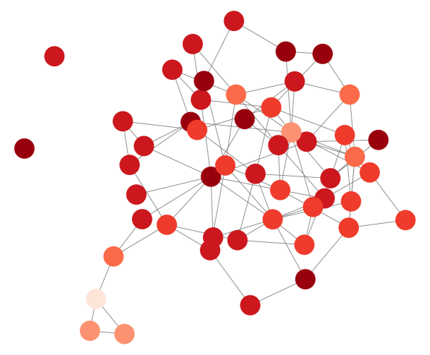
Figure 1: Graph of an adjacency matrix $A$ nodes and values of variable $y$, a simulated SAR model with one covariate

library(network)
library(RColorBrewer)
library(classInt)
library(GGally)
net1   = network(A, directed = FALSE)
net1$y = y
colors = brewer.pal(7, "Reds")
brks   = classIntervals(y, n=7, style="equal")
brks   = brks$brks #plot the map
ggnet2(net1,node.color=colors[findInterval(net1$y, brks,all.inside=TRUE)])

Once we have a data set and a model, we wish to estimate the model parameters. In this paper we use Hamiltonian Monte Carlo methods (HMC, see for example Neal (2011)), but you are free to choose your favorite MCMC method such as Gibbs sampling. To proceed with our example we need to load another library, the R Stan, to which our function solv.SAR is just a mask to help beginners. But if you wish to design a more complex model we encourage you to write your own codes using RStan. Because our function was designed mainly for didactic objectives it is limited to just two covariates and a number of chains between two and four.

n_samples  = 10000
prior      = c(0.01,0.01,100)
data_cov0  = list(N=n, y=z, W=W, prior=prior)
data_cov1  = list(N=n, y=z, W=W, x=as.matrix(x[,1]), prior=prior)
data_cov12 = list(N=n, y=z, W=W, x=x, prior=prior)
m0  = solv.SAR(data=data_cov0, ncov=0, nchain=2, n_iter=n_samples)
m1  = solv.SAR(data=data_cov1, ncov=1, nchain=2, n_iter=n_samples)
m12 = solv.SAR(data=data_cov12, ncov=2, nchain=2, n_iter=n_samples)
m1

The object $n\_samples$ is the number of samples of HMC, half of them will be discarded as burn-in. The vector $prior$ includes $a$, $b$ and $\sqrt{\eta}$ respectively. A warning here is that smaller values than 0.01 to $a$ or $b$ could produce computational problems later at the time to estimate any divergence, except to Kullback-Leiber divergence. The scalar $N$ is the length of $y$. With this information we build a list which is a prerequisite to solve the SAR model by Stan. Furthermore we require an additional information $ncov$ the number of covariates in the model and $nchain$ the number of chains desired, which must be between 2 and 4. Enter $m1$ to display a huge table with all posterior analysis of parameters and transform parameters. We summarize just the information on the main parameters in Table 1.

The chains for all parameters converged by $\hat{R}$ criterion (Gelman and Rubin (1992) and Brooks and Gelman (1998)). Yet another good result is the large values of effective sample sizes (ESS), around five thousand of samples to all estimations, which renders highly efficient estimates with small standard errors. Recall that the input values to each parameter were respectively zero to $\beta_{0}$, 0.3 to $beta_{1}$, 0.75 to $\rho$ and 1 to $\sigma$. You can see in Table 1 that the first two parameters were worstly estimated than the later two. Fortunately, $\rho$ and $\sigma$ are much more vital to the model.

Table 1: Summary of Posterior of SAR model parameters with one covariate.

parameter	Mean	2.5%	50%	97.5%	ESS	$\hat{R}$
$\beta_{0}$	-0.46	-1.07	-0.46	0.13	4823	1
$\beta_{1}$	-0.39	-0.82	-0.39	0.05	4862	1
$\rho$	0.75	0.49	0.75	0.97	4978	1
$\sigma$	2.05	1.39	1.99	3.02	5920	1

3 Comparison of models

An important step in any data analysis is to choose between a set of candidate models. To proceed with model comparison and selection we describe some statistical tools in the class of information criteria. Here we show two Bayesian criteria which generalize the well know Deviance Information Criterion (DIC), namely the Watanabe-Akaike Information Criterion (WAIC), designed by Watanabe (2010) and the leave-one-out cross-validate (LOO-CV) (see Vehtari et al. (2016)). The formulation of each criterion is expressed in equations 2 and 3, respectively.

$$WAIC=-2\sum_{i=1}^{n}\left(\log\dfrac{1}{S}\sum_{s=1}^{S}p(y_{i}|\boldsymbol{\theta}^{s})\right)+2\sum_{i=1}^{n}\left(Var_{s=1}^{S}\log p(y_{i}|\boldsymbol{\theta}^{s})\right).$$ (2)

$$\textit{LOO-CV}=-2\sum_{i=1}^{n}\left(\log\dfrac{1}{S}\sum_{s=1}^{S}p(y_{i}|\boldsymbol{\theta}^{is})\right)+\dfrac{2}{n}\sum_{i=1}^{n}\sum_{j=1}^{n}\left(\log\dfrac{1}{S}\sum_{s=1}^{S}p(y_{j}|\boldsymbol{\theta}^{is})\right).$$ (3)

Even if the mathematical formulas are extensive, they can be easily computed by loo package if the log likelihood function for transformed parameters in embeded in the Stan model. Again this is already implemented in our BDSAR package.

To be clear, the estimation of LOO-CV and WAIC is not performed by BDSAR, but by loo package. However we offer a fine plot which summarizes the results of loo as you can see from the example below. This is the function plot.loo which requires three components: n.mod the specification of how many models are under comparison, tab.loo a matrix with paste results from Leave one out, tab.waic an analog matrix to store WAIC values. Finally you can choose between color equal to TRUE or FALSE if you want a colorful plot or a black and white style. Figure 2 illustrates the first option. We remark that this function takes advantage of ggplot2 package resources.

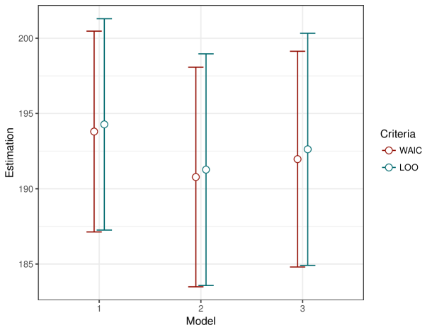
Figure 2: Comparison of three models by LOO and WAIC: M1 is a SAR without covariates, M2 is a SAR with one covariate, M3 is a SAR with two covariates.

log_lik0  = extract_log_lik(m0, parameter_name = "log_lik")
log_lik1  = extract_log_lik(m1, parameter_name = "log_lik")
log_lik12 = extract_log_lik(m12, parameter_name = "log_lik")
loo0      = loo(log_lik0)
loo1      = loo(log_lik1)
loo12     = loo(log_lik12)
waic0     = waic(log_lik0)
waic1     = waic(log_lik1)
waic12    = waic(log_lik12)
tab.loo   = matrix(cbind(loo0,loo1,loo12))
tab.waic  = matrix(cbind(waic0,waic1,waic12))
plot.loo(n.mod=3, tab.loo, tab.waic, color=TRUE)

We note in Figure 2 that the correct model (M2) has smaller WAIC as well as LOO. This point estimator indicates that both criteria work well for this kind of model, however the criteria standard errors are relatively large and hamper stronger conclusions. Unfortunately, this problem could not be solved by simply increasing the number of simulated samples of HMC.

4 Bregman Divergence

In this section we finally discuss about the core of BDSAR package, i.e. about Bregman divergence which is a way to measure distance between probability distributions. Consequently it could be used in diagnostic analysis, e.g. checking about influential observations.

The reader should be familiar with the Kullback-Leiber divergence, to which Bregman divergence is a generalization. We define $(X,\Omega,v)$ as a finite measure space and $f_{1}(x)$ and $f_{2}(x)$ as two non-negative functions where any probability density function is a special case of $f_{1}(x)$ or $f_{2}(x)$.

Let $\psi:(0,\infty)\rightarrow\mathbb{R}$ be a strictly convex and differentiable function. Then the functional Bregman divergence $D_{\psi}$ is defined as,

$$D_{\psi}(f_{1},f_{2})=\int\{\psi[f_{1}(x)]-\psi[f_{2}(x)]-[f_{1}(x)-f_{2}(x)]\psi^{\prime}[f_{2}(x)]\}dv(x),$$ (4)

where $\psi^{\prime}$ represents the derivative of $\psi$.

The choice of the convex function $\psi$ presents some degree of freedom. Here we follow the suggestion of Goh and Dey (2014) and restrict attention to the class of convex functions defined by Eguchi and Kano (2001), i.e. $\psi_{\alpha}(x)$, with $\alpha\in\mathbb{R}$.

$$\psi_{\alpha}(x)=\left\{\begin{matrix}(x^{2}-2x+1)/2,&\alpha=2\\ x\log x-x+1,&\alpha=1\\ -\log x+x-1,&\alpha=0\\ (x^{\alpha}-\alpha x+\alpha-1)/(\alpha^{2}-\alpha),&\mbox{otherwise}.\end{matrix}\right.$$ (5)

Following Goh and Dey (2014), we have a direct comparison if we take advantage of some simulation technique, as for example Importance-Weighted Marginal Density Estimation (IWMDE). These authors proposed this technique to Bayesian models with independent observations, comparing a vector $\mathbf{y}$ with $\mathbf{y}_{(i)}$, where the second vector is equal to the first but without the $i$-th observation, i.e. $\mathbf{y}_{(i)}=(y_{1},\dots,y_{i-1},y_{i+1},\dots,y_{n})$. We extend their results to correlated data using a strategy in which our second vector incorporates an imputation of the $i$-th observation, i.e. $\mathbf{y}_{(i)}=(y_{1},\dots,\hat{y}_{i},\dots,y_{n})$.

yhat   = y.hat(mod=m1,n=n,method=1)
draws  = as.matrix(m1)
theta  = as.matrix(cbind(draws[,3],draws[,4],draws[,1],draws[,2]))
kl     = KL.SAR(y=z,yhat=yhat,w=W,theta=theta,x=as.matrix(x[,1]),type=1)
is     = IS.SAR(y=z,yhat=yhat,w=W,theta=theta,x=as.matrix(x[,1]),prior=prior,
         dist=3,type=1)
breg   = BD.SAR(y=z,yhat=yhat,w=W,theta=theta,x=as.matrix(x[,1]),prior=prior,
         dist=3,alpha=2,type=1)
plot(kl,col=2,pch=2,ylab="D",xlab="obs")
plot(is,col=3,pch=8,ylab="D",xlab="obs")
plot(breg,col=4,pch=4,ylab="D",xlab="obs")

Here we show how to calculate the Bregman divergence as well as two famous specific cases: Kullback-Leiber and Itakura-Saito. First define a vector yhat which approximates $y$ using our function y.hat which requires a model, the length of $y$ and an imputation method which could be 1 for mean or 2 for median. The matrix $theta$ is just a compilation of parameter sampling by HMC; again we remark that the package does not require a specific MCMC scheme and you could use another sampling method. However $theta$ must be organized as $\rho$, $\sigma$, $\beta_{0},\beta_{1},\dots,\beta_{k}$ respectively. The option $dist$ corresponds to a distribution required by the IWMDE simulation technique. This takes values 1 for Exponential, 2 for Gamma, 3 for Normal or 4 for Multivariate Normal. According to Goh and Dey (2014) the success of the simulation depends of a accurate choice of this distribution, however there is no restriction to it. The parameter $\alpha$ takes on any real value, except 1 and 0, because this corresponds to Kullback-Leiber and Itakura-Saito, respectively.

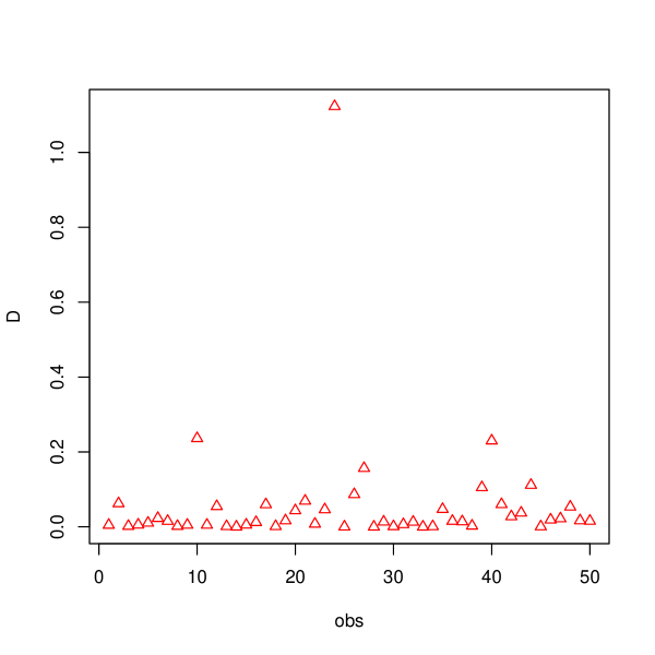
Figure 3: Kullback-Leiber divergence to each observation of $z$, a SAR process with one outlier

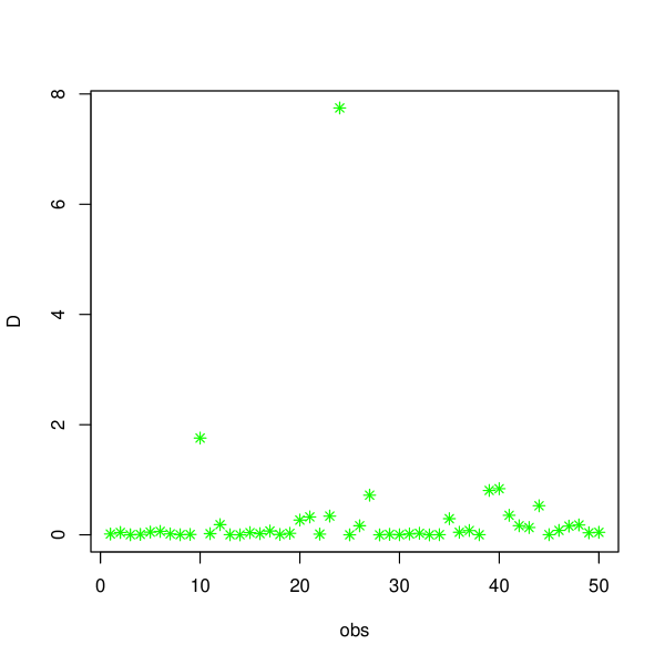
Figure 4: Itakura-Saito divergence to each observation of $z$, a SAR process with one outlier

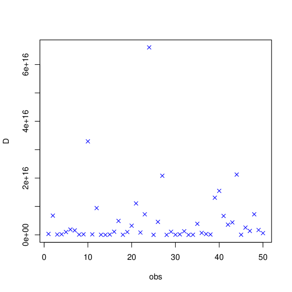
Figure 5: Bregman divergence with $\alpha=2$ to each observation of $z$, a SAR process with one outlier

In this paper we also propose an alternative way to compare the Bregman divergence between two points, which consists of looking at a proportion, $P_{i}$. Once the posterior is estimated and the matrix of simulated parameters is available it is easy to obtain a matrix $D$ with divergences, with $s$ rows from each Monte Carlo sampling and $i$ columns to each observation from the vector $y$. We then count how many times each observation from $y$ displays the supreme estimation of divergence along the MCMC iterations. Taking the mean of these counts we obtain a proportion, as shown in equation 6. This procedure is inspired in the work of Santos and Bolfarine (2016) and is obtained in the BDSAR package if the option type equal to 2 is selected.

$$P_{i}=\dfrac{1}{S}\sum_{s=1}^{S}\gamma_{s}\left\{\begin{array}[]{l}\gamma_{s}=1\text{ , if }\hat{D}^{s}_{i}=\sup\{\hat{D}^{s}\}\\ \gamma_{s}=0\text{ , otherwise. }\end{array}\right.$$ (6)

Our last example compares three divergence measures using the type 2 option, i.e. computing the proportions. The divergences are the same from the other example, K-L, I-S and L2/2, the Euclidean distance being a special case of Bregman when $\alpha$ is equal to 2. An obvious advantage of looking at the divergence as a proportion is that it scales to a number between zero and one instead of between zero and infinity. Consequently it becomes easier to compare divergences as depicted in Figure 6, where the three measures are presented. Note that there is an outlier in position 10, but by all divergences the position 24 is viewed as a more important influential point. The most famous of the three is the K-L, but this measure displays the observation 10 as the third most important, differently of the Euclidean distance which classifies the observation 10 as the second most relevant influence.

kl2   = KL.SAR(y=z,yhat=yhat,w=W,theta=theta,x=as.matrix(x[,1]),type=2)
is2   = IS.SAR(y=z,yhat=yhat,w=W,theta=theta,x=as.matrix(x[,1]),prior=prior,
        dist=3,type=2)
breg2 = BD.SAR(y=z,yhat=yhat,w=W,theta=theta,x=as.matrix(x[,1]),prior=prior,
        dist=3,alpha=2,type=2)
plot(c(1,n),c(0,1),ylab="P",xlab="obs",type="n")
lines(kl2,   col=2,pch=2,type="p")
lines(is2,   col=3,pch=8,type="p")
lines(breg2, col=4,pch=4,type="p")
legend("topright",col=c(2,3,4),pch=c(2,8,4),legend = c("K-L","I-S","L^2/2"))

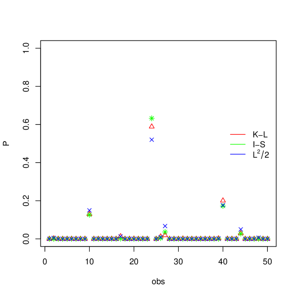
Figure 6: Comparison of three measures of divergences estimate by posterior probability to each observation of $z$, a SAR process with one outlier.

5 Conclusion

This paper offers a vignette structure which permits the reader to follow the point with continuous code. All the examples come from easily simulated data, so it can be reproduced by anyone. The sequence of arguments were organized as a full Bayesian analysis, i.e. estimate and compare models, as well as check of assumptions and influential observations by Bregman divergence. The BDSAR customize other packages to provide visual tools for analysis.

For the analysis of influential observations we extended the computation of Bregman divergence to spatially correlated data and proposed a reescaling to the interval (0,1) which facilitates comparisons. In our notation, $P_{i}$ corresponds to the posterior proportion of supreme cases by observation, i.e. the most atypical observations have more chance to present more frequently the supreme divergence.

Therefore, we believe in the relevance and usefulness of the package BDSAR and this paper as a useful guide to the main ideas.

6 Acknowledgement

Ian Danilevicz was supported by a scholarship from the Ministry of Education funding agency, CAPES. Ricardo Ehlers received support from São Paulo Research Foundation (FAPESP) - Brazil, under grant number 2016/21137-2

References

- Anselin (1988) Anselin, L. (1988). Spatial Econometrics: Methods and Models. Dordrecht: Kluwer Academic Publishers.
- Besag (1974) Besag, J. (1974). Spatial interaction and the analysis of lattice systems. Journal of the Royal Statistical Association, Series B, 36, 192–236.
- Brooks and Gelman (1998) Brooks, S. and Gelman, A. (1998). General methods for monitoring convergence of iterative simulations. Journal of Computational and Graphical Statistics, 7, 434.
- Cressie (1993) Cressie, N. (1993). Statistics for Spatial Data. Wiley, New York, revised edition.
- De Oliveira and Song (2008) De Oliveira, V. and Song, J. (2008). Bayesian analysis of simultaneous autoregressive models. Sankhyã: The Indian Journal of Statistics, Series B, 70(2), 323–350.
- Eguchi and Kano (2001) Eguchi, S. and Kano, Y. (2001). Robustifying maximum likelihood estimation. Institute of Statistical Mathematics. Technical Report, Tokyo Japan.
- Gelman and Rubin (1992) Gelman, A. and Rubin, D. B. (1992). Inference from iterative simulation using multiple sequences. Statistical Science, 7, 457–511.
- Goh and Dey (2014) Goh, G. and Dey, D. K. (2014). Bayesian model diagnostics using functional Bregman divergence. Journal of Multivariate Analysis, 124, 371–383.
- Lee and Nelder (1996) Lee, Y. and Nelder, J. (1996). Hierarchical generalized linear models (with discussion). Journal of the Royal Statistical Society, Series B, 58, 619–678.
- Neal (2011) Neal, R. M. (2011). MCMC using Hamiltonian dynamics. In Handbook of Markov chain Monte Carlo, pages 113–162. Boca Raton: Chapman and Hall-CRC Press.
- R Development Core Team (2015) R Development Core Team (2015). R: A language and environment for statistical computing. R Foundation for Statistical Computing, Vienna, Austria.
- Santos and Bolfarine (2016) Santos, B. and Bolfarine, H. (2016). On Bayesian quantile regression and outliers. ArXiv e-prints.
- Vehtari et al. (2016) Vehtari, A., Gelman, A., and Gabry, J. (2016). Practical Bayesian model evaluation using leave-one-out cross-validation and WAIC. Statistics and Computing.
- Watanabe (2010) Watanabe, S. (2010). Asymptotic equivalence of Bayes cross validation and widely applicable information criterion in singular learning theory. Journal of Machine Learning Research, 11, 3571–3594.