Influence of parameterized small-scale gravity waves on the migrating diurnal tide in Earth’s thermosphere

Abstract

Effects of subgrid-scale gravity waves (GWs) on the diurnal migrating tides are investigated from the mesosphere to the upper thermosphere for September equinox conditions, using a general circulation model coupled with the extended spectral nonlinear GW parameterization of Yiğit et al. (2008). Simulations with GW effects cut-off above the turbopause and included in the entire thermosphere have been conducted. GWs appreciably impact the mean circulation and cool the thermosphere down by up to 12-18%. GWs significantly affect the winds modulated by the diurnal migrating tide, in particular in the low-latitude mesosphere and lower thermosphere and in the high-latitude thermosphere. These effects depend on the mutual correlation of the diurnal phases of the GW forcing and tides: GWs can either enhance or reduce the tidal amplitude. In the low-latitude MLT, the correlation between the direction of the deposited GW momentum and the tidal phase is positive due to propagation of a broad spectrum of GW harmonics through the alternating winds. In the Northern Hemisphere high-latitude thermosphere, GWs act against the tide due to an anti-correlation of tidal wind and GW momentum, while in the Southern high-latitudes they weakly enhance the tidal amplitude via a combination of a partial correlation of phases and GW-induced changes of the circulation. The variable nature of GW effects on the thermal tide can be captured in GCMs provided that a GW parameterization (1) considers a broad spectrum of harmonics, (2) properly describes their propagation, and (3) correctly accounts for the physics of wave breaking/saturation.

1. Introduction

Vertically propagating internal gravity waves (GWs) of lower atmospheric origin significantly affect the dynamics of the middle atmosphere, where their role is widely appreciated (e.g., see the review of Fritts and Alexander, 2003). Studies over the last decade demonstrated that these waves can effectively propagate deep into the thermosphere despite the steeply growing molecular diffusion and thermal conduction (Yiğit et al., 2008; Hickey et al., 2009, 2010; Fritts and Lund, 2011; Gavrilov and Kshevetskii, 2013; Vadas and Fritts, 2005; Vadas et al., 2014; Heale et al., 2014), and considerably influence the state and circulation at altitudes up to the F region of the ionosphere (Yiğit et al., 2009; Miyoshi et al., 2014). The most recent review of these studies can be found in the works of Yiğit and Medvedev (2015); Yiğit et al. (2016) and in the book by Yiğit (Chapter 5, 2015). In addition to the dynamical forcing, GWs contribute to heating and cooling of the thermosphere above the turbopause ($\sim$105 km) up to F₂ layer altitudes, reaching peak values of $\sim 170$ K day^-1 (Yiğit and Medvedev, 2009). Since the thermosphere is strongly susceptible to variations of solar activity, GW propagation and effects exhibit appreciable changes, as was predicted by general circulation models (GCMs) (Yiğit and Medvedev, 2010) and recently demonstrated by satellite observations (Park et al., 2014; Garcia et al., 2016). Transient events in the lower and middle atmosphere, such as sudden stratospheric warmings, also alter propagation of GWs causing an increase of the GW activity in the upper thermosphere by more than a factor of three (Yiğit and Medvedev, 2012, 2016) and generating changes in the thermospheric circulation up to $\pm 50\%$ (Yiğit et al., 2014). Obviously, in order to achieve a physically consistent picture of middle and upper atmospheric dynamics, GW effects cannot be ignored, and any GCM extending to thermospheric heights must properly account for their effects.

Thermal tides are persistent large-scale atmospheric oscillations of the field variables (temperature, wind, pressure, density) that are generated at various altitudes within the atmosphere. They are produced by periodic heating due to absorption of incoming solar radiation (Siebert, 1961). In the lower atmosphere, they are generated by the absorption of UV radiation by stratospheric ozone and of IR by tropospheric water vapor (Forbes, 1984), and by latent heat release (Hagan and Forbes, 2002, 2003). Thermospheric migrating tide is excited in situ primarily by photoabsorption of solar radiation in the UV and EUV wavelength range by molecular oxygen (Fesen et al., 1986).

The diurnal westward propagating tide with the zonal wavenumber one (DW1) is a prominent mode in the mesosphere and the lower thermosphere (MLT) (Lieberman and Hayes, 1994). The diurnal amplitudes in the zonal and meridional wind components demonstrate a distinct semiannual cycle, and reach maxima during equinoxes (Hays et al., 1994; Manson et al., 2002a, b; Wu et al., 2006; Lieberman et al., 2010) and minima during solstices (Pancheva et al., 2002; Davis et al., 2013).

In the thermosphere, thermal tides emanating from below are supplemented by in-situ generated solar tides (Hagan et al., 2001), which are especially strongly excited in low-latitudes (Forbes et al., 1993). Characterization of tidal signatures of lower atmospheric origin in the atmosphere above turbopause altitudes and quantification of their dynamical effects on the thermospheric temperature and mean flow are crucial for better understanding the degree of vertical coupling (Pancheva et al., 2006; Knížová et al., 2015). Since the advent of global satellite observations, propagation of tidal signatures into the thermosphere have been increasingly studied (e.g., Huang and Reber, 2003; Oberheide et al., 2011; Pancheva et al., 2012; Pancheva and Mukhtarov, 2012; Häusler et al., 2015). With only a few months of measurements, satellites can provide good local time and longitudinal coverage. Analyzing neutral density measurements by accelerometers onboard the CHAMP (Challenging Minisatellite Payload) and GRACE (Gravity Recovery and Climate Experiment) satellites, Forbes et al. (2009) showed that tides originating in the troposphere have a significant impact on the MLT, and that the tidal influences can extend up to the exosphere linking exospheric variability to the variability near the surface.

Interactions of GWs and thermal tides have been a subject of numerous studies (e.g., Miyahara and Forbes, 1991; Manson et al., 1998, 2002c, 2002a, 2004; Achatz et al., 2008; Chang et al., 2008; Watanabe and Miyahara, 2009; Beldon and Mitchell, 2010; Senf and Achatz, 2010; Liu et al., 2013; Heale and Snively, 2015). The majority of these studies focused on the MLT region, while the influence of GWs on tides in the upper thermosphere received little attention or no attention at all. Partially, this was caused by a relative scarcity of observations and by inability of GW parameterizations, which were developed primarily for middle atmosphere models, to capture GW propagation and effects in whole atmosphere GCMs above the turbopause. Our study addresses this gap in the knowledge by considering GW effects on the diurnal migrating tides at altitudes from the tropopause ($\sim$15 km) to the upper thermosphere ($\sim$300 km), corresponding to the ionospheric F₂ layer altitudes.

How do upward propagating thermal tides, in-situ generated thermospheric tides and GWs interact within the context of vertical coupling? What are the implications of GW penetration into the upper atmosphere for the tidal wave structures? What is needed for GCMs to realistically capture GW-tide interactions? These questions were the essential motivation for this paper. Given that internal GWs and tides both grow in amplitude with height, and that they largely dissipate in the middle and upper atmosphere, interactions of these waves play a substantial role in the energy and momentum budget in these regions. Various aspects of GW-tidal interactions have been studied in a number of publications. Using a numerical model of the diurnal tide coupled with simplified linear GW drag calculations, Miyahara and Forbes (1991) showed, considering only harmonics with slow horizontal phase speeds, that GW stress reduces the tidal amplitudes in the MLT. With a linear steady-state tidal model complemented by a linear GW parameterization, Meyer (1999) examined the role of GW effects in the seasonal variations of the diurnal tides. Observations of the diurnal tide amplitude and phase variability with the medium frequency and meteor radars in the MLT revealed a modulation of GW propagation and momentum fluxes by tides (Nakamura et al., 1997). The study of Manson et al. (2002c) showed that the tidal winds simulated by a GCM strongly depend on the utilized GW parameterization. In addition to modeling, interactions between GWs and tides have been studied with observations (e.g., Manson et al., 1998; Beldon and Mitchell, 2010; Liu et al., 2013; Agner and Liu, 2015).

In this paper we re-examine the influence of upward propagating small-scale GWs on the migrating diurnal tide at altitudes from the middle atmosphere to the upper thermosphere. We consider the DW1 component because it dominates in the thermosphere, and focus on the September equinox, when tidal amplitudes are largest. We employ the CMAT2 (Coupled Middle Atmosphere Thermosphere-2) GCM with the implemented state-of-the-art nonlinear spectral GW parameterization of Yiğit et al. (2008), Global Scale Wave Model ((GSWM), Hagan and Forbes, 2003) tidal fields and NCEP (National Centers for Environmental Predictions) reanalysis data at 15 km.

The structure of the paper is as follows. Section 2 summarizes the main features of the CMAT2 GCM, the extended nonlinear GW parameterization of Yiğit et al. (2008), and the setup of the simulations. Sections 3 and 4 describe the modeled mean fields and mean GW effects during the September equinox, respectively. Simulations of the diurnal migrating tides are presented in section 5; diurnal variations of GW effects are analyzed in section 6. Longitudinal variations are investigated in section 7. Section 8 discusses our results in the context of the MLT and upper thermospheric dynamics. Summary and conclusions are given in section 9.

2. Model Description, Gravity Wave Scheme, and Experiment Design

Table 1Test runs used in the paper. In the cutoff simulation, EXP0, lower atmospheric GWs are not allowed to propagate into the thermosphere above $\sim$105 km, while in the extended simulation, EXP1, GWs propagate into the upper thermosphere.

Model Experiment	Experiment description
Cutoff Simulation (EXP0)	Gravity wave effects excluded above 105 km
Extended Simulation (EXP1)	Gravity wave effects included in the whole atmosphere

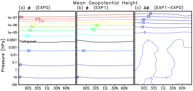
Figure 1.— Pressure-latitude distribution of the mean geopotential height [km] in (a) cutoff (EXP0) and (b) extended (EXP1) simulation. The difference field (EXP1-EXP0) is shown in (c).

The CMAT2 GCM is a three-dimensional general circulation model that extends from the tropopause ($\sim$15 km, 100 hPa) to the thermosphere to $\sim 250-500$ km ($1.43\times 10^{-8}$ hPa) depending on the solar and geomagnetic activity. It is a finite difference model that solves the energy, momentum, and mass conservation equations on a $18^{\circ}\times 2^{\circ}$ longitude-latitude grid at 63 fixed pressure levels. At the lower boundary, the model is forced by the National Centers for Environmental Prediction (NCEP) data, and the solar tides are specified at the lower boundary from the output of Global Scale Wave Model ((GSWM), Hagan and Forbes, 2003). The SOLAR2000 empirical model of Tobiska et al. (2000) is used in order for calculating thermospheric heating, photodissociation, and photoionization due to absorption of solar X rays, EUV and UV radiation between wavelengths 1.8 and 184 nm.

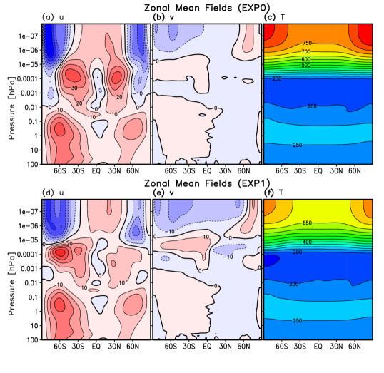
Figure 2.— Mean zonal mean atmospheric fields around September equinox for the zonal winds $u$, meridional winds $v$, and temperature $T$ from the left to right columns, respectively, simulated in the cut-off, i.e., EXP0, (panels a–c, top row) and extended, i.e., EXP1, (panels d–f, bottom row) gravity wave simulations. In the zonal wind and meridional wind plots, positive values (red shading, solid contour lines) represent eastward and northward winds, respectively. The contour intervals are 10 m s^-1 for winds 50 K for the temperature.

The model has a conventional (coarse-grid) resolution and cannot self-consistently simulate small-scale GWs. Therefore, the influence of subgrid-scale GWs on the large-scale circulation is represented by the extended spectral nonlinear GW parameterization (Yiğit et al., 2008). The development of this scheme has been reviewed in the work by Yiğit and Medvedev (2013). Various assumptions and limitations of GW parameterizations are discussed in detail in the review of Yiğit and Medvedev (2016). This scheme accounts for propagation and dissipation of GWs in the whole atmosphere due to nonlinearity ($\beta_{non}$) (Medvedev and Klaassen, 1995, 2000), molecular diffusion and thermal conduction ($\beta_{mol}$), eddy viscosity ($\beta_{eddy}$), ion drag ($\beta_{ion}$), and radiative damping ($\beta_{rad}$) in form of Newtonian cooling, which are calculated for each harmonic $i$ in a broad spectrum of gravity waves ($M=30$). Thus the total dissipation $\beta_{tot}^{i}$ for a given harmonic is given by

$$\beta_{tot}^{i}=\sum_{n}\beta_{n}^{i}=\beta_{non}^{i}+\beta_{mol}^{i}+\beta_{eddy}^{i}+\beta_{ion}^{i}+\beta_{rad}^{i},$$ (1)

where $n$ denotes the different dissipation terms listed above. The two major input parameters are the GW source spectrum, which specifies a distribution of GW activity in terms of horizontal momentum fluxes $\overline{u^{\prime}w^{\prime}_{i}}$ as a function of the horizontal phase speed $c_{i}$ at the lower boundary ($\sim$15 km) (Yiğit et al., 2012, Figure 1), where the subscript $i$ denotes a GW harmonic from the spectrum, and the horizontal wave number $k_{H}=2\pi/\lambda_{H}$. The assumed spectrum is in a qualitative and quantitative agreement with balloon measurements of GW activity (Hertzog et al., 2008, Figure 6). We assume the characteristic scale of $\lambda_{H}=300$ km, which is typical for lower atmospheric GWs to be parameterized (Samson et al., 1990). The GW harmonics are launched in the direction of the local wind at the lower boundary followed by evaluation of vertical profiles of the momentum fluxes at each grid point in the model. Although a fixed spectral shape of gravity wave distribution is assumed at the source, the actual GW source activity is highly variable as the source winds are spatiotemporally variable. The dynamical and thermal effects resulting from the divergences of the momentum fluxes are calculated as described in the works by Yiğit et al. (2009) and Yiğit and Medvedev (2009) and interactively applied to the simulated (large-scale) fields. The dynamical effects include the zonal ($a_{x}$) and meridional ($a_{y}$) GW drag given by

$$a_{x}=-\frac{1}{\rho}\frac{\partial(\rho\overline{u^{\prime}w^{\prime}})}{\partial x},\qquad a_{y}=-\frac{1}{\rho}\frac{\partial(\rho\overline{v^{\prime}w^{\prime}})}{\partial y},$$ (2)

where $\rho$ is the background neutral density. The thermal effects $Q$ incorporate the total resulting effects from irreversible heating $Q_{irr}$ and differential heating/cooling $Q_{dif}$ (Yiğit and Medvedev, 2009, Eqn. 1).

Figure 3.— Mean atmospheric difference fields obtained by subtracting the cutoff simulation results from the extended simulation (EXP1-EXP0).

The extended scheme has been validated in the works by Yiğit et al. (2009) and Yiğit and Medvedev (2009) with respect to MSIS and HWM (Horizontal Wind Model), two established empirical models of the thermosphere. The scheme was numerously applied in studies of atmospheric dynamics (Yiğit et al., 2009, 2012, 2014; Yiğit and Medvedev, 2009, 2010, 2012). It is also being used for Martian GCMs (Medvedev et al., 2011a, b, 2013, 2015, 2016; Medvedev and Yiğit, 2012; Yiğit et al., 2015a, b), and has been most recently successfully applied for interpretation of MAVEN (Mars Atmosphere Volatile EvolutioN) observations of high-altitude GWs in the thermosphere of Mars (Yiğit et al., 2015b).

The model is run for low solar and geomagnetic activity conditions ($F_{10.7}$ = 80 W m^-2 Hz^-1, $K_{p}$ = 2+) for about a half year, and data are output for every four hours around the September equinox over the period 19–25 September (i.e., about one week centered around the Northern Hemisphere autumnal equinox). This excludes the well known influence of high solar activity on GWs (Yiğit and Medvedev, 2010; Laskar et al, 2015) and larger-scale circulation (including in-situ excited tides) in the thermosphere, but still captures the mechanism of GW influence on the tides, which is of interest here. September zonal mean fields have been validated with respect to the HWM previously (Yiğit et al., 2012). In this study, in order to quantify GW effects on the migrating diurnal tide, we use simulation data produced by running the model in two modes: (1) with out and (2) with GW propagation into the thermosphere above the turbopause ($\sim$105 km), referred to as the “cutoff” (EXP0) and the “extended” (EXP1) simulations, respectively, as summarized in Table 1.

In practical terms, the notions of “cutoff” and “extended” simulations refer to the methodologies of excluding and including, respectively, the thermospheric effects of gravity waves of lower atmospheric origin, as calculated by the extended nonlinear GW parameterization (Yiğit et al., 2008). By default, this scheme calculates GW effects in the entire atmosphere, which corresponds to the “extended” case (“EXP1”) of the GCM simulation. In order to assess the significance GW propagation into the thermosphere, we additionally perform the cutoff simulation, which is designed to incorporate GW effects calculated by the GW scheme only from the lower atmosphere up to the turbopause.

In both cases, the GW effects are analyzed, and the modeled zonal ($u$) and meridional winds ($v$) as well as neutral temperature ($T$) fields are Fourier decomposed in order to obtain diurnal migrating tide amplitudes. We compare the cutoff and the extended simulation results at fixed pressure levels.

To provide a further perspective on the thermospheric extension of the model levels, we plotted the zonal mean geopotential height $Z_{\Phi}$ (in km) averaged over the chosen time interval in the entire model domain in Figure 1 for (a) EXP0 (cutoff), (b) EXP1 (extended), and (c) the difference between the extended and the cutoff simulations, i.e., EXP1–EXP0. Overall, the model covers altitudes from $Z_{\Phi}=15$ km to about 300 km under the assumed low solar and geomagnetic conditions. The turbopause reference height of $\sim$105 km is close to the $10^{-4}$ hPa pressure level and varies little between the two simulations. It is seen from Figure 1c that, below the turbopause, geopotential heights are nearly identical in both runs for all model pressure levels. Above it, accounting for the thermospheric effects of GWs leads to contraction of the thermosphere, i.e., thermospheric layer thickness reduces, and to drop of the geopotential heights of the fixed pressure levels relative to the cutoff simulation. The difference $\Delta Z_{\Phi}$ at fixed pressure levels due to GW effects vary from –5 km in the lower thermosphere to –30 km in the upper thermosphere.

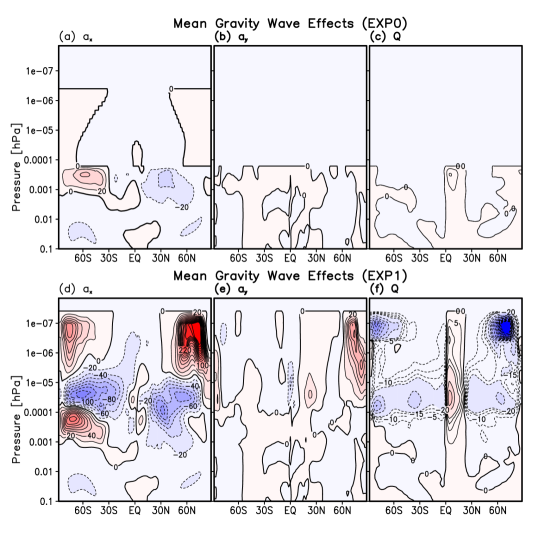
Figure 4.— Same as Figure 2 but for the GW dynamical ($a_{x},a_{y}$; acceleration/deceleration) and $Q$; thermal (heating/cooling) effects in m s^-1 day^-1 and K day^-1, respectively. Contour intervals are 20 m s^-1 day^-1 and 20 K day^-1. For $Q$, $\pm 5,\pm 10,and\pm 15$ K day^-1 contours have been added.

3. Zonal Mean Fields

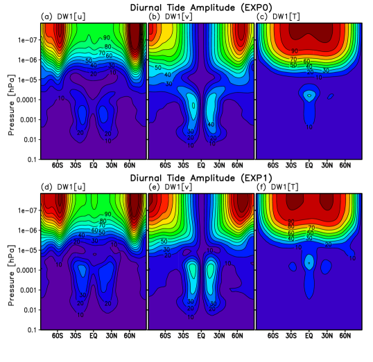
Figure 5.— Altitude (pressure)-latitude distributions of the amplitude of the diurnal migrating tide (DW1) for the zonal wind [m s^-1], meridional wind [m s^-1], and temperature [K] shown from left to right in the cut-off (panels a–c) and the extended (panels d–f) simulations.

We first analyze the altitude-latitude cross-sections of the zonal mean fields for the September equinox and the corresponding differences between the extended and the cutoff simulations. The columns from left to right in Figure 2 present the simulated mean zonal wind ($\bar{u}$), meridional wind ($\bar{v}$), and neutral temperature ($\bar{T}$), correspondingly, for the cutoff (EXP0, top row) and extended (EXP1, bottom row) runs. Red shading and solid lines denote westerly (eastward) winds, while blue shading and dashed lines are for easterly winds (westward) in units of m s^-1.

During the equinox, westerly zonal winds are predominant in the lower and middle atmosphere and are relatively weak (peak values are up to 40 m s^-1). Their extension into the upper thermosphere is modified primarily by Coriolis force, ion drag and high-latitude energy sources (e.g., Joule heating and particle precipitation) in addition to the rapidly increasing molecular diffusion. The equinoctial meridional circulation is also relatively weak (compared to the solstitial one), and the mean neutral temperature increases up to $\sim$750–900 K in the upper thermosphere.

Closer inspection of the mean fields reveals the major differences above 100 km between the two simulations, in particular for the zonal mean wind at middle- and high-latitudes, which we consider in detail in Figure 3 by evaluating the corresponding differences $\Delta\bar{u}$, $\Delta\bar{v}$, and $\Delta\bar{T}$ at fixed pressure levels. It is seen that accounting for GWs in the whole atmosphere provides more westerly (positive, red) momentum to the zonal wind in the high-latitude thermosphere, and more easterly momentum (blue shaded) in the middle-latitude thermosphere in both hemispheres. The strongest attenuation of the easterly wind takes place in the high-latitude F₂ region altitudes of the Northern Hemisphere (panel a). It leads to a weakening of the poleward meridional circulation in both hemispheres (panel b). One (already mentioned) remarkable thermal effect of GWs is cooling the lower thermosphere down by about 70 K ($18\%$) at low- and middle-latitudes. In the upper thermosphere, the temperature difference is even larger (80–90 K colder), although somewhat smaller in relative units: $>12-14\%$. These GW-induced changes in the background conditions should be kept in mind when analyzing vertical propagation of GWs and the tide.

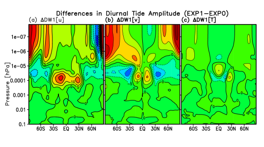
Figure 6.— Differences in the diurnal tidal (DW1) amplitudes of $u$, $v$, and $T$ between the extended and the cutoff simulations, i.e., EXP1-EXP0. Solid/dashed contours represent positive/negative differences. The contour intervals are 5 m s^-1 for the winds and 5 K for temperature.

4. Zonal Mean Gravity Wave Effects

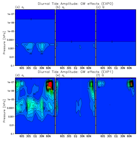
Figure 7.— Diurnal tidal amplitudes as in Figure 5 but for the GW zonal drag $a_{x}$, meridional drag $a_{y}$, and the total heating/cooling $Q$. The controur intervals are 30 m s^-1 day^-1 for drag and 30 K for heating/cooling.

The only systematic difference between the two simulations, EXP0 and EXP1, is the inclusion of the parameterized GW effects above $\sim$105 km. The parameterization scheme allows for quantifying these effects in order to gain further insight into the nature of changes in the modeled mean fields. Figure 4 presents the zonal mean ($\bar{a}_{x}$, panels a,d) and meridional ($\bar{a}_{y}$, panels b,e) GW forcing (“GW drag”) and the total GW-induced heating/cooling rates ($\bar{Q}$, panels c,f) for both simulations in a manner similar to that in Figure 2. The cutoff simulation illustrates the GW effects in the MLT on the mean zonal circulation: a weak westward drag of around –20 m s^-1 day^-1 in the stratosphere and +60 and –40 m s^-1 day^-1 in the MLT of the Southern and Northern Hemispheres, respectively. GWs impose a negligible mean meridional forcing and heating/cooling in the middle atmosphere. However, when GWs are allowed to propagate in the simulations beyond the turbopause, they produce substantial dynamical effects, primarily the eastward zonal GW drag in the lower and upper thermosphere and westward GW drag of more than –120 m s^-1 day^-1 in the middle-latitude middle thermosphere. Note also that GW drag increases in magnitude in EXP1 even below 105 km as a consequence of the downward control. The latter example emphasizes the importance of a correct accounting for GW physics in the thermosphere even if the area of interest is the MLT only.

The zonally averaged meridional GW forcing of $\sim\pm 20$ m s^-1 day^-1 around the equatorial lower thermosphere and 80 m s^-1 day^-1 in the high-latitude Northern thermosphere is expectedly smaller than that in the zonal direction. In the lower thermosphere, GWs provide cooling at middle- and high-latitudes ($\sim-40$ K day^-1) and heating in a narrow latitude band near the equator with 60 K day^-1. The thermal effects in the upper thermosphere are much larger. They include an intensive cooling at high-latitudes exceeding –100 K day^-1 and $\sim-260$ K day^-1 in the Southern and Northern Hemispheres, respectively. One may notice a certain degree of symmetry of GW-induced effects with respect to the equator during the equinox, although there are some noticeable interhemispheric differences in the magnitude of the effects due the interplay of background atmospheric wave filtering and dissipation.

The GW-induced differences in the simulated mean fields presented in Figure 3 can now be interpreted better together with the GW dynamical and thermal effects explicitly shown in Figure 4. Although the distributions of GW forcing and the induced changes generally agree, they do not fully coincide. This phenomenon illustrates that atmospheric dynamics is strongly nonlinear, interactions of GWs with the mean flow should not be viewed overly simplistic, and that employed GW parameterizations must capture the interactions with the larger-scale atmosphere, i.e., be physically based rather than mechanistic.

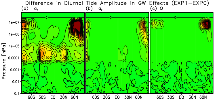
Figure 8.— Difference between the extended and the cutoff simulations in the diurnal tidal amplitudes for $a_{x},a_{y}$, and $Q$. The controur intervals are 30 m s^-1 day^-1 for drag and 30 K for heating/cooling.

5. Diurnal Migrating Solar Tide

Model simulations considered above demonstrated that propagation and dissipation of GWs in the thermosphere above the turbopause result in significant changes in the general circulation and mean thermal structure of the atmosphere. This finding brings in the main question of this paper: To what extent do GW effects impact the diurnal tide in the middle and upper atmosphere? For this, we next consider the tidal fields in winds and neutral temperature. They represent composites over the model 19-25 September and, thus, offset a day-to-day tidal variability (Liu, 2014).

Figure 5 shows the diurnal tide amplitudes for the same components ($u$, $v$, and $T$) as the mean fields presented in Figure 2 for the both runs. There are two disparate maxima. The first one is in the low-latitude MLT, and is created by the tides generated in the lower atmosphere and propagating upward. The much larger (velocity amplitudes are more than 150 m s^-1) maximum in the upper thermosphere (above $\sim$150 km) is due to the tide generated in-situ by absorption of solar EUV radiation and ion-neutral coupling (Fesen et al., 1986). The structure and amplitude of the diurnal migrating tide in the MLT are well documented with observations (e.g., McLandress et al., 1996; Manson et al., 2002b; Wu et al., 2006; Lieberman et al., 2010; Agner and Liu, 2015). The simulated morphologies of the tidal amplitudes in the MLT are in a good qualitative agreement with previous observations. Namely, the amplitudes of the zonal and meridional wind components peak around 20^∘N and $20^{\circ}$S at around 100 km with the amplitude of meridional wind variations exceeding that for the zonal component, and have a distinctive “butterfly” pattern consistent with the TIDI (TIMED Doppler Interferometer) measurements (Wu et al., 2006, 2008). The amplitude of temperature tidal perturbations has the maximum (15-20 K) over the equator in the MLT, and at low-latitudes in the upper thermosphere ($\sim$100 K).

There are some differences in the magnitude and structure of the tide between the two simulations. They are plotted in Figure 6. Substantial differences in the amplitudes of the zonal and meridional winds are seen above the turbopause and, to a minor extent, in the MLT. GW-induced changes in the temperature component of the diurnal tide amplitude are mainly confined to the equatorial region of the MLT. Accounting for GW effects in the simulations changes diurnal fluctuations of temperature by $\pm$10 K in the lower thermosphere, or up to 30% of the tide amplitude. For the zonal and meridional winds, GWs facilitate an increase of tidal amplitudes in the low-latitude MLT, and decrease them at higher latitudes slightly higher (around 120–140 km). The amplitude of zonal wind tidal oscillations increases by up to 20 m s^-1 between $\pm 30^{\circ}$ and decreases by up to $10$ m s^-1 poleward of $\pm 45^{\circ}$.

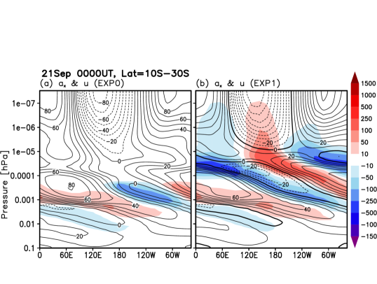
Figure 9.— Pressure-longitude distribution of Southern Hemisphere low-latitude average ($10^{\circ}-30^{\circ}$S) of the zonal wind (contour) [m s^-1] and zonal GW drag (shaded) [m s^-1 day^-1] at a representative universal time (0000 UT) on 21 Sept 0000 UT in the cutoff (EXP0) and the extended simulation (EXP1). The zonal wind contour intervals are 10 m s^-1.

In the thermosphere above $\sim$150 km, the inclusion of parameterized GW effects resulted in the tidal wind amplitudes increase by up to 25 m s^-1, with the exception of zonal winds at high latitudes of the Northern Hemisphere. There, the amplitudes decreased by up to $\sim$–20 m s^-1. The tidal amplitude change in temperature is $\sim$5 K in the high-latitudes, and about $10$ K in the low-latitudes. Overall, the simulations show where and how GWs impact the diurnal tide most significantly. In the horizontal wind fields, the effect of the parameterized GWs occurs nearly at all latitudes in the MLT and, predominantly, at middle- and high-latitudes in the upper thermosphere, where tidal variations of wind are largest. Similarly, the temperature component of the diurnal tide is affected, primarily, in the equatorial thermosphere, where the diurnal temperature fluctuations are large.

We next embark on further details of how GWs can produce the changes in amplitude and structure of the DW1 tide by analyzing diurnal variations of the GW drag. Previous studies that were concerned mainly with the MLT have indicated that the effects of parameterized GWs depend on the relative phase between the GW forcing and the tides (Liu et al., 2013).

6. Diurnal Variation of Gravity Wave Effects

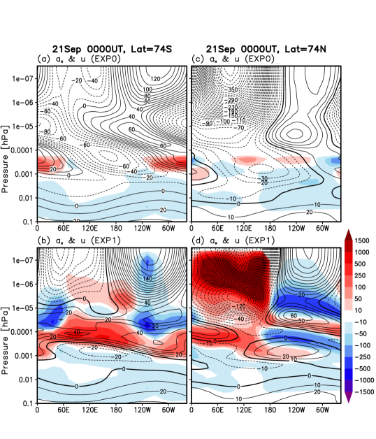
Figure 10.— Same as Figure 9 but for the Southern Hemisphere ($74^{\circ}$S) and Northern Hemisphere ($74^{\circ}$N) high-latitudes.

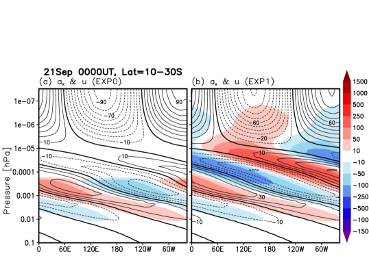
Figure 11.— Diurnal component of the zonal wind and the zonal GW drag presented in Figure 9 at the Southern Hemisphere low-latitudes on 21 Sept 0000 UT.

We next investigate diurnal variations of GW effects. Figure 7 presents the diurnal tidal amplitudes of zonal GW drag, meridional GW drag, and the total GW heating/cooling rate, for the cut-off and extended simulations, presented in a similar way as in the preceeding figures. Overall, the largest diurnal variations are seen in the zonal GW drag. In the cut-off simulation, these variations are confined to the low-latitude MLT with peak values of $\sim$90 m s^-1 day^-1 centered around $\sim$$\pm 30^{\circ}$ latitude. The meridional GW drag and GW heating/cooling rates show very weak diurnal variations. In the extended simulation, GW diurnal variations are more remarkable in all GW parameters. The peak values of the zonal GW drag variations are situated around the low-latitude MLT, have a similar structure as in the cut-off simulation, but much stronger amplitude of up to 210 m s^-1 day^-1, extending to higher altitudes in the thermosphere. Overall, some degree of hemispheric asymmetry is seen in the diurnal tidal signature in the zonal GW drag.

At higher levels in the thermosphere, the zonal GW drag demonstrates prominent diurnal variations at high-latitudes with peak values of $\sim$200 m s^-1 day^-1 in the Southern Hemisphere and several hundred m s^-1 day^-1 in the Northern high-latitudes. The maximum of diurnal variations of the meridional GW drag and total GW heating/cooling peak in the high-latitudes thermosphere of the Northern Hemisphere.

Analyzing the difference in the GW diurnal variations in Figure 8 between the cutoff and the extended simulations demonstrates that the GW diurnal variations are large in the extended simulation in all regions. This suggests that GW propagation into the thermosphere is strongly modulated by the diurnal tide, and that GW-tide interactions and nonlinear feedback would not be captured if GWs are not accounted for in the whole atmosphere system. The diurnal tidal variations in the MLT extend higher up in the lower thermosphere in the extended simulation. It is noteworthy that the lower thermospheric GW effects produce changes below the turbopause, as indicated by the nonzero difference in the diurnal tidal amplitude in $a_{x}$ (panel a). The simulations also highlight that the zonal GW drag experiences significant diurnal variations in the lower thermosphere above the turbopause. Comparison of differences in the diurnal tidal amplitudes in the fields (Figure 6) with the differences in the diurnal amplitudes of GW effects (Figure 8) provides further insight into interactions of GWs and tides. In the low-latitude lower thermosphere at around $\pm 30^{\circ}$, the enhancement of the GW diurnal amplitude coincides very well with the enhancement of tidal variations, in particular, of the zonal wind, when GW effects are included in the whole atmosphere. In the upper thermosphere, strongest diurnal variations of the GW drag occur in the regions where either the enhancement of diurnal oscillations of wind takes place, i.e., in the high-latitude Southern Hemisphere, or the amplitude is strongly reduced (in the high-latitude Northern Hemisphere). We next focus on these regions where largest diurnal variations of GW effects lead opposite consequences for the tidal amplitudes.

7. Longitudinal Variations

Next, we assess the altitude-longitude distributions of the zonal winds and zonal component of GW drag during the September equinox at a representative universal time (00:00 UT) in order to gain further insight into GW-tidal interactions. Figure 9 presents the Southern Hemisphere zonal wind fields (contour) and the zonal GW drag (color shades) for the cutoff (EXP0, top panel) and the extended (EXP1, bottom panel) simulations averaged over low-latitudes 10${}^{\circ}-30^{\circ}$S. It is seen that, in the low-latitude MLT, the directions of the GW drag and the wind remarkably coincide, that is, GWs accelerate the local winds rather than “drag” them. In the EXP1 simulation, this directional correlation of the wind and GW forcing extends higher into the thermosphere up to $10^{-5}$ hPa ($\sim$140 km). Further above this height, the in-situ generated tide takes over the one propagating from below, and the effect of GWs changes accordingly – GWs act to weakly decelerate the zonal flow in the middle and upper thermosphere at low-latitudes.

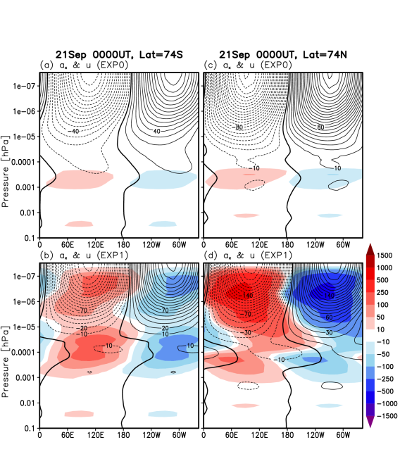
Figure 12.— Diurnal component of the zonal wind and the zonal GW drag presented in Figure 10 at Southern (left) and Northern (right) Hemisphere high-latitudes on 21 Sept 0000 UT.

At high-latitudes, thermospheric GW effects are more variable owing to additional energy and momentum sources of magnetospheric origin that modulate the background atmosphere. Figure 10 presents the results of simulations for the Southern ($74^{\circ}$S) and Northern Hemisphere ($74^{\circ}$N) high-latitudes. The varying depth of GW penetration into the upper thermosphere in the different hemispheres is clearly visible. In the Southern Hemisphere, GWs saturate at lower altitudes, depending on the longitude, and show a mixed action on the tide, partially (weakly) accelerating or decelerating it, up to $\pm 250$ m s^-1 day^-1, depending on the phase: accelerative at 0–60^∘E and 60^∘E–120^∘W; and decelerative at 120^∘W–60^∘W. In the Northern Hemisphere, GWs penetrate to the upper thermospheric altitudes, systematically imposing a substantial damping on the diurnal variations of the zonal wind during both phases: 1500 m s^-1 day^-1 during the easterly phase and more than –250 m s^-1 day^-1 peaking in the middle thermosphere during the westerly phase. Note also that the inclusion of GW drag above the turbopause has a profound effect on the simulated tide in the MLT below. In the EXP0 simulation (Figure 10a), the tidal variations of the zonal wind are much weaker than in the EXP1 run (panel b).

An explicit analysis of DW1 signatures in the GW effects and in the tidal winds can provide further insight into the GW forcing of the diurnal tide. Figures 11 and 12 display the longitudinal wavenumber-1 (diurnal) components of the same quantities as they are presented at low-latitudes and high-latitudes in Figures 9 and 10. It is immediately seen that (a) the longitudinal variations seen in Figures 9 are dominated by the wavenumber-1 component (Figure 11) associated with the DW1 tide and (b) the diurnal component of the GW drag is in phase with the diurnal tide in the low-latitude MLT in both simulations. Higher in the middle and upper thermosphere, the correlation breaks down and changes to anti-correlation, as noted above. Longitudinal variations in the high-latitude MLT behave differently: they are no longer composed of mainly the wavenumber-1 (DW1) component, as is seen from Figures 10 and 12. At high latitudes of both hemispheres, the diurnal components of the GW forcing and wind oscillations are anti-correlated at all heights, although it is seen that GWs tend to promote a development of the downward directed DW1 signature in the MLT.

In order to understand these differences in the GW influence, we ought to reflect on the physics of GW–tidal interactions. A wave harmonic with the horizontal phase velocity $c_{i}$ is filtered at a critical level where $|c_{i}-\bar{u}|=0$. Before this critical filtering happens, i.e., at altitudes below the critical level (if the wave propagates from below), a given harmonic attains an instability/saturation threshold at $|c_{i}-\bar{u}|\to|u^{\prime}|\neq 0$, where $|u^{\prime}|$ is the wave amplitude of a single harmonic, or $|u^{\prime}|=\sigma$ if the spectrum is broad and consists of many harmonics $c_{i}$, $\sigma$ being the RMS wind fluctuations created by all harmonics. Also, nonlinear dissipation ($\beta_{non}^{i}$) can significantly damp waves at lower altitudes, below the conventionally assumed linear instability level. The surviving harmonics propagate higher, eventually either hitting their breaking/saturation levels, or being obliterated by rapidly growing molecular diffusion and thermal conduction in the upper thermosphere.

If the spectrum of GWs is sufficiently broad and propagates through alternating winds associated with the tide, the momentum they deposit upon breaking/saturation tends to accelerate the wind flow locally, thus maintaining and/or amplifying the tidal oscillations. In the low-latitude stratosphere, GW harmonics generated at the tropopause encounter relatively weak zonal mean winds in the stratosphere (Figure 2), and many of them avoid being filtered before arriving at the MLT. There, the harmonics obliterate while locally amplifying the tide, as described above. The remaining waves propagate higher into the middle and upper thermosphere, where strong in-situ generated DW1 tides dominate (Figure 11). There, the mechanism of GW-tide interactions is similar to that of GWs with the mean zonal flow: because horizontal phase velocities $c_{i}$ of the surviving harmonics are mostly slower or directed against the mean wind, the main effect they produce is to drag the flow. At high-latitudes, the stratospheric jets filter out a significant portion of the incident GW spectra. In addition, the wavenumber-1 component of the winds is contaminated by processes other than the DW1 tide. Therefore, the effect of GWs on the tide in the high-latitude MLT is less certain and mixed. Higher in the middle and upper thermosphere in the Northern Hemisphere, GWs tend to decelerate the in-situ generated tide. In the Southern Hemisphere high-latitude, GWs provide a mixed effect on the tide, leading overall to an enhancement of the tidal amplitude, which somewhat depends on the variability of the high-latitude energy and momentum sources.

8. Discussion

We presented the results of simulations focusing on the direct effects of parameterized small-scale GWs on the diurnal migrating tides from the mesosphere to the upper thermosphere, i.e., up to F-region altitudes. In this section, we discuss our results in the context of previous observations and modeling studies for the MLT and upper thermosphere.

8.1. Diurnal Migrating Tide and Gravity Wave Effects in the Mesosphere and Lower Thermosphere

Observational studies of the structure and seasonal behavior of the diurnal migrating tides in the MLT are numerous (e.g., Wu et al., 2006, 2008; Lieberman et al., 2010; Agner and Liu, 2015). For example, Manson et al. (2002b) analyzed the data from the High Resolution Doppler Imager (HRDI) onboard the Upper Atmosphere Research Satellite (UARS) for a two-month period of September-October the global distribution of the migrating diurnal tidal winds at 96 km. They found that the tidal amplitudes peak around $\pm 20-25^{\circ}$ latitude. Based on the measurements with the WINDII (Wind Imaging Interferometer) instrument onboard UARS, McLandress et al. (1996) inferred the peak monthly mean amplitudes of 55–60 m s^-1 for the meridional wind component of DW1 tide located around $\pm 20^{\circ}$. For the zonal wind component, they found an asymmetry with respect to the equator with 30 m s^-1 and 40 m s^-1 in the Northern and Southern hemispheres, respectively. Our simulations (Figure 5) are in a good agreement with these observations, although they slightly underestimate tidal amplitudes for the meridional wind. A closer examination shows that the interhemispheric asymmetry in zonal winds and a symmetry for meridional winds are better reproduced in the extended simulation (EXP1).

Our results are in a good qualitative agreement with the high-resolution simulations of Watanabe and Miyahara (2009), who also suggested that GWs enhance the amplitude of the diurnal migrating tide in the MLT. Although the model top in their study extended up to 150 km, the conclusions concerning the impact of GWs on tides are applicable only up to $\sim$110-120 km, because of the strong hyperdiffusion above the turbopause that effectively removed most of the small-scale GWs. Our study though includes small-scale effects in the whole atmosphere system without any artificial diffusivity in the GCM. However, their estimate of the diurnal component of the zonal GW forcing in the low-latitude MLT ($\sim$8–15 m s^-1 d^-1) is about ten times smaller than in our simulations. There are several possible reasons for this discrepancy: Watanabe and Miyahara (2009) (1) performed a perpetual run, while we conducted day-stepping simulations, in which the GCM evolved in time, and (2) the employed horizontal resolution (T213 or $\sim$0.5625^∘) was apparently insufficient. Our estimates for the amplitude of the diurnal component of GW drag are close to $\sim$100 m s^-1 d^-1 at low-latitudes derived by Liu et al. (2013) from meteor radar measurements. Therefore, Watanabe and Miyahara (2009) have probably significantly underestimated GW diurnal variations and small-scale GWs should be incorporated in modeling studies to better predict the variability of the MLT.

Recently, Gan et al. (2014) have used the extended CMAM model to examine the climatology of the modeled migrating temperature tides. Our results are in very good agreement with their tidal temperature amplitudes of $\sim$15 K centered around the equator in the MLT in September. This comparison suggests that the extended simulation brings our results in better agreement with the simulations of Gan et al. (2014) and the corresponding SABER data presented in their paper.

There is an ongoing discussion on whether GWs increase the amplitude of DW1 in the MLT (e.g., England et al., 2006; Liu et al., 2008), decrease it (e.g., Meyer, 1999), or their effects are mixed (e.g., Lieberman et al., 2010; Liu et al., 2013). Our simulations help to explain the apparently contradicting results and to reconcile the views. As was demonstrated in the previous section, a broad spectrum of GWs is required for enhancing tidal amplitudes. This is why models utilizing GW parameterizations accounting for many harmonics tend to amplify the tide, whereas those with few harmonics (Lindzen-type schemes) produce mainly damping. When the tidal signature is weak and other processes participate in formation of the wind structure, the influence of parameterized GWs is weak and uncertain. Note that tidal variations and GW momentum forcing may not necessarily be purely correlated or anticorrelated, but any phase shift between them may occur. In such cases, GWs can amplify tide at one phase and damp it at the other (Lieberman et al., 2010).

8.2. Diurnal Tide and Gravity Wave Effects in the Middle and Upper Thermosphere

The seasonal and latitudinal structures of the DW1 tide in the upper thermosphere as well as its dependence on the solar activity are less studied observationally, even though the associated amplitudes significantly exceed those in the MLT. Numerical models have helped to partially fill in this gap in the knowledge. Thermospheric tides have been simulated previously with the first generation of thermospheric GCMs, which typically extended from the mesopause region upward into the upper thermosphere (e.g., Dickinson et al., 1981; Fesen et al., 1986, 1993). These modeling efforts have demonstrated that the upper thermospheric variability is dominated by the diurnal tide. However, these models were not designed to account for the lower atmospheric influence in a self-consistent manner. To date, no detailed study was performed to uncover the effects of GWs on the thermospheric tides with the current generation of “whole atmosphere” models.

Our simulations with controled propagation of parameterized GWs into the thermosphere demonstrated that their influence on the tide is two-fold. The direct effect of subgrid-scale GWs is to decrease the tidal amplitude in the Northern Hemisphere high-latitude, while they increase the tidal amplitude in the low-latitude lower thermosphere. In the Southern Hemisphere high-latitudes in the upper atmosphere, GWs modify the background atmosphere and, thus, can “indirectly” alter the structure and strength of the DW1 tide. In addition, GW drag can significantly modulate ion drag, thus contributing to the generation of in-situ tides, mostly at high latitudes.

GW effects are continuously present in the both phases of the tide in the MLT. However, in the upper thermosphere at high-latitudes depending on the wave dissipation, GWs may be present during one phase of the tide and may have negligible effects during the opposite phase, as is seen in the Southern Hemisphere, or may even be completely absent due to saturation at lower altitudes. This should be realized when applying the space-time Fourier analysis to GW dynamical and thermal effects in the thermosphere because GW signal in the thermosphere may not be “well-defined”. Thus, it is sometimes instructive to study instantaneous distributions and the mean fields to reveal the connection between thermospheric GW effects and tides, as was done in our study.

9. Summary and Conclusions

Using the Coupled Middle Atmosphere Thermosphere-2 General Circulation Model (GCM) with the implemented nonlinear spectral gravity wave (GW) parameterization of Yiğit et al. (2008), we explored the impact of small-scale GWs on the structure of the diurnal migrating tide (DW1) in the middle and upper atmosphere during an equinox. We presented the mean fields for the September equinox conditions and quantified the GW dynamical and thermal effects on the general circulation and temperature and on the amplitude of the diurnal migrating tide. We performed this analysis by conducting (1) a cuttoff simulation, in which GWs were removed above the turbopause in order to replicate previous modeling studies that did not properly represent thermospheric GW effects, and (2) an extended simulation, in which GWs were allowed to propagate self-consistently from their sources in the lower atmosphere to the top of the model in the upper thermosphere. This approach helps isolate and identify the direct effects of small-scale GWs. The main findings of this study are as follows:

1. The parameterized GWs affect the diurnal migrating tide directly and indirectly. Direct effects comprise a systematic phase shift between the GW forcing and tidal variations. The indirect effects include a substantial modification of the mean circulation induced by GWs, which affect the propagation of the DW1 component from the troposphere and its excitation in the middle and upper thermosphere.

2. The simulated net effect of GWs on the diurnal migrating tide is to decrease or increase its amplitude in the thermosphere, depending on latitude. In the low-latitude MLT, GWs enhance the tidal amplitudes. In the Northern Hemisphere high-latitude in the upper thermosphere, they damp the tides directly, while in the Southern Hemisphere high-latitudes, they indirectly lead to a tidal enhancement.

3. In the low-latitude MLT, the correlation between the direction of the deposited GW momentum and tidal phase is caused by propagation of a broad spectrum of GW harmonics through the alternating winds. In the upper thermosphere and in middle- and high-latitudes of the MLT, mainly harmonics traveling against the local wind survive the selective filtering at the underlying levels. Thus, the deposited GW momentum imposes drag on the tidally-induced variations of the wind, similar to the well-studied effect on the zonal mean flow.

4. These differences in influence of GWs on the migrating diurnal tide can be captured in GCMs if a GW parameterization (1) considers a broad spectrum of harmonics, (2) properly describes their propagation through a varying background, and (3) correctly accounts for the physics of wave breaking/saturation and, in particular, determines the altitude of harmonic’s obliteration.

Overall, GW activity and effects on the thermal tides are highly variable in the thermosphere due to the combined effects of lower atmospheric filtering, wave dissipation, ion-neutral coupling (Yiğit et al., 2009), and the nonlinear response in the atmosphere. Our study reveals the mechanics of GW–tidal interactions, while the actual effects that take place in the atmosphere must be studied observationally.

References

- Achatz et al. (2008) Achatz, U., N. Grieger, and H. Schmidt (2008), Mechanisms controlling the diurnal solar tide: Analysis using a GCM and a linear model, J. Geophys. Res., 113, A08303, 10.1029/2007JA012967.
- Agner and Liu (2015) Agner, R., and A. Z. Liu (2015), Local time variation of gravity wave momentum fluxes and their relationship with the tides derived from {LIDAR} measurements, J. Atmos. Sol.-Terr. Phys., 135, 136 – 142, http://dx.doi.org/10.1016/j.jastp.2015.10.018.
- Beldon and Mitchell (2010) Beldon, C. L., and N. J. Mitchell (2010), Gravity wave–tidal interactions in the mesosphere and lower thermosphere over rothera, antarctica (68s, 68w), J. Geophys. Res. Atmos., 115(D18), n/a–n/a, 10.1029/2009JD013617, d18101.
- Chang et al. (2008) Chang, L., S. Palo, M. Hagan, J. Richter, R. Garcia, D. Riggin, and D. Fritts (2008), Structure of the migrating diurnal tide in the whole atmosphere community climate model (WACCM), Adv. Space Res., 41(9), 1398–1407, http://dx.doi.org/10.1016/j.asr.2007.03.035.
- Davis et al. (2013) Davis, R. N., J. Du, A. K. Smith, W. E. Ward, and N. J. Mitchell (2013), The diurnal and semidiurnal tides over Ascension island (8∘S, 14∘W) and their interaction with the stratospheric quasi-biennial oscillation: studies with meteor radar, eCMAM and WACCM, Atmos. Chem. Phys., 13(18), 9543–9564, 10.5194/acp-13-9543-2013.
- Dickinson et al. (1981) Dickinson, R. E., E. C. Ridley, and R. G. Roble (1981), A three-dimensional general circulation model of the thermosphere, J. Geophys. Res., 86(A3), 1499–1512.
- England et al. (2006) England, S. L., A. Dobbin, M. J. Harris, N. F. Arnold, and A. D. Aylward (2006), A study into the effects of gravity wave activity on the diurnal tide and airglow emissions in the equatorial mesosphere and lower thermosphere using Coupled Middle Atmosphere and Thermosphere (CMAT) general circulation model, J. Atmos. Sol.-Terr. Phys., 68, 292–308.
- Fesen et al. (1986) Fesen, C. G., R. E. Dickinson, and R. G. Roble (1986), Simulation of the thermospheric tides at equinox with the National Center for Atmospheric Research thermospheric general circulation model, J. Geophys. Res., 91(A4), 4471–4489.
- Fesen et al. (1993) Fesen, C. G., R. G. Roble, and E. C. Ridley (1993), Thermospheric tides simulated by the National Center for Atmospheric Research Thermosphere-Ionosphere General Circulation Model at equinox, J. Geophys. Res. Space Physics, 98(A5), 7805–7820, 10.1029/92JA02999.
- Forbes (1984) Forbes, J. M. (1984), Middle atmosphere tides, J. Atmos. Terr. Phys., 46(11), 1049–1067.
- Forbes et al. (1993) Forbes, J. M., R. G. Roble, and C. G. Fesen (1993), Acceleration, heating, and compositional mixing of the thermosphere due to upward propagating tides, Journal of Geophysical Research: Space Physics, 98(A1), 311–321, 10.1029/92JA00442.
- Forbes et al. (2009) Forbes, J. M., S. L. Bruinsma, X. Zhang, and J. Oberheide (2009), Surface-exosphere coupling due to thermal tides, Geophys. Res. Lett., 36(15), 10.1029/2009GL038748.
- Fritts and Alexander (2003) Fritts, D. C., and M. J. Alexander (2003), Gravity wave dynamics and effects in the middle atmosphere, Rev. Geophys., 41(1), 1003, 10.1029/2001RG000106.
- Fritts and Lund (2011) Fritts, D. C., and T. C. Lund (2011), Gravity wave influences in the thermosphere and ionosphere: Observations and recent modeling, in Aeronomy of the Earth’s Atmosphere and Ionosphere, IAGA Special Sopron Book Series, pp. 109–130, Springer Netherlands, 10.1007/978-94-007-0326-1.
- Gan et al. (2014) Gan, Q., J. Du, W. E. Ward, S. R. Beagley, V. I. Fomichev, and S. Zhang (2014), Climatology of the diurnal tides from ecmam30 (1979 to 2010) and its comparison with saber, Earth Planets Space, 66(1), 103, 10.1186/1880-5981-66-103.
- Garcia et al. (2016) Garcia, R. F., S. Bruinsma, L. Massarweh, and E. Doornbos (2016), Medium-scale gravity wave activity in the thermosphere inferred from GOCE data, J. Geophys. Res. Space Physics, 121, 8089-8102, 10.1002/2016JA022797.
- Gavrilov and Kshevetskii (2013) Gavrilov, N. M., and S. P. Kshevetskii (2013), Numerical modeling of propagation of breaking nonlinear acoustic-gravity waves from the lower to the upper atmosphere, Adv. Space Res., 51, 1168–1174, 10.1016/j.asr.2012.10.023.
- Hagan and Forbes (2002) Hagan, M. E., and J. M. Forbes (2002), Migrating and nonmigrating diurnal tides in the middle and upper atmosphere excited by tropospheric latent heat release, J. Geophys. Res., 107(D24), 4754, 10.1029/2001JD001236.
- Hagan and Forbes (2003) Hagan, M. E., and J. M. Forbes (2003), Migrating and nonmigrating semidiurnal tides in the middle and upper atmosphere excited by tropospheric latent heat release, J. Geophys. Res., 108(A2), 1062, 10.1029/2002JA009466.
- Hagan et al. (2001) Hagan, M. E., R. G. Roble, and J. Hackney (2001), Migrating thermospheric tides, J. Geophys. Res. Space Physics, 106(A7), 12,739–12,752, 10.1029/2000JA000344.
- Häusler et al. (2015) Häusler, K., M. E. Hagan, J. M. Forbes, X. Zhang, E. Doornbos, S. Bruinsma, and G. Lu (2015), Intraannual variability of tides in the thermosphere from model simulations and in situ satellite observations, J. Geophys. Res. Space Physics, 120(1), 751–765, 10.1002/2014JA020579.
- Hays et al. (1994) Hays, P. B., D. L. Wu, and T. H. science team (1994), Observations of the diurnal tide from space, J. Atmos. Sci., 51, 3077–3093.
- Heale and Snively (2015) Heale, C.J., and J.B. Snively (2015), Gravity wave propagation through a vertically and horizontally inhomogeneous background wind, J. Geophys. Res. Atmos., 120, 5931–5950, doi:10.1002/2015JD023505.
- Heale et al. (2014) Heale, C. J., J. B. Snively, M. P. Hickey, and C. J. Ali (2014), Thermospheric dissipation of upward propagating gravity wave packets, J. Geophys. Res. Space Physics, 119(5), 3857–3872, 10.1002/2013JA019387.
- Hertzog et al. (2008) Hertzog, A., G. Boccara, R. A. Vincent, F. Vial, and P. Cocquerez (2008), Estimation of gravity wave momentum flux and phase speeds from quasi-lagrangian stratospheric balloon flights. part ii: Results from the vorcore campaign in antarctica, J. Atmos. Sci., 65, 3056–3070.
- Hickey et al. (2009) Hickey, M. P., G. Schubert, and R. L. Walterscheid (2009), Propagation of tsunami-driven gravity waves into the thermosphere and ionosphere, J. Geophys. Res., 10.1029/2009JA014105.
- Hickey et al. (2010) Hickey, M. P., R. L. Walterscheid, and G. Schubert (2010), Wave mean flow interactions in the thermosphere induced by a major tsunami, J. Geophys. Res. Space Physics, 115(A9), 10.1029/2009JA014927.
- Huang and Reber (2003) Huang, F. T., and C. A. Reber (2003), Seasonal behavior of the semidiurnal and diurnal tides, and mean flows at 95 km, based on measurements from the high resolution doppler imager (HRDI) on the upper atmosphere research satellite (UARS), J. Geophys. Res. Atmos., 108(D12), 10.1029/2002JD003189.
- Knížová et al. (2015) Knížová, P. K., K. Georgieva, W. Ward, and E. Yiğit (2015), Recent advances in the vertical coupling in the atmosphere-ionosphere system, J. Atmos. Sol.-Terr. Phys., 136, Part B, 125, http://dx.doi.org/10.1016/j.jastp.2015.11.013, sI:Vertical Coupling.
- Laskar et al (2015) Laskar, F. I., D. Pallamraju, B. Veenadhari, T. V. Lakshmi, M. A. Reddy, and S. Chakrabarti (2015) Gravity waves in the thermosphere: solar activity dependence, Adv. Space Res., 55, 1651–1659.
- Lieberman and Hayes (1994) Lieberman, R. S., P. B. Hayes (1994), An estimate of the momentum deposition in the lower thermosphere by the observed diurnal tide, J. Atmos. Sci., 51(20), 3094–3105.
- Lieberman et al. (2010) Lieberman, R. S., D. A. Ortland, D. M. Riggin, Q. Wu, and C. Jacobi (2010), Momentum budget of the migrating diurnal tide in the mesosphere and lower thermosphere, J. Geophys. Res. Atmos., 115(D20), 10.1029/2009JD013684, d20105.
- Liu et al. (2013) Liu, A. Z., X. Lu, and S. J. Franke (2013), Diurnal variation of gravity wave momentum flux and its forcing on the diurnal tide, J. Geophys. Res. Atmos., 118(4), 1668–1678, 10.1029/2012JD018653.
- Liu (2014) Liu, H.-L. (2014), WACCM-X Simulation of Tidal and Planetary Wave Variability in the Upper Atmosphere, pp. 181–199, John Wiley & Sons, Ltd, 10.1002/9781118704417.ch16.
- Liu et al. (2008) Liu, X., J. Xu, H.-L. Liu, and R. Ma (2008), Nonlinear interactions between gravity waves with different wavelengths and diurnal tide, J. Geophys. Res. Atmos., 113(D8), n/a–n/a, 10.1029/2007JD009136, d08112.
- Manson et al. (1998) Manson, A., C. Meek, and G. Hall (1998), Correlations of gravity waves and tides in the mesosphere over saskatoon, J. Atmos. Sol.-Terr. Phys., 60(11), 1089 – 1107, http://dx.doi.org/10.1016/S1364-6826(98)00059-5.
- Manson et al. (2002a) Manson, A., C. Meek, M. Hagan, J. Koshyk, S. Franke, D. Fritts, C. Hall, W. Hocking, K. Igarashi, J. MacDougall, et al. (2002a), Seasonal variations of the semi-diurnal and diurnal tides in the MLT: multi-year MF radar observations from 2-70 N, modelled tides (GSWM, CMAM), Ann. Geophys., 20, 661–677.
- Manson et al. (2002b) Manson, A., Y. Luo, and C. Meek (2002b), Global distributions of diurnal and semi-diurnal tides: observations from hrdi-uars of the mlt region, Ann. Geophys., 20(11), 1877–1890.
- Manson et al. (2002c) Manson, A. H., C. E. Meek, J. Koshyk, S. Franke, D. C. Fritts, D. Riggin, C. M. Hall, W. K. Hocking, J. MacDougall, K. Igarashi, and R. A. Vincent (2002c), Gravity wave activity and dynamical effects in the middle atmosphere (60–90km): observations from an MF/MLT radar network, and results from the Canadian Middle Atmosphere Model (CMAM), J. Atmos. Sol.-Terr. Phys., 64, 65–90.
- Manson et al. (2004) Manson, A. H., C. Meek, M. Hagan, X. Zhang, and Y. Luo (2004), Global distributions of diurnal and semidiurnal tides: observations from HRDI-UARS of the mlt region and comparisons with gswm-02 (migrating, nonmigrating components), Ann. Geophys., 22, 1529–1548.
- McLandress et al. (1996) McLandress, C., G. G. Shepherd, and B. H. Solheim (1996), Satellite observations of thermospheric tides: Results from the wind imaging interferometer on uars, J. Geophys. Res. Atmos., 101(D2), 4093–4114.
- Medvedev and Klaassen (1995) Medvedev, A. S., and G. P. Klaassen (1995), Vertical evolution of gravity wave spectra and the parameterization of associated wave drag, J. Geophys. Res., 100, 25,841–25,853.
- Medvedev and Klaassen (2000) Medvedev, A. S., and G. P. Klaassen (2000), Parameterization of gravity wave momentum deposition based on nonlinear wave interactions: Basic formulation and sensitivity tests, J. Atmos. Sol.-Terr. Phys., 62, 1015–1033.
- Medvedev and Yiğit (2012) Medvedev, A. S., and E. Yiğit (2012), Thermal effects of internal gravity waves in the Martian upper atmosphere, Geophys. Res. Lett., 39, L05201, 10.1029/2012GL050852.
- Medvedev et al. (2011a) Medvedev, A. S., E. Yiğit, and P. Hartogh (2011a), Estimates of gravity wave drag on Mars: indication of a possible lower thermosphere wind reversal, Icarus, 211, 909–912, 10.1016/j.icarus.2010.10.013.
- Medvedev et al. (2011b) Medvedev, A. S., E. Yiğit, P. Hartogh, and E. Becker (2011b), Influence of gravity waves on the Martian atmosphere: General circulation modeling, J. Geophys. Res., 116, E10004, 10.1029/2011JE003848.
- Medvedev et al. (2013) Medvedev, A. S., E. Yiğit, T. Kuroda, and P. Hartogh (2013), General circulation modeling of the martian upper atmosphere during global dust storms, J. Geophys. Res. Planets, 118, 1–13, 10.1002/jgre.20163, 2013.
- Medvedev et al. (2015) Medvedev, A. S., F. González-Galindo, E. Yiğit, A. G. Feofilov, F. Forget, and P. Hartogh (2015), Cooling of the martian thermosphere by CO2 radiation and gravity waves: An intercomparison study with two general circulation models, J. Geophys. Res. Planets, 120, 10.1002/2015JE004802.
- Medvedev et al. (2016) Medvedev, A. S., H. Nakagawa, C. Mockel, E. Yiğit, T. Kuroda, P. Hartogh, K. Terada, N. Terada, K. Seki, N. M. Schneider, S. K. Jain, J. S. Evans, J. I. Deighan, W. E. McClintock, D. Lo, and B. M. Jakosky (2016), Comparison of the martian thermospheric density and temperature from iuvs/maven data and general circulation modeling, Geophys. Res. Lett., 43(7), 3095–3104, 10.1002/2016GL068388.
- Meyer (1999) Meyer, C. K. (1999), Gravity wave interactions with the diurnal propagating tide, J. Geophys. Res., 104, 4223–4239.
- Miyahara and Forbes (1991) Miyahara, S., and J. M. Forbes (1991), Interactions between gravity waves and the diurnal tide in the mesosphere and lower thermosphere, J. Meteor. Soc. Japan, 69, 523–531.
- Miyoshi et al. (2014) Miyoshi, Y., H. Fujiwara, H. Jin, and H. Shinagawa (2014), A global view of gravity waves in the thermosphere simulated by a general circulation model, J. Geophys. Res. Space Physics, 119, 5807–5820, 10.1002/ 2014JA019848.
- Nakamura et al. (1997) Nakamura, T., D. C. Fritts, J. R. Isler, T. Tsuda, R. A. Vincent, and I. M. Reid (1997), Short-period fluctuations of the diurnal tide observed with low-latitude mf and meteor radars during cadre: Evidence for gravity wave/tidal interactions, J. Geophys. Res. Atmos., 102(D22), 26,225–26,238, 10.1029/96JD03145.
- Oberheide et al. (2011) Oberheide, J., J. M. Forbes, X. Zhang, and S. L. Bruinsma (2011), Climatology of upward propagating diurnal and semidiurnal tides in the thermosphere, J. Geophys. Res., 116, A11306, 10.1029/2011JA016784.
- Pancheva and Mukhtarov (2012) Pancheva, D., and P. Mukhtarov (2012), Global response of the ionosphere to atmospheric tides forced from below: Recent progress based on satellite measurements, Space Sci. Rev., 168(1-4), 175–209.
- Pancheva et al. (2002) Pancheva, D., E. Merzlyakov, N. Mitchell, Y. Portnyagin, A. Manson, C. Jacobi, C. Meek, Y. Luo, R. Clark, W. Hocking, J. MacDougall, H. Muller, D. Kürschner, G. Jones, R. Vincent, I. Reid, W. Singer, K. Igarashi, G. Fraser, A. Fahrutdinova, A. Stepanov, L. Poole, S. Malinga, B. Kashcheyev, and A. Oleynikov (2002), Global-scale tidal variability during the PSMOS campaign of June–August 1999: interaction with planetary waves, J. Atmos. Sol.-Terr. Phys., 64(17), 1865–1896.
- Pancheva et al. (2006) Pancheva, D., B. Fejer, R. Garcia, J. Lastovicka, and R. Vincent (2006), Vertical coupling in the atmosphere/ionosphere system - Preface, J. Atmos. Sol.-Terr. Phys., 68, 245–246, 10.1016/j.jastp.2005.09.001.
- Pancheva et al. (2012) Pancheva, D., Y. Miyoshi, P. Mukhtarov, H. Jin, H. Shinagawa, and H. Fujiwara (2012), Global response of the ionosphere to atmospheric tides forced from below: Comparison between cosmic measurements and simulations by atmosphere-ionosphere coupled model gaia, J. Geophys. Res. Space Physics, 117(A7), 10.1029/2011JA017452.
- Park et al. (2014) Park, J., H. Lühr, C. Lee, Y. H. Kim, G. Jee, and J.-H. Kim (2014), A climatology of medium-scale gravity wave activity in the midlatitude/low-lat itude daytime upper thermosphere as observed by CHAMP, J. Geophys. Res. Space Physics, 119, 10.1002/2013JA019705.
- Samson et al. (1990) Samson, J. C., R. A. Greenwald, J. M. Ruohoniemi, A. Frey, and K. B. Baker (1990), Goose bay radar observations of earth-reflected, atmospheric gravity waves in the high-latitude ionosphere, J. Geophys. Res., 95, 7693–7709.
- Senf and Achatz (2010) Senf, F., and U. Achatz (2010), On the impact of middle-atmosphere thermal tides on the propagation and dissipation of gravity waves, J. Geophys. Res., 116, D24110, 10.1029/2011JD015794.
- Siebert (1961) Siebert, M. (1961), Atmospheric tides, pp. 105 – 187, Elsevier, http://dx.doi.org/10.1016/S0065-2687(08)60362-3.
- Tobiska et al. (2000) Tobiska, W. K., T. Woods, F. Eparvier, R. Viereck, L. Floyd, D. Bouwer, G. Rottman, and O. R. White (2000), The solar2000 empirical solar irradiance model and forecast tool, J. Atmos. Sol.-Terr. Phys., 62, 1233–1250.
- Vadas and Fritts (2005) Vadas, S. L., and D. C. Fritts (2005), Thermospheric responses to gravity waves: Influences of increasing viscosity and thermal diffusivity, J. Geophys. Res., 110, D15103, 10.1029/2004JD005574.
- Vadas et al. (2014) Vadas, S. L., H.-L. Liu, and R. S. Lieberman (2014), Numerical modeling of the global changes to the thermosphere and ionosphere from the dissipation of gravity waves from deep convection, J. Geophys. Res. Space Physics, 119(9), 7762–7793, 10.1002/2014JA020280.
- Watanabe and Miyahara (2009) Watanabe, S., and S. Miyahara (2009), Quantification of the gravity wave forcing of the migrating diurnal tide in a gravity wave–resolving general circulation model, J. Geophys. Res., 114, D07110, 10.1029/2008JD011218.
- Wu et al. (2006) Wu, Q., T. L. Killeen, D. A. Ortland, S. C. Solomon, R. D. Gablehouse, R. M. Johnson, W. R. Skinner, R. J. Niciejewski, and S. J. Franke (2006), TIMED Doppler interferometer (TIDI) observations of migrating diurnal and semidiurnal tides, J. Atmos. Sol.-Terr. Phys., 68, 408–417.
- Wu et al. (2008) Wu, Q., D. A. Ortland, T. L. Killeen, R. G. Roble, M. E. Hagan, H.-L. Liu, S. C. Solomon, J. Xu, W. R. Skinner, and R. J. Niciejewski (2008), Global distribution and interannual variations of mesospheric and lower thermospheric neutral wind diurnal tide: 1. migrating tide, J. Geophys. Res. Space Physics, 113(A5), A05308, 10.1029/2007JA012542.
- Yiğit (2015) Yiğit, E. (2015), Atmospheric and Space Sciences: Neutral Atmospheres Volume 1, SpringerBriefs in Earth Sci., Springer, Netherlands, 10.1007/978-3-319-21581-5.
- Yiğit and Medvedev (2009) Yiğit, E., and A. S. Medvedev (2009), Heating and cooling of the thermosphere by internal gravity waves, Geophys. Res. Lett., 36, L14807, 10.1029/2009GL038507.
- Yiğit and Medvedev (2010) Yiğit, E., and A. S. Medvedev (2010), Internal gravity waves in the thermosphere during low and high solar activity: Simulation study., J. Geophys. Res., 115, A00G02, 10.1029/2009JA015106.
- Yiğit and Medvedev (2012) Yiğit, E., and A. S. Medvedev (2012), Gravity waves in the thermosphere during a sudden stratospheric warming, Geophys. Res. Lett., 39, L21101, 10.1029/2012GL053812.
- Yiğit and Medvedev (2013) Yiğit, E., and A. S. Medvedev (2013), Extending the parameterization of gravity waves into the thermosphere and modeling their effects, in Climate and Weather of the Sun-Earth System (CAWSES), edited by F.-J. Lübken, Springer Atmospheric Sciences, pp. 467–480, Springer Netherlands, 10.1007/978-94-007-4348-9_25.
- Yiğit and Medvedev (2015) Yiğit, E., and A. S. Medvedev (2015), Internal wave coupling processes in Earth’s atmosphere, Adv. Space Res., 55(5), 983–1003, 10.1016/j.asr.2014.11.020.
- Yiğit and Medvedev (2016) Yiğit, E., and A. S. Medvedev (2016), Role of gravity waves in vertical coupling during sudden stratospheric warmings, Geosci. Lett., 3:27, 10.1186/s40562-016-0056-1.
- Yiğit et al. (2008) Yiğit, E., A. D. Aylward, and A. S. Medvedev (2008), Parameterization of the effects of vertically propagating gravity waves for thermosphere general circulation models: Sensitivity study, J. Geophys. Res., 113, D19106, 10.1029/2008JD010135.
- Yiğit et al. (2009) Yiğit, E., A. S. Medvedev, A. D. Aylward, P. Hartogh, and M. J. Harris (2009), Modeling the effects of gravity wave momentum deposition on the general circulation above the turbopause, J. Geophys. Res., 114, D07101, 10.1029/2008JD011132.
- Yiğit et al. (2012) Yiğit, E., A. S. Medvedev, A. D. Aylward, A. J. Ridley, M. J. Harris, M. B. Moldwin, and P. Hartogh (2012), Dynamical effects of internal gravity waves in the equinoctial thermosphere, J. Atmos. Sol.-Terr. Phys., 90–91, 104–116, 10.1016/j.jastp.2011.11.014.
- Yiğit et al. (2014) Yiğit, E., A. S. Medvedev, S. L. England, and T. J. Immel (2014), Simulated variability of the high-latitude thermosphere induced by small-scale gravity waves during a sudden stratospheric warming, J. Geophys. Res. Space Physics, 119, 10.1002/2013JA019283.
- Yiğit et al. (2015a) Yiğit, E., A. S. Medvedev, and P. Hartogh (2015a), Gravity waves and high-altitude CO2 ice cloud formation in the martian atmosphere, Geophys. Res. Lett., 42, 10.1002/2015GL064275.
- Yiğit et al. (2015b) Yiğit, E., S. L. England, G. Liu, A. S. Medvedev, P. R. Mahaffy, T. Kuroda, and B. Jakowsky (2015b), High-altitude gravity waves in the martian thermosphere observed by MAVEN/NGIMS and modeled by a gravity wave scheme, Geophys. Res. Lett., 42, 10.1002/2015GL065307.
- Yiğit et al. (2016) Yiğit, E., P. K. Knížová, K. Georgieva, and W. Ward (2016), A review of vertical coupling in the atmosphere-ionosphere system: Effects of waves, sudden stratospheric warmings, space weather, and of solar activity, J. Atmos. Sol.-Terr. Phys., 141, 1–12, http://dx.doi.org/10.1016/j.jastp.2016.02.011.