New Physics in $b\to s\mu^{+}\mu^{-}$ after the Measurement of $R_{K^{*}}$

Abstract

The recent measurement of $R_{K^{*}}$ is yet another hint of new physics (NP), and supports the idea that it is present in $b\to s\mu^{+}\mu^{-}$ decays. We perform a combined model-independent and model-dependent analysis in order to deduce properties of this NP. Like others, we find that the NP must obey one of two scenarios: (I) $C_{9}^{\mu\mu}({\rm NP})<0$ or (II) $C_{9}^{\mu\mu}({\rm NP})=-C_{10}^{\mu\mu}({\rm NP})<0$. A third scenario, (III) $C_{9}^{\mu\mu}({\rm NP})=-C_{9}^{\prime\mu\mu}({\rm NP})$, is rejected largely because it predicts $R_{K}=1$, in disagreement with experiment. The simplest NP models involve the tree-level exchange of a leptoquark (LQ) or a $Z^{\prime}$ boson. We show that scenario (II) can arise in LQ or $Z^{\prime}$ models, but scenario (I) is only possible with a $Z^{\prime}$. Fits to $Z^{\prime}$ models must take into account the additional constraints from $B^{0}_{s}$-${\bar{B}}^{0}_{s}$ mixing and neutrino trident production. Although the LQs must be heavy, O(TeV), we find that the $Z^{\prime}$ can be light, e.g., $M_{Z^{\prime}}=10$ GeV or 200 MeV.

I Introduction

The LHCb Collaboration recently announced that it had measured the ratio $R_{K^{*}}\equiv{\cal B}(B^{0}\to K^{*0}\mu^{+}\mu^{-})/{\cal B}(B^{0}\to K^{*0}e^{+}e^{-})$ in two different ranges of the dilepton invariant mass-squared $q^{2}$ RK*expt . The result was

$$R_{K^{*}}^{\rm expt}=\left\{\begin{array}[]{cc}0.660^{+0.110}_{-0.070}~{}{\rm(stat)}\pm 0.024~{}{\rm(syst)}~{},{}{}&0.045\leq q^{2}\leq 1.1~{}{\rm GeV}^{2}~{},\\ 0.685^{+0.113}_{-0.069}~{}{\rm(stat)}\pm 0.047~{}{\rm(syst)}~{},{}{}&1.1\leq q^{2}\leq 6.0~{}{\rm GeV}^{2}~{}.\end{array}\right.$$ (1)

In the SM calculation of $R_{K^{*}}$ RK*theory , the effect of the mass difference between muons and electrons is non-negligible only at very small $q^{2}$. As a consequence, the SM predicts $R_{K^{*}}^{\rm SM}\simeq 0.93$ at low $q^{2}$ flavio , but $R_{K^{*}}^{\rm SM}\simeq 1$ elsewhere. The measurements then differ from the SM prediction by 2.2-2.4$\sigma$ (low $q^{2}$) or 2.4-2.5$\sigma$ (medium $q^{2}$), and are thus hints of lepton flavor non-universality. These results are similar to that of the LHCb measurement of $R_{K}\equiv{\cal B}(B^{+}\to K^{+}\mu^{+}\mu^{-})/{\cal B}(B^{+}\to K^{+}e^{+}e^{-})$ RKexpt :

$$R_{K}^{\rm expt}=0.745^{+0.090}_{-0.074}~{}{\rm(stat)}\pm 0.036~{}{\rm(syst)}~{},~{}~{}1\leq q^{2}\leq 6.0~{}{\rm GeV}^{2}~{},$$ (2)

which differs from the SM prediction of $R_{K}^{\rm SM}=1\pm 0.01$ IsidoriRK by $2.6\sigma$.

If new physics (NP) is indeed present, it can be in $b\to s\mu^{+}\mu^{-}$ and/or $b\to se^{+}e^{-}$ transitions. In the case of $R_{K}$, the measurement of ${\cal B}(B^{+}\to K^{+}e^{+}e^{-})$ was found to be consistent with the prediction of the SM, suggesting that the NP is more likely to be in $b\to s\mu^{+}\mu^{-}$. However, for $R_{K^{*}}$, based on the information given in Ref. RK*expt , a similar conclusion cannot be drawn. In any case, it must be stressed that there are important theoretical uncertainties in the SM predictions for ${\cal B}(B\to K^{(*)}\ell^{+}\ell^{-})$ ($\ell=e,\mu$) bslltheorerror , so it is difficult to identify experimentally whether $b\to s\mu^{+}\mu^{-}$ or $b\to se^{+}e^{-}$ has been affected by NP. On the other hand, the theoretical uncertainties essentially cancel in both $R_{K^{*}}$ and $R_{K}$, making them very clean probes of NP.

There are several other measurements of $B$ decays that are in disagreement with the predictions of the SM, and these involve only $b\to s\mu^{+}\mu^{-}$ transitions:

1. $B\to K^{*}\mu^{+}\mu^{-}$: The LHCb BK*mumuLHCb1 ; BK*mumuLHCb2 and Belle BK*mumuBelle Collaborations have made measurements of $B\to K^{*}\mu^{+}\mu^{-}$. They find results that deviate from the SM predictions, particularly in the angular observable $P^{\prime}_{5}$ P'5 . Recently, the ATLAS BK*mumuATLAS and CMS BK*mumuCMS Collaborations presented the results of their measurements of the $B\to K^{*}\mu^{+}\mu^{-}$ angular distribution.

2. $B^{0}_{s}\to\phi\mu^{+}\mu^{-}$: LHCb has measured the branching fraction and performed an angular analysis of $B^{0}_{s}\to\phi\mu^{+}\mu^{-}$ BsphimumuLHCb1 ; BsphimumuLHCb2 . They find a $3.5\sigma$ disagreement with the predictions of the SM, which are based on lattice QCD latticeQCD1 ; latticeQCD2 and QCD sum rules QCDsumrules .

We therefore see that the decay $b\to s\mu^{+}\mu^{-}$ is involved in a number of measurements that are in disagreement with the SM. This raises the question: assuming that NP is indeed present in $b\to s\mu^{+}\mu^{-}$, what do the above measurements tell us about it?

Following the announcement of the $R_{K*}$ result, a number of papers appeared that addressed this question Capdevila:2017bsm ; Altmannshofer:2017yso ; DAmico:2017mtc ; Hiller:2017bzc ; Geng:2017svp ; Ciuchini:2017mik ; Celis:2017doq ; DiChiara:2017cjq ; Sala:2017ihs ; Ghosh:2017ber . The general consensus is that there is a significant disagreement with the SM, possibly as large as $\sim 6\sigma$, even taking into account the theoretical hadronic uncertainties BK*mumuhadunc1 ; BK*mumuhadunc2 ; BK*mumuhadunc3 . These papers generally use a model-independent analysis: $b\to s\mu^{+}\mu^{-}$ transitions are defined via the effective Hamiltonian

$$H_{\rm eff} = -\frac{\alpha G_{F}}{\sqrt{2}\pi}V_{tb}V_{ts}^{*}\sum_{a=9,10}(C_{a}O_{a}+C^{\prime}_{a}O^{\prime}_{a})~{},$$

$$O_{9(10)} = [{\bar{s}}\gamma_{\mu}P_{L}b][{\bar{\mu}}\gamma^{\mu}(\gamma_{5})\mu]~{},$$ (3)

where the $V_{ij}$ are elements of the Cabibbo-Kobayashi-Maskawa (CKM) matrix. The primed operators are obtained by replacing $L$ with $R$. If present in $b\to s\mu^{+}\mu^{-}$, NP will contribute to one or more of these operators. The Wilson coefficients (WCs) $C^{(\prime)}_{a}$ therefore include both SM and NP contributions. The explanation of Ref. Capdevila:2017bsm for this discrepancy is that the NP in $b\to s\mu^{+}\mu^{-}$ satisfies one of three scenarios:

$${\rm(I)} ~{}~{}~{}C_{9}^{\mu\mu}({\rm NP})<0~{},$$ (4)

$${\rm(II)} ~{}~{}~{}C_{9}^{\mu\mu}({\rm NP})=-C_{10}^{\mu\mu}({\rm NP})<0~{},$$

$${\rm(III)} ~{}~{}~{}C_{9}^{\mu\mu}({\rm NP})=-C_{9}^{\prime\mu\mu}({\rm NP})<0~{}.$$

In the past, numerous models have been proposed that generate the correct NP contribution to $b\to s\mu^{+}\mu^{-}$ at tree level. A few of them use scenario (I) above, though most use scenario (II). These models can be separated into two categories: those containing leptoquarks (LQs) CCO ; AGC ; HS1 ; GNR ; VH ; SM ; FK ; BFK ; BKSZ , and those with a $Z^{\prime}$ boson CCO ; Crivellin:2015lwa ; Isidori ; dark ; Chiang ; Virto ; GGH ; BG ; BFG ; Perimeter ; CDH ; SSV ; CHMNPR ; CMJS ; BDW ; FNZ ; Carmona:2015ena ; AQSS ; CFL ; Hou ; CHV ; CFV ; CFGI ; IGG ; BdecaysDM ; ZMeV ; Megias:2017ove ; Ahmed:2017vsr .

We therefore see that there is a wide range of information regarding the NP in $b\to s\mu^{+}\mu^{-}$, and it is not clear how it is all related. In Ref. RKRDmodels , it was argued that one has to use model-independent results carefully, because they may not apply to all models. To be specific, a particular model may have additional theoretical or experimental constraints. When these are taken into account, the results of the model-independent and model-dependent fits may be significantly different. With this in mind, the purpose of this paper is to combine the model-independent and model-dependent analyses, including all the latest measurements, to arrive at a simple and coherent description of the NP that can explain the data through its contributions to $b\to s\mu^{+}\mu^{-}$.

We will show the following:

• Model independent: the NP in $b\to s\mu^{+}\mu^{-}$ follows scenario (I) or (II) of Eq. (4).

• Model dependent: the simplest NP models are those that involve the tree-level exchange of a LQ or a $Z^{\prime}$. Scenario (II) can arise in LQ or $Z^{\prime}$ models, but scenario (I) is only possible with a $Z^{\prime}$.

• Scenario (III) of Eq. (4) can explain the $b\to s\mu^{+}\mu^{-}$ data, but it predicts $R_{K}=1$, in disagreement with measurement. Furthermore, since it requires an axial-vector coupling of the $Z^{\prime}$, it can only arise in contrived $Z^{\prime}$ models. For these reasons, we exclude it as a possible explanation.

• In $Z^{\prime}$ models (i.e., in scenario (I)), there are additional constraints from $B^{0}_{s}$-${\bar{B}}^{0}_{s}$ mixing and neutrino trident production trident . A good fit is found only when the ${\bar{\mu}}\mu Z^{\prime}$ coupling is reasonably (but not too) large. It may have an observable effect in a future experiment on neutrino trident production.

• The LQ must be heavy [O(TeV)], but the $Z^{\prime}$ can be heavy or light. For example, we find that the $B$-decay anomalies can be explained in $Z^{\prime}$ models with $M_{Z^{\prime}}=10$ GeV or 200 MeV.

We begin in Sec. 2 with a description of our method for fitting the data, including all the latest measurements. The $b\to s\mu^{+}\mu^{-}$ data used in the fits are given in the Appendix. In Sec. 3 we perform our model-independent analysis. We turn to the model-dependent analysis in Sec. 4, separately examining the LQ and $Z^{\prime}$ models, and making the connection with the model-independent results. We conclude in Sec. 5.

II Fit

In the following sections, we perform model-independent and model-dependent analyses of the data. In both cases, we assume that the NP affects the WCs $C_{i}$ according to one of three scenarios, given in Eq. (4). For each scenario, all observables are written as functions of the WCs, which contain both SM and NP contributions and are taken to be real. Given values of the WCs, we use flavio flavio to calculate the observables $\mathcal{O}_{th}(C_{i})$. Using these, we can compute the $\chi^{2}$:

$$\chi^{2}(C_{i})=(\mathcal{O}_{th}(C_{i})-\mathcal{O}_{exp})^{T}\,\mathcal{C}^{-1}\,(\mathcal{O}_{th}(C_{i})-\mathcal{O}_{exp})~{},$$ (5)

where $\mathcal{O}_{exp}$ are the experimental measurements of the observables. All available theoretical and experimental correlations are included in our fit. The total covariance matrix $\mathcal{C}$ is the sum of the individual theoretical and experimental covariance matrices, respectively $\mathcal{C}_{th}$ and $\mathcal{C}_{exp}$. To obtain $\mathcal{C}_{th}$, we randomly generate all input parameters and then calculate the observables for these sets of inputs flavio . The uncertainty is then defined by the standard deviation of the resulting spread in the observable values. In this way the correlations are generated among the various observables that share some common parameters flavio . Experimental correlations are are only available (bin by bin) among the angular observables in $B\to K^{(*)}\mu^{+}\mu^{-}$ BK*mumuLHCb2 , and among the angular observables in $B^{0}_{s}\to\phi\mu^{+}\mu^{-}$ BsphimumuLHCb2 .

The program MINUIT James:1975dr ; James:2004xla ; James:1994vla is then used to find the values of the WCs that minimize the $\chi^{2}$. In this way one can determine the pull of each scenario, which shows to what extent that scenario provides a better fit to the data than the SM alone.

There are a number of observables that depend only on $b\to s\mu^{+}\mu^{-}$ transitions. These can clearly be used to constrain NP in $b\to s\mu^{+}\mu^{-}$. On the other hand, $R_{K^{*}}$ and $R_{K}$ also involve $b\to se^{+}e^{-}$ transitions. These can be used to constrain NP in $b\to s\mu^{+}\mu^{-}$ only if one makes the additional assumption that there is no NP in $b\to se^{+}e^{-}$. We therefore perform two types of fit. In fit (A), we include only CP-conserving $b\to s\mu^{+}\mu^{-}$ observables, while in fit (B) we add $R_{K}$ and $R_{K^{*}}$.

The CP-conserving $b\to s\mu^{+}\mu^{-}$ observables are

1. $B^{0}\to K^{*0}\mu^{+}\mu^{-}$: The differential branching ratio and the angular observables (see Ref. bsmumuCPV for definitions) are measured in various $q^{2}$ bins. The experimental measurements are given in Tables 6 and 7 in the Appendix.

2. $B^{+}\to K^{*+}\mu^{+}\mu^{-}$, $B^{+}\to K^{+}\mu^{+}\mu^{-}$, $B^{0}\to K^{0}\mu^{+}\mu^{-}$: The experimental measurements of the differential branching ratios of these three decays are given respectively in Tables 8, 9 and 10 in the Appendix.

3. $B^{0}_{s}\to\phi\mu^{+}\mu^{-}$: The differential branching ratio and the angular observables are measured in various $q^{2}$ bins. The experimental measurements are given in Tables 11 and 12 in the Appendix.

4. $B\to X_{s}\mu^{+}\mu^{-}$: The experimental measurements of the differential branching ratio of this decay are given in Table 13 in the Appendix.

5. ${\rm BR}(B^{0}_{s}\to\mu^{+}\mu^{-})=(2.9\pm 0.7)\times 10^{-9}$ Aaij:2013aka ; CMS:2014xfa .

A comment about the angular observables in $B^{0}\to K^{*0}\mu^{+}\mu^{-}$ is in order. Both LHCb and ATLAS provide measurements of the $CP$-averaged angular observables $S_{i}$ as well as the “optimized” observables $P_{i}$, whereas CMS has performed measurements only of the $P_{i}$ observables. In our fits, we have used the measurements of the $P_{i}$. Note that, in Ref. Altmannshofer:2017fio , it was shown that the best-fit regions and pulls do not change significantly if one uses the $S_{i}$ instead of $P_{i}$ as constraints. Also, we discard the measurements in $q^{2}$ bins above 6 $\rm GeV^{2}$ and below the $J/\psi$ resonance, as the theoretical calculations based on QCD factorization are not reliable in this region Beneke:2001at . In addition, we discard measurements in bins above the $\psi(2S)$ resonance that are less than 4 $\rm GeV^{2}$ wide, as in this region the theoretical predictions are valid only for $q^{2}$-integrated observables Beylich:2011aq . LHCb and and ATLAS provide measurements in different choices of $q^{2}$ bins. Here we have made sure to use the data without over-counting.

As noted above, fit (A) includes only the above CP-conserving $b\to s\mu^{+}\mu^{-}$ observables. However, fit (B) includes $R_{K^{*}}$ and $R_{K}$. To perform fit (B), we followed the same strategy as in the recent global analysis of Ref. Capdevila:2017bsm , namely we simultaneously included both ${\cal B}(B^{0}\to K^{(*)0}\mu^{+}\mu^{-})$ and $R_{K}^{(*)}$ in the fit. Since these observables are expected to be correlated, one might worry about overcounting. However, we found very similar results when ${\cal B}(B^{0}\to K^{(*)0}\mu^{+}\mu^{-})$ for the low-$q^{2}$ bins were removed from the fit.

Fits (A) and (B) are used in both the model-independent and model-dependent analyses. However, a particular model may receive further constraints from its contributions to other observables, such as $b\to s\nu{\bar{\nu}}$, $B^{0}_{s}$-${\bar{B}}^{0}_{s}$ mixing and neutrino trident production. These additional constraints will be taken into account in the model-dependent fits.

III Model-independent analysis

III.1 Fit (A)

We begin by applying fit (A), which involves only the CP-conserving $b\to s\mu^{+}\mu^{-}$ observables, to the three scenarios. The results are shown in Table 1. All scenarios can explain the data, with pulls of roughly 5.

Scenario	WC	pull
(I) $C_{9}^{\mu\mu}({\rm NP})$	$-1.20\pm 0.20$	5.0
(II) $C_{9}^{\mu\mu}({\rm NP})=-C_{10}^{\mu\mu}({\rm NP})$	$-0.62\pm 0.14$	4.6
(III) $C_{9}^{\mu\mu}({\rm NP})=-C_{9}^{{}^{\prime}{\mu\mu}}({\rm NP})$	$-1.10\pm 0.18$	5.2

Table 1: Model-independent scenarios: best-fit values of the WCs (taken to be real), as well as the pull = $\sqrt{\chi^{2}_{SM}-\chi^{2}_{SM+NP}}$ for fit (A) (only CP-conserving $b\to s\mu^{+}\mu^{-}$ observables). For each case there are 112 degrees of freedom.

III.2 Fit (B)

We now examine how the three scenarios fare when confronted with the $R_{K^{*}}$ and $R_{K}$ data. One way to take into account the constraints from $R_{K^{*}}$ and $R_{K}$ is to incorporate them into the fit [fit (B)]. The results for the three scenarios are shown in Table 2. In comparing fits (A) and (B), we note the following:

• The addition of $R_{K^{*}}$ and $R_{K}$ to the fit has led to a substantial quantitative increase in the disagreement with the SM. In fit (A) the average pull is 4.9, while in (B) it is 5.8.

• The increase in the pull is 0.9, 1.3 and 0.4 for scenarios (I), (II) and (III), respectively. In fit (A), scenario (III) has the largest pull, while in (B) it is the smallest. Still, with a pull of 5.6, scenario (III) appears to be a viable candidate for explaining the $b\to s\mu^{+}\mu^{-}$ anomalies.

Scenario	WC	pull
(I) $C_{9}^{\mu\mu}({\rm NP})$	$-1.25\pm 0.19$	5.9
(II) $C_{9}^{\mu\mu}({\rm NP})=-C_{10}^{\mu\mu}({\rm NP})$	$-0.68\pm 0.12$	5.9
(III) $C_{9}^{\mu\mu}({\rm NP})=-C_{9}^{{}^{\prime}{\mu\mu}}({\rm NP})$	$-1.11\pm 0.17$	5.6

Table 2: Model-independent scenarios: best-fit values of the WCs (taken to be real), as well as the pull = $\sqrt{\chi^{2}_{SM}-\chi^{2}_{SM+NP}}$ for fit (B) (CP-conserving $b\to s\mu^{+}\mu^{-}$ observables $+$ $R_{K^{*}}$ and $R_{K}$). For each case there are 115 degrees of freedom.

III.3 Predictions of $R_{K^{*}}$ and $R_{K}$

Another way to include considerations of $R_{K^{*}}$ and $R_{K}$ is simply to take the preferred WCs from Table 1 and predict the allowed values of $R_{K^{*}}$ and $R_{K}$ in the three scenarios. The results are shown in Fig. 1.

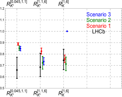
Figure 1: Comparison of the experimental measurements of $R_{K}$ and $R_{K^{*}}$ with the predictions of the three scenarios.

The first thing one sees is that none of the three scenarios predict a value for $R_{K^{*}}$ in the low-$q^{2}$ bin that is in agreement (within $1\sigma$) with the experimental measurement [Eq. (1)]. In the SM, in this $q^{2}$ region, the decay $b\to s\ell^{+}\ell^{-}$ is dominated by the photon contribution, parametrized by the WC $C_{7}$ RK*theory . Since the photon coupling is lepton flavor universal, it is only threshold effects, with $m_{\mu}\neq m_{e}$, that lead to $R_{K^{*}}^{\rm SM}\simeq 0.93$ flavio . It is difficult to find NP that can compete with the photon contribution and significantly change $R_{K^{*}}$ from its SM prediction. On the other hand, the discrepancy between the measurement and the predictions is only at the level of approximately $1.5\sigma$, which is not worrisome.

The predictions for the remaining measurements agree with the experimental values, with one glaring exception. Scenario (III) predicts $R_{K}=1$, as in the SM. This is in disagreement with the measurement [Eq. (2)].

As was shown in Sec. III.2, when $R_{K^{*}}$ and $R_{K}$ are included in the fit [fit (B)], the overall result with scenario (III) is good (a pull of 5.6). This scenario can therefore be considered a possible explanation for the $B$-decay anomalies. (Indeed, this is the conclusion of Ref. Capdevila:2017bsm .) However, in our opinion, this is not sufficient. As we saw above, scenario (III) predicts a value for $R_{K}$ that is in striking disagreement with the measurement. Furthermore, $R_{K}$ is a clean observable, i.e., it has very little theoretical uncertainty, so theoretical error cannot be a reason for the disagreement. The only reason fit (B) gives a good fit is that the $R_{K}$ measurement is only one of many, so its effect is diminished. However, we feel that this is misleading: given its clear failure to explain the measured value of $R_{K}$, scenario (III) should be considered as strongly disfavored, compared to scenarios (I) and (II).

$R_{K^{*}}$ and $R_{K}$ have been measured in the region of $q^{2}\leq 6$ $\rm GeV^{2}$. It is likely that these observables will also be measured in the region $15\leq q^{2}\leq 22$ $\rm GeV^{2}$. Below we present the predictions of the three scenarios for $R_{K^{*}}$ and $R_{K}$ in this high-$q^{2}$ bin:

$$R_{K^{*}} ~{}=~{} 0.76\pm 0.03~{}({\rm I})~{}~{},~{}~{}~{}~{}0.71\pm 0.06~{}({\rm II})~{}~{},~{}~{}~{}~{}0.68\pm 0.04~{}({\rm III})~{},$$

$$R_{K} ~{}=~{} 0.76\pm 0.03~{}({\rm I})~{}~{},~{}~{}~{}~{}0.72\pm 0.05~{}({\rm II})~{}`,~{}~{}~{}~{}1.0~{}({\rm III})~{}.$$ (6)

IV Model-dependent analysis

The simplest NP models one can construct that explain the $B$ anomalies involve the tree-level exchange of a new particle. This particle can be either a leptoquark or a $Z^{\prime}$ boson. Below we examine the properties of such NP models required for them to account for the $b\to s\mu^{+}\mu^{-}$ decays.

IV.1 Leptoquarks

LQ models were studied in detail in Ref. bsmumuCPV . It was found that, of the ten LQ models that couple to SM particles through dimension $\leq 4$ operators, only three can explain the $b\to s\mu^{+}\mu^{-}$ data. They are: a scalar isotriplet with $Y=1/3$, a vector isosinglet with $Y=-2/3$, and a vector isotriplet with $Y=-2/3$. These are denoted $S_{3}$, $U_{1}$ and $U_{3}$, respectively Sakakietal . As far as the $b\to s\mu^{+}\mu^{-}$ processes are concerned, the models all have $C_{9}^{\mu\mu}({\rm NP})=-C_{10}^{\mu\mu}({\rm NP})$, and so are equivalent. That is, all LQ models fall within scenario (II) of Eq. (4).

The $S_{3}$, $U_{1}$ and $U_{3}$ LQ models all contribute differently to $b\to s\nu_{\mu}{\bar{\nu}}_{\mu}$ decays, so that, in principle, they can be distinguished. However, it was shown in Ref. bsmumuCPV that the present constraints from $B\to K^{(*)}\nu{\bar{\nu}}$ are far weaker than those from $b\to s\mu^{+}\mu^{-}$ processes, so that the current $b\to s\nu{\bar{\nu}}$ data cannot be used to distinguish the three LQ models. (This said, this conclusion can be evaded if the LQs couple to other leptons, see Ref. RKRDmodels for an example.)

The bottom line is that there is effectively only a single LQ model that can explain the $B$-decay anomalies, and it is of type scenario (II). In order to determine the value of the WC required to reproduce the $b\to s\mu^{+}\mu^{-}$ data, a fit to this data is required, including all other processes to which this type of NP contributes. In this case, the only additional process is $b\to s\nu_{\mu}{\bar{\nu}}_{\mu}$, which does not furnish any additional constraints. The allowed value of the WC is therefore the same as that found in the model-independent fit, in Table 1 or 2.

This $b\to s\mu^{+}\mu^{-}$ WC is generated by the tree-level exchange of a LQ. Thus,

$$C_{9}^{\mu\mu}({\rm NP})\propto\frac{g_{L}^{b\mu}g_{L}^{b\mu}}{M_{\rm LQ}^{2}}~{},$$ (7)

where $g_{L}^{b\mu}$ and $g_{L}^{s\mu}$ are the couplings of the LQ (taken to be real), and $M_{\rm LQ}$ its mass. Direct searches constrain $M_{\rm LQ}>640$ GeV LQmasslimits .

IV.2 $Z^{\prime}$ bosons

In the previous subsection, we saw that LQ models are all of type scenario (II). This implies that scenarios (I) and (III) can only occur within $Z^{\prime}$ models. Is this possible? The four-fermion $b\to s\mu^{+}\mu^{-}$ operators required within the four scenarios are as follows:

$${\rm(I)} ~{}~{}~{}[{\bar{s}}\gamma_{\mu}P_{L}b][{\bar{\mu}}\gamma^{\mu}\mu]~{},$$ (8)

$${\rm(II)} ~{}~{}~{}[{\bar{s}}\gamma_{\mu}P_{L}b][{\bar{\mu}}\gamma^{\mu}P_{L}\mu]~{},$$

$${\rm(III)} ~{}~{}~{}[{\bar{s}}\gamma_{\mu}\gamma_{5}b][{\bar{\mu}}\gamma^{\mu}\mu]~{}.$$

Scenarios (I) and (II) are clearly allowed. They require the $Z^{\prime}$ to couple vectorially to ${\bar{s}}_{L}b_{L}$ and ${\bar{\mu}}\mu$ or ${\bar{\mu}}_{L}\mu_{L}$. It is quite natural for gauge bosons to couple vectorially, so it is easy to construct models which lead to scenario (I) or (II). On the other hand, scenario (III) requires that the $Z^{\prime}$ couple axial-vectorially to ${\bar{s}}b$. This is much less natural. It is possible to arrange this, but it requires a rather contrived model (e.g., see Ref. Capdevila:2017bsm ). Furthermore, we have already seen that scenario (III) is strongly disfavored by the $R_{K}$ measurement. In light of all this, we therefore exclude scenario (III) as a realistic explanation of the $B$-decay anomalies.

The conclusion is that, when model-independent and model-dependent considerations are combined, only scenarios (I) and (II) are possible as explanations of the $B$-decay anomalies. Furthermore, while scenario (II) can be realized with a LQ or $Z^{\prime}$ model, scenario (I) can only be due to $Z^{\prime}$ exchange.

Since the $Z^{\prime}$ couples to two left-handed quarks, it must transform as a singlet or triplet of $SU(2)_{L}$. The triplet option has been considered in Refs. CCO ; Crivellin:2015lwa ; Isidori ; dark ; Chiang ; Virto . (In this case, there is also a $W^{\prime}$ that can contribute to ${\bar{B}}\to D^{(*)+}\tau^{-}{\bar{\nu}}_{\tau}$ RKRD , another decay whose measurement exhibits a discrepancy with the SM RD_BaBar ; RD_Belle ; RD_LHCb .) Alternatively, if the $Z^{\prime}$ is a singlet of $SU(2)_{L}$, it must be the gauge boson associated with an extra $U(1)^{\prime}$. Numerous models of this type have been proposed, see Refs. GGH ; BG ; BFG ; Perimeter ; CDH ; SSV ; CHMNPR ; CMJS ; BDW ; FNZ ; Carmona:2015ena ; AQSS ; CFL ; Hou ; CHV ; CFV ; CFGI ; IGG ; BdecaysDM ; ZMeV ; Megias:2017ove ; Ahmed:2017vsr .

The vast majority of $Z^{\prime}$ models that have been proposed assume a heavy $Z^{\prime}$, $M_{Z^{\prime}}=$ O(TeV). This option is examined in Sec. IV.2.1. However, we also note that the $Z^{\prime}$ can be light. The cases of $M_{Z^{\prime}}=10$ GeV or 200 MeV are considered in Sec. IV.2.2.

IV.2.1 Heavy $Z^{\prime}$

In order to determine the properties of $Z^{\prime}$ models that explain the $b\to s\mu^{+}\mu^{-}$ data, one cannot simply perform fits (A) or (B) – important constraints from other observables must be taken into account. Since the $Z^{\prime}$ model is of the type scenario (I) or (II), we can write

$$\Delta{\cal L}_{Z^{\prime}} = J^{\mu}Z^{\prime}_{\mu}~{},$$

$${\rm where}\qquad J^{\mu} = g_{L}^{\mu\mu}\,\bar{L}\gamma^{\mu}P_{L}L+g_{R}^{\mu\mu}\,\bar{\mu}\gamma^{\mu}P_{R}\mu+g_{L}^{bs}\,{\bar{\psi}}_{q2}\gamma^{\mu}P_{L}\psi_{q3}+h.c.$$ (9)

Here $\psi_{qi}$ is the quark doublet of the $i^{th}$ generation, and $L=(\nu_{\mu},\mu)^{T}$. We have

scenario (I) $$~{}~{}:~{}~{} g_{R}^{\mu\mu}=g_{L}^{\mu\mu}~{},$$

scenario (II) $$~{}~{}:~{}~{} g_{R}^{\mu\mu}=0~{}.$$ (10)

When the heavy $Z^{\prime}$ is integrated out, we obtain the following effective Lagrangian containing 4-fermion operators:

$${\cal L}_{Z^{\prime}}^{eff}=-\frac{1}{2M_{Z^{\prime}}^{2}}J_{\mu}J^{\mu} \supset -\frac{g_{L}^{bs}}{M_{Z^{\prime}}^{2}}(\bar{s}\gamma^{\mu}P_{L}b)(\bar{\mu}\gamma^{\mu}(g_{L}^{\mu\mu}P_{L}+g_{R}^{\mu\mu}P_{R})\mu)-\frac{(g_{L}^{bs})^{2}}{2M_{Z^{\prime}}^{2}}(\bar{s}\gamma^{\mu}P_{L}b)(\bar{s}\gamma^{\mu}P_{L}b)$$ (11)

$$\hskip 14.22636pt-~{}\frac{g_{L}^{\mu\mu}}{M_{Z^{\prime}}^{2}}(\bar{\mu}\gamma^{\mu}(g_{L}^{\mu\mu}P_{L}+g_{R}^{\mu\mu}P_{R})\mu)({\bar{\nu}}_{\mu}\gamma^{\mu}P_{L}\nu_{\mu})~{}.$$

The first 4-fermion operator is relevant for $b\to s\mu^{+}\mu^{-}$ transitions, the second operator contributes to $B^{0}_{s}$-${\bar{B}}^{0}_{s}$ mixing, and the third operator contributes to neutrino trident production.

$\bullet$ $B^{0}_{s}$-${\bar{B}}^{0}_{s}$ mixing:

The formalism leading to the constraint on $g_{L}^{bs}$ from $B^{0}_{s}$-${\bar{B}}^{0}_{s}$ mixing is given in Ref. bsmumuCPV . We do not repeat it here. The one thing to keep in mind is that Ref. bsmumuCPV considered a complex $g_{L}^{bs}$, while here it is taken to be real.

$\bullet$ Neutrino trident production:

The production of $\mu^{+}\mu^{-}$ pairs in neutrino-nucleus scattering, $\nu_{\mu}N\to\nu_{\mu}N\mu^{+}\mu^{-}$ (neutrino trident production), is a powerful probe of new-physics models trident . The heavy $Z^{\prime}$ contribution to this process is also given in Ref. bsmumuCPV . However, there only scenario (II) ($g_{R}^{\mu\mu}=0$) is considered. Allowing for a nonzero $g_{R}^{\mu\mu}$, one obtains the following: the theoretical prediction for the cross section is

$$\left.{\sigma_{\text{SM+NP}}\over\sigma_{\text{SM}}}\right|_{\nu N\to\nu N\mu^{+}\mu^{-}}=\frac{1}{1+(1+4s_{W}^{2})^{2}}\left[\left(1+\frac{v^{2}g_{L}^{\mu\mu}(g_{L}^{\mu\mu}-g_{R}^{\mu\mu})}{M_{{Z}^{{}^{\prime}}}^{2}}\right)^{2}+\left(1+4s_{W}^{2}+\frac{v^{2}g_{L}^{\mu\mu}(g_{L}^{\mu\mu}+g_{R}^{\mu\mu})}{M_{{Z}^{{}^{\prime}}}^{2}}\right)^{2}\right]~{}.$$ (12)

This is to be compared with the experimental measurement CCFR :

$$\left.{\sigma_{\text{exp.}}\over\sigma_{\text{SM}}}\right|_{\nu N\to\nu N\mu^{+}\mu^{-}}=0.82\pm 0.28~{}.$$ (13)

Using Eq. (10), this comparison provides an upper limit on $(g_{L}^{\mu\mu})^{2}/M_{Z^{\prime}}^{2}$. For $M_{Z^{\prime}}=1$ TeV and $v=246$ GeV, we obtain the following $1\sigma$ upper bound on the coupling:

$${\rm(I)}:~{}~{}~{}~{}~{}|g_{L}^{\mu\mu}|\leq 0.99~{},$$

$${\rm(II)}:~{}~{}~{}~{}~{}|g_{L}^{\mu\mu}|\leq 1.38~{}.$$ (14)

$\bullet$ $b\to s\mu^{+}\mu^{-}$:

The couplings $g_{L}^{bs}$ and $g_{L,R}^{\mu\mu}$ are all involved in $b\to s\mu^{+}\mu^{-}$:

$$C_{9}^{\mu\mu}({\rm NP}) = -\left[\frac{\pi}{\sqrt{2}G_{F}\alpha V_{tb}V_{ts}^{*}}\right]\,\frac{g_{L}^{bs}(g_{L}^{\mu\mu}+g_{R}^{\mu\mu})}{M_{Z^{\prime}}^{2}}~{},$$

$$C_{10}^{\mu\mu}({\rm NP}) = \left[\frac{\pi}{\sqrt{2}G_{F}\alpha V_{tb}V_{ts}^{*}}\right]\,\frac{g_{L}^{bs}(g_{L}^{\mu\mu}-g_{R}^{\mu\mu})}{M_{Z^{\prime}}^{2}}~{}.$$ (15)

We see that any analysis of $Z^{\prime}$ models must include the constraints from $B^{0}_{s}$-${\bar{B}}^{0}_{s}$ mixing and neutrino trident production. And this applies to scenario (I), which, though supposedly model-independent, is related to $Z^{\prime}$ models.

The results of fits (A) and (B) are given in Tables 3 and 4, respectively. These illustrate quite clearly the connection between the model-independent and model-dependent approaches. From the model-independent point of view, in order to explain the experimental data, the NP WC must take a certain value (given in Tables 1 and 2). However, from the model-dependent point of view, this WC is proportional to the product $g_{L}^{bs}g_{L}^{\mu\mu}$ [Eq. (15), using Eq. (10)], and these individual couplings have additional constraints from other processes. $g_{L}^{\mu\mu}$ is constrained by neutrino trident production [Eq. (14)]. Now, if $g_{L}^{\mu\mu}$ is small, $g_{L}^{bs}$ must be large in order to reproduce the required WC. However, a large $g_{L}^{bs}$ is in conflict with the constraint from $B^{0}_{s}$-${\bar{B}}^{0}_{s}$ mixing, resulting in a poorer fit (i.e., a smaller pull). On the other hand, if $g_{L}^{\mu\mu}$ is large (but still consistent with Eq. (14)), $g_{L}^{bs}$ can be small, so that the $B^{0}_{s}$-${\bar{B}}^{0}_{s}$ mixing constraint is less important. In this case, a good fit (i.e., a large pull) is possible. Indeed, for large enough $g_{L}^{\mu\mu}$, one simply reproduces the model-independent result. For both fits (A) and (B), we find that this is the case for $g_{L}^{\mu\mu}\geq 0.4$. The conclusion is that, if the NP is a $Z^{\prime}$, the coupling $g_{L}^{\mu\mu}$ has to be reasonably big. Its effect may be observable in a future experiment on neutrino trident production.

	$M_{Z^{\prime}}=1$ TeV
$g_{L}^{\mu\mu}$	$Z^{\prime}$ (I): $g_{L}^{bs}$ $\times 10^{3}$	pull
0.01	$-2.6\pm 1.9$	1.0
0.05	$-4.2\pm 1.1$	2.8
0.1	$-4.6\pm 0.9$	4.0
0.2	$-3.8\pm 0.7$	4.8
0.4	$-2.2\pm 0.4$	5.0
0.5	$-1.8\pm 0.3$	5.0

	$M_{Z^{\prime}}=1$ TeV
$g_{L}^{\mu\mu}$	$Z^{\prime}$ (II): $g_{L}^{bs}$ $\times 10^{3}$	pull
0.01	$-2.4\pm 1.9$	1.0
0.05	$-4.0\pm 1.1$	2.8
0.1	$-3.6\pm 0.8$	3.6
0.2	$-3.8\pm 0.8$	4.3
0.4	$-2.3\pm 0.5$	4.6
0.5	$-1.9\pm 0.4$	4.6

Table 3: $Z^{\prime}$ model (scenario (I) : left, scenario (II) : right): best-fit value of $g_{L}^{bs}$, and the pull=$\sqrt{\chi^{2}_{SM}-\chi^{2}_{SM+NP}}$ for fit (A) (only CP-conserving $b\to s\mu^{+}\mu^{-}$ observables), for various values of $g_{L}^{\mu\mu}$.

	$M_{Z^{\prime}}=1$ TeV
$g_{L}^{\mu\mu}$	$Z^{\prime}$ (I): $g_{L}^{bs}$ $\times 10^{3}$	pull
0.01	$-3.0\pm 1.6$	1.4
0.05	$-4.8\pm 1.0$	2.8
0.1	$-5.2\pm 0.8$	4.5
0.2	$-4.2\pm 0.6$	5.7
0.4	$-2.4\pm 0.4$	5.9
0.5	$-1.9\pm 0.3$	5.9

	$M_{Z^{\prime}}=1$ TeV
$g_{L}^{\mu\mu}$	$Z^{\prime}$ (II): $g_{L}^{bs}$ $\times 10^{3}$	pull
0.01	$-3.0\pm 1.6$	1.4
0.05	$-4.8\pm 1.0$	2.8
0.1	$-5.2\pm 0.8$	4.5
0.2	$-4.4\pm 0.7$	5.6
0.4	$-2.5\pm 0.4$	5.9
0.5	$-2.1\pm 0.4$	5.9

Table 4: $Z^{\prime}$ model (scenario (I) : left, scenario (II) : right): best-fit value of $g_{L}^{bs}$, and the pull=$\sqrt{\chi^{2}_{SM}-\chi^{2}_{SM+NP}}$ for fit (B) (CP-conserving $b\to s\mu^{+}\mu^{-}$ observables $+$ $R_{K^{*}}$ and $R_{K}$), for various values of $g_{L}^{\mu\mu}$.

IV.2.2 Light $Z^{\prime}$

An interesting possibility to consider is a light $Z^{\prime}$. If the $Z^{\prime}$ mass is between $m_{B}$ and $2m_{\mu}$, then, if it is narrow, one can observe this state as a resonance in the dimuon invariant mass. Since no such state has been observed, we consider the mass ranges $m_{Z^{\prime}}>m_{B}$ and $m_{Z^{\prime}}<2m_{\mu}$. A $Z^{\prime}$ in the first mass range may have implications for dark matter phenomenology BdecaysDM , while a $Z^{\prime}$ in the second mass range could explain the muon $g-2$ measurement and have implications for nonstandard neutrino interactions ZMeV . For the first mass range we consider $M_{Z^{\prime}}=10$ GeV and refer to this as the GeV $Z^{\prime}$ model, while in the second range we consider $M_{Z^{\prime}}=200$ MeV and call it the MeV $Z^{\prime}$ model

For the MeV $Z^{\prime}$ model, we assume there is a flavor-changing ${\bar{s}}bZ^{\prime}$ vertex whose form is taken to be

$$F(q^{2})\,\bar{s}\gamma^{\mu}P_{L}b\,Z^{\prime}_{\mu}~{}.$$ (16)

The form factor $F(q^{2})$ is expanded for the momentum transfer $q^{2}\ll m_{B}^{2}$ as

$$F(q^{2}) = a^{bs}_{L}+g^{bs}_{L}\frac{q^{2}}{m_{B}^{2}}+\ldots\,,\$$ (17)

where $m_{B}$ is the $B$-meson mass. For the GeV $Z^{\prime}$ model there is no form factor, and the ${\bar{s}}bZ^{\prime}$ vertex is taken to be fixed at $a^{bs}_{L}$ for all $q^{2}$.

In the MeV $Z^{\prime}$ model, assuming the $Z^{\prime}$ couples to neutrinos, the leading-order term $a^{bs}_{L}$ is constrained by $B\to K\nu\bar{\nu}$ to be smaller than $10^{-9}$. To explain the $b\to s\mu^{+}\mu^{-}$ anomalies, we then require the $Z^{\prime}$ to have a large coupling to muons, which is inconsistent with data ZMeV . We therefore neglect $a^{bs}_{L}$ and keep only $g^{bs}_{L}$. (If the $Z^{\prime}$ does not couple to neutrinos then this constraint does not apply.) In the GeV $Z^{\prime}$ model $a^{bs}_{L}$ is present, so here we neglect $g^{bs}_{L}$.

The matrix elements for the various processes are then

$$M_{b\to s\mu^{+}\mu^{-}} = -\frac{F(q^{2})}{q^{2}-M_{Z^{\prime}}^{2}}(\bar{s}\gamma^{\mu}P_{L}b)(\bar{\mu}\gamma^{\mu}(g_{L}^{\mu\mu}P_{L}+g_{R}^{\mu\mu}P_{R})\mu)~{},$$

$$M_{{B_{s}}mix} = -\frac{F(q^{2})^{2}}{2q^{2}-2M_{Z^{\prime}}^{2}}(\bar{s}\gamma^{\mu}P_{L}b)(\bar{s}\gamma^{\mu}P_{L}b)\left[1-\frac{5}{8}\frac{m_{b}^{2}}{m_{Z^{\prime}}^{2}}\right]~{},$$

$$M_{trident} = -~{}\frac{g_{L}^{\mu\mu}}{q^{2}-M_{Z^{\prime}}^{2}}(\bar{\mu}\gamma^{\mu}(g_{L}^{\mu\mu}P_{L}+g_{R}^{\mu\mu}P_{R})\mu)({\bar{\nu}}_{\mu}\gamma^{\mu}P_{L}\nu_{\mu})~{},$$ (18)

where we have used Ref. tandean for $B^{0}_{s}$-${\bar{B}}^{0}_{s}$ mixing. In $M_{b\to s\mu^{+}\mu^{-}}$ there is an additional contribution from the longitudinal $Z^{\prime}$ for the axial leptonic current that is $\sim m_{\mu}m_{b}/m_{Z^{\prime}}^{2}$. For the GeV $Z^{\prime}$ model this term can be neglected. However, for the MeV $Z^{\prime}$ model this term is sizeable, and so for this case we only consider scenario I with a vectorial leptonic current. As usual, we assume the $Z^{\prime}$ does not couple to electrons, so that ${\cal B}(B^{+}\to K^{+}e^{+}e^{-})$ is described by the SM, while ${\cal B}(B^{+}\to K^{+}\mu^{+}\mu^{-})$ is modified by NP.

$\bullet$ $B^{0}_{s}$-${\bar{B}}^{0}_{s}$ mixing:

The measurement of $B^{0}_{s}$-${\bar{B}}^{0}_{s}$ mixing gives a constraint on the product of couplings and the form factor. For the MeV $Z^{\prime}$ model, as the form factor at $q^{2}\sim m_{B}^{2}$ is not known, we fit $g_{L}^{bs}$ only from the $b\to s\mu^{+}\mu^{-}$ data, while for the GeV $Z^{\prime}$ model, where the form factor is unity, the mixing is used to obtain a constraint on $a_{L}^{bs}$.

$\bullet$ Neutrino trident production:

The coupling $g^{\mu\mu}$ is constrained by neutrino trident production. For the MeV $Z^{\prime}$ model, Eq. 12 is no longer valid – instead we use the constraints from Ref. trident . In this reference only scenario (I) ($g_{R}^{\mu\mu}=g_{L}^{\mu\mu}$) is considered. There are other constraints that the MeV $Z^{\prime}$ model must satisfy; these are discussed in Ref. Farzan . All these constraints are consistent with the constraint obtained from neutrino trident production.

$\bullet$ $b\to s\mu^{+}\mu^{-}$:

For $b\to s\mu^{+}\mu^{-}$ we have

$$C_{9}^{\mu\mu}({\rm NP}) = \left[\frac{\pi}{\sqrt{2}G_{F}\alpha V_{tb}V_{ts}^{*}}\right]\,\frac{\left(a_{L}^{bs}+g_{L}^{bs}(q^{2}/m_{B_{s}}^{2})\right)(g_{L}^{\mu\mu}+g_{R}^{\mu\mu})}{q^{2}-M_{Z^{\prime}}^{2}}~{},$$

$$C_{10}^{\mu\mu}({\rm NP}) = -\left[\frac{\pi}{\sqrt{2}G_{F}\alpha V_{tb}V_{ts}^{*}}\right]\,\frac{\left(a_{L}^{bs}+g_{L}^{bs}(q^{2}/m_{B_{s}}^{2})\right)(g_{L}^{\mu\mu}-g_{R}^{\mu\mu})}{q^{2}-M_{Z^{\prime}}^{2}}~{}.$$ (19)

Interestingly, here the WCs are $q^{2}$-dependent.

Using these WCs, we perform a fit to the data. We scan the parameter space of $g_{bs}$ and $g_{\mu\mu}$ for values that are consistent with all experimental measurements. For the MeV $Z^{\prime}$ model, the form factor is not known in the high-$q^{2}$ region, and so one can fit only to the low-$q^{2}$ bins. However, we have checked that the fit does not change much if we use the above form factor for all $q^{2}$ bins. For both the MeV and GeV $Z^{\prime}$ we find that, in fact, it is possible to explain the $B$-decay anomalies with pulls that are almost as good as in the case of a heavy $Z^{\prime}$.

For the MeV $Z^{\prime}$ model, the best fit has a pull of 4.4, and is found for the product of couplings $g_{L}^{bs}g_{L}^{\mu\mu}\sim 21\times 10^{-9}$. Taking $g_{L}^{\mu\mu}\sim 10^{-3}$ from the neutrino trident constraint, one obtains $g_{L}^{bs}\sim 2.1\times 10^{-5}$, which is consistent with constraints from $B\to K\nu\bar{\nu}$ ZMeV . The results for the GeV $Z^{\prime}$ model are shown in Table 5 for fit (A). The best fit has a pull of 4.2 (scenario (I)) or 4.5 (scenario (II)).

	$M_{Z^{\prime}}=10$ GeV
$g_{L}^{\mu\mu}$ $\times 10^{2}$	$Z^{\prime}$ (I): $g_{L}^{bs}$ $\times 10^{6}$	pull
0.05	$-36.3\pm 10.2$	2.6
0.1	$-37.6\pm 8.5$	3.6
0.3	$-20.2\pm 4.6$	4.1
0.6	$-10.3\pm 2.3$	4.2
0.9	$-6.9\pm 1.6$	4.2
1.2	$-5.2\pm 1.2$	4.2

	$M_{Z^{\prime}}=10$ GeV
$g_{L}^{\mu\mu}$ $\times 10^{2}$	$Z^{\prime}$ (II): $g_{L}^{bs}$ $\times 10^{6}$	pull
0.05	$-35.4\pm 11.0$	2.8
0.1	$-38.7\pm 9.0$	3.4
0.3	$-27.0\pm 6.2$	4.3
0.6	$-14.4\pm 3.6$	4.5
0.9	$-9.6\pm 2.3$	4.5
1.2	$-7.2\pm 1.8$	4.5

Table 5: GeV $Z^{\prime}$ model (scenario (I) : left, scenario (II) : right): best-fit value of $g_{L}^{bs}$, and the pull=$\sqrt{\chi^{2}_{SM}-\chi^{2}_{SM+NP}}$ in fit (A), for various values of $g_{L}^{\mu\mu}$.

As noted in the discussion about Fig. 1, the value of $R_{K^{*}}$ in the low-$q^{2}$ bin ($0.045\leq q^{2}\leq 1.1~{}{\rm GeV}^{2}$) is dominated by the SM photon contribution. Heavy NP cannot significantly affect this, and so cannot much improve the discrepancy between the measurement and the SM prediction of $R_{K^{*}}$ in this bin. On the other hand, since the WCs are $q^{2}$-dependent in light-$Z^{\prime}$ models, in principal they could have a large effect on this value of $R_{K^{*}}$. Unfortunately, for $M_{Z^{\prime}}=10$ GeV and 200 MeV, we find that the prediction for $R_{K^{*}}$ in the low-$q^{2}$ bin is little changed from that of the SM. However, this might not hold in a different version of a light $Z^{\prime}$ model (for example, see Ref. Ghosh:2017ber ).

V Conclusions

Following the announcement of the measurement of $R_{K^{*}}$ RK*expt , a flurry of papers appeared Capdevila:2017bsm ; Altmannshofer:2017yso ; DAmico:2017mtc ; Hiller:2017bzc ; Geng:2017svp ; Ciuchini:2017mik ; Celis:2017doq ; DiChiara:2017cjq ; Sala:2017ihs ; Ghosh:2017ber discussing how to explain the result and what it implies for new physics. Most papers adopted a model-independent approach, while a few focused on particular models. The main purpose of the present paper is to show that additional information about the NP is available if one combines the model-independent and model-dependent analyses.

To be specific, the general preference was for NP in $b\to s\mu^{+}\mu^{-}$ transitions (although some papers considered the possibility of NP in both $b\to s\mu^{+}\mu^{-}$ and $b\to se^{+}e^{-}$). Several model-independent studies pointed out that the $b\to s\mu^{+}\mu^{-}$ anomalies can be explained if (I) $C_{9}^{\mu\mu}({\rm NP})<0$ or (II) $C_{9}^{\mu\mu}({\rm NP})=-C_{10}^{\mu\mu}({\rm NP})<0$. We agree with this observation. Now, the simplest NP models involve the tree-level exchange of a leptoquark (LQ) or a $Z^{\prime}$ boson. A number of different LQ models have previously been proposed, but we point out that, as far as the $b\to s\mu^{+}\mu^{-}$ processes are concerned, all viable models have $C_{9}^{\mu\mu}({\rm NP})=-C_{10}^{\mu\mu}({\rm NP})$, and so are equivalent. That is, there is effectively a single LQ model, and it falls within scenario (II).

The key point is that, although scenario (II) can arise in LQ or $Z^{\prime}$ models, scenario (I) is only possible with a $Z^{\prime}$. Thus, analyses that favor NP in $C_{9}^{\mu\mu}$ only are essentially favoring models in which $b\to s\mu^{+}\mu^{-}$ arises due to $Z^{\prime}$ exchange. We have performed a model-dependent analysis of $Z^{\prime}$ models, taking into account the additional constraints from $B^{0}_{s}$-${\bar{B}}^{0}_{s}$ mixing and neutrino trident production. If the $Z^{\prime}$ is heavy, $M_{Z^{\prime}}=$ O(TeV), the ${\bar{\mu}}\mu Z^{\prime}$ coupling is reasonably large, and could have an observable effect in a future experiment on neutrino trident production. We also find that a good fit to the data is found if the $Z^{\prime}$ is light, $M_{Z^{\prime}}=10$ GeV or 200 MeV.

Finally, a third scenario, (III) $C_{9}^{\mu\mu}({\rm NP})=-C_{9}^{\prime\mu\mu}({\rm NP})$ has also been proposed as an explanation for the $b\to s\mu^{+}\mu^{-}$ data. We note that this scenario predicts $R_{K}=1$, in disagreement with the experiment. In addition, this scenario can only arise in rather contrived models. For these reasons, we exclude scenario (III) as an explanation of the $B$-decay anomalies.

Acknowledgements: This work was financially supported by by the U. S. Department of Energy under contract DE-SC0007983 (BB), by the National Science Foundation under Grant No. PHY-1414345 (AD), and by NSERC of Canada (DL). AD thanks Xerxes Tata for helpful conversations. JK wishes to thank Bibhuprasad Mahakud for discussions and technical help regarding the global fits.

Appendix

This Appendix contains Tables of all $b\to s\mu^{+}\mu^{-}$ experimental data used in the fits.

$B^{0}\to K^{*0}\mu^{+}\mu^{-}$ differential branching ratio
Bin (GeV2)	Measurement ($\times 10^{7}$)
LHCb 2016 Aaij:2016flj
$[1.1,2.5]$	$0.326_{\,-0.031}^{\,+0.032}\pm{0.010}\pm 0.022$
$[2.5,4.0]$	$0.334_{\,-0.033}^{\,+0.031}\pm{0.009}\pm 0.023$
$[4.0,6.0]$	$0.354_{\,-0.026}^{\,+0.027}\pm{0.009}\pm 0.024$
$[15.0,19.0]$	$0.436_{\,-0.019}^{\,+0.018}\pm{0.007}\pm 0.030$
CDF CDFupdate
$[0.0,2.0]$	$0.912\pm 1.73\pm 0.49$
$[2.0,4.3]$	$0.461\pm 1.19\pm 0.27$
CMS 2013 Chatrchyan:2013cda
$[1.0,2.0]$	$0.48^{+0.14}_{-0.12}\pm 0.04$
$[2.0,4.3]$	$0.38\pm 0.07\pm 0.03$
CMS 2015 Khachatryan:2015isa
$[1.0,2.0]$	$0.46\pm 0.07\pm 0.03$
$[2.0,4.3]$	$0.33\pm 0.05\pm 0.02$

Table 6: Experimental measurements of the differential branching ratio of $B^{0}\to K^{*0}\mu^{+}\mu^{-}$.

$B^{0}\to K^{*0}\mu^{+}\mu^{-}$ angular observables
ATLAS 2017 BK*mumuATLAS
$q^{2}\in[\,0.04\,,\,2.0\,]\,{\rm GeV}^{2}$	$q^{2}\in[\,2.0\,,\,4.0\,]\,{\rm GeV}^{2}$	$q^{2}\in[\,4.0\,,\,6.0\,]\,{\rm GeV}^{2}$
$\langle F_{L}\rangle=\phantom{-}0.44\,\pm 0.08\pm 0.07$	$\langle F_{L}\rangle=\phantom{-}0.64\pm 0.11\pm 0.05$	$\langle F_{L}\rangle=\phantom{-}0.42\pm 0.13\pm 0.12$
$\langle S_{3}\rangle=-\phantom{-}0.02\,\pm 0.09\pm 0.02$	$\langle S_{3}\rangle=-\phantom{-}0.15\pm 0.10\pm 0.07$	$\langle S_{3}\rangle=\phantom{-}0.00\pm 0.12\pm 0.07$
$\langle S_{4}\rangle=\phantom{-}0.19\,\pm 0.25\pm 0.10$	$\langle S_{4}\rangle=-\phantom{-}0.47\pm 0.19\pm 0.10$	$\langle S_{4}\rangle=\phantom{-}0.40\pm 0.21\pm 0.09$
$\langle S_{5}\rangle=\phantom{-}0.33\,\pm 0.13\pm 0.06$	$\langle S_{5}\rangle=-\phantom{-}0.16\pm 0.15\pm 0.05$	$\langle S_{5}\rangle=\phantom{-}0.13\pm 0.18\pm 0.07$
$\langle S_{7}\rangle=-\phantom{-}0.09\,\pm 0.10\pm 0.02$	$\langle S_{7}\rangle=\phantom{-}0.15\pm 0.14\pm 0.09$	$\langle S_{7}\rangle=\phantom{-}0.03\pm 0.13\pm 0.07$
$\langle S_{8}\rangle=-\phantom{-}0.11\,\pm 0.19\pm 0.07$	$\langle S_{8}\rangle=\phantom{-}0.41\pm 0.16\pm 0.15$	$\langle S_{8}\rangle=-\phantom{-}0.09\pm 0.16\pm 0.04$
CMS 2017 BK*mumuCMS
$q^{2}\in[\,1.0\,,\,2.0\,]\,{\rm GeV}^{2}$	$q^{2}\in[\,2.0\,,\,4.3\,]\,{\rm GeV}^{2}$	$q^{2}\in[\,4.3\,,\,6.0\,]\,{\rm GeV}^{2}$
$\langle P_{1}\rangle=\phantom{-}0.12\,{}^{+0.46}_{-0.47}\pm 0.06$	$\langle P_{1}\rangle=-\phantom{-}0.69\,{}^{+0.58}_{-0.27}\pm 0.09$	$\langle P_{1}\rangle=\phantom{-}0.53\,{}^{+0.24}_{-0.33}\pm 0.18$
$\langle P^{\prime}_{5}\rangle=\phantom{-}0.10\,{}^{+0.32}_{-0.31}\pm 0.12$	$\langle P^{\prime}_{5}\rangle=-\phantom{-}0.57\,{}^{+0.34}_{-0.31}\pm 0.15$	$\langle P^{\prime}_{5}\rangle=-\phantom{-}0.96\,{}^{+0.22}_{-0.21}\pm 0.16$
CMS 2015 Khachatryan:2015isa
$q^{2}\in[\,1.0\,,\,2.0\,]\,{\rm GeV}^{2}$	$q^{2}\in[\,2.0\,,\,4.3\,]\,{\rm GeV}^{2}$	$q^{2}\in[\,4.3\,,\,6.0\,]\,{\rm GeV}^{2}$
$\langle F_{L}\rangle=\phantom{-}0.64\,{}^{+0.10}_{-0.09}\pm 0.07$	$\langle F_{L}\rangle=\phantom{-}0.80\pm 0.08\pm 0.06$	$\langle F_{L}\rangle=\phantom{-}0.62\,{}^{+0.10}_{-0.09}\pm 0.07$
$\langle A_{FB}\rangle=-\phantom{-}0.27\,{}^{+0.17}_{-0.40}\pm 0.07$	$\langle A_{FB}\rangle=-\phantom{-}0.12\,{}^{+0.15}_{-0.17}\pm 0.05$	$\langle A_{FB}\rangle=-\phantom{-}0.01\pm 0.15\pm 0.03$
LHCb 2015 BK*mumuLHCb2
$q^{2}\in[\,1.1\,,\,2.5\,]\,{\rm GeV}^{2}$	$q^{2}\in[\,2.5\,,\,4.0\,]\,{\rm GeV}^{2}$	$q^{2}\in[\,4.0\,,\,6.0\,]\,{\rm GeV}^{2}$
$\langle F_{L}\rangle=\phantom{-}0.660\,{}^{+0.083}_{-0.077}\pm 0.022$	$\langle F_{L}\rangle=\phantom{-}0.876\,{}^{+0.109}_{-0.097}\pm 0.017$	$\langle F_{L}\rangle=\phantom{-}0.611\,{}^{+0.052}_{-0.053}\pm 0.017$
$\langle A_{FB}\rangle=-0.191\,{}^{+0.068}_{-0.080}\pm 0.012$	$\langle A_{FB}\rangle=-0.118\,{}^{+0.082}_{-0.090}\pm 0.007$	$\langle A_{FB}\rangle=\phantom{-}0.025\,{}^{+0.051}_{-0.052}\pm 0.004$
$\langle S_{3}\rangle=-0.077\,{}^{+0.087}_{-0.105}\pm 0.005$	$\langle S_{3}\rangle=\phantom{-}0.035\,{}^{+0.098}_{-0.089}\pm 0.007$	$\langle S_{3}\rangle=\phantom{-}0.035\,{}^{+0.069}_{-0.068}\pm 0.007$
$\langle S_{4}\rangle=-0.077\,{}^{+0.111}_{-0.113}\pm 0.005$	$\langle S_{4}\rangle=-0.234\,{}^{+0.127}_{-0.144}\pm 0.006$	$\langle S_{4}\rangle=-0.219\,{}^{+0.086}_{-0.084}\pm 0.008$
$\langle S_{5}\rangle=\phantom{-}0.137\,{}^{+0.099}_{-0.094}\pm 0.009$	$\langle S_{5}\rangle=-0.022\,{}^{+0.110}_{-0.103}\pm 0.008$	$\langle S_{5}\rangle=-0.146\,{}^{+0.077}_{-0.078}\pm 0.011$
$\langle S_{7}\rangle=-0.219\,{}^{+0.094}_{-0.104}\pm 0.004$	$\langle S_{7}\rangle=\phantom{-}0.068\,{}^{+0.120}_{-0.112}\pm 0.005$	$\langle S_{7}\rangle=-0.016\,{}^{+0.081}_{-0.080}\pm 0.004$
$\langle S_{8}\rangle=-0.098\,{}^{+0.108}_{-0.123}\pm 0.005$	$\langle S_{8}\rangle=\phantom{-}0.030\,{}^{+0.129}_{-0.131}\pm 0.006$	$\langle S_{8}\rangle=\phantom{-}0.167\,{}^{+0.094}_{-0.091}\pm 0.004$
$\langle S_{9}\rangle=-0.119\,{}^{+0.087}_{-0.104}\pm 0.005$	$\langle S_{9}\rangle=-0.092\,{}^{+0.105}_{-0.125}\pm 0.007$	$\langle S_{9}\rangle=-0.032\,{}^{+0.071}_{-0.071}\pm 0.004$
$q^{2}\in[\,15.0\,,\,19.0\,]\,{\rm GeV}^{2}$
$\langle F_{L}\rangle=\phantom{-}0.344\,{}^{+0.028}_{-0.030}\pm 0.008$
$\langle A_{FB}\rangle=-\phantom{-}0.355\,{}^{+0.027}_{-0.027}\pm 0.009$
$\langle S_{3}\rangle=-0.163\,{}^{+0.033}_{-0.033}\pm 0.009$
$\langle S_{4}\rangle=-0.284\,{}^{+0.038}_{-0.041}\pm 0.007$
$\langle S_{5}\rangle=-0.325\,{}^{+0.036}_{-0.037}\pm 0.009$
$\langle S_{7}\rangle=\phantom{-}0.048\,{}^{+0.043}_{-0.043}\pm 0.006$
$\langle S_{8}\rangle=\phantom{-}0.028\,{}^{+0.044}_{-0.045}\pm 0.003$
$\langle S_{9}\rangle=-0.053\,{}^{+0.039}_{-0.039}\pm 0.002$
CDF
$q^{2}\in[\,0.0\,,\,2.0\,]\,{\rm GeV}^{2}$	$q^{2}\in[\,2.0\,,\,4.3\,]\,{\rm GeV}^{2}$
$\langle F_{L}\rangle=\phantom{-}0.26\,{}^{+0.14}_{-0.13}\pm 0.04$	$\langle F_{L}\rangle=\phantom{-}0.72\,{}^{+0.15}_{-0.17}\pm 0.09$
$\langle A_{FB}\rangle=\phantom{-}0.07\,{}^{+0.29}_{-0.28}\pm 0.11$	$\langle A_{FB}\rangle=-\phantom{-}0.11\,{}^{+0.34}_{-0.45}\pm 0.16$

Table 7: Experimental measurements of the angular observables of $B^{0}\to K^{*0}\mu^{+}\mu^{-}$.

$B^{+}\to K^{*+}\mu^{+}\mu^{-}$ differential branching ratio
LHCb 2014 Aaij:2014pli
Bin (GeV2)	Measurement($\times 10^{9}$)
$[0.1-2.0]$	$59.2^{+14.4}_{-13.0}\pm 4.0$
$[2.0-4.0]$	$55.9^{+15.9}_{-14.4}\pm 3.8$
$[4.0-6.0]$	$24.9^{+11.0}_{-9.6}\pm 1.7$
$[15.0-19.0]$	$39.5^{+8.0}_{-7.3}\pm 2.8$
CDF CDFupdate
$[0.0-2.0]$	$75.0\pm+46.8\pm 8.8$
$[2.0-4.0]$	$49.4\pm 35.8\pm 6.3$

Table 8: Experimental measurements of the differential branching ratio of $B^{+}\to K^{*+}\mu^{+}\mu^{-}$.

$B^{+}\to K^{+}\mu^{+}\mu^{-}$ differential branching ratio
LHCb 2014 Aaij:2014pli
Bin (GeV2)	Measurement ($\times 10^{9}$)
$[1.1-2.0]$	$23.3\pm 1.5\pm 1.2$
$[2.0-3.0]$	$28.2\pm 1.6\pm 1.4$
$[3.0-4.0]$	$25.4\pm 1.5\pm 1.3$
$[4.0-5.0]$	$22.1\pm 1.4\pm 1.1$
$[5.0-6.0]$	$23.1\pm 1.4\pm 1.2$
$[15.0-22.0]$	$\phantom{0}12.1\pm 0.4\pm 0.6$
CDF CDFupdate
$[0.0-2.0]$	$18.0\pm 5.3\pm 1.2$
$[2.0-4.3]$	$31.6\pm 5.4\pm 1.8$

Table 9: Experimental measurements of the differential branching ratio of $B^{+}\to K^{+}\mu^{+}\mu^{-}$ .

$B^{0}\to K^{0}\mu^{+}\mu^{-}$ differential branching ratio
LHCb 2014 Aaij:2014pli
Bin (GeV2)	Measurement ($\times 10^{9}$)
$[0.1-2.0]$	$12.2^{+5.9}_{-5.2}\pm 0.6$
$[2.0-4.0]$	$18.7^{+5.5}_{-4.9}\pm 0.9$
$[4.0-6.0]$	$17.3^{+5.3}_{-4.8}\pm 0.9$
$[15.0-22.0]$	$\phantom{0}9.5^{+1.6}_{-1.5}\pm 0.5$
CDF CDFupdate
$[0.0-2.0]$	$24.5\pm 15.9\pm 2.1$
$[2.0-4.3]$	$25.5\pm 17.0\pm 3.5$

Table 10: Experimental measurements of the differential branching ratio of $B^{0}\to K^{0}\mu^{+}\mu^{-}$.

$B^{0}_{s}\to\phi\mu^{+}\mu^{-}$ differential branching ratio
Bin (GeV2)	Measurement ($\times 10^{8}$)
$[1.0-6.0]$	$2.58^{+0.33}_{-0.31}\pm{0.08}\pm{0.19}$
$[15.0-19.0]$	$4.04^{+0.39}_{-0.38}\pm{0.13}\pm{0.30}$

Table 11: Experimental measurements of the differential branching ratio of $B^{0}_{s}\to\phi\mu^{+}\mu^{-}$ BsphimumuLHCb2 . The experimental errors are, from left to right, statistical, systematic and due to the uncertainty on the branching ratio of the normalization mode $B^{0}_{s}\to J/\psi\phi$.

$B^{0}_{s}\to\phi\mu^{+}\mu^{-}$ angular observables
$q^{2}\in[\,0.1\,,\,2.0\,]\,{\rm GeV}^{2}$	$q^{2}\in[\,2.0\,,\,5.0\,]\,{\rm GeV}^{2}$
$\langle F_{L}\rangle=\phantom{-}0.20^{+0.08}_{-0.09}\pm 0.02$	$\langle F_{L}\rangle=\phantom{-}0.68^{+0.16}_{-0.13}\pm 0.03$
$\langle S_{3}\rangle=-0.05^{+0.13}_{-0.13}\pm 0.01$	$\langle S_{3}\rangle=-0.06^{+0.19}_{-0.23}\pm 0.01$
$\langle S_{4}\rangle=\phantom{-}0.27^{+0.28}_{-0.18}\pm 0.01$	$\langle S_{4}\rangle=-0.47^{+0.30}_{-0.44}\pm 0.01$
$\langle S_{7}\rangle=\phantom{-}0.04^{+0.12}_{-0.12}\pm 0.00$	$\langle S_{7}\rangle=-0.03^{+0.18}_{-0.23}\pm 0.01$
$q^{2}\in[\,15.0\,,\,19.0\,]\,{\rm GeV}^{2}$
$\langle F_{L}\rangle=\phantom{-}0.29^{+0.07}_{-0.06}\pm 0.02$
$\langle S_{3}\rangle=-0.09^{+0.11}_{-0.12}\pm 0.01$
$\langle S_{4}\rangle=-0.14^{+0.11}_{-0.11}\pm 0.01$
$\langle S_{7}\rangle=\phantom{-}0.13^{+0.11}_{-0.11}\pm 0.01$

Table 12: Experimental measurements of the angular observables of $B^{0}_{s}\to\phi\mu^{+}\mu^{-}$ BsphimumuLHCb2 . The experimental errors are, from left to right, statistical and systematic.

$B\to X_{s}\mu^{+}\mu^{-}$ differential branching ratio
Bin	Measurement ($\times 10^{6}$)
$q^{2}\in[1,6]~{}{\rm GeV}^{2}$	$0.66\pm{0.88}$
$q^{2}>14.2~{}{\rm GeV}^{2}$	$0.60\pm{0.31}$

Table 13: Experimental measurements of the differential branching ratio of $B\to X_{s}\mu^{+}\mu^{-}$ Lees:2013nxa .

References

- (1) S. Bifani (on behalf of the LHCb Collaboration), “Search for New Physics with decays at LHCb,” talk given at CERN, April 18, 2017.
- (2) See, for example, G. Hiller and F. Kruger, “More model-independent analysis of processes,” Phys. Rev. D 69, 074020 (2004) doi:10.1103/PhysRevD.69.074020 [hep-ph/0310219].
- (3) David Straub, flavio v0.11, 2016. http://dx.doi.org/10.5281/zenodo.59840
- (4) R. Aaij et al. [LHCb Collaboration], “Test of lepton universality using decays,” Phys. Rev. Lett. 113, 151601 (2014) [arXiv:1406.6482 [hep-ex]].
- (5) M. Bordone, G. Isidori and A. Pattori, “On the Standard Model predictions for and ,” Eur. Phys. J. C 76, no. 8, 440 (2016) doi:10.1140/epjc/s10052-016-4274-7 [arXiv:1605.07633 [hep-ph]].
- (6) See, for example, V. G. Chobanova, T. Hurth, F. Mahmoudi, D. Martinez Santos and S. Neshatpour, “Large hadronic power corrections or new physics in the rare decay ?,” arXiv:1702.02234 [hep-ph], and references therein.
- (7) R. Aaij et al. [LHCb Collaboration], “Measurement of Form-Factor-Independent Observables in the Decay ,” Phys. Rev. Lett. 111, 191801 (2013) doi:10.1103/PhysRevLett.111.191801 [arXiv:1308.1707 [hep-ex]].
- (8) R. Aaij et al. [LHCb Collaboration], “Angular analysis of the decay using 3 fb-1 of integrated luminosity,” JHEP 1602, 104 (2016) doi:10.1007/JHEP02(2016)104 [arXiv:1512.04442 [hep-ex]].
- (9) A. Abdesselam et al. [Belle Collaboration], “Angular analysis of ,” arXiv:1604.04042 [hep-ex].
- (10) S. Descotes-Genon, T. Hurth, J. Matias and J. Virto, “Optimizing the basis of observables in the full kinematic range,” JHEP 1305, 137 (2013) doi:10.1007/JHEP05(2013)137 [arXiv:1303.5794 [hep-ph]].
- (11) ATLAS Collaboration, “Angular analysis of decays in collisions at TeV with the ATLAS detector,” Tech. Rep. ATLAS-CONF-2017-023, CERN, Geneva, 2017.
- (12) CMS Collaboration, “Measurement of the and angular parameters of the decay in proton-proton collisions at TeV,” Tech. Rep. CMS-PAS-BPH-15-008, CERN, Geneva, 2017.
- (13) R. Aaij et al. [LHCb Collaboration], “Differential branching fraction and angular analysis of the decay ,” JHEP 1307, 084 (2013) doi:10.1007/JHEP07(2013)084 [arXiv:1305.2168 [hep-ex]].
- (14) R. Aaij et al. [LHCb Collaboration], “Angular analysis and differential branching fraction of the decay ,” JHEP 1509, 179 (2015) doi:10.1007/JHEP09(2015)179 [arXiv:1506.08777 [hep-ex]].
- (15) R. R. Horgan, Z. Liu, S. Meinel and M. Wingate, “Calculation of and observables using form factors from lattice QCD,” Phys. Rev. Lett. 112, 212003 (2014) doi:10.1103/PhysRevLett.112.212003 [arXiv:1310.3887 [hep-ph]],
- (16) “Rare decays using lattice QCD form factors,” PoS LATTICE 2014, 372 (2015) [arXiv:1501.00367 [hep-lat]].
- (17) A. Bharucha, D. M. Straub and R. Zwicky, “ in the Standard Model from light-cone sum rules,” JHEP 1608, 098 (2016) doi:10.1007/JHEP08(2016)098 [arXiv:1503.05534 [hep-ph]].
- (18) B. Capdevila, A. Crivellin, S. Descotes-Genon, J. Matias and J. Virto, “Patterns of New Physics in transitions in the light of recent data,” arXiv:1704.05340 [hep-ph].
- (19) W. Altmannshofer, P. Stangl and D. M. Straub, “Interpreting Hints for Lepton Flavor Universality Violation,” arXiv:1704.05435 [hep-ph].
- (20) G. D’Amico, M. Nardecchia, P. Panci, F. Sannino, A. Strumia, R. Torre and A. Urbano, “Flavour anomalies after the measurement,” arXiv:1704.05438 [hep-ph].
- (21) G. Hiller and I. Nisandzic, “ and beyond the Standard Model,” arXiv:1704.05444 [hep-ph].
- (22) L. S. Geng, B. Grinstein, S. J ger, J. Martin Camalich, X. L. Ren and R. X. Shi, “Towards the discovery of new physics with lepton-universality ratios of decays,” arXiv:1704.05446 [hep-ph].
- (23) M. Ciuchini, A. M. Coutinho, M. Fedele, E. Franco, A. Paul, L. Silvestrini and M. Valli, “On Flavourful Easter eggs for New Physics hunger and Lepton Flavour Universality violation,” arXiv:1704.05447 [hep-ph].
- (24) A. Celis, J. Fuentes-Martin, A. Vicente and J. Virto, “Gauge-invariant implications of the LHCb measurements on Lepton-Flavour Non-Universality,” arXiv:1704.05672 [hep-ph].
- (25) S. Di Chiara, A. Fowlie, S. Fraser, C. Marzo, L. Marzola, M. Raidal and C. Spethmann, “Minimal flavor-changing models and muon after the measurement,” arXiv:1704.06200 [hep-ph].
- (26) F. Sala and D. M. Straub, “A New Light Particle in B Decays?,” arXiv:1704.06188 [hep-ph].
- (27) D. Ghosh, “Explaining the and anomalies,” arXiv:1704.06240 [hep-ph].
- (28) S. Descotes-Genon, L. Hofer, J. Matias and J. Virto, “On the impact of power corrections in the prediction of observables,” JHEP 1412, 125 (2014) doi:10.1007/JHEP12(2014)125 [arXiv:1407.8526 [hep-ph]].
- (29) J. Lyon and R. Zwicky, “Resonances gone topsy turvy - the charm of QCD or new physics in ?,” arXiv:1406.0566 [hep-ph].
- (30) S. Jäger and J. Martin Camalich, “Reassessing the discovery potential of the decays in the large-recoil region: SM challenges and BSM opportunities,” Phys. Rev. D 93, 014028 (2016) doi:10.1103/PhysRevD.93.014028 [arXiv:1412.3183 [hep-ph]].
- (31) A. K. Alok, A. Datta, A. Dighe, M. Duraisamy, D. Ghosh and D. London, “New Physics in : CP-Conserving Observables,” JHEP 1111, 121 (2011) doi:10.1007/JHEP11(2011)121 [arXiv:1008.2367 [hep-ph]].
- (32) A. K. Alok, A. Datta, A. Dighe, M. Duraisamy, D. Ghosh and D. London, “New Physics in : CP-Violating Observables,” JHEP 1111, 122 (2011) doi:10.1007/JHEP11(2011)122 [arXiv:1103.5344 [hep-ph]].
- (33) D. Bardhan, P. Byakti and D. Ghosh, “Role of Tensor operators in and ,” Phys. Lett. B 773, 505 (2017) doi:10.1016/j.physletb.2017.08.062 [arXiv:1705.09305 [hep-ph]].
- (34) A. Datta, M. Duraisamy and D. Ghosh, “Explaining the data with scalar interactions,” Phys. Rev. D 89, no. 7, 071501 (2014) doi:10.1103/PhysRevD.89.071501 [arXiv:1310.1937 [hep-ph]].
- (35) L. Calibbi, A. Crivellin and T. Ota, “Effective Field Theory Approach to , and with Third Generation Couplings,” Phys. Rev. Lett. 115, 181801 (2015) doi:10.1103/PhysRevLett.115.181801 [arXiv:1506.02661 [hep-ph]].
- (36) R. Alonso, B. Grinstein and J. Martin Camalich, “Lepton universality violation and lepton flavor conservation in -meson decays,” JHEP 1510, 184 (2015) doi:10.1007/JHEP10(2015)184 [arXiv:1505.05164 [hep-ph]].
- (37) G. Hiller and M. Schmaltz, “ and future BSM opportunities,” Phys. Rev. D 90 (2014) 054014 [arXiv:1408.1627 [hep-ph]].
- (38) B. Gripaios, M. Nardecchia and S. A. Renner, “Composite leptoquarks and anomalies in -meson decays,” JHEP 1505, 006 (2015) doi:10.1007/JHEP05(2015)006 [arXiv:1412.1791 [hep-ph]].
- (39) I. de Medeiros Varzielas and G. Hiller, “Clues for flavor from rare lepton and quark decays,” JHEP 1506, 072 (2015) doi:10.1007/JHEP06(2015)072 [arXiv:1503.01084 [hep-ph]].
- (40) S. Sahoo and R. Mohanta, “Scalar leptoquarks and the rare meson decays,” Phys. Rev. D 91, no. 9, 094019 (2015) doi:10.1103/PhysRevD.91.094019 [arXiv:1501.05193 [hep-ph]].
- (41) S. Fajfer and N. Košnik, “Vector leptoquark resolution of and puzzles,” Phys. Lett. B 755, 270 (2016) doi:10.1016/j.physletb.2016.02.018 [arXiv:1511.06024 [hep-ph]].
- (42) D. Bečirević, S. Fajfer and N. Košnik, “Lepton flavor nonuniversality in processes,” Phys. Rev. D 92, no. 1, 014016 (2015) doi:10.1103/PhysRevD.92.014016 [arXiv:1503.09024 [hep-ph]].
- (43) D. Bečirević, N. Košnik, O. Sumensari and R. Zukanovich Funchal, “Palatable Leptoquark Scenarios for Lepton Flavor Violation in Exclusive modes,” JHEP 1611, 035 (2016) doi:10.1007/JHEP11(2016)035 [arXiv:1608.07583 [hep-ph]].
- (44) A. Crivellin, G. D’Ambrosio and J. Heeck, “Addressing the LHC flavor anomalies with horizontal gauge symmetries,” Phys. Rev. D 91, 075006 (2015) doi:10.1103/PhysRevD.91.075006 [arXiv:1503.03477 [hep-ph]].
- (45) A. Greljo, G. Isidori and D. Marzocca, “On the breaking of Lepton Flavor Universality in B decays,” JHEP 1507, 142 (2015) doi:10.1007/JHEP07(2015)142 [arXiv:1506.01705 [hep-ph]].
- (46) D. Aristizabal Sierra, F. Staub and A. Vicente, “Shedding light on the anomalies with a dark sector,” Phys. Rev. D 92, 015001 (2015) doi:10.1103/PhysRevD.92.015001 [arXiv:1503.06077 [hep-ph]].
- (47) C. W. Chiang, X. G. He and G. Valencia, “ model for flavor anomalies,” Phys. Rev. D 93, 074003 (2016) doi:10.1103/PhysRevD.93.074003 [arXiv:1601.07328 [hep-ph]].
- (48) S. M. Boucenna, A. Celis, J. Fuentes-Martin, A. Vicente and J. Virto, “Non-abelian gauge extensions for -decay anomalies,” Phys. Lett. B 760, 214 (2016) doi:10.1016/j.physletb.2016.06.067 [arXiv:1604.03088 [hep-ph]], “Phenomenology of an model with lepton-flavour non-universality,” JHEP 1612, 059 (2016) doi:10.1007/JHEP12(2016)059 [arXiv:1608.01349 [hep-ph]].
- (49) R. Gauld, F. Goertz and U. Haisch, “On minimal explanations of the anomaly,” Phys. Rev. D 89, 015005 (2014) doi:10.1103/PhysRevD.89.015005 [arXiv:1308.1959 [hep-ph]], “An explicit -boson explanation of the anomaly,” JHEP 1401, 069 (2014) doi:10.1007/JHEP01(2014)069 [arXiv:1310.1082 [hep-ph]].
- (50) A. J. Buras and J. Girrbach, “Left-handed and FCNC quark couplings facing new data,” JHEP 1312, 009 (2013) doi:10.1007/JHEP12(2013)009 [arXiv:1309.2466 [hep-ph]].
- (51) A. J. Buras, F. De Fazio and J. Girrbach, “331 models facing new data,” JHEP 1402, 112 (2014) doi:10.1007/JHEP02(2014)112 [arXiv:1311.6729 [hep-ph]].
- (52) W. Altmannshofer, S. Gori, M. Pospelov and I. Yavin, “Quark flavor transitions in models,” Phys. Rev. D 89, 095033 (2014) doi:10.1103/PhysRevD.89.095033 [arXiv:1403.1269 [hep-ph]].
- (53) A. Crivellin, G. D’Ambrosio and J. Heeck, “Explaining , and in a two-Higgs-doublet model with gauged ,” Phys. Rev. Lett. 114, 151801 (2015) doi:10.1103/PhysRevLett.114.151801 [arXiv:1501.00993 [hep-ph]], “Addressing the LHC flavor anomalies with horizontal gauge symmetries,” Phys. Rev. D 91, no. 7, 075006 (2015) doi:10.1103/PhysRevD.91.075006 [arXiv:1503.03477 [hep-ph]].
- (54) D. Aristizabal Sierra, F. Staub and A. Vicente, “Shedding light on the anomalies with a dark sector,” Phys. Rev. D 92, no. 1, 015001 (2015) doi:10.1103/PhysRevD.92.015001 [arXiv:1503.06077 [hep-ph]].
- (55) A. Crivellin, L. Hofer, J. Matias, U. Nierste, S. Pokorski and J. Rosiek, “Lepton-flavour violating decays in generic models,” Phys. Rev. D 92, no. 5, 054013 (2015) doi:10.1103/PhysRevD.92.054013 [arXiv:1504.07928 [hep-ph]].
- (56) A. Celis, J. Fuentes-Martin, M. Jung and H. Serodio, “Family nonuniversal models with protected flavor-changing interactions,” Phys. Rev. D 92, no. 1, 015007 (2015) doi:10.1103/PhysRevD.92.015007 [arXiv:1505.03079 [hep-ph]].
- (57) G. Bélanger, C. Delaunay and S. Westhoff, “A Dark Matter Relic From Muon Anomalies,” Phys. Rev. D 92, 055021 (2015) doi:10.1103/PhysRevD.92.055021 [arXiv:1507.06660 [hep-ph]].
- (58) A. Falkowski, M. Nardecchia and R. Ziegler, “Lepton Flavor Non-Universality in -meson Decays from a Flavor Model,” JHEP 1511, 173 (2015) doi:10.1007/JHEP11(2015)173 [arXiv:1509.01249 [hep-ph]].
- (59) A. Carmona and F. Goertz, “Lepton Flavor and Nonuniversality from Minimal Composite Higgs Setups,” Phys. Rev. Lett. 116, no. 25, 251801 (2016) doi:10.1103/PhysRevLett.116.251801 [arXiv:1510.07658 [hep-ph]].
- (60) B. Allanach, F. S. Queiroz, A. Strumia and S. Sun, “ models for the LHCb and muon anomalies,” Phys. Rev. D 93, no. 5, 055045 (2016) doi:10.1103/PhysRevD.93.055045 [arXiv:1511.07447 [hep-ph]].
- (61) A. Celis, W. Z. Feng and D. Lüst, “Stringy explanation of anomalies,” JHEP 1602, 007 (2016) doi:10.1007/JHEP02(2016)007 [arXiv:1512.02218 [hep-ph]].
- (62) K. Fuyuto, W. S. Hou and M. Kohda, “-induced FCNC decays of top, beauty, and strange quarks,” Phys. Rev. D 93, no. 5, 054021 (2016) doi:10.1103/PhysRevD.93.054021 [arXiv:1512.09026 [hep-ph]].
- (63) C. W. Chiang, X. G. He and G. Valencia, “ model for flavor anomalies,” Phys. Rev. D 93, no. 7, 074003 (2016) doi:10.1103/PhysRevD.93.074003 [arXiv:1601.07328 [hep-ph]].
- (64) A. Celis, W. Z. Feng and M. Vollmann, “Dirac Dark Matter and with gauge symmetry,” arXiv:1608.03894 [hep-ph].
- (65) A. Crivellin, J. Fuentes-Martin, A. Greljo and G. Isidori, “Lepton Flavor Non-Universality in decays from Dynamical Yukawas,” arXiv:1611.02703 [hep-ph].
- (66) I. Garcia Garcia, “LHCb anomalies from a natural perspective,” arXiv:1611.03507 [hep-ph].
- (67) J. M. Cline, J. M. Cornell, D. London and R. Watanabe, “Hidden sector explanation of -decay and cosmic ray anomalies,” arXiv:1702.00395 [hep-ph].
- (68) A. Datta, J. Liao and D. Marfatia, “A light for the puzzle and nonstandard neutrino interactions,” Phys. Lett. B 768, 265 (2017) doi:10.1016/j.physletb.2017.02.058 [arXiv:1702.01099 [hep-ph]].
- (69) E. Megias, M. Quiros and L. Salas, “Lepton-flavor universality violation in and from warped space,” arXiv:1703.06019 [hep-ph].
- (70) I. Ahmed and A. Rehman, “LHCb anomaly in optimised observables and potential of Model,” arXiv:1703.09627 [hep-ph].
- (71) B. Bhattacharya, A. Datta, J. P. Guévin, D. London and R. Watanabe, “Simultaneous Explanation of the and Puzzles: a Model Analysis,” arXiv:1609.09078 [hep-ph].
- (72) W. Altmannshofer, S. Gori, M. Pospelov and I. Yavin, “Neutrino Trident Production: A Powerful Probe of New Physics with Neutrino Beams,” Phys. Rev. Lett. 113, 091801 (2014) doi:10.1103/PhysRevLett.113.091801 [arXiv:1406.2332 [hep-ph]].
- (73) A. K. Alok, B. Bhattacharya, D. Kumar, J. Kumar, D. London and S. U. Sankar, “New Physics in : Distinguishing Models through CP-Violating Effects,” arXiv:1703.09247 [hep-ph].
- (74) F. James and M. Roos, “Minuit: A System for Function Minimization and Analysis of the Parameter Errors and Correlations,” Comput. Phys. Commun. 10, 343 (1975). doi:10.1016/0010-4655(75)90039-9
- (75) F. James and M. Winkler, “MINUIT User’s Guide,”
- (76) F. James, “MINUIT Function Minimization and Error Analysis: Reference Manual Version 94.1,” CERN-D-506, CERN-D506.
- (77) R. Aaij et al. [LHCb Collaboration], “Measurement of the branching fraction and search for decays at the LHCb experiment,” Phys. Rev. Lett. 111, 101805 (2013) doi:10.1103/PhysRevLett.111.101805 [arXiv:1307.5024 [hep-ex]].
- (78) V. Khachatryan et al. [CMS and LHCb Collaborations], “Observation of the rare decay from the combined analysis of CMS and LHCb data,” Nature 522, 68 (2015) doi:10.1038/nature14474 [arXiv:1411.4413 [hep-ex]].
- (79) W. Altmannshofer, C. Niehoff, P. Stangl and D. M. Straub, “Status of the anomaly after Moriond 2017,” arXiv:1703.09189 [hep-ph].
- (80) M. Beneke, T. Feldmann and D. Seidel, “Systematic approach to exclusive , decays,” Nucl. Phys. B 612, 25 (2001) doi:10.1016/S0550-3213(01)00366-2 [hep-ph/0106067].
- (81) M. Beylich, G. Buchalla and T. Feldmann, “Theory of decays at high : OPE and quark-hadron duality,” Eur. Phys. J. C 71, 1635 (2011) doi:10.1140/epjc/s10052-011-1635-0 [arXiv:1101.5118 [hep-ph]].
- (82) Y. Sakaki, M. Tanaka, A. Tayduganov and R. Watanabe, “Testing leptoquark models in ,” Phys. Rev. D 88, no. 9, 094012 (2013) doi:10.1103/PhysRevD.88.094012 [arXiv:1309.0301 [hep-ph]].
- (83) G. Aad et al. [ATLAS Collaboration], “Searches for scalar leptoquarks in pp collisions at = 8 TeV with the ATLAS detector,” Eur. Phys. J. C 76, no. 1, 5 (2016) doi:10.1140/epjc/s10052-015-3823-9 [arXiv:1508.04735 [hep-ex]].
- (84) B. Bhattacharya, A. Datta, D. London and S. Shivashankara, “Simultaneous Explanation of the and Puzzles,” Phys. Lett. B 742, 370 (2015) [arXiv:1412.7164 [hep-ph]].
- (85) J. P. Lees et al. [BaBar Collaboration], “Measurement of an Excess of Decays and Implications for Charged Higgs Bosons,” Phys. Rev. D 88, 072012 (2013) doi:10.1103/PhysRevD.88.072012 [arXiv:1303.0571 [hep-ex]].
- (86) M. Huschle et al. [Belle Collaboration], “Measurement of the branching ratio of relative to decays with hadronic tagging at Belle,” Phys. Rev. D 92, 072014 (2015) doi:10.1103/PhysRevD.92.072014 [arXiv:1507.03233 [hep-ex]].
- (87) R. Aaij et al. [LHCb Collaboration], “Measurement of the ratio of branching fractions ,” Phys. Rev. Lett. 115, 111803 (2015) Addendum: [Phys. Rev. Lett. 115, 159901 (2015)] doi:10.1103/PhysRevLett.115.159901, 10.1103/PhysRevLett.115.111803 [arXiv:1506.08614 [hep-ex]].
- (88) S. R. Mishra et al. [CCFR Collaboration], “Neutrino tridents and W Z interference,” Phys. Rev. Lett. 66, 3117 (1991). doi:10.1103/PhysRevLett.66.3117
- (89) S. Oh and J. Tandean, “Rare B Decays with a HyperCP Particle of Spin One,” JHEP 1001, 022 (2010) doi:10.1007/JHEP01(2010)022 [arXiv:0910.2969 [hep-ph]].
- (90) Y. Farzan, “A model for large non-standard interactions of neutrinos leading to the LMA-Dark solution,” Phys. Lett. B 748, 311 (2015) doi:10.1016/j.physletb.2015.07.015 [arXiv:1505.06906 [hep-ph]].
- (91) R. Aaij et al. [LHCb Collaboration], “Measurements of the S-wave fraction in decays and the differential branching fraction,” JHEP 1611, 047 (2016) doi:10.1007/JHEP11(2016)047 [arXiv:1606.04731 [hep-ex]].
- (92) CDF Collaboration, Updated Branching Ratio Measurements of Exclusive Decays and Angular Analysis in Decays , . CDF public note 10894.
- (93) S. Chatrchyan et al. [CMS Collaboration], Phys. Lett. B 727, 77 (2013) doi:10.1016/j.physletb.2013.10.017 [arXiv:1308.3409 [hep-ex]].
- (94) CMS Collaboration, V. Khachatryan et al., Angular analysis of the decay from pp collisions at TeV, Phys. Lett. B753 (2016) 424–448, [arXiv:1507.08126].
- (95) R. Aaij et al. [LHCb Collaboration], “Differential branching fractions and isospin asymmetries of decays,” JHEP 1406, 133 (2014) doi:10.1007/JHEP06(2014)133 [arXiv:1403.8044 [hep-ex]].
- (96) J. P. Lees et al. [BaBar Collaboration], “Measurement of the branching fraction and search for direct CP violation from a sum of exclusive final states,” Phys. Rev. Lett. 112, 211802 (2014) doi:10.1103/PhysRevLett.112.211802 [arXiv:1312.5364 [hep-ex]].