Multifractal metal in a disordered Josephson Junction Array

Abstract

We report the results of the numerical study of the non-dissipative quantum Josephson junction chain with the focus on the statistics of many-body wave functions and local energy spectra. The disorder in this chain is due to the random offset charges. This chain is one of the simplest physical systems to study many-body localization. We show that the system may exhibit three distinct regimes: insulating, characterized by the full localization of many-body wavefunctions, fully delocalized (metallic) one characterized by the wavefunctions that take all the available phase volume and the intermediate regime in which the volume taken by the wavefunction scales as a non-trivial power of the full Hilbert space volume. In the intermediate, non-ergodic regime the Thouless conductance (generalized to many-body problem) does not change as a function of the chain length indicating a failure of the conventional single-parameter scaling theory of localization transition. The local spectra in this regime display the fractal structure in the energy space which is related with the fractal structure of wave functions in the Hilbert space. A simple theory of fractality of local spectra is proposed and a new scaling relationship between fractal dimensions in the Hilbert and energy space is suggested and numerically tested.

I Introduction.

The concept of single-particle localization introduced by Anderson in 1958 Anderson (1958) was in fact prompted by the experiments of Fehrer Feher (1959) that studied electron spin relaxation of P dopants in Si, a typical many-body problem. Despite its conceptual importance, the many-body localization remained out of limelight until the paper Basko et al. (2006) that proved the existence of disorder driven transition in many-body systems. In contrast to the single body localization, the properties of localization in the Fock space of many-body system remain controversial. In particular, it is very well established that single-particle localization in three dimensional space happens as a result of a single transition. Only at the transition point the properties of a single-particle wavefunction are described by the scaling laws with anomalous dimensions Evers and Mirlin (2008). Recently it was proposed Pino et al. (2016) that this simple picture does not hold for many-body localization: the many-body wavefunction retains anomalous dimensions in a finite parameter region. In this region, the volume occupied by a typical wavefunction scales as anomalous power, $D$, of the full Hilbert space volume that continuously changes from $D=0$ in the insulator to $D=1$ in a fully delocalized state. In a qualitative agreement several groups have found that the dynamics in this region is often described by non-trivial power laws that are neither diffusive nor localized Bar Lev and Reichman (2014); Luitz et al. (2016); Luitz and Bar Lev (2017); Torres-Herrera and Santos (2015).

The anomalous dimension, $0<D<1$, of the wavefunction implies that a many-body system does not visit all allowed configurational space in the course of time evolution, i.e. non-ergodicity. Qualitatively, the non-ergodic behavior is very natural in strongly disordered quasiclassical systems where strong disorder prevents the system from visiting all Hilbert space while the quasiclassical parameter makes localization very difficult. Empirically such behavior is well known for spin glasses with large spin that break ergodicity without full localization. The possibility of a delocalized non-ergodic behavior is very important for the interpretation of the data on atomic systems such as Schreiber et al. (2015); Luschen et al. (2017) because it implies that slow dynamics does not mean full localization. The non-ergodic state of the superconducting systems can be detected by the noise measurements that is expected to show strong violation of FDTPino et al. (2016); in line with these expectations a giant noise was reported recently close to superconductor-insulator transition Tamir (2016). A more detailed discussion of the physical properties in this regime can be found in Pino et al. (2016); Biroli and Tarzia (2017).

The existence of a non-ergodic regime gets additional support from the results De Luca et al. (2014); Altshuler et al. (2016); Biroli et al. (2010) for the single-body localization on Caylee tree and random regular graphs, the problems that are believed Altshuler et al. (1997); Basko et al. (2006) to be similar to the many-body localization. Even though there is no doubt that single-particle localization on Caylee tree displays the non-ergodic behavior, the applicability of this result to many-body problems and even to random regular graphs was questioned recently Tikhonov and Mirlin (2016); Bertrand and Garcia-Garcia (2016); Metz and Castillo (2017). Unlike the single-particle problem on the Caylee tree the full many body localization does not allow analytical treatment; the numerical analysis remains inconclusive for available system sizes, its results allow interpretation as in terms of ergodic Griffiths phase Agarwal et al. (2015); Gopalakrishnan et al. (2016) as well as the fractal non-ergodic state Serbyn and Moore (2016); Bertrand and Garcia-Garcia (2016); Deng et al. (2016); Serbyn et al. (2016). The ambiguity is partly due to the fact that the non-ergodic regime appears in a narrow range of parameters in the studied models.

In this paper we report the evidence for the appearance of a non-ergodic regime in the model where this regime is expected to appear in a wide range of parameters. Qualitatively, one expects that this situation is realized in the systems with large quasiclassical parameter in which the localization is driven by another parameter that can be changed independently.

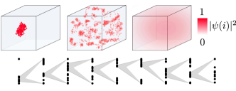
Figure 1: Upper panel - cartoon of a many-body wavefunction in three distinct regimes localized (left), non-ergodic metallic and ergodic states (right). These regimes differ by the ratio of the total number of Fock states, $N$, and the support set $\Omega$, where wavefunction is significant. In a localized state, the volume of the support set, $\Omega$ is finite, or at most logarithmic, so $\Omega/N<\ln(N)/N$. For the non-ergodic metal the support set forms a fractal structure, so $\Omega/N<N^{-\nu}$ with $\nu<1$. In the ergodic phase, the support set scales with the dimension of the Many-Body space, so $\Omega/N\sim 1$ and the probability is uniform. Low panel - the local spectrum (energy levels for which wavefunction is significant on a given site) is similar to the random Cantor set. The full spectrum (left) contains 5000 energy levels forming groups separated by large gaps. Zoom into each group produces similar structure at all energy scales.

The wavefunction in the non-ergodic state can be visualized as hybridization of distant resonances that happen to be very close in energy, see Fig. 1 In contrast to a single body problem, in the many-body one the number of states grows exponentially with the order of the perturbation theory that makes it likely to find weakly coupled very distant but strongly mixed resonances. The states formed by the linear combinations of these resonances form a mini-band that is responsible for delocalization. All energy scales in this mini-band are small and determine the Thouless energy, $E_{Th}$, for the whole system that might become much smaller than average level spacing so that the effective Thouless conductance $g=E_{Th}/\delta\ll 1$ is small and size independent in a wide parameter range. Our numerical results confirm this qualitative picture.

The formation of mini-bands characterized by a small Thouless energy can be viewed as a consequence of weak interaction strength which is nevertheless sufficient for delocalization. This unusual regime is known to occur in critical power-law banded matrices with parametrically small off-diagonal elements $\left\langle H_{nm}^{2}\right\rangle=b^{2}/(n-m)^{2}$ with $b\ll 1$ Cuevas and Kravtsov (2007). In this model the dimensionless conductance turns out to be small $g\sim b$ and size independent.

The conductance that varies by orders of magnitude as a function of parameters but remain size independent distinguishes the many-body localization from localization in three dimension where $g$ is constant only in the critical region where $g\sim 1.$ However, the difference disappears in both localized and ergodic regimes where the conductance becomes a fast function of the size.

The structure of this paper is as follows. In section II the model is introduced and its physical realization as an array of Josephson junctions is explained. A brief description of the numerical methods used in this paper can be found in section III. The theory of fractal local energy spectrum in a multifractal regime is presented in section IV. In this section the correlation function $K(\omega)$ of the local densities of states is introduced and studied in a simple model of multifractality of many-body wave functions that generates a fractal local energy spectrum characterized by the fractal dimension $D_{s}$. A new scaling relationship between this fractal dimension and the fractal dimension $D_{2}$ of many-body wave functions in the Hilbert space is derived. The definition of the many-body Thouless energy and the Thouless conductance is also done in this section in terms of $K(\omega)$ and it is shown that multifractality leads to size-independent Thouless conductance. This theory is tested by the numerical results for $K(\omega)$ in Sec.V. In section VI the many-body Thouless conductance is evaluated numerically and it is shown that it is size-independent in a wide range of parameters of the model. The fractal dimensions $D_{1}$ and $D_{2}$ are numerically evaluated in section VII. The new scaling relationship between the fractal dimensions in the Hilbert and energy space is tested in Sec.VIII. In section IX the $r$-statistics of many-body energy levels is studied and an approximate position of the many-body localization transition in the parameter space is located. In Conclusion the main results of the paper are summarized.

II Model and experimental realization

A simple and physically realizable model is provided by the idealized Josephson junction chain with a high ratio of Josephson, $E_{J}$ and charging energies $E_{C}$, $E_{J}\gg E_{C}$:

$$H= E_{J}\sum_{i=1}^{L}\cos\left(\phi_{i}-\phi_{i+1}\right)+E_{C}\sum_{i=1}^{L}\left(\hat{q}_{i}-n_{i}\right)^{2},$$ (1)

where $\hat{q}$ is the operator conjugated to the phase $\phi_{i}$, $e\,n_{i}$ is the random static offset charge. We will set $E_{C}=1$ which fixes energy units in the following. All the calculations below have been done for the closed loop, $|q_{L+1}\rangle=|q_{1}\rangle$. This geometry is experimentally relevant because it allows to protect the chain from the noise coming from dc lines (see below).

In this system the localization transition is driven by temperature. Unexpectedly, the many-body wavefunction becomes localized at high temperatures $T\geq T_{MBL}$ : $T_{MBL}\sim E_{J}^{2}/E_{C}$ Pino et al. (2016). On the other hand, in the whole range $T\gg E_{J}$ the classical dynamics of the phase is only weakly affected by the Josephson couplings and is almost periodic indicating that the system is non-ergodic in this regime. The low-temperature behavior of a related disordered system has been recently studied in the context of a Bose glass Vogt et al. (2015); Cedergren et al. (2017). For numerical analysis reported here we have restricted the allowed charging states by $-Q\leq q\leq Q$ with $Q=2$. We assume that $n_{i}$ is distributed uniformly in the interval $(-W,W)$ and focus on the regime of relatively strong disorder $W=10$. Note that while in the realistic chain the offset charges $n_{i}$ are completely random, their effective range is $-1/2\leq n\leq 1/2$ because larger $n$ can be eliminated by the shift of $q$. In the model with restricted $-Q\leq q\leq Q$, this is not true and the range of $n$ becomes relevant.

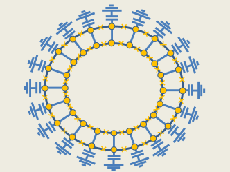
Figure 2: Schematic experimental Josephson-junction array setup in a form of a closed loop.

The sketch of the experimental setup is shown in Fig. 2. First of all we note that in order to control $E_{J}$ one needs to connect the superconducting islands by SQUID loops. The closed geometry significantly reduces the noise coming from environment. Similar physics should hold in an open chain but in order to be decoupled from the environment the dc lines that lead to them should contain superinductance or other decouplers.

In order to ensure $E_{J}<\Delta$ and to neglect thermal quasiparticles we need low transparency junctions. These junctions do not have significant capacitance. It is important that they have small size and do not contain parasitic two-level systems. In order to implement the model Hamiltonian Eq.(1) the experimental setup should have large capacitance to the ground that would dominate ground capacitance. So, the correct setup should contain these capacitors as additional elements (shown in Fig. 2). All these elements should have low loss (in particular low loss tangent of the ground capacitance implies that one should be careful with the choice of dielectric, better to avoid any dielectric in fact).

The ”smoking gun” evidence of the non-ergodic extended phase is the enhanced noise that by far exceeds the one predicted by the Fluctuation-Dissipation Theorem (FDT). Thus studying the noise and comparing it with the linear response at the same frequency one can detect the violation of FDT. Assuming that the effective loss tangent (that takes into account the participation ratio) can be kept at the level of $10^{-4}-10^{-5}$ we expect that one can ignore the dissipation at frequencies higher than 20 kHz. This sets the range for the frequency response $f\sim 10$ kHz.

The main idealization of our approach is the neglect of all excitations except those of the model Hamiltonian Eq.(1). Especially dangerous are the ones associated with the quasiparticles. To avoid thermal quasiparticles we need $T,E_{J}<0.1\,\Delta$. Thus the realistic estimate of parameters of our model are $E_{J}\sim 10-100\,mK$ and $E_{C}\sim 1-10\,mK$.

An important issue is the non-equilibrium quasiparticles that are ubiquitous in the systems considered. Note that the mere presence of the stationary quasiparticle in the island does do any harm. The problem is the motion of quasiparticles between the islands that change the random offset charge. The rate of this motion depends on the experimental setup, it can vary between $1$ kHz Wang et al. (2014) and minutes Bell et al. (2016). In any case it is much lower than the frequency at which the response (noise) should be studied. It can be viewed as a random change of the offset charge configuration, similar to numerical experiments in which we studied quantities averaged over many configurations. The effect of the non-thermal quasiparticles will be exactly to reproduce the averaging in numerical experiments.

III Numerical method

We perform the exact diagonalization of the restricted model (1) and analyze a few states at energies ${E=E_{gs}+\bar{\epsilon}\,\mathfrak{W}}$, where $E_{gs}$ and $\mathfrak{W}$ are the ground-state energy and the many-body band-width. The numerical diagonalization of Hamiltonian Eq. (1) has been done by two methods. In the first one, we have used partial diagonalization to obtain a few eigenstates at a given energy density with ARAPCK’s shift invert mode Lehoucq et al. (1998); Luitz et al. (2015) . In the second one, we have used a full diagonalization to obtain all the eigenstates. The former method allows the computation of system with sizes up to $L=11$, while the last one is only capable of solving sizes up to $L=8$. We will mainly present results for eigenstates at energy $\bar{\epsilon}=0.1$. Partial diagonalization of Many-Body system is more efficient away from the middle of the spectrum than at the band center, where the mean level spacing is much smaller. Thus, the choice of energy density $\bar{\epsilon}=0.1$ allows to reach larger system sizes.

The number of disorder realization of Hamiltonian Eq.1 used to average a given quantity has been chosen to make sensible error bars. Error bars are computed as the standard deviation of the population of measurements given by different realization of the disorder. We notice that smaller values of $E_{J}$ requires larger number of disorder realizations. Thus, for $E_{J}\leq 4$, we have used around $10^{4}$ realizations and for $E_{J}$=14 around $10^{3}$.

Note that at the largest system size $L=8$ attainable for full diagonalization the size of the Hilbert space was $N\sim 10^{6}$, so that together with the number of disorder realizations $\sim 10^{4}$ and 10 different values of $E_{J}$ the computational cost was really enormous.

IV LDoS correlation function and fractality of local energy spectrum.

A central part of this work is to compute the many-body Thouless energy Kravtsov et al. (2015); Serbyn et al. (2016). To this end we employ the correlation function $K(\omega)$ of Local Densities of States (LDoS) between two points $E+\omega/2$ and $E-\omega/2$ in the energy space. It is defined by Cuevas and Kravtsov (2007):

$$K_{E}(\omega)=\frac{{N^{2}}\sum_{\alpha,\beta}\overline{|\psi_{\alpha}(i)|^{2}|\psi_{\beta}(i)|^{2}\delta(E_{\alpha}-E_{-})\delta(E_{\beta}-E_{+})}}{\sum_{\alpha,\beta}\overline{\delta(E_{\alpha}-E_{-})\delta(E_{\beta}-E_{+})}}$$ (2)

where $N$ is the dimension of Hilbert space, $E_{\pm}=E\pm\omega/2$, $\psi_{\alpha}(i)$ is the wavefunction at site $i$ in the Hilbert space of charge quantum numbers, the bar means average over all different charge states and disorder realizations. The denominator in Eq.(2) serves to factor out the effect of level repulsion at small $\omega$ and extract a pure correlation of different wave functions at a site. At larger $\omega$ the level repulsion can be neglected and the factor $N^{2}/\sum_{\alpha,\beta}\overline{\delta(E_{\alpha}-E_{-})\delta(E_{\beta}-E_{+})}$ reduces to $\rho(E)^{-2}$, where $\rho(E)=N^{-1}\sum_{\alpha}\overline{\delta(E-E_{\alpha})}$ is the global density of states.

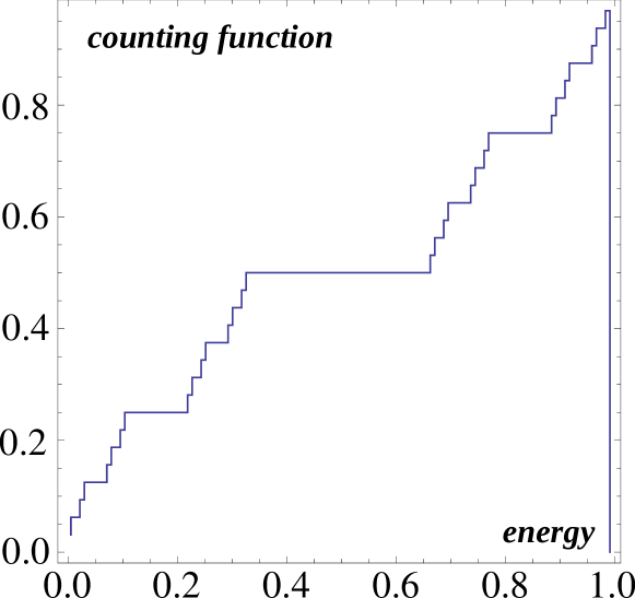
Figure 3: (Color online) Counting function for the standard Cantor set with fractal dimension $D_{s}=\ln 2/\ln 3$. Each new level corresponds to a step in the vertical direction. The plateaus correspond to a gap in the spectrum. There is a middle gap of the width 1/3; in each of the side bands there is its own middle gap of the width 1/9, etc.

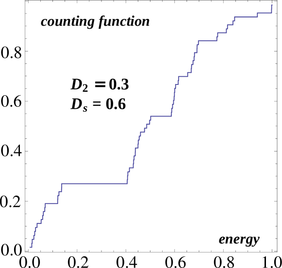
Figure 4: (Color online) Counting function for a random Cantor set, Eq.(3) with $D_{2}=0.3$, generated by statistically independent identically distributed level spacings with the distribution given by Eq.(4) at $D_{s}=0.6$.

For ergodic normalized wave function their overlap is perfect and energy-independent $|\psi_{\alpha}(i)|^{2}\,|\psi_{\beta}(i)|^{2}\sim N^{-2}$, and the correlation function $K(\omega)\sim 1$ is a constant. For localized wave functions it is exponentially small for most of disorder realizations but in rare events which happen with probability $\sim 1/N^{2}$ it is very large $\sim N^{2}$.

For the non-ergodic multifractal wave functions the correlation function $K_{E}(\omega)$ is a power-law in $|\omega|$ which low-energy cutoff is the Thouless energy. This power-law is a signature of fractality of local energy spectrum which can be illustrated by the following simplified model.

In this model we assume Cuevas and Kravtsov (2007) that wave functions are grouped in certain families sharing the same fractal support set in the Hilbert space. Each support set consists of $M\sim N^{D_{2}}$ sites, where $D_{2}$ is its Housedorff dimension of the support set. Since multifractal wave functions are extended over the support set and have vanishingly small amplitude outside it, by normalization their amplitude on a support set is $|\psi|^{2}\sim M^{-1}\sim N^{-D_{2}}$. Under this assumption at $\omega\gg\delta\sim(N\rho(E))^{-1}$ one can represent the correlation function $K(\omega)=\int K_{E}(\omega)\,\rho(E)^{2}\,dE$ as follows:

$$K(\omega)=M^{-2}\sum_{a,b}\delta(\omega-E_{ab}),$$ (3)

where $E_{ab}=E_{a}-E_{b}$ is the difference between energies for the states belonging to the same family which support set includes the observation point $i$ where LDoS is evaluated.

Clearly, the distribution of the level spacings for such states (”local level” spacings) may differ qualitatively from the global level spacing distribution. Indeed, Eq.(3) contains only those levels which states belong to the same family, other states are completely discriminated out. This may lead to large gaps between the local levels inside which levels of other families are situated. These gaps are statistically much more probable than for the global spectrum where all levels are taken into account.

A natural assumption (which will be confirmed by our numerics) is that the fractality in the Hilbert space corresponds to a fractality in the local energy spectrum. In other words, fractality is a property of eigenstates in the ”Hilbert space-local energy spectrum” extension rather than only a spacial property of eigenstates.

A well-known example of a fractal spectrum is the standard Cantor set (see Fig.3). Remarkably, a similar hierarchical structure of gaps can be generated (seeFig.4) in the simple model of statistically independent local level spacings with the power-law probability density identical for all spacings Kravtsov and Scardicchio :

$$P(\Delta)\sim\frac{(E_{{\rm Th}})^{D_{s}}}{\Delta^{1+D_{s}}},\,\,\Delta>E_{{\rm Th}},$$ (4)

where $E_{{\rm Th}}$ gives the low-energy cutoff. The exponent $D_{s}$ is the measure of the fractality of the local energy spectrum, $0<D_{s}<1$.

One can easily calculate $K(\omega)$ in the model described by Eq.(3), where $E_{ab}=\sum_{n=b}^{a}\Delta_{n}$, and each $\Delta_{n}$ is i.i.d. random variable with the power-law distribution Eq.(4):

$$k(t)=M^{-2}\sum_{a,b}^{M}\langle e^{-it\sum_{n=b}^{a}\Delta_{n}}\rangle=M^{-1}\left(2\Re\frac{p(t)}{1-p(t)}+1\right)-2M^{-2}\,\Re\left[\left(1+\frac{p(t)-p(t)^{M}}{(1-p(t))}\right)\,\frac{p(t)}{1-p(t)}\right]$$ (5)

where we introduce the Fourier transforms:

$$k(t) =\int K(\omega)e^{-i\omega t}d\omega$$

$$p(t) =\int P(\Delta)e^{-i\omega t}d\Delta.$$

For any distribution function its Fourier transform $p(0)=1$, $\Re p(t\neq 0)<1$ and $p(t\rightarrow\infty)=0.$ In addition, for the power-law distribution function Eq. (4) one obtains in the region of interest $E_{Th}t\ll 1$:

$$1-p(t)\sim(tE_{Th})^{D_{s}}\ll 1,\;\;\;\;(E_{Th}t\ll 1).$$ (6)

Thus in Eq.(5) there is a small parameter $M^{-1}\ll 1$ and a large parameter $(1-p(t))^{-1}$. Competition between them leads to two different regimes.

If $M(1-p)\gg 1$, or $\omega\ll E_{{\rm Th}}\,N^{D_{2}/D_{s}}$, the term proportional to $M^{-2}$ in Eq.(5) can be neglected. Transforming back to the frequency space we get the power law dependence for $N^{D_{2}/D_{s}}\,E_{{\rm Th}}\lesssim\omega\lesssim E_{{\rm Th}}$:

$$K(\omega)=2M^{-1}\int\Re\frac{p(t)}{1-p(t)}\,e^{i\omega t}\,\frac{dt}{2\pi}\sim\frac{(E_{{\rm Th}})^{-D_{s}}}{M\,\omega^{1-D_{s}}}.$$ (7)

In the opposite limit $M\,(1-p)\ll 1$ the leading in $1-p$ term in Eq.(5) is $1-\frac{M}{3}\,(1-p)$. Thus one obtains a faster decay of $K(\omega)$ for $1\gtrsim\omega\gtrsim E_{{\rm Th}}\,N^{D_{2}/D_{s}}$:

$$K(\omega)=-(M/3)\int\Re(1-p(t))\,e^{i\omega t}\,\frac{dt}{2\pi}\sim\frac{M\,(E_{{\rm Th}})^{D_{s}}}{\omega^{1+D_{s}}}.$$ (8)

Finally, at the smallest $\omega\lesssim E_{{\rm Th}}$ the correlation function $K_{E}(\omega)$, Eq.(2), (as well as $K(\omega)\propto K_{E}(\omega)$) reaches the limit set by the inverse participation ratio $I_{2}(N)=\overline{\sum_{i}|\psi(i)|^{4}}\propto N^{-D_{2}}\sim 1/M$:

$$K_{E}(\omega\rightarrow+0)=c\,N\,I_{2}(N)\sim N^{1-D_{2}}.$$ (9)

The coefficient $c$ is not 1 because of the de Broglie oscillations of random wave functions. For completely random oscillations of real wave functions in the Wigner-Dyson Random Matrix Theory this coefficient is equal to 1/3.

In what follows we use Eq.(9) with $c=1/3$ to define the Thouless energy:

$$K_{E}(\omega=E_{{\rm Th}})=\frac{1}{3}\,N\,I_{2}(N).$$ (10)

Next, we define the Many-Body Thouless conductance:

$$g=\frac{E_{{\rm Th}}}{\rho(E)\,N},$$ (11)

as the ratio of the Thouless energy and the many-body mean level spacing $\delta=(\rho(E)\,N)^{-1}$.

Comparing Eq.(7) with Eq.(10), where $P_{2}(N)=N^{-D_{2}}=M^{-1}$, we conclude that in the non-ergodic multifractal phase the Thouless energy must be proportional to $N^{-1}$, and thus the Many-Body Thouless conductance $g$ should be independent of $N$ just as the conventional single-particle Thouless conductance at the critical point of the Anderson localization transition.

As we will see in the next section, this remarkable property is confirmed numerically in the broad interval of parameters of our model which corresponds to $g$ varying by almost two orders of magnitude as these parameters are changing.

Finally, assuming $E_{{\rm Th}}\propto N^{-1}$ and using $M=N^{D_{2}}$ we find the relationships between the critical exponents that control $K(\omega)$:

$$K(\omega)=\frac{A}{\omega^{\mu}}\sim\frac{N^{\beta}}{\omega^{\mu}}.$$ (12)

For $E_{{\rm Th}}\lesssim\omega\lesssim E_{{\rm Th}}\,N^{D_{2}/D_{s}}$ we obtain from Eq.(7):

$$\beta = D_{s}-D_{2},$$ (13)

$$\mu = 1-D_{s}.$$ (14)

These equation should be compared with the ones for the critical point of the 3D Anderson model, where the standard Chalker’s scaling Chalker (1990) holds:

$$\mu=1-D_{2}.$$ (15)

Thus the standard Chalker’s scaling corresponds to $D_{s}=D_{2}$ which implies that the fractality has the same dimension in the Hilbert space (represented by ”sites” $i$) and in the frequency space.

In general, for $\beta\neq 0$ we have a generalized Chalker’s scaling:

$$\mu+\beta=1-D_{2}.$$ (16)

In the next section we will show that the model considered in this paper corresponds to $\beta>0$ (see Fig. 6).

A special limiting case of vanishing fractality of local energy spectrum corresponds to $D_{s}=1$ in Eq.(4). In this case

$$1-p(t)\sim-C\;it\,\ln(it\,E_{0}),$$

where $C$ and $E_{0}$ are the pre-factor in front of the power-law and its low-$\Delta$ cutoff. In this case Eq.(7) predicts a very slow, logarithmic decrease of the correlation function at $E_{0}\lesssim\omega\lesssim M\,C$:

$$K(\omega)\sim\frac{1}{M\,C\,\ln(\omega/E_{0})}.$$ (17)

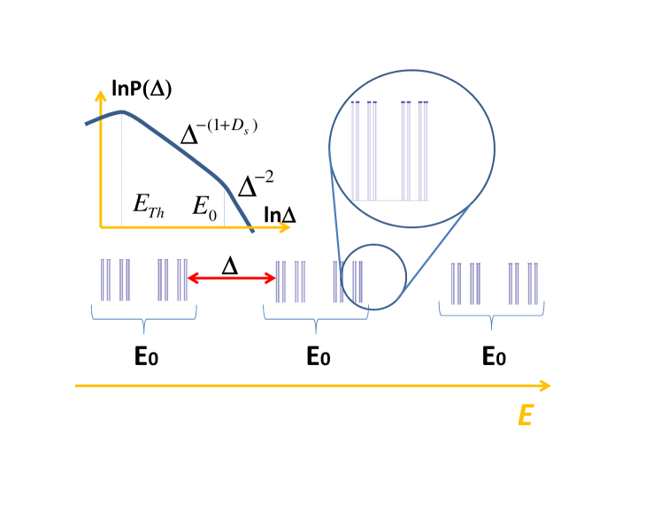
Figure 5: (Color online) Minibands in the local energy spectrum corresponding to Eqs.(7),(20). $E_{0}$ sets the maximal scale of hierarchical structure. ”Cantor sets” of the width $\sim E_{0}$ are separated by the gaps $\Delta\gtrsim E_{0}$ which do not have a hierarchical structure. Inset: probability density of local level spacings.

Eq.(17) applies also in the case where $P(\Delta)$ is given by Eq.(4) with $D_{s}<1$ for $\Delta<E_{0}$ and by

$$P(\Delta)\sim\frac{C}{\Delta^{2}},$$ (18)

for $\Delta>E_{0}$, where $E_{0}>E_{{\rm Th}}$ is some crossover scale that may depend on $N$, e.g. $E_{0}\sim N^{-z}$. In this case the normalization of $P(\Delta)$ (that is still determined by the small $\Delta\sim E_{{\rm Th}}$) requires the constant $C$ to be equal to:

$$C\sim(E_{{\rm Th}})^{D_{s}}\,(E_{0})^{1-D_{s}}.$$ (19)

Comparing Eqs.(17),(19) with Eq.(7) one concludes that in the interval $E_{0}\lesssim\omega\lesssim N^{-\beta}\,(E_{0})^{1-D_{s}}$ the correlation function $K(\omega)$ acquires a ”high-energy plateau” where it depends on $\omega$ very slowly:

$$K(\omega)\sim\frac{(E_{{\rm Th}})^{-D_{s}}}{M\,(E_{0})^{1-D_{s}}}\,\frac{1}{\ln(\omega/E_{0})}\propto\frac{N^{\beta+z\mu}}{\ln(\omega/E_{0})}.$$ (20)

The numerical results for $K(\omega)$ presented in the next section seem to indicate on existence of such a plateau. This result implies that the frcatality of local energy spectrum with hierarchy of mini-bands exists in this model at small energy scales ${E_{{\rm Th}}}\lesssim\omega\lesssim E_{0}$, while the large gaps between ”random Cantor sets” do not show a hierarchical structure (see Fig.5).

V Numerical results for $K(\omega)$.

The results of the numerical computation of $K(\omega)$ are shown in Fig. 6 for the intermediate value of $E_{J}=4$.

The largest size displayed in this figure corresponds to Hilbert space size $N\sim 10^{6}$ and the statistics of $\sim 10^{4}$ samples.

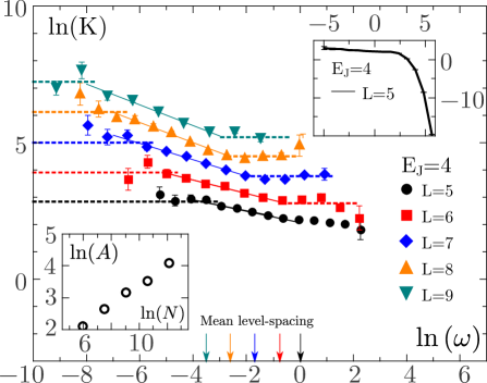
Figure 6: Logarithm of the LDoS correlation function, $\ln K_{E}(\omega)$, as a function of the logarithm of the energy difference $\ln\omega$ in the multifractal regime, $E_{J}=4$. Each data set corresponds to a different system size $L$. The arrows indicate the many-body mean-level spacing, $\delta=(\rho(E)\,N)^{-1}$, for each of the sizes. Partial diagonalization is used to compute $\ln(K_{E})$ with a few eigenstates at the reduced energy $\bar{\epsilon}=0.1$ in the main panel. The solid lines are fits $\ln K_{E}=\ln A-\mu\ln\omega$ that gives $\mu=0.20,\ 0.25,\ 0.30,0.36,\ 0.38$ for $L=5,6,7,8,9$ respectively. The dotted horizontal lines at low frequencies represents $\ln(N\,I_{2}/3)$, where $I_{2}=\sum_{i}\overline{|\psi_{\alpha}(i)|^{4}}$. Intersection of the dotted and solid lines corresponds to $\omega=E_{{\rm Th}}$, see Eq.(10). The horizontal dotted lines at higher frequencies show an approximate ”high-energy plateau”. The frequency $\omega=E_{0}$ at the onset of this plateau corresponds approximately to the global mean level spacing $E_{0}\approx\delta\sim N^{-0.6}$. Inserts: (top) the dependence $\ln(K_{E}(\omega))$ in the whole range of $\omega$ obtained from full diagonalization for $L=5$ and (bottom) the logarithm of the pre-factor $A$ in Eq.(12) as a function of $\ln(N)$.

Two features are remarkable: $K_{E}(\omega)$ has a power law dependence in a wide frequency interval $E_{Th}<\omega<E_{0}$ which is well described by Eq.(12), and the exponents of this power law are non-trivial ($\mu\approx 0.4$, $\beta\approx 0.3$). Using the theory of Sec.IV we may extract the fractal dimensions $D_{2}\approx 0.3$ and $D_{s}\approx 0.6$ in the Hilbert and energy space. The observed power-law and the values of the critical exponents consistent with the theory is a strong argument in favor of the statement that for this choice of parameters of the model ($E_{J}=4$, $E_{C}=1$, $W=10$, $\bar{\epsilon}=0.1$) the system is in the non-ergodic, multifractal phase. The fractal structure of the local energy spectrum implies that in this regime the wavefunction is first spread over a small cluster of close resonances, these resonances are weakly entangled with another cluster further away to form a supercluster, etc. to eventually form a large scale hierarchical structure similar to spin glasses.

The second feature is the ”high-energy plateau” shown by horizontal dotted lines. It is remarkable that the onset of this plateau (or the upper cutoff of the power-law, Eq.(12)) is approximately equal to the global mean level spacing $E_{0}\approx\delta=(\rho(E)\,N)^{-1}$. This scale is much larger than the Thouless energy only because the calculations were done at $\bar{\epsilon}=0.1$ where the mean DoS $\rho(E)\sim 10^{-4}$ is very small. In agreement with the theory of the previous section this implies (see Fig.5) that the hierarchical structure of gaps between mini-bands in the local energy spectrum exists only up to the scale coinciding with the global mean level spacing.

VI Scaling approach of the Many-Body Localization Transition

The data shown in Fig. 6 and similar data for different $E_{J}$ can be used to compute the Thouless energy defined by Eq.(10). In order to avoid direct computation of $K(\omega)$ at low frequencies we used the result for the participation ratio $I_{2}=\overline{\sum_{i}|\psi_{\alpha}(i)|^{4}}$. As explained in Sec.IV, one expects that $K(\omega\rightarrow 0)\rightarrow c\,N\,I_{2}$ where $c\sim 1$. For Gaussian random matrix $c=1/3$, we shall use this value because it agrees very well with the results of the computation at small sizes $L$ for which we were able to compute $K(\omega)$ for small $\omega$ directly. Note that direct computation of $K(\omega)$ at $\omega\rightarrow 0$ is very difficult due to a small number of states with small energy differences. Combining the asymptotic at very small frequencies (shown by dashed horizontal lines in Fig.6) with the power law dependence at $E_{{\rm Th}}<\omega<E_{0}$ (shown by tilted solid line) we determined the crossover frequency $E_{{\rm Th}}$ as the frequency where these two lines intersect. Then we obtain the many-body Thouless conductance $g=E_{{\rm Th}}/\delta$ shown in Fig. 7.

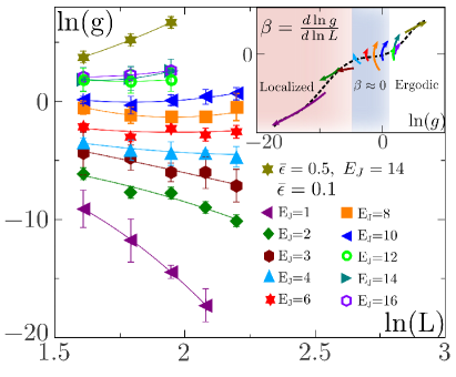
Figure 7: Logarithm of the Thouless conductance, $g=E_{{\rm Th}}/\delta$, as a function of the dimension $N$ of the Hilbert space. The up-most curve in the main panel has been computed in the middle of the band, $\bar{\epsilon}=0.5$. All other curves correspond to the energy $\bar{\epsilon}=0.1$. The insert shows the $\beta(g)=d\ln g/d\ln N$ function computed from these data. The dotted line is a fit of all the $\beta$ functions for different sizes to a 5th order polynomial.

The size dependence of the Thouless conductance displays three distinct regimes. For $E_{J}\lesssim 3$ it decreases exponentially with the system size $L\approx\ln N/\ln 5$ (or as power-law with the dimension $N$ of the Hilbert space), similar to localized regime in conventional single-particle theory. However, the slope of the power-law $N$-dependence decreases as $E_{J}$ increases. The value of $E_{J}$ where the slope vanishes coincides well with the critical value $E_{J}^{(cr)}\approx 3.5$ of the full many-body localization found from the level statistics (see section IX).

In the interval $10\gtrsim E_{J}\gtrsim 4$ the Thouless conductance stays almost constant as $N$ changes by two orders of magnitude. Notice that the decrease of $g(L)$ disappears when $g\sim 10^{-2}$ is very small and it stays $L$-independent in a wide interval of $E_{J}$ where $g(E_{J})$ changes by three orders of magnitude from $\sim 10^{-2}$ to $\sim 10$.

Only at $E_{J}\gtrsim 14$ an exponential increase with the system size $L$ is observed, signaling the appearance of a conventional ergodic state. This increase is still within the error bars for $\bar{\epsilon}=0.1$ but it becomes unquestionable in the band center $\bar{\epsilon}=0.5$.

These three regimes are shown in the inset of Fig.7 where $d\ln g/d\ln N$ is presented as a function of $g$. The appearance of a wide interval of $g$ where $\beta(g)=d\ln g/d\ln N$ is nearly constant is a remarkable feature of our model which allows to make a conclusion about existence of a non-ergodic extended phase of a bad metal, or critical metal, in the Josephson Junction Array model under consideration.

This behavior is in a sharp contrast with that for three-dimensional localization, in which case the conductance varies exponentially with the system size $L$ for small $g$, is a power law in the system size for large $g$, and only in the critical point of the localization transition, where $g\sim 1$, it is $L$-independent. This difference is due to the fact that in three dimensions the probability to find a resonance site within the energy interval $\Delta E$ at a distance $R$ increases as a power of the distance whereas the tunneling amplitude decreases exponentially with $R$. Since conductance at size $L$ is proportional to the tunneling amplitude at this size, at small conductance $g\ll g_{c}\sim 1$ the virtual processes in which the particle hops to the state close in energy in order to cross the sample of size $L$ become improbable. In the many-body localization, the Hilbert space has a local tree structure in which the probability to find a resonance site at large distance increases exponentially and can compensate for exponential decrease of the tunneling amplitude.

VII Fractal dimensions of wave functions in the Hilbert space.

Existence of the intermediate non-ergodic phase for $4\lesssim E_{J}\lesssim 10$ is in a full agreement with the analysis of the wavefunction moments, defined by

$$I_{q}=\sum_{i}\overline{|\psi(i)|^{2q}}.$$ (21)

In a multifractal phase $I_{q}\propto N^{-D_{q}\,(q-1)}$. In a generic case the fractal dimensions:

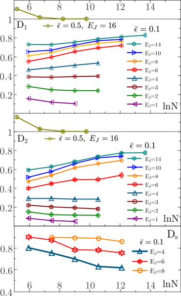
Figure 8: Fractal dimensions ($D_{1},$ $D_{2}$ and $D_{S}$) as a function of logarithm of dimension $N$ of the Hilbert space. Each data set corresponds to a given value of Josephson coupling $E_{J}$. Energy density is $\bar{\epsilon}=0.1$ for all points except one which corresponds to the middle of the spectrum $\bar{\epsilon}=0.5$.

$$D_{q} =-\frac{1}{q-1}\,\left(\frac{d\ln I_{q}}{d\ln N}\right),$$ (22)

depend on the order of the moment $q$. The most popular for applications are $D_{q}$ with $q=2$ and $q=1$ which is understood as the limit of $D_{q}$ as $q\rightarrow 1$.

We computed dimensions $D_{1}$ and $D_{2}$ by employing the discrete, finite-size version of Eq. (22) in which the data for sizes $L+1$ and $L-1$ was used to compute $D_{q}(L)$. In Fig. 8, $D_{q}$ is shown as a function of $\ln N$ (remember that $N\sim 5^{L}$ is the dimension of the Hilbert space) for different Josephson coupling ranging from $E_{J}=1$ to $E_{J}=14$. For very small $E_{J}\leq 2$, the fractal dimensions definitely decrease with the system size increasing and are likely to tend to zero in the limit $N\rightarrow\infty$. This is the signature of the insulating phase. At $E_{J}=3$ the behavior is marginal with a very slow variations within the error bars. Starting from $E_{J}=4$ the increase of fractal dimensions becomes progressively more pronounced, signalling on the delocalized phase. Unfortunately, the evolution is too slow to converge to $N=\infty$ limiting behavior, even at a system size $N\sim 2\times 10^{5}$. This is a typical problem for systems with exponential proliferation of sites which was earlier encountered on a Bethe lattice and Random Regular Graph Altshuler et al. (2016); Tikhonov et al. (2016). It does not allow to determine with absolute certainty the value of $D_{q}(\ln N)$ in the thermodynamical limit. In any case, a clear signature of multifractality is the fact that $D_{1}$ is significantly larger than $D_{2}$ for a wide range of parameters. Together with the size-independence of the Thouless conductance in the interval $4\lesssim E_{J}\lesssim 8$ established in Sec.VI this result sets the lower bound $E_{J}\gtrsim 8$ for the ergodic phase at $\bar{\epsilon}=0.1$. The result in the center of the band $\bar{\epsilon}=0.5$ for $E_{J}=14$ is also consistent with the conclusion of sec.VI that this choice of parameters clearly corresponds to the ergodic phase.

We conclude that both the results on the scaling of Thouless energy and the results of the size dependence of $D_{1}$ and $D_{2}$ show consistently that at $\bar{\epsilon}=0.1$ in the interval $4\lesssim E_{J}\lesssim 8$ the non-ergodic extended, multifractal phase is present in our model. We also note that the multifractality is strong in the range $E_{J}=4$ to $E_{J}=6$, as $D_{1}$ is significantly larger than $D_{2}$.

VIII Relationship between critical exponents

A simple theory of fractality of local energy spectrum presented in Sec.IV suggests a relationship between the exponents $D_{s}=1-\mu$ and $\beta$ describing fractality of the local energy spectrum and the fractal dimension $D_{2}$ of wave functions in the Hilbert space. Combining Eqs.(13),(14) one obtains:

$$D_{s}=1-\mu=\beta+D_{2}.$$ (23)

In the lower panel of Fig.8 we present the data for the fractal dimension $D_{s}=1-\mu$ of local energy spectrum determined from the power-law behavior of $K_{E}(\omega)$. Qualitatively its behavior as a function of $E_{J}$ confirms expectation that multifractality in the Hilbert space and in the energy space are related and both becomes stronger (smaller fractal dimensions) as $E_{J}$ decreases. More quantitative results are presented in Table I.

Table 1: Exponents $\mu,\beta,D_{2}$ and a test of the scaling relationship Eq.(23) between them. The exponents $\mu$ and $D_{2}$ were determined at the largest size of the system for which numerics were available.

$E_{J}$	4	6	8
$\beta$	0.32	0.32	0.29
$D_{2}$	0.23	0.53	0.68
$\beta+D_{2}$	0.55	0.85	0.97
$1-\mu$	0.62	0.76	0.87

Given poor accuracy of $D_{2}$ and $\mu$ which significantly vary with increasing $\ln N$, the fulfilment of the scaling relationship Eq.(23) is very satisfactory.

This is a strong argument in favor of the theory described in Sec.IV which is entirely based on the assumption of multifractality as the simplest form of non-ergodicity in the delocalized phase.

IX Statistic of eigenenergies

Finally we present the results for the so called $r$-statistic, which is the mean ratio of consecutive level spacings $\delta_{n}=E_{i+1}-E_{i}$ in the global spectrum:

$$r=\overline{\min(\delta_{i},\delta_{i+1})/\max(\delta_{i},\delta_{i+1})}.$$

It is a popular measure to distinguish between the MBL localized and extended phases Oganesyan and Huse (2007); Cuevas et al. (2012). For the Wigner-Dyson distribution which corresponds to extreme delocalized, ergodic regime $\left\langle r\right\rangle=0.536$, while for the Poisson distribution expected in the localized phases $\left\langle r\right\rangle=0.386$  Atas et al. (2013). The crossing point of the curves $r_{N}(E_{J})$ for different sizes $N$ marks the many-body localization transition.

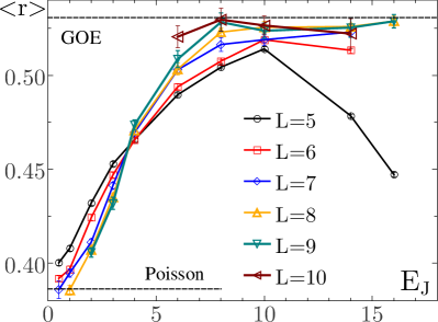
Figure 9: Ratio of minimum and maximum consecutive global level spacings, $r=\overline{\min(\delta_{i},\delta_{i+1})/\max(\delta_{i},\delta_{i+1})}$, for eigenenergies at energy $\bar{\epsilon}=0.1$. Sizes run from $L=5$ to $L=10$, as indicated in the legend. The horizontal lines represent the value of $r$ for the Gaussian Orthogonal ensemble $r_{{\rm WD}}=0.536$ and for the Poisson level statistics $r_{{\rm P}}=0.386$.

Fig. 9, presents $r_{N}(E_{J})$ for the levels at energy $\bar{\epsilon}=0.1$ as a function of $E_{J}$ for several sizes $L=4,5\dots 10$. One observes an apparent crossing point at $E_{J}\approx 3.5$. The spread of curves at $E_{J}>3.5$ clearly indicates to the delocalized phase, while that for $E_{J}<3.5$ shows an insulating behavior only for sizes $L=5,6,7$. For larger sizes the curves are almost coinciding which leaves a possibility that the MBL localization transition is somewhat lower than $E_{J}=3.5$.

An important feature of Fig.9 is that the apparent crossing happens approximately half way from the Poisson to the Wigner-Dyson limits. This is contrary an expectation for the Anderson transition on the hierarchical networks such as Bethe lattice or Random Regular Graph, where the transition point is very close to the Poisson limit. Given a very steep descent of the curves for large $L=7,8,9$ at small $E_{J}$ and the fact that all these curves are almost coinciding, one may expect that the true crossing point corresponds to a value of $r$ much closer to the Poisson limit then that for the apparent crossing point and the critical value for $E_{J}$ is in the interval $2<E_{J}<3$, in agreement with the results of the previous section.

X Conclusion.

Our results confirm existence of the multifractal regime at least in the interval $4\lesssim E_{J}\lesssim 10$ for the model Eq. (1) of the Josephson junction chain. This conclusion is reached by comparing the two sets of data: the correlation function $K(\omega)$ of the local density of states which encodes the property of the local energy spectrum, and the eigenfunction moments $I_{q}$ which contain information on multifractality in the Hilbert space. In this regime both the local energy spectrum and the eigenfunction structure in the Hilbert space are fractal, see Fig. 8. The scaling behavior is characterized by the size-independent many-body Thouless conductance that varies by orders of magnitude as a function of $E_{J}$. This finding is hardly compatible with the single parameter scaling because it leads to a very abnormal $\beta=d\ln g/dL$ function shown in Fig. 7 (see also Ref.Garcia-Mata et al. (2016) for violation of single-parameter scaling on Random Regular Graphs). We would like to mention the soluble 1D model Smith et al. (2017) that exhibits similar behavior due to exact conservation laws. Similar to Josephson junction chain, the number of states per site in this model is larger than 2 which indicates that absence of non-ergodic regime claimed in some previous works Schiulaz et al. (2014); Serbyn and Moore (2016); Serbyn et al. (2016) might be due to the choice of the model with only 2 states per site in 1D chain.

The appearance of a peculiar regime in which $\beta(g)$ function is approximately zero in a wide range of parameters is a clear evidence for the new genuine phase, a “bad” metal. Physically, in this phase one should observe dissipation and transport but the dynamics is slow and thermodynamic equilibrium is never reached. One experimental evidence for such state is a strongly enhanced noise and the violation of FDT. Another evidence is the fractal nature of the local spectra. The observation of the fractal structure of the local spectra is of principal importance. It opens up new direction of investigation of the ”bad metal” phase by various spectral techniques.

Acknowledgment. This work was supported by by ARO grant W911NF-13-1-0431 and Russian Science Foundation 14-42-00044. M. P. acknowledge support from Juan de la Cierva IJCI-2015-23260, MINECO/FEDER Project FIS2015-70856-P, CAM PRICYT Project QUITEMAD+ S2013/ICE-2801 and Proyecto de la Fundacion Seneca 19907/GERM/15.

References

- Anderson (1958) P. W. Anderson, Phys. Rev. 109, 1492 (1958).
- Feher (1959) G. Feher, Phys. Rev. 114, 1219 (1959).
- Basko et al. (2006) D. Basko, I. Aleiner, and B. Altshuler, Annals of Physics 321, 1126 (2006).
- Evers and Mirlin (2008) F. Evers and A. Mirlin, Reviews of Modern Physics 80, 1355 (2008).
- Pino et al. (2016) M. Pino, L. B. Ioffe, and B. L. Altshuler, Proceedings of the National Academy of Sciences 113, 536 (2016).
- Bar Lev and Reichman (2014) Y. Bar Lev and D. R. Reichman, Phys. Rev. B 89, 220201 (2014).
- Luitz et al. (2016) D. J. Luitz, N. Laflorencie, and F. Alet, Phys. Rev. B 93, 060201 (2016).
- Luitz and Bar Lev (2017) D. J. Luitz and Y. Bar Lev, preprint arXiv:1702.03929 (2017).
- Torres-Herrera and Santos (2015) E. J. Torres-Herrera and L. F. Santos, Physical Review B 92, 014208 (2015).
- Schreiber et al. (2015) M. Schreiber, S. S. Hodgman, P. Bordia, H. P. Lüschen, M. H. Fischer, R. Vosk, E. Altman, U. Schneider, and I. Bloch, Science 349, 842 (2015).
- Luschen et al. (2017) H. Luschen, P. Bordia, S. Hodgman, M. Schreiber, S. Sarkar, A. Daley, M. Fischer, E. Altman, I. Bloch, and U. Schneider, Physical Review X 7, 011034 (2017).
- Tamir (2016) I. Tamir, in Talk a CPTGA international workshop strongly disordered and inhomogeneous superconductivity, Grenoble (2016).
- Biroli and Tarzia (2017) G. Biroli and M. Tarzia, arXiv:1706.02655 [cond-mat.stat-mech] (2017).
- De Luca et al. (2014) A. De Luca, B. L. Altshuler, V. E. Kravtsov, and A. Scardicchio, Phys. Rev. Lett. 113, 046806 (2014).
- Altshuler et al. (2016) B. L. Altshuler, E. Cuevas, L. B. Ioffe, and V. E. Kravtsov, Phys. Rev. Lett. 117, 156601 (2016).
- Biroli et al. (2010) G. Biroli, G. Semerjian, and M. Tarzia, Progress of Theoretical Physics Supplement 184, 187 (2010).
- Altshuler et al. (1997) B. L. Altshuler, Y. Gefen, A. Kamenev, and L. S. Levitov, Phys. Rev. Lett. 78, 2803 (1997).
- Tikhonov and Mirlin (2016) K. S. Tikhonov and A. D. Mirlin, Phys. Rev. B 94, 184203 (2016).
- Bertrand and Garcia-Garcia (2016) C. L. Bertrand and A. M. Garcia-Garcia, Phys. Rev. B 94, 144201 (2016).
- Metz and Castillo (2017) F. L. Metz and I. P. Castillo, arXiv:1703.10623 (2017).
- Agarwal et al. (2015) K. Agarwal, S. Gopalakrishnan, M. Knap, M. Müller, and E. Demler, Phys. Rev. Lett. 114, 160401 (2015).
- Gopalakrishnan et al. (2016) S. Gopalakrishnan, K. Agarwal, E. A. Demler, D. A. Huse, and M. Knap, Phys. Rev. B 93, 134206 (2016).
- Serbyn and Moore (2016) M. Serbyn and J. E. Moore, Phys. Rev. B 93, 041424 (2016).
- Deng et al. (2016) X. Deng, B. L. Altshuler, G. V. Shlyapnikov, and L. Santos, Phys. Rev. Lett. 117, 020401 (2016).
- Serbyn et al. (2016) M. Serbyn, Z. Papić, and D. A. Abanin, arXiv preprint arXiv:1610.02389 (2016).
- Cuevas and Kravtsov (2007) E. Cuevas and V. E. Kravtsov, Phys. Rev. B 76, 235119 (2007).
- Vogt et al. (2015) N. Vogt, R. Schäfer, H. Rotzinger, W. Cui, A. Fiebig, A. Shnirman, and A. V. Ustinov, Phys. Rev. B 92, 045435 (2015).
- Cedergren et al. (2017) K. Cedergren, R. Ackroyd, S. Kafanov, N. Vogt, A. Shnirman, and T. Duty, Phys. Rev. Lett. 119, 167701 (2017).
- Wang et al. (2014) C. Wang, Y. Gao, I. Pop, U. Vool, C. Axline, T. Brecht, R. Heeres, L. Frunzio, M. Devoret, G. Catelani, et al., Nature Communications 5 (2014).
- Bell et al. (2016) M. Bell, W. Zhang, L. B. Ioffe, and M. E. Gershenson, Physical review letters 116, 107002 (2016).
- Lehoucq et al. (1998) R. B. Lehoucq, D. C. Sorensen, and C. Yang, ARPACK users’ guide: solution of large-scale eigenvalue problems with implicitly restarted Arnoldi methods, Vol. 6 (Siam, 1998).
- Luitz et al. (2015) D. J. Luitz, N. Laflorencie, and F. Alet, Phys. Rev. B 91, 081103 (2015).
- Kravtsov et al. (2015) V. E. Kravtsov, I. M. Khaymovich, E. Cuevas, and M. Amini, New Journal of Physics 17, 122002 (2015).
- (34) V. Kravtsov and A. Scardicchio, unpublished .
- Chalker (1990) J. Chalker, Physica A: Statistical Mechanics and its Applications 167, 253 (1990).
- Tikhonov et al. (2016) K. S. Tikhonov, A. D. Mirlin, and M. Skvortsov, Physical Review B 94, 220203 (2016).
- Oganesyan and Huse (2007) V. Oganesyan and D. Huse, Physical Review B (Condensed Matter) 75, 155111 (2007).
- Cuevas et al. (2012) E. Cuevas, M. Feigel’man, L. Ioffe, and M. Mezard, Nature Communications 3, 1128 (2012).
- Atas et al. (2013) Y. Y. Atas, E. Bogomolny, O. Giraud, and G. Roux, Phys. Rev. Lett. 110, 084101 (2013).
- Garcia-Mata et al. (2016) I. Garcia-Mata, O. Giraud, B. Georgeot, J. Martin, R. Dubertrand, and G. Lemarie, preprint arXiv:1609.05857 (2016).
- Smith et al. (2017) A. Smith, J. Knolle, D. L. Kovrizhin, and R. Moessner, preprint arXiv:1701.04748 (2017).
- Schiulaz et al. (2014) M. Schiulaz, A. Silva, and M. Mï¿œller, preprint arXiv:1410.4690 (2014).