Regular approximate factorization of a class of matrix-function
with an unstable set of partial indices

G. Mishuris1, S. Rogosin2

1Aberystwyth University, Penglais, SY23 3BZ Aberystwyth, UK

2Belarusian State University, Nezavisimosti Ave., 4, 220030 Minsk, Belarus

Abstract

From the classic work of Gohberg and Krein (1958), it is well known that the set of partial indices of a non-singular matrix function may change depending on the properties of the original matrix. More precisely, it was shown that if the difference between the larger and the smaller partial indices is larger than unity then, in any neighborhood of the original matrix function, there exists another matrix function possessing a different set of partial indices. As a result, the factorization of matrix functions, being an extremely difficult process itself even in the case of the canonical factorization, remains unresolvable or even questionable in the case of a non-stable set of partial indices. Such a situation, in turn, has became an unavoidable obstacle to the application of the factorization technique. This paper sets out to answer a less ambitious question than that of effective factorizing matrix functions with non-stable sets of partial indices, and instead focuses on determining the conditions which, when imposed on the original matrix function, allow to construct another matrix function that exhibits the same partial indices and is close to the original matrix function.

1 Introduction

A given invertible square matrix G∈(π’žβ€‹(ℝ))nΓ—n𝐺superscriptπ’žβ„π‘›π‘›G\in\left({\mathcal{C}}({\mathbb{R}})\right)^{n\times n} is called factorizable if it can be represented in the form

G​(x)=Gβˆ’β€‹(x)​Λ​(x)​G+​(x),𝐺π‘₯superscript𝐺π‘₯Ξ›π‘₯superscript𝐺π‘₯G(x)=G^{-}(x)\Lambda(x)G^{+}(x), (1)

with continuous invertible factors G±​(x),(GΒ±)βˆ’1​(x)superscript𝐺plus-or-minusπ‘₯superscriptsuperscript𝐺plus-or-minus1π‘₯G^{\pm}(x),(G^{\pm})^{-1}(x), possessing analytic continuation into the corresponding half-plane Ξ Β±={z=x+i​y:ImΒ±z<0}superscriptΞ plus-or-minusconditional-set𝑧π‘₯𝑖𝑦plus-or-minusIm𝑧0\Pi^{\pm}=\{z=x+iy:{\mathrm{Im}}\,\pm z<0\}, and

Λ​(x)=diag​((xβˆ’ix+i)Ο°1,…,(xβˆ’ix+i)Ο°n),Ο°1,…,Ο°nβˆˆβ„€.formulae-sequenceΞ›π‘₯diagsuperscriptπ‘₯𝑖π‘₯𝑖subscriptitalic-Ο°1…superscriptπ‘₯𝑖π‘₯𝑖subscriptitalic-ϰ𝑛subscriptitalic-Ο°1…subscriptitalic-ϰ𝑛℀\Lambda(x)={\mathrm{diag}}\,\left(\left(\frac{x-i}{x+i}\right)^{{\varkappa}_{1}},\ldots,\left(\frac{x-i}{x+i}\right)^{{\varkappa}_{n}}\right),\;{\varkappa}_{1},\ldots,{\varkappa}_{n}\in{\mathbb{Z}}. (2)

The representation (1) is called the right (or right-sided) factorization on the real axis. It is also referred to as right continuous factorization. If we have the representation

G​(x)=G+​(x)​Λ​(x)​Gβˆ’β€‹(x),𝐺π‘₯superscript𝐺π‘₯Ξ›π‘₯superscript𝐺π‘₯G(x)=G^{+}(x)\Lambda(x)G^{-}(x), (3)

then it is called the left (or left-sided) factorization. If the right- (or left-) factorization exists, then the integers Ο°1,…,Ο°nsubscriptitalic-Ο°1…subscriptitalic-ϰ𝑛{\varkappa}_{1},\ldots,{\varkappa}_{n}, called the partial indices, are determined uniquely up to their order, e.g. Ο°1β‰₯…β‰₯Ο°nsubscriptitalic-Ο°1…subscriptitalic-ϰ𝑛{\varkappa}_{1}\geq\ldots\geq{\varkappa}_{n}. The factors Gβˆ’superscript𝐺G^{-}, G+superscript𝐺G^{+} are not unique (see, e.g., [16]). In general, the partial indices for the right-factorization and for the left-factorization are not necessarily the same. Throughout this paper we will only deal with the right factorization. The case of the left factorization can be handled analogously.

Several of the general facts on factorization have been presented in the survey paper [20] (see also [7, 14]). In particular, it is well known that the sum of the partial indices is equal to the winding number (or the Cauchy index) of the determinant of the given invertible square matrix G𝐺G:

βˆ‘j=1nΟ°j=Ο°G=w​i​n​dℝ​d​e​t​G​(x)=12β€‹Ο€β€‹βˆ«βˆ’βˆž+∞d​(a​r​g​d​e​t​G​(x)).superscriptsubscript𝑗1𝑛subscriptitalic-ϰ𝑗subscriptitalic-ϰ𝐺𝑀𝑖𝑛subscript𝑑ℝ𝑑𝑒𝑑𝐺π‘₯12πœ‹superscriptsubscriptπ‘‘π‘Žπ‘Ÿπ‘”π‘‘π‘’π‘‘πΊπ‘₯\sum_{j=1}^{n}{\varkappa}_{j}={\varkappa}_{G}=wind_{\mathbb{R}}\;det\,G(x)=\frac{1}{2\pi}\int\limits_{-\infty}^{+\infty}d(arg\,det\,G(x)). (4)

The factorization is called the canonical factorization if all the partial indices are equal to 0, i.e. Ο°1=…=Ο°n=0subscriptitalic-Ο°1…subscriptitalic-ϰ𝑛0{\varkappa}_{1}=\ldots={\varkappa}_{n}=0.

It is said (see, e.g. [8, p. 50]) that a non-singular matrix function G​(x)𝐺π‘₯G(x) has a stable set of partial indices if there exists Ξ΄>0𝛿0\delta>0 such that any matrix function F​(x)𝐹π‘₯F(x) from the δ𝛿\delta-neighbourhood of G​(x)𝐺π‘₯G(x) (i.e. β€–Fβˆ’Gβ€–<Ξ΄norm𝐹𝐺𝛿\|F-G\|<\delta) has the same set of partial indices (right or left). If not, then G​(x)𝐺π‘₯G(x) has an unstable set of partial indices. It has been shown (see [4, 8, 9] and also [15]) that a set of partial indices Ο°1,…,Ο°nsubscriptitalic-Ο°1…subscriptitalic-ϰ𝑛{\varkappa}_{1},\ldots,{\varkappa}_{n} is stable if and only if Ο°1βˆ’Ο°n≀1subscriptitalic-Ο°1subscriptitalic-ϰ𝑛1{\varkappa}_{1}-{\varkappa}_{n}\leq 1.

In the unstable case, a small deformation of the matrix function G​(x)𝐺π‘₯G(x) can lead to changes in the partial indices. More precisely, there exists a sequence of matrix functions Fk​(x)subscriptπΉπ‘˜π‘₯F_{k}(x) that converge to G​(x)𝐺π‘₯G(x), but which has a distinct set of partial indices, i.e.

Fk​(x)=Fkβˆ’β€‹(x)​ΛA​(x)​Fk+​(x),subscriptπΉπ‘˜π‘₯superscriptsubscriptπΉπ‘˜π‘₯subscriptΛ𝐴π‘₯superscriptsubscriptπΉπ‘˜π‘₯F_{k}(x)=F_{k}^{-}(x)\Lambda_{A}(x)F_{k}^{+}(x), (5)

where Ξ›A​(x)≠Λ​(x)subscriptΛ𝐴π‘₯Ξ›π‘₯\Lambda_{A}(x)\not=\Lambda(x).

We note that, in all the known examples illustrating such a situation (see, e.g. [4, 8]), the sequences of the factors Fkβˆ’β€‹(x)superscriptsubscriptπΉπ‘˜π‘₯F_{k}^{-}(x), Fk+​(x)superscriptsubscriptπΉπ‘˜π‘₯F_{k}^{+}(x) do not possess limiting values (as kβ†’βˆžβ†’π‘˜k\to\infty) from the same chosen space as G​(x)𝐺π‘₯G(x). On the contrary, even in the case of unstable partial indices, we can easily construct a sequence of factors Fkβˆ’β€‹(x)superscriptsubscriptπΉπ‘˜π‘₯F_{k}^{-}(x), Fk+​(x)superscriptsubscriptπΉπ‘˜π‘₯F_{k}^{+}(x) in (5) with the same partial indices as the original matrix, i.e. Ξ›A​(x)=Λ​(x)subscriptΛ𝐴π‘₯Ξ›π‘₯\Lambda_{A}(x)=\Lambda(x). Indeed, in a simple example we present the pair Fkβˆ’β€‹(x)=Gβˆ’β€‹(x)+Ξ΅k​Hkβˆ’β€‹(x)superscriptsubscriptπΉπ‘˜π‘₯superscript𝐺π‘₯subscriptπœ€π‘˜subscriptsuperscriptπ»π‘˜π‘₯F_{k}^{-}(x)=G^{-}(x)+\varepsilon_{k}H^{-}_{k}(x), Fk+​(x)=G+​(x)+Ξ΅k​Hk+​(x)superscriptsubscriptπΉπ‘˜π‘₯superscript𝐺π‘₯subscriptπœ€π‘˜subscriptsuperscriptπ»π‘˜π‘₯F_{k}^{+}(x)=G^{+}(x)+\varepsilon_{k}H^{+}_{k}(x), where Hkβˆ“subscriptsuperscript𝐻minus-or-plusπ‘˜H^{\mp}_{k} are arbitrary matrices belonging to the same space as Gβˆ“superscript𝐺minus-or-plusG^{\mp}, such that β€–Hkβˆ“β€–β‰€h0normsubscriptsuperscript𝐻minus-or-plusπ‘˜subscriptβ„Ž0\|H^{\mp}_{k}\|\leq h_{0} and Ξ΅kβ†’0β†’subscriptπœ€π‘˜0\varepsilon_{k}\rightarrow 0 as kβ†’βˆžβ†’π‘˜k\rightarrow\infty.

Let us now consider a matrix function Gβˆˆπ’’β€‹β„‹ΞΌβ€‹(ℝ)nΓ—n𝐺𝒒subscriptβ„‹πœ‡superscriptℝ𝑛𝑛G\in{\mathcal{G}}{\mathcal{H}}_{\mu}({\mathbb{R}})^{n\times n} that possesses a factorization. Any matrix GΞ΅βˆˆπ’’β€‹β„‹ΞΌβ€‹(ℝ)nΓ—nsubscriptπΊπœ€π’’subscriptβ„‹πœ‡superscriptℝ𝑛𝑛G_{\varepsilon}\in{\mathcal{G}}{\mathcal{H}}_{\mu}({\mathbb{R}})^{n\times n} that satisfies the following asymptotic relation

β€–GΡ​(x)βˆ’G​(x)β€–=O​(Ξ΅),Ξ΅β†’0,formulae-sequencenormsubscriptπΊπœ€π‘₯𝐺π‘₯π‘‚πœ€β†’πœ€0\|G_{\varepsilon}(x)-G(x)\|=O(\varepsilon),\;\;\varepsilon\rightarrow 0,

will be called a perturbation of the matrix G𝐺G.

Definition 1.1

Let Gβˆˆπ’’β€‹β„‹ΞΌβ€‹(ℝ)nΓ—n𝐺𝒒subscriptβ„‹πœ‡superscriptℝ𝑛𝑛G\in{\mathcal{G}}{\mathcal{H}}_{\mu}({\mathbb{R}})^{n\times n} be a given factorizable matrix. Its perturbation GΞ΅subscriptπΊπœ€G_{\varepsilon} is considered β€˜regular’, if there exists Ξ΅0>0subscriptπœ€00\varepsilon_{0}>0 such that the matrix GΞ΅subscriptπΊπœ€G_{\varepsilon} possesses a bounded factorization (i.e. |GΡ±​(z)|≀MsuperscriptsubscriptπΊπœ€plus-or-minus𝑧𝑀|G_{\varepsilon}^{\pm}(z)|\leq M for all Ρ∈[0,Ξ΅0)πœ€0subscriptπœ€0\varepsilon\in[0,\varepsilon_{0}) and zβˆˆΞ Β±π‘§superscriptΞ plus-or-minusz\in\Pi^{\pm}). Otherwise the perturbation is considered β€˜singular’.

Lemma 1.1

The partial indices of the regular perturbation GΞ΅subscriptπΊπœ€G_{\varepsilon} are the same as those of G𝐺G.

Proof Let

G​(x)=Gβˆ’β€‹(x)​Λ​(x)​G+​(x),𝐺π‘₯superscript𝐺π‘₯Ξ›π‘₯superscript𝐺π‘₯G(x)=G^{-}(x)\Lambda(x)G^{+}(x),

and GΞ΅subscriptπΊπœ€G_{\varepsilon} be a regular perturbation of G​(x)𝐺π‘₯G(x),

GΡ​(x)=GΞ΅βˆ’β€‹(x)​ΛA​(x)​GΞ΅+​(x)=Gβˆ’β€‹(x)​Λ​(x)​G+​(x)+O​(Ξ΅).subscriptπΊπœ€π‘₯superscriptsubscriptπΊπœ€π‘₯subscriptΛ𝐴π‘₯superscriptsubscriptπΊπœ€π‘₯superscript𝐺π‘₯Ξ›π‘₯superscript𝐺π‘₯π‘‚πœ€G_{\varepsilon}(x)=G_{\varepsilon}^{-}(x)\Lambda_{A}(x)G_{\varepsilon}^{+}(x)=G^{-}(x)\Lambda(x)G^{+}(x)+O(\varepsilon).

Hence

Λ​(x)=(Gβˆ’β€‹(x))βˆ’1​GΞ΅βˆ’β€‹(x)​ΛA​(x)​GΞ΅+​(x)​(G+​(x))βˆ’1+O​(Ξ΅).Ξ›π‘₯superscriptsuperscript𝐺π‘₯1superscriptsubscriptπΊπœ€π‘₯subscriptΛ𝐴π‘₯superscriptsubscriptπΊπœ€π‘₯superscriptsuperscript𝐺π‘₯1π‘‚πœ€\Lambda(x)=\left(G^{-}(x)\right)^{-1}G_{\varepsilon}^{-}(x)\Lambda_{A}(x)G_{\varepsilon}^{+}(x)\left(G^{+}(x)\right)^{-1}+O(\varepsilon).

By taking the limit as Ξ΅β†’+0β†’πœ€0\varepsilon\to+0, we obtain Ξ›A=Ξ›subscriptΛ𝐴Λ\Lambda_{A}=\Lambda due to the uniqueness of the partial indices.

Remark 1.1

If the partial indices of G𝐺G satisfy the condition Ο°m​a​xβˆ’Ο°m​i​n≀1subscriptitalic-Ο°π‘šπ‘Žπ‘₯subscriptitalic-Ο°π‘šπ‘–π‘›1{\varkappa}_{max}-{\varkappa}_{min}\leq 1, then any perturbation of G𝐺G is regular.

Remark 1.2

To highlight the role of the condition of boundedness of the factors, we present here a variant of the classical example of Gohberg and Krein [8, p. 264]. Let us consider the following matrix

G0​(x)=(xβˆ’ix+i00x+ixβˆ’i).subscript𝐺0π‘₯π‘₯𝑖π‘₯𝑖00π‘₯𝑖π‘₯𝑖G_{0}(x)=\left(\begin{array}[]{cc}\frac{x-i}{x+i}&0\\ 0&\frac{x+i}{x-i}\end{array}\right). (6)

It is clear that this matrix possesses a factorization, where G0±​(x)=Isubscriptsuperscript𝐺plus-or-minus0π‘₯𝐼G^{\pm}_{0}(x)=I, Λ​(x)=G0​(x)Ξ›π‘₯subscript𝐺0π‘₯\Lambda(x)=G_{0}(x) and the partial indices Ο°1=1,Ο°2=βˆ’1formulae-sequencesubscriptitalic-Ο°11subscriptitalic-Ο°21{\varkappa}_{1}=1,{\varkappa}_{2}=-1. Consider a slight perturbation of the matrix G0​(x)subscript𝐺0π‘₯G_{0}(x):

GΡ​(x)=(xβˆ’ix+iΞ΅0x+ixβˆ’i),Ξ΅>0.formulae-sequencesubscriptπΊπœ€π‘₯π‘₯𝑖π‘₯π‘–πœ€0π‘₯𝑖π‘₯π‘–πœ€0G_{\varepsilon}(x)=\left(\begin{array}[]{cc}\frac{x-i}{x+i}&\varepsilon\\ 0&\frac{x+i}{x-i}\end{array}\right),\;\;\;\varepsilon>0. (7)

We note that for sufficiently small Ξ΅>0πœ€0\varepsilon>0, the matrices are close to each other, such that

β€–G0​(x)βˆ’GΡ​(x)‖≀Ρ.normsubscript𝐺0π‘₯subscriptπΊπœ€π‘₯πœ€\|G_{0}(x)-G_{\varepsilon}(x)\|\leq\varepsilon.

From the other hand, for all fixed Ξ΅>0πœ€0\varepsilon>0, the matrix GΡ​(x)subscriptπΊπœ€π‘₯G_{\varepsilon}(x) possesses the following factorization with partial indices Ο°1=Ο°2=0subscriptitalic-Ο°1subscriptitalic-Ο°20{\varkappa}_{1}={\varkappa}_{2}=0:

GΡ​(x)=(101Ρ​x+ixβˆ’i1)β‹…Iβ‹…(xβˆ’ix+iΞ΅βˆ’1Ξ΅0).subscriptπΊπœ€π‘₯β‹…101πœ€π‘₯𝑖π‘₯𝑖1𝐼π‘₯𝑖π‘₯π‘–πœ€1πœ€0G_{\varepsilon}(x)=\left(\begin{array}[]{cc}1&0\\ \frac{1}{\varepsilon}\frac{x+i}{x-i}&1\end{array}\right)\cdot I\cdot\left(\begin{array}[]{cc}\frac{x-i}{x+i}&\varepsilon\\ -\frac{1}{\varepsilon}&0\end{array}\right). (8)

For each fixed Ξ΅>0πœ€0\varepsilon>0, the factors in this factorization admit analytic continuations into the corresponding half-plane, where they are bounded. However, these factors are not uniformly bounded for Ρ∈[0,Ξ΅0)πœ€0subscriptπœ€0\varepsilon\in[0,\varepsilon_{0}) for any Ξ΅0>0subscriptπœ€00\varepsilon_{0}>0. Hence GΡ​(x)subscriptπΊπœ€π‘₯G_{\varepsilon}(x) is a singular perturbation of the above diagonal matrix G0​(x)subscript𝐺0π‘₯G_{0}(x) (we denote it by GΞ΅(s)​(x)superscriptsubscriptπΊπœ€π‘ π‘₯G_{\varepsilon}^{(s)}(x)).

This example provides a simple, but not unique, method for the construction of the singular perturbation GΞ΅(s)​(x)superscriptsubscriptπΊπœ€π‘ π‘₯G_{\varepsilon}^{(s)}(x) of any nΓ—n𝑛𝑛n\times n diagonal matrix Λ​(x)=diag​{(xβˆ’ix+i)Ο°1,…,(xβˆ’ix+i)Ο°n}Ξ›π‘₯diagsuperscriptπ‘₯𝑖π‘₯𝑖subscriptitalic-Ο°1…superscriptπ‘₯𝑖π‘₯𝑖subscriptitalic-ϰ𝑛\Lambda(x)={\mathrm{diag}}\left\{\left(\frac{x-i}{x+i}\right)^{\varkappa_{1}},\ldots,\left(\frac{x-i}{x+i}\right)^{\varkappa_{n}}\right\}. Moreover, by replacing Ξ΅πœ€\varepsilon with Ξ΅ksuperscriptπœ€π‘˜\varepsilon^{k} in this procedure, we can construct a singular perturbation for any factorizable matrix G​(x)=Gβˆ’β€‹(x)​Λ​(x)​G+​(x)𝐺π‘₯superscript𝐺π‘₯Ξ›π‘₯superscript𝐺π‘₯G(x)=G^{-}(x)\Lambda(x)G^{+}(x) (see Figure  1),

GΞ΅(s)​(x)=Gβˆ’β€‹(x)​ΛΡ(s)​(x)​G+​(x),superscriptsubscriptπΊπœ€π‘ π‘₯superscript𝐺π‘₯superscriptsubscriptΞ›πœ€π‘ π‘₯superscript𝐺π‘₯G_{\varepsilon}^{(s)}(x)=G^{-}(x)\Lambda_{\varepsilon}^{(s)}(x)G^{+}(x), (9)

which is arbitrarily close to the given matrix G​(x)𝐺π‘₯G(x).

Definition 1.2

Let GΡ​(x)subscriptπΊπœ€π‘₯G_{\varepsilon}(x) be a perturbation of a factorizable matrix function G0​(x)subscript𝐺0π‘₯G_{0}(x) (Ξ΅=0πœ€0\varepsilon=0). If there exists another perturbation GΞ΅βˆ—β€‹(x)superscriptsubscriptπΊπœ€βˆ—π‘₯G_{\varepsilon}^{\ast}(x) satisfying

β€–GΡ​(x)βˆ’GΞ΅βˆ—β€‹(x)β€–=O​(Ξ΅k),Ξ΅β†’0,formulae-sequencenormsubscriptπΊπœ€π‘₯superscriptsubscriptπΊπœ€βˆ—π‘₯𝑂superscriptπœ€π‘˜β†’πœ€0\|G_{\varepsilon}(x)-G_{\varepsilon}^{\ast}(x)\|=O(\varepsilon^{k}),\;\;\varepsilon\rightarrow 0,

then we say that GΞ΅βˆ—superscriptsubscriptπΊπœ€βˆ—G_{\varepsilon}^{\ast} is a β€œk- guided perturbation” of GΞ΅subscriptπΊπœ€G_{\varepsilon}.

It follows from (9) that for each regular perturbation GΡ​(x)subscriptπΊπœ€π‘₯G_{\varepsilon}(x) of the matrix function G0​(x)subscript𝐺0π‘₯G_{0}(x) there exists a singular k-guided perturbation GΞ΅(s)​(x)superscriptsubscriptπΊπœ€π‘ π‘₯G_{\varepsilon}^{(s)}(x) for any kβ‰₯1π‘˜1k\geq 1.

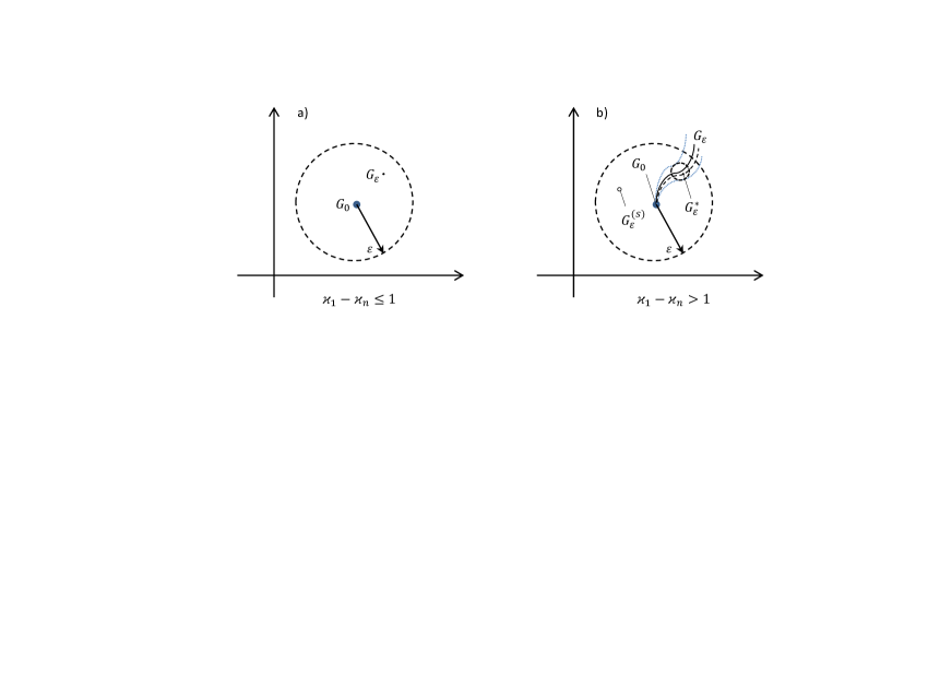
The above mentioned properties are illustrated in Figure 1. In sub-figure a), we show that for any factorizable matrix G0​(x)subscript𝐺0π‘₯G_{0}(x), with a stable set of partial indices, there is a Ξ΅πœ€\varepsilon-neighbourhood containing only regular perturbations. Sub-figure b) illustrates the case of unstable partial indices of G0​(x)subscript𝐺0π‘₯G_{0}(x). Here, the situation is more delicate, as we can see that in each Ξ΅πœ€\varepsilon-neighbourhood of G0​(x)subscript𝐺0π‘₯G_{0}(x) we can find either regular or singular perturbations.

The aim of this paper is to consider the construction of a regular k-guided (k>1π‘˜1k>1) perturbation GΞ΅βˆ—β€‹(x)superscriptsubscriptπΊπœ€βˆ—π‘₯G_{\varepsilon}^{\ast}(x) for a given perturbation GΡ​(x)subscriptπΊπœ€π‘₯G_{\varepsilon}(x) of the matrix function G0​(x)subscript𝐺0π‘₯G_{0}(x), with a known factorization and unstable partial indices. For k=1π‘˜1k=1, this is trivial but gives no practical use.
Refer to caption
Figure 1: Possible types of perturbations, GΞ΅subscriptπΊπœ€G_{\varepsilon}, (β€–GΞ΅βˆ’G0β€–<Ξ΅normsubscriptπΊπœ€subscript𝐺0πœ€\|G_{\varepsilon}-G_{0}\|<\varepsilon), in the cases of stable - a) and unstable - b) sets of partial indices of the matrix-function G0subscript𝐺0G_{0}.

The factorization technique is a powerful tool in solving practical problems [3, 2, 10, 11, 18, 24, 25, 26]), and any approximate factorization will allow a wide range of practical problems to be tackled with some level of accuracy. The establishment of an approximate (see e.g. [1]) or an asymptotic procedure (see [5, 12, 13, 19, 21]) is a challenging problem, since an exact factorization is possible only in a number of special cases (see [20] and references therein). Similarly, the mentioned non-uniqueness of the factorization problem does not prevent it being effectively used in practice. However one needs to be careful in using the approximate factorization in the case of unstable indices, as it may introduce not only quantitative but also qualitative deviation of the approximate solution from the original one. Here, any links between the partial indices of the factorization problem and the particular physical properties of the problem in question are crucial. This question is beyond the scope of this paper.

Below, we discuss whether, and under which conditions, it is possible to find an nΓ—n𝑛𝑛n\times n matrix function GΞ΅βˆ—β€‹(x),xβˆˆβ„superscriptsubscriptπΊπœ€βˆ—π‘₯π‘₯ℝG_{\varepsilon}^{\ast}(x),x\in{\mathbb{R}}, sufficiently close to a given regular perturbation GΡ​(x)subscriptπΊπœ€π‘₯G_{\varepsilon}(x) of the matrix function G0​(x)subscript𝐺0π‘₯G_{0}(x), and possessing an unstable set of partial indices. More exactly, we ask when it is possible to find GΞ΅βˆ—β€‹(x)superscriptsubscriptπΊπœ€βˆ—π‘₯G_{\varepsilon}^{\ast}(x) while preserving the partial indices of GΡ​(x)subscriptπΊπœ€π‘₯G_{\varepsilon}(x)? To reach an answer to this question in the case of unstable partial indices, a new definition of the asymptotic factorization is given and applied. The method, as proposed in [19], [21], is generalized and employed. We find conditions under which our asymptotic procedure is effective, and its properties and details are illustrated by examples. The efficiency of the procedure is also illuminated by numerical results.

The paper is organized as follows: In Sec.  2 we present necessary definitions and notations supplied by necessary basic facts from factorization theory. Next, (Sec.  3) we consider certain perturbations of matrices factorized with unstable partial indices, and describe an algorithm for the construction of an approximate factorization of the perturbed matrices, while preserving the initial partial indices. The conditions for realization of this algorithm are also derived here, which are simply solvability conditions for a certain boundary value problem. We also provide examples where the solvability conditions are satisfied and unsatisfied. We conclude with illustrations of the obtained numerical results and a discussion of their importance in Sec.  4.

2 Asymptotic factorization. Definitions

To proceed, we make some necessary definitions. We denote by ℋμ​(ℝ)nΓ—nsubscriptβ„‹πœ‡superscriptℝ𝑛𝑛{\mathcal{H}}_{\mu}({\mathbb{R}})^{n\times n}, nβˆˆβ„•π‘›β„•n\in\mathbb{N}, the set of bounded matrix functions with locally HΓΆlder-continuous entries, endowed with the norm βˆ₯β‹…βˆ₯ΞΌ\|\cdot\|_{\mu}:

ℋμ​(ℝ)nΓ—n={G=(gi​j):ℝ→ℳnΓ—n:β€–Gβ€–ΞΌ=max1≀i,j≀n⁑‖gi​jβ€–ΞΌ<∞}.subscriptβ„‹πœ‡superscriptℝ𝑛𝑛conditional-set𝐺subscript𝑔𝑖𝑗:→ℝsuperscriptℳ𝑛𝑛subscriptnormπΊπœ‡subscriptformulae-sequence1𝑖𝑗𝑛subscriptnormsubscriptπ‘”π‘–π‘—πœ‡{\mathcal{H}}_{\mu}({\mathbb{R}})^{n\times n}=\left\{G=(g_{ij}):{\mathbb{R}}\rightarrow{\mathcal{M}}^{n\times n}:\|G\|_{\mu}=\max\limits_{1\leq i,j\leq n}\|g_{ij}\|_{\mu}<\infty\right\}. (10)

In this article we consider only matrices of the class 𝒒​ℋμ​(ℝ)nΓ—n𝒒subscriptβ„‹πœ‡superscriptℝ𝑛𝑛{\mathcal{G}}{\mathcal{H}}_{\mu}({\mathbb{R}})^{n\times n}, where 𝒒𝒒{\mathcal{G}} refers to invertible matrices. It should be noted that our method can be also be applied to a wider class of matrix functions.

Below, we give a definition of the asymptotic factorization only in the case of the regular perturbation of a given matrix function, since we lack for the moment a formal procedure which distinguishes between the cases of regular and singular perturbations and as yet have no useful example of the construction of the asymptotic factorization of a singularly perturbed matrix function.

Definition 2.1

Let G0​(x)βˆˆπ’’β€‹β„‹ΞΌβ€‹(ℝ)nΓ—nsubscript𝐺0π‘₯𝒒subscriptβ„‹πœ‡superscriptℝ𝑛𝑛G_{0}(x)\in{\mathcal{G}}{\mathcal{H}}_{\mu}({\mathbb{R}})^{n\times n} be a given factorizable matrix (G0​(x)=G0βˆ’β€‹(x)​Λ​(x)​G0+​(x)subscript𝐺0π‘₯superscriptsubscript𝐺0π‘₯Ξ›π‘₯superscriptsubscript𝐺0π‘₯G_{0}(x)=G_{0}^{-}(x)\Lambda(x)G_{0}^{+}(x)) and GΡ​(x)subscriptπΊπœ€π‘₯G_{\varepsilon}(x) be its regular perturbation. We say that a set of pairs of matrix functions, GΞ΅,mβˆ’β€‹(x)subscriptsuperscriptπΊπœ€π‘šπ‘₯G^{-}_{\varepsilon,m}(x) and GΞ΅,m+​(x)subscriptsuperscriptπΊπœ€π‘šπ‘₯G^{+}_{\varepsilon,m}(x), (m=1,2,…​Nπ‘š12…𝑁m=1,2,\ldots N), and a diagonal matrix Ξ›A​(x)subscriptΛ𝐴π‘₯\Lambda_{A}(x) of the form (2) represent an asymptotic factorization (of the order N) of the matrix function G​(x)βˆˆπ’’β€‹β„‹ΞΌβ€‹(ℝ)nΓ—n𝐺π‘₯𝒒subscriptβ„‹πœ‡superscriptℝ𝑛𝑛G(x)\in{\mathcal{G}}{\mathcal{H}}_{\mu}({\mathbb{R}})^{n\times n} if the following conditions are satisfied:

  1. 1.

    there exists a sequence of functions ΞΈk​(Ξ΅)subscriptπœƒπ‘˜πœ€\theta_{k}(\varepsilon), k=1,2,…​N+1π‘˜12…𝑁1k=1,2,\ldots N+1, that vanishes at the point Ξ΅=0πœ€0\varepsilon=0, such that for any k=1,2,…​Nπ‘˜12…𝑁k=1,2,\ldots N

    ΞΈk+1​(Ξ΅)=o​(ΞΈk​(Ξ΅)),Ξ΅β†’0;formulae-sequencesubscriptπœƒπ‘˜1πœ€π‘œsubscriptπœƒπ‘˜πœ€β†’πœ€0\theta_{k+1}(\varepsilon)=o\big{(}\theta_{k}(\varepsilon)\big{)},\quad\varepsilon\to 0; (11)
  2. 2.

    there exist matrices GΞ΅,mβˆ“β€‹(x)subscriptsuperscript𝐺minus-or-plusπœ€π‘šπ‘₯G^{\mp}_{\varepsilon,m}(x) of the form:

    GΞ΅,mβˆ“β€‹(x)=G0βˆ“β€‹(x)+βˆ‘k=1mΞΈk​(Ξ΅)​HΞ΅,kβˆ“β€‹(x),subscriptsuperscript𝐺minus-or-plusπœ€π‘šπ‘₯superscriptsubscript𝐺0minus-or-plusπ‘₯superscriptsubscriptπ‘˜1π‘šsubscriptπœƒπ‘˜πœ€subscriptsuperscript𝐻minus-or-plusπœ€π‘˜π‘₯G^{\mp}_{\varepsilon,m}(x)={G_{0}}^{\mp}(x)+\sum_{k=1}^{m}\theta_{k}(\varepsilon)H^{\mp}_{\varepsilon,k}(x), (12)
  3. 3.

    there exists Ξ΅0>0subscriptπœ€00\varepsilon_{0}>0 such that the matrices HΞ΅,kβˆ“β€‹(z)subscriptsuperscript𝐻minus-or-plusπœ€π‘˜π‘§H^{\mp}_{\varepsilon,k}(z) are analytical in Ξ βˆ“superscriptΞ minus-or-plus\Pi^{\mp}, respectively, and bounded in ℋμ​(ℝ)nΓ—nsubscriptβ„‹πœ‡superscriptℝ𝑛𝑛{\mathcal{H}}_{\mu}({\mathbb{R}})^{n\times n} uniformly with respect to Ρ∈[0,Ξ΅0)πœ€0subscriptπœ€0\varepsilon\in[0,\varepsilon_{0}),

  4. 4.

    the following estimate is valid for any m=1,2,…​Nπ‘š12…𝑁m=1,2,\ldots N

    G0βˆ’β€‹(x)​Λ​(x)​G0+​(x)βˆ’GΞ΅,mβˆ’β€‹(x)​ΛA​(x)​GΞ΅,m+​(x)=O​(ΞΈm+1​(Ξ΅)),Ξ΅β†’0.formulae-sequencesuperscriptsubscript𝐺0π‘₯Ξ›π‘₯superscriptsubscript𝐺0π‘₯subscriptsuperscriptπΊπœ€π‘šπ‘₯subscriptΛ𝐴π‘₯subscriptsuperscriptπΊπœ€π‘šπ‘₯𝑂subscriptπœƒπ‘š1πœ€β†’πœ€0G_{0}^{-}(x)\Lambda(x)G_{0}^{+}(x)-G^{-}_{\varepsilon,m}(x)\Lambda_{A}(x)G^{+}_{\varepsilon,m}(x)=O\big{(}\theta_{m+1}(\varepsilon)\big{)},\quad\varepsilon\to 0. (13)

The representation

GΞ΅βˆ—β€‹(x)=GΞ΅,Nβˆ’β€‹(x)​ΛA​(x)​GΞ΅,N+​(x),superscriptsubscriptπΊπœ€βˆ—π‘₯subscriptsuperscriptπΊπœ€π‘π‘₯subscriptΛ𝐴π‘₯subscriptsuperscriptπΊπœ€π‘π‘₯G_{\varepsilon}^{\ast}(x)=G^{-}_{\varepsilon,N}(x)\Lambda_{A}(x)G^{+}_{\varepsilon,N}(x), (14)

is called an asymptotic factorization (of order N𝑁N) of the matrix GΡ​(x)subscriptπΊπœ€π‘₯G_{\varepsilon}(x).

We note that conditions (11) and (12) guarantee that the matrices GΞ΅,mβˆ“β€‹(z)subscriptsuperscript𝐺minus-or-plusπœ€π‘šπ‘§{G}^{\mp}_{\varepsilon,m}(z) and (GΞ΅,mβˆ“β€‹(z))βˆ’1superscriptsubscriptsuperscript𝐺minus-or-plusπœ€π‘šπ‘§1({G}^{\mp}_{\varepsilon,m}(z))^{-1} belong to the required class, and thus both terms on the left-hand side of (13) represent two essentially different factorizations. As a simple example of the sequence (11), we could consider ΞΈk​(Ξ΅)=Ξ΅ksubscriptπœƒπ‘˜πœ€superscriptπœ€π‘˜\theta_{k}(\varepsilon)=\varepsilon^{k}.

Some clarifications are required for this definition:

  • β€’

    We are concerned with regular perturbations of the given matrix, i.e. we are looking for representations (12) possessing factors GΞ΅,mβˆ’β€‹(z)subscriptsuperscriptπΊπœ€π‘šπ‘§G^{-}_{\varepsilon,m}(z) and GΞ΅,m+​(z)subscriptsuperscriptπΊπœ€π‘šπ‘§G^{+}_{\varepsilon,m}(z) that are bounded in z𝑧z in the corresponding half-planes, where our choice is motivated purely by applications. In fact, we can replace the boundedness conditions for GΞ΅,mβˆ’β€‹(z)subscriptsuperscriptπΊπœ€π‘šπ‘§G^{-}_{\varepsilon,m}(z) and GΞ΅,m+​(z)subscriptsuperscriptπΊπœ€π‘šπ‘§G^{+}_{\varepsilon,m}(z), by other conditions, such as polynomial growth/decay at infinity.

  • β€’

    The given definition does not demand uniqueness. Indeed, as was demonstrated in the example in [21], which consider the case of stable partial indices, there was no uniqueness, even with the enforcement of additional conditions at infinity.

  • β€’

    The parameter N𝑁N is also involved in the process of asymptotic factorization. In the case when N=βˆžπ‘N=\infty and the series is converging, we can say that the asymptotic factorization becomes the standard factorization, where the factors are defined by their converging series.

  • β€’

    The method used in [21], in the case of stable partial indices, allows to construct for some matrix functions the factors of the factorization as converging asymptotic series, and preserving the partial indices, i.e. Ξ›A​(x)=Λ​(x)subscriptΛ𝐴π‘₯Ξ›π‘₯\Lambda_{A}(x)=\Lambda(x). However, even in this case, no uniqueness can be guaranteed.

  • β€’

    The factors GΞ΅,mβˆ“β€‹(x)superscriptsubscriptπΊπœ€π‘šminus-or-plusπ‘₯G_{\varepsilon,m}^{\mp}(x) in the representation (12) are continuous with respect to Ξ΅β‰₯0πœ€0\varepsilon\geq 0.

  • β€’

    Although the asymptotic factorization is not unique, we can prove, similarly to Lemma 1.1, the uniqueness of the partial indices (Ξ›A​(x)=Λ​(x)subscriptΛ𝐴π‘₯Ξ›π‘₯\Lambda_{A}(x)=\Lambda(x)).

  • β€’

    If an asymptotic factorization of order N>1𝑁1N>1 exists, then the matrix function

    GΞ΅βˆ—β€‹(x)=GΞ΅,Nβˆ’β€‹(z)​Λ​(x)​GΞ΅,N+​(z)superscriptsubscriptπΊπœ€βˆ—π‘₯subscriptsuperscriptπΊπœ€π‘π‘§Ξ›π‘₯subscriptsuperscriptπΊπœ€π‘π‘§G_{\varepsilon}^{\ast}(x)=G^{-}_{\varepsilon,N}(z)\Lambda(x)G^{+}_{\varepsilon,N}(z)

    is an (N+1)𝑁1(N+1)-guided perturbation of the following perturbation GΡ​(x)subscriptπΊπœ€π‘₯G_{\varepsilon}(x) of the matrix G​(x)𝐺π‘₯G(x):

    GΡ​(x)=GΞ΅,1βˆ’β€‹(z)​Λ​(x)​GΞ΅,1+​(z).subscriptπΊπœ€π‘₯subscriptsuperscriptπΊπœ€1𝑧Λπ‘₯subscriptsuperscriptπΊπœ€1𝑧G_{\varepsilon}(x)=G^{-}_{\varepsilon,1}(z)\Lambda(x)G^{+}_{\varepsilon,1}(z).

Although we only consider in this paper the factorization of a matrix function on the real axis, we can tackle in the same way the factorization of matrices defined on any oriented curve ΓΓ\Gamma which divides the complex plane into two domains Dβˆ’superscript𝐷D^{-} and D+superscript𝐷D^{+}, by changing the diagonal entries in Λ​(x)Ξ›π‘₯\Lambda(x) to (xβˆ’t+xβˆ’tβˆ’)Ο°jsuperscriptπ‘₯superscript𝑑π‘₯superscript𝑑subscriptitalic-ϰ𝑗\left(\frac{x-t^{+}}{x-t^{-}}\right)^{{\varkappa}_{j}}, tβˆ“βˆˆDβˆ“superscript𝑑minus-or-plussuperscript𝐷minus-or-plust^{\mp}\in D^{\mp}, or simply to xΟ°jsuperscriptπ‘₯subscriptitalic-ϰ𝑗x^{{\varkappa}_{j}} if 0∈D+0superscript𝐷0\in D^{+}.

Let us now consider a matrix function G0βˆˆπ’’β€‹β„‹ΞΌβ€‹(ℝ)nΓ—nsubscript𝐺0𝒒subscriptβ„‹πœ‡superscriptℝ𝑛𝑛G_{0}\in{\mathcal{G}}{\mathcal{H}}_{\mu}({\mathbb{R}})^{n\times n}, admitting a factorization (1), with unstable partial indices Ο°1,…,Ο°nsubscriptitalic-Ο°1…subscriptitalic-ϰ𝑛{\varkappa}_{1},\ldots,{\varkappa}_{n} (Ο°1β‰₯…β‰₯Ο°nsubscriptitalic-Ο°1…subscriptitalic-ϰ𝑛{\varkappa}_{1}\geq\ldots\geq{\varkappa}_{n}), and its perturbation GΡ​(x)βˆˆπ’’β€‹β„‹ΞΌβ€‹(ℝ)nΓ—nsubscriptπΊπœ€π‘₯𝒒subscriptβ„‹πœ‡superscriptℝ𝑛𝑛G_{\varepsilon}(x)\in{\mathcal{G}}{\mathcal{H}}_{\mu}({\mathbb{R}})^{n\times n}, which depends on a small parameter Ξ΅πœ€\varepsilon such that

GΞ΅(x)|Ξ΅=0=G0(x).G_{\varepsilon}(x)\Bigl{|}_{\varepsilon=0}=G_{0}(x). (15)

Our motivating question is the following: how to distinguish a class of possible perturbations that can be used to construct an asymptotic procedure for the corresponding class of matrices, according to the above definition 2.1, and how to find the conditions under which this procedure can be realized? In the case of stable partial indices, such a type of perturbation and the corresponding asymptotic procedure was proposed in [19, 21] for a class of matrix functions related to certain applied problems. This procedure was shown to be convergent for small values of the parameter Ξ΅πœ€\varepsilon. Here, we extend the technique to the case of unstable partial indices.

3 Asymptotic factorization. Procedure

Let us consider an invertible, bounded, locally HΓΆlder continuous matrix GΡ​(x):ℝ→𝒒​ℋμ​(ℝ)nΓ—n:subscriptπΊπœ€π‘₯→ℝ𝒒subscriptβ„‹πœ‡superscriptℝ𝑛𝑛G_{\varepsilon}(x):{\mathbb{R}}\rightarrow{\mathcal{G}}{\mathcal{H}}_{\mu}({\mathbb{R}})^{n\times n} of the form

GΡ​(x)=G0​(x)+ΞΈ1​(Ξ΅)​NΡ​(x),subscriptπΊπœ€π‘₯subscript𝐺0π‘₯subscriptπœƒ1πœ€subscriptπ‘πœ€π‘₯G_{\varepsilon}(x)=G_{0}(x)+\theta_{1}(\varepsilon)N_{\varepsilon}(x), (16)

where ΞΈ1​(Ξ΅)=o​(1)subscriptπœƒ1πœ€π‘œ1\theta_{1}(\varepsilon)={o}(1) as Ξ΅β†’0β†’πœ€0\varepsilon\to 0 and NΞ΅subscriptπ‘πœ€N_{\varepsilon} is bounded and HΓΆlder continuous on ℝℝ{\mathbb{R}}. We suppose additionally that, when Ξ΅=0πœ€0\varepsilon=0, the matrix G0​(x)subscript𝐺0π‘₯G_{0}(x) possesses a factorization with unstable partial indices (Ο°1βˆ’Ο°nβ‰₯2subscriptitalic-Ο°1subscriptitalic-ϰ𝑛2{\varkappa}_{1}-{\varkappa}_{n}\geq 2), and has factors G0βˆ“β€‹(x)superscriptsubscript𝐺0minus-or-plusπ‘₯G_{0}^{\mp}(x) and (G0βˆ“β€‹(x))Β±1superscriptsuperscriptsubscript𝐺0minus-or-plusπ‘₯plus-or-minus1(G_{0}^{\mp}(x))^{\pm 1}, which admit analytic continuation into the semi-planes Ξ βˆ“superscriptΞ minus-or-plus\Pi^{\mp}, respectively, and which are bounded in Ξ βˆ“Β―=Ξ βˆ“βˆͺℝ¯superscriptΞ minus-or-plussuperscriptΞ minus-or-plusℝ\overline{\Pi^{\mp}}=\Pi^{\mp}\cup{\mathbb{R}}.

We look for an asymptotic factorization of the matrix GΡ​(x)subscriptπΊπœ€π‘₯G_{\varepsilon}(x) of the type (16, which is a regular perturbation of G0​(x)subscript𝐺0π‘₯G_{0}(x), up to some stage of the asymptotic procedure. For simplicity we will consider ΞΈk​(Ξ΅)=Ξ΅ksubscriptπœƒπ‘˜πœ€superscriptπœ€π‘˜\theta_{k}(\varepsilon)=\varepsilon^{k} (see below Remark  3.5, cf. [19, Lemma 3.6]).

3.1 First step of the asymptotic factorization

First, we present the matrix GΡ​(x)subscriptπΊπœ€π‘₯G_{\varepsilon}(x) in the following form:

GΞ΅(x)=(G0βˆ’(x)+Ξ΅N1,Ξ΅βˆ’(x)(Ξ›+(x))βˆ’1)Ξ›(x)Γ—G_{\varepsilon}(x)=\left(G_{0}^{-}(x)+\varepsilon N_{1,\varepsilon}^{-}(x)(\Lambda^{+}(x))^{-1}\right)\Lambda(x)\times (17)
(G0+​(x)+Ρ​(Ξ›βˆ’β€‹(x))βˆ’1​N1,Ξ΅+​(x))+O​(Ξ΅2),superscriptsubscript𝐺0π‘₯πœ€superscriptsuperscriptΞ›π‘₯1superscriptsubscript𝑁1πœ€π‘₯𝑂superscriptπœ€2\left(G_{0}^{+}(x)+\varepsilon(\Lambda^{-}(x))^{-1}N_{1,\varepsilon}^{+}(x)\right)+O(\varepsilon^{2}),

where Ξ›βˆ“β€‹(x)=diag​((xβˆ’ix+i)Ο°1βˆ“,…,(xβˆ’ix+i)Ο°nβˆ“)superscriptΞ›minus-or-plusπ‘₯diagsuperscriptπ‘₯𝑖π‘₯𝑖superscriptsubscriptitalic-Ο°1minus-or-plus…superscriptπ‘₯𝑖π‘₯𝑖superscriptsubscriptitalic-ϰ𝑛minus-or-plus\Lambda^{\mp}(x)={\mathrm{diag}}\,\left(\left(\frac{x-i}{x+i}\right)^{\varkappa_{1}^{\mp}},\ldots{,}\left(\frac{x-i}{x+i}\right)^{\varkappa_{n}^{\mp}}\right), Ο°j+=max⁑{Ο°j,0},Ο°jβˆ’=max⁑{0,βˆ’Ο°j}formulae-sequencesuperscriptsubscriptitalic-ϰ𝑗subscriptitalic-ϰ𝑗0superscriptsubscriptitalic-ϰ𝑗0subscriptitalic-ϰ𝑗\varkappa_{j}^{+}=\max\{\varkappa_{j},0\},\varkappa_{j}^{-}=\max\{0,-\varkappa_{j}\}, and the unknown matrix-functions N1,Ξ΅βˆ“β€‹(x)superscriptsubscript𝑁1πœ€minus-or-plusπ‘₯N_{1,\varepsilon}^{\mp}(x) must be be analytically extended into Ξ βˆ“superscriptΞ minus-or-plus\Pi^{\mp}, together with their inverses, and bounded in Ξ βˆ“Β―Β―superscriptΞ minus-or-plus\overline{\Pi^{\mp}}, respectively. Note that (17) differs from the representation used for the case of stable partial indices (cf., [19], [21]).

Comparing the term with parameter Ξ΅πœ€\varepsilon, we arrive at the following boundary condition for N1,Ξ΅βˆ“superscriptsubscript𝑁1πœ€minus-or-plusN_{1,\varepsilon}^{\mp}:

N1,Ξ΅βˆ’β€‹(x)β€‹Ξ›βˆ’β€‹(x)​G0+​(x)+G0βˆ’β€‹(x)​Λ+​(x)​N1,Ξ΅+​(x)=NΡ​(x).superscriptsubscript𝑁1πœ€π‘₯superscriptΞ›π‘₯superscriptsubscript𝐺0π‘₯superscriptsubscript𝐺0π‘₯superscriptΞ›π‘₯superscriptsubscript𝑁1πœ€π‘₯subscriptπ‘πœ€π‘₯N_{1,\varepsilon}^{-}(x)\Lambda^{-}(x)G_{0}^{+}(x)+G_{0}^{-}(x)\Lambda^{+}(x)N_{1,\varepsilon}^{+}(x)=N_{\varepsilon}(x). (18)

For brevity, we introduce the following notation,

N1,Ξ΅βˆ’~​(x):=(n~1,i​jβˆ’β€‹(z))i​j=(G0βˆ’β€‹(x))βˆ’1​N1,Ξ΅βˆ’β€‹(x),assign~superscriptsubscript𝑁1πœ€π‘₯subscriptsuperscriptsubscript~𝑛1𝑖𝑗𝑧𝑖𝑗superscriptsuperscriptsubscript𝐺0π‘₯1superscriptsubscript𝑁1πœ€π‘₯\widetilde{N_{1,\varepsilon}^{-}}(x):=\left(\tilde{n}_{1,ij}^{-}(z)\right)_{ij}=(G_{0}^{-}(x))^{-1}N_{1,\varepsilon}^{-}(x), (19)
N1,Ξ΅+~​(x):=(n~1,i​j+​(z))i​j=N1,Ξ΅+​(x)​(G0+​(x))βˆ’1,assign~superscriptsubscript𝑁1πœ€π‘₯subscriptsuperscriptsubscript~𝑛1𝑖𝑗𝑧𝑖𝑗superscriptsubscript𝑁1πœ€π‘₯superscriptsuperscriptsubscript𝐺0π‘₯1\widetilde{N_{1,\varepsilon}^{+}}(x):=\left(\tilde{n}_{1,ij}^{+}(z)\right)_{ij}=N_{1,\varepsilon}^{+}(x)(G_{0}^{+}(x))^{-1},
M0,Ρ​(x):=(m0,i​j​(z))i​j=(G0βˆ’β€‹(x))βˆ’1​NΡ​(x)​(G0+​(x))βˆ’1.assignsubscript𝑀0πœ€π‘₯subscriptsubscriptπ‘š0𝑖𝑗𝑧𝑖𝑗superscriptsuperscriptsubscript𝐺0π‘₯1subscriptπ‘πœ€π‘₯superscriptsuperscriptsubscript𝐺0π‘₯1M_{0,\varepsilon}(x):=\left(m_{0,ij}(z)\right)_{ij}=(G_{0}^{-}(x))^{-1}N_{\varepsilon}(x)(G_{0}^{+}(x))^{-1}.

Hence, unknown matrix-functions N1,Ξ΅βˆ“~~superscriptsubscript𝑁1πœ€minus-or-plus\widetilde{N_{1,\varepsilon}^{\mp}} have to satisfy the boundary condition

N1,Ξ΅βˆ’~​(x)β€‹Ξ›βˆ’β€‹(x)+Ξ›+​(x)​N1,Ξ΅+~​(x)=M0,Ρ​(x),xβˆˆβ„.formulae-sequence~superscriptsubscript𝑁1πœ€π‘₯superscriptΞ›π‘₯superscriptΞ›π‘₯~superscriptsubscript𝑁1πœ€π‘₯subscript𝑀0πœ€π‘₯π‘₯ℝ\widetilde{N_{1,\varepsilon}^{-}}(x)\Lambda^{-}(x)+\Lambda^{+}(x)\widetilde{N_{1,\varepsilon}^{+}}(x)=M_{0,\varepsilon}(x),\;x\in{\mathbb{R}}. (20)

In order to determine solvability conditions for this problem and to find a representation for the solution, we present here a few facts from the theory of boundary value problems (see [6],[22]). It is known that any bounded locally HΓΆlder continuous function f:ℝ→ℂ:𝑓→ℝℂf:{\mathbb{R}}\rightarrow{\mathbb{C}} can be uniquely, up to arbitrary constant cβˆˆβ„‚π‘β„‚c\in{\mathbb{C}}, represented as the sum of two functions which are analytic in Ξ βˆ’superscriptΞ \Pi^{-}, Ξ +superscriptΞ \Pi^{+}, an bounded in Ξ βˆ’Β―Β―superscriptΞ \overline{\Pi^{-}}, Ξ +Β―Β―superscriptΞ \overline{\Pi^{+}}, respectively,

f​(x)=((Ξ©0βˆ’β€‹f)​(x)+c)+((Ξ©0+​f)​(x)βˆ’c),𝑓π‘₯superscriptsubscriptΞ©0𝑓π‘₯𝑐superscriptsubscriptΞ©0𝑓π‘₯𝑐f(x)=\left((\Omega_{0}^{-}f)(x)+c\right)+\left((\Omega_{0}^{+}f)(x)-c\right), (21)

where (Ξ©0βˆ“β€‹f)​(z)superscriptsubscriptΞ©0minus-or-plus𝑓𝑧(\Omega_{0}^{\mp}f)(z) is the Cauchy type integral (see [6, p. 52])

(Ξ©0βˆ“β€‹f)​(z)=βˆ“zβˆ’i2​π​iβ€‹βˆ«βˆ’βˆž+∞f​(Ο„)​d​τ(Ο„βˆ’i)​(Ο„βˆ’z),zβˆˆΞ βˆ“.formulae-sequencesuperscriptsubscriptΞ©0minus-or-plus𝑓𝑧minus-or-plus𝑧𝑖2πœ‹π‘–superscriptsubscriptπ‘“πœπ‘‘πœπœπ‘–πœπ‘§π‘§superscriptΞ minus-or-plus(\Omega_{0}^{\mp}f)(z)=\mp\frac{z-i}{2\pi i}\int\limits_{-\infty}^{+\infty}\frac{f(\tau)d\tau}{(\tau-i)(\tau-z)},\;z\in\Pi^{\mp}. (22)

Representation (21), and further formulas, remain valid in the matrix case too. Therefore, the formal solution to (20) has the following form

N1,Ξ΅βˆ’~​(z)=[(Ξ©0βˆ’β€‹M0,Ξ΅)​(z)+C0]​(Ξ›βˆ’β€‹(z))βˆ’1,~superscriptsubscript𝑁1πœ€π‘§delimited-[]superscriptsubscriptΞ©0subscript𝑀0πœ€π‘§superscript𝐢0superscriptsuperscriptΛ𝑧1\widetilde{N_{1,\varepsilon}^{-}}(z)=\left[(\Omega_{0}^{-}M_{0,\varepsilon})(z)+C^{0}\right](\Lambda^{-}(z))^{-1}, (23)
N1,Ξ΅+~​(z)=(Ξ›+​(z))βˆ’1​[(Ξ©0+​M0,Ξ΅)​(z)βˆ’C0],~superscriptsubscript𝑁1πœ€π‘§superscriptsuperscriptΛ𝑧1delimited-[]superscriptsubscriptΞ©0subscript𝑀0πœ€π‘§superscript𝐢0\widetilde{N_{1,\varepsilon}^{+}}(z)=(\Lambda^{+}(z))^{-1}\left[(\Omega_{0}^{+}M_{0,\varepsilon})(z)-C^{0}\right], (24)

where C0superscript𝐢0C^{0} is a constant nΓ—n𝑛𝑛n\times n matrix, which is, in coordinate-wise terms,

{n~1,l​jβˆ’β€‹(z)=(Ξ©0βˆ’β€‹m0,l​j)​(z)+cl​j0, 1≀l≀n,1≀j≀q,n~1,l​jβˆ’β€‹(z)=(zβˆ’iz+i)βˆ’Ο°j​[(Ξ©0βˆ’β€‹m0,l​j)​(z)+cl​j0], 1≀l≀n,q+1≀j≀n;casesformulae-sequenceformulae-sequencesuperscriptsubscript~𝑛1𝑙𝑗𝑧superscriptsubscriptΞ©0subscriptπ‘š0𝑙𝑗𝑧superscriptsubscript𝑐𝑙𝑗01𝑙𝑛1π‘—π‘žmissing-subexpressionformulae-sequenceformulae-sequencesuperscriptsubscript~𝑛1𝑙𝑗𝑧superscript𝑧𝑖𝑧𝑖subscriptitalic-ϰ𝑗delimited-[]superscriptsubscriptΞ©0subscriptπ‘š0𝑙𝑗𝑧superscriptsubscript𝑐𝑙𝑗01π‘™π‘›π‘ž1𝑗𝑛\left\{\begin{array}[]{l}\tilde{n}_{1,lj}^{-}(z)=(\Omega_{0}^{-}m_{0,lj})(z)+c_{lj}^{0},\;1\leq l\leq n,1\leq j\leq q,\\ \\ \tilde{n}_{1,lj}^{-}(z)=\left(\frac{z-i}{z+i}\right)^{-{\varkappa}_{j}}\left[(\Omega_{0}^{-}m_{0,lj})(z)+c_{lj}^{0}\right],\;1\leq l\leq n,q+1\leq j\leq n;\end{array}\right. (25)
{n~1,l​j+​(z)=(z+izβˆ’i)Ο°l​[(Ξ©0+​m0,l​j)​(z)βˆ’cl​j0], 1≀l≀p,1≀j≀n,n~1,l​j+​(z)=(Ξ©0+​m0,l​j)​(z)βˆ’cl​j0,p+1≀l≀n,1≀j≀n.casesformulae-sequenceformulae-sequencesuperscriptsubscript~𝑛1𝑙𝑗𝑧superscript𝑧𝑖𝑧𝑖subscriptitalic-ϰ𝑙delimited-[]superscriptsubscriptΞ©0subscriptπ‘š0𝑙𝑗𝑧superscriptsubscript𝑐𝑙𝑗01𝑙𝑝1𝑗𝑛missing-subexpressionformulae-sequenceformulae-sequencesuperscriptsubscript~𝑛1𝑙𝑗𝑧superscriptsubscriptΞ©0subscriptπ‘š0𝑙𝑗𝑧superscriptsubscript𝑐𝑙𝑗0𝑝1𝑙𝑛1𝑗𝑛\left\{\begin{array}[]{l}\tilde{n}_{1,lj}^{+}(z)=\left(\frac{z+i}{z-i}\right)^{{\varkappa}_{l}}\left[(\Omega_{0}^{+}m_{0,lj})(z)-c_{lj}^{0}\right],\;1\leq l\leq p,1\leq j\leq n,\\ \\ \tilde{n}_{1,lj}^{+}(z)=(\Omega_{0}^{+}m_{0,lj})(z)-c_{lj}^{0},\;p+1\leq l\leq n,1\leq j\leq n.\end{array}\right. (26)

Such a representation gives the bounded solution of the first order asymptotic factorization problem (17), with factors involving analytic matrices N1,Ξ΅βˆ“superscriptsubscript𝑁1πœ€minus-or-plusN_{1,\varepsilon}^{\mp} which are uniquely defined by (19), if and only if certain solvability conditions are satisfied. These conditions simply require that N1,Ξ΅βˆ“~​(z)~superscriptsubscript𝑁1πœ€minus-or-plus𝑧\widetilde{N_{1,\varepsilon}^{\mp}}(z) have no singular points at βˆ“iminus-or-plus𝑖\mp i. Partly, we can use arbitrary constant cl​j0superscriptsubscript𝑐𝑙𝑗0c_{lj}^{0} (the entries of the matrix C0superscript𝐢0C^{0}), but not all the solvability conditions are satisfied by the proper choice of cl​j0superscriptsubscript𝑐𝑙𝑗0c_{lj}^{0}.

3.2 Solvability conditions

Here, we present the necessary and sufficient solvability conditions for boundary value problem (20), which is equivalent to the first step of the asymptotic factorization (see [6, p. 120]).

  • β€’

    if for certain k,q+1≀k≀n,π‘˜π‘ž1π‘˜π‘›k,q+1\leq k\leq n, we have Ο°k=βˆ’1subscriptitalic-Ο°π‘˜1{\varkappa}_{k}=-1, then the boundedness of N1,Ξ΅βˆ’~​(z)~superscriptsubscript𝑁1πœ€π‘§\widetilde{N_{1,\varepsilon}^{-}}(z) at z=βˆ’i𝑧𝑖z=-i follows whenever we choose cl​k0superscriptsubscriptπ‘π‘™π‘˜0c_{lk}^{0} such that

    cl​k0=1Ο€β€‹βˆ«βˆ’βˆž+∞m0,l​k​(Ο„)​d​ττ2+1, 1≀l≀n;formulae-sequencesuperscriptsubscriptπ‘π‘™π‘˜01πœ‹superscriptsubscriptsubscriptπ‘š0π‘™π‘˜πœπ‘‘πœsuperscript𝜏211𝑙𝑛c_{lk}^{0}=\frac{1}{\pi}\int\limits_{-\infty}^{+\infty}\frac{m_{0,lk}(\tau)d\tau}{\tau^{2}+1},\;1\leq l\leq n; (27)
  • β€’

    if for certain k,q+1≀k≀n,π‘˜π‘ž1π‘˜π‘›k,q+1\leq k\leq n, we have Ο°k<βˆ’1subscriptitalic-Ο°π‘˜1{\varkappa}_{k}<-1, then the corresponding cl​k0superscriptsubscriptπ‘π‘™π‘˜0c_{lk}^{0} must be chosen as in (27), and the entries m0,l​k​(Ο„)subscriptπ‘š0π‘™π‘˜πœm_{0,lk}(\tau) have to satisfy conditions

    βˆ«βˆ’βˆž+∞m0,l​k​(Ο„)​d​τ(Ο„+i)r+1=0, 1≀rβ‰€βˆ’Ο°kβˆ’1, 1≀l≀n;formulae-sequenceformulae-sequencesuperscriptsubscriptsubscriptπ‘š0π‘™π‘˜πœπ‘‘πœsuperscriptπœπ‘–π‘Ÿ101π‘Ÿsubscriptitalic-Ο°π‘˜11𝑙𝑛\int\limits_{-\infty}^{+\infty}\frac{m_{0,lk}(\tau)d\tau}{(\tau+i)^{r+1}}=0,\;1\leq r\leq-{\varkappa}_{k}-1,\;1\leq l\leq n; (28)
  • β€’

    if for certain k,1≀k≀p,π‘˜1π‘˜π‘k,1\leq k\leq p, we have Ο°k=1subscriptitalic-Ο°π‘˜1{\varkappa}_{k}=1, then the boundedness of N1,Ξ΅+~​(z)~superscriptsubscript𝑁1πœ€π‘§\widetilde{N_{1,\varepsilon}^{+}}(z) at z=i𝑧𝑖z=i follows whenever we choose ck​j0superscriptsubscriptπ‘π‘˜π‘—0c_{kj}^{0} such that

    ck​j0=0, 1≀j≀n;formulae-sequencesuperscriptsubscriptπ‘π‘˜π‘—001𝑗𝑛c_{kj}^{0}=0,\;1\leq j\leq n; (29)
  • β€’

    if for certain k,1≀k≀p,π‘˜1π‘˜π‘k,1\leq k\leq p, we have Ο°k>1subscriptitalic-Ο°π‘˜1{\varkappa}_{k}>1, then the corresponding ck​j0superscriptsubscriptπ‘π‘˜π‘—0c_{kj}^{0} must be chosen as in (29), and the entries m0,k​j​(Ο„)subscriptπ‘š0π‘˜π‘—πœm_{0,kj}(\tau) have to satisfy conditions

    βˆ«βˆ’βˆž+∞m0,k​j​(Ο„)​d​τ(Ο„βˆ’i)r+1=0, 1≀r≀ϰkβˆ’1, 1≀j≀n;formulae-sequenceformulae-sequencesuperscriptsubscriptsubscriptπ‘š0π‘˜π‘—πœπ‘‘πœsuperscriptπœπ‘–π‘Ÿ101π‘Ÿsubscriptitalic-Ο°π‘˜11𝑗𝑛\int\limits_{-\infty}^{+\infty}\frac{m_{0,kj}(\tau)d\tau}{(\tau-i)^{r+1}}=0,\;1\leq r\leq{\varkappa}_{k}-1,\;1\leq j\leq n; (30)
  • β€’

    if the pair (l,j)𝑙𝑗(l,j) is such that 1≀l≀p,q+1≀j≀nformulae-sequence1π‘™π‘π‘ž1𝑗𝑛1\leq l\leq p,q+1\leq j\leq n, then additional solvability conditions must satisfy

    βˆ«βˆ’βˆž+∞m0,l​j​(Ο„)​d​ττ2+1=0, 1≀l≀p,q+1≀j≀n;formulae-sequenceformulae-sequencesuperscriptsubscriptsubscriptπ‘š0π‘™π‘—πœπ‘‘πœsuperscript𝜏2101π‘™π‘π‘ž1𝑗𝑛\int\limits_{-\infty}^{+\infty}\frac{m_{0,lj}(\tau)d\tau}{\tau^{2}+1}=0,\;1\leq l\leq p,q+1\leq j\leq n; (31)
  • β€’

    if the pair (l,j)𝑙𝑗(l,j) is such that either 1≀l≀n,1≀j≀qformulae-sequence1𝑙𝑛1π‘—π‘ž1\leq l\leq n,1\leq j\leq q, or p+1≀l≀n,1≀j≀nformulae-sequence𝑝1𝑙𝑛1𝑗𝑛p+1\leq l\leq n,1\leq j\leq n, then we have no condition on the entries m0,l​j​(Ο„)subscriptπ‘š0π‘™π‘—πœm_{0,lj}(\tau); the corresponding constants cl​j0superscriptsubscript𝑐𝑙𝑗0c_{lj}^{0} can take arbitrary value.

Theorem 3.1

Formula (17) gives the first order bounded asymptotic factorization for all Ξ΅πœ€\varepsilon smaller than a certain positive Ξ΅1subscriptπœ€1\varepsilon_{1} if ant only if the solvability conditions (28), (30), (31) are satisfied, and the constants ci​j0superscriptsubscript𝑐𝑖𝑗0c_{ij}^{0} are chosen accordingly.

Proof If the conditions of the theorem are satisfied, then the matrix functions N1,Ξ΅βˆ“~​(z)~superscriptsubscript𝑁1πœ€minus-or-plus𝑧\widetilde{N_{1,\varepsilon}^{\mp}}(z) give a bounded solution to the problem (20). Moreover, the matrices N1,Ξ΅βˆ’~​(z)β€‹Ξ›βˆ’β€‹(z)~superscriptsubscript𝑁1πœ€π‘§superscriptΛ𝑧\widetilde{N_{1,\varepsilon}^{-}}(z)\Lambda^{-}(z), Ξ›+​(z)​N1,Ξ΅+~​(z)superscriptΛ𝑧~superscriptsubscript𝑁1πœ€π‘§\Lambda^{+}(z)\widetilde{N_{1,\varepsilon}^{+}}(z) are bounded in the neighbourhoods of z=βˆ’i𝑧𝑖z=-i, z=i𝑧𝑖z=i, respectively. By choosing sufficiently small Ξ΅1>0subscriptπœ€10\varepsilon_{1}>0, we can guarantee that the matrix functions G0βˆ’β€‹(z)+Ρ​N1,Ξ΅βˆ’β€‹(z)​(Ξ›+​(z))βˆ’1superscriptsubscript𝐺0π‘§πœ€superscriptsubscript𝑁1πœ€π‘§superscriptsuperscriptΛ𝑧1G_{0}^{-}(z)+\varepsilon N_{1,\varepsilon}^{-}(z)(\Lambda^{+}(z))^{-1}, G0+​(z)+Ρ​(Ξ›βˆ’β€‹(z))βˆ’1​N1,Ξ΅+​(z)superscriptsubscript𝐺0π‘§πœ€superscriptsuperscriptΛ𝑧1superscriptsubscript𝑁1πœ€π‘§G_{0}^{+}(z)+\varepsilon(\Lambda^{-}(z))^{-1}N_{1,\varepsilon}^{+}(z) are invertible in the corresponding semi-planes. Thus, for Ρ∈[0,Ξ΅1)πœ€0subscriptπœ€1\varepsilon\in[0,\varepsilon_{1}), formula (17) gives the first order bounded asymptotic factorization.

To demonstrate the necessity of the theorem’s conditions, we suppose that formula (17) gives the first order bounded asymptotic factorization. Then the matrix functions N1,Ξ΅βˆ“β€‹(z)superscriptsubscript𝑁1πœ€minus-or-plus𝑧{N_{1,\varepsilon}^{\mp}}(z) have to satisfy boundary condition (18), being analytically extended into Ξ βˆ“superscriptΞ minus-or-plus\Pi^{\mp} together with their inverses, and bounded in Ξ βˆ“Β―Β―superscriptΞ minus-or-plus\overline{\Pi^{\mp}}, respectively. The boundary value problem (18) is equivalent to (20), and for invertibility of matrices N1,Ξ΅βˆ“β€‹(z)superscriptsubscript𝑁1πœ€minus-or-plus𝑧{N_{1,\varepsilon}^{\mp}}(z) we must, in particular, have boundedness of the matrix functions (23), (24) in the neighbourhoods of z=βˆ’i𝑧𝑖z=-i, z=i𝑧𝑖z=i, respectively. The latter leads to the necessity of the conditions of the theorem.

Remark 3.1

The numbers of solvability conditions and conditions on the choice of the constants satisfy the following relations.

  • β€’

    The number of solvability conditions is given by

    βˆ‘j=q+1n(βˆ’Ο°jβˆ’1)​n+βˆ‘i=1p(Ο°iβˆ’1)​n+(nβˆ’q)​p.superscriptsubscriptπ‘—π‘ž1𝑛subscriptitalic-ϰ𝑗1𝑛superscriptsubscript𝑖1𝑝subscriptitalic-ϰ𝑖1π‘›π‘›π‘žπ‘\sum\limits_{j=q+1}^{n}(-{\varkappa}_{j}-1)n+\sum\limits_{i=1}^{p}({\varkappa}_{i}-1)n+(n-q)p. (32)
  • β€’

    (nβˆ’q)​nπ‘›π‘žπ‘›(n-q)n constants ci​j0superscriptsubscript𝑐𝑖𝑗0c_{ij}^{0} are chosen according to (27) and n​p𝑛𝑝np constants ci​j0superscriptsubscript𝑐𝑖𝑗0c_{ij}^{0} are equal to 0, as in (29). In the (nβˆ’q)​pπ‘›π‘žπ‘(n-q)p cases described in (31) these choices of the constants ci​j0superscriptsubscript𝑐𝑖𝑗0c_{ij}^{0} must coincide.

  • β€’

    n​(nβˆ’p+q)π‘›π‘›π‘π‘žn(n-p+q) constants ci​j0superscriptsubscript𝑐𝑖𝑗0c_{ij}^{0} can be chosen arbitrarily.

Remark 3.2

The obtained result can be interpreted in the following manner. Let the matrix function GΡ​(x)subscriptπΊπœ€π‘₯G_{\varepsilon}(x) be a perturbation of G0​(x)subscript𝐺0π‘₯G_{0}(x). Then, in particular, GΡ​(x)subscriptπΊπœ€π‘₯G_{\varepsilon}(x) is in the Ξ΅πœ€\varepsilon-neighbourhood of G0​(x)subscript𝐺0π‘₯G_{0}(x) (see Figure  1 a)). If the matrix GΡ​(x)subscriptπΊπœ€π‘₯G_{\varepsilon}(x) satisfies the above solvability conditions, then there exists for all sufficiently small Ξ΅πœ€\varepsilon the matrix

GΞ΅βˆ—β€‹(x)=(G0βˆ’β€‹(x)+Ρ​N1,Ξ΅βˆ’β€‹(x)​(Ξ›+​(x))βˆ’1)​Λ​(x)​(G0+​(x)+Ρ​(Ξ›βˆ’β€‹(x))βˆ’1​N1,Ξ΅+​(x)),superscriptsubscriptπΊπœ€βˆ—π‘₯superscriptsubscript𝐺0π‘₯πœ€superscriptsubscript𝑁1πœ€π‘₯superscriptsuperscriptΞ›π‘₯1Ξ›π‘₯superscriptsubscript𝐺0π‘₯πœ€superscriptsuperscriptΞ›π‘₯1superscriptsubscript𝑁1πœ€π‘₯G_{\varepsilon}^{\ast}(x)=\left(G_{0}^{-}(x)+\varepsilon N_{1,\varepsilon}^{-}(x)(\Lambda^{+}(x))^{-1}\right)\Lambda(x)\left(G_{0}^{+}(x)+\varepsilon(\Lambda^{-}(x))^{-1}N_{1,\varepsilon}^{+}(x)\right), (33)

which possesses a factorization with the same unstable set of partial indices as G0​(x)subscript𝐺0π‘₯G_{0}(x). The matrix GΞ΅βˆ—β€‹(x)superscriptsubscriptπΊπœ€βˆ—π‘₯G_{\varepsilon}^{\ast}(x) is in the Ξ΅2superscriptπœ€2\varepsilon^{2}-neighbourhood of GΡ​(x)subscriptπΊπœ€π‘₯G_{\varepsilon}(x) (see Figure 1 b)). This means that for each point of linear manifold of the matrices GΡ​(x)subscriptπΊπœ€π‘₯G_{\varepsilon}(x), as defined by (17), which satisfies the solvability conditions, there exists a point (matrix GΞ΅βˆ—β€‹(x)superscriptsubscriptπΊπœ€βˆ—π‘₯G_{\varepsilon}^{\ast}(x)) in its Ξ΅2superscriptπœ€2\varepsilon^{2}-neighbourhood which preserves the initial partial indices, i.e. according to Definition  1.2, the latter matrix is the regular 2-guided perturbation.

3.3 Further steps of the asymptotic factorization

Let the solvability conditions be satisfied and the constants ci​j0superscriptsubscript𝑐𝑖𝑗0c_{ij}^{0} chosen accordingly. By solving the corresponding boundary value problems we can refine the first order factorization up to the rπ‘Ÿr-th step of the factorization using the representation

GΞ΅(x)=(G0βˆ’(x)+Ξ΅N1,Ξ΅βˆ’(x)(Ξ›+(x))βˆ’1+…+Ξ΅rNr,Ξ΅βˆ’(x)(Ξ›+(x))βˆ’1)Ξ›(x)Γ—G_{\varepsilon}(x)=\left(G_{0}^{-}(x)+\varepsilon N_{1,\varepsilon}^{-}(x)(\Lambda^{+}(x))^{-1}+\ldots+\varepsilon^{r}N_{r,\varepsilon}^{-}(x)(\Lambda^{+}(x))^{-1}\right)\Lambda(x)\times (34)
Γ—(G0+​(x)+Ρ​(Ξ›βˆ’β€‹(x))βˆ’1​N1,Ξ΅+​(x)+…+Ξ΅r​(Ξ›βˆ’β€‹(x))βˆ’1​Nr,Ξ΅+​(x))+O​(Ξ΅r+1),absentsuperscriptsubscript𝐺0π‘₯πœ€superscriptsuperscriptΞ›π‘₯1superscriptsubscript𝑁1πœ€π‘₯…superscriptπœ€π‘ŸsuperscriptsuperscriptΞ›π‘₯1superscriptsubscriptπ‘π‘Ÿπœ€π‘₯𝑂superscriptπœ€π‘Ÿ1\times\left(G_{0}^{+}(x)+\varepsilon(\Lambda^{-}(x))^{-1}N_{1,\varepsilon}^{+}(x)+\ldots+\varepsilon^{r}(\Lambda^{-}(x))^{-1}N_{r,\varepsilon}^{+}(x)\right)+O(\varepsilon^{r+1}),

which leads to the boundary value problem

Nr,Ξ΅βˆ’~​(x)β€‹Ξ›βˆ’β€‹(x)+Ξ›+​(x)​Nr,Ξ΅+~​(x)=Mrβˆ’1,Ρ​(x),xβˆˆβ„,formulae-sequence~superscriptsubscriptπ‘π‘Ÿπœ€π‘₯superscriptΞ›π‘₯superscriptΞ›π‘₯~superscriptsubscriptπ‘π‘Ÿπœ€π‘₯subscriptπ‘€π‘Ÿ1πœ€π‘₯π‘₯ℝ\widetilde{N_{r,\varepsilon}^{-}}(x)\Lambda^{-}(x)+\Lambda^{+}(x)\widetilde{N_{r,\varepsilon}^{+}}(x)=M_{r-1,\varepsilon}(x),\;x\in{\mathbb{R}}, (35)
Nr,Ξ΅βˆ’~​(x):=(G0βˆ’β€‹(x))βˆ’1​Nr,Ξ΅βˆ’β€‹(x),Nr,Ξ΅+~​(x):=Nr,Ξ΅+​(x)​(G0+​(x))βˆ’1,formulae-sequenceassign~superscriptsubscriptπ‘π‘Ÿπœ€π‘₯superscriptsuperscriptsubscript𝐺0π‘₯1superscriptsubscriptπ‘π‘Ÿπœ€π‘₯assign~superscriptsubscriptπ‘π‘Ÿπœ€π‘₯superscriptsubscriptπ‘π‘Ÿπœ€π‘₯superscriptsuperscriptsubscript𝐺0π‘₯1\widetilde{N_{r,\varepsilon}^{-}}(x):=(G_{0}^{-}(x))^{-1}N_{r,\varepsilon}^{-}(x),\;\widetilde{N_{r,\varepsilon}^{+}}(x):=N_{r,\varepsilon}^{+}(x)(G_{0}^{+}(x))^{-1}, (36)
Mrβˆ’1,Ρ​(x):=βˆ’(G0βˆ’β€‹(x))βˆ’1​[N1,Ξ΅βˆ’β€‹(x)​Nrβˆ’1,Ξ΅+​(x)+…+Nrβˆ’1,Ξ΅βˆ’β€‹(x)​N1,Ξ΅+​(x)]​(G0+​(x))βˆ’1.assignsubscriptπ‘€π‘Ÿ1πœ€π‘₯superscriptsuperscriptsubscript𝐺0π‘₯1delimited-[]superscriptsubscript𝑁1πœ€π‘₯superscriptsubscriptπ‘π‘Ÿ1πœ€π‘₯…superscriptsubscriptπ‘π‘Ÿ1πœ€π‘₯superscriptsubscript𝑁1πœ€π‘₯superscriptsuperscriptsubscript𝐺0π‘₯1M_{r-1,\varepsilon}(x):=-(G_{0}^{-}(x))^{-1}\left[N_{1,\varepsilon}^{-}(x)N_{r-1,\varepsilon}^{+}(x)+\ldots+N_{r-1,\varepsilon}^{-}(x)N_{1,\varepsilon}^{+}(x)\right](G_{0}^{+}(x))^{-1}.

The formal solution to problem (35) can be presented as

Nr,Ξ΅βˆ’~​(z)=[(Ξ©0βˆ’β€‹Mrβˆ’1,Ξ΅)​(z)+Crβˆ’1]​(Ξ›βˆ’β€‹(z))βˆ’1,~superscriptsubscriptπ‘π‘Ÿπœ€π‘§delimited-[]superscriptsubscriptΞ©0subscriptπ‘€π‘Ÿ1πœ€π‘§superscriptπΆπ‘Ÿ1superscriptsuperscriptΛ𝑧1\widetilde{N_{r,\varepsilon}^{-}}(z)=\left[(\Omega_{0}^{-}M_{r-1,\varepsilon})(z)+C^{r-1}\right](\Lambda^{-}(z))^{-1}, (37)
Nr,Ξ΅+~​(z)=(Ξ›+​(z))βˆ’1​[(Ξ©0+​Mrβˆ’1,Ξ΅)​(z)βˆ’Crβˆ’1],~superscriptsubscriptπ‘π‘Ÿπœ€π‘§superscriptsuperscriptΛ𝑧1delimited-[]superscriptsubscriptΞ©0subscriptπ‘€π‘Ÿ1πœ€π‘§superscriptπΆπ‘Ÿ1\widetilde{N_{r,\varepsilon}^{+}}(z)=(\Lambda^{+}(z))^{-1}\left[(\Omega_{0}^{+}M_{r-1,\varepsilon})(z)-C^{r-1}\right], (38)

which features a new constant matrix Crβˆ’1superscriptπΆπ‘Ÿ1C^{r-1}. It becomes the solution for the considered class if and only if the solvability conditions (27)-(31) are satisfied (in this case we replace the functions m0,i​j​(x)subscriptπ‘š0𝑖𝑗π‘₯m_{0,ij}(x) with the functions mrβˆ’1,i​j​(x)subscriptπ‘šπ‘Ÿ1𝑖𝑗π‘₯m_{r-1,ij}(x), and the constants ci​j0subscriptsuperscript𝑐0𝑖𝑗c^{0}_{ij} with the constants ci​jrβˆ’1subscriptsuperscriptπ‘π‘Ÿ1𝑖𝑗c^{r-1}_{ij}), while the constants ci​jrβˆ’1subscriptsuperscriptπ‘π‘Ÿ1𝑖𝑗c^{r-1}_{ij} are chosen accordingly.

If at a certain step r=N+1π‘Ÿπ‘1r=N+1, at least one solvability condition fails, then the procedure for the the asymptotic factorization is stopped at this point.

Remark 3.3

In this case, we summarize the situation as follows. Let the matrix function GΡ​(x)subscriptπΊπœ€π‘₯G_{\varepsilon}(x) be a regular perturbation of G0​(x)subscript𝐺0π‘₯G_{0}(x). In particular, (as for N=1𝑁1N=1) GΡ​(x)subscriptπΊπœ€π‘₯G_{\varepsilon}(x) is in the Ξ΅πœ€\varepsilon-neighbourhood of G0​(x)subscript𝐺0π‘₯G_{0}(x). If the matrix function GΡ​(x)subscriptπΊπœ€π‘₯G_{\varepsilon}(x) satisfies the above solvability conditions at each step r,1≀r≀N,π‘Ÿ1π‘Ÿπ‘r,1\leq r\leq N, then for all sufficiently small Ξ΅πœ€\varepsilon there exists a matrix

GN,Ξ΅βˆ—β€‹(x)=(G0βˆ’β€‹(x)+βˆ‘r=1NΞ΅r​Nr,Ξ΅βˆ’β€‹(x)​(Ξ›+​(x))βˆ’1)​Λ​(x)​(G0+​(x)+βˆ‘r=1NΞ΅r​(Ξ›βˆ’β€‹(x))βˆ’1​Nr,Ξ΅+​(x)),superscriptsubscriptπΊπ‘πœ€βˆ—π‘₯superscriptsubscript𝐺0π‘₯superscriptsubscriptπ‘Ÿ1𝑁superscriptπœ€π‘Ÿsuperscriptsubscriptπ‘π‘Ÿπœ€π‘₯superscriptsuperscriptΞ›π‘₯1Ξ›π‘₯superscriptsubscript𝐺0π‘₯superscriptsubscriptπ‘Ÿ1𝑁superscriptπœ€π‘ŸsuperscriptsuperscriptΞ›π‘₯1superscriptsubscriptπ‘π‘Ÿπœ€π‘₯G_{N,\varepsilon}^{\ast}(x)=(G_{0}^{-}(x)+\sum\limits_{r=1}^{N}\varepsilon^{r}N_{r,\varepsilon}^{-}(x)(\Lambda^{+}(x))^{-1})\Lambda(x)(G_{0}^{+}(x)+\sum\limits_{r=1}^{N}\varepsilon^{r}(\Lambda^{-}(x))^{-1}N_{r,\varepsilon}^{+}(x)), (39)

which possesses a factorization with the same set of unstable partial indices as G0​(x)subscript𝐺0π‘₯G_{0}(x). The matrix GN,Ξ΅βˆ—β€‹(x)superscriptsubscriptπΊπ‘πœ€βˆ—π‘₯G_{N,\varepsilon}^{\ast}(x) is in the Ξ΅N+1superscriptπœ€π‘1\varepsilon^{N+1}-neighbourhood of GΡ​(x)subscriptπΊπœ€π‘₯G_{\varepsilon}(x). This means that for each point of linear manifold of the matrices GΡ​(x)subscriptπΊπœ€π‘₯G_{\varepsilon}(x) that satisfies the solvability conditions, there exists an (N+1)𝑁1(N+1)-guided perturbation. Thus, with a larger number of steps we can proceed in our approximate factorization more closely to the index-preserving approximation to a given matrix GΡ​(x)subscriptπΊπœ€π‘₯G_{\varepsilon}(x).

Remark 3.4

If at least one solvability condition fails at some N𝑁N-th step of the approximation, then we may only construct an approximate factorization up to the order Nβˆ’1𝑁1N-1. If a solvability condition fails at the first step of approximation, then we do not have a tool to construct a regular kπ‘˜k-guided perturbation for any k>1π‘˜1k>1.

3.4 Example of the perturbed matrix satisfying the first order solvability conditions

We apply the above described asymptotic procedure to the matrix function GΡ​(x)subscriptπΊπœ€π‘₯G_{\varepsilon}(x) of the form

GΡ​(x)=(x2+x​i​(βˆ’18+8​ei​Ρ​x+8​eβˆ’i​Ρ​x)βˆ’1x2+1x​i​(24βˆ’12​ei​Ρ​xβˆ’12​eβˆ’i​Ρ​x)x2+1x​i​(βˆ’12+4​ei​Ρ​x+8​eβˆ’i​Ρ​x)x2+1x2+x​i​(18βˆ’8​ei​Ρ​xβˆ’8​eβˆ’i​Ρ​x)βˆ’1x2+1)subscriptπΊπœ€π‘₯superscriptπ‘₯2π‘₯𝑖188superscriptπ‘’π‘–πœ€π‘₯8superscriptπ‘’π‘–πœ€π‘₯1superscriptπ‘₯21π‘₯𝑖2412superscriptπ‘’π‘–πœ€π‘₯12superscriptπ‘’π‘–πœ€π‘₯superscriptπ‘₯21missing-subexpressionmissing-subexpressionπ‘₯𝑖124superscriptπ‘’π‘–πœ€π‘₯8superscriptπ‘’π‘–πœ€π‘₯superscriptπ‘₯21superscriptπ‘₯2π‘₯𝑖188superscriptπ‘’π‘–πœ€π‘₯8superscriptπ‘’π‘–πœ€π‘₯1superscriptπ‘₯21G_{\varepsilon}(x)=\left(\begin{array}[]{cc}\frac{x^{2}+xi(-18+8e^{i\varepsilon x}+8e^{-i\varepsilon x})-1}{x^{2}+1}&\frac{xi(24-12e^{i\varepsilon x}-12e^{-i\varepsilon x})}{x^{2}+1}\\ &\\ \frac{xi(-12+4e^{i\varepsilon x}+8e^{-i\varepsilon x})}{x^{2}+1}&\frac{x^{2}+xi(18-8e^{i\varepsilon x}-8e^{-i\varepsilon x})-1}{x^{2}+1}\end{array}\right) (40)

and show that this matrix possesses an asymptotic factorization with the same partial indices as G0​(x)subscript𝐺0π‘₯G_{0}(x). Here the matrix function G0​(x)subscript𝐺0π‘₯G_{0}(x) is given by (6).

The matrix function GΡ​(x)subscriptπΊπœ€π‘₯G_{\varepsilon}(x) can be represented in the following form

GΡ​(x)=Λ​(x)+NΡ​(x),subscriptπΊπœ€π‘₯Ξ›π‘₯subscriptπ‘πœ€π‘₯G_{\varepsilon}(x)=\Lambda(x)+N_{\varepsilon}(x), (41)

where Λ​(x)Ξ›π‘₯\Lambda(x) is the same as in the Remark 1.2 and the matrix function NΡ​(x)subscriptπ‘πœ€π‘₯N_{\varepsilon}(x) is given by

NΡ​(x)=(x​i​(βˆ’16+8​ei​Ρ​x+8​eβˆ’i​Ρ​x)x2+1x​i​(24βˆ’12​ei​Ρ​xβˆ’12​eβˆ’i​Ρ​x)x2+1x​i​(βˆ’12+4​ei​Ρ​x+8​eβˆ’i​Ρ​x)x2+1x​i​(16βˆ’8​ei​Ρ​xβˆ’8​eβˆ’i​Ρ​x)x2+1),subscriptπ‘πœ€π‘₯π‘₯𝑖168superscriptπ‘’π‘–πœ€π‘₯8superscriptπ‘’π‘–πœ€π‘₯superscriptπ‘₯21π‘₯𝑖2412superscriptπ‘’π‘–πœ€π‘₯12superscriptπ‘’π‘–πœ€π‘₯superscriptπ‘₯21missing-subexpressionmissing-subexpressionπ‘₯𝑖124superscriptπ‘’π‘–πœ€π‘₯8superscriptπ‘’π‘–πœ€π‘₯superscriptπ‘₯21π‘₯𝑖168superscriptπ‘’π‘–πœ€π‘₯8superscriptπ‘’π‘–πœ€π‘₯superscriptπ‘₯21N_{\varepsilon}(x)=\left(\begin{array}[]{cc}\frac{xi(-16+8e^{i\varepsilon x}+8e^{-i\varepsilon x})}{x^{2}+1}&\frac{xi(24-12e^{i\varepsilon x}-12e^{-i\varepsilon x})}{x^{2}+1}\\ &\\ \frac{xi(-12+4e^{i\varepsilon x}+8e^{-i\varepsilon x})}{x^{2}+1}&\frac{xi(16-8e^{i\varepsilon x}-8e^{-i\varepsilon x})}{x^{2}+1}\end{array}\right), (42)

or

NΡ​(x)=(βˆ’32​x​i​sin2⁑Ρ​x2x2+148​x​i​sin2⁑Ρ​x2x2+1βˆ’24​x​i​sin⁑Ρ​x2​(sin⁑Ρ​x2βˆ’i​cos⁑Ρ​x2)x2+132​x​i​sin2⁑Ρ​x2x2+1)=x​sin⁑Ρ​x2x2+1​(βˆ’32​i​sin⁑Ρ​x248​i​sin⁑Ρ​x2βˆ’24​i​eβˆ’i​Ρ​x232​i​sin⁑Ρ​x2).subscriptπ‘πœ€π‘₯32π‘₯𝑖superscript2πœ€π‘₯2superscriptπ‘₯2148π‘₯𝑖superscript2πœ€π‘₯2superscriptπ‘₯21missing-subexpressionmissing-subexpression24π‘₯π‘–πœ€π‘₯2πœ€π‘₯2π‘–πœ€π‘₯2superscriptπ‘₯2132π‘₯𝑖superscript2πœ€π‘₯2superscriptπ‘₯21π‘₯πœ€π‘₯2superscriptπ‘₯2132π‘–πœ€π‘₯248π‘–πœ€π‘₯2missing-subexpressionmissing-subexpression24𝑖superscriptπ‘’π‘–πœ€π‘₯232π‘–πœ€π‘₯2N_{\varepsilon}(x)=\left(\begin{array}[]{cc}-\frac{32xi\sin^{2}\frac{\varepsilon x}{2}}{x^{2}+1}&\frac{48xi\sin^{2}\frac{\varepsilon x}{2}}{x^{2}+1}\\ &\\ \frac{-24xi\sin\frac{\varepsilon x}{2}(\sin\frac{\varepsilon x}{2}-i\cos\frac{\varepsilon x}{2})}{x^{2}+1}&\frac{32xi\sin^{2}\frac{\varepsilon x}{2}}{x^{2}+1}\end{array}\right)=\frac{x\sin\frac{\varepsilon x}{2}}{x^{2}+1}\left(\begin{array}[]{cc}-32i\sin\frac{\varepsilon x}{2}&48i\sin\frac{\varepsilon x}{2}\\ &\\ -24ie^{-i\frac{\varepsilon x}{2}}&32i\sin\frac{\varepsilon x}{2}\end{array}\right).

Thus, GΡ​(x)subscriptπΊπœ€π‘₯G_{\varepsilon}(x) can be thought of as a small perturbation of the matrix function G0​(x)=Λ​(x)subscript𝐺0π‘₯Ξ›π‘₯G_{0}(x)=\Lambda(x) (G0±​(x)=Isuperscriptsubscript𝐺0plus-or-minusπ‘₯𝐼G_{0}^{\pm}(x)=I). The matrix function NΡ​(x)subscriptπ‘πœ€π‘₯N_{\varepsilon}(x) takes the following representation (uniform in xβˆˆβ„π‘₯ℝx\in{\mathbb{R}} and in Ξ΅πœ€\varepsilon) on any finite interval:

NΡ​(x)=ϕ​(x,Ξ΅)​N~Ρ​(x),ϕ​(x,Ξ΅)=x​sin⁑Ρ​x2x2+1,formulae-sequencesubscriptπ‘πœ€π‘₯italic-Ο•π‘₯πœ€subscript~π‘πœ€π‘₯italic-Ο•π‘₯πœ€π‘₯πœ€π‘₯2superscriptπ‘₯21N_{\varepsilon}(x)=\phi(x,\varepsilon){\widetilde{N}}_{\varepsilon}(x),\quad\phi(x,\varepsilon)=\frac{x\sin\frac{\varepsilon x}{2}}{x^{2}+1},

where N~Ρ​(x)subscript~π‘πœ€π‘₯{\widetilde{N}}_{\varepsilon}(x) is a bounded matrix.

Remark 3.5

The introduced small parameter ϕ​(x,Ξ΅)italic-Ο•π‘₯πœ€\phi(x,\varepsilon) has the following properties (cf. [19, Lemma 3.6]):

ϕ​(x,Ξ΅)=O​(Ξ΅),βˆ€0<Ξ΅<Ξ΅0,formulae-sequenceitalic-Ο•π‘₯πœ€π‘‚πœ€for-all0πœ€subscriptπœ€0\phi(x,\varepsilon)=O(\varepsilon),\;\;\;\forall 0<\varepsilon<\varepsilon_{0}, (43)
ϕ​(x,Ξ΅)=O​(1x),|x|β†’+∞.formulae-sequenceitalic-Ο•π‘₯πœ€π‘‚1π‘₯β†’π‘₯\phi(x,\varepsilon)=O\left(\frac{1}{x}\right),\;\;\;|x|\to+\infty. (44)

We note here that ΞΈ1​(Ξ΅)=maxxβˆˆβ„Β―β‘Ο•β€‹(x,Ξ΅)subscriptπœƒ1πœ€subscriptπ‘₯¯ℝitalic-Ο•π‘₯πœ€\theta_{1}(\varepsilon)=\max\limits_{x\in\overline{\mathbb{R}}}\phi(x,\varepsilon). In our case, we can prove that ΞΈ1​(Ξ΅)=O​(Ξ΅)subscriptπœƒ1πœ€π‘‚πœ€\theta_{1}(\varepsilon)=O(\varepsilon). We can thus later use an artificial small parameter Ξ΅πœ€\varepsilon instead of ΞΈ1​(Ξ΅)subscriptπœƒ1πœ€\theta_{1}(\varepsilon).

Remark 3.6

In fact, the first order decay of ϕ​(x,Ξ΅)italic-Ο•π‘₯πœ€\phi(x,\varepsilon) at infinity (44) is crucial to the behaviour of ΞΈ1​(Ξ΅)subscriptπœƒ1πœ€\theta_{1}(\varepsilon) with respect to Ξ΅πœ€\varepsilon. If, for example, ϕ​(x,Ξ΅)=O​(1x)italic-Ο•π‘₯πœ€π‘‚1π‘₯\phi(x,\varepsilon)=O\left(\frac{1}{\sqrt{x}}\right), then it leads to only ΞΈ1​(Ξ΅)=O​(Ξ΅1/2)subscriptπœƒ1πœ€π‘‚superscriptπœ€12\theta_{1}(\varepsilon)=O(\varepsilon^{1/2}).

10.superscript101^{0}. The first step of the asymptotic factorization procedure.

We look for a pair of matrix functions N1,Ρ±​(x)superscriptsubscript𝑁1πœ€plus-or-minusπ‘₯N_{1,\varepsilon}^{\pm}(x), which are an approximate solution, up to Ξ΅1superscriptπœ€1\varepsilon^{1}, of the functional equation

GΡ​(x)=(I+N1,Ξ΅βˆ’β€‹(x)​(Ξ›+​(x))(βˆ’1))​Λ​(x)​(I+(Ξ›βˆ’β€‹(x))(βˆ’1)​N1,Ξ΅+​(x))+O​(Ξ΅2).subscriptπΊπœ€π‘₯𝐼superscriptsubscript𝑁1πœ€π‘₯superscriptsuperscriptΞ›π‘₯1Ξ›π‘₯𝐼superscriptsuperscriptΞ›π‘₯1superscriptsubscript𝑁1πœ€π‘₯𝑂superscriptπœ€2G_{\varepsilon}(x)=\left(I+N_{1,\varepsilon}^{-}(x)\left(\Lambda^{+}(x)\right)^{(-1)}\right)\Lambda(x)\left(I+\left(\Lambda^{-}(x)\right)^{(-1)}N_{1,\varepsilon}^{+}(x)\right)+O(\varepsilon^{2}). (45)

We remind here that G0±​(x)=Isuperscriptsubscript𝐺0plus-or-minusπ‘₯𝐼G_{0}^{\pm}(x)=I (cf. 18). The approximate solution to (45) can be found from the matrix boundary value problem (20) that takes in this case the form:

Ξ›+​(x)​N1,Ξ΅+​(x)+N1,Ξ΅βˆ’β€‹(x)β€‹Ξ›βˆ’β€‹(x)=NΡ​(x),superscriptΞ›π‘₯superscriptsubscript𝑁1πœ€π‘₯superscriptsubscript𝑁1πœ€π‘₯superscriptΞ›π‘₯subscriptπ‘πœ€π‘₯\Lambda^{+}(x)N_{1,\varepsilon}^{+}(x)+N_{1,\varepsilon}^{-}(x)\Lambda^{-}(x)=N_{\varepsilon}(x), (46)

where M0,Ρ​(x)=NΡ​(x)subscript𝑀0πœ€π‘₯subscriptπ‘πœ€π‘₯M_{0,\varepsilon}(x)=N_{\varepsilon}(x).

Bounded solutions to (46) have to satisfy the relation

Ξ›+​(x)​N1,Ξ΅+​(x)=M0,Ξ΅+​(x)βˆ’C0,Ξ›βˆ’β€‹(x)​N1,Ξ΅βˆ’β€‹(x)=M0,Ξ΅βˆ’β€‹(x)+C0,formulae-sequencesuperscriptΞ›π‘₯superscriptsubscript𝑁1πœ€π‘₯superscriptsubscript𝑀0πœ€π‘₯subscript𝐢0superscriptΞ›π‘₯superscriptsubscript𝑁1πœ€π‘₯superscriptsubscript𝑀0πœ€π‘₯subscript𝐢0\Lambda^{+}(x)N_{1,\varepsilon}^{+}(x)=M_{0,\varepsilon}^{+}(x)-C_{0},\quad\Lambda^{-}(x)N_{1,\varepsilon}^{-}(x)=M_{0,\varepsilon}^{-}(x)+C_{0}, (47)

where C0=(ci​j0)subscript𝐢0superscriptsubscript𝑐𝑖𝑗0C_{0}=(c_{ij}^{0}) is a constant matrix. Hence,

N1,Ξ΅+​(x)=(x+ixβˆ’i​(m0,11+βˆ’c110)x+ixβˆ’i​(m0,12+βˆ’c120)m0,21+βˆ’c210m0,22+βˆ’c220),superscriptsubscript𝑁1πœ€π‘₯π‘₯𝑖π‘₯𝑖superscriptsubscriptπ‘š011superscriptsubscript𝑐110π‘₯𝑖π‘₯𝑖superscriptsubscriptπ‘š012superscriptsubscript𝑐120missing-subexpressionmissing-subexpressionsuperscriptsubscriptπ‘š021superscriptsubscript𝑐210superscriptsubscriptπ‘š022superscriptsubscript𝑐220N_{1,\varepsilon}^{+}(x)=\left(\begin{array}[]{cc}\frac{x+i}{x-i}(m_{0,11}^{+}-c_{11}^{0})&\frac{x+i}{x-i}(m_{0,12}^{+}-c_{12}^{0})\\ \\ m_{0,21}^{+}-c_{21}^{0}&m_{0,22}^{+}-c_{22}^{0}\end{array}\right), (48)
N1,Ξ΅βˆ’β€‹(x)=(m0,11βˆ’+c110xβˆ’ix+i​(m0,12βˆ’+c120)m0,21βˆ’+c210xβˆ’ix+i​(m0,22βˆ’+c220)).superscriptsubscript𝑁1πœ€π‘₯superscriptsubscriptπ‘š011superscriptsubscript𝑐110π‘₯𝑖π‘₯𝑖superscriptsubscriptπ‘š012superscriptsubscript𝑐120missing-subexpressionmissing-subexpressionsuperscriptsubscriptπ‘š021superscriptsubscript𝑐210π‘₯𝑖π‘₯𝑖superscriptsubscriptπ‘š022superscriptsubscript𝑐220N_{1,\varepsilon}^{-}(x)=\left(\begin{array}[]{cc}m_{0,11}^{-}+c_{11}^{0}&\frac{x-i}{x+i}(m_{0,12}^{-}+c_{12}^{0})\\ \\ m_{0,21}^{-}+c_{21}^{0}&\frac{x-i}{x+i}(m_{0,22}^{-}+c_{22}^{0})\end{array}\right). (49)

For analyticity of N1,Ξ΅+,N1,Ξ΅βˆ’superscriptsubscript𝑁1πœ€superscriptsubscript𝑁1πœ€N_{1,\varepsilon}^{+},N_{1,\varepsilon}^{-} in the corresponding half-planes, it is necessary and sufficient that the following conditions be fulfilled,

  • β€’

    c110=m0,11+​(i),c220=βˆ’m0,22βˆ’β€‹(βˆ’i)formulae-sequencesuperscriptsubscript𝑐110superscriptsubscriptπ‘š011𝑖superscriptsubscript𝑐220superscriptsubscriptπ‘š022𝑖c_{11}^{0}=m_{0,11}^{+}(i),\quad c_{22}^{0}=-m_{0,22}^{-}(-i);

  • β€’

    the constant c210superscriptsubscript𝑐210c_{21}^{0} is chosen arbitrarily;

  • β€’

    the solvability condition m0,12+​(i)=βˆ’m0,12βˆ’β€‹(βˆ’i)superscriptsubscriptπ‘š012𝑖superscriptsubscriptπ‘š012𝑖m_{0,12}^{+}(i)=-m_{0,12}^{-}(-i) holds;

  • β€’

    c120=m0,12+​(i)superscriptsubscript𝑐120superscriptsubscriptπ‘š012𝑖c_{12}^{0}=m_{0,12}^{+}(i).

In the case of the matrix function NΡ​(x)subscriptπ‘πœ€π‘₯N_{\varepsilon}(x) given by (42), we have

N1,Ξ΅+​(x)=(x+ixβˆ’i​(βˆ’8​i​(1βˆ’eβˆ’Ξ΅)x+i+8​x​i​(ei​Ρ​xβˆ’eβˆ’Ξ΅)x2+1βˆ’c110)x+ixβˆ’i​(12​i​(1βˆ’eβˆ’Ξ΅)x+iβˆ’12​x​i​(ei​Ρ​xβˆ’eβˆ’Ξ΅)x2+1βˆ’c120)βˆ’6​i​(1βˆ’eβˆ’Ξ΅)x+i+4​x​i​(ei​Ρ​xβˆ’eβˆ’Ξ΅)x2+1βˆ’c2108​i​(1βˆ’eβˆ’Ξ΅)x+iβˆ’8​x​i​(ei​Ρ​xβˆ’eβˆ’Ξ΅)x2+1βˆ’c220),superscriptsubscript𝑁1πœ€π‘₯π‘₯𝑖π‘₯𝑖8𝑖1superscriptπ‘’πœ€π‘₯𝑖8π‘₯𝑖superscriptπ‘’π‘–πœ€π‘₯superscriptπ‘’πœ€superscriptπ‘₯21superscriptsubscript𝑐110π‘₯𝑖π‘₯𝑖12𝑖1superscriptπ‘’πœ€π‘₯𝑖12π‘₯𝑖superscriptπ‘’π‘–πœ€π‘₯superscriptπ‘’πœ€superscriptπ‘₯21superscriptsubscript𝑐120missing-subexpressionmissing-subexpression6𝑖1superscriptπ‘’πœ€π‘₯𝑖4π‘₯𝑖superscriptπ‘’π‘–πœ€π‘₯superscriptπ‘’πœ€superscriptπ‘₯21superscriptsubscript𝑐2108𝑖1superscriptπ‘’πœ€π‘₯𝑖8π‘₯𝑖superscriptπ‘’π‘–πœ€π‘₯superscriptπ‘’πœ€superscriptπ‘₯21superscriptsubscript𝑐220N_{1,\varepsilon}^{+}(x)=\left(\begin{array}[]{cc}\frac{x+i}{x-i}\left(\frac{-8i(1-e^{-\varepsilon})}{x+i}+\frac{8xi(e^{i\varepsilon x}-e^{-\varepsilon})}{x^{2}+1}-c_{11}^{0}\right)&\frac{x+i}{x-i}\left(\frac{12i(1-e^{-\varepsilon})}{x+i}-\frac{12xi(e^{i\varepsilon x}-e^{-\varepsilon})}{x^{2}+1}-c_{12}^{0}\right)\\ &\\ \frac{-6i(1-e^{-\varepsilon})}{x+i}+\frac{4xi(e^{i\varepsilon x}-e^{-\varepsilon})}{x^{2}+1}-c_{21}^{0}&\frac{8i(1-e^{-\varepsilon})}{x+i}-\frac{8xi(e^{i\varepsilon x}-e^{-\varepsilon})}{x^{2}+1}-c_{22}^{0}\end{array}\right), (50)
N1,Ξ΅βˆ’β€‹(x)=(βˆ’8​i​(1βˆ’eβˆ’Ξ΅)xβˆ’i+8​x​i​(eβˆ’i​Ρ​xβˆ’eβˆ’Ξ΅)x2+1+c110xβˆ’ix+i​(12​i​(1βˆ’eβˆ’Ξ΅)xβˆ’iβˆ’12​x​i​(eβˆ’i​Ρ​xβˆ’eβˆ’Ξ΅)x2+1+c120)βˆ’6​i​(1βˆ’eβˆ’Ξ΅)xβˆ’i+8​x​i​(eβˆ’i​Ρ​xβˆ’eβˆ’Ξ΅)x2+1+c210xβˆ’ix+i​(8​i​(1βˆ’eβˆ’Ξ΅)xβˆ’iβˆ’8​x​i​(eβˆ’i​Ρ​xβˆ’eβˆ’Ξ΅)x2+1+c220)).superscriptsubscript𝑁1πœ€π‘₯8𝑖1superscriptπ‘’πœ€π‘₯𝑖8π‘₯𝑖superscriptπ‘’π‘–πœ€π‘₯superscriptπ‘’πœ€superscriptπ‘₯21superscriptsubscript𝑐110π‘₯𝑖π‘₯𝑖12𝑖1superscriptπ‘’πœ€π‘₯𝑖12π‘₯𝑖superscriptπ‘’π‘–πœ€π‘₯superscriptπ‘’πœ€superscriptπ‘₯21superscriptsubscript𝑐120missing-subexpressionmissing-subexpression6𝑖1superscriptπ‘’πœ€π‘₯𝑖8π‘₯𝑖superscriptπ‘’π‘–πœ€π‘₯superscriptπ‘’πœ€superscriptπ‘₯21superscriptsubscript𝑐210π‘₯𝑖π‘₯𝑖8𝑖1superscriptπ‘’πœ€π‘₯𝑖8π‘₯𝑖superscriptπ‘’π‘–πœ€π‘₯superscriptπ‘’πœ€superscriptπ‘₯21superscriptsubscript𝑐220N_{1,\varepsilon}^{-}(x)=\left(\begin{array}[]{cc}\frac{-8i(1-e^{-\varepsilon})}{x-i}+\frac{8xi(e^{-i\varepsilon x}-e^{-\varepsilon})}{x^{2}+1}+c_{11}^{0}&\frac{x-i}{x+i}\left(\frac{12i(1-e^{-\varepsilon})}{x-i}-\frac{12xi(e^{-i\varepsilon x}-e^{-\varepsilon})}{x^{2}+1}+c_{12}^{0}\right)\\ &\\ \frac{-6i(1-e^{-\varepsilon})}{x-i}+\frac{8xi(e^{-i\varepsilon x}-e^{-\varepsilon})}{x^{2}+1}+c_{21}^{0}&\frac{x-i}{x+i}\left(\frac{8i(1-e^{-\varepsilon})}{x-i}-\frac{8xi(e^{-i\varepsilon x}-e^{-\varepsilon})}{x^{2}+1}+c_{22}^{0}\right)\end{array}\right). (51)

Here

c110=m0,11+​(i)=βˆ’4​(1βˆ’eβˆ’Ξ΅)βˆ’4​Ρ​eβˆ’Ξ΅,c220=βˆ’m0,22βˆ’β€‹(βˆ’i)=4​(1βˆ’eβˆ’Ξ΅)+4​Ρ​eβˆ’Ξ΅,formulae-sequencesuperscriptsubscript𝑐110superscriptsubscriptπ‘š011𝑖41superscriptπ‘’πœ€4πœ€superscriptπ‘’πœ€superscriptsubscript𝑐220superscriptsubscriptπ‘š022𝑖41superscriptπ‘’πœ€4πœ€superscriptπ‘’πœ€c_{11}^{0}=m_{0,11}^{+}(i)=-4(1-e^{-\varepsilon})-4\varepsilon e^{-\varepsilon},\quad c_{22}^{0}=-m_{0,22}^{-}(-i)=4(1-e^{-\varepsilon})+4\varepsilon e^{-\varepsilon}, (52)

the solvability condition is satisfied

m0,12+​(i)=βˆ’m0,12βˆ’β€‹(βˆ’i)=6​(1βˆ’eβˆ’Ξ΅)+6​Ρ​eβˆ’Ξ΅,superscriptsubscriptπ‘š012𝑖superscriptsubscriptπ‘š012𝑖61superscriptπ‘’πœ€6πœ€superscriptπ‘’πœ€m_{0,12}^{+}(i)=-m_{0,12}^{-}(-i)=6(1-e^{-\varepsilon})+6\varepsilon e^{-\varepsilon}, (53)

and thus the constant c120superscriptsubscript𝑐120c_{12}^{0} can be chosen accordingly

c120=m0,12+​(i)=6​(1βˆ’eβˆ’Ξ΅)+6​Ρ​eβˆ’Ξ΅.superscriptsubscript𝑐120superscriptsubscriptπ‘š012𝑖61superscriptπ‘’πœ€6πœ€superscriptπ‘’πœ€c_{12}^{0}=m_{0,12}^{+}(i)=6(1-e^{-\varepsilon})+6\varepsilon e^{-\varepsilon}. (54)

Finally, the constant c210superscriptsubscript𝑐210c_{21}^{0} can be chosen arbitrarily.

Thus, the first order approximation G1,Ξ΅βˆ—β€‹(x)superscriptsubscript𝐺1πœ€βˆ—π‘₯G_{1,\varepsilon}^{\ast}(x) for the factorization of GΡ​(x)subscriptπΊπœ€π‘₯G_{\varepsilon}(x) is given by the following formula

G1,Ξ΅βˆ—β€‹(x):=(I+N1,Ξ΅βˆ’β€‹(x)​(Ξ›+​(x))(βˆ’1))​Λ​(x)​(I+(Ξ›βˆ’β€‹(x))(βˆ’1)​N1,Ξ΅+​(x)),assignsuperscriptsubscript𝐺1πœ€βˆ—π‘₯𝐼superscriptsubscript𝑁1πœ€π‘₯superscriptsuperscriptΞ›π‘₯1Ξ›π‘₯𝐼superscriptsuperscriptΞ›π‘₯1superscriptsubscript𝑁1πœ€π‘₯G_{1,\varepsilon}^{\ast}(x):=\left(I+N_{1,\varepsilon}^{-}(x)\left(\Lambda^{+}(x)\right)^{(-1)}\right)\Lambda(x)\left(I+\left(\Lambda^{-}(x)\right)^{(-1)}N_{1,\varepsilon}^{+}(x)\right), (55)

where matrices N1,Ρ±​(x)superscriptsubscript𝑁1πœ€plus-or-minusπ‘₯N_{1,\varepsilon}^{\pm}(x) are presented in (50), (51) with the above described choice of constants.

In order to estimate the quality of the approximation, it is customary to define the following remainder matrix

Δ​K1,Ρ​(x):=GΡ​(x)βˆ’G1,Ξ΅βˆ—β€‹(x).assignΞ”subscript𝐾1πœ€π‘₯subscriptπΊπœ€π‘₯superscriptsubscript𝐺1πœ€βˆ—π‘₯\Delta K_{1,\varepsilon}(x):=G_{\varepsilon}(x)-G_{1,\varepsilon}^{\ast}(x). (56)

Direct calculations show that Δ​K1,Ρ​(x)=O​(Ξ΅2)Ξ”subscript𝐾1πœ€π‘₯𝑂superscriptπœ€2\Delta K_{1,\varepsilon}(x)=O(\varepsilon^{2}) as Ξ΅β†’+0β†’πœ€0\varepsilon\to+0 and thus G1,Ξ΅βˆ—β€‹(x)superscriptsubscript𝐺1πœ€βˆ—π‘₯G_{1,\varepsilon}^{\ast}(x) is the 2-guided perturbation for the matrix GΡ​(x)subscriptπΊπœ€π‘₯G_{\varepsilon}(x).

Remark 3.7

Matrix Δ​K1,Ρ​(x)Ξ”subscript𝐾1πœ€π‘₯\Delta K_{1,\varepsilon}(x) has an interesting behaviour, as a consequence of a special property of the matrix NΡ​(x):n11=βˆ’n22:subscriptπ‘πœ€π‘₯subscript𝑛11subscript𝑛22N_{\varepsilon}(x):\;n_{11}=-n_{22}. Namely, it tends to the diagonal matrix as xβ†’βˆžβ†’π‘₯x\to\infty, specifically,

Δ​K1,Ρ​(∞)=((c110)2+c120​c21000(c220)2+c120​c210).Ξ”subscript𝐾1πœ€superscriptsuperscriptsubscript𝑐1102superscriptsubscript𝑐120superscriptsubscript𝑐21000superscriptsuperscriptsubscript𝑐2202superscriptsubscript𝑐120superscriptsubscript𝑐210\Delta K_{1,\varepsilon}(\infty)=\left(\begin{array}[]{cc}(c_{11}^{0})^{2}+c_{12}^{0}c_{21}^{0}&0\\ 0&(c_{22}^{0})^{2}+c_{12}^{0}c_{21}^{0}\end{array}\right). (57)

Thus, by taking c210=0superscriptsubscript𝑐2100c_{21}^{0}=0 we have

Δ​K1,Ρ​(∞)=16​(1βˆ’eβˆ’Ξ΅+Ρ​eβˆ’Ξ΅)2​I,Ξ”subscript𝐾1πœ€16superscript1superscriptπ‘’πœ€πœ€superscriptπ‘’πœ€2𝐼\Delta K_{1,\varepsilon}(\infty)=16(1-e^{-\varepsilon}+\varepsilon e^{-\varepsilon})^{2}I,

and by taking c210=βˆ’8/3​(1βˆ’eβˆ’Ξ΅+Ρ​eβˆ’Ξ΅)superscriptsubscript𝑐210831superscriptπ‘’πœ€πœ€superscriptπ‘’πœ€c_{21}^{0}=-8/3(1-e^{-\varepsilon}+\varepsilon e^{-\varepsilon}) we have

Δ​K1,Ρ​(∞)=(0000).Ξ”subscript𝐾1πœ€0000\Delta K_{1,\varepsilon}(\infty)=\left(\begin{array}[]{cc}0&0\\ 0&0\end{array}\right).

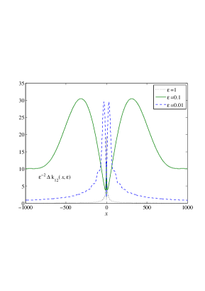
The above two characteristic values of the constant c210superscriptsubscript𝑐210c_{21}^{0} will be used in our numerical description of the behaviour of the remainder Δ​K1,Ρ​(x)Ξ”subscript𝐾1πœ€π‘₯\Delta K_{1,\varepsilon}(x) of the first order approximate factorization of the matrix (40).

In this example we have restricted our calculation to only the first step of the approximation. In principle, the procedure for the next steps has been already been described. However, there is no guarantee that the next step will be successful and a higher order guided perturbation will have been derived.

3.5 Example of a matrix which does not satisfy the solvability conditions

Simple changes to the matrix GΡ​(x)subscriptπΊπœ€π‘₯{G}_{\varepsilon}(x) can lead to a violation of the solvability conditions for the corresponding boundary value problem. Let us consider

G^Ρ​(x)=(x2+x​i​(βˆ’18+8​ei​Ρ​x+8​eβˆ’i​Ρ​x)βˆ’1x2+1x​i​(24βˆ’16​ei​Ρ​xβˆ’8​eβˆ’i​Ρ​x)x2+1x​i​(βˆ’12+4​ei​Ρ​x+8​eβˆ’i​Ρ​x)x2+1x2+x​i​(18βˆ’8​ei​Ρ​xβˆ’8​eβˆ’i​Ρ​x)βˆ’1x2+1).subscript^πΊπœ€π‘₯superscriptπ‘₯2π‘₯𝑖188superscriptπ‘’π‘–πœ€π‘₯8superscriptπ‘’π‘–πœ€π‘₯1superscriptπ‘₯21π‘₯𝑖2416superscriptπ‘’π‘–πœ€π‘₯8superscriptπ‘’π‘–πœ€π‘₯superscriptπ‘₯21missing-subexpressionmissing-subexpressionπ‘₯𝑖124superscriptπ‘’π‘–πœ€π‘₯8superscriptπ‘’π‘–πœ€π‘₯superscriptπ‘₯21superscriptπ‘₯2π‘₯𝑖188superscriptπ‘’π‘–πœ€π‘₯8superscriptπ‘’π‘–πœ€π‘₯1superscriptπ‘₯21\hat{G}_{\varepsilon}(x)=\left(\begin{array}[]{cc}\frac{x^{2}+xi(-18+8e^{i\varepsilon x}+8e^{-i\varepsilon x})-1}{x^{2}+1}&\frac{xi(24-16e^{i\varepsilon x}-8e^{-i\varepsilon x})}{x^{2}+1}\\ &\\ \frac{xi(-12+4e^{i\varepsilon x}+8e^{-i\varepsilon x})}{x^{2}+1}&\frac{x^{2}+xi(18-8e^{i\varepsilon x}-8e^{-i\varepsilon x})-1}{x^{2}+1}\end{array}\right). (58)

As before, G^0​(x)=G0​(x)subscript^𝐺0π‘₯subscript𝐺0π‘₯\hat{G}_{0}(x)={G}_{0}(x), and thus G^0​(x)subscript^𝐺0π‘₯\hat{G}_{0}(x) possesses a factorization with partial indices Ο°1=1,Ο°2=βˆ’1formulae-sequencesubscriptitalic-Ο°11subscriptitalic-Ο°21{\varkappa}_{1}=1,{\varkappa}_{2}=-1.

We note that

G^Ρ​(x)=GΡ​(x)+(0βˆ’x​i​(4​ei​Ρ​xβˆ’4​eβˆ’i​Ρ​x)x2+100).subscript^πΊπœ€π‘₯subscriptπΊπœ€π‘₯0π‘₯𝑖4superscriptπ‘’π‘–πœ€π‘₯4superscriptπ‘’π‘–πœ€π‘₯superscriptπ‘₯2100\hat{G}_{\varepsilon}(x)={G}_{\varepsilon}(x)+\left(\begin{array}[]{cc}0&-\frac{xi(4e^{i\varepsilon x}-4e^{-i\varepsilon x})}{x^{2}+1}\\ 0&0\end{array}\right).

We apply the above described asymptotic procedure to our matrix G^Ρ​(x)subscript^πΊπœ€π‘₯\hat{G}_{\varepsilon}(x), and show that this matrix cannot possess a bounded first order asymptotic factorization with the same partial indices as G^0​(x)subscript^𝐺0π‘₯\hat{G}_{0}(x).

The corresponding matrix is given by

N^Ρ​(x):=G^Ρ​(x)βˆ’Ξ›β€‹(x)=(x​i​(βˆ’16+8​ei​Ρ​x+8​eβˆ’i​Ρ​x)x2+1x​i​(24βˆ’16​ei​Ρ​xβˆ’8​eβˆ’i​Ρ​x)x2+1x​i​(βˆ’12+4​ei​Ρ​x+8​eβˆ’i​Ρ​x)x2+1x​i​(16βˆ’8​ei​Ρ​xβˆ’8​eβˆ’i​Ρ​x)x2+1)=assignsubscript^π‘πœ€π‘₯subscript^πΊπœ€π‘₯Ξ›π‘₯π‘₯𝑖168superscriptπ‘’π‘–πœ€π‘₯8superscriptπ‘’π‘–πœ€π‘₯superscriptπ‘₯21π‘₯𝑖2416superscriptπ‘’π‘–πœ€π‘₯8superscriptπ‘’π‘–πœ€π‘₯superscriptπ‘₯21π‘₯𝑖124superscriptπ‘’π‘–πœ€π‘₯8superscriptπ‘’π‘–πœ€π‘₯superscriptπ‘₯21π‘₯𝑖168superscriptπ‘’π‘–πœ€π‘₯8superscriptπ‘’π‘–πœ€π‘₯superscriptπ‘₯21absent\hat{N}_{\varepsilon}(x):=\hat{G}_{\varepsilon}(x)-\Lambda(x)=\left(\begin{array}[]{cc}\frac{xi(-16+8e^{i\varepsilon x}+8e^{-i\varepsilon x})}{x^{2}+1}&\frac{xi(24-16e^{i\varepsilon x}-8e^{-i\varepsilon x})}{x^{2}+1}\\ \frac{xi(-12+4e^{i\varepsilon x}+8e^{-i\varepsilon x})}{x^{2}+1}&\frac{xi(16-8e^{i\varepsilon x}-8e^{-i\varepsilon x})}{x^{2}+1}\end{array}\right)= (59)
=x​sin⁑Ρ​x2x2+1​(βˆ’32​i​sin⁑Ρ​x22​i​(24​sin⁑Ρ​x2+i​cos⁑Ρ​x2)βˆ’24​i​(sin⁑Ρ​x2βˆ’i​cos⁑Ρ​x2)32​i​sin⁑Ρ​x2).absentπ‘₯πœ€π‘₯2superscriptπ‘₯2132π‘–πœ€π‘₯22𝑖24πœ€π‘₯2π‘–πœ€π‘₯2missing-subexpressionmissing-subexpression24π‘–πœ€π‘₯2π‘–πœ€π‘₯232π‘–πœ€π‘₯2=\frac{x\sin\frac{\varepsilon x}{2}}{x^{2}+1}\left(\begin{array}[]{cc}-32i\sin\frac{\varepsilon x}{2}&2i(24\sin\frac{\varepsilon x}{2}+i\cos\frac{\varepsilon x}{2})\\ &\\ -24i(\sin\frac{\varepsilon x}{2}-i\cos\frac{\varepsilon x}{2})&32i\sin\frac{\varepsilon x}{2}\end{array}\right).

The first step of the asymptotic factorization leads to the problem

Ξ›+​(x)​N^1,Ξ΅+​(x)+N^1,Ξ΅βˆ’β€‹(x)β€‹Ξ›βˆ’β€‹(x)=M^0,Ρ​(x),superscriptΞ›π‘₯superscriptsubscript^𝑁1πœ€π‘₯superscriptsubscript^𝑁1πœ€π‘₯superscriptΞ›π‘₯subscript^𝑀0πœ€π‘₯\Lambda^{+}(x){{\hat{N}}}_{1,\varepsilon}^{+}(x)+{{\hat{N}}}_{1,\varepsilon}^{-}(x)\Lambda^{-}(x)=\hat{M}_{0,\varepsilon}(x), (60)

where the matrix function M^0,Ρ​(x)=N^Ρ​(x)subscript^𝑀0πœ€π‘₯subscript^π‘πœ€π‘₯\hat{M}_{0,\varepsilon}(x)=\hat{N}_{\varepsilon}(x) can be represented in the following form:

M^0,Ρ​(x)=M^0,Ξ΅+​(x)+M^0,Ξ΅βˆ’β€‹(x),subscript^𝑀0πœ€π‘₯superscriptsubscript^𝑀0πœ€π‘₯superscriptsubscript^𝑀0πœ€π‘₯\hat{M}_{0,\varepsilon}(x)=\hat{M}_{0,\varepsilon}^{+}(x)+\hat{M}_{0,\varepsilon}^{-}(x), (61)

and

M^0,Ξ΅+​(x)=(βˆ’8​i​(1βˆ’eβˆ’Ξ΅)x+i+8​x​i​(ei​Ρ​xβˆ’eβˆ’Ξ΅)x2+112​i​(1βˆ’eβˆ’Ξ΅)x+i+βˆ’16​x​i​(ei​Ρ​xβˆ’eβˆ’Ξ΅)x2+1βˆ’6​i​(1βˆ’eβˆ’Ξ΅)x+i+4​x​i​(ei​Ρ​xβˆ’eβˆ’Ξ΅)x2+18​i​(1βˆ’eβˆ’Ξ΅)x+i+βˆ’8​x​i​(ei​Ρ​xβˆ’eβˆ’Ξ΅)x2+1),superscriptsubscript^𝑀0πœ€π‘₯8𝑖1superscriptπ‘’πœ€π‘₯𝑖8π‘₯𝑖superscriptπ‘’π‘–πœ€π‘₯superscriptπ‘’πœ€superscriptπ‘₯2112𝑖1superscriptπ‘’πœ€π‘₯𝑖16π‘₯𝑖superscriptπ‘’π‘–πœ€π‘₯superscriptπ‘’πœ€superscriptπ‘₯216𝑖1superscriptπ‘’πœ€π‘₯𝑖4π‘₯𝑖superscriptπ‘’π‘–πœ€π‘₯superscriptπ‘’πœ€superscriptπ‘₯218𝑖1superscriptπ‘’πœ€π‘₯𝑖8π‘₯𝑖superscriptπ‘’π‘–πœ€π‘₯superscriptπ‘’πœ€superscriptπ‘₯21\hat{M}_{0,\varepsilon}^{+}(x)=\left(\begin{array}[]{cc}\frac{-8i(1-e^{-\varepsilon})}{x+i}+\frac{8xi(e^{i\varepsilon x}-e^{-\varepsilon})}{x^{2}+1}&\frac{12i(1-e^{-\varepsilon})}{x+i}+\frac{-16xi(e^{i\varepsilon x}-e^{-\varepsilon})}{x^{2}+1}\\ \frac{-6i(1-e^{-\varepsilon})}{x+i}+\frac{4xi(e^{i\varepsilon x}-e^{-\varepsilon})}{x^{2}+1}&\frac{8i(1-e^{-\varepsilon})}{x+i}+\frac{-8xi(e^{i\varepsilon x}-e^{-\varepsilon})}{x^{2}+1}\end{array}\right), (62)
M^0,Ξ΅βˆ’β€‹(x)=(βˆ’8​i​(1βˆ’eβˆ’Ξ΅)x+i+8​x​i​(eβˆ’i​Ρ​xβˆ’eβˆ’Ξ΅)x2+112​i​(1βˆ’eβˆ’Ξ΅)x+i+βˆ’8​x​i​(eβˆ’i​Ρ​xβˆ’eβˆ’Ξ΅)x2+1βˆ’6​i​(1βˆ’eβˆ’Ξ΅)x+i+8​x​i​(eβˆ’i​Ρ​xβˆ’eβˆ’Ξ΅)x2+18​i​(1βˆ’eβˆ’Ξ΅)x+i+βˆ’8​x​i​(eβˆ’i​Ρ​xβˆ’eβˆ’Ξ΅)x2+1).superscriptsubscript^𝑀0πœ€π‘₯8𝑖1superscriptπ‘’πœ€π‘₯𝑖8π‘₯𝑖superscriptπ‘’π‘–πœ€π‘₯superscriptπ‘’πœ€superscriptπ‘₯2112𝑖1superscriptπ‘’πœ€π‘₯𝑖8π‘₯𝑖superscriptπ‘’π‘–πœ€π‘₯superscriptπ‘’πœ€superscriptπ‘₯216𝑖1superscriptπ‘’πœ€π‘₯𝑖8π‘₯𝑖superscriptπ‘’π‘–πœ€π‘₯superscriptπ‘’πœ€superscriptπ‘₯218𝑖1superscriptπ‘’πœ€π‘₯𝑖8π‘₯𝑖superscriptπ‘’π‘–πœ€π‘₯superscriptπ‘’πœ€superscriptπ‘₯21\hat{M}_{0,\varepsilon}^{-}(x)=\left(\begin{array}[]{cc}\frac{-8i(1-e^{-\varepsilon})}{x+i}+\frac{8xi(e^{-i\varepsilon x}-e^{-\varepsilon})}{x^{2}+1}&\frac{12i(1-e^{-\varepsilon})}{x+i}+\frac{-8xi(e^{-i\varepsilon x}-e^{-\varepsilon})}{x^{2}+1}\\ \frac{-6i(1-e^{-\varepsilon})}{x+i}+\frac{8xi(e^{-i\varepsilon x}-e^{-\varepsilon})}{x^{2}+1}&\frac{8i(1-e^{-\varepsilon})}{x+i}+\frac{-8xi(e^{-i\varepsilon x}-e^{-\varepsilon})}{x^{2}+1}\end{array}\right). (63)

Bounded solutions to (60) have to satisfy the relation

N^1,Ξ΅+​(x)=(Ξ›+​(x))βˆ’1​[M^0,Ξ΅+​(x)βˆ’C^0],N^1,Ξ΅βˆ’β€‹(x)=[M^0,Ξ΅βˆ’β€‹(x)+C^0]​(Ξ›βˆ’β€‹(x))βˆ’1,formulae-sequencesuperscriptsubscript^𝑁1πœ€π‘₯superscriptsuperscriptΞ›π‘₯1delimited-[]superscriptsubscript^𝑀0πœ€π‘₯subscript^𝐢0superscriptsubscript^𝑁1πœ€π‘₯delimited-[]superscriptsubscript^𝑀0πœ€π‘₯subscript^𝐢0superscriptsuperscriptΞ›π‘₯1{{\hat{N}}}_{1,\varepsilon}^{+}(x)=(\Lambda^{+}(x))^{-1}\left[\hat{M}_{0,\varepsilon}^{+}(x)-\hat{C}_{0}\right],\;{{\hat{N}}}_{1,\varepsilon}^{-}(x)=\left[\hat{M}_{0,\varepsilon}^{-}(x)+\hat{C}_{0}\right](\Lambda^{-}(x))^{-1}, (64)

where C^0=(c^i​j0)subscript^𝐢0subscript^𝑐𝑖superscript𝑗0\hat{C}_{0}=(\hat{c}_{i}j^{0}) is a constant matrix.

In this case

m^0,12+​(i)=6​(1βˆ’eβˆ’Ξ΅)βˆ’8​Ρ​eβˆ’Ξ΅,m^0,12βˆ’β€‹(βˆ’i)=βˆ’6​(1βˆ’eβˆ’Ξ΅)+4​Ρ​eβˆ’Ξ΅,formulae-sequencesuperscriptsubscript^π‘š012𝑖61superscriptπ‘’πœ€8πœ€superscriptπ‘’πœ€superscriptsubscript^π‘š012𝑖61superscriptπ‘’πœ€4πœ€superscriptπ‘’πœ€\hat{m}_{0,12}^{+}(i)=6(1-e^{-\varepsilon})-8\varepsilon e^{-\varepsilon},\quad\hat{m}_{0,12}^{-}(-i)=-6(1-e^{-\varepsilon})+4\varepsilon e^{-\varepsilon},

and thus, the solvability condition m^0,12+​(i)=βˆ’m^0,12βˆ’β€‹(βˆ’i)superscriptsubscript^π‘š012𝑖superscriptsubscript^π‘š012𝑖\hat{m}_{0,12}^{+}(i)=-\hat{m}_{0,12}^{-}(-i) is satisfied only for Ξ΅=0πœ€0\varepsilon=0. For all Ξ΅β‰ 0πœ€0\varepsilon\not=0, there is no approximate solution (up to Ξ΅2superscriptπœ€2\varepsilon^{2}) of the functional equation (similarly to (45)).

Remark 3.8

Note that, by construction,

G^Ρ​(x)βˆ’GΡ​(x)=(0O​(Ξ΅)00),Ξ΅β†’0.formulae-sequencesubscript^πΊπœ€π‘₯subscriptπΊπœ€π‘₯0π‘‚πœ€00β†’πœ€0\hat{G}_{\varepsilon}(x)-G_{\varepsilon}(x)=\left(\begin{array}[]{cc}0&O(\varepsilon)\\ 0&0\end{array}\right),\;\varepsilon\to 0.

Hence, G^Ρ​(x)subscript^πΊπœ€π‘₯\hat{G}_{\varepsilon}(x) presents an example of the regular perturbation of G^0​(x)subscript^𝐺0π‘₯\hat{G}_{0}(x), for which no regular k-guided perturbation (k>1π‘˜1k>1) exists while construction of a singular perturbation remains an open problem.

4 Numerical examples and discussion

In this section, we analyse the quality of the approximation provided by the 2-guided perturbation performed in Section  3 3.4.

First, we consider the case when c21=0subscript𝑐210c_{21}=0, and thus the limiting value of the remainder, Δ​K1​ΡΔsubscript𝐾1πœ€\Delta K_{1\varepsilon} does not vanish at infinity. Specifically, we estimate the element on the main diagonal in the following way:

Δ​kj​j​(∞)=16​(1βˆ’eβˆ’Ξ΅+Ρ​eβˆ’Ξ΅)=64​Ρ2βˆ’96​Ρ3+O​(Ξ΅4),Ξ΅β†’0,j=1,2.formulae-sequenceΞ”subscriptπ‘˜π‘—π‘—161superscriptπ‘’πœ€πœ€superscriptπ‘’πœ€64superscriptπœ€296superscriptπœ€3𝑂superscriptπœ€4formulae-sequenceβ†’πœ€0𝑗12\Delta k_{jj}(\infty)=16\left(1-e^{-\varepsilon}+\varepsilon e^{-\varepsilon}\right)=64\varepsilon^{2}-96\varepsilon^{3}+O(\varepsilon^{4}),\quad\varepsilon\to 0,\quad j=1,2.

In Fig. 2 a) and b), those components are presented in their normalised forms. We can see that the estimate is true (see the discussion on the small parameter following formula (56)). Furthermore, the matrix converges to its limiting values more quickly for larger values of the small parameter, while the oscillations decay more slowly for smaller values.
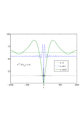
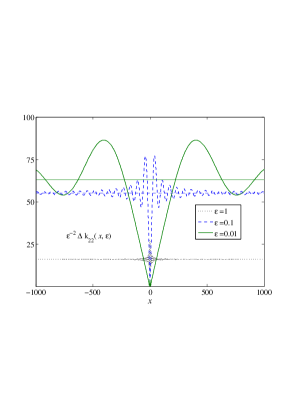
Refer to caption
Refer to caption
Figure 2: Diagonal elements, Δ​kj​j​(x,Ξ΅)Ξ”subscriptπ‘˜π‘—π‘—π‘₯πœ€\Delta k_{jj}(x,\varepsilon), j=1,2𝑗12j=1,2, of matrix Δ​K1,Ρ​(x)Ξ”subscript𝐾1πœ€π‘₯\Delta K_{1,\varepsilon}(x) defined in for various values of parameter Ξ΅πœ€\varepsilon, the constant c210=0superscriptsubscript𝑐2100c_{21}^{0}=0. The elements are normalised to the value of parameter Ξ΅2superscriptπœ€2\varepsilon^{2}.

In Fig. 3 a) and b), the remaining two components are depicted in the same normalised forms. Preserving the same estimate, where Δ​K1,Ρ​(x)=O​(Ξ΅2)Ξ”subscript𝐾1πœ€π‘₯𝑂superscriptπœ€2\Delta K_{1,\varepsilon}(x)=O(\varepsilon^{2}) as Ξ΅β†’0β†’πœ€0\varepsilon\to 0, the components now decay to O​(xβˆ’1)𝑂superscriptπ‘₯1O(x^{-1}), as |x|β†’βˆžβ†’π‘₯|x|\to\infty. The trend is also clearly visible here, that the smaller Ξ΅πœ€\varepsilon is, the slower it converges to its limiting value. In other words, the small parameter Ξ΅πœ€\varepsilon determines the magnitude of the reminder matrix, but the oscillations are larger in this case, and more pronounced along the real axis.
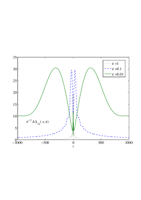
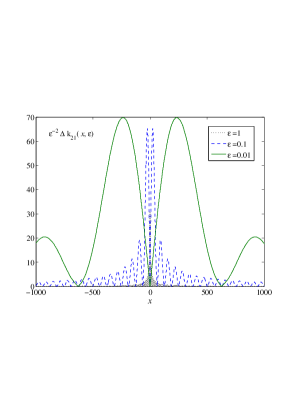
Refer to caption
Refer to caption
Figure 3: The other two elements, Δ​ki​j​(x,Ξ΅)Ξ”subscriptπ‘˜π‘–π‘—π‘₯πœ€\Delta k_{ij}(x,\varepsilon), i+j=3𝑖𝑗3i+j=3, of matrix Δ​K1,Ρ​(x)Ξ”subscript𝐾1πœ€π‘₯\Delta K_{1,\varepsilon}(x) for Ξ΅=1;0.1;0.01πœ€10.10.01\varepsilon=1;0.1;0.01, and constant c210=0superscriptsubscript𝑐2100c_{21}^{0}=0. It is clear that both entries vanish at infinity ki​jβ†’0β†’subscriptπ‘˜π‘–π‘—0k_{ij}\to 0 as |x|β†’βˆžβ†’π‘₯|x|\to\infty.

Interestingly, the components on the main diagonal are comparable in value, but not equal, while the remaining two differ in value by almost a factor of two. Moreover, the latter are also two times smaller in magnitude then the diagonal elements.

The situation changes when we consider the second case, where c210=βˆ’8/3​(1βˆ’eβˆ’Ξ΅+Ρ​eβˆ’Ξ΅)superscriptsubscript𝑐210831superscriptπ‘’πœ€πœ€superscriptπ‘’πœ€c_{21}^{0}=-8/3(1-e^{-\varepsilon}+\varepsilon e^{-\varepsilon}). The respective graphs are presented in Fig. 4, 5. Now, all the components decay at infinity as O​(xβˆ’1)𝑂superscriptπ‘₯1O(x^{-1}), as |x|β†’βˆžβ†’π‘₯|x|\to\infty, and simultaneously have the same estimate of (O​(Ξ΅2)𝑂superscriptπœ€2O(\varepsilon^{2})) when Ξ΅β†’0β†’πœ€0\varepsilon\to 0, as predicted. The magnitudes of the components are, however, more balanced in the sup norm ‖Δ​K1,Ξ΅(1)β€–>2​‖Δ​K1,Ξ΅(2)β€–normΞ”superscriptsubscript𝐾1πœ€12normΞ”superscriptsubscript𝐾1πœ€2\|\Delta K_{1,\varepsilon}^{(1)}\|>2\|\Delta K_{1,\varepsilon}^{(2)}\|. This demonstrates that we can choose an optimal approximation preserving some specified requirement by varying the value of the arbitrary constant c21subscript𝑐21c_{21}. Comparing these two cases, it is clear that the second is preferable to the first for the reasons discussed above.
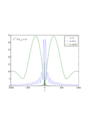
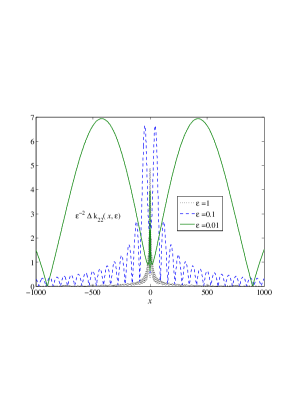
Refer to caption
Refer to caption
Figure 4: Diagonal elements, Δ​kj​j​(x,Ξ΅)Ξ”subscriptπ‘˜π‘—π‘—π‘₯πœ€\Delta k_{jj}(x,\varepsilon), j=1,2𝑗12j=1,2, of matrix Δ​K1,ΡΔsubscript𝐾1πœ€\Delta K_{1,\varepsilon}, for various Ξ΅πœ€\varepsilon, and the constant c210=βˆ’8/3​(1βˆ’eβˆ’Ξ΅+Ρ​eβˆ’Ξ΅)superscriptsubscript𝑐210831superscriptπ‘’πœ€πœ€superscriptπ‘’πœ€c_{21}^{0}=-8/3(1-e^{-\varepsilon}+\varepsilon e^{-\varepsilon}). The elements are normalised to the value of parameter Ξ΅2superscriptπœ€2\varepsilon^{2}. The horizontal lines show the limiting values of the normalised components at infinity.
Refer to caption
Refer to caption
Figure 5: The other two elements, Δ​ki​j​(x,Ξ΅)Ξ”subscriptπ‘˜π‘–π‘—π‘₯πœ€\Delta k_{ij}(x,\varepsilon), i+j=3𝑖𝑗3i+j=3, of matrix Δ​K1,Ρ​(x)Ξ”subscript𝐾1πœ€π‘₯\Delta K_{1,\varepsilon}(x) for Ξ΅=1;0.1;0.01πœ€10.10.01\varepsilon=1;0.1;0.01, and the constant c210=βˆ’8/3​(1βˆ’eβˆ’Ξ΅+Ρ​eβˆ’Ξ΅)superscriptsubscript𝑐210831superscriptπ‘’πœ€πœ€superscriptπ‘’πœ€c_{21}^{0}=-8/3(1-e^{-\varepsilon}+\varepsilon e^{-\varepsilon}). It is clear that both entries vanish at infinity ki​jβ†’0β†’subscriptπ‘˜π‘–π‘—0k_{ij}\to 0 as |x|β†’βˆžβ†’π‘₯|x|\to\infty.

Any specific factorization will of course require its own analyses. However, if the estimate

GΡ​(x)=o​(1),|x|β†’βˆž,formulae-sequencesubscriptπΊπœ€π‘₯π‘œ1β†’π‘₯G_{\varepsilon}(x)=o(1),\quad|x|\to\infty,

is true, then the reminder can be estimated by

Δ​K1,Ρ​(x)=(c110c120c210c220)2+o​(1),|x|β†’βˆž.formulae-sequenceΞ”subscript𝐾1πœ€π‘₯superscriptsuperscriptsubscript𝑐110superscriptsubscript𝑐120superscriptsubscript𝑐210superscriptsubscript𝑐2202π‘œ1β†’π‘₯\Delta K_{1,\varepsilon}(x)=\left(\begin{array}[]{cc}c_{11}^{0}&c_{12}^{0}\\ c_{21}^{0}&c_{22}^{0}\end{array}\right)^{2}+o(1),\quad|x|\to\infty.

We note that this property may change in the next step if we wish to and can continue the approximation procedure, (the conditions will remain valid for the next step). Here, the limiting values for the first step will also play their role. We can deliver a similar formula based on the two consequent approximations, where two sets of constants will then be involved: cj​lsubscript𝑐𝑗𝑙c_{jl} (first step) and dj​lsubscript𝑑𝑗𝑙d_{jl} (second step), j,l=1,2formulae-sequence𝑗𝑙12j,l=1,2.

Judging by the magnitude of the reminder for both the presented examples, we can conclude that the 2-guided perturbation may be sufficient for practical purposes. Thus, if even one approximation step is practically possible, meaning that the conditions (27)-(31) are satisfied, then we can use this approximation directly in solving the Wiener-Hopf equation.

To close, we must highlight that, if conditions (27)-(31) for matrix GΞ΅subscriptπΊπœ€G_{\varepsilon}, with unstable partial indices, are not satisfied, the question of how to compute a valuable approximate factorization for such a matrix-function remains open.

Acknoledgements The work is supported by the People Programme (Marie Curie Actions) of the European Union’s Seventh Framework Programme FP7/2007- 2013/ under REA grant agreement PIRSES-GA-2013-610547 - TAMER. GM acknowledges support from a Royal Society Wolfson Research Merit Award.

References

  • [1] Abrahams ID. 2000. Application of Pade approximants to Wiener-Hopf factorization, IMA Journal of Applied Mathematics, 65 (3).
  • [2] Abrahams ID, Davis AMJ and Smith SGL. 2008. Matrix Wiener-Hopf approximation for a partially clamped plate. Quarterly Journal of Mechanics and Applied Mathematics, 61 (2).
  • [3] Abrahams ID, and Lawrie JB. 1995. On the factorization of a class of Wiener-Hopf kernels. IMA Journal of Applied Mathematics, 55 (1).
  • [4] Bojarsky B. 1958. On stability of the Hilbert problem for holomorphic vector. Soobstch. AN GruzSSR 21 (4) (Russian).
  • [5] Crighton DG. 2001. Asymptotitc factorization of Wiener-Hopf kernels. Wave Motion 33 (1).
  • [6] Gakhov FD. 1977. Boundary Value Problems. Moscow, Nauka (3rd ed.) (Russian).
  • [7] Gohberg I, Kaashoek M, Spitkovski I. 2003. An overview of matrix factorization theory and operator applications. In Oper. Theory Adv. Appl. 141. Basel, BirkhΓ€user.
  • [8] Gohberg IT, Krein MG. 1958. Systems of integral equations on a half-line with kernels depending on the difference of arguments. Uspekhi mat. nauk XIII (2) (Russian).
  • [9] Gohberg IT, Krein MG. 1958. On stable system of partial indices of the Hilbert problem for several unknown functions. Doklady AN SSSR 119 (5) (Russian).
  • [10] Hurd RA. 1976. The Wiener-Hopf-Hilbert method for diffraction problems, Can. J. Phys., 54.
  • [11] Hurd RA, LΓΌneburg E. 1981. Scattering by hard and soft paralel half-planes, Can. J. Phys., 59.
  • [12] Kisil A. 2013. A constructive method for an approximate solution to scalar Wiener-Hopf equations, Proc. R. Soc. A, 469, 20120721.
  • [13] Kisil A. 2015. Stability analysis of matrix Wiener-Hopf factorization of Daniele-Khrapkov class and reliable approximate factorization, Proc. R. Soc. A, 471, 20150146.
  • [14] Lawrie JB, Abrahams ID. 2007. A brief historical perspective of the Wiener-Hopf technique. J. Eng. Math. 9 (4).
  • [15] Litvinchuk GS. 1967. Two theorems on the stability of the partial indices of Riemann’s boundary value problem and their applications. Izv. Vyssh. Uchebn. Zaved. Mat. (12) (Russian).
  • [16] Litvinchuk GS, Spitkovsky IM. 1987. Factorization of measurable matrix functions. Basel-Boston, BirkhΓ€user.
  • [17] Meister E, Speck F-O. 1989. Modern Wiener-Hopf methods in diffraction theory, In: In: Ordinary and partial differential equations, Vol. II, Pitman Res. Notes. Math. Ser., 216.
  • [18] Mishuris GS, Movchan NV, and Movchan AB. 2007. Dynamic mode-III interface crack in a bi-material strip. International Journal of Fracture 166.
  • [19] Mishuris G, Rogosin S. 2014. An asymptotic method of a class of matrix functions. Proc. R. Soc. A 470.
  • [20] Mishuris G, Rogosin S. 2016. Constructive methods for factorization of matrix-functions. IMA J. Appl. Math. 81 (2).
  • [21] Mishuris G, Rogosin S. 2016. Factorization of a class of matrix-functions with stable partial indices. Math. Meth. Appl. Sci. 39 (13).
  • [22] Muskhelishvili NI. 1968. Singular Integral Equations. Moscow, Nauka (3rd ed.) (Russian).
  • [23] Noble B. 1988. Methods based on the Wiener-Hopf Technique. New York, Chelsea Publishing Company.
  • [24] Piccolroaz A, Mishuris G, Movchan A. 2007. Evaluation of the Lazarus-Leblond constants in the asymptotic model of the interfacial wavy crack. Journal of the Mechanics and Physics of Solids, 55.
  • [25] Piccolroaz A, Mishuris G, Movchan A. 2009. Symmetric and skew-symmetric weight functions in 2D perturbation models for semi-infinite interfacial cracks. Journal of the Mechanics and Physics of Solids, 57.
  • [26] Piccolroaz A, Mishuris G, Movchan A, Movchan N. 2012. Perturbation analysis of Mode III interfacial cracks advancing in a dilute heterogeneous material. International Journal of Solids and Structures, 49.
  • [27] Vekua NP. 1967. Systems of singular integral equations. Groningen, P. Noordhoff.