Internal and external potential-field estimation from regional vector data at varying satellite altitude

Abstract

When modeling global satellite data to recover a planetary magnetic or gravitational potential field and evaluate it elsewhere, the method of choice remains their analysis in terms of spherical harmonics. When only regional data are available, or when data quality varies strongly with geographic location, the inversion problem becomes severely ill-posed. In those cases, adopting explicitly local methods is to be preferred over adapting global ones (e.g., by regularization). Here, we develop the theory behind a procedure to invert for planetary potential fields from vector observations collected within a spatially bounded region at varying satellite altitude. Our method relies on the construction of spatiospectrally localized bases of functions that mitigate the noise amplification caused by downward continuation (from the satellite altitude to the planetary surface) while balancing the conflicting demands for spatial concentration and spectral limitation. The ‘altitude-cognizant’ gradient vector Slepian functions (AC-GVSF) were first employed in a preceding paper. They enjoy a noise tolerance under downward continuation that is much improved relative to the ‘classical’ gradient vector Slepian functions (CL-GVSF), which do not factor satellite altitude into their construction. Furthermore, venturing beyond the realm of their first application, in the present article we extend the theory to being able to handle both internal and external potential-field estimation. Solving simultaneously for internal and external fields in the same setting of regional data availability reduces internal-field artifacts introduced by downward-continuing unmodeled external fields, as we show with numerical examples. We explain our solution strategies on the basis of analytic expressions for the behavior of the estimation bias and variance of models for which signal and noise are uncorrelated, (essentially) space- and bandlimited, and spectrally (almost) white. The AC-GVSF are optimal linear combinations of vector spherical harmonics. Their construction is not altogether very computationally demanding when the concentration domains (the regions of spatial concentration) have circular symmetry, e.g., on spherical caps or rings — even when the spherical-harmonic bandwidth is large. Data inversion proceeds by solving for the expansion coefficients of truncated function sequences, by least-squares analysis in a reduced-dimensional space. Hence, our method brings high-resolution regional potential-field modeling from incomplete and noisy vector-valued satellite data within reach of contemporary desktop machines.

1 Introduction

Potential fields such as gravity and magnetic fields provide indispensable information about planetary or lunar structure and evolution Kaula (1968); Lambeck (1988); Langel and Hinze (1998); Merrill et al. (1998). At the scale of the globe for Earth and Moon, and more generally for other planets and their moons, the vast majority of the data is derived from satellite missions Connerney (2015); Wieczorek (2015). Recording gravity and magnetic fields in space is an engineering problem of instrumentation. Mapping such fields from space, back onto the planetary surface where they originate, and separately from any fields generated externally, down to the body of interest, is a problem of inversion Plattner and Simons (2015b); Sabaka et al. (2015). Regional modeling is predicated on the ability to include data collected at varying satellite altitude, alleviating noise amplification under ‘downward continuation’, and, in particular in the case of magnetic field modeling, taking external fields into account. The full estimation problem as we consider it here consists in determining ‘best’ models — suitable for evaluation at the surface of the planetary body, and geological interpretation as far as accuracy and resolution permit — of an internally generated field noisily observed at a scattered, areally-limited set of locations taken at varying satellite altitude, in the presence of an external field.

Beginning with Gauss (1839), the parameterization of the solution in terms of global basis functions, spherical Backus et al. (1996) or ellipsoidal Bölling and Grafarend (2005) harmonics, remains today a popular practical approach Sneeuw (1994). At the other end of the modeling spectrum are local methods, specifically, those based on gridded sets of monopoles (e.g. O’Brien and Parker, 1994), equivalent-source dipoles (e.g. Langel and Hinze, 1998), or point masses (e.g. Baur and Sneeuw, 2011). In-between those extremes of spectral and spatial selectivity (for a classification, see Freeden and Michel, 1999; Freeden et al., 2016) lies a variety of methods that uses functions such as radial basis functions (e.g. Schmidt et al., 2007), mascons (e.g. Watkins et al., 2015) and spherical cap harmonics (e.g. Thébault et al., 2006; Langlais et al., 2010), spherical-harmonic splines (e.g. Shure et al., 1982; Amirbekyan et al., 2008) and wavelets Holschneider et al. (2003); Mayer and Maier (2006); Gerhards (2012). Among the constructively ‘spatio-spectrally localized’ spherical functions (e.g. Lesur, 2006) features the general class of ‘Slepian functions’ Simons et al. (2006); Plattner and Simons (2014); Simons and Plattner (2015) upon which we build our present work.

Building new bases (or ‘frames’, in a wider sense) by the judiciously weighted linear combination of spherical harmonics, which most of the above localization methods have in common, provides a natural way to respect the harmonicity of the potential fields under study. When the spherical-harmonic expansion coefficients of a potential field at a certain altitude are ‘known’, downward continuation to the zero height of the planetary surface, usually approximated by a sphere, amounts to a simple reevaluation via multiplication of the coefficients with factors that depend on the radii of the measurement sphere and the planet (e.g. Blakely, 1995; Backus et al., 1996; Dahlen and Tromp, 1998). In the case of imperfect knowledge, however, numerical and statistical stability limit the spatial resolution of the reevaluated fields that can be obtained in this way, depending on the relative altitude and the signal-to-noise ratios of the coefficients. Such difficulties are exacerbated if the source of the uncertainty, fundamentally, lies in the original data being available over an incomplete portion of the measurement sphere Kaula (1967); Xu (1992); Trampert and Snieder (1996); Simons and Dahlen (2006); Schachtschneider et al. (2012). For such problems, inversion methods that rely on spherical-harmonics based localized basis functions confer efficiency and stability, dimensional reduction, and the overall ease and ability to produce and downward-continue regional potential-field models with less statistical a priori information or numerical regularization.

Satellite data coverage is far from being always ‘global’. Coverage may be only regional, as is the case over Mercury Solomon et al. (2001, 2007), or data quality may vary due to spatial variations of signal-to-noise levels or satellite altitude, rendering a geographical restriction of the area of interest desirable. Such was the situation for Mars Albee et al. (2001), where Plattner and Simons (2015a) selected low-altitude nighttime magnetic-field data for inversion using the ‘altitude-cognizant gradient vector Slepian functions’ that are the subject of this paper, resulting in a new lithospheric magnetic-field model of the Martian South Pole. They subtracted an external-field model made independently by Olsen et al. (2010a) from the data prior to inversion. In the present paper, we treat the estimation of internally and externally generated fields as an inverse problem that considers both jointly.

Our method traces its history to the one-dimensional theory of ‘prolate spheroidal wave functions’ by Slepian and Pollak (1961), its applications in signal processing Slepian (1983), and especially its extensions to scalar spherical fields by Simons et al. (2006) and Simons and Dahlen (2006), to spherical vector fields by Plattner and Simons (2014), and to gradient vector spherical functions (curl-free potential fields) by Plattner and Simons (2015b). In the above cited works, satellite altitude, though explicitly considered within the context of the inverse problem, was never a factor in the optimization construction of the Slepian functions, and so we will term them ‘canonical’ or ‘classical’. In particular, the functions of Plattner and Simons (2015b) will hereafter be known as ‘classical gradient vector Slepian functions’ (CL-GVSF). In contrast, the construction by Plattner and Simons (2015a), reformulated in the present paper, does incorporate satellite altitude directly, hence their designation ‘altitude-cognizant gradient vector Slepian functions’ (AC-GVSF). The CL-GVSF solve a spatial (surface) optimization problem for bandlimited functions, while the AC-GVSF incorporate optimization under downward-continuation from satellite altitude. Using the AC-GVSF for satellite-data inversion is different than using the CL-GVSF basis. In the latter case, vector-field measurements are first inverted for a best-fitting model at altitude, and the results are downward-continued afterwards. As Plattner and Simons (2015b) already noted in their Sections 7.1–7.2, in that case, the model at the planetary surface is potentially biased by power in the high spherical-harmonic degrees leaking in through the downward continuation. This bias is a consequence of using functions that solely optimize spatial concentration within a given region. The general method presented here aims at overcoming these issues.

We construct a basis of functions from linear combinations of gradient vector spherical harmonics by solving an optimization problem that incorporates the satellite altitude at which the data are acquired. We present two versions of an inversion method that use different forms of the altitude-cognizant gradient vector Slepian functions (AC-GVSF). In the first method we assume that external fields are not present, or have been removed from the data by prior analysis. In our second method, we model external fields simultaneously while solving for the internal field. Only the first approach was used by Plattner and Simons (2015a), and they did not present a complete mathematical analysis, as we do here. Notation and preliminary considerations can be found Section 2. A statement of the problem that we solve is found in Section 3. The body of the paper is arranged around the three questions ‘what?’, ‘how?’, and ‘why?’. Sections 4–8 cover the question ‘what’ and touch on the question ‘how?’. Sections 9 and 10 answer the question ‘why?’. Finally, the Appendix focuses again on the question ‘how?’, in more detail. More precisely, in Section 4 we present the purely internal-field AC-GVSF that we will use in Section 6 to solve for a potential-field model from purely internal-field regional vector data. Section 5 describes the construction of internal and external field AC-GVSF that we use, in Section 7, to solve simultaneously for the internal and external potential field from regional satellite data with varying altitude. We test both methods on a simulated data set in Section 8 and investigate the effect of neglecting to account for an external field. In Sections 9 and 10 we provide a more in-depth analysis of the relationship of our new Slepian functions to the generic vector spherical Slepian functions presented by Plattner and Simons (2014) and showcase their mathematical and statistical properties. We summarize our findings in Section 11 and explain methods to significantly decrease the computational costs of high spherical-harmonic degree calculations in the Appendix.

Compared to other regional methods, the AC-GVSF approach has the overall advantage that all calculations happen within a space spanned by bandlimited spherical-harmonics, the natural basis for source-free potential fields outside a sphere (Section 2.1). Our method can be interpreted as a computationally tractable approximation to the truncated singular-value decomposition of the full spherical-harmonic global problem focused on a chosen region. The AC-GVSF are easy to use, computationally efficient, and work with discrete data collected at varying satellite altitude. A benchmark comparison test with other methods would be beyond the scope of this article. Instead we summarize where we discern the main differences with other regional methods. The popular Revised Spherical Cap Harmonic Analysis (R-SCHA) method by Thébault et al. (2006) fits data using basis functions that solve Laplace’s equation inside a cone covering the chosen region with appropriate boundary conditions. Our method allows for the separation of internal- and external fields (with bias, as we show in eqs 146–149), which can not be readily achieved using R-SCHA Thébault et al. (2006). Potential fields obtained using AC-GVSF can be expressed in a wavelength-dependent power spectrum, which appears to not be possible for R-SCHA, at least for non-trivial boundary conditions Thébault et al. (2006). The spherical wavelet methods by Mayer and Maier (2006) and Gerhards (2011, 2012, 2014) provide another powerful regional approach. To the best of our knowledge these methods assume that the satellite orbit is of constant altitude, which is not required in our method. Discrete-source methods such as monopoles O’Brien and Parker (1994), equivalent dipoles Langel and Hinze (1998), or point-mass modeling Baur and Sneeuw (2011) require the assumption of a known source depth. In special cases this may be justified but in general, the choice of the source depth requires independent consideration. By solving for the uniquely constrained potential field on the planetary surface, instead of the non-uniquely constrained physical sources themselves, our method avoids this problem.

We assume that the magnetic field that we solve for is static, in that we do not incorporate a direct time dependence. To avoid temporal aliasing, the data should be binned into episodic clusters before inversion and then inverted individually using the same set of AC-GVSF.

2 Preliminary considerations

In this section we establish the mathematical building blocks and develop a consistent notation for the development in the rest of the paper.

2.1 Scalar spherical harmonics for potential fields

In a coordinate system originating at the planetary or lunar center we define a spherical shell $\circledcirc=\{\boldsymbol{r}\mid{r_{p}}\leq\lVert\boldsymbol{r}\rVert=r\leq{r_{q}}\}$ between an inner sphere with radius ${r_{p}}$, an approximation of the planetary surface, and an outer sphere defined by the radius ${r_{q}}$, outside of the satellite orbit ${r_{s}}$. Fig. 1 shows the relative location of the different radial positions considered as discussed in this section and beyond. Our goal is to ‘map’ a magnetic or gravity measurement made at an altitude $r-{r_{p}}$ above the planet, ${r_{p}}<r<{r_{q}}$, onto a potential evaluated on the sphere of radius ${r_{p}}$. In the absence of field sources within the spherical shell $\circledcirc$, the only sources lying either within the ball of radius ${r_{p}}$ or outside of the sphere of radius ${r_{q}}$, the true “full” field inside $\circledcirc$ is the superposition of two scalar potentials: an ‘internal’ field $V$, and an ‘external’ field $W$. Both fields are ‘harmonic’: they solve the spherical Laplace equation Blakely (1995); Snieder (2004); Newman (2016)

$$\nabla^{2}\left[V(r\boldsymbol{\hat{r}})+W(r\boldsymbol{\hat{r}})\right]=0,\qquad{r_{p}}<r,{r_{s}}<{r_{q}},$$ (1)

where the usual Laplacian $\nabla^{2}=\partial^{2}_{r}+2r^{-1}\partial_{r}+r^{-2}\nabla_{1}^{2}$, and surface Laplacian $\nabla_{1}^{2}=\partial_{\theta}^{2}+\cot{\theta}\,\partial_{\theta}+(\sin{\theta})^{-2}\partial_{\phi}^{2}$ for colatitude $0\leq\theta\leq\pi$ and longitude $0\leq\phi<2\pi$. For a point $\boldsymbol{\hat{r}}$ on the surface of the unit sphere $\Omega=\{\boldsymbol{\hat{r}}\mid\lVert\boldsymbol{\hat{r}}\rVert=1\}$, we define the orthonormal set of scalar spherical-harmonics as do Dahlen and Tromp (1998), Simons et al. (2006), and Plattner and Simons (2014, 2015a, 2015b). These are given by

$$Y_{lm}(\boldsymbol{\hat{r}})=Y_{lm}(\theta,\phi) =\begin{cases}\sqrt{2}X_{l\lvert m\rvert}(\theta)\cos m\phi&\text{if }-l\leq m<0,\\ X_{l0}(\theta)&\text{if }m=0,\\ \sqrt{2}X_{lm}(\theta)\sin m\phi&\text{if }0<m\leq l,\end{cases}$$ (2)

$$X_{lm}(\theta) =(-1)^{m}\left(\frac{2l+1}{4\pi}\right)^{1/2}\left[\frac{(l-m)!}{(l+m)!}\right]^{1/2}\frac{1}{2^{l}l!}(1-\mu^{2})^{m/2}\left(\frac{d}{d\mu}\right)^{l+m}(\mu^{2}-1)^{l},$$ (3)

where $0\leq l\leq\infty$ is the angular degree of the spherical harmonic, and $-l\leq m\leq l$ its angular order. As shown by Backus (1986) and Freeden and Schreiner (2009), among others, the general solution to eq. (1) involves linear combinations of the functions (2)–(3), the ‘inner’ solid harmonics $r^{l}Y_{lm}$, and the ‘outer’ solid harmonics, $r^{-l-1}Y_{lm}$. The outer harmonics extinguish at infinity and, therefore, are a suitable basis for the functions $V$, generated by internal sources. The inner harmonics vanish at the center of the coordinate system, and, therefore, form the basis for the functions $W$, generated by external sources. Inside the shell $\circledcirc$, the individual fields are represented as

$$V(r\boldsymbol{\hat{r}}) =\sum_{l=0}^{\infty}\sum_{m=-l}^{l}\left(\frac{r}{{r_{p}}}\right)^{-l-1}v^{r_{p}}_{lm}Y_{lm}(\boldsymbol{\hat{r}}),\quad\mbox{with}\quad v^{r_{p}}_{lm}=\int_{\Omega}V({r_{p}}\boldsymbol{\hat{r}})Y_{lm}(\boldsymbol{\hat{r}})\,d\Omega,$$ (4)

$$W(r\boldsymbol{\hat{r}}) =\sum_{l=1}^{\infty}\sum_{m=-l}^{l}\left(\frac{r}{{r_{q}}}\right)^{l}w^{r_{q}}_{lm}Y_{lm}(\boldsymbol{\hat{r}}),\quad\mbox{with}\quad w^{r_{q}}_{lm}=\int_{\Omega}W({r_{q}}\boldsymbol{\hat{r}})Y_{lm}(\boldsymbol{\hat{r}})\,d\Omega.$$ (5)

In eqs (4)–(5) we selected ${r_{p}}$ and ${r_{q}}$ as reference radii for the coefficients $v^{r_{p}}_{lm}$ and $w^{r_{q}}_{lm}$, respectively. We collect bandlimited subsets of the spherical-harmonic coefficients $v^{r_{p}}_{lm}$, for the internal field in a vector $\mathrm{v}_{L}^{r_{p}}$, and a set of $w^{r_{q}}_{lm}$ for the external field in a vector $\mathrm{w}_{L_{o}}^{r_{q}}$,

$$\mathrm{v}_{L}^{r_{p}}=\begin{pmatrix}v^{r_{p}}_{00}&\cdots&v^{r_{p}}_{lm}&\cdots&v^{r_{p}}_{LL}\end{pmatrix}^{T}\quad\mbox{and}\quad\mathrm{w}_{L_{o}}^{r_{q}}=\begin{pmatrix}w^{r_{q}}_{1\,-1}&\cdots&w^{r_{q}}_{lm}&\cdots&w^{r_{q}}_{{L_{o}}{L_{o}}}\end{pmatrix}^{T}.$$ (6)

We assemble the scalar spherical harmonics $Y_{lm}$ into an infinite-dimensional column vector $\mathcal{Y}$ that we think of as consisting of two parts,

$$\mathcal{Y}=\begin{pmatrix}\mathcal{Y}_{L}^{\mathcal{T}}\quad\mathcal{Y}_{>L}^{\mathcal{T}}\end{pmatrix}^{\mathcal{T}}=\begin{pmatrix}Y_{00}\quad\mathcal{Y}_{L_{o}}^{\mathcal{T}}\quad\mathcal{Y}_{>{L_{o}}}^{\mathcal{T}}\end{pmatrix}^{\mathcal{T}}.$$ (7)

As to the bandlimited, $(L+1)^{2}$ and $[({L_{o}}+1)^{2}-1]$-dimensional portions, we have

$$\mathcal{Y}_{L}=\begin{pmatrix}Y_{00}&\cdots&Y_{lm}&\cdots&Y_{LL}\end{pmatrix}^{T}\quad\mbox{and}\quad\mathcal{Y}_{L_{o}}=\begin{pmatrix}Y_{1\,-1}&\cdots&Y_{lm}&\cdots&Y_{{L_{o}}{L_{o}}}\end{pmatrix}^{T}.$$ (8)

Similarly extending eq. (6) leads to the attractive shorthand for eqs (4)–(5) in the form

$$V({r_{p}}\boldsymbol{\hat{r}}) =\mathcal{Y}_{L}^{\mathcal{T}}\mathrm{v}_{L}^{r_{p}}+\mathcal{Y}_{>L}^{\mathcal{T}}\mathrm{v}^{r_{p}}_{>L},\quad\mbox{with}\quad\mathrm{v}_{L}^{r_{p}}=\int_{\Omega}V({r_{p}}\boldsymbol{\hat{r}})\,\mathcal{Y}_{L}\,d\Omega,$$ (9)

$$W({r_{q}}\boldsymbol{\hat{r}}) =\mathcal{Y}_{L_{o}}^{\mathcal{T}}\mathrm{w}_{L_{o}}^{r_{q}}+\mathcal{Y}_{>{L_{o}}}^{\mathcal{T}}\mathrm{w}^{r_{q}}_{>{L_{o}}},\quad\mbox{with}\quad\mathrm{w}_{L_{o}}^{r_{q}}=\int_{\Omega}W({r_{q}}\boldsymbol{\hat{r}})\,\mathcal{Y}_{L_{o}}\,d\Omega.$$ (10)

Finite identity matrices will be subscripted by their dimension, whereas the unadorned zero matrix will simply be as large as required. For example, the orthonormality of the spherical harmonics will be expressed as

$$\int_{\Omega}\mathcal{Y}\,\mathcal{Y}^{\mathcal{T}}d\Omega=\mathbf{I},\qquad\int_{\Omega}\mathcal{Y}_{L}\mathcal{Y}_{L}^{\mathcal{T}}d\Omega=\mathbf{I}_{(L+1)^{2}},\quad\mbox{and}\quad\int_{\Omega}\mathcal{Y}_{L}\mathcal{Y}_{>L}^{\mathcal{T}}d\Omega=\mathbf{0}.$$ (11)

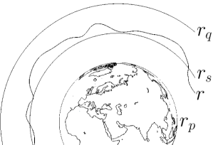
Figure 1: Schematic of the geometry considered in this paper (not to scale). The variable satellite locations $r$, with a representative value ${r_{s}}$, lie between the planetary surface approximated by the sphere of radius ${r_{p}}$ and an outer sphere of radius ${r_{q}}$. The spherical shell $\circledcirc$ between ${r_{p}}$ and ${r_{q}}$ is assumed source-free.

2.2 Vector spherical harmonics for vector fields

Many satellite instruments do not measure the scalar potential fields $V$ and $W$ directly, but rather the vector field $\boldsymbol{B}$ (e.g., the magnetic field or gravitational force) of their superposition, namely

$$\boldsymbol{B}(r\boldsymbol{\hat{r}})=\mbox{\boldmath$\nabla$}V(r\boldsymbol{\hat{r}})+\mbox{\boldmath$\nabla$}W(r\boldsymbol{\hat{r}}).$$ (12)

Using $\mbox{\boldmath$\nabla$}=\boldsymbol{\hat{r}}\hskip 1.00006pt\partial_{r}+r^{-1}\mbox{\boldmath$\nabla$}_{1}$, and $\mbox{\boldmath$\nabla$}_{1}=\boldsymbol{\hat{\theta}}\hskip 1.00006pt\partial_{\theta}+\boldsymbol{\hat{\phi}}\hskip 1.00006pt(\sin\theta)^{-1}\partial_{\phi}$, we express the gradients of the potentials in eqs (4)–(5) in eq. (12) as

$$\mbox{\boldmath$\nabla$}V(r\boldsymbol{\hat{r}}) =\sum_{l=0}^{\infty}\sum_{m=-l}^{l}-{r_{p}^{-1}}\left(\frac{r}{{r_{p}}}\right)^{-l-2}v^{r_{p}}_{lm}\Big{[}\boldsymbol{\hat{r}}\hskip 1.00006pt(l+1)Y_{lm}(\boldsymbol{\hat{r}})-\mbox{\boldmath$\nabla$}_{1}Y_{lm}(\boldsymbol{\hat{r}})\Big{]},$$ (13)

$$\mbox{\boldmath$\nabla$}W(r\boldsymbol{\hat{r}}) =\sum_{l=1}^{\infty}\sum_{m=-l}^{l}{r_{q}^{-1}}\left(\frac{r}{{r_{q}}}\right)^{l-1}w^{r_{q}}_{lm}\Big{[}\boldsymbol{\hat{r}}\hskip 1.00006ptlY_{lm}(\boldsymbol{\hat{r}})+\mbox{\boldmath$\nabla$}_{1}Y_{lm}(\boldsymbol{\hat{r}})\Big{]}.$$ (14)

In eqs (13)–(14), the expressions in the square brackets are vector-valued spherical harmonic functions. We jointly orthonormalize them over the unit sphere and name them

$$\boldsymbol{E}_{lm}(\boldsymbol{\hat{r}}) =\frac{1}{\sqrt{(l+1)(2l+1)}}\Big{[}\boldsymbol{\hat{r}}\hskip 1.00006pt(l+1)Y_{lm}(\boldsymbol{\hat{r}})-\mbox{\boldmath$\nabla$}_{1}Y_{lm}(\boldsymbol{\hat{r}})\Big{]},$$ (15)

$$\boldsymbol{F}_{lm}(\boldsymbol{\hat{r}}) =\frac{1}{\sqrt{l(2l+1)}}\Big{[}\boldsymbol{\hat{r}}\hskip 1.00006ptlY_{lm}(\boldsymbol{\hat{r}})+\mbox{\boldmath$\nabla$}_{1}Y_{lm}(\boldsymbol{\hat{r}})\Big{]}.$$ (16)

With the help of eqs (15)–(16) we rewrite eqs (13)–(14) succinctly in a form amenable to up- and downward continuation within the shell $\circledcirc$,

$$\mbox{\boldmath$\nabla$}V(r\boldsymbol{\hat{r}}) =\sum_{l=0}^{\infty}\sum_{m=-l}^{l}A_{l}(r)\,v^{r_{p}}_{lm}\,\boldsymbol{E}_{lm}(\boldsymbol{\hat{r}})\quad\mbox{where}\quad A_{l}(r)=-{r_{p}^{-1}}\sqrt{(l+1)(2l+1)}\left(\frac{r}{{r_{p}}}\right)^{-l-2},$$ (17)

$$\mbox{\boldmath$\nabla$}W(r\boldsymbol{\hat{r}}) =\sum_{l=1}^{\infty}\sum_{m=-l}^{l}\breve{A}_{l}(r)\,w^{r_{q}}_{lm}\,\boldsymbol{F}_{lm}(\boldsymbol{\hat{r}})\quad\mbox{where}\quad\breve{A}_{l}(r)={r_{q}^{-1}}\sqrt{l(2l+1)}\left(\frac{r}{{r_{q}}}\right)^{l-1}.$$ (18)

None of our formulations used ‘toroidal’ vector harmonics, the $\boldsymbol{C}_{lm}$ of Dahlen and Tromp (1998) or Plattner and Simons (2014, 2015b). These do not result from potential-field gradients and cannot be analytically continued as the expressions containing $\boldsymbol{E}_{lm}$ and $\boldsymbol{F}_{lm}$. Any of their contributions to our data will be disregarded as unmodelable components. Where necessary we expand the degree-dependent harmonic continuation operators $A_{l}(r)$ and $\breve{A}_{l}(r)$ to a ‘full’ form, defining ‘stretchable’ diagonal matrices, whose dimensions depend on the context,

$$\mathbf{A}(r) \quad\mbox{with elements}\quad A_{lm,l^{\prime}m^{\prime}}(r)=A_{l}(r)\,\delta_{ll^{\prime}}\delta_{mm^{\prime}},$$ (19)

$$\mathbf{\breve{A}}(r) \quad\mbox{with elements}\quad\breve{A}_{lm,l^{\prime}m^{\prime}}(r)=\breve{A}_{l}(r)\,\delta_{ll^{\prime}}\delta_{mm^{\prime}},$$ (20)

and when we suppress their argument, we shall mean $r={r_{s}}$, using the ‘silent’ notation

$$\mathbf{A} \quad\mbox{with elements}\quad A_{lm,l^{\prime}m^{\prime}}=A_{l}({r_{s}})\,\delta_{ll^{\prime}}\delta_{mm^{\prime}},$$ (21)

$$\mathbf{\breve{A}} \quad\mbox{with elements}\quad\breve{A}_{lm,l^{\prime}m^{\prime}}=\breve{A}_{l}({r_{s}})\,\delta_{ll^{\prime}}\delta_{mm^{\prime}}.$$ (22)

As with eq. (7), we define the infinite-dimensional vectors $\boldsymbol{\mathcal{E}}$ and $\boldsymbol{\mathcal{F}}$ to comprise all functions $\boldsymbol{E}_{lm}$ and $\boldsymbol{F}_{lm}$, but partition them into bandlimited subsets, $\boldsymbol{\mathcal{E}}_{L}$ and $\boldsymbol{\mathcal{F}}_{L_{o}}$, and their infinite-dimensional complements, $\boldsymbol{\mathcal{E}}_{>L}$ and $\boldsymbol{\mathcal{F}}_{>{L_{o}}}$,

$$\boldsymbol{\mathcal{E}}=\begin{pmatrix}\boldsymbol{\mathcal{E}}^{\mathcal{T}}_{L}\quad\boldsymbol{\mathcal{E}}^{\mathcal{T}}_{>L}\end{pmatrix}^{\mathcal{T}}\quad\mbox{and}\quad\boldsymbol{\mathcal{F}}=\begin{pmatrix}\boldsymbol{\mathcal{F}}^{\mathcal{T}}_{L_{o}}\quad\boldsymbol{\mathcal{F}}^{\mathcal{T}}_{>{L_{o}}}\end{pmatrix}^{\mathcal{T}},$$ (23)

where, as in eq. (8), we write out the pieces containing the $\boldsymbol{E}_{lm}$ for $0\leq l\leq L$, and the $\boldsymbol{F}_{lm}$ for $1\leq l\leq{L_{o}}$, as follows,

$$\boldsymbol{\mathcal{E}}_{L}=\begin{pmatrix}\boldsymbol{E}_{00}&\cdots&\boldsymbol{E}_{lm}&\cdots&\boldsymbol{E}_{LL}\end{pmatrix}^{T}\quad\mbox{and}\quad\boldsymbol{\mathcal{F}}_{L_{o}}=\begin{pmatrix}\boldsymbol{F}_{1\,-1}&\cdots&\boldsymbol{F}_{lm}&\cdots&\boldsymbol{F}_{{L_{o}}{L_{o}}}\end{pmatrix}^{T}.$$ (24)

We arrive at the useful shorthand for eqs (17)–(18), evaluated at a common radius ${r_{s}}$, in the form

$$\mbox{\boldmath$\nabla$}V({r_{s}}\boldsymbol{\hat{r}}) =\boldsymbol{\mathcal{E}}_{L}^{\mathcal{T}}\mathbf{A}^{\mathrm{T}}\mathrm{v}_{L}^{r_{p}}+\boldsymbol{\mathcal{E}}_{>L}^{\mathcal{T}}\mathbf{A}^{\mathrm{T}}\mathrm{v}^{r_{p}}_{>L},$$ (25)

$$\mbox{\boldmath$\nabla$}W({r_{s}}\boldsymbol{\hat{r}}) =\boldsymbol{\mathcal{E}}_{L_{o}}^{\mathcal{T}}\mathbf{\breve{A}}^{\mathrm{T}}\mathrm{w}_{L_{o}}^{r_{q}}+\boldsymbol{\mathcal{F}}_{>{L_{o}}}^{\mathcal{T}}\mathbf{\breve{A}}^{\mathrm{T}}\mathrm{w}^{r_{q}}_{>{L_{o}}}.$$ (26)

We use the symbol $\cdot$ to denote the inner products applied to each element pair of the vector or matrix of vector-valued functions, e.g.,

$$\boldsymbol{\mathcal{E}}_{L}\cdot\boldsymbol{\mathcal{E}}_{L}^{\mathcal{T}}=\begin{pmatrix}\boldsymbol{E}_{00}\cdot\boldsymbol{E}_{00}&\cdots&\boldsymbol{E}_{00}\cdot\boldsymbol{E}_{LL}\\ \vdots&&\vdots\\ \boldsymbol{E}_{LL}\cdot\boldsymbol{E}_{00}&\cdots&\boldsymbol{E}_{LL}\cdot\boldsymbol{E}_{LL}\end{pmatrix}\quad\mbox{and}\quad\boldsymbol{\mathcal{E}}_{L}\cdot\boldsymbol{\mathcal{F}}_{L_{o}}^{\mathcal{T}}=\begin{pmatrix}\boldsymbol{E}_{00}\cdot\boldsymbol{F}_{1\,-1}&\cdots&\boldsymbol{E}_{00}\cdot\boldsymbol{F}_{{L_{o}}{L_{o}}}\\ \vdots&&\vdots\\ \boldsymbol{E}_{LL}\cdot\boldsymbol{F}_{1\,-1}&\cdots&\boldsymbol{E}_{LL}\cdot\boldsymbol{F}_{{L_{o}}{L_{o}}}\end{pmatrix}.$$ (27)

and likewise for future combinations of $\boldsymbol{\mathcal{E}}$ and $\boldsymbol{\mathcal{F}}$, subscripted or not. Hence, the joint orthonormality leads to expressions of the form

$$\int_{\Omega}\boldsymbol{\mathcal{E}}\cdot\boldsymbol{\mathcal{E}}^{\mathcal{T}}d\Omega=\mathbf{I},\qquad\int_{\Omega}\boldsymbol{\mathcal{F}}\cdot\boldsymbol{\mathcal{F}}^{\mathcal{T}}d\Omega=\mathbf{I},\quad\mbox{and}\quad\int_{\Omega}\boldsymbol{\mathcal{E}}\cdot\boldsymbol{\mathcal{F}}^{\mathcal{T}}d\Omega=\mathbf{0}.$$ (28)

3 Statement of the problem

When estimating planetary gravity or magnetic fields from sources within a planet we assume that the spherical shell $\circledcirc$ between the planetary surface and the upper limit of our satellite data altitude is free of any field sources. This allows us to downward-continue the coefficients for the potential fields at $r$ onto the planetary surface ${r_{p}}$, or upward-continue them to the outer range of the spherical shell ${r_{q}}$, per eqs (17)–(18).

The measured data are a superposition of the fields from internal and external sources, and contributions collected in a noise term,

$$\boldsymbol{d}(r\boldsymbol{\hat{r}})=\begin{cases}\mbox{\boldmath$\nabla$}V(r\boldsymbol{\hat{r}})+\mbox{\boldmath$\nabla$}W(r\boldsymbol{\hat{r}})+\boldsymbol{n}(r\boldsymbol{\hat{r}})&\text{if }\boldsymbol{\hat{r}}\in R\subset\Omega,\\ \text{unknown}&\text{if }\boldsymbol{\hat{r}}\in\Omega\setminus R,\end{cases}$$ (29)

Our goal is to obtain, from discrete satellite data collected within a confined region $R$ at varying altitude above the planetary surface approximated by a sphere of radius ${r_{p}}$, the bandlimited set of coefficients $v^{r_{p}}_{lm}\in\mathrm{v}_{L}^{r_{p}}$, $0\leq l\leq L$, that describe $V$ on the planetary surface. We will discuss two versions of this problem. In the first, treated in Section 4, we remove the external field from consideration. In the second, discussed in Section 5, we solve simultaneously also for the external-field coefficients that describe the potential $W$, recovering as best we can the $w^{r_{q}}_{lm}\in\mathrm{w}_{L_{o}}^{r_{q}}$, $1\leq l\leq{L_{o}}$. As made explicit via eq. (6), we will be forming strictly bandlimited estimates of the broadband fields $\mbox{\boldmath$\nabla$}V$ and $\mbox{\boldmath$\nabla$}W$ in eqs (17)–(18), up to a certain $L$ and ${L_{o}}$, not necessarily identical, for the internal and external fields, respectively. In Sections 9 and 10 we will be quantifying the broadband bias that is the inevitable result of such choices.

In our formulation of the problem in eq. (29), we assume static data with any time variation collected in the noise term. To avoid temporal aliasing the data might be binned by time stamp, and each bin inverted individually.

4 Solution by the internal-field altitude-cognizant GVSF method

When we ignore the external field, either because it is deemed insignificant, or because we modeled and subtracted it from the data, the term containing $W$ in eq. (12) vanishes. For example, Plattner and Simons (2015a) subtracted a model of the external nighttime field for Mars obtained by Olsen et al. (2010b) and assumed no further external-field contribution. In this section we detail the Plattner and Simons (2015a) construction of a Slepian basis of functions to serve as an effective lesser-dimensional alternative to the vector spherical harmonics for inverse modeling of the internal potential field $V$ from vector data at satellite altitude. These internal-field altitude-cognizant gradient vector Slepian functions (AC-GVSF) take into account the region of data availability $R$, the radial coordinate of data acquisition $r$, and the resolvable spherical-harmonic bandwidth $L$. The present section is only concerned with the construction of the basis functions; the next section deals with their usage in realistic data analysis settings.

4.1 Restatement of the inverse problem

For the construction of the localized function basis we assume that the data exist as a continuous function on the sphere of radius ${r_{s}}$. Avoiding for now the specification of discrete data locations, the only manner in which the new basis construction depends on the data is through the boundary of their geographic region of availability, and the satellite altitude that is representative for them. For regions with rotational symmetry the construction will then be computationally very efficient, as we discuss in Appendix A.1. Within the region $R$ the vector-valued satellite data $\boldsymbol{d}({r_{s}}\boldsymbol{\hat{r}})$ are the sum of the vector-valued gradient of the unknown scalar-potential internal field and a noise term,

$$\boldsymbol{d}({r_{s}}\boldsymbol{\hat{r}})=\begin{cases}\mbox{\boldmath$\nabla$}V({r_{s}}\boldsymbol{\hat{r}})+\boldsymbol{n}({r_{s}}\boldsymbol{\hat{r}})&\text{if~{}}\boldsymbol{\hat{r}}\in R,\\ \text{unknown}&\text{if~{}}\boldsymbol{\hat{r}}\in\Omega\setminus R.\end{cases}$$ (30)

We will be using the ‘silent’ notation whereby $\boldsymbol{d}=\boldsymbol{d}({r_{s}}\boldsymbol{\hat{r}})$. As is clear from eq. (17), in terms of the unit-sphere harmonics $\boldsymbol{E}_{lm}(\boldsymbol{\hat{r}})$, the coefficients $v^{r_{p}}_{lm}$ that describe the internal potential field on the planetary surface ${r_{p}}$ relate to the ones describing that same field at some average satellite radius ${r_{s}}$ via a upward-continuation transformation that we write in terms of the diagonal matrix $\mathbf{A}$ defined in eq. (21). In the notation developed in Section 2, this allows us to rewrite the bandlimited portion of the vector field that we attempt to recover, for a fixed average satellite orbital radius ${r_{s}}$, in terms of the vector spherical harmonic basis functions $\mathbf{A}\boldsymbol{\mathcal{E}}_{L}$, and with that, we define a solution as the least-squares minimizer

$$\mathrm{\tilde{v}}^{r_{p}}_{L}=\arg\min_{\mathrm{v}_{L}^{r_{p}}}\left\{\int_{R}\left(\boldsymbol{\mathcal{E}}_{L}^{\mathcal{T}}\mathbf{A}^{\mathrm{T}}\mathrm{v}_{L}^{r_{p}}-\boldsymbol{d}\right)^{2}d\Omega\right\}.$$ (31)

We solve eq. (31) by calculating the derivative with respect to the coefficient vector $\mathrm{v}_{L}^{r_{p}}$ and setting the result equal to zero to obtain

$$\mathbf{A}\left(\int_{R}\boldsymbol{\mathcal{E}}_{L}\cdot\boldsymbol{\mathcal{E}}_{L}^{\mathcal{T}}d\Omega\right)\mathbf{A}^{\mathrm{T}}\mathrm{\tilde{v}}_{L}^{r_{p}}=\mathbf{A}\int_{R}\boldsymbol{\mathcal{E}}_{L}\cdot\boldsymbol{d}\,d\Omega.$$ (32)

In the dot product notation of eq. (27),

$$\boldsymbol{\mathcal{E}}_{L}\cdot\boldsymbol{d}=\begin{pmatrix}\boldsymbol{E}_{00}\cdot\boldsymbol{d}&\cdots&\boldsymbol{E}_{lm}\cdot\boldsymbol{d}&\cdots&\boldsymbol{E}_{LL}\cdot\boldsymbol{d}\end{pmatrix}^{T}.$$ (33)

4.2 A Slepian approach to the internal-field problem

Eq. (32) is linear in the data. As did Plattner and Simons (2015a) we define the symmetric positive-definite matrix

$$\mathbf{K}=\mathbf{A}\left(\int_{R}\boldsymbol{\mathcal{E}}_{L}\cdot\boldsymbol{\mathcal{E}}_{L}^{\mathcal{T}}d\Omega\right)\,\mathbf{A}^{\mathrm{T}}.$$ (34)

At large bandwidths $L$ and for high satellite altitudes ${r_{s}}$, the $(L+1)^{2}\times(L+1)^{2}$-dimensional matrix $\mathbf{K}$ is poorly conditioned, and solving the system (32) via matrix inversion to obtain $\mathrm{\tilde{v}}_{L}^{r_{p}}$ requires regularization. Under a Tikhonov numerical scheme we would add a suitably regular matrix to $\mathbf{K}$ prior to inversion, which, in a Bayesian interpretation is akin to supplying a priori information Aster et al. (2013). Approaching the problem via singular value decomposition (SVD), we focus on solving for the well-conditioned components of problem (32). Working from the eigenvector decomposition of $\mathbf{K}$ we will rewrite the solution in terms of those eigenvectors that have relatively large eigenvalues, and then we will solve for their expansion coefficients. When the region $R$ is an arbitrary geographical domain, and when $L$ is large, the eigendecomposition will be costly, but in Appendix A.1 we show that for regions with special symmetry, $\mathbf{K}$ can be transformed into a block-diagonal matrix with a maximal block size of $(L+1)\times(L+1)$, which significantly reduces its diagonalization cost.

The eigenvectors of the real-valued Hermitian matrix $\mathbf{K}$ are orthogonal. We orthonormalize the eigenvectors, hence we write

$$\mathbf{K}\mathbf{G}=\mathbf{G}\mathbf{\Lambda},\quad\mbox{where}\quad\mathbf{G}^{\mathrm{T}}\mathbf{G}=\mathbf{I}_{(L+1)^{2}}=\mathbf{G}\mathbf{G}^{\mathrm{T}},$$ (35)

where $\mathbf{\Lambda}$ is the diagonal matrix of sorted real-valued eigenvalues $1>\lambda_{1}\geq\lambda_{2}\geq\cdots\geq\lambda_{(L+1)^{2}}>0$, and $\mathbf{I}$ the identity. The columns of the $(L+1)^{2}\times(L+1)^{2}$-dimensional matrix $\mathbf{G}$ are the eigenvectors of $\mathbf{K}$. The matrix $\mathbf{G}_{J}$ is the $(L+1)^{2}\times{J}$-dimensional restriction to its first ${J}$ columns, thus the untruncated $\mathbf{G}=\mathbf{G}_{(L+1)^{2}}$, and $\mathbf{G}_{>{J}}$ will be the complement to $\mathbf{G}_{J}$. We note right away that

$$\mathbf{K}\mathbf{G}_{J}=\mathbf{G}_{J}\mathbf{\Lambda}_{J},\quad\mbox{where}\quad\mathbf{G}_{J}^{\mathrm{T}}\mathbf{G}_{J}=\mathbf{I}_{J},\quad\mbox{but}\quad\left(\mathbf{G}_{J}\mathbf{G}_{J}^{\mathrm{T}}\right)^{n}=\mathbf{G}_{J}\mathbf{G}_{J}^{\mathrm{T}}\neq\mathbf{I}_{(L+1)^{2}},$$ (36)

for any positive integer $n$, is a non-invertible projection except for $R=\Omega$. We do note that $\mathbf{G}_{J}\mathbf{G}_{J}^{\mathrm{T}}+\mathbf{G}_{>{J}}\mathbf{G}_{>{J}}^{\mathrm{T}}=\mathbf{I}_{(L+1)^{2}}$. Each of the columns of $\mathbf{G}$, which we denote $\mathrm{g}_{\alpha}$ and arrange as

$$\mathbf{G}=\begin{pmatrix}\mathrm{g}_{1}&\cdots&\mathrm{g}_{\alpha}&\cdots&\mathrm{g}_{(L+1)^{2}}\end{pmatrix}=\begin{pmatrix}\mathbf{G}_{J}\quad\mathbf{G}_{>{J}}\end{pmatrix},\quad\mbox{where}\quad\mathbf{G}_{J}=\begin{pmatrix}\mathrm{g}_{1}&\cdots&\mathrm{g}_{\alpha}&\cdots&\mathrm{g}_{J}\end{pmatrix},$$ (37)

contains a spherical-harmonic coefficient set $\mathrm{g}_{\alpha}=\begin{pmatrix}g_{00,\alpha}&\cdots&g_{lm,\alpha}&\cdots&g_{LL,\alpha}\end{pmatrix}^{T}$, with a power spectrum or mean-squared value

$$\mathscr{G}_{\alpha}(l)=\frac{1}{2l+1}\sum_{m=-l}^{l}g_{lm,\alpha}^{2}.$$ (38)

In what follows we take pains to distinguish ‘light’ and ‘bold’, uncapitalized and capitalized, roman ($\mathrm{g}$, $\mathbf{G}$), italicized ($g$, $G$, $\boldsymbol{G}$), calligraphic ($\mathcal{G}$, $\boldsymbol{\mathcal{G}}$) or script ($\mathscr{G}$) fonts, depending on whether the quantity of interest is a column vector or a matrix, a scalar function or a vector function, a column vector of scalar functions or of vector functions, or a power-spectrum, respectively — exactly as in Section 2, where we had already encountered $\mathrm{v}$, $\mathbf{A}$, $v$, $V$, $\boldsymbol{E}$, $\mathcal{Y}$, and $\boldsymbol{\mathcal{E}}$, for example. We will furthermore see that $g_{lm,\alpha}\in\mathrm{g}_{\alpha}\subset\mathbf{G}$, $G_{\alpha}\in\mathcal{G}$, $\boldsymbol{G}_{\alpha}\in\boldsymbol{\mathcal{G}}$, and so on.

We use the internal-field altitude-cognizant Slepian transform in three distinct ways.

[1] Expanded in scalar spherical harmonics in the coordinates of the unit sphere, we define an altitude-cognizant scalar Slepian function,

$$G_{\alpha}(\boldsymbol{\hat{r}})=\sum_{l=0}^{L}\sum_{m=-l}^{l}g_{lm,\alpha}Y_{lm}(\boldsymbol{\hat{r}}).$$ (39)

With the help of eq. (8), we use eqs (37) and (39) to define the column vector of such functions $G_{\alpha}(\boldsymbol{\hat{r}})=\mathcal{Y}_{L}^{\mathcal{T}}\mathrm{g}_{\alpha}$,

$$\mathcal{G}_{J}=\begin{pmatrix}G_{1}&\cdots&G_{\alpha}&\cdots&G_{J}\end{pmatrix}^{T}=\mathbf{G}^{\mathrm{T}}_{J}\mathcal{Y}_{L},\quad\mbox{with}\quad 1\leq{J}\leq(L+1)^{2}.$$ (40)

We partition the full set as $\mathcal{G}=\mathcal{G}_{(L+1)^{2}}=(\mathcal{G}_{J}^{\mathcal{T}}\quad\mathcal{G}_{>{J}}^{\mathcal{T}})^{\mathcal{T}}$, whereby $\mathcal{G}^{\mathcal{T}}\mathcal{G}=\mathcal{G}_{{J}}^{\mathcal{T}}\mathcal{G}_{{J}}+\mathcal{G}_{>{J}}^{\mathcal{T}}\mathcal{G}_{>{J}}=\mathcal{Y}^{\mathcal{T}}_{L}\mathcal{Y}_{L}$.

[2] When expanded into the vector spherical-harmonic basis on the planetary sphere of radius ${r_{p}}$, every eigenvector $\mathrm{g}_{\alpha}$ yields an altitude-cognizant gradient vector Slepian function (AC-GVSF),

$$\boldsymbol{G}_{\alpha}({r_{p}}\boldsymbol{\hat{r}})=\sum_{l=0}^{L}\sum_{m=-l}^{l}A_{l}({r_{p}})\,g_{lm,\alpha}\,\boldsymbol{E}_{lm}(\boldsymbol{\hat{r}}).$$ (41)

In the same vein as eq. (40), using eqs (24), (37) and (41), we write the vector containing those functions $\boldsymbol{G}_{\alpha}({r_{p}}\boldsymbol{\hat{r}})=\boldsymbol{\mathcal{E}}_{L}^{\mathcal{T}}\mathbf{A}({r_{p}})\,\mathrm{g}_{\alpha}$,

$$\boldsymbol{\mathcal{G}}_{J}=\begin{pmatrix}\boldsymbol{G}_{1}&\cdots&\boldsymbol{G}_{\alpha}&\cdots&\boldsymbol{G}_{J}\end{pmatrix}^{T}=\mathbf{G}^{\mathrm{T}}_{J}\mathbf{A}({r_{p}})\,\boldsymbol{\mathcal{E}}_{L},\quad\mbox{with}\quad 1\leq{J}\leq(L+1)^{2},$$ (42)

again partitioned as $\boldsymbol{\mathcal{G}}=\boldsymbol{\mathcal{G}}_{(L+1)^{2}}=(\boldsymbol{\mathcal{G}}^{\mathcal{T}}_{J}\quad\boldsymbol{\mathcal{G}}^{\mathcal{T}}_{>{J}})^{\mathcal{T}}$.

[3] At satellite altitude ${r_{s}}$, we define a vector of upward-continued AC-GVSF in the ‘silent’ notation $\boldsymbol{G}_{\uparrow\alpha}({r_{s}}\boldsymbol{\hat{r}})=\boldsymbol{\mathcal{E}}_{L}^{\mathcal{T}}\mathbf{A}\,\mathrm{g}_{\alpha}$,

$$\boldsymbol{\mathcal{G}}_{\uparrow{J}}=\begin{pmatrix}\boldsymbol{G}_{\uparrow 1}&\cdots&\boldsymbol{G}_{\uparrow\alpha}&\cdots&\boldsymbol{G}_{\uparrow{J}}\end{pmatrix}^{T}=\mathbf{G}_{J}^{\mathrm{T}}\mathbf{A}\,\boldsymbol{\mathcal{E}}_{L},\quad\mbox{with}\quad 1\leq{J}\leq(L+1)^{2}.$$ (43)

We maintain the usual partition $\boldsymbol{\mathcal{G}}_{\uparrow}=\boldsymbol{\mathcal{G}}_{\uparrow(L+1)^{2}}=(\boldsymbol{\mathcal{G}}^{\mathcal{T}}_{\uparrow{J}}\quad\boldsymbol{\mathcal{G}}^{\mathcal{T}}_{\uparrow>{J}})^{\mathcal{T}}$.

Whatever the region of concentration $R$, owing to the orthogonality of the transformation (35)–(40), the entire ${J}=(L+1)^{2}$-dimensional untruncated set of scalar Slepian functions remains a complete basis for bandlimited internal-potential functions. On the planetary surface ${r_{p}}$,

$$\mathcal{Y}_{L}^{\mathcal{T}}\mathrm{v}_{L}^{r_{p}}=\mathcal{Y}_{L}^{\mathcal{T}}\left(\mathbf{G}\mathbf{G}^{\mathrm{T}}\right)\mathrm{v}_{L}^{r_{p}}=\left(\mathbf{G}^{\mathrm{T}}\mathcal{Y}_{L}\right)^{\mathrm{T}}\left(\mathbf{G}^{\mathrm{T}}\mathrm{v}_{L}^{r_{p}}\right)=\mathcal{G}^{\mathcal{T}}\mathrm{s}.$$ (44)

The expansion coefficients of a bandlimited potential field at ${r_{p}}$, e.g. $v^{r_{p}}_{lm}$ in the scalar spherical-harmonic basis $Y_{lm}(\boldsymbol{\hat{r}})$, transform to the coefficients of a scalar Slepian basis $G_{\alpha}(\boldsymbol{\hat{r}})$, designed with the same bandwidth $L$ but for whichever region $R$, as

$$s_{\alpha} =\int_{\Omega}V({r_{p}}\boldsymbol{\hat{r}})\,G_{\alpha}(\boldsymbol{\hat{r}})\,d\Omega=\sum_{l=0}^{L}\sum_{m=-l}^{l}g_{lm,\alpha}\,v^{r_{p}}_{lm}\quad\text{or, in vector form,}$$ (45)

$$\mathrm{s}_{J} =\int_{\Omega}V({r_{p}}\boldsymbol{\hat{r}})\,\mathcal{G}_{{J}}(\boldsymbol{\hat{r}})\,d\Omega=\mathbf{G}_{J}^{\mathrm{T}}\mathrm{v}_{L}^{r_{p}},\quad\mbox{with}\quad 1\leq{J}\leq(L+1)^{2}.$$ (46)

The crux of our inversion method will rely on the property that a $J<(L+1)^{2}$-dimensional truncated subset of high-eigenvalue Slepian functions will remain an approximate basis for functions considered over a confined geographical domain $R$, if it matches the region for which the Slepian functions were designed, and for the same bandlimit $L$, in the sense that $\int_{R}(\mathcal{G}_{J}^{\mathcal{T}}\mathrm{s}_{J}-\mathcal{G}^{\mathcal{T}}\mathrm{s})^{2}\,d\Omega$ will be small for suitable ${J}$.

Fig. 2 shows the radial, colatitudinal, and longitudinal components of the highest-eigenvalue internal-field AC-GVSF for a planetary radius ${r_{p}}=6371$ km, a satellite radius ${r_{s}}=6671$ km, region $R=$ North America, and maximum spherical-harmonic degree $L=100$. Shown are the vector components $\boldsymbol{G}_{1}\cdot\boldsymbol{\hat{r}}$, $\boldsymbol{G}_{1}\cdot\boldsymbol{\hat{\theta}}$, and $\boldsymbol{G}_{1}\cdot\boldsymbol{\hat{\phi}}$, with their power spectrum $\mathscr{G}_{1}$. Even though the function $\boldsymbol{G}_{1}$ has a bandwidth $L=100$, the spatial pattern in Fig. 2 is consistent with an effective bandwidth that is much lower, as also seen in the power spectrum. Herein lies the difference of the AC-GVSF, first developed by Plattner and Simons (2015a), with the ‘classical’ gradient vector Slepian functionfunctions (CL-GVSF) of Plattner and Simons (2015b), which did not incorporate the upward-continuation operators $A_{lm,l^{\prime}m^{\prime}}$ of eq. (19) into the optimization solution of eq. (32), which now leads to the diagonalization of the matrix $\mathbf{K}$ in eq. (34). The eigenvector with the largest eigenvalue in eq. (35) displays only small but non-zero coefficients at the highest spherical-harmonic degrees. Since information at those degrees is more sensitive to noise amplification under downward-continuation, this was to be expected. It is furthermore reflected in the power spectrum in Fig. 2, where the spherical-harmonic degrees higher than about $l=40$ are characterized by very low power.

Fig. 3 shows the three components of the 100th best-concentrated internal-field AC-GVSF for the same parameters as in Fig. 2. The function values of $\boldsymbol{G}_{100}$ reveal much finer structures than those of $\boldsymbol{G}_{1}$ in Fig. 2, and the spectrum $\mathscr{G}_{100}$ manifests more power at the higher spherical-harmonic degrees than did $\mathscr{G}_{1}$ in Fig. 2. The increased power at the higher spherical-harmonic degrees of the lower-eigenvalue AC-GVSF is in principle accompanied by the ability to resolve finer spatial details. However, in the data analysis these functions might also be more prone than the lower-ranked internal-field AC-GVSF to fitting noise rather than signal.

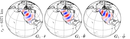
Figure 2: The best-concentrated (highest-eigenvalue) internal-field altitude-cognizant gradient vector Slepian function (AC-GVSF) $\boldsymbol{G}_{1}$, as from eq. (41), for region $R=$ North America, ${r_{p}}=6371$ km, ${r_{s}}=6671$ km (i.e. at 300 km satellite altitude), and bandwidth $L=100$. Top row: vector (radial, colatitudinal, and longitudinal) components of the AC-GVSF evaluated on the planetary surface. Bottom panel: the power spectrum $\mathscr{G}_{1}$, from eq. (38).

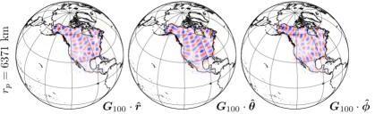
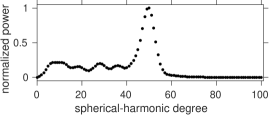
Figure 3: The 100th-best concentrated internal-field AC-GVSF, $\boldsymbol{G}_{100}$, and its power spectrum, $\mathscr{G}_{100}$, for the same parameters and layout as in Fig. 2.

4.3 Continuous solution by internal-field altitude-cognizant GVSF

With the help of eqs (34)–(35) and the orthogonality of the matrix $\mathbf{G}$, the problem (32) is rewritten as

$$\mathbf{K}\,\mathrm{\tilde{v}}_{L}^{r_{p}}=\mathbf{G}\mathbf{\Lambda}\mathbf{G}^{\mathrm{T}}\mathrm{\tilde{v}}_{L}^{r_{p}}=\mathbf{A}\int_{R}\boldsymbol{\mathcal{E}}_{L}\cdot\boldsymbol{d}\,d\Omega.$$ (47)

We implement the truncated-SVD approach in using the first ${J}$ columns of the matrix $\mathbf{G}$, hence, using the formalism of eqs (36) and (46),

$$\mathbf{G}_{J}\mathbf{\Lambda}_{J}\,\tilde{\mathrm{s}}_{{J}}=\mathbf{A}\int_{R}\boldsymbol{\mathcal{E}}_{L}\cdot\boldsymbol{d}\,d\Omega,$$ (48)

where $\mathbf{G}_{J}$ is as in eq. (37), and $\mathbf{\Lambda}_{J}$ is the diagonal matrix consisting of the ${J}$ largest eigenvalues $\lambda_{1}\geq\cdots\geq\lambda_{{J}}>0$ of $\mathbf{K}$. The new version, eq. (48), is not identical to the original problem, eq. (47), given eq. (36), and $\tilde{\mathrm{s}}_{{J}}$ is a truncated Slepian-transform estimator. The value for the regularization parameter ${J}$ remains to be chosen. If we select ${J}$ such that all eigenvalues $\lambda_{\alpha}$ are similar in magnitude, the system (48) will be well conditioned, and can be solved by the left-inverse of $\mathbf{G}_{J}\mathbf{\Lambda}_{J}$, which is $\mathbf{\Lambda}^{-1}\mathbf{G}_{J}^{\mathrm{T}}$, per eq. (36). This defines a solution, using eq. (43),

$$\tilde{\mathrm{s}}_{{J}}=\mathbf{\Lambda}_{J}^{-1}\int_{R}\boldsymbol{\mathcal{G}}_{\uparrow{J}}\cdot\boldsymbol{d}\,d\Omega.$$ (49)

The ${J}$-dimensional vector of coefficients $\tilde{\mathrm{s}}_{{J}}$ can be back-projected into the $(L+1)^{2}$-dimensional space of internal-field vector spherical-harmonic coefficients by multiplying it with the $(L+1)^{2}\times{J}$-dimensional matrix $\mathbf{G}_{J}$. We can expand the estimated potential field on the planetary surface from this back-projection, with the help of eq. (40), to form the space-domain estimate

$$\tilde{V}_{J}({r_{p}}\boldsymbol{\hat{r}})=\sum_{\alpha=1}^{J}\tilde{s}_{\alpha}\,G_{\alpha}(\boldsymbol{\hat{r}})=\mathcal{Y}_{L}^{\mathcal{T}}\mathbf{G}_{J}\,\tilde{\mathrm{s}}_{{J}}=\mathcal{G}_{J}^{\mathcal{T}}\,\tilde{\mathrm{s}}_{{J}}.$$ (50)

We note emphatically that the estimator in eq. (50) is different than the one proposed by Plattner and Simons (2015b), their eq. (161), and also briefly discussed by Plattner and Simons (2015a) in their Section 2.2. It is, however, the estimator used by Plattner and Simons (2015a) and discussed in their Section 2.3. The current paper contains the full rationale behind their doing so. The key to the difference is that we use eigenfunctions of eq. (34), which takes the effects of the altitude of the observation into account at the optimization stage.

In this section we described the construction of bandlimited internal-field AC-GVSF, concentrated in a certain region and optimized for a representative satellite altitude. In the following section we expand our method to being able to consider both internal- and external fields.

5 Solution by the full-field altitude-cognizant GVSF method

Modeling both the internal and external fields, i.e, the “full” field from both $V$ and $W$ in eq. (12), with a similar spatio-spectrally localized inversion approach as described in Section 4, requires Slepian functions that contain both internal-field and external-field components.

5.1 Restatement of the inverse problem

As for eq. (30) we assume that the data are a linear combination of a modeled component (signal) and noise, with the signal now containing both the internally and externally generated vector fields,

$$\boldsymbol{d}({r_{s}}\boldsymbol{\hat{r}})=\begin{cases}\mbox{\boldmath$\nabla$}V({r_{s}}\boldsymbol{\hat{r}})+\mbox{\boldmath$\nabla$}W({r_{s}}\boldsymbol{\hat{r}})+\boldsymbol{n}({r_{s}}\boldsymbol{\hat{r}})&\text{if~{}}\boldsymbol{\hat{r}}\in R,\\ \text{unknown}&\text{if~{}}\boldsymbol{\hat{r}}\in\Omega\setminus R.\end{cases}$$ (51)

Complementing the matrix $\mathbf{A}$ that serves to upward-continue the internal-field spherical harmonics, eq. (21), we use the external-field matrix $\mathbf{\breve{A}}$ from eq. (22) to augment eq. (31) to take both fields into account. The internal field is expanded as a linear combination of upward-continued internal-field vector spherical harmonics $\mathbf{A}\boldsymbol{\mathcal{E}}_{L}$, with coefficients $\mathrm{v}_{L}^{r_{p}}$. The external field is a linear combination of upward-continued external-field vector spherical harmonics $\mathbf{\breve{A}}\boldsymbol{\mathcal{F}}_{L_{o}}$, with coefficients $\mathrm{w}_{L_{o}}^{r_{q}}$. The external-field bandwidth, ${L_{o}}$, can be different from the internal-field bandwidth, $L$. We seek a least-squares solution

$$\begin{pmatrix}\displaystyle\mathrm{\tilde{v}}_{L}^{r_{p}}\\ \\ \displaystyle\mathrm{\tilde{w}}_{L_{o}}^{r_{q}}\end{pmatrix}=\arg\min_{\mathrm{v}_{L}^{r_{p}},\mathrm{w}_{L_{o}}^{r_{q}}}\left\{\int_{R}\left(\boldsymbol{\mathcal{E}}_{L}^{\mathcal{T}}\mathbf{A}^{\mathrm{T}}\mathrm{v}_{L}^{r_{p}}+\boldsymbol{\mathcal{F}}_{L_{o}}^{\mathcal{T}}\mathbf{\breve{A}}^{\mathrm{T}}\mathrm{w}_{L_{o}}^{r_{q}}-\boldsymbol{d}\right)^{2}\,d\Omega\right\}.$$ (52)

We solve optimization problem (52) by taking its derivative with respect to the vector $\begin{pmatrix}{\mathrm{v}_{L}^{r_{p}}}^{\mathrm{T}}&{\mathrm{w}_{L_{o}}^{r_{q}}}^{\mathrm{T}}\end{pmatrix}^{\mathrm{T}}$ and setting it to zero. This yields

$$\begin{pmatrix}\displaystyle\mathbf{A}\int_{R}\boldsymbol{\mathcal{E}}_{L}\cdot\boldsymbol{\mathcal{E}}_{L}^{\mathcal{T}}\,d\Omega\,\mathbf{A}^{\mathrm{T}}&\displaystyle\mathbf{A}\int_{R}\boldsymbol{\mathcal{E}}_{L}\cdot\boldsymbol{\mathcal{F}}_{L_{o}}^{\mathcal{T}}\,d\Omega\,\mathbf{\breve{A}}^{\mathrm{T}}\\ &\\ \displaystyle\mathbf{\breve{A}}\int_{R}\boldsymbol{\mathcal{F}}_{L_{o}}\cdot\boldsymbol{\mathcal{E}}_{L}^{\mathcal{T}}\,d\Omega\,\mathbf{A}^{\mathrm{T}}&\displaystyle\mathbf{\breve{A}}\int_{R}\boldsymbol{\mathcal{F}}_{L_{o}}\cdot\boldsymbol{\mathcal{F}}_{L_{o}}^{\mathcal{T}}\,d\Omega\,\mathbf{\breve{A}}^{\mathrm{T}}\end{pmatrix}\begin{pmatrix}\displaystyle\mathrm{\tilde{v}}_{L}^{r_{p}}\\ \\ \displaystyle\mathrm{\tilde{w}}_{L_{o}}^{r_{q}}\end{pmatrix}=\begin{pmatrix}\displaystyle\mathbf{A}\int_{R}\boldsymbol{\mathcal{E}}_{L}\cdot\boldsymbol{d}\,d\Omega\\ \\ \displaystyle\mathbf{\breve{A}}\int_{R}\boldsymbol{\mathcal{F}}_{L_{o}}\cdot\boldsymbol{d}\,d\Omega\end{pmatrix}.$$ (53)

Substituting $\boldsymbol{\mathcal{F}}_{L_{o}}$ for $\boldsymbol{\mathcal{E}}_{L}$, the same dot-product notation as in eqs (27) and (33) is used.

5.2 A Slepian approach to the full-field problem

As with eq. (34) we proceed to regularizing the poorly conditioned linear system (53) by diagonalization of the combined kernel matrix

$$\mathring{\mathbf{K}}=\begin{pmatrix}\displaystyle\mathbf{A}\int_{R}\boldsymbol{\mathcal{E}}_{L}\cdot\boldsymbol{\mathcal{E}}_{L}^{\mathcal{T}}\,d\Omega\,\mathbf{A}^{\mathrm{T}}&\displaystyle\mathbf{A}\int_{R}\boldsymbol{\mathcal{E}}_{L}\cdot\boldsymbol{\mathcal{F}}_{L_{o}}^{\mathcal{T}}\,d\Omega\,\mathbf{\breve{A}}^{\mathrm{T}}\\ &\\ \displaystyle\mathbf{\breve{A}}\int_{R}\boldsymbol{\mathcal{F}}_{L_{o}}\cdot\boldsymbol{\mathcal{E}}_{L}^{\mathcal{T}}\,d\Omega\,\mathbf{A}^{\mathrm{T}}&\displaystyle\mathbf{\breve{A}}\int_{R}\boldsymbol{\mathcal{F}}_{L_{o}}\cdot\boldsymbol{\mathcal{F}}_{L_{o}}^{\mathcal{T}}\,d\Omega\,\mathbf{\breve{A}}^{\mathrm{T}}\end{pmatrix},$$ (54)

which is square, of dimension $[(L+1)^{2}+({L_{o}}+1)^{2}-1]\times[(L+1)^{2}+({L_{o}}+1)^{2}-1]$, and generally fully populated. In Appendix A.2 we show that for symmetric regions the columns and rows of $\mathring{\mathbf{K}}$ can be reordered to a block-diagonal form with the largest block dimension $(L+{L_{o}}+1)\times(L+{L_{o}}+1)$. In the orthogonal eigenvector decomposition of this Hermitian positive definite matrix,

$$\mathring{\mathbf{K}}\mathring{\mathbf{G}}=\mathring{\mathbf{G}}\mathring{\mathbf{\Lambda}},\quad\mbox{where}\quad\mathring{\mathbf{G}}^{\mathrm{T}}\mathring{\mathbf{G}}=\mathbf{I}_{(L+1)^{2}+({L_{o}}+1)^{2}-1}=\mathring{\mathbf{G}}\mathring{\mathbf{G}}^{\mathrm{T}},$$ (55)

the diagonal matrix of eigenvalues $\mathring{\lambda}_{1}\geq\mathring{\lambda}_{2}\geq\cdots\geq\mathring{\lambda}_{(L+1)^{2}+({L_{o}}+1)^{2}-1}>0$ is $\mathring{\mathbf{\Lambda}}$, and $\mathring{\mathbf{G}}$ contains the eigenvectors $\mathring{\mathrm{g}}_{\alpha}$ in the arrangement

$$\mathring{\mathbf{G}}=\begin{pmatrix}\mathring{\mathrm{g}}_{1}&\cdots&\mathring{\mathrm{g}}_{\alpha}&\cdots&\mathring{\mathrm{g}}_{(L+1)^{2}+({L_{o}}+1)^{2}-1}\end{pmatrix}=\begin{pmatrix}\mathring{\mathbf{G}}_{J}\quad\mathring{\mathbf{G}}_{>{J}}\end{pmatrix}\quad\mbox{where}\quad\mathring{\mathbf{G}}_{J}=\begin{pmatrix}\mathring{\mathrm{g}}_{1}&\cdots&\mathring{\mathrm{g}}_{\alpha}&\cdots&\mathring{\mathrm{g}}_{J}\end{pmatrix}.$$ (56)

Again it is to be noted that the relations involving the column restrictions are, for $1\leq{J}\leq(L+1)^{2}+({L_{o}}+1)^{2}-1$ and any $n\in\mathbb{N}$,

$$\mathring{\mathbf{K}}\mathring{\mathbf{G}}_{J}=\mathring{\mathbf{G}}_{J}\mathring{\mathbf{\Lambda}}_{J},\quad\mbox{where}\quad\mathring{\mathbf{G}}_{J}^{\mathrm{T}}\mathring{\mathbf{G}}_{J}=\mathbf{I}_{J},\quad\mbox{but}\quad\left(\mathring{\mathbf{G}}_{J}\mathring{\mathbf{G}}_{J}^{\mathrm{T}}\right)^{n}=\mathring{\mathbf{G}}_{J}\mathring{\mathbf{G}}_{J}^{\mathrm{T}}\neq\mathbf{I}_{(L+1)^{2}+({L_{o}}+1)^{2}-1}.$$ (57)

Each of the column vectors in $\mathring{\mathbf{G}}$ contains coefficients for the internal and the external fields, and $\mathring{\mathbf{G}}=\mathring{\mathbf{G}}_{(L+1)^{2}+({L_{o}}+1)^{2}-1}$,to avoid notational clutter. The first $(L+1)^{2}$ coefficients of each vector $\mathring{\mathrm{g}}_{\alpha}$ multiply the internal-field vector spherical harmonics $\boldsymbol{\mathcal{E}}_{L}$ while the last $({L_{o}}+1)^{2}-1$ coefficients expand the external-field vector harmonics $\boldsymbol{\mathcal{F}}_{L_{o}}$. Thus, each vector $\mathring{\mathrm{g}}_{\alpha}$ decomposes into internal and external parts$\mathring{\mathrm{g}}_{\alpha}=\begin{pmatrix}\mathring{g}_{i\,00,\alpha}&\cdots&\mathring{g}_{i\,lm,\alpha}&\cdots&\mathring{g}_{i\,LL,\alpha}&\mathring{g}_{o\,1\,-1,\alpha}&\cdots&\mathring{g}_{o\,lm,\alpha}&\cdots&\mathring{g}_{o\,{L_{o}}{L_{o}},\alpha}\end{pmatrix}^{T}=\begin{pmatrix}\mathring{\mathrm{g}}_{i\alpha}^{\mathrm{T}}&\mathring{\mathrm{g}}_{o\alpha}^{\mathrm{T}}\end{pmatrix}^{\mathrm{T}}$. We baptize $\mathring{\mathbf{G}}_{i}$ the matrix with the first $(L+1)^{2}$, and $\mathring{\mathbf{G}}_{o}$ the matrix with the last $({L_{o}}+1)^{2}-1$ rows of $\mathring{\mathbf{G}}$, possibly restricted to their first ${J}$ columns, as follows,

$$\mathring{\mathbf{G}}=\begin{pmatrix}\mathring{\mathbf{G}}_{i}\\ \mathring{\mathbf{G}}_{o}\end{pmatrix}\quad\mbox{or}\quad\mathring{\mathbf{G}}_{J}=\begin{pmatrix}\mathring{\mathbf{G}}_{i{J}}\\ \mathring{\mathbf{G}}_{o{J}}\end{pmatrix},\quad\mbox{with}\quad 1\leq{J}\leq(L+1)^{2}+({L_{o}}+1)^{2}-1.$$ (58)

As a consequence of eqs (57) and (58), we can see that for all $1\leq{J}\leq(L+1)^{2}+({L_{o}}+1)^{2}-1$,

$$\mathring{\mathbf{G}}_{i{J}}^{\mathrm{T}}\mathring{\mathbf{G}}_{i{J}}+\mathring{\mathbf{G}}_{o{J}}^{\mathrm{T}}\mathring{\mathbf{G}}_{o{J}}=\mathbf{I}_{J},$$ (59)

where the individual terms that sum to the identity are rank-deficient and singular, and we have the pairwise orthogonality relationships

$$\mathring{\mathbf{G}}_{i}\mathring{\mathbf{G}}_{i}^{\mathrm{T}}=\mathbf{I}_{(L+1)^{2}},\quad\mathring{\mathbf{G}}_{o}\mathring{\mathbf{G}}_{o}^{\mathrm{T}}=\mathbf{I}_{({L_{o}}+1)^{2}-1},\quad\mathring{\mathbf{G}}_{i}\mathring{\mathbf{G}}_{o}^{\mathrm{T}}=\mathbf{0},\quad\mbox{and}\quad\mathring{\mathbf{G}}_{o}\mathring{\mathbf{G}}_{i}^{\mathrm{T}}=\mathbf{0},$$ (60)

none of which, again as in (36), apply to their truncated brethren, and where the latter two matrices have dimensions $(L+1)^{2}\times[({L_{o}}+1)^{2}-1]$ and $[({L_{o}}+1)^{2}-1]\times(L+1)^{2}$, respectively. The power spectra are constructed as in eq. (38), for the appropriate field terms.

As with the internal-field transform, we use the building blocks of the full-field Slepian transform in different ways, but there are four.

[1] We define the scalar internal- and external altitude-cognizant Slepian functions on the unit sphere as in eq. (39),

$$\mathring{G}_{i\alpha}(\boldsymbol{\hat{r}}) =\sum_{l=0}^{L}\sum_{m=-l}^{l}\mathring{g}_{i\,lm,\alpha}Y_{lm}(\boldsymbol{\hat{r}}),$$ (61)

$$\mathring{G}_{o\alpha}(\boldsymbol{\hat{r}}) =\sum_{l=1}^{{L_{o}}}\sum_{m=-l}^{l}\mathring{g}_{o\,lm,\alpha}Y_{lm}(\boldsymbol{\hat{r}}).$$ (62)

As in eq. (40) we vectorize the sets of internal- and external-field altitude-cognizant scalar functions $\mathring{G}_{i\alpha}=\mathcal{Y}_{L}^{\mathcal{T}}\mathring{\mathrm{g}}_{i\alpha}$ and $\mathring{G}_{o\alpha}=\mathcal{Y}^{\mathcal{T}}_{L_{o}}\mathring{\mathrm{g}}_{o\alpha}$,

$$\mathring{\mathcal{G}}_{i{J}} =\begin{pmatrix}\mathring{G}_{i1}&\cdots&\mathring{G}_{i{J}}\end{pmatrix}^{T}=\mathring{\mathbf{G}}_{i{J}}^{\mathrm{T}}\mathcal{Y}_{L},\quad\mbox{with}\quad 1\leq{J}\leq(L+1)^{2}+({L_{o}}+1)^{2}-1,$$ (63)

$$\mathring{\mathcal{G}}_{o{J}} =\begin{pmatrix}\mathring{G}_{o1}&\cdots&\mathring{G}_{o{J}}\end{pmatrix}^{T}=\mathring{\mathbf{G}}_{o{J}}^{\mathrm{T}}\mathcal{Y}_{L_{o}},\quad\mbox{with}\quad 1\leq{J}\leq(L+1)^{2}+({L_{o}}+1)^{2}-1,$$ (64)

under the partitions $\mathring{\mathcal{G}}_{i}=\mathring{\mathcal{G}}_{i\,(L+1)^{2}+({L_{o}}+1)^{2}-1}=(\mathring{\mathcal{G}}^{\mathcal{T}}_{i{J}}\quad\mathring{\mathcal{G}}^{\mathcal{T}}_{i>{J}})^{\mathcal{T}}$ and $\mathring{\mathcal{G}}_{o}=\mathring{\mathcal{G}}_{o\,(L+1)^{2}+({L_{o}}+1)^{2}-1}=(\mathring{\mathcal{G}}^{\mathcal{T}}_{o{J}}\quad\mathring{\mathcal{G}}^{\mathcal{T}}_{o>{J}})^{\mathcal{T}}$.

[2] To evaluate gradients of potential fields on the planetary surface of radius ${r_{p}}$ or on the outer sphere of radius ${r_{q}}$, we multiply the coefficients with the appropriate continuation factors and the corresponding vector spherical harmonics, as in eq. (41),

$$\mathring{\boldsymbol{G}}_{i\alpha}({r_{p}}\boldsymbol{\hat{r}}) =\sum_{l=0}^{L}\sum_{m=-l}^{l}A_{l}({r_{p}})\,\mathring{g}_{i\,lm,\alpha}\,\boldsymbol{E}_{lm}(\boldsymbol{\hat{r}}),$$ (65)

$$\mathring{\boldsymbol{G}}_{o\alpha}({r_{q}}\boldsymbol{\hat{r}}) =\sum_{l=1}^{{L_{o}}}\sum_{m=-l}^{l}\breve{A}_{l}({r_{q}})\,\mathring{g}_{o\,lm,\alpha}\,\boldsymbol{F}_{lm}(\boldsymbol{\hat{r}}).$$ (66)

As in eq. (42) we write the vectors containing the functions $\mathring{\boldsymbol{G}}_{i\alpha}({r_{p}}\boldsymbol{\hat{r}})=\boldsymbol{\mathcal{E}}_{L}^{\mathcal{T}}\mathbf{A}({r_{p}})\,\mathring{\mathrm{g}}_{i\alpha}$ and $\mathring{\boldsymbol{G}}_{o\alpha}({r_{q}}\boldsymbol{\hat{r}})=\boldsymbol{\mathcal{F}}_{L}^{\mathcal{T}}\mathbf{\breve{A}}({r_{q}})\,\mathring{\mathrm{g}}_{o\alpha}$,

$$\mathring{\boldsymbol{\mathcal{G}}}_{i{J}} =\begin{pmatrix}\mathring{\boldsymbol{G}}_{i1}&\cdots&\mathring{\boldsymbol{G}}_{i\alpha}&\cdots&\mathring{\boldsymbol{G}}_{i{J}}\end{pmatrix}^{T}=\mathring{\mathbf{G}}^{\mathrm{T}}_{i{J}}\mathbf{A}({r_{p}})\,\boldsymbol{\mathcal{E}}_{L},\quad\mbox{with}\quad 1\leq{J}\leq(L+1)^{2}+({L_{o}}+1)^{2}-1,$$ (67)

$$\boldsymbol{\mathcal{G}}_{o{J}} =\begin{pmatrix}\mathring{\boldsymbol{G}}_{o1}&\cdots&\mathring{\boldsymbol{G}}_{o\alpha}&\cdots&\mathring{\boldsymbol{G}}_{o{J}}\end{pmatrix}^{T}=\mathring{\mathbf{G}}^{\mathrm{T}}_{o{J}}\mathbf{A}({r_{q}})\,\boldsymbol{\mathcal{F}}_{L},\quad\mbox{with}\quad 1\leq{J}\leq(L+1)^{2}+({L_{o}}+1)^{2}-1,$$ (68)

again partitioned as $\mathring{\boldsymbol{\mathcal{G}}}_{i}=\mathring{\boldsymbol{\mathcal{G}}}_{i\,(L+1)^{2}+({L_{o}}+1)^{2}-1}=(\mathring{\boldsymbol{\mathcal{G}}}^{\mathcal{T}}_{i{J}}\quad\mathring{\boldsymbol{\mathcal{G}}}^{\mathcal{T}}_{i>{J}})^{\mathcal{T}}$ and $\mathring{\boldsymbol{\mathcal{G}}}_{o}=\mathring{\boldsymbol{\mathcal{G}}}_{o\,(L+1)^{2}+({L_{o}}+1)^{2}-1}=(\mathring{\boldsymbol{\mathcal{G}}}^{\mathcal{T}}_{o{J}}\quad\mathring{\boldsymbol{\mathcal{G}}}^{\mathcal{T}}_{o>{J}})^{\mathcal{T}}$.

[3] As in eq. (43), at the common satellite altitude ${r_{s}}$, the vectors of AC-GVSF $\mathring{\boldsymbol{G}}_{i\uparrow\alpha}({r_{s}}\boldsymbol{\hat{r}})=\boldsymbol{\mathcal{E}}_{L}^{\mathcal{T}}\mathbf{A}\,\mathring{\mathrm{g}}_{i\alpha}$ and $\mathring{\boldsymbol{G}}_{o\uparrow\alpha}({r_{s}}\boldsymbol{\hat{r}})=\boldsymbol{\mathcal{F}}_{L_{o}}^{\mathcal{T}}\mathbf{\breve{A}}\,\mathring{\mathrm{g}}_{o\alpha}$,

$$\mathring{\boldsymbol{\mathcal{G}}}_{i\uparrow{J}} =\begin{pmatrix}\mathring{\boldsymbol{G}}_{i\uparrow 1}&\cdots&\mathring{\boldsymbol{G}}_{i\uparrow\alpha}&\cdots&\mathring{\boldsymbol{G}}_{i\uparrow{J}}\end{pmatrix}^{T}=\mathring{\mathbf{G}}_{i{J}}^{\mathrm{T}}\mathbf{A}\,\boldsymbol{\mathcal{E}}_{L},\quad\mbox{with}\quad 1\leq{J}\leq(L+1)^{2}+({L_{o}}+1)^{2}-1$$ (69)

$$\mathring{\boldsymbol{\mathcal{G}}}_{o\uparrow{J}} =\begin{pmatrix}\mathring{\boldsymbol{G}}_{o\uparrow 1}&\cdots&\mathring{\boldsymbol{G}}_{o\uparrow\alpha}&\cdots&\mathring{\boldsymbol{G}}_{o\uparrow{J}}\end{pmatrix}^{T}=\mathring{\mathbf{G}}_{o{J}}^{\mathrm{T}}\mathbf{\breve{A}}\,\boldsymbol{\mathcal{F}}_{L_{o}},\quad\mbox{with}\quad 1\leq{J}\leq(L+1)^{2}+({L_{o}}+1)^{2}-1,$$ (70)

as usual partitioned as $\mathring{\boldsymbol{\mathcal{G}}}_{i\uparrow}=\mathring{\boldsymbol{\mathcal{G}}}_{i\uparrow(L+1)^{2}+({L_{o}}+1)^{2}-1}=(\mathring{\boldsymbol{\mathcal{G}}}^{\mathcal{T}}_{i\uparrow{J}}\quad\mathring{\boldsymbol{\mathcal{G}}}^{\mathcal{T}}_{i\uparrow>{J}})^{\mathcal{T}}$ and $\mathring{\boldsymbol{\mathcal{G}}}_{o\uparrow}=\mathring{\boldsymbol{\mathcal{G}}}_{o\uparrow(L+1)^{2}+({L_{o}}+1)^{2}-1}=(\mathring{\boldsymbol{\mathcal{G}}}^{\mathcal{T}}_{o\uparrow{J}}\quad\mathring{\boldsymbol{\mathcal{G}}}^{\mathcal{T}}_{o\uparrow>{J}})^{\mathcal{T}}$.

[4] We finally combine the internal and external AC-GVSF at ${r_{s}}$, as $\mathring{\boldsymbol{G}}_{\uparrow\alpha}({r_{s}}\boldsymbol{\hat{r}})=\mathring{\boldsymbol{G}}_{i\uparrow\alpha}+\mathring{\boldsymbol{G}}_{o\uparrow\alpha}=\begin{pmatrix}\boldsymbol{\mathcal{E}}^{\mathcal{T}}_{L}\mathbf{A}&\boldsymbol{\mathcal{F}}^{\mathcal{T}}_{L_{o}}\mathbf{\breve{A}}\end{pmatrix}\begin{pmatrix}\mathring{\mathrm{g}}_{i\alpha}^{\mathrm{T}}&\mathring{\mathrm{g}}_{o\alpha}^{\mathrm{T}}\end{pmatrix}^{\mathrm{T}}$,

$$\mathring{\boldsymbol{\mathcal{G}}}_{\uparrow{J}}=\begin{pmatrix}\mathring{\boldsymbol{G}}_{\uparrow 1}&\cdots&\mathring{\boldsymbol{G}}_{\uparrow\alpha}&\cdots&\mathring{\boldsymbol{G}}_{\uparrow{J}}\end{pmatrix}^{T}=\mathring{\mathbf{G}}_{J}^{\mathrm{T}}\begin{pmatrix}\mathbf{A}\boldsymbol{\mathcal{E}}_{L}\\ \mathbf{\breve{A}}\boldsymbol{\mathcal{F}}_{L_{o}}\\ \end{pmatrix}=\begin{pmatrix}\mathring{\mathbf{G}}_{i{J}}^{\mathrm{T}}&\mathring{\mathbf{G}}_{o{J}}^{\mathrm{T}}\end{pmatrix}\begin{pmatrix}\mathbf{A}\boldsymbol{\mathcal{E}}_{L}\\ \mathbf{\breve{A}}\boldsymbol{\mathcal{F}}_{L_{o}}\end{pmatrix}=\mathring{\boldsymbol{\mathcal{G}}}_{i\uparrow{J}}+\mathring{\boldsymbol{\mathcal{G}}}_{o\uparrow{J}}.$$ (71)

The properties of the transformation (55)–(64) cause the $(L+1)^{2}+({L_{o}}+1)^{2}-1$-dimensional sets of internal and external scalar Slepian functions to constitute frames for bandlimited spherical functions. On ${r_{p}}$ and ${r_{q}}$, respectively,

$$\mathcal{Y}_{L}^{\mathcal{T}}\mathrm{v}_{L}^{r_{p}}=\mathcal{Y}_{L}^{\mathcal{T}}\left(\mathring{\mathbf{G}}_{i}\mathring{\mathbf{G}}_{i}^{\mathrm{T}}\right)\mathrm{v}_{L}^{r_{p}} =\left(\mathring{\mathbf{G}}_{i}^{\mathrm{T}}\mathcal{Y}_{L}\right)^{\mathrm{T}}\left(\mathring{\mathbf{G}}_{i}^{\mathrm{T}}\mathrm{v}_{L}^{r_{p}}\right)=\mathring{\mathcal{G}}_{i}^{\mathcal{T}}\mathring{\mathrm{s}}_{i}$$ (72)

$$\mathcal{Y}_{L_{o}}^{\mathcal{T}}\mathrm{w}_{L_{o}}^{r_{q}}=\mathcal{Y}_{L_{o}}^{\mathcal{T}}\left(\mathring{\mathbf{G}}_{o}\mathring{\mathbf{G}}_{o}^{\mathrm{T}}\right)\mathrm{w}_{L_{o}}^{r_{q}} =\left(\mathring{\mathbf{G}}_{o}^{\mathrm{T}}\mathcal{Y}_{L_{o}}\right)^{\mathrm{T}}\left(\mathring{\mathbf{G}}_{o}^{\mathrm{T}}\mathrm{w}_{L_{o}}^{r_{q}}\right)=\mathring{\mathcal{G}}_{o}^{\mathcal{T}}\mathring{\mathrm{s}}_{o}.$$ (73)

The coefficients $v^{r_{p}}_{lm}$ and $w^{r_{q}}_{lm}$ that expand bandlimited potential fields in the scalar spherical-harmonic basis $Y_{lm}(\boldsymbol{\hat{r}})$ at ${r_{p}}$ and ${r_{q}}$ transform to the coefficients of any scalar Slepian basis pair $\mathring{G}_{i\alpha}(\boldsymbol{\hat{r}})$ and $\mathring{G}_{o\alpha}(\boldsymbol{\hat{r}})$ designed with the appropriate bandwidths $L$ and ${L_{o}}$, as

$$\mathring{s}_{i\alpha} =\int_{\Omega}V({r_{p}}\boldsymbol{\hat{r}})\,\mathring{G}_{i\alpha}(\boldsymbol{\hat{r}})\,d\Omega=\sum_{l=0}^{L}\sum_{m=-l}^{l}\mathring{g}_{i\,lm,\alpha}\,v^{r_{p}}_{lm}\quad\text{or, in vector form,}$$ (74)

$$\mathring{\mathrm{s}}_{i{J}} =\int_{\Omega}V({r_{p}}\boldsymbol{\hat{r}})\,\mathring{\mathcal{G}}_{i{J}}(\boldsymbol{\hat{r}})\,d\Omega=\mathring{\mathbf{G}}_{i{J}}^{\mathrm{T}}\mathrm{v}_{L}^{r_{p}},\quad\mbox{with}\quad 1\leq{J}\leq(L+1)^{2}+({L_{o}}+1)^{2}-1,$$ (75)

$$\mathring{s}_{o\alpha} =\int_{\Omega}W({r_{q}}\boldsymbol{\hat{r}})\,\mathring{G}_{o\alpha}(\boldsymbol{\hat{r}})\,d\Omega=\sum_{l=1}^{{L_{o}}}\sum_{m=-l}^{l}\mathring{g}_{o\,lm,\alpha}\,w^{r_{q}}_{lm}\quad\text{or, in vector form,}$$ (76)

$$\mathring{\mathrm{s}}_{o{J}} =\int_{\Omega}W({r_{q}}\boldsymbol{\hat{r}})\,\mathring{\mathcal{G}}_{o{J}}(\boldsymbol{\hat{r}})\,d\Omega=\mathring{\mathbf{G}}_{o{J}}^{\mathrm{T}}\mathrm{w}_{L_{o}}^{r_{q}},\quad\mbox{with}\quad 1\leq{J}\leq(L+1)^{2}+({L_{o}}+1)^{2}-1,$$ (77)

formally mimicking what we wrote down as eq. (46). To conclude we also define

$$t_{\alpha}=\mathring{s}_{i\alpha}+\mathring{s}_{o\alpha}\quad\text{or, in vector form,}\quad\mathrm{t}_{J}=\mathring{\mathrm{s}}_{i{J}}+\mathring{\mathrm{s}}_{o{J}}=\mathring{\mathbf{G}}^{\mathrm{T}}_{J}\begin{pmatrix}\displaystyle\mathrm{v}_{L}^{r_{p}}\\ \displaystyle\mathrm{w}_{L_{o}}^{r_{q}}\end{pmatrix}=\begin{pmatrix}\mathring{\mathbf{G}}_{i{J}}^{\mathrm{T}}&\mathring{\mathbf{G}}_{o{J}}^{\mathrm{T}}\end{pmatrix}\begin{pmatrix}\displaystyle\mathrm{v}_{L}^{r_{p}}\\ \displaystyle\mathrm{w}_{L_{o}}^{r_{q}}\end{pmatrix},$$ (78)

as the combined vector of expansion coefficients for bandlimited potential gradients of the outer and inner types in relation to their original spherical-harmonic expansion coefficients. Here too, the arrangement is purely formal, as planetary and outer radii are being mixed.

Figs. 4 and 5 show the best, and the 500th best internal- and external-field AC-GVSF for North America, $\mathring{\boldsymbol{G}}_{i1}$, $\mathring{\boldsymbol{G}}_{o1}$, $\mathring{\boldsymbol{G}}_{i500}$, and $\mathring{\boldsymbol{G}}_{o500}$, with ${r_{p}}=6371$ km, ${r_{s}}=6671$ km, and $L=100$ identical to the values in Section 4.2, for comparison with Figs. 2 and 3. We set the outer sphere radius ${r_{q}}=6771$ km and the external-field bandwidth ${L_{o}}=10$. In both figures the internal-field functions are better concentrated within the region than the external-field functions, a direct consequence of $L\gg{L_{o}}$. The spatial patterns of the highest-eigenvalue internal-field AC-GVSF shown in Fig. 4 are more consistent with an effective bandwidth of about 30 than the nominal bandwidth $L=100$ would suggest. As discussed in Section 4.2, herein lies the difference with the ‘classical’ gradient vector Slepian functions (CL-GVSF) of Plattner and Simons (2015b), which were only focused on concentrating their energy within the region, but disregarded the radial distance over which they ultimately have to be downward-continued. Since the higher-degree coefficients are most sensitive to noise amplification under downward-continuation, the resulting best-suited function has its energy concentrated over the degrees as shown in the bottom left panel of Fig. 4. The second-best and third-best, functions, and so on, contain an increasing proportion of their energy at higher degrees. The bottom left panel of Fig. 5 shows the power spectrum of the 500th best internal-field AC-GVSF, which has most power toward the tail of the bandwidth.

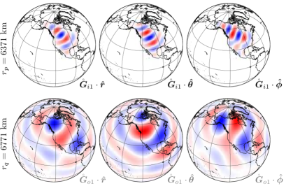
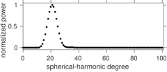
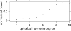
Figure 4: The highest-eigenvalue full-field altitude-cognizant gradient vector Slepian function, internal field $\mathring{\boldsymbol{G}}_{i1}(\boldsymbol{\hat{r}})$ and external field $\mathring{\boldsymbol{G}}_{o1}(\boldsymbol{\hat{r}})$ for region $R=$ North America and ${r_{p}}=6371$ km, ${r_{q}}=6771$ km, ${r_{s}}=6671$ km, $L=100,{L_{o}}=10$. Upper panels: Internal-field part of the function evaluated on the planetary surface defined by ${r_{p}}$. From left to right: radial component, colatitudinal component, longitudinal component. Middle panels: External-field part of the function evaluated at the outer radius ${r_{q}}$. From left to right: radial component, colatitudinal component, longitudinal component. Bottom panels: Power spectra of the internal-field component (bottom left) and external-field component (bottom right).

In Fig. 6 we compare the eigenvalues $\mathbf{\Lambda}$ and $\mathring{\mathbf{\Lambda}}$, obtained from eqs (35) and (55), for this parameter set. The two eigenvalue spectra are similar in character, with few relatively large eigenvalues and most eigenvalues close to zero. The eigenvalue spectra for all the different types of classical Slepian functions presented by Simons et al. (2006), Plattner and Simons (2014), and Plattner and Simons (2015b) typically contained few eigenvalues close to 1 and most eigenvalues close to 0 (the precise numbers depending on the area of the concentration region). Here, even the largest eigenvalues drop below $10^{-5}$. This is because the eigenvalues for the AC-GVSF also include the effects of harmonic continuation: the vector spherical harmonics in eqs (34) and (54) are multiplied by some very small numbers — see eqs (19)–(20).

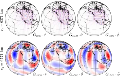
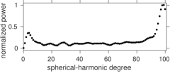
Figure 5: Same layout as Fig. 4 but showing the 500th best-suited internal- and external-field altitude-cognizant gradient vector Slepian function, internal field $\mathring{\boldsymbol{G}}_{i500}(\boldsymbol{\hat{r}})$ and external field $\mathring{\boldsymbol{G}}_{o500}(\boldsymbol{\hat{r}})$ for region $R=$ North America and ${r_{p}}=6371$ km, ${r_{q}}=6771$ km, ${r_{s}}=6671$ km, $L=100,{L_{o}}=10$.

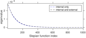
Figure 6: The first 1000 eigenvalues $\lambda_{\alpha}$ for the internal-field only altitude-cognizant gradient vector Slepian functions $G_{\alpha}$, and the first 1000 eigenvalues $\mathring{\lambda}_{\alpha}$ for the internal- and external-field altitude-cognizant gradient vector Slepian functions $\mathring{G}_{\alpha}$.

5.3 Continuous solution by full-field altitude-cognizant gradient vector Slepian functions (AC-GVSF)

Using eqs (54)–(55), we apply the truncated singular value approach to solving eq. (52), as we did in Section 4.3, and obtain

$$\mathring{\mathbf{K}}\begin{pmatrix}\displaystyle\mathrm{v}_{L}^{r_{p}}\\ \\ \displaystyle\mathrm{w}_{L_{o}}^{r_{q}}\end{pmatrix}=\mathring{\mathbf{G}}\mathring{\mathbf{\Lambda}}\mathring{\mathbf{G}}^{\mathrm{T}}\begin{pmatrix}\displaystyle\mathrm{v}_{L}^{r_{p}}\\ \\ \displaystyle\mathrm{w}_{L_{o}}^{r_{q}}\end{pmatrix}=\begin{pmatrix}\displaystyle\mathbf{A}\int_{R}\boldsymbol{\mathcal{E}}_{L}\cdot\boldsymbol{d}\,d\Omega\\ \\ \displaystyle\mathbf{\breve{A}}\int_{R}\boldsymbol{\mathcal{F}}_{L_{o}}\cdot\boldsymbol{d}\,d\Omega\end{pmatrix}.$$ (79)

Since again we only aim to solve eq. (52) for the ${J}$ best-suited full-field AC-GVSF, we use eqs (57) and (78) to write

$$\mathring{\mathbf{G}}_{{J}}\mathring{\mathbf{\Lambda}}_{{J}}\,\mathrm{\tilde{t}}_{J}=\begin{pmatrix}\displaystyle\mathbf{A}\int_{R}\boldsymbol{\mathcal{E}}_{L}\cdot\boldsymbol{d}\,d\Omega\\ \\ \displaystyle\mathbf{\breve{A}}\int_{R}\boldsymbol{\mathcal{F}}_{L_{o}}\cdot\boldsymbol{d}\,d\Omega\end{pmatrix},$$ (80)

with the tilde again distinguishing the truncated solution of eq. (80) from the original statement (79). The matrix $\mathring{\mathbf{G}}_{{J}}$ is as in eq. (58), and $\mathring{\mathbf{\Lambda}}_{{J}}$ is the ${J}$-dimensional version of $\mathring{\mathbf{\Lambda}}$. As previously in eq. (49), a regularized solution of eq. (80) then follows in a form that uses eq. (71),

$$\mathrm{\tilde{t}}_{J}=\mathring{\mathbf{\Lambda}}_{J}^{-1}\int_{R}\mathring{\boldsymbol{\mathcal{G}}}_{\uparrow{J}}\cdot\boldsymbol{d}\,d\Omega.$$ (81)

From the back-projected solution coefficients $\mathring{\mathbf{G}}_{J}\mathrm{\tilde{t}}_{J}$ we can now individually formulate estimates for the internal potential field at radius ${r_{p}}$, and for the external potential field at radius ${r_{q}}$, via eqs (63) and (64),

$$\tilde{V}_{J}({r_{p}}\boldsymbol{\hat{r}}) =\sum_{\alpha=1}^{J}\tilde{t}_{\alpha}\,\mathring{G}_{i\alpha}(\boldsymbol{\hat{r}})=\mathcal{Y}_{L}^{\mathcal{T}}\mathring{\mathbf{G}}_{i{J}}\,\mathrm{\tilde{t}}_{{J}}=\mathring{\mathcal{G}}_{i{J}}^{\mathcal{T}}\,\mathrm{\tilde{t}}_{{J}},$$ (82)

$$\tilde{W}_{J}({r_{q}}\boldsymbol{\hat{r}}) =\sum_{\alpha=1}^{J}\tilde{t}_{\alpha}\,\mathring{G}_{o\alpha}(\boldsymbol{\hat{r}})=\mathcal{Y}^{\mathcal{T}}_{L_{o}}\mathring{\mathbf{G}}_{o{J}}\,\mathrm{\tilde{t}}_{{J}}=\mathring{\mathcal{G}}_{o{J}}^{\mathcal{T}}\,\mathrm{\tilde{t}}_{{J}}.$$ (83)

6 Implementation of the internal-field AC-GVSF method

In Sections 4 and 5 we constructed altitude-aware spatio-spectrally concentrated ‘Slepian’ function bases that can be used as alternatives to vector spherical harmonics to parameterize and solve for potential fields from continuous data. Of course, instrumental data are always collected at a discrete set of points. Thus, in this section we describe how to use the internal-field altitude-cognizant gradient vector Slepian functions (AC-GVSF) of Section 4 to solve for an internal potential field from discrete data at varying satellite altitude. In Section 7 we will use the full-field AC-GVSF of Section 5 to solve for internal- and external potential fields simultaneously.

The continuous problem stated in eqs (30)–(31), after Slepian basis transformation to (47), was solved approximately, analytically, in the truncated form of eq. (49). In the present paper, so far, we have not offered any guidance on how to choose the parameter ${J}$, nor have we shown that solutions of the general type are actually… any good. Reassuringly, Plattner and Simons (2015a) showed that they are, and a statistical analysis confirms this in Section 9. Hence, in this section, we simply furnish the details of a method suitable for practical use.

Let the data be a discrete set of vector-valued measurements obtained at $k$ satellite locations $r_{1}\boldsymbol{\hat{r}}_{1},\ldots,r_{k}\boldsymbol{\hat{r}}_{k}$ in the manner of eq. (30), densely distributed within a subregion $R$ of the unit sphere $\Omega$, at the radial positions ${r_{p}}<r_{i}<{r_{q}}$ clustered about a representative average ${r_{s}}$. We evaluate the vector spherical-harmonics $\boldsymbol{E}_{lm}$ at the data locations $\boldsymbol{\hat{r}}_{1},\ldots,\boldsymbol{\hat{r}}_{k}$ on the unit sphere, multiply them by the corresponding upward-continuation terms $A_{l}(r_{i})$, and collect the results in a $(L+1)^{2}\times 3k$-dimensional matrix ${\boldsymbol{\mathsf{E}}}_{\Uparrow}$. Using the generic index $c$ for $r$, $\theta$ or $\phi$ for the radial, colatitudinal, and longitudinal vector components, and $\mathbf{\hat{c}}$ for $\mathbf{\hat{r}}$, $\hat{\theta}$ or $\hat{\phi}$ for the unit vectors, we assemble the pieces

$$[\boldsymbol{\mathsf{E}}_{\Uparrow lm,i}]_{c}=A_{l}(r_{i})\boldsymbol{E}_{lm}(\boldsymbol{\hat{r}}_{i})\cdot\mathbf{\hat{c}}\quad\mbox{and}\quad[{\boldsymbol{\mathsf{E}}}_{\Uparrow}]_{c}=\begin{pmatrix}[\boldsymbol{\mathsf{E}}_{\Uparrow 00,1}]_{c}&\cdots&[\boldsymbol{\mathsf{E}}_{\Uparrow 00,k}]_{c}\\ \vdots&&\vdots\\ [\boldsymbol{\mathsf{E}}_{\Uparrow LL,1}]_{c}&\cdots&[\boldsymbol{\mathsf{E}}_{\Uparrow LL,k}]_{c}\end{pmatrix}\quad\mbox{into}\quad{\boldsymbol{\mathsf{E}}}_{\Uparrow}=\begin{pmatrix}[{\boldsymbol{\mathsf{E}}}_{\Uparrow}]_{r}&[{\boldsymbol{\mathsf{E}}}_{\Uparrow}]_{\theta}&[{\boldsymbol{\mathsf{E}}}_{\Uparrow}]_{\phi}\end{pmatrix}.$$ (84)

Using the Slepian transformation for the region $R$ and the average satellite altitude ${r_{s}}$, we construct the matrix of ${J}$ internal-field AC-GVSF (compare with eq. 42) evaluated at the actual satellite altitudes $r_{i}$, by multiplying ${\boldsymbol{\mathsf{E}}}_{\Uparrow}$ with the truncated eigenvector matrix $\mathbf{G}_{J}$ of eq. (37),

$${\boldsymbol{\mathsf{G}}}_{\Uparrow J}=\mathbf{G}_{J}^{\mathrm{T}}{\boldsymbol{\mathsf{E}}}_{\Uparrow}.$$ (85)

Broadly speaking, the success of truncation in the Slepian basis as an effective means of regularization owes to the eigenvectors of the ‘normal’ or ‘Gramian’ matrix (34) having relatively easily computable numerical properties and an attractive eigenvalue structure. Thus, rather than discretizing eq. (32) and constructing a truncated-SVD solution for what would amount to a discretized equivalent of eqs (34)–(35), we rely on the data sampling the region of interest $R$ relatively densely, around a relatively stable altitude ${r_{s}}$, and therefore, eq. (85) uses the same, continuously derived, eigenfunctions as in eq. (43), except that they are evaluated at the exact, individual, data altitudes $r_{i}$.

The $3k$-dimensional vector of vector-valued data will be $\mathsf{d}$. Note that we have now introduced a sans-serif ($\mathsf{d},\boldsymbol{\mathsf{E}},\boldsymbol{\mathsf{G}}$) to our lineup of fonts. Using an $\ell_{2}$-norm notation (compare with eq. 31), we restate the inverse problem in the discrete truncated AC-GVSF basis (85) in terms of its unknown expansion coefficients $\hat{s}_{\alpha}$, $\alpha=1,\ldots,{J}$, collecting them in the vector $\hat{\mathrm{s}}_{J}$ (notationally distinct from eqs 46 and 49), as

$$\arg\min_{\hat{\mathrm{s}}_{J}}\left\lVert{\boldsymbol{\mathsf{G}}}_{\Uparrow J}^{\sf T}\hat{\mathrm{s}}_{J}-\mathsf{d}\right\rVert^{2}\quad\mbox{or, equivalently,}\quad\left({\boldsymbol{\mathsf{G}}}_{\Uparrow J}{\boldsymbol{\mathsf{G}}}_{\Uparrow J}^{\sf T}\right)\hat{\mathrm{s}}_{J}={\boldsymbol{\mathsf{G}}}_{\Uparrow J}\mathsf{d}.$$ (86)

Eq. (86) defines a symmetric positive-definite ${J}\times{J}$-dimensional system of equations whose condition number depends on the choice of number of Slepian functions ${J}$ in virtually the same fashion, given our assumptions, as the conditioning of eq. (49) depended on the inverse eigenvalues of the continuous problem. Using the evaluated continuous-problem eigenfunctions is computationally efficient for the inversion, and understanding the behavior of the solutions is promoted through the analysis of their eigenvalues.

However eq. (86) is solved in numerical practice, we advocate following up with the iteratively reweighted residual approach of Farquharson and Oldenburg (1998). We define the $3k$-dimensional vector of residuals $\mathsf{r}$ as

$$\mathsf{r}={\boldsymbol{\mathsf{G}}}_{\Uparrow J}^{\sf T}\,\hat{\mathrm{s}}_{J}-\mathsf{d},$$ (87)

and the $3k\times 3k$-dimensional matrix $\boldsymbol{\mathsf{R}}$ as the diagonal matrix initialized by the identity but in subsequent iterations populated with the absolute values of the entries $\mathsf{r}$ on the diagonal, or a threshold value to avoid division by small numbers for well-fitted data points. Then, we solve the updated linear problem, repeatedly until convergence, by satisfying

$$\left({\boldsymbol{\mathsf{G}}}_{\Uparrow J}\boldsymbol{\mathsf{R}}^{-2}{\boldsymbol{\mathsf{G}}}_{\Uparrow J}^{\sf T}\right)\hat{\mathrm{s}}_{J}={\boldsymbol{\mathsf{G}}}_{\Uparrow J}\boldsymbol{\mathsf{R}}^{-2}\mathsf{d}.$$ (88)

From the $\hat{\mathrm{s}}_{J}$ in eq. (86) or (88) we obtain the estimate $\hat{V}_{J}$ for the potential field on the planetary surface using eq. (39) as in eq. (50),

$$\hat{V}_{J}({r_{p}}\boldsymbol{\hat{r}})=\sum_{\alpha=1}^{J}\hat{s}_{\alpha}G_{\alpha}(\boldsymbol{\hat{r}})=\mathcal{Y}_{L}^{\mathcal{T}}\mathbf{G}_{J}\,\hat{\mathrm{s}}_{{J}}=\mathcal{G}_{J}^{\mathcal{T}}\hat{\mathrm{s}}_{J}.$$ (89)

To evaluate the vector field for the internal potential at a radius within the shell ${r_{p}}\leq r\leq{r_{q}}$, we expand the coefficients $\hat{\mathrm{s}}_{{J}}$ in the Slepian basis evaluated at a different altitude, using eq. (19), and with, as compared to eq. (43), $\boldsymbol{\mathcal{G}}_{\uparrow{J}}(r\boldsymbol{\hat{r}})=\mathbf{G}_{J}^{\mathrm{T}}\mathbf{A}(r)\,\boldsymbol{\mathcal{E}}_{L}(\boldsymbol{\hat{r}})$,

$$\mbox{\boldmath$\nabla$}\hat{V}_{J}(r\boldsymbol{\hat{r}})=\boldsymbol{\mathcal{G}}^{\mathcal{T}}_{\uparrow{J}}(r\boldsymbol{\hat{r}})\,\hat{\mathrm{s}}_{{J}}.$$ (90)

7 Implementation of the full-field AC-GVSF method

In this section we start from data collected in the manner of eq. (51) and use the full-field AC-GVSF of Section 5 to solve for the internal field $\tilde{V}$ on the planetary surface ${r_{p}}$, and an external field $\tilde{W}$ on the outer sphere of radius ${r_{q}}$. Adding to the material developed in Section 6 we now need to build the $[({L_{o}}+1)^{2}-1]\times 3k$-dimensional matrix ${\boldsymbol{\mathsf{F}}}_{\Uparrow}$ of external-field gradient vector spherical harmonics $\boldsymbol{F}_{lm}$ evaluated at the individual data locations $r_{1}\boldsymbol{\hat{r}}_{1},\ldots,r_{k}\boldsymbol{\hat{r}}_{k}$. The matrix entries are defined analogously to eq. (84), namely

$$[\boldsymbol{\mathsf{F}}_{\Uparrow lm,i}]_{c}=\breve{A}_{l}(r_{i})\,\boldsymbol{F}_{lm}(\boldsymbol{\hat{r}}_{i})\cdot\mathbf{\hat{c}},\qquad[{\boldsymbol{\mathsf{F}}}_{\Uparrow}]_{c}=\begin{pmatrix}[\boldsymbol{\mathsf{F}}_{\Uparrow 1\,-1,1}]_{c}&\cdots&[\boldsymbol{\mathsf{F}}_{\Uparrow 1\,-1,k}]_{c}\\ \vdots&&\vdots\\ [\boldsymbol{\mathsf{F}}_{\Uparrow{L_{o}}{L_{o}},1}]_{c}&\cdots&[\boldsymbol{\mathsf{F}}_{\Uparrow{L_{o}}{L_{o}},k}]_{c}\end{pmatrix}\quad\mbox{and}\quad{\boldsymbol{\mathsf{F}}}_{\Uparrow}=\begin{pmatrix}[{\boldsymbol{\mathsf{F}}}_{\Uparrow}]_{r}&[{\boldsymbol{\mathsf{F}}}_{\Uparrow}]_{\theta}&[{\boldsymbol{\mathsf{F}}}_{\Uparrow}]_{\phi}\end{pmatrix}.$$ (91)

Since the truncated full-field AC-GVSF coefficient matrix $\mathring{\mathbf{G}}_{J}$ in eq. (56) contains coefficients pertaining to both internal- and external-field gradient vector spherical harmonics, we can assemble the matrix of ${J}$ full-field altitude cognizant gradient vector Slepian functions evaluated at the varying satellite locations by multiplying the combined matrices ${\boldsymbol{\mathsf{E}}}_{\Uparrow}$ and ${\boldsymbol{\mathsf{F}}}_{\Uparrow}$ with the Slepian coefficient matrix $\mathring{\mathbf{G}}_{J}$,

$$\mathring{\boldsymbol{\mathsf{G}}}_{\Uparrow{J}}=\mathring{\mathbf{G}}_{J}^{\mathrm{T}}\begin{pmatrix}{\boldsymbol{\mathsf{E}}}_{\Uparrow}\\ {\boldsymbol{\mathsf{F}}}_{\Uparrow}\end{pmatrix}.$$ (92)

Compared to eq. (86), the least-squares formulation for the full-field problem in the discrete basis (92) is now in terms of the unknown $\mathrm{\hat{t}}_{{J}}$,

$$\arg\min_{\mathrm{\tilde{t}}_{{J}}}\left\lVert\mathring{\boldsymbol{\mathsf{G}}}_{\Uparrow{J}}^{\sf T}\mathrm{\hat{t}}_{{J}}-\mathsf{d}\right\rVert^{2}\quad\mbox{or, equivalently,}\quad\left(\mathring{\boldsymbol{\mathsf{G}}}_{\Uparrow{J}}\mathring{\boldsymbol{\mathsf{G}}}_{\Uparrow{J}}^{\sf T}\right)\mathrm{\hat{t}}_{J}=\mathring{\boldsymbol{\mathsf{G}}}_{\Uparrow{J}}\mathsf{d}.$$ (93)

As for the purely internal-field solution, we utilize an iteratively reweighted residual approach Farquharson and Oldenburg (1998), with

$$\left(\mathring{\boldsymbol{\mathsf{G}}}_{\Uparrow{J}}\mathring{\boldsymbol{\mathsf{R}}}^{-2}\mathring{\boldsymbol{\mathsf{G}}}_{\Uparrow{J}}^{\sf T}\right)\mathrm{\hat{t}}_{{J}}=\mathring{\boldsymbol{\mathsf{G}}}_{\Uparrow{J}}\mathring{\boldsymbol{\mathsf{R}}}^{-2}\mathsf{d},$$ (94)

and where, in the first iteration, the diagonal weighting matrix $\boldsymbol{\mathsf{R}}$ is the identity and, in later iterations, has on its diagonal the absolute values of $\mathring{\mathsf{r}}$, or a threshold value for small entries of $\mathring{\mathsf{r}}$, where

$$\mathring{\mathsf{r}}=\mathring{\boldsymbol{\mathsf{G}}}_{\Uparrow{J}}^{\sf T}\mathrm{\hat{t}}_{{J}}-\mathsf{d},$$ (95)

the $3k$-dimensional vector of residuals at the individual data locations.

From the obtained coefficient vector $\mathrm{\tilde{t}}_{{J}}$ we construct estimates of the internal potential $\hat{V}_{J}({r_{p}}\boldsymbol{\hat{r}})$ and the external potential $\hat{W}_{J}({r_{q}}\boldsymbol{\hat{r}})$ at ${r_{p}}$ and ${r_{q}}$, respectively, using eqs (61)–(62) as in eqs (82)–(83), which leads to

$$\hat{V}_{J}({r_{p}}\boldsymbol{\hat{r}}) =\sum_{\alpha=1}^{J}\hat{t}_{\alpha}\mathring{G}_{i\alpha}(\boldsymbol{\hat{r}})=\mathcal{Y}_{L}^{\mathcal{T}}\mathring{\mathbf{G}}_{i{J}}\,\mathrm{\hat{t}}_{{J}}=\mathring{\mathcal{G}}_{i{J}}^{\mathcal{T}}\mathrm{\hat{t}}_{{J}},$$ (96)

$$\hat{W}_{J}({r_{q}}\boldsymbol{\hat{r}}) =\sum_{\alpha=1}^{J}\hat{t}_{\alpha}\mathring{G}_{o\alpha}(\boldsymbol{\hat{r}})=\mathcal{Y}^{\mathcal{T}}_{L_{o}}\mathring{\mathbf{G}}_{o{J}}\,\mathrm{\hat{t}}_{{J}}=\mathring{\mathcal{G}}_{o{J}}^{\mathcal{T}}\mathrm{\hat{t}}_{{J}}.$$ (97)

To obtain estimates of the internal and external vector fields at ${r_{p}}<r<{r_{q}}$, we expand $\mathrm{\tilde{t}}_{{J}}$ in the upward-continued internal-field or external-field basis. Using eq. (20) and, instead of eqs (69)–(70), $\mathring{\boldsymbol{\mathcal{G}}}_{i\uparrow{J}}(r\boldsymbol{\hat{r}})=\mathring{\mathbf{G}}^{\mathrm{T}}_{i{J}}\mathbf{A}(r)\,\boldsymbol{\mathcal{E}}_{L}(\boldsymbol{\hat{r}})$ and $\mathring{\boldsymbol{\mathcal{G}}}_{o\uparrow{J}}(r\boldsymbol{\hat{r}})=\mathring{\mathbf{G}}^{\mathrm{T}}_{o{J}}\mathbf{\breve{A}}(r)\,\boldsymbol{\mathcal{F}}_{L_{o}}(\boldsymbol{\hat{r}})$,

$$\mbox{\boldmath$\nabla$}\hat{V}_{J}(r\boldsymbol{\hat{r}}) =\mathring{\boldsymbol{\mathcal{G}}}^{\mathcal{T}}_{i\uparrow{J}}(r\boldsymbol{\hat{r}})\,\mathrm{\hat{t}}_{{J}},$$ (98)

$$\mbox{\boldmath$\nabla$}\hat{W}_{J}(r\boldsymbol{\hat{r}}) =\mathring{\boldsymbol{\mathcal{G}}}^{\mathcal{T}}_{o\uparrow{J}}(r\boldsymbol{\hat{r}})\,\mathrm{\hat{t}}_{{J}},$$ (99)

or indeed, the complete estimate of the full field in eq. (12),

$$\hat{\boldsymbol{B}}_{J}(r\boldsymbol{\hat{r}})=\mathring{\boldsymbol{\mathcal{G}}}^{\mathcal{T}}_{\uparrow{J}}(r\boldsymbol{\hat{r}})\,\mathrm{\hat{t}}_{{J}},$$ (100)

where the equivalent to eq. (71) now takes the form

$$\mathring{\boldsymbol{\mathcal{G}}}_{\uparrow{J}}(r\boldsymbol{\hat{r}})=\begin{pmatrix}\mathring{\mathbf{G}}_{i{J}}^{\mathrm{T}}&\mathring{\mathbf{G}}_{o{J}}^{\mathrm{T}}\end{pmatrix}\begin{pmatrix}\mathbf{A}(r)\,\boldsymbol{\mathcal{E}}_{L}(\boldsymbol{\hat{r}})\\ \mathbf{\breve{A}}(r)\,\boldsymbol{\mathcal{F}}_{L_{o}}(\boldsymbol{\hat{r}})\end{pmatrix}=\mathring{\boldsymbol{\mathcal{G}}}_{i\uparrow{J}}(r\boldsymbol{\hat{r}})+\mathring{\boldsymbol{\mathcal{G}}}_{o\uparrow{J}}(r\boldsymbol{\hat{r}}).$$ (101)

8 Example: Crustal magnetic field reconstruction

We test the internal-field method of Section 6 and the full-field method of Section 7 on a synthetic data set generated as the sum of the internal-field model NGDC-720 V3 Maus (2010), truncated at spherical-harmonic degree $L=100$, and an external field simulated from a flat power spectrum with maximum spherical-harmonic degree ${L_{o}}=10$. We normalize the external-field coefficients such that the resulting field has 10% of the average absolute value of the internal field at the average satellite radial position ${r_{s}}=6671$ km. Such values seem to be within a realistic range, see for example Langel and Estes (1985) and Olsen et al. (2010a). We evaluate both fields at 15000 uniformly distributed data locations within North America at a set of satellite altitudes uniformly distributed between 250 km and 350 km above the planetary radius ${r_{p}}=6371$ km. We add zero-mean uncorrelated Gaussian noise with standard deviation of 1% of the mean absolute value of the combined internal and external fields to the data.

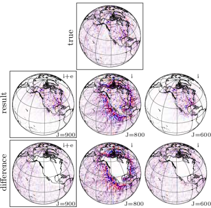
radial field [nT]

Figure 7: Performance of the methods developed in this paper, carried out on a synthetic data set. All panels show the radial component of magnetic fields. For the inversion results, ${J}$ identifies the number of Slepian functions used. Top: the ‘true’ field, composed of internally and externally generated sources, with noise added. Middle left: inversion result using full-field altitude-cognizant gradient vector Slepian functions (AC-GVSF). Middle: inversion result using internal-field AC-GVSF, with ${J}=800$. Middle right: inversion result using internal-field AC-GVSF, with ${J}=600$. Bottom: difference between the true field and the inversion results. The boxed panels are reference cases that reappear in subsequent figures.

To determine the optimal number ${J}_{\mathrm{opt}}$ of Slepian functions we use the procedure described by Plattner and Simons (2015b). We invert for the crustal magnetic field for a series of values ${J}$ of Slepian functions and compare each result to the original field. We select ${J}_{\mathrm{opt}}$ as the number of functions that leads to the smallest mean-squared error within the region $R=$ North America. Such a procedure would not be applicable without knowing the original field. In that case we need to resort to an indirect strategy, as for example the approach described by Plattner and Simons (2015a), or via subsampling methods (e.g. Davison and Hinkley, 1997). For the full-field AC-GVSF method, our best number of Slepian functions was ${J}_{\mathrm{opt}}=900$. For the internal-field AC-GVSF, ${J}_{\mathrm{opt}}=800$, though we note that we achieved a similarly low mean-squared error over North America when ${J}=600$.

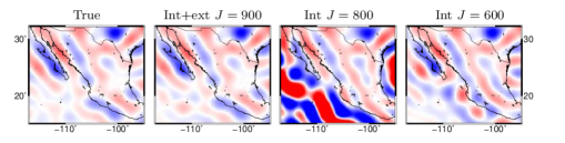
radial field [nT]

Figure 8: Performance of the methods developed in this paper. Close-up over Mexico of the results shown in Fig. 7, identifiable by their labels. While the solutions generally look very similar there are differences, in particular around longitude $-102^{\circ}$ and latitude $20^{\circ}$. A seemingly continuous ‘stripe’ in both internal-field solutions, ${J}=600$ and ${J}=800$, is not continuous in the true field nor in the ‘best’ solution that uses ${J}=900$ full-field altitude-cognizant gradient vector Slepian functions.

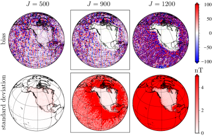
Figure 9: Performance of the methods developed in this paper. Bias and standard deviation of the inversion results for a sequence of $k_{m}=10$ realizations of the data set as shown in Fig. 7, conducted using various ${J}$ full-field altitude-cognizant gradient vector Slepian functions. From these experiments we determined the bias (top row) and the standard deviation (bottom row). Left-hand column: ${J}=500$: significant bias within the North American target region but low variance. Right-hand column: ${J}=1200$: low bias, high variance. Middle column: ${J}_{\mathrm{opt}}=900$: low bias and low variance within the region.

Fig. 7 summarizes the results. We show the radial component of the original NGDC-720 V3 internal field on the planetary surface (top, labeled ‘true’), together with the models resulting from our full-field approach using ${J}_{\mathrm{opt}}=900$ (middle, labeled ‘i+e’), and the result from the internal-field approach using ${J}_{\mathrm{opt}}=800$ and ${J}=600$ (middle, labeled ‘i’). The bottom row shows the differences between the true model and the inversion results. The results for the full-field method for ${J}_{\mathrm{opt}}=900$ and for the internal-field method when ${J}=600$ show little model strength outside of the North American region, whereas the result from the internal-field method when ${J}=800$ shows significant ringing off the coast of North America. This ringing results from the increased model variance caused by functions that have significant energy outside North America, where they are unconstrained by data. For larger numbers ${J}$ of Slepian functions this variance will also affect the model within the region of North America. In Fig. 7 we framed the original model, the panels representing our ‘optimal’ solution, and the difference between the two. The panels with the original field and the best model will reappear for comparison later.

The full-field AC-GVSF solution shown Fig. 7 (middle left) faithfully represents the original model (top), a finding that is substantiated by their difference (bottom left). At first glance, the purely internal-field AC-GVSF solutions (panels labeled ‘i’) also do appear representative within North America. Upon closer inspection, shown in Fig. 8, both ${J}=800$ and ${J}=600$ internal-field solutions contain similar artifacts which may lead to misinterpretation, in particular since they persist for different numbers of Slepian functions, and because they are of smaller length scale than supported by the bandwidth ${L_{o}}=10$ of the external field for which we did not account in those inversions.

When selecting the optimal number ${J}_{\mathrm{opt}}$ of Slepian functions we aim to minimize the mean-squared error of the resulting model. With increasing ${J}$ the model bias decreases, whereas its variance increases. While we postpone a more formal statistical analysis for the internal-field method to Section 9, and for the full-field method to Section 10, this behavior can be understood on the basis of elementary considerations Simons and Dahlen (2006); Plattner and Simons (2015b); Freeden et al. (2016). Up to a point, modeling using more Slepian functions implies that less ‘signal’ is being missed over the target region, but also that more ‘noise’ is being captured. We calculate the spatial manifestation of the model bias (the difference between the known truth and the average estimated model), and its variance (the average of the squared difference between the estimated models and their average) in our numerical examples for three different numbers ${J}$ of Slepian functions, based on individual inversions for each of $k_{m}=10$ realizations of our synthetic data set, which differ only in the realizations of the added noise. Bias and standard deviation for the full-field approach are shown in Fig. 9, for the cases ${J}=500$ (too few Slepian functions), ${J}_{\mathrm{opt}}=900$ (our selected solution), and ${J}=1200$ (too many Slepian functions). The top row of Fig. 9 shows the bias, the bottom row shows the corresponding standard deviation.

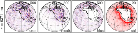
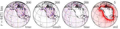
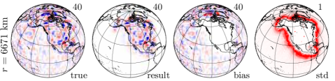
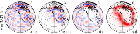
Figure 10: The effect of upward continuation of the estimated model. The known model (‘true’), internal-field results of a full-field inversion (‘result’), difference between the true model and the average of the inversion results (‘bias’), and standard deviation of the model results (‘std’), over $k_{m}=10$ inversions. All models are evaluated on the planetary surface (first row), between the planetary surface and the satellite (at 100 km altitude, second row), at average satellite altitude 300 km (third row) and at 1000 km above the planet (fourth row). The $\pm$limits of the color bar (where we mark them collectively as ‘$\pm$lim’) are indicated by the numbers in the top right of each panel.

With increasing number ${J}$ of functions the bias decreases, but the standard deviation increases. Selecting too few (${J}=500$) functions (left-hand column), a low standard deviation is achieved at the expense of a large bias within the North American target region $R$. If, on the other hand, we use too many (${J}=1200$) functions (right-hand column), a small bias within the region comes at the expense of a large standard deviation. Only the right number (${J}_{\mathrm{opt}}=900$) of functions (middle column) has both low bias and a small standard deviation within the region. The framed panels correspond to the reference solutions shown in Fig. 7.

To illustrate the effects of upward continuing the estimated internal field, as described by eq. (98), Fig. 10 shows the original model (leftmost column), the full-field inversion result (second from left), bias (third from left), and standard deviation (rightmost column) for different evaluation altitudes. The framed panels in the top row show the original field, resulting model, bias, and variance on the planetary surface, exactly as they appeared in Figs. 7 and 9. The second through fourth rows of Fig. 10 show the original field and results reevaluated at different altitudes, together with their bias and standard deviation. A single color bar serves all panels, with the color limits listed in the upper right corner of each panel. For radial position $r=6471$ km, $100$ km altitude, and for radial position $r=6671$ km, corresponding to the average satellite altitude of the simulated data, both bias and standard deviation are low within the North American target region.

Upward continuation beyond the satellite altitude, up to 1000 km above the planetary surface, inflates the standard deviation within the region, where it reaches up to 3% of the maximum values of the field. Outside of the target region the model is not well resolved. This leads to a strong dependence on noise which is greatest close to the region where the selected Slepian functions still have relatively high energy but are not well constrained by the data. Further away from the region, the Slepian functions have less power, and the resulting model power and, with it, the standard deviation, are weaker.

9 Analysis of the internal-field AC-GVSF method

In the previous sections we discussed how our methods work, while the results of Plattner and Simons (2015a) showed that, indeed, they do work. In this section, we show why. To this end we introduce some more notation. We take inspiration from eq. (43) to define the vectors of (truncated) downward-continued AC-GVSF, namely

$$\boldsymbol{\mathcal{G}}_{\downarrow}=\mathbf{G}^{\mathrm{T}}\mathbf{A}^{-1}\boldsymbol{\mathcal{E}}_{L}\quad\mbox{and}\quad\boldsymbol{\mathcal{G}}_{\downarrow{J}}=\mathbf{G}_{J}^{\mathrm{T}}\mathbf{A}^{-1}\boldsymbol{\mathcal{E}}_{L},$$ (102)

as well as the complement $\boldsymbol{\mathcal{G}}_{\uparrow>{J}}$, the vector with the remaining $(L+1)^{2}-{J}$ altitude-cognizant gradient vector Slepian functions. With these expressions we state the important relationships

$$\boldsymbol{\mathcal{G}}_{\uparrow}^{\mathcal{T}}\boldsymbol{\mathcal{G}}_{\downarrow}=\boldsymbol{\mathcal{G}}_{\downarrow}^{\mathcal{T}}\boldsymbol{\mathcal{G}}_{\uparrow}=\boldsymbol{\mathcal{E}}_{L}^{\mathcal{T}}\mathbf{A}^{-\mathrm{T}}\mathbf{G}\mathbf{G}^{\mathrm{T}}\mathbf{A}\,\boldsymbol{\mathcal{E}}_{L}=\boldsymbol{\mathcal{E}}_{L}^{\mathcal{T}}\boldsymbol{\mathcal{E}}_{L}.$$ (103)

With the above we can now rewrite the infinitely wideband eq. (17), at satellite altitude, in the following equivalent forms,

$$\mbox{\boldmath$\nabla$}V =\boldsymbol{\mathcal{E}}_{L}^{\mathcal{T}}\int_{\Omega}\boldsymbol{\mathcal{E}}_{L}\cdot\mbox{\boldmath$\nabla$}V\,d\Omega+\boldsymbol{\mathcal{E}}_{>L}^{\mathcal{T}}\int_{\Omega}\boldsymbol{\mathcal{E}}_{>L}\cdot\mbox{\boldmath$\nabla$}V\,d\Omega$$ (104)

$$=\boldsymbol{\mathcal{G}}^{\mathcal{T}}_{\uparrow}\int_{\Omega}\boldsymbol{\mathcal{G}}_{\downarrow}\cdot\mbox{\boldmath$\nabla$}V\,d\Omega+\boldsymbol{\mathcal{E}}_{>L}^{\mathcal{T}}\int_{\Omega}\boldsymbol{\mathcal{E}}_{>L}\cdot\mbox{\boldmath$\nabla$}V\,d\Omega$$ (105)

$$=\boldsymbol{\mathcal{E}}_{L}^{\mathcal{T}}\mathbf{A}\mathrm{v}_{L}^{r_{p}}+\boldsymbol{\mathcal{E}}_{>L}^{\mathcal{T}}\int_{\Omega}\boldsymbol{\mathcal{E}}_{>L}\cdot\mbox{\boldmath$\nabla$}V\,d\Omega.$$ (106)

9.1 Relationship to classical spherical Slepian functions

The optimization problem in eq. (31) led to the diagonalization of the matrix $\mathbf{K}$ in eq. (34) via eq. (35). The coefficients $\mathbf{G}$ in eq. (37) also solve an energy concentration maximization problem in the space of bandlimited upward-continued vector spherical-harmonic functions, as we can see through the formalism in eqs (40) and (43), given the equivalency

$$\lambda=\frac{\mathrm{g}^{\mathrm{T}}\mathbf{K}\,\mathrm{g}}{\mathrm{g}^{\mathrm{T}}\mathrm{g}}=\frac{\displaystyle\int_{R}\left(\mathrm{g}^{\mathrm{T}}\mathbf{A}\,\boldsymbol{\mathcal{E}}_{L}\right)\cdot\left(\boldsymbol{\mathcal{E}}_{L}^{\mathcal{T}}\mathbf{A}^{\mathrm{T}}\mathrm{g}\right)d\Omega}{\displaystyle\int_{\Omega}\left(\mathrm{g}^{\mathrm{T}}\mathcal{Y}_{L}\right)\left(\mathcal{Y}_{L}^{\mathcal{T}}\mathrm{g}\right)d\Omega}=\frac{\displaystyle\int_{R}\boldsymbol{G}_{\uparrow}^{2}\,d\Omega}{\displaystyle\int_{\Omega}G^{2}\,d\Omega}=\mathrm{maximum}.$$ (107)

Appearing without the factor $\mathbf{A}$ of eq. (21) in the numerator, eq. (107) is a ‘classical’ (gradient-)vector spherical-harmonic concentration problem in the style of Maniar and Mitra (2005), Plattner and Simons (2014, 2015b), and Jahn and Bokor (2014), much as these authors generalized the ‘classical’ scalar problem of Albertella et al. (1999), Simons et al. (2006), Simons and Dahlen (2006), and others — see also Eshagh (2009). Among all bandlimited upward-continued gradient-vector functions that are linear combinations of the basis set $\mathbf{A}\,\boldsymbol{\mathcal{E}}_{L}$, the first altitude-cognizant gradient vector Slepian function, $\boldsymbol{G}_{\uparrow 1}$, is the best-concentrated in the sense of (107). The concentration factor $\lambda_{1}$ is the first eigenvalue associated with the diagonalization problem (35). The second-best concentrated AC-GVSF, $\boldsymbol{G}_{\uparrow 2}$, and its corresponding $\lambda_{2}$, is the next best function in the sense (107) that is orthogonal to $\boldsymbol{G}_{\uparrow 1}$, and so on.

Evaluated at satellite altitude, the internal-field AC-GVSF $\boldsymbol{\mathcal{G}}_{\uparrow\alpha}$ of eq. (43) are mutually orthogonal over the region $R$ but not over the sphere $\Omega$. On the planetary surface, the corresponding scalar functions $\mathcal{G}_{\alpha}$ of eq. (40) are orthogonal over the entire sphere but not over $R$. With $\mathbf{\Lambda}$ the eigenvalue matrix as in eq. (35) and $\mathbf{I}$ the identity, it is straightforward to verify that

$$\int_{R}\boldsymbol{\mathcal{G}}_{\uparrow}\cdot\boldsymbol{\mathcal{G}}_{\uparrow}^{\mathcal{T}}\,d\Omega =\mathbf{\Lambda}\quad\mbox{and}\quad\int_{\Omega}\boldsymbol{\mathcal{G}}_{\uparrow}\cdot\boldsymbol{\mathcal{G}}_{\uparrow}^{\mathcal{T}}\,d\Omega=\mathbf{G}^{\mathrm{T}}\mathbf{A}\mathbf{A}^{\mathrm{T}}\mathbf{G},$$ (108)

$$\int_{\Omega}\mathcal{G}\,\mathcal{G}^{\mathcal{T}}\,d\Omega =\mathbf{I},\quad\mbox{and}\quad\int_{R}\mathcal{G}\,\mathcal{G}^{\mathcal{T}}\,d\Omega=\mathbf{G}^{\mathrm{T}}\left(\int_{R}\mathcal{Y}_{L}\mathcal{Y}_{L}^{\mathcal{T}}d\Omega\right)\mathbf{G}.$$ (109)

For truncated Slepian bases we also have the corresponding projective relationships

$$\int_{R}\boldsymbol{\mathcal{G}}_{\uparrow{J}}\cdot\boldsymbol{\mathcal{G}}_{\uparrow}^{\mathcal{T}}\,d\Omega=\begin{pmatrix}\mathbf{\Lambda}_{{J}}&\mathbf{0}\end{pmatrix}\quad\text{ and }\quad\int_{\Omega}\mathcal{G}_{{J}}\,\mathcal{G}^{\mathcal{T}}\,d\Omega=\begin{pmatrix}\mathbf{I}_{{J}}&\mathbf{0}\end{pmatrix}.$$ (110)

The ‘localization’ matrix $\int_{R}\mathcal{Y}_{L}\mathcal{Y}_{L}^{\mathcal{T}}d\Omega$ in eq. (109) is one that appears in the construction of the classical scalar Slepian functions Simons et al. (2006); Simons and Dahlen (2006). Its eigenvectors lead to spherical functions that are orthogonal over the region $R$, but also over the entire sphere $\Omega$. Incorporating the upward-continuation into the construction of the Slepian functions has induced a loss of orthogonality over the region $R$ on the planetary surface (eq. 109) — but we gained orthogonality within $R$ at satellite altitude (eq. 108).

9.2 Spatially restricted, spectrally concentrated internal-field Slepian functions

As shown by Simons et al. (2006), bandlimited spatially concentrated Slepian functions have broadband relatives that are spacelimited but spectrally concentrated. As shown by Simons and Dahlen (2006) such functions play an important role in the analysis of inversion problems like the one that we are treating in this paper. Spacelimited vector Slepian functions were introduced by Plattner and Simons (2014), and spacelimited gradient-vector Slepian functions by Plattner and Simons (2015b). As to the spacelimited altitude-cognizant-gradient vector Slepian functions that we will be needing here, we define the vector with the the first ${J}$ of the $\boldsymbol{H}_{\uparrow\alpha,>L}=\mathrm{h}^{\mathrm{T}}_{\uparrow\alpha,>L}\boldsymbol{\mathcal{E}}_{>L}$,

$$\boldsymbol{\mathcal{H}}_{\uparrow J,>L}=\begin{pmatrix}\boldsymbol{H}_{\uparrow 1,>L}&\cdots&\boldsymbol{H}_{\uparrow\alpha,>L}&\cdots&\boldsymbol{H}_{\uparrow{J},>L}\end{pmatrix}^{T}=\left(\int_{R}\boldsymbol{\mathcal{G}}_{\uparrow{J}}\cdot\boldsymbol{\mathcal{E}}_{>L}^{\mathcal{T}}\,d\Omega\right)\boldsymbol{\mathcal{E}}_{>L},$$ (111)

where the infinite-dimensional vector $\mathrm{h}_{\uparrow\alpha}$ that contains the expansion coefficients in the full basis set $\boldsymbol{E}_{lm}$, $0<l<\infty$, $-l<m<l$, of the bandlimited AC-GVSF $\boldsymbol{G}_{\uparrow\alpha}$ after spatial truncation to the region $R$, and the infinite vector $\mathrm{h}_{\uparrow\alpha,>L}$ containing only those components at the degrees $l>L$, respectively, for each $\alpha=1,\ldots,(L+1)^{2}$, are, from eq. (43),

$$\mathrm{h}_{\uparrow\alpha}=\int_{R}\boldsymbol{\mathcal{E}}\cdot\boldsymbol{G}_{\uparrow\alpha}\,d\Omega=\left(\int_{R}\boldsymbol{\mathcal{E}}\cdot\boldsymbol{\mathcal{E}}_{L}^{\mathcal{T}}d\Omega\right)\mathbf{A}^{\mathrm{T}}\mathrm{g}_{\alpha}\quad\mbox{and}\quad\mathrm{h}_{\uparrow\alpha,>L}=\int_{R}\boldsymbol{\mathcal{E}}_{>L}\cdot\boldsymbol{G}_{\uparrow\alpha}\,d\Omega=\left(\int_{R}\boldsymbol{\mathcal{E}}_{>L}\cdot\boldsymbol{\mathcal{E}}_{L}^{\mathcal{T}}d\Omega\right)\mathbf{A}^{\mathrm{T}}\mathrm{g}_{\alpha}.$$ (112)

The coefficient sets $\mathrm{h}_{\uparrow\alpha}$ and $\mathrm{h}_{\uparrow\alpha,>L}$ relate to the set of coefficients $\mathbf{A}^{\mathrm{T}}\mathrm{g}_{\alpha}$ of the bandlimited functions $\boldsymbol{G}_{\uparrow\alpha}$ via broadband extensions of the localization matrix $\int_{R}\boldsymbol{\mathcal{E}}_{L}\cdot\boldsymbol{\mathcal{E}}_{L}^{\mathcal{T}}d\Omega$ in eq. (32), in the same manner as did their equivalents in the scalar and vector cases discussed above.

9.3 Statistical analysis of the internal-field method

We now return to the issue we mentioned in Section 3, namely, how spherical-harmonic model bandlimitation affects the estimate made from data that have, per eq. (17), in principle, infinite bandwidth. What are we missing? And, what is the effect of truncation of the Slepian basis?

We begin by rewriting the bandlimited portion of the internal potential (4) in terms of the internal-field altitude-cognizant scalar Slepian functions of eq. (40), which, owing to their orthogonality (109), remain a complete basis for bandlimited functions on the sphere, see eqs (44)–(46). To the Slepian expansion we add the broadband components,

$$V({r_{p}}\boldsymbol{\hat{r}})=\mathcal{G}_{J}^{\mathcal{T}}\int_{\Omega}\mathcal{G}_{J}V({r_{p}}\boldsymbol{\hat{r}})\,d\Omega+\mathcal{G}_{>{J}}^{\mathcal{T}}\int_{\Omega}\mathcal{G}_{>{J}}V({r_{p}}\boldsymbol{\hat{r}})\,d\Omega+\mathcal{Y}_{>L}^{\mathcal{T}}\int_{\Omega}\mathcal{Y}_{>L}V({r_{p}}\boldsymbol{\hat{r}})\,d\Omega.$$ (113)

Next, we rewrite eq. (30) in terms of the AC-GVSF with the help of eq. (105). The continuous data representation is then given by

$$\boldsymbol{d}=\boldsymbol{\mathcal{G}}_{\uparrow}^{\mathcal{T}}\int_{\Omega}\boldsymbol{\mathcal{G}}_{\downarrow}\cdot\mbox{\boldmath$\nabla$}V\,d\Omega+\boldsymbol{\mathcal{E}}_{>L}^{\mathcal{T}}\int_{\Omega}\boldsymbol{\mathcal{E}}_{>L}\cdot\mbox{\boldmath$\nabla$}V\,d\Omega+\boldsymbol{n}.$$ (114)

Finally, we return to the form of the bandlimited truncated internal-field AC-GVSF estimator in eqs (49)–(50), restated as

$$\tilde{V}_{J}({r_{p}}\boldsymbol{\hat{r}})=\mathcal{G}_{J}^{\mathcal{T}}\mathbf{\Lambda}^{-1}_{J}\int_{R}\boldsymbol{\mathcal{G}}_{\uparrow{J}}\cdot\boldsymbol{d}\,d\Omega.$$ (115)

As noted before, the estimator (115) is the one used by Plattner and Simons (2015a), which is rather radically different from its counterpart discussed by Plattner and Simons (2015b). However, and issues of notation cast aside, the derivations below retain the full character of the material presented by Plattner and Simons (2015b) — or, mutatis mutandis, by Simons and Dahlen (2006) — hence our abridged treatment here.

Inserting eq. (114) into eq. (115), we use eqs (110) and (111), and further using eqs (106), (102), the orthonormality (11) of the $\boldsymbol{\mathcal{E}}$, and, at last, eqs (44)–(46), we obtain the expression

$$\tilde{V}_{J}({r_{p}}\boldsymbol{\hat{r}})=\mathcal{G}_{J}^{\mathcal{T}}\int_{\Omega}\mathcal{G}_{J}V({r_{p}}\boldsymbol{\hat{r}})\,d\Omega+\mathcal{G}_{J}^{\mathcal{T}}\mathbf{\Lambda}^{-1}_{J}\left(\int_{\Omega}\boldsymbol{\mathcal{H}}_{\uparrow J,>L}\cdot\mbox{\boldmath$\nabla$}V\,d\Omega+\int_{R}\boldsymbol{\mathcal{G}}_{\uparrow{J}}\cdot\boldsymbol{n}\,d\Omega\right).$$ (116)

Spherical-harmonic bandlimitation, Slepian-function truncation, and noise are the three ingredients necessary to understand the quality of our estimates. A direct comparison between the estimate in eq. (116) and the unknown truth in eq. (113) reveals that the bandlimited estimate $\tilde{V}$ of the internal potential field $V$ does not only depend on the bandlimited part of the true but also on its broadband portion, and the noise. Bandlimitation introduces a direct bias term, whether the estimate uses a truncated Slepian basis or not. The latter two terms in eq. (116) are amplified by the inverse eigenvalues, which typically become large for increasing ${J}$, which is the primary reason for truncating the Slepian expansions. The more Slepian functions we use to estimate the internal potential field, the more leakage contributions we pick up from the neglected broadband components and from the noise. On the other hand, if we use too few Slepian functions, then we cannot solve for enough details of the bandlimited internal field.

If we now make the defensible assumptions that the noise term has zero mean, and that the noise is uncorrelated with the signal, we can obtain palatable expressions for the bias, variance, and mean-squared error of our estimates in terms of the power-spectral densities of both signal and noise. Again, we follow the recipes outlined by Simons and Dahlen (2006) or Plattner and Simons (2015b), with the modifications appropriate to our case at hand. The estimation bias, the difference between the expected value of the estimator (116) and the truth (113), is

$$b=-\mathcal{G}_{>{J}}^{\mathcal{T}}\int_{\Omega}\mathcal{G}_{>{J}}V({r_{p}}\boldsymbol{\hat{r}})\,d\Omega-\mathcal{Y}_{>L}^{\mathcal{T}}\int_{\Omega}\mathcal{Y}_{>L}V({r_{p}}\boldsymbol{\hat{r}})\,d\Omega+\mathcal{G}_{J}^{\mathcal{T}}\mathbf{\Lambda}^{-1}_{J}\int_{\Omega}\boldsymbol{\mathcal{H}}_{\uparrow J,>L}\cdot\mbox{\boldmath$\nabla$}V\,d\Omega.$$ (117)

It is clear from eq. (117) that ‘bias’ is caused by ‘missing’ and ‘mismapped’ signal, from the combination of spherical-harmonic bandlimitation and Slepian truncation. A key feature of the Slepian function apparatus, however, is that because the AC-GVSF are spatially concentrated within the target region $R$, with the concentration measured by the usually rapidly diminishing ranked eigenvalues, the bias from neglecting low-ranked eigenfunctions will mostly affect the regions that are not of interest or where no data were collected. Certainly, care should be taken to define the optimal truncation level ${J}_{\mathrm{opt}}$, but in Section 8 we outlined a procedure precisely for doing so.

To avoid complicating matters from now on, we drop broadband terms (the second term in eq. 116, and the last two terms in eq. 117), as without a priori modeling of what we truly do not know: the signal at the unmodeled spherical-harmonic degrees, we are in no position to remediate the broadband bias nor its leakage into the bandlimited estimate. We now consider both the true signal and the noise to be realizations of a time-independent random process that can be characterized by a power-spectral density, or, equivalently, a certain covariance function, in the scalar and vector forms

$$\mathscr{V}({r_{p}}\boldsymbol{\hat{r}},{r_{p}}\boldsymbol{\hat{r}}^{\prime}) =\left\langle V({r_{p}}\boldsymbol{\hat{r}})\,V({r_{p}}\boldsymbol{\hat{r}}^{\prime})\right\rangle,$$ (118)

$$\mathbf{\mathcal{N}}({r_{s}}\boldsymbol{\hat{r}},{r_{s}}\boldsymbol{\hat{r}}^{\prime}) =\left\langle\boldsymbol{n}({r_{s}}\boldsymbol{\hat{r}})\cdot\boldsymbol{n}({r_{s}}\boldsymbol{\hat{r}}^{\prime})\right\rangle.$$ (119)

Upon doing so, the mean-squared estimation error will be given by the expression

$$\mathrm{mse}=\mathcal{G}_{J}^{\mathcal{T}}\mathbf{\Lambda}^{-1}_{J}\left(\int_{R}\boldsymbol{\mathcal{G}}_{\uparrow{J}}\cdot\mathbf{\mathcal{N}}({r_{s}}\boldsymbol{\hat{r}},{r_{s}}\boldsymbol{\hat{r}}^{\prime})\cdot\boldsymbol{\mathcal{G}}^{\mathcal{T}}_{\uparrow{J}}\,d\Omega\right)\mathbf{\Lambda}^{-1}_{J}\mathcal{G}_{J}+\mathcal{G}_{>{J}}^{\mathcal{T}}\left(\int_{\Omega}\int_{\Omega}\mathcal{G}_{>{J}}\mathscr{V}({r_{p}}\boldsymbol{\hat{r}},{r_{p}}\boldsymbol{\hat{r}}^{\prime})\,\mathcal{G}_{>{J}}^{\mathcal{T}}\,d\Omega\,d\Omega^{\prime}\right)\mathcal{G}_{>{J}},$$ (120)

where the first term is the estimation variance, readily computed from the difference between the expectation of the square of eq. (116) and its squared expectation, and the second the expected value of the squared estimation bias in eq. (117), see Cox and Hinkley (1974).

It is a most welcome feature of the Slepian framework that truncation of the basis neatly separates the effects of variance and bias, by projection onto different basis functions altogether. But of course it remains a feature common to all inverse problems that diminishing variance comes at the price of increasing bias, and that solutions that minimize the mean-squared estimation errors are accessible only after experimentation and iteration, as determined by the signal-to-noise ratio of what, ultimately, should turn out to be signal, and what, noise. Disregarding the ultimate complexity of what, practically, needs to be achieved to perform statistically efficient internal-field estimation, eq. (120) shows the ‘knobs’ of the system: a region $R$, a bandwidth $L$, an accompanying satellite-altitude-cognizant Slepian basis that is driving the mean-squared error through its eigenvalue structure $\mathbf{\Lambda}$, and a truncation level ${J}$ that remains to be judiciously chosen.

9.4 Case study I: Bandlimited and spectrally flat signal and noise

Under the admittedly unrealistic if not mathematically impossible scenario where both the signal and the noise should be bandlimited (to the same degree $L$ as the Slepian functions used) and ‘white’ (uncorrelated between any two different space points), with the signal and the noise completely uncorrelated, and with signal power $\mathscr{V}$ and noise power $\mathbf{\mathcal{N}}$, respectively, the expression for the mean-squared error would take a simple form derived from the identities in eq. (108), namely

$$\mathrm{mse}=\mathbf{\mathcal{N}}\,\mathcal{G}_{J}^{\mathcal{T}}\mathbf{\Lambda}^{-1}_{J}\mathcal{G}_{J}+\mathscr{V}\,\mathcal{G}_{>{J}}^{\mathcal{T}}\,\mathcal{G}_{>{J}}.$$ (121)

Eq. (121) is decidedly more palatable when contrasted with the equivalent result (174) of Plattner and Simons (2015b), and thus illustrates the benefits of using altitude-cognizant functions as advocated here. Moreover, we find again eq. (146) from Simons and Dahlen (2006), where it only applied to the zero-altitude case.

The mean-squared error (121) is a function of all of space $\Omega$. To obtain the relative mean-squared error over the target region $R$ we calculate its integral over the region and normalize it by the integral over $R$ of the signal power $\mathscr{V}$, for an example similar to the one described in Section 8.

We set $L=100,{r_{p}}=6371$ km, ${r_{s}}=6671$ km, and $R=$ North America. As per eqs (118)–(119) the signal power $\mathscr{V}=\mathscr{V}({r_{p}})$ is given on the planetary surface, while the noise power $\mathbf{\mathcal{N}}=\mathbf{\mathcal{N}}({r_{s}})$ is at satellite altitude. To calculate the relative mean-squared error for a realistic signal-to-noise level, we need to calculate the signal power on the planetary surface, $\mathscr{V}({r_{p}})$, as a function of that at satellite altitude, $\mathscr{V}({r_{s}})$. Because the signal is white on the surface we distribute the power evenly over the degrees such that each degree contributes $\mathscr{V}({r_{p}})/(L+1)$. We then upward-continue to the satellite altitude by multiplying the values at each degree power by the corresponding factor $A_{lm,l^{\prime}m^{\prime}}^{2}$ in eq. (19), and obtain the signal power at satellite altitude by summing those to obtain $\mathscr{V}({r_{s}})$. For the values for $L$, ${r_{s}}$, and ${r_{p}}$ that we chose, we obtain $\mathscr{V}({r_{p}})\approx 1.1\times 10^{6}\,\mathscr{V}({r_{s}})$. Fig. 11 shows the region-average relative mean-squared error as it depends on the number ${J}$ of internal-field AC-GVSF used, together with the relative squared bias and variance. In this example we set $\mathscr{V}({r_{s}})=1$ and $\mathbf{\mathcal{N}}({r_{s}})=0.01$. The optimal number of Slepian functions ${J}_{\mathrm{opt}}=556$, with a relative mean-squared error of 0.1.

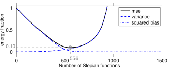
Figure 11: Statistical performance of the truncated Slepian-function solution to the internal-field inversion problem, as computed via eq. (121). Mean-squared error and its constituents, estimation variance and squared bias, all relative to the untruncated values. The optimal number of Slepian functions ${J}_{\mathrm{opt}}=556$ and the corresponding relative mean-squared error (0.1).

10 Analysis of the full-field AC-GVSF method

To understand the effect of bandlimitation and Slepian truncation on the full-field solution, we begin by defining the vectors of (truncated) downward-continued AC-GVSF inspired by eqs (69)–(70), namely

$$\mathring{\boldsymbol{\mathcal{G}}}_{i\downarrow} =\mathring{\mathbf{G}}_{i}^{\mathrm{T}}\mathbf{A}^{-1}\boldsymbol{\mathcal{E}}_{L}\quad\mbox{and}\quad\mathring{\boldsymbol{\mathcal{G}}}_{i\downarrow{J}}=\mathring{\mathbf{G}}_{i{J}}^{\mathrm{T}}\,\mathbf{A}^{-1}\boldsymbol{\mathcal{E}}_{L},$$ (122)

$$\mathring{\boldsymbol{\mathcal{G}}}_{o\downarrow} =\mathring{\mathbf{G}}_{o}^{\mathrm{T}}\mathbf{\breve{A}}^{-1}\boldsymbol{\mathcal{F}}_{L_{o}}\quad\mbox{and}\quad\mathring{\boldsymbol{\mathcal{G}}}_{o\downarrow{J}}=\mathring{\mathbf{G}}_{o{J}}^{\mathrm{T}}\,\mathbf{\breve{A}}^{-1}\boldsymbol{\mathcal{F}}_{L_{o}},$$ (123)

for $1\leq{J}\leq(L+1)^{2}+({L_{o}}+1)^{2}-1$, and their complements, $\mathring{\boldsymbol{\mathcal{G}}}_{i\downarrow>{J}}$ and $\mathring{\boldsymbol{\mathcal{G}}}_{o\downarrow>{J}}$. From the above definitions and together with eq. (71) and eq. (60), we obtain relationships similar to the ones we have for the purely internal-field AC-GVSF in eq. (103),

$$\mathring{\boldsymbol{\mathcal{G}}}_{\uparrow}^{\mathcal{T}}\mathring{\boldsymbol{\mathcal{G}}}_{i\downarrow} =\mathring{\boldsymbol{\mathcal{G}}}_{i\uparrow}^{\mathcal{T}}\mathring{\boldsymbol{\mathcal{G}}}_{i\downarrow}=\mathring{\boldsymbol{\mathcal{G}}}_{i\downarrow}^{\mathcal{T}}\mathring{\boldsymbol{\mathcal{G}}}_{i\uparrow}=\boldsymbol{\mathcal{E}}_{L}^{\mathcal{T}}\mathbf{A}^{-\mathrm{T}}\mathring{\mathbf{G}}_{i}\mathring{\mathbf{G}}_{i}^{\mathrm{T}}\mathbf{A}\,\boldsymbol{\mathcal{E}}_{L}=\boldsymbol{\mathcal{E}}_{L}^{\mathcal{T}}\boldsymbol{\mathcal{E}}_{L},$$ (124)

$$\mathring{\boldsymbol{\mathcal{G}}}_{\uparrow}^{\mathcal{T}}\mathring{\boldsymbol{\mathcal{G}}}_{o\downarrow} =\mathring{\boldsymbol{\mathcal{G}}}_{o\uparrow}^{\mathcal{T}}\mathring{\boldsymbol{\mathcal{G}}}_{o\downarrow}=\mathring{\boldsymbol{\mathcal{G}}}_{o\downarrow}^{\mathcal{T}}\mathring{\boldsymbol{\mathcal{G}}}_{o\uparrow}=\boldsymbol{\mathcal{F}}_{L_{o}}^{\mathcal{T}}\mathbf{\breve{A}}^{-\mathrm{T}}\mathring{\mathbf{G}}_{o}\mathring{\mathbf{G}}_{o}^{\mathrm{T}}\mathbf{\breve{A}}\,\boldsymbol{\mathcal{F}}_{L_{o}}=\boldsymbol{\mathcal{F}}_{L_{o}}^{\mathcal{T}}\boldsymbol{\mathcal{F}}_{L_{o}}.$$ (125)

With these, we rewrite the wideband eqs (17)–(18) in the following equivalent forms,

$$\mbox{\boldmath$\nabla$}V =\boldsymbol{\mathcal{G}}^{\mathcal{T}}_{i\uparrow}\int_{\Omega}\boldsymbol{\mathcal{G}}_{i\downarrow}\cdot\mbox{\boldmath$\nabla$}V\,d\Omega+\boldsymbol{\mathcal{E}}_{>L}^{\mathcal{T}}\int_{\Omega}\boldsymbol{\mathcal{E}}_{>L}\cdot\mbox{\boldmath$\nabla$}V\,d\Omega$$ (126)

$$=\boldsymbol{\mathcal{E}}_{L}^{\mathcal{T}}\mathbf{A}\mathrm{v}_{L}^{r_{p}}+\boldsymbol{\mathcal{E}}_{>L}^{\mathcal{T}}\int_{\Omega}\boldsymbol{\mathcal{E}}_{>L}\cdot\mbox{\boldmath$\nabla$}V\,d\Omega$$ (127)

$$\mbox{\boldmath$\nabla$}W =\boldsymbol{\mathcal{G}}^{\mathcal{T}}_{o\uparrow}\int_{\Omega}\boldsymbol{\mathcal{G}}_{o\downarrow}\cdot\mbox{\boldmath$\nabla$}W\,d\Omega+\boldsymbol{\mathcal{F}}_{>{L_{o}}}^{\mathcal{T}}\int_{\Omega}\boldsymbol{\mathcal{F}}_{>{L_{o}}}\cdot\mbox{\boldmath$\nabla$}W\,d\Omega$$ (128)

$$=\boldsymbol{\mathcal{F}}_{L_{o}}^{\mathcal{T}}\mathbf{A}\mathrm{w}_{L_{o}}^{r_{q}}+\boldsymbol{\mathcal{F}}_{>{L_{o}}}^{\mathcal{T}}\int_{\Omega}\boldsymbol{\mathcal{F}}_{>{L_{o}}}\cdot\mbox{\boldmath$\nabla$}W\,d\Omega.$$ (129)

10.1 Relationship to classical spherical Slepian functions

We obtained the full-field altitude-cognizant gradient vector Slepian functions from solving misfit-minimization problem eq (52) and diagonalizing the matrix $\mathring{\mathbf{K}}$ in eq. (54) via eq. (55). The coefficients $\mathring{\mathbf{G}}$ in eq. (56) can alternatively be obtained by solving an energy maximization problem, as were, for example, the classical vector Slepian functions of Plattner and Simons (2014). In Section 9.1, we maximized the energy over the target region of the upward-continued function relative to its scalar incarnation on the planetary surface. Here, we have the additional complication that we have two scalar fields inhabiting two different radial positions, ${r_{p}}$ and ${r_{q}}$. Using eqs (58), (63)–(64) and (71), we write

$$\lambda =\frac{\displaystyle\mathring{\mathrm{g}}^{\mathrm{T}}\mathring{\mathbf{K}}\,\mathring{\mathrm{g}}}{\displaystyle\mathring{\mathrm{g}}^{\mathrm{T}}\mathring{\mathrm{g}}}=\frac{\displaystyle\begin{pmatrix}\mathring{\mathrm{g}}_{i}^{\mathrm{T}}&\mathring{\mathrm{g}}_{o}^{\mathrm{T}}\end{pmatrix}\mathring{\mathbf{K}}\,\begin{pmatrix}\mathring{\mathrm{g}}_{i}^{\mathrm{T}}&\mathring{\mathrm{g}}_{o}^{\mathrm{T}}\end{pmatrix}^{\mathrm{T}}}{\displaystyle\mathring{\mathrm{g}}_{i}^{\mathrm{T}}\mathring{\mathrm{g}}_{i}+\mathring{\mathrm{g}}_{o}^{\mathrm{T}}\mathring{\mathrm{g}}_{o}}=\frac{\displaystyle\int_{R}\left(\mathring{\mathrm{g}}_{i}^{\mathrm{T}}\mathbf{A}\,\boldsymbol{\mathcal{E}}_{L}+\mathring{\mathrm{g}}_{o}^{\mathrm{T}}\mathbf{\breve{A}}\boldsymbol{\mathcal{F}}_{L_{o}}\right)\cdot\left(\boldsymbol{\mathcal{E}}_{L}^{\mathcal{T}}\mathbf{A}^{\mathrm{T}}\mathring{\mathrm{g}}_{i}+\boldsymbol{\mathcal{F}}_{L_{o}}^{\mathcal{T}}\mathbf{\breve{A}}^{\mathrm{T}}\mathring{\mathrm{g}}_{o}\right)d\Omega}{\displaystyle\int_{\Omega}\left(\mathring{\mathrm{g}}_{i}^{\mathrm{T}}\mathcal{Y}_{L}\right)\left(\mathcal{Y}_{L}^{\mathcal{T}}\mathring{\mathrm{g}}_{i}\right)\,d\Omega+\int_{\Omega}\left(\mathring{\mathrm{g}}_{o}^{\mathrm{T}}\mathcal{Y}_{L_{o}}\right)\left(\mathcal{Y}_{L_{o}}^{\mathcal{T}}\mathring{\mathrm{g}}_{o}\right)\,d\Omega}$$ (130)

$$=\frac{\displaystyle\int_{R}\mathring{\boldsymbol{G}}_{\uparrow}^{2}\,d\Omega}{\displaystyle\int_{\Omega}\mathring{G}_{i}^{2}\,d\Omega+\int_{\Omega}\mathring{G}_{o}^{2}\,d\Omega}=\mathrm{maximum}.$$ (131)

Among all bandlimited upward-continued gradient-vector functions that are linear combinations of the basis sets $\mathbf{A}\,\boldsymbol{\mathcal{E}}_{L}$ and $\mathbf{\breve{A}}\boldsymbol{\mathcal{F}}_{L_{o}}$, the first AC-GVSF, $\mathring{\boldsymbol{G}}_{\uparrow 1}$, is the best-concentrated in the sense (107). The concentration factor $\lambda_{1}$ is the first eigenvalue associated with the diagonalization problem (35). The second-best concentrated AC-GVSF, $\mathring{\boldsymbol{G}}_{\uparrow 2}$, and its corresponding $\lambda_{2}$, is the next best function in the sense (107) that is orthogonal to $\mathring{\boldsymbol{G}}_{\uparrow 1}$, and so on.

The full-field AC-GVSF $\mathring{\boldsymbol{\mathcal{G}}}_{\uparrow\alpha}$ of eq. (71) obey the same orthogonality relations as their purely internal-field siblings described in Section 9.1. Their gradient vector incarnations at average satellite altitude are orthogonal over the region $R$ but not over the entire sphere $\Omega$, and the full-field scalar functions of eqs (63)–(64) are orthogonal over $\Omega$ but not over $R$ at the construction altitudes. With $\mathring{\mathbf{\Lambda}}$ the eigenvalue matrix as in eq. (55) and $\mathbf{I}$ the identity, we have relations equivalent to eqs (108)–(109), namely

$$\int_{R}\mathring{\boldsymbol{\mathcal{G}}}_{\uparrow}\cdot\mathring{\boldsymbol{\mathcal{G}}}_{\uparrow}^{\mathcal{T}}d\Omega =\mathring{\mathbf{\Lambda}}\quad\mbox{and}\quad\int_{\Omega}\mathring{\boldsymbol{\mathcal{G}}}_{\uparrow}\cdot\mathring{\boldsymbol{\mathcal{G}}}_{\uparrow}^{\mathcal{T}}d\Omega=\mathring{\mathbf{G}}^{\mathrm{T}}\begin{pmatrix}\mathbf{A}\mathbf{A}^{\mathrm{T}}&\boldsymbol{0}\\ \boldsymbol{0}&\mathbf{\breve{A}}\mathbf{\breve{A}}^{\mathrm{T}}\end{pmatrix}\mathring{\mathbf{G}},$$ (132)

$$\int_{\Omega}\left(\mathring{\mathcal{G}}_{i}\mathring{\mathcal{G}}_{i}^{\mathcal{T}}+\mathring{\mathcal{G}}_{o}\mathring{\mathcal{G}}_{o}^{\mathcal{T}}\right)d\Omega =\mathbf{I}\quad\mbox{and}\quad\int_{R}\left(\mathring{\mathcal{G}}_{i}\mathring{\mathcal{G}}_{i}^{\mathcal{T}}+\mathring{\mathcal{G}}_{o}\mathring{\mathcal{G}}_{o}^{\mathcal{T}}\right)d\Omega=\mathring{\mathbf{G}}_{i}^{\mathrm{T}}\left(\int_{R}\mathcal{Y}_{L}\mathcal{Y}_{L}^{\mathcal{T}}d\Omega\right)\mathring{\mathbf{G}}_{i}+\mathring{\mathbf{G}}_{o}^{\mathrm{T}}\left(\int_{R}\mathcal{Y}_{L_{o}}\mathcal{Y}_{L_{o}}^{\mathcal{T}}d\Omega\right)\mathring{\mathbf{G}}_{o}.$$ (133)

Note that in eq. (133), as we recall from eq. (58), the matrix $\mathring{\mathbf{G}}_{i}$ is of dimension $(L+1)^{2}\times[(L+1)^{2}+({L_{o}}+1)^{2}-1]$, whereas the matrix $\mathring{\mathbf{G}}_{o}$ is of size $[({L_{o}}+1)^{2}-1]\times[(L+1)^{2}+({L_{o}}+1)^{2}-1]$. Both $\mathring{\mathbf{G}}_{i}^{\mathrm{T}}\mathring{\mathbf{G}}_{i}$ and $\mathring{\mathbf{G}}_{o}^{\mathrm{T}}\mathring{\mathbf{G}}_{o}$are $[(L+1)^{2}+({L_{o}}+1)^{2}-1]\times[(L+1)^{2}+({L_{o}}+1)^{2}-1]$, and they are both singular. Their sum is a unit matrix, see eq. (59).

As it did in eq. (110), basis truncation to the first ${J}$ vectors leads to the appropriately resized subscripted relations

$$\int_{R}\mathring{\boldsymbol{\mathcal{G}}}_{\uparrow{J}}\cdot\mathring{\boldsymbol{\mathcal{G}}}_{\uparrow}^{\mathcal{T}}\,d\Omega=\begin{pmatrix}\mathring{\mathbf{\Lambda}}_{J}&\mathbf{0}\end{pmatrix}\quad\mbox{and}\quad\int_{\Omega}\left(\mathring{\mathcal{G}}_{i{J}}\mathring{\mathcal{G}}_{i}^{\mathcal{T}}+\mathring{\mathcal{G}}_{o{J}}\mathring{\mathcal{G}}_{o}^{\mathcal{T}}\right)d\Omega=\begin{pmatrix}\mathbf{I}_{J}&\mathbf{0}\end{pmatrix}.$$ (134)

10.2 Spatially restricted, spectrally concentrated full-field Slepian functions

As we did in eq. (111) we define specific sets of exactly spacelimited, broadband full-field altitude-cognizant gradient vector Slepian functions obtained, respectively, as $\mathring{\boldsymbol{H}}^{\boldsymbol{\mathcal{E}}}_{\uparrow\alpha,>L}=\big{(}\mathrm{h}^{\boldsymbol{\mathcal{E}}}_{\uparrow\alpha,>L}\big{)}^{\mathrm{T}}\boldsymbol{\mathcal{E}}_{>L}$ and $\mathring{\boldsymbol{H}}^{\boldsymbol{\mathcal{F}}}_{\uparrow\alpha,>{L_{o}}}=\big{(}\mathrm{h}^{\boldsymbol{\mathcal{F}}}_{\uparrow\alpha,>{L_{o}}}\big{)}^{\mathrm{T}}\boldsymbol{\mathcal{F}}_{>{L_{o}}}$, in the truncated vectors

$${\mathring{\boldsymbol{\mathcal{H}}}}^{\boldsymbol{\mathcal{E}}}_{\uparrow{J},>L} =\begin{pmatrix}\mathring{\boldsymbol{H}}^{\boldsymbol{\mathcal{E}}}_{\uparrow 1,>L}&\cdots&\mathring{\boldsymbol{H}}^{\boldsymbol{\mathcal{E}}}_{\uparrow\alpha,>L}&\cdots&\mathring{\boldsymbol{H}}^{\boldsymbol{\mathcal{E}}}_{\uparrow{J},>L}\end{pmatrix}^{T}=\left(\int_{R}\mathring{\boldsymbol{\mathcal{G}}}_{\uparrow{J}}\cdot\boldsymbol{\mathcal{E}}_{>L}^{\mathcal{T}}\,d\Omega\right)\boldsymbol{\mathcal{E}}_{>L},$$ (135)

$${\mathring{\boldsymbol{\mathcal{H}}}}^{\boldsymbol{\mathcal{F}}}_{\uparrow{J},>{L_{o}}} =\begin{pmatrix}\mathring{\boldsymbol{H}}^{\boldsymbol{\mathcal{F}}}_{\uparrow 1,>{L_{o}}}&\cdots&\mathring{\boldsymbol{H}}^{\boldsymbol{\mathcal{F}}}_{\uparrow\alpha,>{L_{o}}}&\cdots&\mathring{\boldsymbol{H}}^{\boldsymbol{\mathcal{F}}}_{\uparrow{J},>{L_{o}}}\end{pmatrix}^{T}=\left(\int_{R}\mathring{\boldsymbol{\mathcal{G}}}_{\uparrow{J}}\cdot\boldsymbol{\mathcal{F}}_{>{L_{o}}}^{\mathcal{T}}\,d\Omega\right)\boldsymbol{\mathcal{F}}_{>{L_{o}}}.$$ (136)

The infinite vector of coefficients ${\mathring{\mathrm{h}}}^{\boldsymbol{\mathcal{E}}}_{\uparrow\alpha,>L}$ contains the $\boldsymbol{E}_{lm}$-components at the spherical-harmonic degrees exceeding $L$, and the infinite vector ${\mathring{\mathrm{h}}}^{\boldsymbol{\mathcal{F}}}_{\uparrow\alpha,>{L_{o}}}$ contains the $\boldsymbol{F}_{lm}$-components at the degrees above ${L_{o}}$, of the hard spatial truncation of the bandlimited AC-GVSF $\mathring{\boldsymbol{G}}_{\uparrow\alpha}$ to the region $R$. As for the internal-field case in eq. (112), we can obtain these coefficients directly from the full-field AC-GVSF coefficients $\mathring{\mathrm{g}}_{\alpha}$ by multiplication with the appropriate broadband localization kernel extensions, for each $\alpha=1,\dots,(L+1)^{2}+({L_{o}}+1)^{2}-1$, respectively,

$${\mathring{\mathrm{h}}}^{\boldsymbol{\mathcal{E}}}_{\uparrow\alpha,>L} =\int_{R}\boldsymbol{\mathcal{E}}_{>L}\cdot\mathring{\boldsymbol{G}}_{\uparrow\alpha}\,d\Omega=\left(\int_{R}\boldsymbol{\mathcal{E}}_{>L}\cdot\boldsymbol{\mathcal{E}}_{L}^{\mathcal{T}}d\Omega\right)\mathbf{A}^{\mathrm{T}}\mathring{\mathrm{g}}_{i\alpha}+\left(\int_{R}\boldsymbol{\mathcal{E}}_{>L}\cdot\boldsymbol{\mathcal{F}}_{L_{o}}^{\mathcal{T}}d\Omega\right)\mathbf{\breve{A}}^{\mathrm{T}}\mathring{\mathrm{g}}_{o\alpha},$$ (137)

$${\mathring{\mathrm{h}}}^{\boldsymbol{\mathcal{F}}}_{\uparrow\alpha,>{L_{o}}} =\int_{R}\boldsymbol{\mathcal{F}}_{>{L_{o}}}\cdot\mathring{\boldsymbol{G}}_{\uparrow\alpha}\,d\Omega=\left(\int_{R}\boldsymbol{\mathcal{F}}_{>{L_{o}}}\cdot\boldsymbol{\mathcal{E}}_{L}^{\mathcal{T}}d\Omega\right)\mathbf{A}^{\mathrm{T}}\mathring{\mathrm{g}}_{i\alpha}+\left(\int_{R}\boldsymbol{\mathcal{F}}_{>{L_{o}}}\cdot\boldsymbol{\mathcal{F}}_{L_{o}}^{\mathcal{T}}d\Omega\right)\mathbf{\breve{A}}^{\mathrm{T}}\mathring{\mathrm{g}}_{o\alpha}.$$ (138)

The above relations are easily derived from eq. (71).

10.3 Statistical analysis of the full-field method

As in Section 9.3 we recall the infinitely broadband target field as composed of the pieces in eqs (17)–(18). We decompose the internal-field and external-field potentials (4) and (5) in terms of the full-field altitude-cognizant scalar Slepian functions of eqs (63)–(64) into a bandlimited part, for which we use eqs (72)–(77), and a broadband complement,

$$V({r_{p}}\boldsymbol{\hat{r}}) =\mathring{\mathcal{G}}_{i{J}}^{\mathcal{T}}\int_{\Omega}\mathring{\mathcal{G}}_{i{J}}V({r_{p}}\boldsymbol{\hat{r}})\,d\Omega+\mathring{\mathcal{G}}_{i>{J}}^{\mathcal{T}}\int_{\Omega}\mathring{\mathcal{G}}_{i>{J}}V({r_{p}}\boldsymbol{\hat{r}})\,d\Omega+\mathcal{Y}_{>L}^{\mathcal{T}}\int_{\Omega}\mathcal{Y}_{>L}V({r_{p}}\boldsymbol{\hat{r}})\,d\Omega,$$ (139)

$$W({r_{q}}\boldsymbol{\hat{r}}) =\mathring{\mathcal{G}}_{o{J}}^{\mathcal{T}}\int_{\Omega}\mathring{\mathcal{G}}_{o{J}}W({r_{q}}\boldsymbol{\hat{r}})\,d\Omega+\mathring{\mathcal{G}}_{o>{J}}^{\mathcal{T}}\int_{\Omega}\mathring{\mathcal{G}}_{o>{J}}W({r_{q}}\boldsymbol{\hat{r}})\,d\Omega+\mathcal{Y}_{>{L_{o}}}^{\mathcal{T}}\int_{\Omega}\mathcal{Y}_{>{L_{o}}}W({r_{q}}\boldsymbol{\hat{r}})\,d\Omega.$$ (140)

The data in eq. (51) are broken down in terms of the contributions by the AC-GVSF with the help of eqs (124)–(125), (126) and (128),

$$\boldsymbol{d}=\mathring{\boldsymbol{\mathcal{G}}}_{\uparrow}^{\mathcal{T}}\int_{\Omega}\mathring{\boldsymbol{\mathcal{G}}}_{i\downarrow}\cdot\mbox{\boldmath$\nabla$}V\,d\Omega+\mathring{\boldsymbol{\mathcal{G}}}_{\uparrow}^{\mathcal{T}}\int_{\Omega}\mathring{\boldsymbol{\mathcal{G}}}_{o\downarrow}\cdot\mbox{\boldmath$\nabla$}W\,d\Omega+\boldsymbol{\mathcal{E}}_{>L}^{\mathcal{T}}\int_{\Omega}\boldsymbol{\mathcal{E}}_{>L}\cdot\mbox{\boldmath$\nabla$}V\,d\Omega+\boldsymbol{\mathcal{F}}_{>{L_{o}}}^{\mathcal{T}}\int_{\Omega}\boldsymbol{\mathcal{F}}_{>{L_{o}}}\cdot\mbox{\boldmath$\nabla$}W\,d\Omega+\boldsymbol{n}.$$ (141)

The bandlimited truncated full-field AC-GVSF estimator described in eqs (81) through (83) is the sum of two terms,

$$\tilde{V}_{J}({r_{p}}\boldsymbol{\hat{r}}) =\mathring{\mathcal{G}}_{i{J}}^{\mathcal{T}}\,\mathring{\mathbf{\Lambda}}_{J}^{-1}\int_{R}\mathring{\boldsymbol{\mathcal{G}}}_{\uparrow{J}}\cdot\boldsymbol{d}\,d\Omega,$$ (142)

$$\tilde{W}_{J}({r_{q}}\boldsymbol{\hat{r}}) =\mathring{\mathcal{G}}_{o{J}}^{\mathcal{T}}\,\mathring{\mathbf{\Lambda}}_{J}^{-1}\int_{R}\mathring{\boldsymbol{\mathcal{G}}}_{\uparrow{J}}\cdot\boldsymbol{d}\,d\Omega.$$ (143)

Inserting eq. (141) into eqs (142)–(143) and using eqs (134) and (135)–(136), and then eqs (127), (129) and (122)–(123), the orthonormality (28) of the $\boldsymbol{\mathcal{E}}$ and the $\boldsymbol{\mathcal{F}}$, and, finally, eqs (72)–(77), we obtain

$$\tilde{V}_{J}({r_{p}}\boldsymbol{\hat{r}}) =\mathring{\mathcal{G}}_{i{J}}^{\mathcal{T}}\int_{\Omega}\mathring{\mathcal{G}}_{i{J}}V({r_{p}}\boldsymbol{\hat{r}})\,d\Omega+\mathring{\mathcal{G}}_{i{J}}^{\mathcal{T}}\int_{\Omega}\mathring{\mathcal{G}}_{o{J}}W({r_{q}}\boldsymbol{\hat{r}})\,d\Omega$$

$$\qquad+\mathring{\mathcal{G}}_{i{J}}^{\mathcal{T}}\mathring{\mathbf{\Lambda}}_{{J}}^{-1}\left(\int_{\Omega}{\mathring{\boldsymbol{\mathcal{H}}}}^{\boldsymbol{\mathcal{E}}}_{\uparrow{J},>L}\cdot\mbox{\boldmath$\nabla$}V\,d\Omega+\int_{\Omega}{\mathring{\boldsymbol{\mathcal{H}}}}^{\boldsymbol{\mathcal{F}}}_{\uparrow{J},>{L_{o}}}\cdot\mbox{\boldmath$\nabla$}W\,d\Omega+\int_{R}\mathring{\boldsymbol{\mathcal{G}}}_{\uparrow{J}}\cdot\boldsymbol{n}\,d\Omega\right),$$ (144)

$$\tilde{W}_{J}({r_{q}}\boldsymbol{\hat{r}}) =\mathring{\mathcal{G}}_{o{J}}^{\mathcal{T}}\int_{\Omega}\mathring{\mathcal{G}}_{o{J}}W({r_{q}}\boldsymbol{\hat{r}})\,d\Omega+\mathring{\mathcal{G}}_{o{J}}^{\mathcal{T}}\int_{\Omega}\mathring{\mathcal{G}}_{i{J}}V({r_{p}}\boldsymbol{\hat{r}})\,d\Omega$$

$$\qquad+\mathring{\mathcal{G}}_{o{J}}^{\mathcal{T}}\mathring{\mathbf{\Lambda}}_{{J}}^{-1}\left(\int_{\Omega}{\mathring{\boldsymbol{\mathcal{H}}}}^{\boldsymbol{\mathcal{E}}}_{\uparrow{J},>L}\cdot\mbox{\boldmath$\nabla$}V\,d\Omega+\int_{\Omega}{\mathring{\boldsymbol{\mathcal{H}}}}^{\boldsymbol{\mathcal{F}}}_{\uparrow{J},>{L_{o}}}\cdot\mbox{\boldmath$\nabla$}W\,d\Omega+\int_{R}\mathring{\boldsymbol{\mathcal{G}}}_{\uparrow{J}}\cdot\boldsymbol{n}\,d\Omega\right).$$ (145)

The first right-hand side term in eq. (144) describes the component of the estimated bandlimited internal potential field $V$ that stems from the bandlimited internal vector field $\mbox{\boldmath$\nabla$}V$. From the second term in eq. (144) we learn that our estimation of $V$ includes leakage from the external field also. This leakage stems from Slepian truncation, decreases with increasing ${J}$, and vanishes when ${J}=(L+1)^{2}+({L_{o}}+1)^{2}-1$, due to eq. (60), which does not hold for ${J}<(L+1)^{2}+({L_{o}}+1)^{2}-1$. The next terms describe leakage from the broadband components of the internal and external vector fields, and from the noise. These last components are multiplied with the inverse of the eigenvalues $\mathring{\lambda}_{\alpha}$ from eq. (55), which approach zero for ${J}$ large. Hence, broadband and noise leakage increases with increasing ${J}$. Equivalent considerations apply to the interpretation of eq. (145).

Under the assumption of zero-mean, uncorrelated noise, the difference between the expected values of eqs. (144)–(145) and the truths in eqs (139)–(140) yields the estimation bias terms

$$b_{V} =-\mathring{\mathcal{G}}_{i>{J}}^{\mathcal{T}}\int_{\Omega}\mathring{\mathcal{G}}_{i>{J}}V({r_{p}}\boldsymbol{\hat{r}})\,d\Omega-\mathcal{Y}_{>L}^{\mathcal{T}}\int_{\Omega}\mathcal{Y}_{>L}V({r_{p}}\boldsymbol{\hat{r}})\,d\Omega+\mathring{\mathcal{G}}_{i{J}}^{\mathcal{T}}\int_{\Omega}\mathring{\mathcal{G}}_{o{J}}W({r_{q}}\boldsymbol{\hat{r}})\,d\Omega,$$ (146)

$$b_{W} =-\mathring{\mathcal{G}}_{o>{J}}^{\mathcal{T}}\int_{\Omega}\mathring{\mathcal{G}}_{o>{J}}W({r_{q}}\boldsymbol{\hat{r}})\,d\Omega-\mathcal{Y}_{>{L_{o}}}^{\mathcal{T}}\int_{\Omega}\mathcal{Y}_{>{L_{o}}}W({r_{q}}\boldsymbol{\hat{r}})\,d\Omega+\mathring{\mathcal{G}}_{o{J}}^{\mathcal{T}}\int_{\Omega}\mathring{\mathcal{G}}_{i{J}}V({r_{p}}\boldsymbol{\hat{r}})\,d\Omega,$$ (147)

$$b_{VW} =\mathring{\mathcal{G}}_{o{J}}^{\mathcal{T}}\mathring{\mathbf{\Lambda}}_{{J}}^{-1}\left(\int_{\Omega}{\mathring{\boldsymbol{\mathcal{H}}}}^{\boldsymbol{\mathcal{E}}}_{\uparrow{J},>L}\cdot\mbox{\boldmath$\nabla$}V\,d\Omega+\int_{\Omega}{\mathring{\boldsymbol{\mathcal{H}}}}^{\boldsymbol{\mathcal{F}}}_{\uparrow{J},>{L_{o}}}\cdot\mbox{\boldmath$\nabla$}W\,d\Omega\right),$$ (148)

$$b_{WV} =\mathring{\mathcal{G}}_{i{J}}^{\mathcal{T}}\mathring{\mathbf{\Lambda}}_{{J}}^{-1}\left(\int_{\Omega}{\mathring{\boldsymbol{\mathcal{H}}}}^{\boldsymbol{\mathcal{E}}}_{\uparrow{J},>L}\cdot\mbox{\boldmath$\nabla$}V\,d\Omega+\int_{\Omega}{\mathring{\boldsymbol{\mathcal{H}}}}^{\boldsymbol{\mathcal{F}}}_{\uparrow{J},>{L_{o}}}\cdot\mbox{\boldmath$\nabla$}W\,d\Omega\right),$$ (149)

where the bias of the internal-field estimate is given by $b_{V}+b_{VW}$ and the bias of the external-field estimate is given by $b_{W}+b_{WV}$. In the absence of Slepian-function truncation, when ${J}=(L+1)^{2}+(L+1)^{2}$, the terms that are subscripted $>{J}$ are ‘squeezed’ to vanish altogether, as are the terms that then involve $\mathring{\mathcal{G}}_{i{J}}^{\mathcal{T}}\,\mathring{\mathcal{G}}_{o{J}}=\mathring{\mathcal{G}}_{i}^{\mathcal{T}}\mathring{\mathcal{G}}_{o}=0$ and $\mathring{\mathcal{G}}_{o{J}}^{\mathcal{T}}\,\mathring{\mathcal{G}}_{i{J}}=\mathring{\mathcal{G}}_{o}^{\mathcal{T}}\mathring{\mathcal{G}}_{i}=0$, again by virtue of eqs (63)–(64) and (60). What is then left are the bias terms that arise from forming bandlimited estimates of broadband fields, which we deem unavoidable.

If the internal and external fields, and the noise are thought of as mutually uncorrelated random processes with two-point covariances

$$\mathscr{V}({r_{p}}\boldsymbol{\hat{r}},{r_{p}}\boldsymbol{\hat{r}}^{\prime}) =\left\langle V({r_{p}}\boldsymbol{\hat{r}})\,V({r_{p}}\boldsymbol{\hat{r}}^{\prime})\right\rangle,$$ (150)

$$\mathscr{W}({r_{q}}\boldsymbol{\hat{r}},{r_{q}}\boldsymbol{\hat{r}}^{\prime}) =\left\langle W({r_{q}}\boldsymbol{\hat{r}})\,W({r_{q}}\boldsymbol{\hat{r}}^{\prime})\right\rangle,$$ (151)

$$\mathbf{\mathcal{N}}({r_{s}}\boldsymbol{\hat{r}},{r_{s}}\boldsymbol{\hat{r}}^{\prime}) =\left\langle\boldsymbol{n}({r_{s}}\boldsymbol{\hat{r}})\cdot\boldsymbol{n}({r_{s}}\boldsymbol{\hat{r}}^{\prime})\right\rangle,$$ (152)

and removing all the essentially unknowable broadband terms from consideration, the mean-squared estimation errors will be given by

$$\mathrm{mse}_{V}=\mathring{\mathcal{G}}_{i{J}}^{\mathcal{T}}\mathring{\mathbf{\Lambda}}^{-1}_{J}\left(\int_{R}\mathring{\boldsymbol{\mathcal{G}}}_{\uparrow{J}}\cdot\mathbf{\mathcal{N}}({r_{s}}\boldsymbol{\hat{r}},{r_{s}}\boldsymbol{\hat{r}}^{\prime})\cdot\mathring{\boldsymbol{\mathcal{G}}}^{\mathcal{T}}_{\uparrow{J}}\,d\Omega\right)\mathring{\mathbf{\Lambda}}^{-1}_{J}\mathring{\mathcal{G}}_{i{J}} +\mathring{\mathcal{G}}_{i>{J}}^{\mathcal{T}}\left(\int_{\Omega}\int_{\Omega}\mathring{\mathcal{G}}_{i>{J}}\mathscr{V}({r_{p}}\boldsymbol{\hat{r}},{r_{p}}\boldsymbol{\hat{r}}^{\prime})\,\mathring{\mathcal{G}}_{i>{J}}^{\mathcal{T}}\,d\Omega\,d\Omega^{\prime}\right)\mathring{\mathcal{G}}_{i>{J}}$$

$$+\mathring{\mathcal{G}}_{i{J}}^{\mathcal{T}}\left(\int_{\Omega}\int_{\Omega}\mathring{\mathcal{G}}_{o}\mathscr{W}({r_{p}}\boldsymbol{\hat{r}},{r_{p}}\boldsymbol{\hat{r}}^{\prime})\,\mathring{\mathcal{G}}_{o}^{\mathcal{T}}\,d\Omega\,d\Omega^{\prime}\right)\mathring{\mathcal{G}}_{i{J}},$$ (153)

$$\mathrm{mse}_{W}=\mathring{\mathcal{G}}_{o{J}}^{\mathcal{T}}\mathring{\mathbf{\Lambda}}^{-1}_{J}\left(\int_{R}\mathring{\boldsymbol{\mathcal{G}}}_{\uparrow{J}}\cdot\mathbf{\mathcal{N}}({r_{s}}\boldsymbol{\hat{r}},{r_{s}}\boldsymbol{\hat{r}}^{\prime})\cdot\mathring{\boldsymbol{\mathcal{G}}}^{\mathcal{T}}_{\uparrow{J}}\,d\Omega\right)\mathring{\mathbf{\Lambda}}^{-1}_{J}\mathring{\mathcal{G}}_{o{J}} +\mathring{\mathcal{G}}_{o>{J}}^{\mathcal{T}}\left(\int_{\Omega}\int_{\Omega}\mathring{\mathcal{G}}_{o>{J}}\mathscr{W}({r_{p}}\boldsymbol{\hat{r}},{r_{p}}\boldsymbol{\hat{r}}^{\prime})\,\mathring{\mathcal{G}}_{o>{J}}^{\mathcal{T}}\,d\Omega\,d\Omega^{\prime}\right)\mathring{\mathcal{G}}_{o>{J}}$$

$$+\mathring{\mathcal{G}}_{o{J}}^{\mathcal{T}}\left(\int_{\Omega}\int_{\Omega}\mathring{\mathcal{G}}_{i}\mathscr{V}({r_{p}}\boldsymbol{\hat{r}},{r_{p}}\boldsymbol{\hat{r}}^{\prime})\,\mathring{\mathcal{G}}_{i}^{\mathcal{T}}\,d\Omega\,d\Omega^{\prime}\right)\mathring{\mathcal{G}}_{o{J}}.$$ (154)

Again, the first terms in eqs (153) and (154) are due variance, and the remaining terms due to bias squared Cox and Hinkley (1974). As to the former, the less we truncate (at high ${J}$) the solution, the more we pick up data noise. As to the latter, the more we truncate (at low ${J}$), the more signal we leave unaccounted for. Between the two effects, we recognize the customary trade-off, as we remarked with eq. (120).

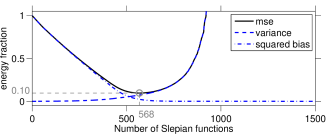
Figure 12: Statistical performance of the truncated Slepian-function internal-field solution to the full-field inversion problem, as computed via eq. (155). The optimal number of Slepian functions ${J}_{\mathrm{opt}}=568$ and the corresponding relative mean-squared error (0.1) are indicated. Layout is as in Fig. 11.

10.4 Case study II: Bandlimited and spectrally flat signal and noise

If the internal field is bandlimited with the same bandwidth $L$ as the internal-field Slepian functions, with a ‘whitish’ spectrum on the planetary surface with power $\mathscr{V}$, and if the external field is bandlimited with the same bandwidth ${L_{o}}$ as the external-field Slepian functions, and with a white spectrum on the outer sphere with power $\mathscr{W}$, eqs (153) and (154) simplify through eq. (132) to the rather digestible forms

$$\text{mse}_{V} =\mathbf{\mathcal{N}}\mathring{\mathcal{G}}_{i{J}}^{\mathcal{T}}\mathring{\mathbf{\Lambda}}_{J}^{-1}\mathring{\mathcal{G}}_{i{J}}+\mathscr{V}\mathring{\mathcal{G}}_{i>{J}}^{\mathcal{T}}\left(\mathring{\mathbf{G}}_{i>{J}}^{\mathrm{T}}\mathring{\mathbf{G}}_{i>{J}}\right)\mathring{\mathcal{G}}_{i>{J}}+\mathscr{W}\mathring{\mathcal{G}}_{i{J}}^{\mathcal{T}}\left(\mathring{\mathbf{G}}_{o{J}}^{\mathrm{T}}\mathring{\mathbf{G}}_{o{J}}\right)\mathring{\mathcal{G}}_{i{J}},$$ (155)

$$\text{mse}_{W} =\mathbf{\mathcal{N}}\mathring{\mathcal{G}}_{o{J}}^{\mathcal{T}}\mathring{\mathbf{\Lambda}}_{J}^{-1}\mathring{\mathcal{G}}_{o{J}}+\mathscr{V}\mathring{\mathcal{G}}_{o>{J}}^{\mathcal{T}}\left(\mathring{\mathbf{G}}_{o>{J}}^{\mathrm{T}}\mathring{\mathbf{G}}_{o>{J}}\right)\mathring{\mathcal{G}}_{o>{J}}+\mathscr{W}\mathring{\mathcal{G}}_{o{J}}^{\mathcal{T}}\left(\mathring{\mathbf{G}}_{i{J}}^{\mathrm{T}}\mathring{\mathbf{G}}_{i{J}}\right)\mathring{\mathcal{G}}_{o{J}}.$$ (156)

To observe the behavior of $\text{mse}_{V}$ depending on the truncation number of Slepian functions ${J}$ for a case similar to the one considered in Section 8, we set $L=100$, ${L_{o}}=10$, ${r_{p}}=6371$ km, ${r_{s}}=6671$ km, ${r_{q}}=6771$ km, and $R=$ North America. To obtain a realistic signal-to-noise ratio at satellite altitude we apply the same principle as earlier to the internal-field power $\mathscr{V}$ and, mutatis mutandis, to the external-field power $\mathscr{W}$. We obtain $\mathscr{V}({r_{p}})=1.1\times 10^{6}\,\mathscr{V}({r_{s}})$ and $\mathscr{W}({r_{q}})=1.5\times 10^{6}\,\mathscr{W}({r_{s}})$. For the example presented in Fig. 12 we chose $\mathscr{V}({r_{s}})=1$, $\mathscr{W}({r_{s}})=0.1$, and $\mathbf{\mathcal{N}}=0.01$. As for the internal-field case described in Section 9.4, we calculate the regional integral of the mean-squared error and normalize it by the regional integral of the signal power. Fig. 12 shows how the bias term decreases with increasing number ${J}$ of Slepian functions. On the other hand, the variance term increases with increasing ${J}$. Together, the variance and bias lead to an optimal number ${J}_{\mathrm{opt}}=568$ that minimizes the mean-squared error at 0.1.

11 Conclusions

We presented two methods to invert for a regional representation of potential fields on a planetary or lunar surface from discrete, regionally available, vector data collected at varying radial positions. The first method only considers internal fields, whereas the second simultaneously inverts for internal and external fields. Both methods are based on systems of functions that arise from solving optimization problems that take the region of data availability and the ensuing downward continuation of the field into account. In our numerical tests we observed that under favorable noise conditions, the estimated internal field faithfully represents the true field within the region of data availability, but is unconstrained outside of this region. Our tests also revealed some of the dangers of not considering external fields when they are present and are not removed by other means. When large-scale external fields were left unaccounted for, the solution contained erroneous small-scale features. Plattner and Simons (2015a) previously applied the internal-field method described in this paper to map the South Polar crustal magnetic field of Mars, after subtracting an external-field model from the data before solving for the internal field. We provided a detailed statistical analysis of both methods, highlighting, in particular, the leakage induced by unaccounted-for data components. For a contrived special case of spectrally flat and bandlimited data, we derived simple analytic expressions for the bias, variance, and mean-squared error of the estimates, which allows us to predict the solution error, which is dominantly controlled by the number of altitude-cognizant gradient vector Slepian functions used in the truncated model expansion. These methods are constructed to maximize the numerical conditioning of the solution under downward continuation from an average satellite altitude. In principle the harmonic continuation matrices could be replaced with any other invertible matrix, such as a noise covariance, and the solution optimized to counteract the influence of noisy measurements, downward continuation, or both. The construction of altitude-cognizant gradient vector Slepian functions necessitates solving an eigenvalue problem which, at large bandwidths, may become computationally expensive. However, for symmetric regions, such as spherical caps, belts or rings, the original eigenvalue problem can be simplified into a set of smaller eigenvalue problems, which can be solved in parallel, dramatically reducing the computational cost.

12 Acknowledgments

This work was sponsored by the National Aeronautics and Space Administration under grant NNX14AM29G. FJS thanks the Institute for Advanced Study for a hospitable environment during the academic year 2014–2015, and the K.U. Leuven for a productive working environment in the summers of 2015 and 2016. The authors thank Nils Olsen, an anonymous referee, and the Associate Editor, Kosuke Heki, for constructive reviews of the submitted manuscript.

Appendix A Computational considerations

In our construction of the altitude-cognizant gradient vector Slepian functions (AC-GVSF) in Sections 4.2 and 5.2 we calculated the eigenvectors of the matrices $\mathbf{K}$ and $\mathring{\mathbf{K}}$, which are of dimensions $(L+1)^{2}\times(L+1)^{2}$ and $[(L+1)^{2}+({L_{o}}+1)^{2}-1]\times[(L+1)^{2}+({L_{o}}+1)^{2}-1]$, respectively. For large $L$, or large ${L_{o}}$, numerical computations may become prohibitively expensive. Fortunately, for symmetric regions such as rings, belts or caps, we can reorder the matrices $\mathbf{K}$ and $\mathring{\mathbf{K}}$ into block-diagonal form, with blocks of maximum size $[L+1]\times[L+1]$, or $[L+{L_{o}}+1]\times[L+{L_{o}}+1]$. Considering that a full eigenvalue decomposition of an $n\times n$ matrix has a numerical complexity of $\mathcal{O}(n^{3})$, the block diagonal reordering significantly reduces the computational costs and allows us to construct altitude-cognizant gradient vector Slepian functions with otherwise prohibitively high maximum spherical-harmonic degrees. For example, a fully populated matrix for internal-field bandlimit $L=500$ and external-field bandlimit ${L_{o}}=10$ containing double-precision floating point numbers would require $(501^{2}+6^{2}-1)^{2}\cdot 8$ bytes $\approx$ 470 GB of memory. Calculating the eigenvalue distribution of such a large matrix would be prohibitively computationally demanding. On the other hand, the largest block-matrix for the symmetric region has dimensions $[L+{L_{o}}+1]\times[L+{L_{o}}+1]$, which would require $(500+5+1)^{2}\cdot 8$ bytes $\approx$ 2 MB. Eigenvalue decompositions for such matrices are feasible even on small computers. The overall memory required for all block-diagonal matrices is $\sum_{m=0}^{\max(L,{L_{o}})}\left[(L+1-m)_{+}+({L_{o}}+1-\max(m,1))_{+}\right]^{2}$, where $(a)_{+}$ is $a$ for $a\geq 0$ and 0 otherwise. For $L=500$ and ${L_{o}}=5$, this amounts to $\approx$ 320 MB, less than 0.1% of the full matrix requirement. Besides, the eigenvalue decompositions only need to be performed on the much smaller ($<2$MB) block matrices. Recently, Bates et al. (2017) proposed a method to calculate approximate classical scalar Slepian functions for generic regions by first obtaining a basis of Slepian functions for a spherical cap surrounding the generic target region and then, in a second step, calculating the Slepian functions for the generic region using the Slepian functions for the spherical cap. Their approach greatly reduces the computational costs. A similar procedure may be implemented for the AC-GVSF.

In Fig. 13 we show examples for such high-maximum-spherical-harmonic internal- and external-field AC-GVSF constructed for a spherical cap of opening angle $1^{\circ}$ centered on the first author’s current favorite pub, with internal-field bandwidth $L=500$, external-field bandwidth ${L_{o}}=10$, and planetary and satellite radii, and external-field radius as discussed in the legend. The left column, above, shows the radial component of the internal field of the best-suited function for this setting, and its power spectral density, below. The right column shows the radial component of the internal field of the 48th-best-suited function, above, and, below, its power spectral density. We constructed these functions on an off-the-shelf desktop computer. We describe our block-diagonalization approaches in Sections A.1 and A.2.

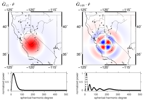
Figure 13: Full-field altitude-cognizant gradient vector Slepian function for a polar cap of opening angle $1^{\circ}$ centered over Peeve’s Public House in Fresno, California with bandwidths $L=500$, and ${L_{o}}=10$, ${r_{p}}=6371$ km, ${r_{q}}=6771$ km, ${r_{s}}=6671$ km. Top left: radial component of highest-eigenvalue internal-field function. Bottom left: Power spectral density of that function. Top right: 48th best internal-field and its power spectral density, bottom right.

A.1 Internal-field altitude-cognizant gradient vector Slepian functions

To reorder the kernel matrix $\mathbf{K}$ of eq. (34) when the region $R$ is a spherical cap, we follow the derivations of Plattner and Simons (2014). As they do, we define $\Theta$ as the half opening angle of the spherical cap. We can describe our internal-field gradient vector spherical harmonics $\boldsymbol{E}_{lm}$ as linear combination of the radial and tangential vector spherical harmonics, $\boldsymbol{P}_{lm}$ and $\boldsymbol{B}_{lm}$, defined by Dahlen and Tromp (1998) as

$$\boldsymbol{P}_{lm}(\boldsymbol{\hat{r}})=\boldsymbol{\hat{r}}\hskip 1.00006ptY_{lm}(\boldsymbol{\hat{r}})\quad\mbox{and}\quad\boldsymbol{B}_{lm}(\boldsymbol{\hat{r}})=\frac{\mbox{\boldmath$\nabla$}_{1}Y_{lm}(\boldsymbol{\hat{r}})}{\sqrt{l(l+1)}},$$ (157)

for $1\leq l\leq L$ and $\-l\leq m\leq l$. For $l=m=0$ we set $\boldsymbol{P}_{00}(\boldsymbol{\hat{r}})=\boldsymbol{\hat{r}}$. Owing to the pointwise orthogonality between $\boldsymbol{P}_{lm}$ and $\boldsymbol{B}_{lm}$, the regional integrals over products of $\boldsymbol{E}_{lm}$ are linear combinations of integrals of products of $\boldsymbol{P}_{lm}$ and $\boldsymbol{B}_{lm}$ with the same spherical-harmonic degrees and orders as the $\boldsymbol{E}_{lm}$,

$$\int_{R}\boldsymbol{E}_{lm}\cdot\boldsymbol{E}_{l^{\prime}m^{\prime}}\,d\Omega=\sqrt{\frac{(l+1)(l^{\prime}+1)}{(2l+1)(2l^{\prime}+1)}}\int_{R}\boldsymbol{P}_{lm}\cdot\boldsymbol{P}_{l^{\prime}m^{\prime}}\,d\Omega+\sqrt{\frac{l\hskip 1.00006ptl^{\prime}}{(2l+1)(2l^{\prime}+1)}}\int_{R}\boldsymbol{B}_{lm}\cdot\boldsymbol{B}_{l^{\prime}m^{\prime}}\,d\Omega.$$ (158)

Plattner and Simons (2014), in their equations (70)–(76), derived the relationships, using a prime to denote differentiation,

$$\int_{R}\boldsymbol{P}_{lm}\cdot\boldsymbol{P}_{l^{\prime}m^{\prime}}\,d\Omega =2\pi\hskip 1.00006pt\delta_{mm^{\prime}}\int_{0}^{\Theta}X_{lm}X_{l^{\prime}m}\sin\theta\,d\theta,$$ (159)

$$\int_{R}\boldsymbol{B}_{lm}\cdot\boldsymbol{B}_{l^{\prime}m^{\prime}}\,d\Omega =\frac{\displaystyle 2\pi\hskip 1.00006pt\delta_{mm^{\prime}}\int_{0}^{\Theta}\left[X^{\prime}_{lm}X^{\prime}_{l^{\prime}m}+m^{2}(\sin\theta)^{-2}X_{lm}X_{l^{\prime}m}\right]\sin\theta\,d\theta}{\displaystyle\sqrt{l(l+1)l^{\prime}(l^{\prime}+1)}}.$$ (160)

Eqs (159)–(160) imply that for $m\neq m^{\prime}$, the regional integral over $\boldsymbol{B}_{lm}\cdot\boldsymbol{P}_{l^{\prime}m^{\prime}}$ is zero, which amounts to the bulk of the entries of matrix $\mathbf{K}$ in eq. (34). We rearrange the non-zero elements using an orthogonal permutation matrix $\mathbf{Q}$ such that, for each $m$, all the corresponding $l,l^{\prime}\geq m$ entries of matrix $\mathbf{K}$ are within one block of size $L-m+1$ and the blocks are collected in a block diagonal matrix $\mathbf{Q}\mathbf{K}\mathbf{Q}^{\mathrm{T}}$. The eigenvectors of $\mathbf{Q}\mathbf{K}\mathbf{Q}^{\mathrm{T}}$ are the permutations $\mathbf{Q}\mathrm{g}$ of the eigenvectors $\mathrm{g}$ defined in eq. (37) with the same eigenvalues, thanks to

$$(\mathbf{Q}\mathbf{K}\mathbf{Q}^{\mathrm{T}})(\mathbf{Q}\mathbf{G})=\mathbf{Q}\mathbf{K}\mathbf{G}=(\mathbf{Q}\mathbf{G})\mathbf{\Lambda}.$$ (161)

For the case or $R=$ polar caps, the entries in each block

$$\mathbf{K}_{m}=\begin{pmatrix}K^{m}_{mm}&\cdots&K^{m}_{mL}\\ \vdots&&\vdots\\ K^{m}_{Lm}&\cdots&K^{m}_{LL}\end{pmatrix}$$ (162)

have analytic expressions that can be obtained from

$$K^{m}_{ll^{\prime}}={r_{p}}^{-2}\sqrt{(l+1)(l^{\prime}+1)(2l+1)(2l^{\prime}+1)}\left(\frac{{r_{s}}}{{r_{p}}}\right)^{-l-l^{\prime}-4}\int_{R}\boldsymbol{E}_{lm}\cdot\boldsymbol{E}_{l^{\prime}m}\,d\Omega,$$ (163)

together with eqs (158)–(160) and the derivations by Simons and Dahlen (2006) and Plattner and Simons (2014). To calculate internal-field AC-GVSF for spherical caps not centered on the North Pole, we can again make use of relationship (161) with $\mathbf{Q}$ defined as the orthogonal spherical-harmonic rotation matrix using the appropriate Euler angles Dahlen and Tromp (1998). We first calculate the eigenvectors for a north-polar cap region with our chosen angle $\Theta$ and then rotate these using the matrix $\mathbf{Q}$. To obtain internal-field AC-GVSF for polar rings we subtract the kernel matrices for the inner cap from the kernel matrices for the large cap.

A.2 Full-field altitude-cognizant gradient vector Slepian functions

To reorder matrix $\mathring{\mathbf{K}}$ in eq. (54) in a similar fashion as in Appendix A.1 we need to also consider the non-vanishing integrals over products of $\boldsymbol{E}_{lm}$ and $\boldsymbol{F}_{lm}$. The following equations describe the relationships between products of $\boldsymbol{F}_{lm}$ and $\boldsymbol{E}_{m}$, and products of $\boldsymbol{P}_{lm}$ and $\boldsymbol{B}_{lm}$,

$$\int_{R}\boldsymbol{F}_{lm}\cdot\boldsymbol{F}_{l^{\prime}m^{\prime}}\,d\Omega=\sqrt{\frac{l\hskip 0.09995ptl^{\prime}}{(2l+1)(2l^{\prime}+1)}}\int_{R}\boldsymbol{P}_{lm}\cdot\boldsymbol{P}_{l^{\prime}m^{\prime}}\,d\Omega+\sqrt{\frac{(l+1)(l^{\prime}+1)}{(2l+1)(2l^{\prime}+1)}}\int_{R}\boldsymbol{B}_{lm}\cdot\boldsymbol{B}_{l^{\prime}m^{\prime}}\,d\Omega,$$ (164)

and

$$\int_{R}\boldsymbol{E}_{lm}\cdot\boldsymbol{F}_{l^{\prime}m^{\prime}}\,d\Omega=\sqrt{\frac{(l+1)l^{\prime}}{(2l+1)(2l^{\prime}+1)}}\int_{R}\boldsymbol{P}_{lm}\cdot\boldsymbol{P}_{l^{\prime}m^{\prime}}\,d\Omega-\sqrt{\frac{l(l^{\prime}+1)}{(2l+1)(2l^{\prime}+1)}}\int_{R}\boldsymbol{B}_{lm}\cdot\boldsymbol{B}_{l^{\prime}m^{\prime}}\,d\Omega.$$ (165)

These integrals are zero unless $m=m^{\prime}$, rendering the matrix $\mathring{\mathbf{K}}$ sparse. To make optimal use of this sparsity and save computational resources in the calculation of its eigenvectors, we reorder the matrix elements into block-diagonal shape using orthogonal transformation. The resulting eigenvectors can be translated back into eigenvectors of the original matrix $\mathring{\mathbf{K}}$ by reordering the vector entries as is explained in eq. (161). To define the individual blocks, we reuse the definition of the matrix entries in eq. (163) and set $K^{im}_{ll^{\prime}}=K^{m}_{ll^{\prime}}$. We also define

$$K^{om}_{ll^{\prime}}={r_{q}}^{-2}\sqrt{l\hskip 1.00006ptl^{\prime}(2l+1)(2l^{\prime}+1)}\left(\frac{{r_{s}}}{{r_{q}}}\right)^{l+l^{\prime}-2}\int_{R}\boldsymbol{F}_{lm}\cdot\boldsymbol{F}_{l^{\prime}m}\,d\Omega,$$ (166)

and

$$K^{iom}_{ll^{\prime}}=({r_{p}}{r_{q}})^{-1}\sqrt{l(l^{\prime}+1)(2l+1)(2l^{\prime}+1)}\left(\frac{{r_{s}}}{{r_{p}}}\right)^{-l-2}\left(\frac{{r_{s}}}{{r_{q}}}\right)^{l^{\prime}-1}\int_{R}\boldsymbol{E}_{lm}\cdot\boldsymbol{F}_{l^{\prime}m}\,d\Omega,$$ (167)

and assemble these elements in the matrices

$$\mathbf{K}^{o}_{m}=\begin{pmatrix}K^{om}_{mm}&\cdots&K^{om}_{m{L_{o}}}\\ \vdots&&\vdots\\ K^{om}_{{L_{o}}m}&\cdots&K^{om}_{{L_{o}}{L_{o}}}\end{pmatrix}\quad\mbox{and}\quad\mathbf{K}^{io}_{m}=\begin{pmatrix}K^{iom}_{mm}&\cdots&K^{iom}_{m{L_{o}}}\\ \vdots&&\vdots\\ K^{iom}_{Lm}&\cdots&K^{iom}_{L{L_{o}}}\end{pmatrix}.$$ (168)

Note that the matrix $\mathbf{K}^{o}_{m}$ is of dimension $[{L_{o}}+1-\max(m,1)]\times[{L_{o}}+1-\max(m,1)]$ while matrix $\mathbf{K}^{io}_{m}$ is of dimension $[L+1-m]\times[{L_{o}}+1-\max(m,1)]$. We collect these matrices in the single block

$$\mathring{\mathbf{K}}_{m}=\begin{pmatrix}\mathbf{K}_{m}&\mathbf{K}^{io}_{m}\\ (\mathbf{K}^{io}_{m})^{\mathrm{T}}&\mathbf{K}^{o}_{m}\end{pmatrix}.$$ (169)

If we elect to calculate internal- and external-field altitude-cognizant gradient vector Slepian functions for spherical caps not centered at the North Pole, we can transform the resulting eigenvectors from the north-polar caps into eigenvectors of spherical caps centered at any other point using orthonormal spherical-harmonic rotation matrices. To obtain internal- and external-field altitude-cognizant gradient vector Slepian functions for spherical-ring regions, we subtract the matrices $\mathring{\mathbf{K}}_{m}$ for the polar cap constituting the inner gap of the ring from the matrices $\mathring{\mathbf{K}}_{m}$ for the larger polar cap. We then transform the resulting eigenvectors using orthonormal spherical-harmonic rotation matrices.

Appendix B Table of Symbols

Symbol	Definition, description, usage	eq.
$V$	(scalar) internal-source potential field, a quantity that we attempt to estimate from the data	(1)
$W$	(scalar) external-source potential field, a quantity that we attempt to estimate from the data	(1)
${r_{p}}$	outer boundary radius for the internal-source field $V$; Earth, planetary or lunar radius	(1)
${r_{s}}$	(average) radial position of the measurement satellite	(1)
${r_{q}}$	inner boundary radius for the external-source field $W$	(1)
$\Omega$	unit sphere, a sphere of unit radius	(1)
$r,\theta,\phi$	radial, colatitudinal, and longitudinal coordinates	(1)
$\boldsymbol{\hat{r}},\boldsymbol{\hat{\theta}},\boldsymbol{\hat{\phi}}$	radial, colatitudinal, and longitudinal unit vectors	(12)
$Y_{lm}$	scalar surface spherical-harmonic; an orthonormal basis function for the potential fields $V$ or $W$	(2)
$l,m$	spherical-harmonic degree, $l\geq 0$ and order $-l\leq m\leq l$	(2)
$v^{r_{p}}_{lm}$	expansion coefficients of the internal-source potential $V({r_{p}}\boldsymbol{\hat{r}})$ in the basis $Y_{lm}(\boldsymbol{\hat{r}})$	(4)
$w^{r_{q}}_{lm}$	expansion coefficients of the external-source potential $W({r_{q}}\boldsymbol{\hat{r}})$ in the basis $Y_{lm}(\boldsymbol{\hat{r}})$	(5)
$L$	maximum spherical-harmonic degree (bandwidth) of the internal-source field $V$ being modeled	(6)
${L_{o}}$	maximum spherical-harmonic degree (bandwidth) of the external field $W$ being modeled	(6)
$\mathrm{v}_{L}^{r_{p}}$	$(L+1)^{2}$-dimensional vector of expansion coefficients $v^{r_{p}}_{lm}$, for $0\leq l\leq L$	(6)
$\mathrm{w}_{L_{o}}^{r_{q}}$	$[({L_{o}}+1)^{2}-1]$-dimensional vector of expansion coefficients $w^{r_{q}}_{lm}$, for $1\leq l\leq{L_{o}}$	(6)
$\mathcal{Y}$	infinite-dimensional vector of all scalar spherical harmonics $Y_{lm}$, for $0\leq l\leq\infty$	(7)
$\mathcal{Y}_{L}$	$(L+1)^{2}$-dimensional vector of the scalar spherical harmonics $Y_{lm}$ for $0\leq l\leq L$	(8)
$\mathcal{Y}_{>L}$	infinite-dimensional vector of the scalar spherical harmonics $Y_{lm}$ for $l\geq L+1$	(8)
$\mathcal{Y}_{L_{o}}$	$[({L_{o}}+1)^{2}-1]$-dimensional vector of the scalar spherical harmonics $Y_{lm}$ for $1\leq l\leq{L_{o}}$	(8)
$\mathcal{Y}_{>{L_{o}}}$	infinite-dimensional vector of all scalar spherical harmonics $Y_{lm}$ for $l\geq{L_{o}}+1$	(8)
$\boldsymbol{B}$	vector-field superposition of the gradients of the internal- and external-source potentials, $\mbox{\boldmath$\nabla$}V+\mbox{\boldmath$\nabla$}W$	(12)
$\boldsymbol{E}_{lm}$	vector surface spherical-harmonic; orthonormal internal-source basis function for $\mbox{\boldmath$\nabla$}V$, for $0\leq l$, $-l\leq m\leq l$	(15)
$\boldsymbol{F}_{lm}$	vector spherical-harmonic; orthonormal external-source basis function for $\mbox{\boldmath$\nabla$}W$, for $1\leq l$ and $-l\leq m\leq l$	(16)
$\boldsymbol{\mathcal{E}},\boldsymbol{\mathcal{F}}$	infinite-dimensional vector of all vector spherical-harmonics $\boldsymbol{E}_{lm}$ for $0\leq l\leq\infty$, or $\boldsymbol{F}_{lm}$ for $1\leq l\leq\infty$	(23)
$\boldsymbol{\mathcal{E}}_{L}$	$(L+1)^{2}$-dimensional vector of the internal-source vector spherical-harmonics $\boldsymbol{E}_{lm}$ for $0\leq l\leq L$	(24)
$\boldsymbol{\mathcal{E}}_{>L}$	infinite-dimensional vector of the internal-source vector spherical-harmonics $\boldsymbol{E}_{lm}$ for $l\geq L+1$	(23)
$\boldsymbol{\mathcal{F}}_{{L_{o}}}$	$[({L_{o}}+1)^{2}-1]$-dimensional vector of the external-source vector spherical-harmonics $\boldsymbol{F}_{lm}$ for $1\leq l\leq{L_{o}}$	(24)
$\boldsymbol{\mathcal{F}}_{>{L_{o}}}$	infinite-dimensional vector of the external-source vector spherical-harmonics $\boldsymbol{F}_{lm}$ for $l\geq{L_{o}}+1$	(23)
$A_{l}(r)$	upward-continuation factor for internal-source fields, from planetary surface ${r_{p}}$ up to $r$, for $l\geq 0$	(17)
$\breve{A}_{l}(r)$	downward-continuation factor for external-source fields, from inner boundary ${r_{q}}$ down to $r$, for $l\geq 1$	(18)
$\mathbf{A}(r)$	diagonal matrix containing the $A_{l}(r)$, for a context-dependent range of $l\geq 0$	(19)
$\mathbf{\breve{A}}(r)$	diagonal matrix containing the $\breve{A}_{l}(r)$, for a context-dependent range of $l\geq 1$	(20)
$\mathbf{A}$	silent notation, whereby is meant $\mathbf{A}({r_{s}})$, evaluated at the (radial average of the) satellite position	(21)
$\mathbf{\breve{A}}$	silent notation, whereby is meant $\mathbf{\breve{A}}({r_{s}})$, evaluated at the (radial average of the) satellite position	(22)
$\boldsymbol{d}(r\boldsymbol{\hat{r}})$	vector-valued function with the data collected by the satellite	(29)
$\boldsymbol{n}(r\boldsymbol{\hat{r}})$	vector-valued function with observational noise contaminating the data	(29)
$\boldsymbol{d},\boldsymbol{n}$	shorthand for the data and noise functions at average satellite altitude, $\boldsymbol{d}=\boldsymbol{d}({r_{s}}\boldsymbol{\hat{r}})$ and $\boldsymbol{n}=\boldsymbol{n}({r_{s}}\boldsymbol{\hat{r}})$	(30)
$R$	region of data availability on the unit sphere $\Omega$; target region for Slepian-function concentration; model domain	(29)
$\mathrm{\tilde{v}}^{r_{p}}_{L}$	estimated internal-source coefficient vector; minimizer of internal-source least-squares data functional on $R$	(31)
$\mathrm{\tilde{w}}_{L_{o}}^{r_{q}}$	estimated external-source coefficient vector; minimizer of internal/external data misfit functional over $R$	(52)
$\mathbf{K}$	inner-product (over $R$, hence “localization”) matrix of upward-continued inner-source vector harmonics $\mathbf{A}\boldsymbol{\mathcal{E}}_{L}$	(34)
$\mathring{\mathbf{K}}$	inner-product matrix of up/downward-continued internal/external-source vector harmonics $\mathbf{A}\boldsymbol{\mathcal{E}}_{L}$ and $\mathbf{\breve{A}}\boldsymbol{\mathcal{F}}_{{L_{o}}}$	(54)
$\mathbf{\Lambda}$	diagonal matrix containing the $(L+1)^{2}$ eigenvalues of $\mathbf{K}$: the “optimization” or “concentration” factors $\lambda_{\alpha}$	(35)
$\mathring{\mathbf{\Lambda}}$	diagonal matrix containing the $[(L+1)^{2}+({L_{o}}+1)^{2}-1]$ eigenvalues of $\mathring{\mathbf{K}}$: the optimization factors $\mathring{\lambda}_{\alpha}$	(55)
$\mathbf{\Lambda}_{J}$	diagonal matrix containing the ${J}$ largest eigenvalues $\lambda_{\alpha}$ of $\mathbf{K}$; ${J}\times{J}$-dimensional truncation of $\mathbf{\Lambda}$	(36)
$\mathring{\mathbf{\Lambda}}_{J}$	diagonal matrix containing the ${J}$ largest eigenvalues $\mathring{\lambda}_{\alpha}$ of $\mathring{\mathbf{K}}$; ${J}\times{J}$-dimensional truncation of $\mathring{\mathbf{\Lambda}}$	(57)
$\mathbf{G}$	eigenvector matrix of $\mathbf{K}$; columns $\mathrm{g}_{\alpha}$ contain the $Y_{lm}$-expansion coefficients $g_{lm,\alpha}$ of scalar functions $G_{\alpha}$	(35)
$\mathring{\mathbf{G}}$	eigenvector matrix of $\mathring{\mathbf{K}}$; columns $\mathring{\mathrm{g}}_{\alpha}$ with $Y_{lm}$-coefficients $\mathring{g}_{i\,lm,\alpha}$ and $g_{o\,lm,\alpha}$ of scalar $\mathring{G}_{i\alpha}$ and $\mathring{G}_{o\alpha}$	(55)
$\mathbf{G}_{J}$	$(L+1)^{2}\times{J}$ matrix with th ${J}$ best eigenvectors of $\mathbf{K}$; restriction of $\mathbf{G}$ to its first ${J}$ columns	(36)
$\mathring{\mathbf{G}}_{J}$	$[(L+1)^{2}+({L_{o}}+1)^{2}-1]\times{J}$ matrix with the ${J}$ best eigenvectors of $\mathring{\mathbf{K}}$; column-restriction of $\mathring{\mathbf{G}}$	(56)
$\mathring{\mathbf{G}}_{i}$	$(L+1)^{2}\times[(L+1)^{2}+({L_{o}}+1)^{2}-1]$-dimensional matrix of columns $\mathring{\mathrm{g}}_{i\alpha}$ with coefficients $\mathring{g}_{i\,lm,\alpha}$ of $\mathring{G}_{i\alpha}$	(58)
$\mathring{\mathbf{G}}_{o}$	$[({L_{o}}+1)^{2}-1]\times[(L+1)^{2}+({L_{o}}+1)^{2}-1]$-dimensional matrix of columns $\mathring{\mathrm{g}}_{o\alpha}$ with the $g_{o\,lm,\alpha}$ of $\mathring{G}_{o\alpha}$	(58)
$\mathring{\mathbf{G}}_{i{J}},\mathring{\mathbf{G}}_{o{J}}$	restrictions of $\mathring{\mathbf{G}}_{i}$ and $\mathring{\mathbf{G}}_{o}$ to their first ${J}$ columns	(58)
$\lambda_{\alpha}$	eigenvalues of $\mathbf{K}$, in descending order, for $1\leq\alpha\leq(L+1)^{2}$; the diagonal elements of $\mathbf{\Lambda}$	(35)
$\mathring{\lambda}_{\alpha}$	eigenvalues of $\mathring{\mathbf{K}}$, in descending order, for $1\leq\alpha\leq[(L+1)^{2}+({L_{o}}+1)^{2}-1]$; the diagonal elements of $\mathring{\mathbf{\Lambda}}$	(55)
$\mathrm{g}_{\alpha}$	$(L+1)^{2}$-dimensional column vector, the $\alpha$-th column of $\mathbf{G}$, contains the $g_{lm,\alpha}$	(37)
$\mathring{\mathrm{g}}_{\alpha}$	$[(L+1)^{2}+({L_{o}}+1)^{2}-1]$-dimensional column vector, the $\alpha$-th column of $\mathring{\mathbf{G}}$; also $\mathring{\mathrm{g}}_{\alpha}=\begin{pmatrix}\mathring{\mathrm{g}}_{i\alpha}^{\mathrm{T}}&\mathring{\mathrm{g}}_{o\alpha}^{\mathrm{T}}\end{pmatrix}^{\mathrm{T}}$	(56)
$\mathring{\mathrm{g}}_{i\alpha}$	$(L+1)^{2}$-dimensional column vector, the $(L+1)^{2}$ first elements of $\mathring{\mathrm{g}}_{\alpha}$, contains the $\mathring{g}_{i\,lm,\alpha}$	(58)
$\mathring{\mathrm{g}}_{o\alpha}$	$[({L_{o}}+1)^{2}-1]$-dimensional column vector, the $({L_{o}}+1)^{2}-1$ last elements of of $\mathring{\mathrm{g}}_{\alpha}$, contains the $\mathring{g}_{o\,lm,\alpha}$	(58)
$g_{lm,\alpha}$	spherical-harmonic expansion coefficients of the $G_{\alpha}$: the elements of $\mathrm{g}_{\alpha}$	(38)
$\mathring{g}_{i\,lm,\alpha}$	spherical-harmonic expansion coefficients of the $\mathring{G}_{i\alpha}$: first $(L+1)^{2}$ scalar elements of $\mathring{\mathrm{g}}_{\alpha}$; the elements of $\mathring{\mathrm{g}}_{i\alpha}$	(58)
$\mathring{g}_{o\,lm,\alpha}$	spherical-harmonic expansion coefficients of the $\mathring{G}_{o\alpha}$: last $({L_{o}}+1)^{2}-1$ elements of $\mathring{\mathrm{g}}_{\alpha}$; the elements of $\mathring{\mathrm{g}}_{o\alpha}$	(58)
AC-GVSF	abbreviation of ‘altitude-cognizant gradient vector Slepian functions’ in their various forms	passim
$\mathscr{G}_{\alpha}(l)$	spherical-harmonic power spectrum of $G_{\alpha}(\boldsymbol{\hat{r}})$ at the degree $l$; mean-squared value of the coefficients $g_{lm,\alpha}$	(38)
$G_{\alpha}$	scalar AC-GVSF; spherical-harmonic expansions of the eigenvectors of the internal-field matrix $\mathbf{K}$	(39)
$\mathring{G}_{i\alpha}$	scalar internal-source AC-GVSF; expansions of internal-source eigenvectors $\mathring{\mathbf{G}}_{i}$ of the full-field matrix $\mathring{\mathbf{K}}$	(61)
$\mathring{G}_{o\alpha}$	scalar external-source AC-GVSF; expansions of external-source eigenfunctions $\mathring{\mathbf{G}}_{o}$ of the full-field matrix $\mathring{\mathbf{K}}$	(62)
$\boldsymbol{G}_{\alpha}$	vector internal-source AC-GVSF for the internal-source matrix $\mathbf{K}$, evaluated on the planetary surface ${r_{p}}$	(41)
$\mathring{\boldsymbol{G}}_{i\alpha}$	vector internal-source AC-GVSF for the full-field matrix $\mathring{\mathbf{K}}$, evaluated on the planetary surface ${r_{p}}$	(65)
$\mathring{\boldsymbol{G}}_{o\alpha}$	vector external-source AC-GVSF for the full-field matrix $\mathring{\mathbf{K}}$, at inner boundary of the external-source field ${r_{q}}$	(66)
$\boldsymbol{G}_{\uparrow\alpha}$	vector internal-source AC-GVSF: the $\boldsymbol{G}_{\alpha}$ after upward-continuation from ${r_{p}}$ to average satellite altitude ${r_{s}}$	(43)
$\mathring{\boldsymbol{G}}_{i\uparrow\alpha}$	vector internal-source AC-GVSF: the $\mathring{\boldsymbol{G}}_{i\alpha}$ after upward-continuation from ${r_{p}}$ to average satellite altitude ${r_{s}}$	(69)
$\mathring{\boldsymbol{G}}_{o\uparrow\alpha}$	vector external-source AC-GVSF: the $\mathring{\boldsymbol{G}}_{o\alpha}$ after downward-continuation from ${r_{q}}$ to average satellite altitude ${r_{s}}$	(70)
$\mathring{\boldsymbol{G}}_{\uparrow\alpha}$	vector full-field AC-GVSF, the summed $\mathring{\boldsymbol{G}}_{i\alpha}$ and $\mathring{\boldsymbol{G}}_{o\alpha}$, evaluated at average satellite altitude ${r_{s}}$	(71)
$\mathcal{G},\mathcal{G}_{J}$	vectors with the $G_{\alpha}$ for $1\leq\alpha\leq(L+1)^{2}$ or $1\leq\alpha\leq{J}$; their complement is $\mathcal{G}_{>{J}}$	(40)
$\mathring{\mathcal{G}}_{i},\mathring{\mathcal{G}}_{i{J}}$	vectors with the $\mathring{G}_{i\alpha}$ for $1\leq\alpha\leq(L+1)^{2}+({L_{o}}+1)^{2}-1$ or $1\leq\alpha\leq{J}$; their complement is $\mathring{\mathcal{G}}_{i>{J}}$	(63)
$\mathring{\mathcal{G}}_{o},\mathring{\mathcal{G}}_{o{J}}$	vectors with the $\mathring{G}_{o\alpha}$ for $1\leq\alpha\leq(L+1)^{2}+({L_{o}}+1)^{2}-1$ or $1\leq\alpha\leq{J}$; their complement is $\mathring{\mathcal{G}}_{o>{J}}$	(64)
$\boldsymbol{\mathcal{G}},\boldsymbol{\mathcal{G}}_{J}$	vectors with the $\boldsymbol{G}_{\alpha}$ for $1\leq\alpha\leq(L+1)^{2}$ or $1\leq\alpha\leq{J}$, complemented by $\boldsymbol{\mathcal{G}}_{>{J}}$	(42)
$\mathring{\boldsymbol{\mathcal{G}}}_{i},\mathring{\boldsymbol{\mathcal{G}}}_{i{J}}$	vectors with the $\mathring{\boldsymbol{G}}_{i\alpha}$ for $1\leq\alpha\leq(L+1)^{2}+({L_{o}}+1)^{2}-1$ or $1\leq\alpha\leq{J}$, complemented by $\mathring{\boldsymbol{\mathcal{G}}}_{i>{J}}$	(67)
$\mathring{\boldsymbol{\mathcal{G}}}_{o},\mathring{\boldsymbol{\mathcal{G}}}_{o{J}}$	vectors with the $\mathring{\boldsymbol{G}}_{o\alpha}$ for $1\leq\alpha\leq(L+1)^{2}+({L_{o}}+1)^{2}-1$ or $1\leq\alpha\leq{J}$, complemented by $\mathring{\boldsymbol{\mathcal{G}}}_{o>{J}}$	(68)
$\boldsymbol{\mathcal{G}}_{\uparrow},\boldsymbol{\mathcal{G}}_{\uparrow{J}}$	vectors with the $\boldsymbol{G}_{\uparrow\alpha}$ for $1\leq\alpha\leq(L+1)^{2}$ or $1\leq\alpha\leq{J}$, complemented by $\boldsymbol{\mathcal{G}}_{\uparrow>{J}}$	(43)
$\mathring{\boldsymbol{\mathcal{G}}}_{i\uparrow},\mathring{\boldsymbol{\mathcal{G}}}_{i\uparrow{J}}$	vectors with the $\mathring{\boldsymbol{G}}_{i\uparrow\alpha}$ for $1\leq\alpha\leq(L+1)^{2}+({L_{o}}+1)^{2}-1$ or $1\leq\alpha\leq{J}$, complemented by $\mathring{\boldsymbol{\mathcal{G}}}_{i\uparrow>{J}}$	(69)
$\mathring{\boldsymbol{\mathcal{G}}}_{o\uparrow},\mathring{\boldsymbol{\mathcal{G}}}_{o\uparrow{J}}$	vectors with the $\mathring{\boldsymbol{G}}_{o\uparrow\alpha}$ for $1\leq\alpha\leq(L+1)^{2}+({L_{o}}+1)^{2}-1$ or $1\leq\alpha\leq{J}$, complemented by $\mathring{\boldsymbol{\mathcal{G}}}_{o\uparrow>{J}}$	(70)
$\boldsymbol{\mathcal{G}}_{\downarrow},\boldsymbol{\mathcal{G}}_{\downarrow{J}}$	vectors containing downward-continued vector internal-source AC-GVSF	(102)
$\mathring{\boldsymbol{\mathcal{G}}}_{i\downarrow},\mathring{\boldsymbol{\mathcal{G}}}_{i\downarrow{J}}$	vectors containing downward-continued internal-source functions from the set of full-field AC-GVSF	(122)
$\mathring{\boldsymbol{\mathcal{G}}}_{o\downarrow},\mathring{\boldsymbol{\mathcal{G}}}_{o\downarrow{J}}$	vectors containing downward-continued external-source functions from the set of full-field AC-GVSF	(123)
$s_{\alpha}$	expansion coefficients of internal-source potential $V({r_{p}}\boldsymbol{\hat{r}})$ in the scalar AC-GVSF basis $G_{\alpha}(\boldsymbol{\hat{r}})$	(45)
$\mathring{s}_{i\alpha}$	expansion coefficients of internal-source potential $V({r_{p}}\boldsymbol{\hat{r}})$ in the scalar AC-GVSF basis $\mathring{G}_{i\alpha}(\boldsymbol{\hat{r}})$	(74)
$\mathring{s}_{o\alpha}$	expansion coefficients of external-source potential $W({r_{q}}\boldsymbol{\hat{r}})$ in the scalar AC-GVSF basis $\mathring{G}_{o\alpha}(\boldsymbol{\hat{r}})$	(76)
$t_{\alpha}$	sum of the coefficients $\mathring{s}_{i\alpha}$ and $\mathring{s}_{o\alpha}$	(78)
$\mathrm{s}$	$(L+1)^{2}$-dimensional vector of expansion coefficients $s_{\alpha}$, for $1\leq\alpha\leq(L+1)^{2}$	(44)
$\mathring{\mathrm{s}}_{i}$	$[(L+1)^{2}+({L_{o}}+1)^{2}-1]$-dimensional vector of coefficients $\mathring{s}_{i\alpha}$, for $1\leq\alpha\leq(L+1)^{2}+({L_{o}}+1)^{2}-1$	(72)
$\mathring{\mathrm{s}}_{o}$	$[(L+1)^{2}+({L_{o}}+1)^{2}-1]$-dimensional vector of coefficients $\mathring{s}_{o\alpha}$, for $1\leq\alpha\leq(L+1)^{2}+({L_{o}}+1)^{2}-1$	(73)
$\mathrm{t}$	$[(L+1)^{2}+({L_{o}}+1)^{2}-1]$-dimensional vector of coefficients $\mathring{s}_{i\alpha}+\mathring{s}_{o\alpha}$	(78)
$\mathrm{s}_{J}$	vector containing the coefficients $s_{\alpha}$ for $1\leq\alpha\leq{J}$, approximating $V({r_{p}}\boldsymbol{\hat{r}})$ over $R\subset\Omega$	(46)
$\mathring{\mathrm{s}}_{i{J}}$	vector containing the coefficients $\mathring{s}_{i\alpha}$ for $1\leq\alpha\leq{J}$, approximating $V({r_{p}}\boldsymbol{\hat{r}})$ over $R\subset\Omega$	(75)
$\mathring{\mathrm{s}}_{o{J}}$	vector containing the coefficients $\mathring{s}_{o\alpha}$ for $1\leq\alpha\leq{J}$, approximating $W({r_{q}}\boldsymbol{\hat{r}})$ over $R\subset\Omega$	(77)
$\mathrm{t}_{J}$	vector containing the coefficients $t_{\alpha}$ for $1\leq\alpha\leq{J}$	(78)
$\tilde{\mathrm{s}}_{{J}}$	truncated estimator of the ${J}$ first terms in the coefficient vector $\mathrm{s}$, using ${J}$ terms of the inner-source AC-GVSF	(48)
$\mathrm{\tilde{t}}_{J}$	truncated estimator of the ${J}$ first terms in the coefficient vector $\mathrm{t}$, using ${J}$ terms of the full-field AC-GVSF	(80)
$\tilde{s}_{\alpha}$	an element of $\tilde{\mathrm{s}}_{{J}}$; expansion coefficient of the truncated estimate $\tilde{V}_{J}({r_{p}}\boldsymbol{\hat{r}})$ in the AC-GVSF basis $G_{\alpha}(\boldsymbol{\hat{r}})$	(50)
$\tilde{t}_{\alpha}$	an element of $\mathrm{\tilde{t}}_{J}$; expansion coefficient of the estimate $\tilde{V}_{J}({r_{p}}\boldsymbol{\hat{r}})$ in the internal-source AC-GVSF basis $\mathring{G}_{i\alpha}(\boldsymbol{\hat{r}})$;	(82)
	also: expansion coefficient of the estimate $\tilde{W}_{J}({r_{q}}\boldsymbol{\hat{r}})$ in the external-source AC-GVSF basis $\mathring{G}_{o\alpha}(\boldsymbol{\hat{r}})$	(83)
$\tilde{V}_{J}({r_{p}}\boldsymbol{\hat{r}})$	estimate of the internal-source field $V$, in the truncated AC-GVSF basis, considering internal-source fields;	(50)
	estimate of the internal-source field $V$, in the truncated AC-GVSF basis, considering internal/external fields	(82)
$\tilde{W}_{J}({r_{q}}\boldsymbol{\hat{r}})$	estimate of the external field $W$, in the truncated AC-GVSF basis, considering internal and external fields	(83)
$k$	number of vector-valued observations available: a discrete data set on $R\subset\Omega$; for a total of $3k$ components	(84)
$\mathsf{d}$	vector with the three spherical vector components of the field observed at each of the positions $r_{i}\boldsymbol{\hat{r}}_{i}$, $1\leq i\leq k$	(86)
$\boldsymbol{\mathsf{E}}_{\Uparrow}$	$[(L+1)^{2}\times 3k]$-dimensional matrix with the upward-continued $\boldsymbol{E}_{lm}$ harmonics evaluated at the data	(84)
$\boldsymbol{\mathsf{F}}_{\Uparrow}$	$[(L+1)^{2}\times 3k]$-dimensional matrix with the downward-continued $\boldsymbol{F}_{lm}$ harmonics at the data locations	(91)
${\boldsymbol{\mathsf{G}}}_{\Uparrow J}$	$[{J}\times 3k]$-dimensional matrix containing the internal-source AC-GVSF $\boldsymbol{\mathcal{G}}_{\uparrow{J}}$ evaluated at the data locations	(85)
$\mathring{\boldsymbol{\mathsf{G}}}_{\Uparrow{J}}$	$[{J}\times 3k]$-dimensional matrix containing the full-field AC-GVSF $\mathring{\boldsymbol{\mathcal{G}}}_{\uparrow{J}}$ evaluated at the data locations	(92)
$\hat{\mathrm{s}}_{J}$	discrete-data truncated estimator of the ${J}$ first terms in the coefficient vector $\mathrm{s}$; the $\hat{s}_{\alpha}$ for $1\leq\alpha\leq{J}$	(86)
$\mathrm{\hat{t}}_{J}$	discrete-data truncated estimator of the ${J}$ first terms in the coefficient vector $\mathrm{t}$; the $\hat{t}_{\alpha}$ for $1\leq\alpha\leq{J}$	(93)
$\hat{s}_{\alpha}$	an element of $\hat{\mathrm{s}}_{J}$; expansion coefficient of $\hat{V}_{J}({r_{p}}\boldsymbol{\hat{r}})$ in the AC-GVSF basis $G_{\alpha}(\boldsymbol{\hat{r}})$	(89)
$\hat{t}_{\alpha}$	an element of $\mathrm{\hat{t}}_{J}$; expansion coefficient of $\hat{V}_{J}({r_{p}}\boldsymbol{\hat{r}})$ and $\hat{W}_{J}({r_{q}}\boldsymbol{\hat{r}})$ in the AC-GVSF basis $\mathring{G}_{i\alpha}(\boldsymbol{\hat{r}})$ and $\mathring{G}_{o\alpha}(\boldsymbol{\hat{r}})$	(97)
$\mathsf{r}$	vector with data residuals obtained after comparison with predictions derived from the truncated estimator $\hat{\mathrm{s}}_{J}$	(87)
$\mathring{\mathsf{r}}$	vector with data residuals obtained after comparison with predictions derived from the truncated estimator $\mathrm{\hat{t}}_{J}$	(95)
$\boldsymbol{\mathsf{R}}$	$[3k\times 3k]$-dimensional diagonal matrix containing (thresholded) residuals $\mathsf{r}$	(88)
$\mathring{\boldsymbol{\mathsf{R}}}$	$[3k\times 3k]$-dimensional diagonal matrix containing (thresholded) residuals $\mathring{\mathsf{r}}$	(94)
$\hat{V}_{J}({r_{p}}\boldsymbol{\hat{r}})$	truncated-AC-GVSF estimate of the internal-source field $V$, variable-altitude discrete data, inner-source fields;	(89)
	truncated-AC-GVSF estimate of internal-source field $V$, variable-altitude discrete data, internal/external fields	(96)
$\hat{W}_{J}({r_{q}}\boldsymbol{\hat{r}})$	truncated-AC-GVSF estimate of external field $W$, from variable-altitude discrete data, internal/external fields	(97)
$\boldsymbol{H}_{\uparrow\alpha,>L}$	spacelimited, infinitely-wideband AC-GVSF made from the degrees $l>L$ after truncation of the $\boldsymbol{G}_{\uparrow\alpha}$ to $R$	(111)
$\boldsymbol{\mathcal{H}}_{\uparrow J,>L}$	vector collecting the $\boldsymbol{H}_{\uparrow\alpha,>L}$ for $1\leq\alpha\leq{J}$	(111)
$\mathrm{h}_{\uparrow\alpha,>L}$	vector containing the $\boldsymbol{E}_{lm}$ expansion coefficients of the spacelimited $\boldsymbol{H}_{\uparrow\alpha J,>L}$	(112)
$\mathring{\boldsymbol{H}}^{\boldsymbol{\mathcal{E}}}_{\uparrow\alpha,>L}$	spacelimited, wideband AC-GVSF made from the $\boldsymbol{E}_{lm}$ components, for $l>L$, of the $\mathring{\boldsymbol{G}}_{\uparrow\alpha}$ truncated to $R$	(135)
${\mathring{\boldsymbol{\mathcal{H}}}}^{\boldsymbol{\mathcal{E}}}_{\uparrow{J},>L}$	vector collecting the $\mathring{\boldsymbol{H}}^{\boldsymbol{\mathcal{E}}}_{\uparrow\alpha,>L}$ for $1\leq\alpha\leq{J}$	(135)
${\mathring{\mathrm{h}}}^{\boldsymbol{\mathcal{E}}}_{\uparrow\alpha,>L}$	vector containing the $\boldsymbol{E}_{lm}$ expansion coefficients of the spacelimited $\mathring{\boldsymbol{H}}^{\boldsymbol{\mathcal{E}}}_{\uparrow\alpha J,>L}$	(137)
$\mathring{\boldsymbol{H}}^{\boldsymbol{\mathcal{F}}}_{\uparrow\alpha,>{L_{o}}}$	spacelimited, wideband AC-GVSF made from the $\boldsymbol{F}_{lm}$ components, for $l>L$, of the $\mathring{\boldsymbol{G}}_{\uparrow\alpha}$ truncated to $R$	(136)
${\mathring{\boldsymbol{\mathcal{H}}}}^{\boldsymbol{\mathcal{F}}}_{\uparrow{J},>{L_{o}}}$	vector collecting the $\mathring{\boldsymbol{H}}^{\boldsymbol{\mathcal{F}}}_{\uparrow\alpha,>{L_{o}}}$ for $1\leq\alpha\leq{J}$	(136)
${\mathring{\mathrm{h}}}^{\boldsymbol{\mathcal{F}}}_{\uparrow\alpha,>{L_{o}}}$	vector containing the $\boldsymbol{F}_{lm}$ expansion coefficients of the spacelimited $\mathring{\boldsymbol{H}}^{\boldsymbol{\mathcal{F}}}_{\uparrow\alpha J,>L}$	(138)
$b$	spatial bias of the truncated AC-GVSF estimator $\tilde{V}_{J}({r_{p}}\boldsymbol{\hat{r}})$ considering internal-source fields only	(117)
$b_{V}$	first portion of the spatial bias of the truncated AC-GVSF estimator $\tilde{V}_{J}({r_{p}}\boldsymbol{\hat{r}})$ solving the full-field problem	(146)
$b_{VW}$	second portion of the spatial bias of the truncated AC-GVSF estimator $\tilde{V}_{J}({r_{p}}\boldsymbol{\hat{r}})$ solving the full-field problem	(148)
$b_{W}$	first portion of the spatial bias of the truncated AC-GVSF estimator $\tilde{W}_{J}({r_{q}}\boldsymbol{\hat{r}})$ solving the full-field problem	(147)
$b_{WV}$	second portion of the spatial bias of the truncated AC-GVSF estimator $\tilde{W}_{J}({r_{q}}\boldsymbol{\hat{r}})$ solving the full-field problem	(149)
$\mathscr{V}$	spatial two-point covariance of the scalar internal-source signal $V({r_{p}}\boldsymbol{\hat{r}})$	(118)
$\mathscr{W}$	spatial two-point covariance of the scalar external-source signal $W({r_{q}}\boldsymbol{\hat{r}})$	(151)
$\mathbf{\mathcal{N}}$	spatial two-point covariance of the vector-valued data noise $\boldsymbol{n}({r_{s}}\boldsymbol{\hat{r}})$	(119)
$\mathrm{mse}$	mean-squared estimation error of the truncated AC-GVSF estimate $\tilde{V}_{J}({r_{p}}\boldsymbol{\hat{r}})$ for the internal-source field	(120)
$\mathrm{mse}_{V}$	mean-squared error of the truncated AC-GVSF internal-source estimate $\tilde{V}_{J}({r_{p}}\boldsymbol{\hat{r}})$ solving the full-field problem	(153)
$\mathrm{mse}_{W}$	mean-squared error of the truncated AC-GVSF external-source estimate $\tilde{W}_{J}({r_{q}}\boldsymbol{\hat{r}})$ solving full-field problem	(154)

References

- Albee et al. (2001) Albee, A. L., Arvidson, R. E., Palluconi, F., and Thorpe, T. (2001). Overview of the Mars Global Surveyor mission. J. Geophys. Res., 106(E10), 23291–23316, doi: 10.1029/2000JE001306.
- Albertella et al. (1999) Albertella, A., Sansò, F., and Sneeuw, N. (1999). Band-limited functions on a bounded spherical domain: the Slepian problem on the sphere. J. Geod., 73, 436–447.
- Amirbekyan et al. (2008) Amirbekyan, A., Michel, V., and Simons, F. J. (2008). Parameterizing surface-wave tomopgraphic models with harmonic spherical splines. Geophys. J. Int., 174(2), 617–628, doi: 10.1111/j.1365–246X.2008.03809.x.
- Aster et al. (2013) Aster, R. C., Borchers, B., and Thurber, C. H. (2013). Parameter Estimation and Inverse Problems. Elsevier Academic Press, San Diego, Calif.
- Backus (1986) Backus, G. (1986). Poloidal and toroidal fields in geomagnetic field modeling. Rev. Geophys., 24(1), 75–109, doi: 10.1029/RG024i001p00075.
- Backus et al. (1996) Backus, G. E., Parker, R. L., and Constable, C. G. (1996). Foundations of Geomagnetism. Cambridge Univ. Press, Cambridge, UK.
- Bates et al. (2017) Bates, A., Khalid, Z., and Kennedy, R. (2017). Efficient computation of Slepian functions for arbitrary regions on the sphere. IEEE Trans. Signal Process., page under review.
- Baur and Sneeuw (2011) Baur, O. and Sneeuw, N. (2011). Assessing Greenland ice mass loss by means of point-mass modeling: a viable methodology. J. Geod., 85(9), 607–615, doi: 10.1007/s00190–011–0463–1.
- Blakely (1995) Blakely, R. J. (1995). Potential Theory in Gravity and Magnetic Applications. Cambridge Univ. Press, New York.
- Bölling and Grafarend (2005) Bölling, K. and Grafarend, E. W. (2005). Ellipsoidal spectral properties of the Earth’s gravitational potential and its first and second derivatives. J. Geod., 79(6–7), 300–330, doi: 10.1007/s00190–005–0465–y.
- Connerney (2015) Connerney, J. E. P. (2015). Planetary magnetism. In T. Spohn, editor, Treatise on Geophysics, volume 10, pages 195–237, doi: 10.1016/B978–0–444–53802–4.00171–8. Elsevier, Amsterdam, Neth., 2 edition.
- Cox and Hinkley (1974) Cox, D. R. and Hinkley, D. V. (1974). Theoretical Statistics. Chapman and Hall, London, UK.
- Dahlen and Tromp (1998) Dahlen, F. A. and Tromp, J. (1998). Theoretical Global Seismology. Princeton Univ. Press, Princeton, N.J.
- Davison and Hinkley (1997) Davison, A. C. and Hinkley, D. V. (1997). Bootstrap Methods and Their Application. Cambridge Univ. Press, Cambridge, UK.
- Eshagh (2009) Eshagh, M. (2009). Spatially restricted integrals in gradiometric boundary value problems. Artif. Sat., 44(4), 131–148, doi: 10.2478/v10018–009–0025–4.
- Farquharson and Oldenburg (1998) Farquharson, C. G. and Oldenburg, D. W. (1998). Non-linear inversion using general measures of data misfit and model structure. Geophys. J. Int., 134, 213–227, doi: 10.1046/j.1365–246x.1998.00555.x.
- Freeden and Michel (1999) Freeden, W. and Michel, V. (1999). Constructive approximation and numerical methods in geodetic research today — an attempt at a categorization based on an uncertainty principle. J. Geod., 73(9), 452–465.
- Freeden and Schreiner (2009) Freeden, W. and Schreiner, M. (2009). Spherical Functions of Mathematical Geosciences: A Scalar, Vectorial, and Tensorial Setup. Springer, Berlin, Germany.
- Freeden et al. (2016) Freeden, W., Michel, V., and Simons, F. J. (2016). Spherical-harmonics based special function systems and constructive approximation methods. In W. Freeden, editor, Handbook of Mathematical Geodesy, page under review. Springer, Berlin, Germany.
- Gauss (1839) Gauss, C. F. (1839). Allgemeine Theorie des Erdmagnetismus. In C. F. Gauss and W. Weber, editors, Resultate aus den Beobachtungen des magnetischen Vereins im Jahre 1838, pages 1–57. Weidmannsche Buchhandlung, Leipzig, Germany.
- Gerhards (2011) Gerhards, C. (2011). Spherical decompositions in a global and local framework: theory and an application to geomagnetic modeling. Intern. J. Geomath., 1(2), 205–256, doi: 10.1007/s13137–010–0011–9.
- Gerhards (2012) Gerhards, C. (2012). Locally supported wavelets for the separation od spherical vector fields with respect to their sources. Int. J. Wavelets Multiresolut. Inf. Process., 10(4), 1250034, doi: 10.1142/S0219691312500348.
- Gerhards (2014) Gerhards, C. (2014). A combination of downward continuation and local approximation for harmonic potentials. 30, 085004, doi: 10.1088/0266–5611/30/8/08500.
- Holschneider et al. (2003) Holschneider, M., Chambodut, A., and Mandea, M. (2003). From global to regional analysis of the magnetic field on the sphere using wavelet frames. Phys. Earth Planet. Inter., 135, 107–124.
- Jahn and Bokor (2014) Jahn, K. and Bokor, N. (2014). Revisiting the concentration problem of vector fields within a spherical cap: A commuting differential operator solution. J. Fourier Anal. Appl., 288(2), 421–451.
- Kaula (1967) Kaula, W. M. (1967). Theory of statistical analysis of data distributed over a sphere. Rev. Geophys., 5(1), 83–107, doi: 10.1029/RG005i001p00083.
- Kaula (1968) Kaula, W. M. (1968). An Introduction to Planetary Physics. The Terrestrial Planets. Wiley, New York.
- Lambeck (1988) Lambeck, K. (1988). Geophysical Geodesy. Oxford Univ. Press, New York.
- Langel and Estes (1985) Langel, R. A. and Estes, R. H. (1985). Large-scale, near-field magnetic fields from external sources and the corresponding induced internal field. J. Geophys. Res., 90(B3), 2487–2494.
- Langel and Hinze (1998) Langel, R. A. and Hinze, W. J. (1998). The Magnetic Field of the Earth’s Lithosphere: The Satellite Perspective. Cambridge Univ. Press, Cambridge, UK.
- Langlais et al. (2010) Langlais, B., Lesur, V., Purucker, M. E., Connerney, J. E. P., and Mandea, M. (2010). Crustal magnetic fields of terrestrial planets. Space Sci. Rev., 152(1), 223–249.
- Lesur (2006) Lesur, V. (2006). Introducing localized constraints in global geomagnetic field modelling. Earth Planets Space, 58(4), 477–483.
- Maniar and Mitra (2005) Maniar, H. and Mitra, P. P. (2005). The concentration problem for vector fields. Int. J. Bioelectromagn., 7(1), 142–145.
- Maus (2010) Maus, S. (2010). An ellipsoidal harmonic representation of Earth’s lithospheric magnetic field to degree and order 720. Geochem. Geophys. Geosys., 11(6), Q06015, doi: 10.1029/2010GC003026.
- Mayer and Maier (2006) Mayer, C. and Maier, T. (2006). Separating inner and outer Earth’s magnetic field from CHAMP satellite measurements by means of vector scaling functions and wavelets. Geophys. J. Int., 167, 1188–1203, doi: 10.1111/j.1365–246X.2006.03199.x.
- Merrill et al. (1998) Merrill, R. T., McElhinny, M. W., and McFadden, P. L. (1998). The Magnetic Field of the Earth. Academic Press, San Diego, Calif.
- Newman (2016) Newman, W. I. (2016). Mathematical Methods for Geophysics and Space Physics. Princeton Univ. Press, Princeton, N.J.
- O’Brien and Parker (1994) O’Brien, M. S. and Parker, R. L. (1994). Regularized geomagnetic field modelling using monopoles. Geophys. J. Int., 118(3), 566–578, doi: 10.1111/j.1365–246X.1994.tb03985.x.
- Olsen et al. (2010a) Olsen, N., Glassmeier, K.-H., and Jia, X. (2010a). Separation of the magnetic field into external and internal parts. 152, 135–157, doi: 10.1007/s11214–009–9563–0.
- Olsen et al. (2010b) Olsen, N., Hulot, G., and Sabaka, T. J. (2010b). Sources of the geomagnetic field and the modern data that enable their investigation. In W. Freeden, M. Z. Nashed, and T. Sonar, editors, Handbook of Geomathematics, chapter 5, pages 105–124, doi: 10.1007/978–3–642–01546–5_5. Springer, Heidelberg, Germany.