Time-Varying Convex Optimization via Time-Varying Averaged Operators

Abstract

Devising efficient algorithms that track the optimizers of continuously varying convex optimization problems is key in many applications. A possible strategy is to sample the time-varying problem at constant rate and solve the resulting time-invariant problem. This can be too computationally burdensome in many scenarios. An alternative strategy is to set up an iterative algorithm that generates a sequence of approximate optimizers, which are refined every time a new sampled time-invariant problem is available by one iteration of the algorithm. This type of algorithms are called running. A major limitation of current running algorithms is their key assumption of strong convexity and strong smoothness of the time-varying convex function. In addition, constraints are only handled in simple cases. This limits the current capability for running algorithms to tackle relevant problems, such as $\ell_{1}$-regularized optimization programs. In this paper, these assumptions are lifted by leveraging averaged operator theory and a fairly comprehensive framework for time-varying convex optimization is presented. In doing so, new results characterizing the convergence of running versions of a number of widely used algorithms are derived.

1 Introduction

The goal of this paper is to present a unifying view on time-varying convex optimization based on the theory of averaged operators. Time-varying convex optimization has appeared as a natural extension of convex optimization where the cost function, the constraints, or both, depend on a time parameter and change continuously in time. This setting captures relevant control problems Jerez2014 ; Hours2014 ; Gutjahr2016 , when, for instance, one is interested in generating a control action depending on a (parametric) varying optimization problem, as well as signal processing problems Jakubiec2013 , where one seeks to estimate a dynamical process based on time-varying observations, or in time-varying compressive sensing Asif2014 ; Yang2015 ; Vaswani2015 ; Balavoine2015 ; Simonetto2015a ; Sopasakis2016 and inferential problems on dynamic networks Baingana2015 . Additional application domains include robotics ardeshiri2010convex ; verscheure2009time ; Koppel2015a , smart grids Zhao2014 ; DallAnese2016 , economics Dontchev2013 , and real-time magnetic resonance imaging (MRI) Uecker2012 . In the (big) data analytics community, time-varying optimization is appearing in stream computing.

It is therefore of the utmost importance to present a theory that can encompass the most general optimization problems, and derive algorithms that find and track the optimizer sets of such continuously varying problems. The task of designing such algorithms is usually split into two phases: in the first phase one samples the time-varying optimization problem at discrete sampling instances, so to obtain a time-invariant problem. The second phase is the construction of near optimal decision variables for the time-invariant problems. When the sampling period is small enough, then one can reconstruct the solution trajectory (i.e., the decision variables as a function of time), with arbitrary accuracy.

It is rather clear to see that, when each instance of the problem is of large-scale, or when it involves the communication over a network of computing nodes (in a distributed setting), finding accurate near optimal decision variables for each instance is a daunting task. In practice, one would instead attempt at designing algorithms that run at the same time of the changes in the optimization problems. Think of the gradient method for unconstrained optimization. If the cost function changes in time, one would like to sample the cost function and perform only a few (perhaps only one) gradient step(s) per sampling time. This in contrast with the computationally harder task of running the gradient method at optimality for each instance of the problem. We call the algorithms that perform a limited number of iteration per sampling time running methods.

At the present stage, running methods have been derived for special classes of optimization problems, namely strong convex and strong smooth cost functions with no or simple constraint sets Popkov2005 ; Tu2011 ; Bajovic2011 ; Dontchev2013 ; Zavlanos2013 ; Jakubiec2013 ; Ling2013 ; Simonetto2014c ; Simonetto2014d ; Ye2015 ; Xi2016a ; Sun2017 . A very interesting recent paper Maros2017 has presented a running alternating direction method of multipliers (ADMM) algorithm that has been proven to converge even if the decomposed problems are not necessarily strongly convex. The proof technique relies on a compactness assumption of the feasible set.

In some cases, requiring higher order smoothness conditions, prediction-correction schemes have been implemented Paper1 ; Paper2 ; Paper3 , where not only the algorithm react to the changes in the problem, but actively predict how the optimal decision variable evolve. Some works, under these smooth and strong convexity settings, have proposed continuous-time algorithms Rahili2015 ; Fazlyab2015 ; Fazlyab2016 .

In this paper, we use the theory of averaged operators Bauschke2011 to derive running algorithms for a larger class of time-varying optimization problems and by doing so we generalize a number of results that have appeared in recent years. In particular,

1. We propose a running version of the Mann-Krasnosel’skii (fixed-point) iteration and prove its convergence under reasonable assumptions (Theorems 3.1 and 4.1). The time-invariant version of this iteration is the building block of a very large class of time-invariant optimization algorithms; similarly, the running version is key for time-varying ones;

2. We present the consequences of the running Mann-Krasnosel’skii iteration on time-varying optimization. We derive a number of algorithms, namely running projected gradient, proximal-point, forward-backward splitting, and dual ascent and prove their convergence (Corollaries 2 till 5 and Proposition 3, Corollaries 9-10). These results extend the work in Popkov2005 ; Simonetto2014c to a wider class of optimization problems;

3. We show how to enforce a properly defined bounded assumption for an even larger class of time-varying optimization problems, and this allows us to derive the running versions of both dual decomposition and ADMM and prove their convergence (Corollaries 6-8). These results are important generalizations of earlier works Jakubiec2013 ; Ling2013 .

The remainder of the paper is organized as follows. Section 2 presents some necessary preliminaries on averaged operators and on the Mann-Krasnosel’skii iteration in the time-invariant setting. In Section 3, we state the main assumptions, propose the running Mann-Krasnosel’skii iteration, and prove its convergence. Section 4 reports an alternative problem assumption to the ones presented in Section 3 and offers a different angle to tackle the convergence proof for the running Mann-Krasnosel’skii iteration. Sections 5 and 6 are somewhat additional, but still relevant, and they study the case of a time-varying setting that eventually reaches steady-state, and provide links to existing works, respectively. Sections 7, 8, and 9 focus on the consequences of the running Mann-Krasnosel’skii iteration on time-varying optimization, which is the main aim of this paper. A numerical example is offered in Section 10 and we conclude in Section 11.

Notation. Vectors and matrices are indicated in boldface, e.g., $\mathbold{x}\in\mathbb{R}^{n}$, $\mathbold{A}\in\mathbb{R}^{n\times m}$, sets with calligraphic letters as $\mathcal{X}$. We use $\|\cdot\|$ to denote the Euclidean norm in the vector space, and the respective induced norms for matrices and tensors. The norm of a set $\mathcal{X}$ is the norm of its largest element w.r.t the selected vector/matrix norm.

We will deal with time-varying functions $f(\mathbold{x};t):\mathbb{R}^{n}\times\mathbb{R}_{+}\to\mathbb{R}$, whose properties are said to be uniform if they are true for all times $t$. For example, a function $f(\mathbold{x};t)$ is said to be uniformly convex, iff it is convex in the variable $\mathbold{x}$ for all $t$.

A function $f(\mathbold{x})$ is strongly convex with constant $m$, iff $f(\mathbold{x})-m/2\|\mathbold{x}\|^{2}$ is convex. A function $f(\mathbold{x})$ is strongly smooth (or equivalently is differentiable and has Lipschitz continuous gradient) with constant M, iff $f(\mathbold{x})-M/2\|\mathbold{x}\|^{2}$ is concave (Other equivalent definitions can be used, see Ryu2015 ). We indicate the subdifferential operator of a convex function $f$ as $\partial f$, which is defined as

$$\partial f(\mathbold{x})=\{\mathbold{g}|\mathbold{g}^{\mathsf{T}}(\mathbold{y}-\mathbold{x})\leq f(\mathbold{y})-f(\mathbold{x}),\forall\mathbold{y}\in\textrm{dom}f\};$$

when the function is differentiable, then $\partial f=\nabla f$, that is the subdifferential operator is the gradient operator. Subdifferential operators are in general set-valued operators, while gradient operators are single-valued. Functions that are closed, convex, and proper are indicated as CCP. The Fenchel’s conjugate of a function $f:\mathbb{R}^{n}\to\mathbb{R}$ is indicated with $f^{\star}$ and has the usual definition $f^{\star}(\mathbold{y})=\sup_{\mathbold{x}\in\mathbb{R}^{n}}\{\mathbold{y}^{\mathsf{T}}\mathbold{x}-f(\mathbold{x})\}$.

Operators are indicated with capital sans serif letters like $\mathsf{T}$, or $\mathsf{I}$ for the identity operator.

2 Preliminaries

Some necessary preliminaries are reviewed in this section; the interested readers can find more details in standard references such as Rockafellar1970 ; Eckstein1989 ; Rockafellar1998 ; Bauschke2011 ; AragonArtacho2014a ; Ryu2015 .

A set-valued operator $\mathsf{T}:\mathbb{R}^{n}\rightrightarrows\mathbb{R}^{n}$ is said to be monotone, if it satisfies

$$(\mathsf{T}(\mathbold{x})-\mathsf{T}(\mathbold{y}))^{\mathsf{T}}(\mathbold{x}-\mathbold{y})\geq 0,\quad\forall\mathbold{x},\mathbold{y}\in\mathbb{R}^{n}.$$ (1)

A monotone operator is maximal if there is no monotone operator that properly contains it. An example of maximal monotone operator is the subdifferential $\partial f$ of a closed convex proper function $f$. An operator $\mathsf{T}:\mathbb{R}^{n}\rightrightarrows\mathbb{R}^{n}$ is said to be a contraction, if

$$\|\mathsf{T}(\mathbold{x})-\mathsf{T}(\mathbold{y})\|\leq L\|\mathbold{x}-\mathbold{y}\|,\quad\forall\mathbold{x},\mathbold{y}\in\mathbb{R}^{n}$$ (2)

for $L\in(0,1)$. If $L=1$, $\mathsf{T}$ is said to be nonexpansive. Both cases imply that $\mathsf{T}$ is a function. An operator $\mathsf{T}:\mathbb{R}^{n}\rightrightarrows\mathbb{R}^{n}$ is said to be $\alpha$-averaged (or simply averaged) when it is the convex combination of a nonexpansive operator $\mathsf{G}:\mathbb{R}^{n}\rightrightarrows\mathbb{R}^{n}$ and the identity operator $\mathsf{I}$, i.e.,

$$\mathsf{T}=(1-\alpha)\mathsf{I}+\alpha\mathsf{G},$$ (3)

for $\alpha\in(0,1)$. Averaged operators are nonexpansive by construction.

Proposition 1

(Composition of $\alpha$-averaged operators)(Combettes2015, , Proposition 2.4) Let $\mathsf{T}_{1}:\mathbb{R}^{n}\rightrightarrows\mathbb{R}^{n}$ and $\mathsf{T}_{2}:\mathbb{R}^{n}\rightrightarrows\mathbb{R}^{n}$ be two $\alpha$-averaged operators with constants $\alpha_{1}$ and $\alpha_{2}$, respectively. Define

$$\mathsf{T}=\mathsf{T}_{1}\mathsf{T}_{2},\quad\alpha=\frac{\alpha_{1}+\alpha_{2}-2\alpha_{1}\alpha_{2}}{1-\alpha_{1}\alpha_{2}}.$$ (4)

Then the operator $\mathsf{T}$ is $\alpha$-averaged with constant $\alpha$.

A fixed point of the operator $\mathsf{T}$ is a point $\mathbold{x}\in\mathbb{R}^{n}$ for which $\mathbold{x}=\mathsf{T}(\mathbold{x})$. If $\mathsf{T}$ is $\alpha$-averaged in the sense of (3), then $\mathsf{T}$ and $\mathsf{G}$ have the same fixed points, i.e., $\mathrm{fix}\mathsf{T}=\mathrm{fix}\mathsf{G}$.

Proposition 2

(Mann-Krasnosel’skii iteration, Bauschke2011 ; Cominetti2014 ; Ryu2015 ) Consider the operator $\mathsf{T}:\mathbb{R}^{n}\rightrightarrows\mathbb{R}^{n}$. Let $\mathsf{T}$ be $\alpha$-averaged in the sense of (3). Consider the sequence $\{\mathbold{x}_{k}\}_{k\in\mathbb{N}_{>0}}$ generated by the Mann-Krasnosel’skii (or fixed point) iteration

$$\mathbold{x}_{k+1}=\mathsf{T}(\mathbold{x}_{k})=\mathbold{x}_{k}+\alpha(\mathsf{G}(\mathbold{x}_{k})-\mathbold{x}_{k}).$$ (5)

Then the sequence $\{\mathbold{x}_{k}\}_{k\in\mathbb{N}_{>0}}$ converges weakly to a fixed point of $\mathsf{T}$, i.e. $\mathbold{x}_{k}\rightharpoonup\mathbold{x}^{*}$, with $\mathbold{x}^{*}\in\mathrm{fix}\mathsf{T}$, and we have the following bounds on the fixed-point residual $\|\mathsf{G}(\mathbold{x}_{k})-\mathbold{x}_{k}\|$,

$$\frac{1}{T}\sum_{k=1}^{T}\|\mathsf{G}(\mathbold{x}_{k})-\mathbold{x}_{k}\|^{2}\leq\frac{\|\mathbold{x}_{1}-\mathbold{x}^{*}\|^{2}}{\alpha(1-\alpha)\,T},\quad\|\mathsf{G}(\mathbold{x}_{T})-\mathbold{x}_{T}\|\leq\frac{\|\mathbold{x}_{1}-\mathbold{x}^{*}\|}{\sqrt{\alpha(1-\alpha)\,T}},$$ (6)

where $T$ is the number of iterations.

In addition, if $\mathsf{T}$ is a contraction with constant $L$, then the “decision variables” sequence $\{\mathbold{x}_{k}\}_{k\in\mathbb{N}_{>0}}$ converges strongly to a fixed point of $\mathsf{T}$ as

$$\|\mathbold{x}_{k}-\mathbold{x}^{*}\|\leq L^{k-1}\|\mathbold{x}_{1}-\mathbold{x}^{*}\|,\quad\mathbold{x}^{*}\in\mathrm{fix}\mathsf{T}.$$ (7)

Proposition 2 is key in generating algorithms to find fixed points of operators $\mathsf{T}$. If $\mathsf{T}$ is $\alpha$-averaged, then by using (5) one can compute the fixed points of $\mathsf{T}$ in the limit, and the convergence rate based on the squared of the residual is bounded as $O(1/T)$. We note that when the norm $\|\mathsf{G}(\mathbold{x}_{k})-\mathbold{x}_{k}\|\to 0$, then $\mathbold{x}_{k}$ is a fixed point of $\mathsf{G}$ and thus of $\mathsf{T}$. This type of error norm is useful in practice, since one can easily monitor it on-line and use it as a stopping criterion. The result on the convergence of $\|\mathsf{G}(\mathbold{x}_{k})-\mathbold{x}_{k}\|$ as $O(1/\sqrt{T})$ is due to Vaisman2005 (see also Cominetti2014 ).

If in addition $\mathsf{T}$ is a contraction, then one obtain linear convergence in the decision variables $\mathbold{x}_{k}$. This second convergence result is stronger, since it involves directly the decision variables. From (7), one can also derive a stronger result on the residual as,

$$\|\mathsf{T}(\mathbold{x}_{k})-\mathbold{x}_{k}\|^{2}\leq 4\,L^{2(k-1)}\|\mathbold{x}_{1}-\mathbold{x}^{*}\|^{2},\quad\mathbold{x}^{*}\in\mathrm{fix}\mathsf{T}.$$ (8)

Finding fixed points is a cornerstone in convex optimization. The prototype problem,

$$\operatorname*{\mathrm{minimize}}_{\mathbold{x}\in\mathbb{R}^{n}}\,f(\mathbold{x})$$ (9)

where $f:\mathbb{R}^{n}\to\mathbb{R}$ is a closed convex proper function, can be interpreted as finding the zeros of the subdifferential operator $\partial f$, which is equivalent of finding the fixed points of the operator $\mathsf{I}-\lambda\partial f$, for all nonzero scalar $\lambda$, i.e.,

$$\mathbold{x}^{*}\in\mathrm{zer}\,\partial f\quad\iff\quad\mathbold{x}^{*}\in\mathrm{fix}(\mathsf{I}-\lambda\partial f)\,.$$ (10)

When $f$ is strongly smooth with parameter $M$, and thus $\partial f=\nabla f$, and $\lambda\in(0,2/M)$, then the operator $\mathsf{T}_{\mathrm{G}}=\mathsf{I}-\lambda\nabla f$ is $\alpha$-averaged with $\alpha=\lambda M/2$ Ryu2015 and therefore the fixed point iteration

$$\mathbold{x}_{k+1}=(\mathsf{I}-\lambda\nabla f)(\mathbold{x}_{k})=\mathbold{x}_{k}-\lambda\nabla f(\mathbold{x}_{k})$$ (11)

generates a sequence $\{\mathbold{x}_{k}\}_{k\in\mathbb{N}_{>0}}$ that converges as dictated by Proposition 2. To see the $\alpha$-averageness of $\mathsf{T}_{\mathrm{G}}$ is sufficient to notice that

$$\mathsf{I}-\lambda\nabla f=(1-\alpha)\mathsf{I}+\alpha(\mathsf{I}-2/M\nabla f),\quad\mathrm{with}\,\,\alpha=\lambda M/2.$$ (12)

Therefore, as for Proposition 2 one has that

$$\|\nabla f(\mathbold{x}_{T})\|\leq O(1/\sqrt{T}).$$ (13)

In addition, if $f$ is also strongly convex with parameter $m$, then $\mathsf{I}-\lambda\nabla f$ is a contraction, and linear convergence, that is (7), can be established as Ryu2015

$$\|\mathbold{x}_{k}-\mathbold{x}^{*}\|\leq L^{k-1}\|\mathbold{x}_{1}-\mathbold{x}^{*}\|,\quad L=\max\{|1-\lambda m|,|1-\lambda M|\},$$ (14)

where now $\mathbold{x}^{*}$ is the unique optimizer of (9). Iteration (11) is generally known as the gradient method.

Many other convex optimization algorithms can be seen as fixed point iterations of a properly defined $\alpha$-averaged operators. To mention only a few, projected gradient method Goldstein1964 ; Levitin1966 , proximal point method Rockafellar1976 , iterative shrinkage thresholding algorithm (ISTA) Beck2009 , dual ascent Tseng1990 ; Nedic2009a , forward-backward splitting Combettes2005 ; Duchi2009 , and the celebrated alternating direction method of multipliers (ADMM) Bertsekas1997 ; Schizas2008 ; Boyd2011 fall in this class.

3 Problem Formulation and Time-Varying Algorithm

The main aim of this paper is to develop a more general theory for time-varying convex optimization, that is devising efficient algorithms capable of finding and tracking the solution set of continuously varying convex programs.

In order to achieve this goal, operator theory is leveraged. In particular, as discussed, there is a tight connection between a large class of algorithms used in time-invariant optimization and finding the fixed points of careful designed $\alpha$-averaged operators. In this respect, in this section, the focus is on designing algorithms to find the fixed points of a continuously varying $\alpha$-averaged operator. The connections with optimization will be clear in Sections 7-8.

The aim is therefore determining for each time $t\geq 0$, the set (or a point in the set)

$$\mathrm{fix}\mathsf{T}(\mathbold{x};t),$$ (15)

where $\mathsf{T}:\mathbb{R}^{n}\times\mathbb{R}_{+}\rightrightarrows\mathbb{R}^{n}$ is an operator uniformly in time. The approach is to sample the operator at discrete sampling times $t_{k},k\in\mathbb{N}_{>0}$, and to determine the time-invariant sets

$$\mathrm{fix}\mathsf{T}(\mathbold{x};t_{k})=:\mathsf{T}_{k}(\mathbold{x}),$$ (16)

for each sampling time $t_{k}$.

The algorithms that are sought are of the form:

1. Set $\mathbold{x}_{1}$ arbitrarily,

2. for $k>1$ do:

   Sample the time-varying operator $\mathsf{T}_{k}(\cdot)=\mathsf{T}(\cdot;t_{k})$;

   Compute the next approximate fixed point

   $$\mathbold{x}_{k+1}=\mathsf{T}_{k}(\mathbold{x}_{k}).$$ (17)

In accordance with widespread nomenclature, Iteration (17) is called the running Mann-Krasnosel’skii algorithm. Our first main contribution is to prove that the running Mann-Krasnosel’skii algorithm converges in some defined sense. The following assumptions are needed throughout the paper.

Assumption 3.1

(Bounded time variations) For each time $t_{k}>0$, there exists a sequence of fixed points $\{\mathbold{x}^{*}_{\tau}\}$ from $t_{1}$ till $t_{k}$, and a non-negative scalar $\delta$, such that, $\mathbold{x}^{*}_{\tau}=\mathrm{fix}\mathsf{T}_{\tau}$, for all $\tau\in(1,k]$ and

$$\|\mathbold{x}^{*}_{\tau}-\mathbold{x}^{*}_{\tau-1}\|\leq\delta,\,\forall\tau\in(1,k].$$ (18)

Assumption 3.1 is a reasonable and mild assumption, which bounds the time variations of the fixed point sets of the time-varying operators. Assumption 3.1 is an extended version of the standard required assumption that the Euclidean distance between unique fixed points at subsequent times must be bounded. In fact, if both $\mathrm{fix}\,\mathsf{T}_{k+1}$ and $\mathrm{fix}\mathsf{T}_{k}$ are a singleton, then Assumption 3.1 coalesces to the standard

$$\|\mathbold{x}^{*}_{k+1}-\mathbold{x}^{*}_{k}\|\leq\delta,\quad\mathrm{fix}\,\mathsf{T}_{k+1}=\{\mathbold{x}^{*}_{k+1}\},\,\mathrm{fix}\,\mathsf{T}_{k}=\{\mathbold{x}^{*}_{k}\}.$$ (19)

We then consider two additional assumptions on the nature of the operators we are dealing with (these assumptions are not considered to hold simultaneously).

Assumption 3.2

(Bounded $\alpha$-averaged operators) Let $\{\mathsf{T}_{k}\}_{k\in\mathbb{N}_{>0}}$ be a sequence of operators from $\mathbb{R}^{n}\rightrightarrows\mathbb{R}^{n}$. We assume that (i) each of the $\mathsf{T}_{k}$ is an $\alpha_{k}$-averaged operator in the sense of (3); (ii) the image of each operator $\mathrm{im}\,\mathsf{T}_{k}=\mathcal{X}_{k}\subset\mathbb{R}^{n}$ is a closed compact set, and therefore bounded, and we let $X$ be defined as

$$X:=\max_{k\in\mathbb{N}_{>0},\mathbold{x}_{k}\in\mathbb{R}^{n}}\,\|\mathsf{T}_{k}(\mathbold{x}_{k})\|.$$ (20)

Assumption 3.3

(Contractive operators) Let $\{\mathsf{T}_{k}\}_{k\in\mathbb{N}_{>0}}$ be a sequence of operators from $\mathbb{R}^{n}\rightrightarrows\mathbb{R}^{n}$. We assume that each $\mathsf{T}_{k}$ is a contraction with parameter $L_{k}\in(0,1)$, in the sense of (2).

Assumptions 3.2-3.3 will not be considered at the same time. Assumption 3.3 is in line with standard literature (which assumes strong smoothness and strong convexity and therefore contractive operators). Assumption 3.2 is instead more general and will allow us to generate converging time-varying algorithms for a wider class of optimization problems. Although it may seem restrictive at first sight, many optimization problems verify naturally this assumption. To allow for even more general optimization problem, one would need to remove the boundedness requirement in Assumption 3.2: as we will argue, this seems to be unavoidable when dealing with $\alpha$-averaged operators, as one needs a measure to quantify the error committed by the time-varying algorithm at each step. A similar requirement is needed in the converging proof of $\epsilon$-(sub)gradient methods, or to quantify errors in regularized problems Johansson2008 ; Nedic2011 ; Koppel2015 . A similar compactness requirement is imposed in Maros2017 for running ADMM algorithms. One alternative approach to substitute this requirement with another one (possibly less restrictive, yet sequence-depending) will be discussed in Section 4. A way to enforce this boundedness requirement in a structured way is instead presented in Section 8.

The following theorem characterizes the convergence and tracking capabilities of Iteration (17). The proof is given in the appendix.

Theorem 3.1

(Running Mann-Krasnosel’skii algorithm convergence) Consider $\{\mathsf{T}_{k}\}_{k\in\mathbb{N}_{>0}}$ as a sequence of $\alpha_{k}$-averaged operators from $\mathbb{R}^{n}\rightrightarrows\mathbb{R}^{n}$, and assume $\mathrm{fix}\,T_{k}\neq\emptyset$, for all $k$. Let $\{\mathbold{x}_{k}\}_{k\in\mathbb{N}_{>0}}$ be the sequence generated by the running Mann-Krasnosel’skii algorithm (17), for the sequence $\{\mathsf{T}_{k}\}_{k\in\mathbb{N}_{>0}}$. Let Assumption 3.1 hold. Then,

1. if Assumption 3.2 holds, the fixed-point residual $\|\mathsf{G}_{k}(\mathbold{x}_{k})-\mathbold{x}_{k}\|$ converges in mean to an error bound as,

   $$\frac{1}{T}\,\sum_{k=1}^{T}\,\alpha_{k}(1-\alpha_{k})\|\mathsf{G}_{k}(\mathbold{x}_{k})-\mathbold{x}_{k}\|^{2}\leq\frac{1}{T}\|\mathbold{x}_{1}-\mathbold{x}^{*}_{1}\|^{2}+\delta\,(4X+\delta);$$ (21)

   and, given that $\mathsf{T}_{k}=(1-\alpha_{k})\mathsf{I}+\alpha_{k}\mathsf{G}_{k}$,

   $$\frac{1}{T}\,\sum_{k=1}^{T}\,\frac{1-\alpha_{k}}{\alpha_{k}}\|\mathsf{T}_{k}(\mathbold{x}_{k})-\mathbold{x}_{k}\|^{2}\leq\frac{1}{T}\|\mathbold{x}_{1}-\mathbold{x}^{*}_{1}\|^{2}+\delta\,(4X+\delta);$$ (22)

2. if Assumption 3.3 holds, the error norm $\|\mathbold{x}_{k}-\mathbold{x}_{k}^{*}\|$ converges as

   $$\|\mathbold{x}_{k}-\mathbold{x}_{k}^{*}\|\leq\hat{L}_{k}\,\|\mathbold{x}_{1}-\mathbold{x}_{1}^{*}\|+\frac{1-\bar{L}_{k}^{k-1}}{1-\bar{L}_{k}}\delta,$$ (23)

   where $\mathbold{x}_{k}^{*}\in\mathrm{fix}\mathsf{T}_{k}$, $\hat{L}_{k}=L_{1}\cdots L_{k-1}$, and $\bar{L}_{k}=\max_{k}L_{k}$.

Theorem 3.1 dictates the convergence properties of the running Mann-Krasnosel’skii algorithm. In the case of bounded $\alpha$-averaged operators, we have weak convergence (in fact, in mean) of the fixed-point residual (FPR) error to a neighborhood of the origin. The size of the neighborhood depends on the bound on the time-variations (Assumption 3.1) and on the size of the image of the operators. If we defined as $\underline{a}:=\min_{k}(1-\alpha_{k})/\alpha_{k}$, then the mean fixed-point residual error approaches asymptotically:

$$\limsup_{T\to\infty}\frac{1}{T}\,\sum_{k=1}^{T}\,\|\mathsf{T}_{k}(\mathbold{x}_{k})-\mathbold{x}_{k}\|^{2}=\frac{\delta}{\underline{a}}\,{(4X+\delta)}.$$ (24)

When $\delta=0$, we re-obtain the same results of the time-invariant case. If the operators are contractive, then a better error norm can be proven to be converging. In particular, we have strong convergence of the decision variables $\mathbold{x}_{k}$ to a fixed point of the operators up to a bound due to the time variations. In the limit,

$$\limsup_{k\to\infty}\|\mathbold{x}_{k}-\mathbold{x}^{*}_{k}\|=\delta/(1-\bar{L}_{k}).$$ (25)

We will study the consequences of this theorem for convex optimization in Section 7 and subsequent ones, while in the next section we propose a way to substitute the boundedness requirement of Assumption 3.2.

4 Alternative characterization: “practical” convergence

Consider Assumption 3.2. As one can appreciate from the proof of Theorem 3.1, namely (107), this requirement is needed to lower bound the inner product,

$$(\mathbold{x}_{k+1}-\mathbold{x}^{*}_{k})^{\mathsf{T}}(\mathbold{x}^{*}_{k+1}-\mathbold{x}^{*}_{k}).$$ (26)

Another, in fact related, road that can be taken to bound (26) is to bound the variation of the square distances, as encoded in the following Assumption.

Assumption 4.1

(Squared time-variations) Let $\{\mathbold{x}_{k}\}_{k\in\mathbb{N}_{>0}}$ be the sequence generated by the running Mann-Krasnosel’skii algorithm (17). For each time $t_{k}>0$, there exists a sequence of fixed points $\{\mathbold{x}^{*}_{\tau}\}$ from $t_{1}$ till $t_{k}$, and a non-negative scalar $d$, such that, $\mathbold{x}^{*}_{\tau}=\mathrm{fix}\mathsf{T}_{\tau}$, for all $\tau\in(1,k]$ and

$$\|\mathbold{x}_{\tau+1}-\mathbold{x}^{*}_{\tau+1}\|^{2}\leq\|\mathbold{x}_{\tau+1}-\mathbold{x}^{*}_{\tau}\|^{2}+d^{2},\,\forall\tau\in(1,k].$$ (27)

Assumption 4.1 (despite being depended on the sequence $\{\mathbold{x}_{k}\}_{k\in\mathbb{N}_{>0}}$) is a reasonable assumption in many practical situations, e.g., when the optimizer set is bounded and $\mathbold{x}_{\tau+1}$ is not far-away from the optimizer trajectory. In this context, the results that rely on this assumption will be called “practical” convergence result.

By developing the squares, one arrives at a lower boundedness condition on the inner product (26), so Assumption 4.1 de-facto enforces Assumption 3.2. Requirement (27) can be interpreted also as a bound on the variations of the fixed point sets. We know that if the sets are invariant, then (27) must hold with $d=0$. When they vary, we need to require that (27) holds.

Theorem 4.1

(Time-varying Mann-Krasnosel’skii algorithm “practical” convergence) Let $\{\mathsf{T}_{k}\}_{k\in\mathbb{N}_{>0}}$ be a sequence of $\alpha_{k}$-averaged operators from $\mathbb{R}^{n}\rightrightarrows\mathbb{R}^{n}$, and assume $\mathrm{fix}\,T_{k}\neq\emptyset$, for all $k$. Let $\{\mathbold{x}_{k}\}_{k\in\mathbb{N}_{>0}}$ be the sequence generated by the running Mann-Krasnosel’skii algorithm (17), for the sequence $\{\mathsf{T}_{k}\}_{k\in\mathbb{N}_{>0}}$. Let Assumption 4.1 hold. Then, the error norm $\|\mathsf{G}_{k}(\mathbold{x}_{k})-\mathbold{x}_{k}\|$ converges in mean to an error bound as,

$$\frac{1}{T}\,\sum_{k=1}^{T}\,\alpha_{k}(1-\alpha_{k})\|\mathsf{G}_{k}(\mathbold{x}_{k})-\mathbold{x}_{k}\|^{2}\leq\frac{1}{T}{\|\mathbold{x}_{1}-\mathbold{x}^{*}_{1}\|^{2}}+d^{2}.$$ (28)

Theorem 4.1 offers a different view-point from Theorem 3.1, case (a). In both cases convergence of a weighted version of the fixed point residual error goes as $O(1/T)$ up to a bounded error depending on the variability of the fixed points in time.

5 Asymptotically vanishing “errors”

In this section, we briefly consider the case in which the operator $\mathsf{T}(t)$ changes in time, but eventually reaches some steady-state operator $\bar{\mathsf{T}}$. Although in this paper we are more interested in tracking properties, cases for which the operator reaches a steady-state can be relevant from an application perspective, for example in the online convex optimization framework Shalev-Shwartz2012 .

Corollary 1

(Running Mann-Krasnosel’skii algorithm convergence for vanishing errors) Consider point (a) of Theorem 3.1 and the modified Assumption 3.1 where $\delta$ is now a time-dependent quantity $\delta_{k}$. If,

$$\lim_{k\to\infty}\sum_{i=1}^{k}\delta_{i}<\infty,$$ (29)

then the fixed-point residual converges strongly to zero, e.g., $\|\mathsf{G}_{k}(\mathbold{x}_{k})-\mathbold{x}_{k}\|\to 0$ as $k\to\infty$. For point (b) of Theorem 3.1, if (29) holds, then $\|\mathbold{x}_{k}-\mathbold{x}_{k}^{*}\|\to 0$.

Proof

Direct by Theorem 3.1, since (29) implies also $\lim_{k\to\infty}\sum_{i=1}^{k}\delta_{i}^{2}<\infty$. ∎

6 Connections with existing work

Mann-Krasnosel’skii iteration has been studied extensively and we do not have the ambition here to give an exhaustive account of all the results that have appeared, since the main aim of this paper is its connection with time-varying optimization (rather than an improvement of the Mann-Krasnosel’skii iteration itself). However, it is relevant to briefly report connections with existing works in relation to the time-varying version of the Mann-Krasnosel’skii iteration.

For a general Mann-Krasnosel’skii iteration account, besides the standard reference Bauschke2011 , interested reader could also find a complete analysis of Mann-Krasnosel’skii iteration with various error conditions in Combettes2002 , which also provide the notion of convergence with overrelaxed parameters, i.e., $\alpha\in(0,2)$. Tighter bounds are provided in Davis2014 , while for recent results and surveys on splitting methods see Eckstein1989 ; Ryu2015 ; Frankel2015 ; Bianchi2016 ; Garrigos2017 . Rather recently, various linear convergence results similar to (7) have appeared without requiring the operator to be a contraction Bauschke2015 ; Banjac2016 . In particular, Result (7) holds iff the $\alpha$-averaged operator $\mathsf{T}$ is linearly bounded, i.e.,

$$\|\mathbold{x}-\mathbold{x}^{*}\|\leq\kappa\|\mathbold{x}-\mathsf{T}(\mathbold{x})\|,\quad\forall\mathbold{x}\in\mathbb{R}^{n},\,\kappa\geq 0.$$ (30)

A contraction is a linearly bounded operator but not vice versa (and, in practice, it is not completely straightforward to make sure that an operator is linearly bounded, besides the case in which is a contraction). This convergence result has strong links with recent relaxed versions of strong convexity Necoara2015 . Other regularity assumptions to allow for decision variable convergence are explored in Borwein2015 , while acceleration of the Mann-Krasnosel’skii iteration to super-linear convergence is explored in Themelis2016 . Most of the aforementioned works frame their contributions in Hilbert and even Banach spaces, while here (for simplicity) we restrict ourselves to $\mathbb{R}^{n}$.

When one is concern with convergence of the sequence $\{\mathbold{x}_{k}\}_{k\in\mathbb{N}_{>0}}$ towards a fixed point of the time-invariant $\mathsf{T}$ (or equivalently $\mathsf{G}$), one would like to establish the strong convergence of the residuals $\|\mathbold{x}_{k}-\mathsf{G}(\mathbold{x}_{k})\|\to 0$, a property referred to as asymptotic regularity. An explicit estimate for the residual is available Cominetti2014 ; Bravo2016 , as

$$\|\mathsf{G}(\mathbold{x}_{k})-\mathbold{x}_{k}\|\leq\frac{\textrm{diam}(\mathcal{X})}{\sqrt{\pi k\alpha(1-\alpha)}},$$ (31)

where $\mathcal{X}$ is the bounded image set of $\mathsf{G}$, while the constant $1/\sqrt{\pi}$ is tight.

If one allows for errors in the computation of the operator, then could consider the inexact Mann-Krasnosel’skii iteration as

$$\mathbold{x}_{k+1}=\mathsf{T}(\mathbold{x}_{k})+\alpha\mathbold{e}_{k},$$ (32)

where $\mathbold{e}_{k}\in\mathbb{R}^{n}$ is an error vector, supposed bounded as $\|\mathbold{e}_{k}\|\leq\epsilon_{k}$. A variety of results have appeared to characterize convergence of (32), see for example Combettes2002 ; Bravo2017 and reference therein. The main point in the aforementioned work is that the fixed point set is time-invariant but we commit errors at every discrete time steps. Then, under rather mild assumptions (which are verified if the operator has a bounded image set) one can show that,

$$\|\mathsf{G}(\mathbold{x}_{k})-\mathbold{x}_{k}\|\leq\Omega(\kappa,\alpha,\{\epsilon_{i}\}_{i\in\{1,\dots,k+1\}}),$$ (33)

where $\Omega$ is a function of $\alpha$, on a bound on $\mathcal{X}$ here indicated as $\kappa$, and the error vectors bounds $\epsilon_{i}$, and it is bounded, whenever $\epsilon_{i}$ is bounded. If $\sum_{i}{\epsilon_{i}}<\infty$ then $\|\mathsf{G}(\mathbold{x}_{k})-\mathbold{x}_{k}\|\to 0$. These results are similar to the ones in Corollary 1.

Diagonal Mann-Krasnosel’skii iterations Zhao2005 ; Xu2006 ; Peypouquet2009 have also appeared – where at each iteration one purposely chooses to use a different, perhaps easier to compute, operator $\mathsf{T}_{k}$ – and as indicated by Bravo2017 , these methods can be interpreted as inexact iterations where $\alpha\mathbold{e}_{k}=\mathsf{T}_{k}(\mathbold{x}_{k})-\mathsf{T}(\mathbold{x}_{k})$.

To the best of the author’s knowledge, no inexact method have been appeared to tackle the case in which the operator $\mathsf{T}$ and its fixed point set is time-varying, as we study here.

Mann-Krasnosel’skii iterations have strong connections with evolution equations of the form

$$\frac{\textrm{d}u(t)}{\textrm{d}t}+(\mathsf{I}-\mathsf{G})u(t)=f(t),\quad u(0)=x_{0}.$$ (34)

In fact, by discretizing (34) with a forward-Euler method of fixed time period $h<1$, one obtain the recursion

$$\frac{u_{k+1}-u_{k}}{h}+(\mathsf{I}-\mathsf{G})u_{k}=f_{k},\quad u_{0}=x_{0},$$ (35)

or

$$u_{k+1}=((1-h)\mathsf{I}+h\mathsf{G})u_{k}-hf_{k},\quad u_{0}=x_{0},$$ (36)

which is an inexact Mann-Krasnosel’skii iteration, whenever $\mathsf{G}$ is nonexpansive. Characterizations of convergence of (36) when $f_{k}$ is bounded and asymptotically vanishing are also appeared in the literature, e.g., Bravo2017 . A survey of some recent results and connections between continuous and discrete case can be found in Peypouquet2010 , which mainly focus on monotone operators and existence of solutions.

Time-varying fixed point sets and operators, as in our case, can be derived instead from the evolution equation

$$\frac{\textrm{d}u(t)}{\textrm{d}t}+(\mathsf{I}-\mathsf{G}(t))u(t)=0,\quad u(0)=x_{0}.$$ (37)

which has been studied considerably less in the context of Mann-Krasnosel’skii iterations. A pioneer work is the one by J. J. Moreau Moreau1977 , which studies a particular (37) in the context of moving convex sets and he proposes a running Mann-Krasnosel’skii algorithm in the line of (17), which he names catching-up algorithm (and whose error w.r.t. the continuous solution is proven bounded if the sampling period is bounded). More recently, the results in Briceno-Arias2016 offers a broader perspective on equations (and differential inclusions Dontchev1992 ) of the type of (37), when $(\mathsf{I}-\mathsf{G}(t))$ is maximally monotone. The focus is again on the property of the continuous solution and its (consistent) discrete approximation. Finally, the works Cojocaru2005 ; Nagurney2006 discuss evolution variational inequalities (EVI) and a discrete running algorithm in the line of (17) is presented, whose convergence is proven under strong monotonicity assumptions. We feel that promising future research directions lie in the line of research put forth by Cojocaru2005 ; Nagurney2006 ; Briceno-Arias2016 .

7 Consequences for Time-varying Convex Optimization

A number of corollaries can now be derived based on the result of Theorem 3.1 (we will not consider Theorem 4.1 here, yet its application would be direct), which are summarized in Table 1. In Table 2, we report additional results in terms of objective convergence, which will be obtained in Section 9.

In order to prove some of the results, we need the following standard lemma, reported here for simplicity.

Lemma 1

Rockafellar1970 ; Taylor2017 Let $f:\mathbb{R}^{n}\to\mathbb{R}$ be a CCP function. Let $\mathcal{X}\subseteq\mathbb{R}^{n}$ be a closed convex set. Let $i_{\mathcal{X}}(\mathbold{x})$ be the indicator function, which is $0$ for $\mathbold{x}\in\mathcal{X}$ and $+\infty$ otherwise. Consider the extended valued function $f_{\mathrm{e}}:\mathbb{R}^{n}\to\mathbb{R}\cup\{\infty\}=f+i_{\mathcal{X}}$. For $f_{\mathrm{e}}$ the following facts are true.

1. The subgradient operators of $f_{e}$ and of its conjugate are reciprocal of each other: $\partial f_{e}^{-1}=\partial f^{\star}_{e}$;

2. If $f$ is strongly convex with constant $m$ over $\mathbb{R}^{n}$, then $f^{\star}_{e}$ is strongly smooth with constant $1/m$.

3. If $f$ is strongly smooth with constant $M$ over $\mathbb{R}^{n}$, and $\mathcal{X}=\mathbb{R}^{n}$, then $f^{\star}_{e}$ is strongly convex with constant $1/M$.

Table 1: Results presented in Sections 7-8 based on Theorem 3.1. The same results hold for Theorem 4.1 by substituting all $\subset$ with $\subseteq$ and without the need for the bounding set $\mathcal{B}$.

Method	Corollary	Result for FPR and variable convergence
Proj. gradient	2(a)	$f$ strongly smooth, $\mathcal{X}_{k}\subset\mathbb{R}^{n}$
	2(b)	$f$ strongly smooth and strongly convex, $\mathcal{X}_{k}\subseteq\mathbb{R}^{n}$
Proximal point	3(a)	$f$ CCP, $\mathcal{X}_{k}\subset\mathbb{R}^{n}$
	3(b)	$f$ strongly convex, $\mathcal{X}_{k}\subseteq\mathbb{R}^{n}$
F-B splitting	4(a)	$g$ CCP, $f$ strongly smooth, $\mathcal{X}_{k}\subset\mathbb{R}^{n}$
	4(b)	$g$ CCP, $f$ strongly smooth and strongly convex, $\mathcal{X}_{k}\subseteq\mathbb{R}^{n}$
Dual ascent ineq.	5(a)	$f$ strongly convex, $\mathcal{X}\subseteq\mathbb{R}^{n}$
	5(b)	$f$ strongly smooth and strongly convex, $\mathcal{X}=\mathbb{R}^{n}$, $\sigma_{\min}>0$
Dual ascent eq. 1	Eq. (67)	Same as dual ascent ineq. with $\mathbold{p}\in\mathcal{B}$
Dual ascent eq. 2	6	$f$ strongly smooth and strongly convex, $\mathcal{X}=\mathbb{R}^{n}$
D-R splitting	7(a)	$f,g$ CCP, $\mathcal{X}_{k}\subseteq\mathbb{R}^{n}$, $\mathbold{z}\in\mathcal{B}$
	7(b)	$g$ CCP, $f$ strongly smooth and strongly convex, $\mathcal{X}_{k}=\mathbb{R}^{n}$
ADMM	Eq. (84)	$f,g$ CCP, $\mathcal{X}_{k}\subseteq\mathbb{R}^{n}$, $\mathbold{p}\in\mathcal{B}$
	8	$g$ CCP, $f$ str. smooth and str. convex, $\mathcal{X}_{k}=\mathbb{R}^{n}$, $\sigma_{\min}>0$

Table 2: Results presented in Section 9 based on Theorem 3.1 and Lemma 3.

Method	Result		Result for objective convergence
Proj. gradient	Corollary 9		$f$ strongly smooth, $\mathcal{X}_{k}=\mathcal{X}\subset\mathbb{R}^{n}$
Proximal point	Corollary 10		$f$ CCP, $\mathcal{X}_{k}=\mathcal{X}\subset\mathbb{R}^{n}$
F-B splitting	Proposition 3		$g$ CCP, $f$ strongly smooth, $\mathcal{X}_{k}=\mathcal{X}\subset\mathbb{R}^{n}$

7.1 Gradient method

First of all, consider the time-varying convex optimization problem

$$\operatorname*{\mathrm{minimize}}_{\mathbold{x}\in\mathcal{X}(t)}\,f(\mathbold{x};t)$$ (38)

with uniformly CCP function $f:\mathbb{R}^{n}\times\mathbb{R}_{+}\to\mathbb{R}$, and uniformly convex set $\mathcal{X}(t)\subseteq\mathbb{R}^{n}$. Sample the problem for sampling times $t_{k},k=1,2,\dots$ and solve the equivalent

$$\operatorname*{\mathrm{minimize}}_{\mathbold{x}\in\mathcal{X}_{k}}\,f(\mathbold{x};t_{k})=f_{k}(\mathbold{x})\quad\iff\quad\textrm{find}\,\,\mathrm{zer}(\partial f_{k}+N_{\mathcal{X}_{k}}),$$ (39)

where $N_{\mathcal{X}_{k}}$ is the normal cone operator for $\mathcal{X}_{k}$. Finding the zeroes of the operator on the right is equivalent of finding the fixed points of the composition:

$$\Pi_{\mathcal{X}_{k}}(\mathsf{I}-\lambda\partial f_{k})$$ (40)

where $\Pi_{\mathcal{X}_{k}}$ is the projection operator Eckstein1989 . It is not difficult to see that the running projected gradient algorithm,

1. Set $\mathbold{x}_{1}$ arbitrarily,

2. for $k>1$ do:

   Compute the next approximate fixed point

   $$\mathbold{x}_{k+1}=\Pi_{\mathcal{X}_{k}}(\mathsf{I}-\lambda\partial f_{k})(\mathbold{x}_{k})$$ (41)

is a special case of the running Mann-Krasnosel’skii algorithm.

Corollary 2

Consider the running projected gradient defined in (41) and the generated sequence $\{\mathbold{x}_{k}\}_{k\in\mathbb{N}_{>0}}$. Let $f_{k}$ be differentiable for all $k$ (i.e., $\partial f_{k}=\nabla f_{k}$) and be strongly smooth with constant $M_{k}\leq M$ over $\mathbb{R}^{n}$. Fix $\lambda\in(0,2/M)$ so that the operator $\Pi_{\mathcal{X}_{k}}(\mathsf{I}-\lambda\nabla f_{k})$ is $\alpha$-averaged with $\alpha=\alpha_{k}$. Let Assumption 3.1 hold.

1. Let the sets $\mathcal{X}_{k}$ be compact, and therefore bounded, and let $X$ be defined as $X=\max_{k}\|\mathcal{X}_{k}\|$. Define $\underline{a}:=\min_{k}(1-\alpha_{k})/\alpha_{k}$. Then, the sequence $\{\mathbold{x}_{k}\}_{k\in\mathbb{N}_{>0}}$ converges in the sense of (21) and in particular,

   $$\frac{1}{T}\,\sum_{k=1}^{T}\,\|\Pi_{\mathcal{X}_{k}}(\mathbold{x}_{k}-\lambda\nabla f_{k}(\mathbold{x}_{k}))-\mathbold{x}_{k}\|^{2}\leq\frac{1}{\underline{a}T}{\|\mathbold{x}_{1}-\mathbold{x}^{*}_{1}\|^{2}}+\frac{\delta}{\underline{a}}\,(4X+\delta);$$ (42)

2. Let the functions $f_{k}$ be strongly convex over $\mathbb{R}^{n}$, for all $k$, with constant $m_{k}$. Then, the operator $\Pi_{\mathcal{X}_{k}}(\mathsf{I}-\lambda\nabla f_{k})$ is a contraction with $L_{k}=\max\{|1-\lambda m_{k}|,|1-\lambda M_{k}|\}$ and we obtain primal convergence in the sense of (23):

   $$\|\mathbold{x}_{k}-\mathbold{x}_{k}^{*}\|\leq\hat{L}_{k}\,\|\mathbold{x}_{1}-\mathbold{x}_{1}^{*}\|+\frac{1-\bar{L}^{k-1}_{k}}{1-\bar{L}_{k}}\delta,\quad L_{k}=\max\{|1-\lambda m_{k}|,|1-\lambda M_{k}|\}.$$ (43)

Proof

Case (a). The sequence of operators $\{\mathsf{T}_{k}\}=\{\Pi_{\mathcal{X}_{k}}(\mathsf{I}-\lambda\nabla f_{k})\}$ verifies Assumption 3.2. With $\lambda\in(0,2/M)$, the operator $\mathsf{I}-\lambda\nabla f_{k}$ is $\alpha$-averaged with $\alpha=\lambda M_{k}/2$, while the projection operator is $\alpha$-averaged with $\alpha=1/2$, Ryu2015 . Therefore their composition is $\alpha$-averaged according to Proposition 1 with $\alpha$ constant equal to $\alpha_{k}=1/(2-\lambda M_{k}/2)$. By applying (22), result (42) follows.

Case (b). Contraction of the operator $\{\Pi_{\mathcal{X}_{k}}(\mathsf{I}-\lambda\nabla f_{k})\}$ follows from the fact that, when $f(\mathbold{x};t_{k})$ is strongly convex and strongly smooth, then $\mathsf{I}-\lambda\nabla f_{k}$ is a contraction for $\lambda\in(0,2/M)$, Ryu2015 , and in particular the contraction factor is $L_{k}=\max\{|1-\lambda m_{k}|,|1-\lambda M_{k}|\}$. Composition of a contraction and a non-expansive operator $\Pi_{\mathcal{X}_{k}}$ is still a contraction with the same contraction factor. Therefore the sequence of operators $\{\Pi_{\mathcal{X}_{k}}(\mathsf{I}-\lambda\nabla f_{k})\}$ verifies Assumption 3.3 and result (43) follows. ∎

The fixed-point residual $\|\Pi_{\mathcal{X}_{k}}(\mathbold{x}_{k}-\lambda\nabla f_{k}(\mathbold{x}_{k}))-\mathbold{x}_{k}\|$ in result (42) is also known as global error estimate Necoara2015 . Note that preliminary results for convergence of time-varying projected gradient have appeared in Simonetto2014c albeit with a different analysis technique.

Before proceeding, it is interesting to revisit the need for Assumption 3.2 (and equivalently Assumption 4.1) by using standard proof tools of the gradient method. For strongly smooth functions, in the time-invariant setting $f(\mathbold{x})$ is a Lyapunov function for the gradient method. In fact, it is $f(\mathbold{x})\geq 0$ for all $\mathbold{x}$ w.l.g., and for strong smoothness:

$$f(\mathbold{x}_{k+1}) =f(\mathbold{x}_{k}-\alpha\nabla f(\mathbold{x}_{k}))\leq f(\mathbold{x}_{k})-\alpha\|\nabla f(\mathbold{x}_{k})\|^{2}+\frac{\alpha M}{2}\|\nabla f(\mathbold{x}_{k})\|^{2}=$$

$$\leq f(\mathbold{x}_{k})-\alpha(1-\alpha M/2)\|\nabla f(\mathbold{x}_{k})\|^{2},$$ (44)

where $M$ is the strong smoothness constant and $\alpha<2/M$ is the stepsize. By (44), the gradient method converges to the optimum. When the function $f$ is time-varying then,

$$f_{k}(\mathbold{x}_{k+1})\leq f_{k}(\mathbold{x}_{k})-\alpha(1-\alpha M/2)\|\nabla f_{k}(\mathbold{x}_{k})\|^{2},$$ (45)

and therefore

$$f_{k+1}(\mathbold{x}_{k+1})\leq f_{k}(\mathbold{x}_{k})-\alpha(1-\alpha M/2)\|\nabla f_{k}(\mathbold{x}_{k})\|^{2}+(f_{k+1}(\mathbold{x}_{k+1})-f_{k}(\mathbold{x}_{k+1})).$$ (46)

Assuming w.l.g. that the optimum of $f_{k+1}$ is the same as the optimum of $f_{k}$ and they are both $0$, the value for $f_{k+1}(\mathbold{x}_{k+1})$ can be at most $M/2\|\mathbold{x}_{k+1}-\mathbold{x}^{*}_{k+1}\|^{2}$ and the one for $f_{k}(\mathbold{x}_{k+1})$ can be at most $M/2\|\mathbold{x}_{k+1}-\mathbold{x}^{*}_{k}\|^{2}$. If one looks at the minimax error for every iterations, one has

$$\min_{f_{k}}\max_{f_{k+1}}f_{k+1}(\mathbold{x}_{k+1})-f_{k}(\mathbold{x}_{k+1})=M/2(\|\mathbold{x}_{k+1}-\mathbold{x}^{*}_{k+1}\|^{2}-\|\mathbold{x}_{k+1}-\mathbold{x}^{*}_{k}\|^{2}).$$ (47)

The error term is exactly $d^{2}\,M/2$ in (27), or requires Assumption 3.2 to be bounded.

7.2 Proximal-point method

Another equivalent rewriting of finding the zeroes of the operator in the rightmost term of (39) is finding the set

$$\mathrm{fix}\,(I+\lambda(\partial f_{k}+N_{\mathcal{X}_{k}}))^{-1}=:\mathrm{fix}\,\mathsf{R}_{k}.$$ (48)

The operator $\mathsf{R}_{k}$ is the called the resolvent of the operator $\partial f_{k}+N_{\mathcal{X}}$. Since the latter is a maximal monotone operator for all CCP functions $f_{k}$, then $\mathsf{R}_{k}$ is an $\alpha$-averaged operator. The resulting running algorithm is the running proximal point method,

1. Set $\mathbold{x}_{1}$ arbitrarily,

2. for $k>1$ do:

   Compute the next approximate fixed point

   $$\mathbold{x}_{k+1}=\mathsf{R}_{k}(\mathbold{x}_{k})=\arg\min_{x\in\mathcal{X}_{k}}\left\{f_{k}(\mathbold{x})+\frac{1}{2\lambda}\|\mathbold{x}-\mathbold{x}_{k}\|^{2}\right\}=\mathrm{prox}_{f_{k},\mathcal{X}_{k},\lambda}(\mathbold{x}_{k}),$$ (49)

whose convergence goes as follows.

Corollary 3

Consider the running proximal point defined in (49) and the generated sequence $\{\mathbold{x}_{k}\}_{k\in\mathbb{N}_{>0}}$. Let Assumption 3.1 hold.

1. Let the sets $\mathcal{X}_{k}$ be compact, and therefore bounded, and let $X$ be defined as $X=\max_{k}\|\mathcal{X}_{k}\|$. Then, the sequence $\{\mathbold{x}_{k}\}_{k\in\mathbb{N}_{>0}}$ converges in the sense of (21) and in particular,

   $$\frac{1}{T}\,\sum_{k=1}^{T}\,\|\mathrm{prox}_{f_{k},\mathcal{X}_{k},\lambda}(\mathbold{x}_{k})-\mathbold{x}_{k}\|^{2}\leq\frac{1}{T}{\|\mathbold{x}_{1}-\mathbold{x}^{*}_{1}\|^{2}}+\delta\,(4X+\delta);$$ (50)

2. Let the functions $f_{k}$ be strongly convex over $\mathbb{R}^{n}$, for all $k$, with constant $m_{k}$. Then the operator $\mathsf{R}_{k}$ is a contraction with $L_{k}=(1+m_{k}\lambda)^{-1}$ and we obtain primal convergence in the sense of (23):

   $$\|\mathbold{x}_{k}-\mathbold{x}_{k}^{*}\|\leq\hat{L}_{k}\,\|\mathbold{x}_{1}-\mathbold{x}_{1}^{*}\|+\frac{1-\bar{L}^{k-1}_{k}}{1-\bar{L}_{k}}\delta,\quad L_{k}=(1+m_{k}\lambda)^{-1}.$$ (51)

Proof

Case (a). The sequence of operators $\mathsf{R}_{k}$ verifies Assumption 3.2, since $\mathcal{X}_{k}$ is compact and $\mathsf{R}_{k}$ is the resolvent of a maximal monotone operator. The operator $\mathsf{R}_{k}$ is also $\alpha$-averaged with $\alpha=1/2$, Ryu2015 , from which result (50) follows.

Case (b). Contraction of the operator $\mathsf{R}_{k}$ under strong convexity follows from (Rockafellar1976, , Eq.s (1.14)-(1.15)) (or equivalently from Lemma 1 and the definition of $\mathsf{R}_{k}$ in (48): From (48), one notices that $\mathsf{R}_{k}=\partial F_{e}^{-1}=\partial F^{\star}_{e}$, for the function $F(\mathbold{x})=\|\mathbold{x}\|^{2}/2+\lambda f_{k}(\mathbold{x})$, and then uses the fact that $F(\mathbold{x})$ is strongly convex with constant $1+m_{k}\lambda$ and Lemma 1 to conclude. Therefore the sequence of operators $\mathsf{R}_{k}$ verifies Assumption 3.3 and result (51) follows. ∎

Note that the convergence requirements of the running proximal point method are less restrictive than the running gradient method, as it happens in the time-invariant case. In particular, in the case of running proximal point method the functions $f(\mathbold{x};t_{k})$ do not have to be strongly smooth, and the stepsize $\lambda$ can be picked arbitrarily.

7.3 Forward-backward splitting for composite optimization

Consider the composite optimization problem

$$\operatorname*{\mathrm{minimize}}_{\mathbold{x}\in\mathcal{X}(t)}\,f(\mathbold{x};t)+g(\mathbold{x};t),$$ (52)

where $f,g:\mathbb{R}^{n}\times\mathbb{R}_{+}\to\mathbb{R}$ are uniformly a CCP function, while the convex set $\mathcal{X}(t)\subseteq\mathbb{R}^{n}$ uniformly. Sample the optimization problem at $t_{k}$, $k=1,2,\dots$ and consider the following running version of the celebrated forward-backward splitting method:

1. Set $\mathbold{x}_{1}$ arbitrarily,

2. for $k>1$ do:

   Compute the next approximate fixed point

   $$\mathbold{x}_{k+1}=\mathrm{prox}_{g_{k},\mathcal{X}_{k},\lambda}(\mathbold{x}_{k}-\lambda\partial f_{k}(\mathbold{x}_{k})).$$ (53)

Corollary 4

Consider the running forward-backward splitting defined in (53) and the generated sequence $\{\mathbold{x}_{k}\}_{k\in\mathbb{N}_{>0}}$. Let $f_{k}$ be strongly smooth for all $k$ with constant $M_{k}\leq M$ (which implies $\partial f_{k}=\nabla f_{k}$). Fix $\lambda\in(0,2/M)$ so that the operator $\mathsf{I}-\lambda\nabla f_{k}$ is $\alpha$-averaged. Let Assumption 3.1 hold.

1. Let the sets $\mathcal{X}_{k}$ be compact, and therefore bounded, and let $X$ be defined as $X=\max_{k}\|\mathcal{X}_{k}\|$. Define $\underline{a}:=\min_{k}(1-\alpha_{k})/\alpha_{k}$, where $\alpha_{k}=1/(2-\lambda M_{k}/2)$. Then, the sequence $\{\mathbold{x}_{k}\}_{k\in\mathbb{N}_{>0}}$ converges in the sense of (21) and in particular,

   $$\frac{1}{T}\,\sum_{k=1}^{T}\,\|\mathrm{prox}_{g_{k},\mathcal{X}_{k},\lambda}(\mathbold{x}_{k}-\lambda\nabla f_{k}(\mathbold{x}_{k}))-\mathbold{x}_{k}\|^{2}\leq\frac{1}{\underline{a}T}{\|\mathbold{x}_{1}-\mathbold{x}^{*}_{1}\|^{2}}+\frac{\delta}{\underline{a}}\,(4X+\delta);$$ (54)

2. Let the functions $f_{k}$ be strongly convex over $\mathbb{R}^{n}$, for all $k$, with constant $m_{k}$. Then the operator $\mathsf{I}-\lambda\nabla f_{k}$ is a contraction with $L_{k}=\max\{|1-\lambda m_{k}|,|1-\lambda M_{k}|\}$ and we obtain primal convergence in the sense of (23):

   $$\|\mathbold{x}_{k}-\mathbold{x}_{k}^{*}\|\leq\hat{L}_{k}\,\|\mathbold{x}_{1}-\mathbold{x}_{1}^{*}\|+\frac{1-\bar{L}^{k-1}_{k}}{1-\bar{L}_{k}}\delta,\quad L_{k}=\max\{|1-\lambda m_{k}|,|1-\lambda M_{k}|\}.$$ (55)

Proof

The proof is similar to the one of Corollary 2. The operator described in (53) is the composition of a proximal operator and $\mathsf{I}-\lambda\nabla f_{k}$. The proximal operator is $\alpha$-averaged, with $\alpha=1/2$, and therefore the composition is $\alpha$ averaged with $\alpha_{k}=1/(2-\lambda M_{k}/2)$. By (22), result (54) follows. Result (55) can be proven by noticing that the proximal operator is non-expansive and therefore if $f_{k}$ is also strongly convex, $\mathsf{I}-\lambda\nabla f_{k}$ and thus the whole operator in (53) becomes a contraction. ∎

7.4 Dual ascent with inequality constraints

We look now at the linearly constrained optimization problem

$$\operatorname*{\mathrm{minimize}}_{\mathbold{x}\in\mathcal{X}}\,f(\mathbold{x};t),\,\textrm{subject to}\,\mathbold{A}\mathbold{x}\leq\mathbold{b}$$ (56)

where $f:\mathbb{R}^{n}\times\mathbb{R}_{+}\to\mathbb{R}$ is uniformly a CCP function, while $\mathbold{A}\in\mathbb{R}^{m\times n}$ and $\mathbold{b}\in\mathbb{R}^{m}$. The inequality is intended element-wise and the convex set $\mathcal{X}\subseteq\mathbb{R}^{n}$. We sample the optimization problem at $t_{k}$, $k=1,2,\dots$ and we assume that strong duality holds for each $t_{k}$. The dual problems of the sampled primal ones are

$$\operatorname*{\mathrm{maximize}}_{\mathbold{p}\in\mathbb{R}^{m}_{+}}\,q_{k}(\mathbold{p}),$$ (57)

where $\mathbold{p}$ is the vector collecting the dual variables associated with the inequality constraint $\mathbold{A}\mathbold{x}\leq\mathbold{b}$. Under Slater’s condition, the optimal dual variables are bounded Nedic2009a , i.e.,

$$\mathbold{p}_{k}^{*}\in\left\{\mathbold{p}_{k}\in\mathbb{R}^{m}_{+}\,|\,\|\mathbold{p}_{k}\|\leq\frac{1}{\gamma}(f_{k}(\bar{\mathbold{x}})-q_{k}(\tilde{\mathbold{p}}))\right\}=:\mathcal{P}_{k},$$ (58)

where $\gamma=\min_{1\leq i\leq m}[\mathbold{b}-\mathbold{A}\bar{\mathbold{x}}]_{i}$, while $\bar{\mathbold{x}}$ is a Slater’s vector and $\tilde{\mathbold{p}}$ is any dual feasible variable. We note that $\mathcal{P}_{k}$ can be computed easily online, since $\bar{\mathbold{x}}$ is constant.

The running Lagrangian dual ascent scheme to find and track the time-varying dual optimal variables of (57) is the following recursion,

1. Set $\mathbold{p}_{1}$ arbitrarily,

2. for $k>1$ do:

   Compute the next approximate fixed point

   $$\mathbold{p}_{k+1}=\Pi_{\mathcal{P}_{k}}(\mathsf{I}+\lambda\partial q_{k})(\mathbold{p}_{k})=\left\{\begin{array}[]{l}\mathbold{x}_{k+1}\in\arg\min_{\mathbold{x}\in\mathcal{X}}\{f_{k}(\mathbold{x})+\mathbold{p}_{k}^{\mathsf{T}}(\mathbold{A}\mathbold{x}-\mathbold{b})\}\\ \mathbold{p}_{k}=\Pi_{\mathcal{P}_{k}}(\mathbold{p}_{k}+\lambda(\mathbold{A}\mathbold{x}_{k+1}-\mathbold{b}))\,.\end{array}\right.$$ (59)

Corollary 5

Consider the running Lagrangian dual ascent defined in (59) and the generated sequence $\{\mathbold{x}_{k}\}_{k\in\mathbb{N}_{>0}}$. Let the maximum singular value of $\mathbold{A}$ be $\sigma_{\max}$, and assume it is positive w.l.g. . Let $f_{k}$ be strongly convex for all $k$ with constant $m_{k}$ (which implies the dual function being differentiable, $\partial q_{k}=\nabla q_{k}$, and $-q_{k}$ being strongly smooth, with constant $\sigma^{2}_{\max}/m_{k}$ ). Fix $\lambda\in(0,2m/\sigma^{2}_{\max})$ so that the operator $\Pi_{\mathcal{P}_{k}}(\mathsf{I}+\lambda\nabla q_{k})$ is $\alpha$-averaged with $\alpha=\alpha_{k}$. Let Assumption 3.1 hold.

1. Let $\delta$ measure the variability of the optimal dual variables, while let $\mathcal{X}_{k}$ in Assumption 3.2 be $\mathcal{X}_{k}=\mathcal{P}_{k}$. Define $\underline{a}:=\min_{k}(1-\alpha_{k})/\alpha_{k}$. Then, the sequence $\{\mathbold{p}_{k}\}_{k\in\mathbb{N}_{>0}}$ converges in the sense of (21) and in particular,

   $$\frac{1}{T}\,\sum_{k=1}^{T}\,\|\Pi_{\mathcal{P}_{k}}(\mathbold{p}_{k}+\lambda\nabla q_{k}(\mathbold{p}_{k}))-\mathbold{p}_{k}\|^{2}\leq\frac{1}{\underline{a}T}\|\mathbold{p}_{1}-\mathbold{p}^{*}_{1}\|^{2}+\frac{\delta}{\underline{a}}\,(4X+\delta);$$ (60)

2. Let the functions $f_{k}$ be strongly smooth, for all $k$, with constant $M_{k}$, and let the smallest singular value of $\mathbold{A}$, $\sigma_{\min}$, be positive. Let $\mathcal{X}=\mathbb{R}^{n}$. In this case the $-q_{k}$ is strongly convex with constant $\sigma_{\min}^{2}/M_{k}$, and the operator $\Pi_{\mathcal{P}_{k}}(\mathsf{I}+\lambda\nabla q_{k})$ is a contraction, with $L_{k}=\max\{|1-\lambda\sigma_{\min}^{2}/M_{k}|,|1-\lambda\sigma^{2}_{\max}/m_{k}|\}$ and we obtain dual convergence in the sense of (23):

   $$\|\mathbold{p}_{k}-\mathbold{p}_{k}^{*}\| \leq\hat{L}_{k}\,\|\mathbold{p}_{1}-\mathbold{p}_{1}^{*}\|+\frac{1-\bar{L}_{k}^{k-1}}{1-\bar{L}_{k}}\delta,$$ (61)

   $$L_{k} =\max\{|1-\lambda\sigma_{\min}^{2}/M_{k}|,|1-\lambda\sigma^{2}_{\max}/m_{k}|\}.$$

   In addition, we obtain also primal convergence as,

   $$\|\mathbold{x}_{k}-\mathbold{x}_{k}^{*}\|\leq\frac{\sigma_{\max}}{m_{k}}\,\|\mathbold{p}_{k}-\mathbold{p}_{k}^{*}\|.$$ (62)

Proof

The proof is similar to the one of Corollary 2. The only differences are that we are dealing with the dual functions $q_{k}$. For any dual function $q_{k}$, we have $\partial q_{k}(\mathbold{p})=\mathbold{A}\mathbold{x}^{*}_{\mathbold{p}}-\mathbold{b}$, while for optimality $(\partial f_{k}+N_{\mathcal{X}})(\mathbold{x}^{*}_{\mathbold{p}})+\mathbold{A}^{\mathsf{T}}\mathbold{p}\ni\mathbf{0}$. Using the same notation as Lemma 1, we have $\partial f_{e,k}(\mathbold{x}^{*}_{\mathbold{p}})+\mathbold{A}^{\mathsf{T}}\mathbold{p}\ni\mathbf{0}$, or $\mathbold{x}^{*}_{\mathbold{p}}\in\partial f^{\star}_{e,k}(-\mathbold{A}^{\mathsf{T}}\mathbold{p})$. Therefore, $\partial q_{k}(\mathbold{p})=\mathbold{A}\partial f^{\star}_{e,k}(-\mathbold{A}^{\mathsf{T}}\mathbold{p})-\mathbold{b}$, and thus if $f_{k}$ is strongly convex over $\mathbb{R}^{n}$ with constant $m_{k}$, then, by Lemma 1, we have that $f^{\star}_{e,k}$ is strongly smooth with constant $1/m_{k}$, and $-q_{k}$ is strongly smooth with constant $\sigma_{\max}^{2}/m_{k}$. In addition, if $f_{k}$ is strongly smooth over $\mathbb{R}^{n}$ with constant $M_{k}$ and $\mathcal{X}=\mathbb{R}^{n}$, then, by Lemma 1, we have that $f^{\star}_{e,k}$ is strongly convex with constant $1/M_{k}$, and $-q_{k}$ is strongly convex with constant $\sigma_{\min}^{2}/m_{k}$, see also Ryu2015 . By applying this correspondence, the results (60)-(61) follow.

Result (62) is an application of (Dontchev2009, , Theorem 2F.9) applied to the generalized equation $(\partial f_{k}+N_{\mathcal{X}})(\mathbold{x}^{*}_{\mathbold{p}})+\mathbold{A}^{\mathsf{T}}\mathbold{p}\ni\mathbf{0}$. ∎

8 A bounding procedure for more general time-varying algorithms

In this section, we widen the class of optimization problems we tackle. In particular, we consider problems that do not give rise to bounded operators when put in terms of fixed point equations. These optimization problems are, for example, the linearly constrained ones. To say it in another way, in this section we develop algorithms for time-varying operators that do not satisfy Assumption 3.2 directly, yet we force the boundedness requirement via a bounding procedure.

Recall the running Mann-Krasnosel’skii iteration:

$$\mathbold{x}_{k+1}=\mathsf{T}_{k}(\mathbold{x}_{k})$$ (63)

for a properly defined $\alpha$-averaged operator sequence $\{\mathsf{T}_{k}\}_{k\in\mathbb{N}_{>0}}$. We now assume that each $\mathsf{T}_{k}$ is not necessarily bounded, that is $\mathrm{im}\mathsf{T}\subseteq\mathbb{R}^{n}$. Define a proper, convex and compact set $\mathcal{B}\subset\mathbb{R}^{n}$. We introduce the bounded running Mann-Krasnosel’skii iteration as the one that implements the recursion:

$$\mathbold{x}_{k+1}=\Pi_{\mathcal{B}}\mathsf{T}_{k}(\mathbold{x}_{k}).$$ (64)

Since the projection operator $\Pi_{\mathcal{B}}$ is an $\alpha$-averaged operator, then due to Proposition 1 on the composition of $\alpha$-averaged operators, the bounded running Mann-Krasnosel’skii iteration (64) converges under the same conditions of Theorem 3.1 (by substituting $\mathsf{T}_{k}$ with $\Pi_{\mathcal{B}}\mathsf{T}_{k}$ and by noticing that $\Pi_{\mathcal{B}}\mathsf{T}_{k}$ is bounded and verifies Assumption 3.2).

The seemingly ad-hoc bounding procedure introduced in (64) has been used to bound Lagrangian multipliers in different contexts in the literature. In Erseghe2015 , the author calls it a clipping procedure while in Koppel2015 the authors assume the existence of a bounding set $\mathcal{B}$ in their Assumption 5; finally in Bravo2016 , it is considered – at least in Hilbert spaces – to project an inexact update onto the domain (see iteration (IKM_p)).

With this in place, we can now tackle more general convex optimization problems, namely the ones with equality constraints.

8.1 Dual ascent with equality constraints

Let us consider the problem,

$$\operatorname*{\mathrm{minimize}}_{\mathbold{x}\in\mathcal{X}}\,f(\mathbold{x};t),\,\textrm{subject to}\,\mathbold{A}\mathbold{x}=\mathbold{b}$$ (65)

where $f:\mathbb{R}^{n}\times\mathbb{R}_{+}\to\mathbb{R}$ is uniformly a CCP function, while $\mathbold{A}\in\mathbb{R}^{m\times n}$ and $\mathbold{b}\in\mathbb{R}^{m}$. The convex set $\mathcal{X}\subseteq\mathbb{R}^{n}$. We sample the optimization problem at $t_{k}$, $k=1,2,\dots$ and we assume that strong duality holds for each $t_{k}$. The dual problems of the sampled primal ones are

$$\operatorname*{\mathrm{maximize}}_{\mathbold{p}\in\mathbb{R}^{m}}\,q_{k}(\mathbold{p}),$$ (66)

where $\mathbold{p}$ is the vector collecting the dual variables associated with the inequality constraint $\mathbold{A}\mathbold{x}=\mathbold{b}$. As part of the bounding procedure, we construct a convex compact set $\mathcal{B}$, such that the optimal dual variables are contained in it (one could start with a large enough $\mathcal{B}$ and then reduce it if possible).

The running Lagrangian dual ascent scheme to find and track the time-varying dual optimal variables of (57) is the following recursion,

1. Set $\mathbold{p}_{1}$ arbitrarily,

2. for $k>1$ do:

   Compute the next approximate fixed point

   $$\mathbold{p}_{k+1}=\Pi_{\mathcal{B}}(\mathsf{I}+\lambda\partial q_{k})(\mathbold{p}_{k})=\left\{\begin{array}[]{l}\mathbold{x}_{k+1}\in\arg\min_{\mathbold{x}\in\mathcal{X}}\{f_{k}(\mathbold{x})+\mathbold{p}^{\mathsf{T}}(\mathbold{A}\mathbold{x}-\mathbold{b})\}\\ \mathbold{p}_{k}=\Pi_{\mathcal{B}}(\mathbold{p}_{k}+\lambda(\mathbold{A}\mathbold{x}_{k+1}-\mathbold{b}))\,.\end{array}\right.$$ (67)

The running Lagrangian dual ascent (67) converges as dictated in Corollary 5, where now the user defined $\mathcal{B}$ is used in lieu of $\mathcal{P}_{k}$. Note that the set $\mathcal{B}$ is only needed in the case (a) of Corollary 5, while $\mathcal{B}$ can be chosen as $\mathbb{R}^{m}$ if we are in case (b), i.e., strongly convex functions and $\mathcal{X}=\mathbb{R}^{n}$.

An additional result for the case of strongly smooth functions $f_{k}$ is reported next. This result is useful in practice when the matrix $\mathbold{A}$ is not full-row rank, such that $\sigma_{\min}(\mathbold{A})=0$. This case has been studied in Jakubiec2013 and in Necoara2015 .

Corollary 6

Consider the running Lagrangian dual ascent defined in (67) and the generated sequence $\{\mathbold{x}_{k},\mathbold{p}_{k}\}_{k\in\mathbb{N}_{>0}}$ with $\mathcal{B}=\mathbb{R}^{m}$, $\mathbold{b}\in\mathrm{im}\mathbold{A}$ (so that the problem has a feasible solution), and $\mathcal{X}=\mathbb{R}^{n}$. Let the maximum singular value of $\mathbold{A}$ be $\sigma_{\max}$, and assume it is positive w.l.g. . Let $f_{k}$ be strongly convex for all $k$ with constant $m_{k}$ (which implies the dual function being differentiable, $\partial q_{k}=\nabla q_{k}$, and $-q_{k}$ being strongly smooth, with constant $\sigma^{2}_{\max}/m_{k}$ ). Fix $\lambda\in(0,2m/\sigma^{2}_{\max})$ so that the operator $\mathsf{I}+\lambda\nabla q_{k}$ is $\alpha$-averaged. Let Assumption 3.1 hold.

Let the functions $f_{k}$ be strongly smooth, for all $k$, with constant $M_{k}$. In addition, assume that the initial dual variable is in the image of $\mathbold{A}$: $\mathbold{p}_{1}\in\mathrm{im}\mathbold{A}$ and let $\sigma_{0}>0$ be the first (and minimal) nonzero singular value of $\mathbold{A}$.

In this case, the operator $\mathsf{I}+\lambda\nabla q_{k}$ is a contraction for every $\mathbold{p}\in\mathrm{im}\mathbold{A}$, with $L_{k}=\max\{|1-\lambda\sigma_{0}^{2}/M_{k}|,|1-\lambda\sigma^{2}_{\max}/m_{k}|\}$ and we obtain dual convergence in the sense of (23):

$$\|\mathbold{p}_{k}-\mathbold{p}_{k}^{*}\|\leq\hat{L}_{k}\,\|\mathbold{p}_{1}-\mathbold{p}_{1}^{*}\|+\frac{1-\bar{L}^{k-1}_{k}}{1-\bar{L}_{k}}\delta,\,L_{k}=\max\{|1-\lambda\sigma_{0}^{2}/M_{k}|,|1-\lambda\sigma^{2}_{\max}/m_{k}|\}.$$ (68)

In addition, we obtain also primal convergence as,

$$\|\mathbold{x}_{k}-\mathbold{x}_{k}^{*}\|\leq\frac{\sigma_{\max}}{m_{k}}\,\|\mathbold{p}_{k}-\mathbold{p}_{k}^{*}\|.$$ (69)

Proof

To prove the contraction property, we only need to show that the functions $-q_{k}$ have a strong convex-like property for all $\mathbold{p}\in\mathrm{im}\mathbold{A}$ and that the Algorithm (67) generates $\mathbold{p}_{k}\in\mathrm{im}\mathbold{A}$ (i.e., keeps the dual variable feasible). The second claim is easy to show since $\mathbold{p}_{1}\in\mathrm{im}\mathbold{A}$ and

$$\mathbold{p}_{k+1}=\mathbold{p}_{k}+\alpha(\mathbold{A}\mathbold{x}_{k+1}-\mathbold{b})\in\mathrm{im}\mathbold{A}.$$ (70)

To show the first claim, we recall that $\partial q_{k}(\mathbold{p})=\mathbold{A}\partial f^{\star}_{e,k}(-\mathbold{A}^{\mathsf{T}}\mathbold{p})-\mathbold{b}$ (as proved in the proof of Corollary 5), and $\partial f^{\star}_{e,k}$ is strongly convex with constant $1/M_{k}$ (since $\mathcal{X}=\mathbb{R}^{n}$ and therefore $\partial f^{\star}_{e,k}=\partial f^{\star}_{k}$). Therefore, for all $\mathbold{p},\mathbold{q}\in\mathrm{im}\mathbold{A}$:

$$(\partial q_{k}(\mathbold{p})-\partial q_{k}(\mathbold{q}))^{\mathsf{T}}(\mathbold{q}-\mathbold{p})=(\partial f^{\star}_{k}(-\mathbold{A}^{\mathsf{T}}\mathbold{p})-\partial f^{\star}_{k}(-\mathbold{A}^{\mathsf{T}}\mathbold{q}))^{\mathsf{T}}\mathbold{A}^{\mathsf{T}}(\mathbold{q}-\mathbold{p})\geq\\ \sigma_{0}^{2}/M_{k}\|\mathbold{p}-\mathbold{q}\|^{2},$$ (71)

which implies strong monotonicity of $-\partial q_{k}(\mathbold{p})$ for all $\mathbold{p}\in\mathrm{im}\mathbold{A}$, and therefore strong convexity of $-q_{k}(\mathbold{p})$ for all $p\in\mathrm{im}\mathbold{A}$. Then the contraction property follows from the fact that $-q_{k}$ is both strongly smooth with constant $\sigma^{2}_{\max}/m_{k}$ as easy to show, and strongly convex (over the restricted domain). The rest follows as in the proof of Corollary 5. ∎

The result has been applied to time-varying distributed optimization, namely dual decomposition Jakubiec2013 , although with a slightly different analysis technique. It is worth noting that iteration (67) extends the work of Jakubiec2013 to constrained problems ($\mathcal{X}\subset\mathbb{R}^{n}$) and in the case of nonsmooth $f_{k}$.

8.2 Douglas-Rachford splitting for composite optimization

Consider once again the composite optimization problem

$$\operatorname*{\mathrm{minimize}}_{\mathbold{x}\in\mathcal{X}(t)}\,f(\mathbold{x};t)+g(\mathbold{x};t),$$ (72)

where $f,g:\mathbb{R}^{n}\times\mathbb{R}_{+}\to\mathbb{R}$ are uniformly a CCP function, while the convex set $\mathcal{X}(t)\subseteq\mathbb{R}^{n}$ uniformly. Sample the optimization problem at $t_{k}$, $k=1,2,\dots$ and consider the following running version of the Douglas-Rachford splitting method, appropriately bounded:

1. Set $\mathbold{z}_{1}$ arbitrarily,

2. for $k>1$ do:

   Compute the next approximate fixed point

   $$\mathbold{z}_{k+1} =\Pi_{\mathcal{B}}(1/2\mathsf{I}+1/2\mathsf{C}_{\partial f_{e,k}}\mathsf{C}_{\partial g_{k}})\mathbold{z}_{k}$$ (73)

   $$\mathbold{x}_{k+1} =\mathsf{R}_{\partial g_{k}}(\mathbold{z}_{k+1}).$$ (74)

where $\mathsf{C}_{\mathsf{T}}$ is the Cayley operator of $\mathsf{T}$, defined as $\mathsf{C}_{\mathsf{T}}:=2\mathsf{R}_{\mathsf{T}}-\mathsf{I}$.

In particular, the iteration (73) can be written as Ryu2015

$$\mathbold{z}_{k+1} =\Pi_{\mathcal{B}}(\mathbold{z}_{k}+\mathrm{prox}_{\partial f_{e,k},\lambda}(2\mathbold{x}_{k}-\mathbold{z}_{k})-\mathbold{x}_{k})$$ (75)

$$\mathbold{x}_{k+1} =\mathrm{prox}_{\partial g_{k},\lambda}(\mathbold{z}_{k+1})$$ (76)

Corollary 7

Consider the running Douglas-Rachford splitting defined in (73) and the generated sequence $\{\mathbold{z}_{k},\mathbold{x}_{k}\}_{k\in\mathbb{N}_{>0}}$. For all CCP $f_{k}$ and $g_{k}$ the operator $(1/2\mathsf{I}+1/2\mathsf{C}_{\partial f_{e,k}}\mathsf{C}_{\partial g_{k}})$ is $\alpha$-averaged with $\alpha=1/2$. Let Assumption 3.1 hold.

1. The sequence $\{\mathbold{z}_{k},\mathbold{x}_{k}\}_{k\in\mathbb{N}_{>0}}$ converges in the sense of (21) and in particular,

   $$\frac{1}{T}\,\sum_{k=1}^{T}\,\|\Pi_{\mathcal{B}}(1/2\mathsf{I}+1/2\mathsf{C}_{\partial f_{e,k}}\mathsf{C}_{\partial g_{k}})\mathbold{z}_{k}-\mathbold{z}_{k}\|^{2}\leq\frac{2}{T}{\|\mathbold{z}_{1}-\mathbold{z}^{*}_{1}\|^{2}}+2\delta\,(4X+\delta)$$ (77)

   and

   $$\|\mathbold{x}_{k}-\mathbold{x}_{k}^{*}\|\leq\|\mathbold{z}_{k}-\mathbold{z}_{k}^{*}\|.$$ (78)

   where $X$ is the uniform upper bound on $\|\mathcal{B}\|$.

2. Let the function $f_{k}$ be strongly monotone and strongly smooth uniformly over $\mathbb{R}^{n}$, with constants $m_{k}$ and $M_{k}$, respectively, and let $\mathcal{X}_{k}=\mathbb{R}^{n}$. Then the operator $(1/2\mathsf{I}+1/2\mathsf{C}_{\partial f_{e,k}}\mathsf{C}_{\partial g_{k}})$ is a contraction with $L_{k}=1/2(1+\max\{\frac{\lambda M_{k}-1}{\lambda M_{k}+1},\frac{1-\lambda m_{k}}{1+\lambda m_{k}}\})<1$ and we obtain primal convergence in the sense of (23):

   $$\|\mathbold{z}_{k}-\mathbold{z}_{k}^{*}\| \leq\hat{L}_{k}\,\|\mathbold{z}_{1}-\mathbold{z}_{1}^{*}\|+\frac{1-\bar{L}^{k-1}_{k}}{1-\bar{L}_{k}}\delta,$$ (79)

   $$L_{k} =1/2\left(1+\max\left\{\frac{\lambda M_{k}-1}{\lambda M_{k}+1},\frac{1-\lambda m_{k}}{1+\lambda m_{k}}\right\}\right);$$

   and

   $$\|\mathbold{x}_{k}-\mathbold{x}_{k}^{*}\|\leq\|\mathbold{z}_{k}-\mathbold{z}_{k}^{*}\|.$$ (80)

   Note that in this second case, one can pick $\mathcal{B}=\mathbb{R}^{n}$.

Proof

Case (a). The Cayley operator is non-expansive, so the operator $(1/2\mathsf{I}+1/2\mathsf{C}_{\partial f_{e,k}}\mathsf{C}_{\partial g_{k}})$ is $\alpha$-averaged with $\alpha=1/2$. The claim (77) follows considering the composition with the projection operator. In particular the operator $\Pi_{\mathcal{B}}(1/2\mathsf{I}+1/2\mathsf{C}_{\partial f_{e,k}}\mathsf{C}_{\partial g_{k}})$ is $\alpha$-averaged with $\alpha=2/3$, while $(1-\alpha_{k})/\alpha_{k}=1/2$.

Case (b). The contraction properties follows from (Giselsson2017, , Theorems 1 and 2). Results (78)-(80) follows from (76) and the non-expansive nature of the resolvent. ∎

8.3 Alternating direction method of multipliers

We finish our analysis of time-varying algorithms with the celebrated alternating direction method of multipliers (ADMM) in its running form. We will rely on the fact that ADMM can be derived from the Douglas-Rachford splitting and use the results of the previous subsection.

In this context, we are now interested in the time-varying problem,

$$\operatorname*{\mathrm{minimize}}_{\mathbold{x}\in\mathcal{X}(t),\mathbold{z}\in\mathcal{Z}(t)}f(\mathbold{x};t)+g(\mathbold{z};t)\,\,\textrm{subject to}\,\,\mathbold{A}\mathbold{x}+\mathbold{B}\mathbold{z}=\mathbold{c},$$ (81)

where $\mathbold{A}$, $\mathbold{B}$, $\mathbold{c}$ are matrices and vector of appropriate dimensions.

By sampling the problem at instances $t_{k}$ with $k=1,2,\dots$ we obtain a sequence of time-invariant problems,

$$\operatorname*{\mathrm{minimize}}_{\mathbold{x}\in\mathcal{X}_{k},\mathbold{z}\in\mathcal{Z}_{k}}f_{k}(\mathbold{x})+g_{k}(\mathbold{z})\,\,\textrm{subject to}\,\,\mathbold{A}\mathbold{x}+\mathbold{B}\mathbold{z}=\mathbold{c}.$$ (82)

Assume strong duality holds and write the dual problem of (82) as

$$\operatorname*{\mathrm{maximize}}_{\mathbold{\nu}}-f^{\star}_{e,k}(-\mathbold{A}^{\mathsf{T}}\mathbold{\nu})-g^{\star}_{e,k}(-\mathbold{B}^{\mathsf{T}}\mathbold{\nu})+\mathbold{c}^{\mathsf{T}}\mathbold{\nu}.$$ (83)

Apply now the running bounded Douglas-Rachford splitting (73) to (83) with the splitting $-f^{\star}_{e,k}(-\mathbold{A}^{\mathsf{T}}\mathbold{\nu})+\mathbold{c}^{\mathsf{T}}\mathbold{\nu}$ and $-g^{\star}_{e,k}(-\mathbold{B}^{\mathsf{T}}\mathbold{\nu})$ to obtain the following recursion (the detailed derivation is deferred in the Appendix).

1. Set $\mathbold{x}_{1},\mathbold{z}_{1},\mathbold{p}_{1}$ arbitrarily,

2. for $k>1$ do:

   Compute the next approximate fixed point

   $$\begin{array}[]{l}\mathbold{z}_{k+1}=\arg\min_{\mathcal{Z}_{k}}\{g_{k}(\mathbold{z})+\mathbold{p}_{k}^{\mathsf{T}}\mathbold{B}\mathbold{z}+\frac{\lambda}{2}\|\mathbold{A}\mathbold{x}_{k}+\mathbold{B}\mathbold{z}-\mathbold{c}\|^{2}\}\\ \mathbold{x}_{k+1}=\arg\min_{\mathcal{X}_{k}}\{f_{k}(\mathbold{x})+\mathbold{p}_{k}^{\mathsf{T}}\mathbold{A}\mathbold{x}+\frac{\lambda}{2}\|\mathbold{A}\mathbold{x}+\mathbold{A}\mathbold{x}_{k}+2\mathbold{B}\mathbold{z}_{k+1}-2\mathbold{c}\|^{2}\}\\ \mathbold{p}_{k+1}=\Pi_{\mathcal{B}}(\mathbold{p}_{k}+\lambda(\mathbold{A}\mathbold{x}_{k+1}+\mathbold{A}\mathbold{x}_{k}+\mathbold{B}z_{k+1}-2\mathbold{c}))-\lambda(\mathbold{A}\mathbold{x}_{k+1}-c)\,.\end{array}$$ (84)

   and $\mathbold{\nu}_{k+1}=\mathbold{p}_{k}+\lambda(\mathbold{A}\mathbold{x}_{k+1}+\mathbold{B}\mathbold{z}_{k+1}-\mathbold{c})$.

We note that (84) is not the usual ADMM iteration, yet it correctly captures the need for a bounding procedure. In the case $\mathcal{B}=\mathbb{R}^{m}$ then one regain (as expected) a time-varying version of the standard ADMM,

1. Set $\mathbold{x}_{1},\mathbold{z}_{1},\mathbold{p}_{1}$ arbitrarily,

2. for $k>1$ do:

   Compute the next approximate fixed point

   $$\begin{array}[]{l}\mathbold{x}_{k+1}=\arg\min_{\mathcal{X}_{k}}\{f_{k}(\mathbold{x})+\mathbold{p}_{k}^{\mathsf{T}}(\mathbold{A}\mathbold{x}+B\mathbold{z}_{k}-\mathbold{c})+\frac{\lambda}{2}\|\mathbold{A}\mathbold{x}+\mathbold{B}\mathbold{z}_{k}-\mathbold{c}\|^{2}\}\\ \mathbold{z}_{k+1}=\arg\min_{\mathcal{Z}_{k}}\{g_{k}(\mathbold{z})+\mathbold{p}_{k}^{\mathsf{T}}(\mathbold{A}\mathbold{x}_{k+1}+B\mathbold{z}-\mathbold{c})+\frac{\lambda}{2}\|\mathbold{A}\mathbold{x}_{k+1}+\mathbold{B}\mathbold{z}-\mathbold{c}\|^{2}\}\\ \mathbold{\nu}_{k+1}=\mathbold{p}_{k+1}=\mathbold{p}_{k}+\lambda(\mathbold{A}\mathbold{x}_{k+1}+\mathbold{B}z_{k+1}-\mathbold{c})\,.\end{array}$$ (85)

Convergence in the sense of Corollary 7 for (84)-(85) follows in terms of a dual supporting sequence $\mathbold{\beta}$ and the dual sequence $\mathbold{\nu}$ (doing the job of $\mathbold{z}$ and $\mathbold{x}$ in Corollary 7). The exact details are omitted in the interest of space, yet we report that in the case of strongly convex/strongly smooth $f_{k}$ one can obtain the following result.

Corollary 8

Consider the running ADMM (85) and the generated sequence $\{\mathbold{x}_{k},\mathbold{z}_{k},\mathbold{p}_{k}\}_{k\in\mathbb{N}_{>0}}$. Let Assumption 3.1 hold. Let the functions $f_{k}$ be strongly convex with constant $m_{k}$ and strongly smooth with constant $M_{k}$ and let $\mathcal{X}_{k}=\mathbb{R}^{n}$. Let $\sigma_{\max}$ and $\sigma_{\min}$ the maximum and minimum singular value of $\mathbold{A}$, supposed positive. In this case, the time-varying ADMM (85) is a contraction, and we obtain dual convergence as:

$$\|\mathbold{p}_{k}-\mathbold{p}_{k}^{*}\| \leq\hat{L}_{k}\,\|\mathbold{\beta}_{1}-\mathbold{\beta}_{1}^{*}\|+\frac{1-\bar{L}^{k-1}_{k}}{1-\bar{L}_{k}}\delta,$$ (86)

$$L_{k} =1/2\left(1+\max\left\{\frac{\lambda\sigma_{\max}^{2}/m_{k}-1}{\lambda\sigma_{\max}^{2}/m_{k}+1},\frac{1-\lambda\sigma_{\min}^{2}/M_{k}}{1+\lambda\sigma_{\min}^{2}/M_{k}}\right\}\right),$$

where $\mathbold{\beta}_{1}$ is the supporting variable for (83) (doing the job of $\mathbold{z}$ in Corollary 7).

Proof

The result follows from (79), and (Giselsson2017, , Corollary 2). ∎

Corollaries 7 and 8 extend previous work on running ADMM Ling2013 , which dealt with the strong convex-strong smooth case, for unconstrained consensus problems. Here we have a much more general characterization.

9 Objective convergence for primal time-varying optimization

We focus now on objective convergence of the primal running algorithm we have presented. Different from fixed point residual convergence (and primal variable convergence under some circumstances), objective convergence cannot be directly derived from Theorem 3.1 and Mann-Krasnosel’skii’s arguments alone (although these results are needed). To tackle objective convergence, one needs an handle on how the function and its derivatives behave locally around a point $\mathbold{x}$, e.g., a Lipschitz descent lemma.

We develop here results for the running projected gradient (41), proximal point (53), and forward-backward splitting (49), for which such a descent lemma is available. We leave for future research the other (dual) methods.

We develop the theory in an unified framework, by leveraging the following (known) results.

Lemma 2

(Equivalence of primal methods)(Davis2014, , Section 3.3) The running versions of the projected gradient algorithm (41) and the proximal point algorithm (49) are special cases of the running forward-backward algorithm (53) with the following specifications:

• In the forward-backward algorithm (53), put the function $g(\mathbold{x};t)=0$ to obtain the running projected gradient;

• In the forward-backward algorithm (53), put the functions $f(\mathbold{x};t)=0$ and $g(\mathbold{x};t)=f(\mathbold{x};t)$ (where the second $f(\mathbold{x};t)$ is the one of the proximal point algorithm) to obtain the proximal point algorithm.

Lemma 3

(Joint decrease lemma) Define $h_{k}(\mathbold{x}):=f_{k}(\mathbold{x})+g_{k}(\mathbold{x})+i_{\mathcal{X}_{k}}$ and consider the running forward-backward algorithm (53) and the generated sequence $\{\mathbold{x}_{k}\}_{k\in\mathbb{N}_{>0}}$. Let the function $f_{k}$ be strongly smooth for all $k$ with constant $M_{k}\in[0,M]$. Then one has,

$$h_{k}(\mathbold{x}_{k+1})-h_{k}(\mathbold{x}^{*}_{k})\leq\frac{1}{2\lambda}\left(\|\mathbold{x}_{k}-\mathbold{x}_{k}^{*}\|^{2}-\|\mathbold{x}_{k+1}-\mathbold{x}_{k}^{*}\|^{2}\right)+\\ \left(\frac{M_{k}}{2}-\frac{1}{2\lambda}\right)\|\mathbold{x}_{k+1}-\mathbold{x}_{k}\|^{2}.$$ (87)

Proof

Follows directly from the proof of (Davis2014, , Theorem 3), which uses a joint Lipschitz descent lemma. ∎

To handle a time-varying cost function, we will need to fix a universal scaling: the cost function will change continuously in time as well as the optimizer set, however, the optimal value can (and will) be considered constant (i.e., one can rescale or shift the cost functions, such that the optimal value is constant in time without loss of generality).

We will further assume the following.

Assumption 9.1

(Bounded functional changes) The cost function $h_{k}(\mathbold{x})$’s changes in time are upper bounded by a finite scalar $\sigma\geq 0$, as

$$|h_{k+1}(\mathbold{x})-h_{k}(\mathbold{x})|\leq\sigma,\textrm{ for all }\mathbold{x}\in\textrm{dom}(h_{k})\cap\textrm{dom}(h_{k+1}),\textrm{ and for all }k.$$

Assumption 9.1 is an additional assumption w.r.t. Assumption 3.1, that pertains the variations of the cost function. It is rather easy to see that Assumption 3.1 does not implies Assumption 9.1, and therefore the latter is needed. Assumption 9.1 allows one to track how the cost function changes in time, by measuring the variations at specific points $\mathbold{x}$ in the domain of the function. Since $h_{k}(\mathbold{x}):\mathbb{R}^{n}\to\mathbb{R}\cup{\{+\infty\}}$, to make Assumption 9.1 hold, $\mathbold{x}$ has to belong to the domain of $h_{k}$ and $h_{k+1}$, which means that at least $\mathbold{x}\in\mathcal{X}_{k+1}\cap\mathcal{X}_{k}$, for all $k$. A special case, which we will consider here is that $\mathcal{X}_{k}$ is time-invariant, and thus the domain of $i_{\mathcal{X}_{k}}$ is the same for all $k$.

We are now ready for the main result of this section.

Proposition 3

Consider the running forward-backward splitting as it has been defined in (53) and the generated sequence $\{\mathbold{x}_{k}\}_{k\in\mathbb{N}_{>0}}$. Define $F_{k}(\mathbold{x}):=f_{k}(\mathbold{x})+g_{k}(\mathbold{x})$. Let $f_{k}$ be strongly smooth for all $k$ with constant $M_{k}\in[0,M]$ (which implies $\partial f_{k}=\nabla f_{k}$). Fix $\lambda\in(0,2/M)$. Let Assumption 3.1 hold. Let the sets $\mathcal{X}_{k}$ be compact, and therefore bounded, and let $X$ be defined as $X=\max_{k}\|\mathcal{X}_{k}\|$. Further assume that the sets $\mathcal{X}_{k}$ are time-invariant, i.e., $\mathcal{X}_{k}=\mathcal{X}$, and let Assumption 9.1 hold for a certain $\sigma\geq 0$. Define $\underline{a}:=\min_{k}(1-\alpha_{k})/\alpha_{k}$, where $\alpha_{k}=1/(2-\lambda M_{k}/2)$. Then, the objective sequence $\{F_{k}(\mathbold{x}_{k})\}_{k\in\mathbb{N}_{>0}}$ converges as

$$\frac{1}{T}\,\sum_{k=1}^{T}\,F_{k+1}(\mathbold{x}_{k+1})-F_{k+1}(\mathbold{x}^{*}_{k+1})\leq\\ \left\{\begin{array}[]{lr}\displaystyle\frac{1}{2\lambda T}\|\mathbold{x}_{1}-\mathbold{x}_{1}^{*}\|^{2}+\frac{\delta}{2\lambda}(4X+\delta)+\sigma,&\qquad\textrm{for }\lambda\leq 1/M_{k},\\ &\\ \displaystyle\frac{C}{2\lambda T}\|\mathbold{x}_{1}-\mathbold{x}_{1}^{*}\|^{2}+\frac{\delta C}{{2\lambda}}(4X+\delta)+\sigma,&\qquad\textrm{otherwise,}\end{array}\right.\,$$ (88)

with $C=\left(1+\frac{\lambda M_{k}-1}{\underline{a}}\right)$.

Proof

We start from (87), multiply by $2\lambda>0$ and taking the average over time $T$,

$$\frac{1}{T}\,\sum_{k=1}^{T}\,2\lambda(h_{k}(\mathbold{x}_{k+1})-h_{k}(\mathbold{x}^{*}_{k}))\leq\frac{1}{T}\,\sum_{k=1}^{T}\,\left(\|\mathbold{x}_{k}-\mathbold{x}_{k}^{*}\|^{2}-\|\mathbold{x}_{k+1}-\mathbold{x}_{k}^{*}\|^{2}\right)+\\ \frac{1}{T}\,\sum_{k=1}^{T}\,(\lambda{M_{k}}-1)\|\mathbold{x}_{k+1}-\mathbold{x}_{k}\|^{2}.$$ (89)

By using the same development of the proof of Theorem 3.1 and in particular Equations (105) till (110), we can bound

$$\|\mathbold{x}_{k}-\mathbold{x}_{k}^{*}\|^{2}-\|\mathbold{x}_{k+1}-\mathbold{x}_{k}^{*}\|^{2}\leq\|\mathbold{x}_{k}-\mathbold{x}_{k}^{*}\|^{2}-\|\mathbold{x}_{k+1}-\mathbold{x}_{k+1}^{*}\|^{2}+\delta(4X+\delta).$$ (90)

In addition, by Corollary 4 part (a),

$$\frac{1}{T}\,\sum_{k=1}^{T}\,\|\mathbold{x}_{k+1}-\mathbold{x}_{k}\|^{2}\leq\frac{1}{\underline{a}T}{\|\mathbold{x}_{1}-\mathbold{x}^{*}_{1}\|^{2}}+\frac{\delta}{\underline{a}}\,(4X+\delta),$$ (91)

where we have substituted $\mathbold{x}_{k+1}=\mathrm{prox}_{g_{k},\mathcal{X}_{k},\lambda}(\mathbold{x}_{k}-\lambda\nabla f_{k}(\mathbold{x}_{k}))$. Furthermore, by Assumption 9.1,

$$h_{k}(\mathbold{x}_{k+1})-h_{k}(\mathbold{x}^{*}_{k})\geq h_{k+1}(\mathbold{x}_{k+1})-h_{k+1}(\mathbold{x}^{*}_{k+1})-\sigma.$$ (92)

By putting together the bounds (90), (91), and (92) in (89), we obtain

$$\frac{1}{T}\,\sum_{k=1}^{T}\,h_{k+1}(\mathbold{x}_{k+1})-h_{k+1}(\mathbold{x}^{*}_{k+1})\leq\frac{1}{2\lambda T}\|\mathbold{x}_{1}-\mathbold{x}_{1}^{*}\|^{2}+\frac{\delta}{2\lambda}(4X+\delta)+\\ \left(\frac{\lambda M_{k}-1}{2\lambda}\right)\left(\frac{1}{\underline{a}T}{\|\mathbold{x}_{1}-\mathbold{x}^{*}_{1}\|^{2}}+\frac{\delta}{\underline{a}}\,(4X+\delta)\right)+\sigma.$$ (93)

By noticing that $\mathbold{x}_{k}$ is feasible for problem $k$ for all $k$, then $h_{k}\equiv F_{k}$, which yields the result. ∎

From which the following corollaries can be readily obtained.

Corollary 9

Under the same conditions of Proposition 3, the running proximal point defined in (41), whose objective sequence is $\{f_{k}(\mathbold{x}_{k})\}_{k\in\mathbb{N}_{>0}}$, converges as (88) with $F_{k}=f_{k}$.

Proof

Directly from Proposition 3 and Lemma 2. ∎

Corollary 10

Under the same conditions of Proposition 3, the running proximal point defined in (49), whose objective sequence is $\{f_{k}(\mathbold{x}_{k})\}_{k\in\mathbb{N}_{>0}}$, converges as

$$\frac{1}{T}\,\sum_{k=1}^{T}\,f_{k+1}(\mathbold{x}_{k+1})-f_{k+1}(\mathbold{x}^{*}_{k+1})\leq\frac{1}{2\lambda T}\|\mathbold{x}_{1}-\mathbold{x}_{1}^{*}\|^{2}+\frac{\delta}{2\lambda}(4X+\delta)+\sigma.$$ (94)

Proof

Directly from Proposition 3 and Lemma 2, given that for the proximal point method $M_{k}=0$ for all $k$, and therefore $\lambda M_{k}-1\leq 0$ for all $k$. ∎

Proposition 3 and Corollaries 9-10 express the objective convergence of three of the presented running methods. In particular, convergence in average sense goes as $O(1/T)$ up to an error bound which depends on the variability of the optimization problem.

10 Numerical example

In this section, we display a numerical scenario depicting the behavior of the running version of ADMM that we have proposed in this paper, i.e. (84). The example is taken from a signal processing application: distributed time-varying localization via range measurement in wireless sensor networks. The example and its distributed implementation via convex relaxations and ADMM are developed in the time-invariant setting in Simonetto2014 . Here, we only briefly present the problem and introduce its time-varying counterpart.

10.1 Localization via range measurement

We consider a network of $N$ static wireless sensor nodes with computation and communication capabilities, living in a $2$-dimensional space. We denote the set of all nodes $\mathcal{V}=\{1,\dots,N\}$. Let $\mathbold{x}_{(i)}\in\mathbb{R}^{D}$ be the position vector of the $i$-th sensor node, or equivalently, let $\mathbold{X}=[\mathbold{x}_{(1)},\dots,\mathbold{x}_{(N)}]\in\mathbb{R}^{D\times N}$ be the matrix collecting the position vectors. We consider an environment with line-of-sight conditions between the nodes and we assume that some pairs of sensor nodes $(i,j)$ have access to noisy range measurements as

$$r_{(i),(j)}=d_{(i),(j)}+\nu_{(i),(j)},$$ (95)

where $d_{(i),(j)}=\|\mathbold{x}_{(i)}-\mathbold{x}_{(j)}\|$ is the noise-free Euclidean distance and $\nu_{(i),(j)}$ is an additive noise term with known probability density function (PDF). We call the inter-sensor sensing PDF as $p_{(i),(j)}(d_{(i),(j)}(\mathbold{x}_{(i)},\mathbold{x}_{(j)})|r_{(i),(j)})$, where we have indicated explicitly the dependence of $d_{(i),(j)}$ on the sensor node positions $(\mathbold{x}_{(i)},\mathbold{x}_{(j)})$.

In addition, we consider that some sensors also have access to noisy range measurements with some fixed anchor nodes (whose position $\mathbold{a}_{(l)}$, for $l\in\{1,\dots,M\}$, is known by all the neighboring sensor nodes of each $\mathbold{a}_{(l)}$) as

$$v_{(i),(l)}=e_{(i),(l)}+\mu_{(i),(l)},$$ (96)

where, $e_{(i),(l)}=\|\mathbold{x}_{(i)}-\mathbold{a}_{(l)}\|$ is the noise-free Euclidean distance and $\mu_{(i),(l)}$ is an additive noise term with known probability distribution. We denote as $p_{{(i),(l)},\mathrm{a}}(e_{(i),(l)}(\mathbold{x}_{(i)},\mathbold{a}_{(l)})|v_{(i),(l)})$ the anchor-sensor sensing PDF.

We use graph theory terminology to characterize the set of sensor nodes $\mathcal{V}$ and the measurements $r_{(i),(j)}$ and $v_{(i),(l)}$. In particular, we say that the measurements $r_{(i),(j)}$ induce a graph with $\mathcal{V}$ as vertex set, i.e., for each sensor node pair $(i,j)$ for which there exists a measurement $r_{(i),(j)}$, there exists an edge connecting $i$ and $j$. The set of all edges is $\mathcal{E}$ and its cardinality is $E$. We denote this undirected graph as $\mathcal{G}=(\mathcal{V},\mathcal{E})$. The neighbors of sensor node $i$ are the sensor nodes that are connected to $i$ with an edge. The set of these neighboring nodes is indicated with $\mathcal{N}_{i}$, that is $\mathcal{N}_{i}=\{j|(i,j)\in\mathcal{E}\}$. Since the sensor nodes are assumed to have communication capabilities, we implicitly assume that each sensor node $i$ can communicate with all the sensors in $\mathcal{N}_{i}$, and with these only. In a similar fashion, we collect the anchors in the vertex set $\mathcal{V}_{\mathrm{a}}=\{1,\dots,M\}$ and we say that the measurements $v_{(i),(l)}$ induce an edge set $\mathcal{E}_{\mathrm{a}}$, composed by the pairs $(i,k)$ for which there exists a measurement $v_{(i),(l)}$. Also, we denote with $\mathcal{N}_{i,\mathrm{a}}$ the neighboring anchors for sensor node $i$, i.e., $\mathcal{N}_{i,\mathrm{a}}=\{l|(i,l)\in\mathcal{E}_{\mathrm{a}}\}$.

Problem Statement. The sensor network localization problem is formulated as estimating the position matrix $\mathbold{X}$ (in some cases, up to an orthogonal transformation) given the measurements $r_{(i),(j)}$ and $v_{(i),(l)}$ for all $(i,j)\in\mathcal{E}$ and $(i,l)\in\mathcal{E}_{\mathrm{a}}$, and the anchor positions $\mathbold{a}_{(l)}$, $l\in\mathcal{V}_{\mathrm{a}}$. The sensor network localization problem can be written in terms of maximizing the likelihood leading to the following optimization problem

$$\hskip-8.5359pt\mathbold{X}_{\textrm{ML}}^{*}=\arg\hskip-2.84544pt\max_{\hskip-11.38092pt\mathbold{X}\in\mathbb{R}^{D\times N}}\left\{\sum_{(i,j)\in\mathcal{E}}\ln p_{(i),(j)}(d_{(i),(j)}(\mathbold{x}_{(i)},\mathbold{x}_{(j)})|r_{(i),(j)})+\right.\\ \left.\sum_{(i,l)\in\mathcal{E}_{\mathrm{a}}}\ln p_{(i),(l),\mathrm{a}}(e_{(i),(l)}(\mathbold{x}_{(i)},\mathbold{a}_{(l)})|v_{(i),(l)})\right\}.$$ (97)

The problem at hand is nonconvex and NP-Hard, even in the case of Gaussian noise. In Simonetto2014 , we have proposed a technique to relax the problem into a convex semidefinite program and we have use ADMM to distribute the solution of this relaxed problem among the nodes themselves. In particular, each node, while communicating only with its neighbors can determine its own location.

10.2 Time-varying problem

Here, we consider a (per-snapshot) time-varying extension of the problem, where we would like to solve the nonconvex

$$\hskip-8.5359pt\mathbold{X}_{\textrm{ML}}^{*}(t)=\arg\hskip-2.84544pt\max_{\hskip-11.38092pt\mathbold{X}\in\mathbb{R}^{D\times N}}\left\{\sum_{(i,j)\in\mathcal{E}}\ln p_{(i),(j)}(d_{(i),(j)}(\mathbold{x}_{(i)},\mathbold{x}_{(j)})|r_{(i),(j)}(t))+\right.\\ \left.\sum_{(i,l)\in\mathcal{E}_{\mathrm{a}}}\ln p_{(i),(l),\mathrm{a}}(e_{(i),(l)}(\mathbold{x}_{(i)},\mathbold{a}_{(l)}(t))|v_{(i),(l)}(t))\right\}.$$ (98)

where now the measurements $r_{(i),(j)}(t)$ and $v_{(i),(l)}(t)$ as well as the anchor positions $\mathbold{a}_{(l)}(t)$ change in time.

We sample the problems at $t_{k},k=1,2,\dots$ and for each of them, we proceed in the same way as Simonetto2014 and produce ADMM iterations, which can be implemented in a distributed way. The resulting scheme is a per-snapshot running ADMM as (84), whose convergence is encoded in Section 8.3. Note that the resulting convex problem in Simonetto2014 is a constrained one, so one should apply (84).

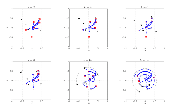
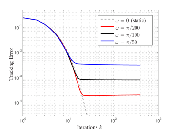
The numerical results of such setting are represented in Figures 1 and 2 for the following settings: $8$ nodes and $5$ anchors randomly deployed in the box $[-.5,0.5]^{2}$ (the maximum number of neighbors is $3$), Gaussian noise for all the measurements with the same standard deviation $\sigma=0.1$. All the nodes and anchors are moving along a circular path center in the origin with angular speed $\omega$ (different in different simulations), and the sampling period is $1$. All the decision variables of the running ADMM are initialized at $0$, and $\lambda$ is picked as $0.3$. The set $\mathcal{B}$ is taken as the whole $\mathbb{R}^{m}$ (to show that in this computational example, the choice of $\mathcal{B}$ does not influence convergence). Further details on the simulation setup are given in Simonetto2014 .

As we can see from Figures 1 and 2, the proposed running ADMM converges in primal sense and eventually reaches an error floor. The tracking error is defined as

$$\textrm{Tracking Error}(k)=\sum_{i=1}^{N}\|\mathbold{x}_{(i),k}-\mathbold{x}_{(i)}^{*}(k)\|^{2},$$ (99)

where $\mathbold{x}_{(i)}^{*}(k)$ is the centralized optimal solution at time $t_{k}$ and $\mathbold{x}_{(i),k}$ is the $k$-th iterate of the recursion (84).

We see also how the nodes are able to find and track the optimizer of a time-varying optimization problem up to a bounded error (depending on the angular speed– that is depending on the variability of the optimizers $\delta$), in a distributed fashion (i.e., by talking only to their neighbors).

Figure 1: Tracking capabilities of running ADMM with $\omega=\pi/100$. The different snapshots refer to different sampling instances $t_{k}$, $k=2,4,6,8,32,64$. The black triangles are anchor positions, the red squares are the node positions computed by an exact centralized optimization per snap-shot, the blue circles are the positions computed by the running ADMM. Lines represent the trajectories while the algorithm runs.

Figure 2: Tracking error vs. number of iterations for different angular speeds $\omega$.

Remark 1

The aim of the simulation results is to show that the theory developed in this paper can be applied to a fairly complex convex optimization problem, with semidefinite constraints, and running in a distributed fashion. More about the application example (especially in a mobile setting) can be found in Jamali-Rad2012 ; Simonetto2014a .

11 Conclusions

We have presented a general framework for time-varying optimization problems leveraging averaged operator theory. Our main meta-algorithm is the time-varying version of the fixed point algorithm, here renamed running Mann-Krasnosel’skii algorithm. With this in place, we have derived a number of convergence results for running version of commonly used algorithms in convex optimization.

Appendix: Proofs of Theorems 3.1 and  4.1

Before tackling the proof of Theorem 3.1 a technical lemma is needed.

Lemma 4

(Triangle equality, Ryu2015 ) For any scalar $\theta\in\mathbb{R}$, and vectors $\mathbold{a},\mathbold{b}\in\mathbb{R}^{n}$, the following equality holds true

$$\|(1-\theta)\mathbold{a}+\theta\mathbold{b}\|^{2}=(1-\theta)\|\mathbold{a}\|^{2}+\theta\|\mathbold{b}\|^{2}-\theta(1-\theta)\|\mathbold{a}-\mathbold{b}\|^{2}.$$ (100)

Proof

(Of Theorem 3.1)

Case (a). Starting with the basic iteration (17),

$$\|\mathbold{x}_{k+1}-\mathbold{x}\|^{2}=\|\mathsf{T}(\mathbold{x}_{k})-\mathbold{x}\|^{2}=\|\mathbold{x}_{k}+\alpha_{k}(\mathsf{G}_{k}(\mathbold{x}_{k})-\mathbold{x}_{k})-\mathbold{x}\|^{2},$$ (101)

which is true for any $k\in\mathbb{N}_{>0}$ and any $\mathbold{x}$. Let $\mathbold{x}$ be in $\mathrm{fix}\mathsf{T}_{k}=\mathrm{fix}\mathsf{G}_{k}$, i.e., $\mathbold{x}=\mathbold{x}^{*}_{k}$. Then, since by definition of fixed point $\mathbold{x}_{k}^{*}=(1-\alpha)\mathbold{x}_{k}^{*}+\alpha\mathsf{G}_{k}(\mathbold{x}^{*}_{k})$, the right-hand side can be written as

$$\|\mathbold{x}_{k+1}-\mathbold{x}^{*}_{k}\|^{2}=\|(1-\alpha_{k})(\mathbold{x}_{k}-\mathbold{x}^{*}_{k})+\alpha_{k}(\mathsf{G}_{k}(\mathbold{x}_{k})-\mathsf{G}_{k}(\mathbold{x}_{k}^{*}))\|^{2}.$$ (102)

By applying (100) and recalling that $\mathbold{x}_{k}^{*}=\mathsf{G}_{k}(\mathbold{x}^{*}_{k})$, we obtain the bound

$$\|\mathbold{x}_{k+1}-\mathbold{x}^{*}_{k}\|^{2}\leq(1-\alpha_{k})\|\mathbold{x}_{k}-\mathbold{x}^{*}_{k}\|^{2}+\\ \alpha_{k}\|\mathsf{G}_{k}(\mathbold{x}_{k})-\mathsf{G}_{k}(\mathbold{x}_{k}^{*})\|^{2}-\alpha_{k}(1-\alpha_{k})\|\mathsf{G}_{k}(\mathbold{x}_{k})-\mathbold{x}_{k}\|^{2}.$$ (103)

Since $\mathsf{G}_{k}$ is a nonexpansive operator, then $\|\mathsf{G}_{k}(\mathbold{x}_{k})-\mathsf{G}_{k}(\mathbold{x}_{k}^{*})\|^{2}\leq\|\mathbold{x}_{k}-\mathbold{x}^{*}_{k}\|^{2}$, which yields,

$$\|\mathbold{x}_{k+1}-\mathbold{x}^{*}_{k}\|^{2}\leq\|\mathbold{x}_{k}-\mathbold{x}^{*}_{k}\|^{2}-\alpha_{k}(1-\alpha_{k})\|\mathsf{G}_{k}(\mathbold{x}_{k})-\mathbold{x}_{k}\|^{2},$$ (104)

and rearranging

$$\alpha_{k}(1-\alpha_{k})\|\mathsf{G}_{k}(\mathbold{x}_{k})-\mathbold{x}_{k}\|^{2}\leq\|\mathbold{x}_{k}-\mathbold{x}^{*}_{k}\|^{2}-\|\mathbold{x}_{k+1}-\mathbold{x}^{*}_{k}\|^{2}.$$ (105)

We focus now on the term $\|\mathbold{x}_{k+1}-\mathbold{x}^{*}_{k+1}\|^{2}$. By adding and subtracting any fixed point of $\mathsf{T}_{k}$, we have

$$\|\mathbold{x}_{k+1}-\mathbold{x}^{*}_{k}-(\mathbold{x}^{*}_{k+1}-\mathbold{x}^{*}_{k})\|^{2},$$ (106)

which can be expanded as

$$\|\mathbold{x}_{k+1}-\mathbold{x}^{*}_{k}-(\mathbold{x}^{*}_{k+1}-\mathbold{x}^{*}_{k})\|^{2}=\|\mathbold{x}_{k+1}-\mathbold{x}^{*}_{k}\|^{2}+\|\mathbold{x}^{*}_{k+1}-\mathbold{x}^{*}_{k}\|^{2}\\ -2(\mathbold{x}_{k+1}-\mathbold{x}^{*}_{k})^{\mathsf{T}}(\mathbold{x}^{*}_{k+1}-\mathbold{x}^{*}_{k}),$$ (107)

and upper bounded via Assumptions 3.1-3.2 as,

$$\|\mathbold{x}_{k+1}-\mathbold{x}^{*}_{k+1}\|^{2}\leq\|\mathbold{x}_{k+1}-\mathbold{x}^{*}_{k}\|^{2}+\delta^{2}+4X\delta,$$ (108)

or equivalently

$$-\|\mathbold{x}_{k+1}-\mathbold{x}^{*}_{k}\|^{2}\leq-\|\mathbold{x}_{k+1}-\mathbold{x}^{*}_{k+1}\|^{2}+\delta^{2}+4X\delta,$$ (109)

By substituting the upper bound (109) into (105), we obtain

$$\alpha_{k}(1-\alpha_{k})\|\mathsf{G}_{k}(\mathbold{x}_{k})-\mathbold{x}_{k}\|^{2}\leq\|\mathbold{x}_{k}-\mathbold{x}^{*}_{k}\|^{2}-\|\mathbold{x}_{k+1}-\mathbold{x}^{*}_{k+1}\|^{2}+4X\delta+\delta^{2}.$$ (110)

If we now sum this inequality for all $k>0$ and discard the negative terms in the right-hand side, we obtain,

$$\sum_{k=1}^{T}\alpha_{k}(1-\alpha_{k})\|\mathsf{G}_{k}(\mathbold{x}_{k})-\mathbold{x}_{k}\|^{2}\leq\|\mathbold{x}_{1}-\mathbold{x}^{*}_{1}\|^{2}+T(4X\delta+\delta^{2}),$$ (111)

and by dividing both sides by $T$ the claim (21) follows.

Case (b) The proof in this case is straightforward. Start by,

$$\|\mathbold{x}_{k+1}-\mathbold{x}_{k+1}^{*}\| =\|\mathbold{x}_{k+1}-\mathbold{x}_{k}^{*}-(\mathbold{x}_{k}^{*}-\mathbold{x}_{k+1}^{*})\|=$$

$$=\|\mathsf{T}_{k}(\mathbold{x}_{k})-\mathsf{T}_{k}(\mathbold{x}_{k}^{*})-(\mathbold{x}_{k}^{*}-\mathbold{x}_{k+1}^{*})\|\leq L_{k}\|\mathbold{x}_{k}-\mathbold{x}_{k}^{*}\|+\delta,$$ (112)

where we have use the contractive property of $\mathsf{T}_{k}$ in Assumption 3.3, and the triangle inequality.

By iterating (Proof) backward in time, we obtain

$$\|\mathbold{x}_{k}-\mathbold{x}_{k}^{*}\|\leq L_{1}\cdots L_{k-1}\|\mathbold{x}_{1}-\mathbold{x}^{*}_{1}\|+\frac{1-\bar{L}^{k-1}_{k}}{1-\bar{L}_{k}}\delta,$$ (113)

where $\bar{L}_{k}=\max_{k}{L_{k}}$. Thus, by defining $\hat{L}_{k}=L_{1}\cdots L_{k-1}$, the claim (23) is proven. ∎

Proof

(Of Theorem 4.1)

Direct by replacing (108) by the bound (27) and following the same steps till (111). ∎

Appendix: Derivations of (84)-(85)

The derivation of the recursion (84) and (85) from the Douglas-Rachford splitting applied to the dual (83) follows from (Ryu2015, , Page 35) with minor modifications.

First of all, the update on their $y^{k}$, now reads $y^{k+1}=\Pi_{\mathcal{B}}[y^{k}+\xi^{k+1}-\zeta^{k+1}]$. With the substitutions: $\alpha\to\lambda$, $\tilde{z}^{k}\to\mathbold{z}_{k}$, $\tilde{x}^{k}\to\mathbold{x}_{k}$, and $y^{k}\to\mathbold{y}_{k}$, $\alpha u^{k}\to\mathbold{p}_{k}$, and finally $\mathbold{y}_{k}=\mathbold{p}_{k}+\lambda(\mathbold{A}\mathbold{x}_{k+1}-\mathbold{c})$, then (84) follows directly. Note that one cannot swap the order of $\mathbold{p}_{k+1}$ and $\mathbold{x}_{k+1}$ to obtain the standard ADMM, since now $\mathbold{p}_{k+1}$ depends on both $\mathbold{x}_{k}$ and $\mathbold{x}_{k+1}$. To obtain the dual variable $\mathbold{\nu}_{k+1}$, as for the Douglas-Rachford splitting (76) we have that is equivalent to their $\zeta^{k+1}$, that is

$$\mathbold{\nu}_{k+1}=\mathbold{y}^{k}+\lambda\mathbold{B}\mathbold{z}_{k+1}=\mathbold{p}_{k}+\lambda(\mathbold{A}\mathbold{x}_{k+1}+\mathbold{B}\mathbold{z}_{k+1}-\mathbold{c}),$$ (114)

from which the relation after (84) follows.

When $\mathcal{B}=\mathbb{R}^{m}$, then the steps of (Ryu2015, , Page 35) can be carried out till the end and the standard ADMM follows. In particular, due to (114), $\mathbold{\nu}_{k+1}=\mathbold{p}_{k+1}$.

References

- (1) Jerez, J.L., Goulart, P.J., Richter, S., Constantinides, G.A., Kerrigan, E.C., Morari, M.: Embedded Online Optimization for Model Predictive Control at Megahertz Rates. IEEE Transactions on Automatic Control 59(12), 3238 – 3251 (2014)
- (2) Hours, J.H., Jones, C.N.: A Parametric Non-Convex Decomposition Algorithm for Real-Time and Distributed NMPC. IEEE Transactions on Automatic Control 61(2), 287 – 302 (2016)
- (3) Gutjahr, B., Gröll, L., Werling, M.: Lateral Vehicle Trajectory Optimization Using Constrained Linear Time-Varying MPC. IEEE Transactions on Intelligent Transportation Systems PP(99), 1 – 10 (2016)
- (4) Jakubiec, F.Y., Ribeiro, A.: D-MAP: Distributed Maximum a Posteriori Probability Estimation of Dynamic Systems. IEEE Transactions on Signal Processing 61(2), 450 – 466 (2013)
- (5) Asif, M.S., Romberg, J.: Sparse recovery of streaming signals using -homotopy . IEEE Transactions on Signal Processing 62(16), 4209 – 4223 (2014)
- (6) Yang, Y., Zhang, M., Pesavento, M., Palomar, D.P.: An Online Parallel and Distributed Algorithm for Recursive Estimation of Sparse Signals. IEEE Transactions on Signal and Information Processing over Networks 2(3), 290 – 305 (2016)
- (7) Vaswani, N., Zhan, J.: Recursive Recovery of Sparse Signal Sequences from Compressive Measurements: A Review. IEEE Transactions on Signal Processing 64(13), 3523 – 3549 (2016)
- (8) Balavoine, A., Romberg, J., Rozell, C.: Discrete and continuous iterative soft thresholding with a dynamic input. IEEE Transactions on Signal Processing 63(12), 3165 – 3176 (2015)
- (9) Simonetto, A., Leus, G.: On Non-Differentiable Time-Varying Optimization. In: Proceedings of the 6th IEEE International Workshop on Computational Advances in Multi-Sensor Adaptive Processing. Cancun, Mexico (2015)
- (10) Sopasakis, P., Freris, N., Patrinos, P.: Accelerated Reconstruction of a Compressively Sampled Data Stream. In: Proceedings of the 24th European Signal Processing Conference, pp. 1078 – 1082. Budapest, Hungary (2016)
- (11) Baingana, B., Traganitis, P., Mateos, G., Giannakis, G.B.: Big Data Analytics for Social Networks, in Graph Analysis for Social Media. CRC Press (2015)
- (12) Ardeshiri, T., Norrlöf, M., Löfberg, J., Hansson, A.: Convex Optimization Approach for Time-Optimal Path Tracking of Robots with Speed Dependent Constraints. In: Proceedings of the 18th IFAC World Congress, pp. 14,648 – 14,653. Milano, Italy (2011)
- (13) Verscheure, D., Demeulenaere, B., Swevers, J., De Schutter, J., Diehl, M.: Time-Optimal Path Tracking for Robots: a Convex Optimization Approach. IEEE Transactions on Automatic Control 54(10), 2318 – 2327 (2009)
- (14) Koppel, A., Warnell, G., Stumpe, E., Ribeiro, A.: D4L: Decentralized Dynamic Discriminative Dictionary Learning. IEEE Transactions Signal and Information Processing over Networks (submitted) (2016)
- (15) Zhao, C., Topcu, U., Li, N., Low, S.: Design and Stability of Load-Side Primary Frequency Control in Power Systems. IEEE Transactions on Automatic Control (2014). To appear
- (16) Dall’Anese, E., Simonetto, A.: Optimal Power Flow Pursuit. IEEE Transactions on Smart Grid, in press (2016)
- (17) Dontchev, A.L., Krastanov, M.I., Rockafellar, R.T., Veliov, V.M.: An Euler-Newton Continuation method for Tracking Solution Trajectories of Parametric Variational Inequalities. SIAM Journal of Control and Optimization 51(51), 1823 – 1840 (2013)
- (18) Uecker, M., Zhang, S., Voit, D., Merboldt, K.D., Frahm, J.: Real-time MRI: recent advances using radial FLASH. Imaging Medicine 4(4), 461 – 476 (2012)
- (19) Popkov, A.Y.: Gradient Methods for Nonstationary Unconstrained Optimization Problems. Automation and Remote Control 66(6), 883 – 891 (2005). Translated from Avtomatika i Telemekhanika, No. 6, 2005, pp. 38 – 46
- (20) Tu, S.Y., Sayed, A.H.: Mobile Adaptive Networks. IEEE Journal of Selected Topics in Signal Processing 5(4), 649 – 664 (2011)
- (21) Bajovic, D., Jakovetic, D., Xavier, J., Sinopoli, B., Moura, J.M.F.: Distributed Detection via Gaussian Running Consensus: Large Deviations Asymptotic Analysis. IEEE Transactions on Signal Processing 59(9), 4381 – 4396 (2011)
- (22) Zavlanos, M.M., Ribeiro, A., Pappas, G.J.: Network Integrity in Mobile Robotic Networks. IEEE Transactions on Automatic Control 58(1), 3 – 18 (2013)
- (23) Ling, Q., Ribeiro, A.: Decentralized Dynamic Optimization Through the Alternating Direction Method of Multipliers. IEEE Transactions on Signal Processing 62(5), 1185 – 1197 (2014)
- (24) Simonetto, A., Leus, G.: Distributed Asynchronous Time-Varying Constrained Optimization. In: Proceedings of the Asilomar Conference on Signals, Systems, and Computers. Pacific Grove, USA (2014)
- (25) Simonetto, A., Leus, G.: Double Smoothing for Time-Varying Distributed Multi-user Optimization. In: Proceedings of the IEEE Global Conference on Signal and Information Processing. Atlanta, US (2014)
- (26) Ye, M., Hu, G.: Distributed Optimization for Systems with Time-Varying Quadratic Objective Functions. In: Proceedings of the 54th IEEE Conference on Decision and Control, pp. 3285 – 3290. Osaka, Japan (2015)
- (27) Xi, C., Khan, U.A.: Distributed Dynamic Optimization over Directed Graphs. In: Proceedings of the 55th IEEE Conference on Decision and Control, pp. 245 – 250. Las Vegas, NV, US (2016)
- (28) Sun, C., Ye, M., Hu, G.: Distributed Time-varying Quadratic Optimization for Multiple Agents under Undirected Graphs. IEEE Transactions on Automatic Control (to appear) (2017)
- (29) Maros, M., Jalden, J.: ADMM for Distributed Dynamic Beam-forming. IEEE Transactions on Signal and Information Processing over Networks (to appear) (2017)
- (30) Simonetto, A., Mokhtari, A., Koppel, A., Leus, G., Ribeiro, A.: A Class of Prediction-Correction Methods for Time-Varying Convex Optimization. IEEE Transactions on Signal Processing 64(17), 4576 – 4591 (2016)
- (31) Simonetto, A., Koppel, A., Mokhtari, A., Leus, G., Ribeiro, A.: Decentralized Prediction-Correction Methods for Networked Time-Varying Convex Optimization. IEEE Transactions on Automatic Control (to appear) (2017)
- (32) Simonetto, A., Dall’Anese, E.: Prediction-Correction Algorithms for Time-Varying Constrained Optimization. IEEE Transactions on Signal Processing 65(20), 5481 – 5494 (2017)
- (33) Rahili, S., Ren, W.: Distributed Convex Optimization for Continuous-Time Dynamics with Time-Varying Cost Functions. IEEE Transactions on Automatic Control (to appear) (2016)
- (34) Fazlyab, M., Paternain, S., Preciado, V., Ribeiro, A.: Interior Point Method for Dynamic Constrained Optimization in Continuous Time. In: Proceedings of the American Control Conference, pp. 5612 – 5618. Boston (MA), USA (2016)
- (35) Fazlyab, M., Paternain, S., Preciado, V., Ribeiro, A.: Prediction-Correction Interior-Point Method for Time-Varying Convex Optimization. arXiv: 1608.07544 (2016)
- (36) Bauschke, H.H., Combettes, P.L.: Convex Analysis and Monotone Operator Theory in Hilbert Spaces. CMS Books in Mathematics. Springer-Verlag (2011)
- (37) Ryu, E.K., Boyd, S.: Primer on Monotone Operator Methods. Applied Computational Mathematics 15(1), 3 – 43 (2016)
- (38) Rockafellar, R.: Convex Analysis. Princeton University Press, New Jersey (1970)
- (39) Eckstein, J.: Splitting Methods for Monotone Operators with Applications to Parallel Optimization. Ph.D. thesis, MIT (1989)
- (40) Rockafellar, R.T., Wets, R.J.B.: Variational Analysis. Springer (1998)
- (41) Aragón Artacho, F.J., Borwein, J.M., Martín-Márquez, V., Yao, L.: Applications of convex analysis within mathematics. Mathematical Programming 148(1 – 2), 49 – 88 (2014)
- (42) Combettes, P., Tamada, I.: Compositions and Convex Combinations of Averaged Nonexpansive Operators. Journal of Mathematical Analysis and Applications 425(1), 55 – 70 (2015)
- (43) Cominetti, R., Soto, J., Vaisman, J.: On the rate of convergence of Krasnosel’skiı-Mann iterations and their connection with sums of Bernoullis. Israel Journal of Mathematics 199, 757 – 772 (2014)
- (44) Vaisman, J.: Convergencia fuerte del metodo de medias sucesivas para operadores lineales no-expansivos. Tech. rep., Memoria de Ingenieria Civil Matematica, Universidad de Chile (2005)
- (45) Goldstein, A.: Convex Programming in Hilbert Space. Bulletin of the American Mathematical Society 70(5), 709 – 710 (1964)
- (46) Levitin, E., Polyak, B.: Constrained Minimization Methods. Zhurnal Vychislitel’noi Matematiki i Matematicheskoi Fiziki 6(5), 787 – 823 (1966)
- (47) Rockafellar, R.T.: Monotone Operators and the Proximal Point Algorithm. SIAM Journal of Control and Optimization 14(5), 877 – 898 (1976)
- (48) Beck, A., Teboulle, M.: A Fast Iterative Shrinkage-Thresholding Algorithm for Linear Inverse Problems. SIAM Journal on Imaging Sciences 2(1), 183 – 202 (2009)
- (49) Tseng, P.: Dual Ascent Methods for Problems with Strictly Convex Costs and Linear Constraints: A Unified Approach. SIAM Journal on Control and Optimization 28(1), 214 – 242 (1990)
- (50) Nedić, A., Ozdaglar, A.: Approximate Primal Solutions and Rate Analysis for Dual Subgradient Methods. SIAM Journal on Optimization 19(4), 1757 – 1780 (2009)
- (51) Combettes, P., Wajs, V.: Signal Recovery by Proximal Forward-Backward Splitting. Multiscale Modeling and Simulation 4(4), 1168 – 1200 (2005)
- (52) Duchi, J., Singer, Y.: Efficient Online and Batch Learning Using Forward Backward Splitting. Journal of Machine Learning Research 10, 2899 – 2934 (2009)
- (53) Bertsekas, D.P., Tsitsiklis, J.N.: Parallel and Distributed Computation: Numerical Methods. Athena Scientific, Belmont, Massachusetts (1997)
- (54) Schizas, I.D., Ribeiro, A., Giannakis, G.B.: Consensus in Ad Hoc WSNs With Noisy Links— Part I: Distributed Estimation of Deterministic Signals. IEEE Transactions on Signal Processing 56(1), 350 – 364 (2008)
- (55) Boyd, S., Parikh, N., Chu, E., Peleato, B., Eckstein, J.: Distributed Optimization and Statistical Learning via the Alternating Direction Method of Multipliers. Foundations and Trends® in Machine Learning 3(1), 1 – 122 (2011)
- (56) Johansson, B., Keviczky, T., Johansson, M., Johansson, K.H.: Subgradient Methods and Consensus Algorithms for Solving Convex Optimization Problems. In: Proceedings of the 47th IEEE Conference on Decision and Control, pp. 4185 – 4190. Cancun, Mexico (2008)
- (57) Koshal, J., Nedić, A., Shanbhag, U.Y.: Multiuser Optimization: Distributed Algorithms and Error Analysis. SIAM Journal on Optimization 21(3), 1046 – 1081 (2011)
- (58) Koppel, A., Jakubiec, F.Y., Ribeiro, A.: A Saddle Point Algorithm for Networked Online Convex Optimization. IEEE Transactions on Signal Processing 63(19), 5149 – 5164 (2015)
- (59) Shalev-Shwartz, S.: Online Learning and Online Convex Optimization. Foundations and Trends® in Machine Learning 4(2), 107 – 194 (2012)
- (60) Combettes, P., Pennanen, T.: Generalized Mann Iterates for Constructing Fixed Points in Hilbert Spaces. Journal of Mathematical Analysis and Applications 275(2), 521 – 536 (2002)
- (61) Davis, D., Yin, W.: Convergence Rate Analysis of Several Splitting Schemes. In: R. Glowinski and S. Osher and W. Yin (Ed.s), Splitting Methods in Communication and Imaging, Science and Engineering, Springer (to appear)
- (62) Frankel, P., Garrigos, G., Peypouquet, J.: Splitting Methods with Variable Metric for Kurdyka-Lojasiewicz Functions and General Convergence Rates. Journal of Optimization Theory and Applications 165, 874 – 900 (2015)
- (63) Bianchi, P.: Ergodic convergence of a stochastic proximal point algorithm. SIAM Journal on Optimization 26(4), 2235 – 2260 (2016)
- (64) Garrigos, G., Rosasco, L., Villa, S.: Convergence of the Forward-Backward Algorithm: Beyond the Worst Case with the Help of Geometry. arXiv: 1703.09477 (2017)
- (65) Bauschke, H., Noll, D., Phan, H.: Linear and Strong Convergence of Algorithms Involving Averaged Nonexpansive Operators. Journal of Mathematical Analysis and Applications 421(1), 1 – 20 (2015)
- (66) Banjac, G., Goulart, P.: Tight Global Linear Convergence Rate Bounds for Operator Splitting Methods. Preprint (2016)
- (67) Necoara, I., Yu. Nesterov, Glineur, F.: Linear Convergence of First Order Methods for Non-Strongly Convex Optimization. Preprint (2015)
- (68) Borwein, J., Li, G., Tam, M.: Convergence Rate Analysis for Averaged Fixed Point Iterations in the Presence of Hölder Regularity. Preprint (2015)
- (69) Themelis, A., Patrinos, P.: SuperMann: a superlinearly convergent algorithm for finding fixed points of nonexpansive operators. arXiv:1609.06955 (2016)
- (70) Bravo, M., Cominetti, R.: Sharp convergence rates for averaged nonexpansive maps. arXiv: 1606.05300 (2016)
- (71) Bravo, M., Cominetti, R., Pavez-Singé, M.: Rates of convergence for inexact Krasnosel’skii-Mann iterations in Banach spaces. arXiv:1705.09340v2 (2017)
- (72) Zhao, J., Yang, Q.: Several solution methods for the split feasibility problem. Inverse Problem 21, 1791 (2005)
- (73) Xu, H.: A variable Krasnosel’skii-Mann algorithm and the multiple-set split feasibility problem. Inverse Problem 22, 2021 – 2034 (2006)
- (74) Peypouquet, J.: Asymptotic convergence to the optimal value of diagonal proximal iterations in convex minimization. Journal of Convex Analysis 16, 277 – 286 (2009)
- (75) Peypouquet, J., Sorin, S.: Evolution equations for maximal monotone operators: asymptotic analysis in continuous and discrete time. Journal of Convex Analysis 17, 1113 – 1163 (2010)
- (76) Moreau, J.J.: Evolution Problem Associated with a Moving Convex Set in a Hilbert Space. Journal of Differential Equations 26, 347 – 374 (1977)
- (77) Briceno-Arias, L.M., Hoang, N.D., Peypouquet, J.: Existence, stability and optimality for optimal control problems governed by maximal monotone operators. Journal of Differential Equations 260, 733 – 757 (2016)
- (78) Dontchev, A., Lempio, F.: Difference methods for differential inclusions: A survey. SIAM Review 34(2), 263 – 294 (1992)
- (79) Cojocaru, M.G., Daniele, P., Nagurney, A.: Projected Dynamical Systems and Evolutionary Variational Inequalities via Hilbert Spaces with Applications. Journal of Optimization Theory and Applications 127(3), 549 – 563 (2005)
- (80) Nagurney, A., Pan, J.: Evolution Variational Inequalities and Projected Dynamical Systems with Application to Human Migration. Mathematical and Computer Modelling 43(5 – 6), 646 – 657 (2006)
- (81) Taylor, A.: Convex Interpolation and Performance Estimation of First-order Methods for Convex Optimization. Ph.D. thesis, Université catholique Louvain, Belgium (2017)
- (82) Dontchev, A.L., Rockafellar, R.T.: Implicit Functions and Solution Mappings. Springer (2009)
- (83) Erseghe, T.: A Distributed and Maximum-Likelihood Sensor Network Localization Algorithm Based Upon a Nonconvex Problem Formulation. IEEE Transactions on Signal and Information Processing over Networks 1(4), 247 – 258 (2015)
- (84) Giselsson, P., Boyd, S.: Linear Convergence and Metric Selection for Douglas-Rachford Splitting and ADMM. to appear in IEEE Transactions on Automatic Control (2017)
- (85) Simonetto, A., Leus, G.: Distributed Maximum Likelihood Sensor Network Localization. IEEE Transactions on Signal Processing 62(6), 1424 – 1437 (2014)
- (86) Jamali-Rad, H., Leus, G.: Dynamic Multidimensional Scaling for Low-Complexity Mobile Network Tracking. IEEE Transactions on Signal Processing 60(8), 4485 – 4491 (2012)
- (87) Simonetto, A., Leus, G.: A Moving Horizon Convex Relaxation for Mobile Sensor Network Localization. In: Proceeding of the 8th IEEE Sensor Array and Multichannel Signal Processing Workshop. La Coruna, Spain (2014)