Doubled Khovanov Homology
Abstract.
We define a homology theory of virtual links built out of the direct sum of the standard Khovanov complex with itself, motivating the name doubled Khovanov homology. We demonstrate that it can be used to show that some virtual links are non-classical, and that it yields a condition on a virtual knot being the connect sum of two unknots. Further, we show that doubled Khovanov homology possesses a perturbation analogous to that defined by Lee in the classical case and define a doubled Rasmussen invariant. This invariant is used to obtain various cobordism obstructions; in particular it is an obstruction to sliceness. Finally, we show that the doubled Rasmussen invariant contains the odd writhe of a virtual knot, and use this to show that knots with non-zero odd writhe are not slice.
Key words and phrases:
Khovanov homology, virtual knot concordance, virtual knot theory1991 Mathematics Subject Classification:
57M25, 57M27, 57N701. Introduction
1.1. Statement of results
This paper defines and investigates the properties of a homology theory of virtual links, the titular doubled Khovanov homology. For a virtual link we denote by its doubled Khovanov homology, a bigraded finitely generated Abelian group. Below are two examples of the doubled Khovanov homologies of links, split horizontally by the first (homological) grading and vertically by second (quantum) grading; for more detail see Figures 6 and 7. The position of indicates in the quantum grading, and the right-hand column of the first pair of grids is at homological degree :
Also depicted is the homology of virtual links first defined by Manturov [15] and reformulated by Dye, Kaestner, and Kauffman [5], denoted by . One observes that, while the groups assigned to the links by each theory are not disjoint, they differ substantially. Specifically, we see that and both contain a term for each component of the argument, and that also contains the knight’s move familiar from classical Khovanov homology [1]. In contrast contains a knight’s move and a term, whereas contains only a single knight’s move.
Doubled Khovanov homology can sometimes detect non-classicality of a virtual link.
Theorem (Corollary 2.5 of Section 2.2).
Let be a virtual link. If
for a non-trivial bigraded Abelian group, then is non-classical.
The graded Euler characteristic of the theory contains no new information.
Theorem.
Let be a virtual link. Denote by the graded Euler characteristic of with respect to the quantum grading. Then , for the Jones polynomial of .
The connect sum operation on virtual knots exhibits more complicated behaviour than that of the classical case: the result of a connect sum between two virtual knots depends on both the diagrams used and the site at which the connect sum is conducted. Indeed, there are multiple inequivalent virtual knots which can be obtained as connect sums of a fixed pair of virtual knots. A surprising consequence of this that there are non-trivial virtual knots which can be obtained as a connect sum of a pair of unknots. Doubled Khovanov homology yields a condition met by such knots.
Theorem (Theorem 5.12 of Section 5.2).
Let be a virtual knot which is a connect sum of two trivial knots. Then .
Further, there is a perturbation of doubled Khovanov homology akin to Lee’s perturbation of Khovanov homology; we denote it by and refer to it as doubled Lee homology. Unlike the classical case, however, doubled Lee homology vanishes for certain links. We show this in two steps. Firstly, we prove that the rank of doubled Lee homology behaves analogously to that of classical Lee homology.
Theorem (Theorem 3.5 of Section 3.1).
Given a virtual link
Secondly, in Theorem 3.12 of Section 3.1, we determine the number of alternately coloured smoothings of a virtual link. In abbreviated form, Theorem 3.12 states that a virtual link has either or alternately coloured smoothings, and that one can determine which case holds via a simple check on a (Gauss diagram of a) diagram of . This explains why is a single knight’s move: a knight’s move cancels when we pass to doubled Lee homology and ![]() has no alternately coloured smoothings.
has no alternately coloured smoothings.
Kauffman related alternately coloured smoothings of virtual link diagrams to perfect matchings of -valent graphs [8], and using that correspondence we observe that doubled Lee homology yields the following equivalent to the Four Colour Theorem. (A graph is bridgeless if it does not possess an edge the removal of which increases the number of connected components of the graph.)
Theorem.
Let be a planar, bridgeless, -valent graph and a perfect matching of . Associated to the pair is a family of virtual link diagrams. Denote a member of this family by . Then there exists a perfect matching such that
for all .
Doubled Lee homology cannot vanish for virtual knots, however; we show that a virtual knot has exactly alternately coloured smoothings, so that its homology is of rank . In Section 4 we show that the information contained in is equivalent to a pair of integers, denoted , and referred to as the doubled Rasmussen invariant; contains information regarding the quantum grading, the homological grading. Using we are able to give the following obstructions to the existence of various kinds of cobordisms.
Theorem (Theorem 5.3 of Section 5.1.1).
Let and be a pair of virtual knots with , and be a certain type of cobordism from between them such that every link appearing in has a generator in homological degree . Then
Theorem (Theorem 5.6 of Section 5.1.2).
Let be a virtual link of components. Further, let be a connected concordance between and a virtual knot such that . Let be the maximum non-trivial quantum degree of elements such that . Then
Both components of the doubled Rasmussen invariant are concordance invariants and obstructions to sliceness; in Sections 3.2 and 5.1 we use the functorial nature of doubled Lee homology to show this. In addition, the homological degree information contained in the invariant is equivalent to the odd writhe, so that we are able to show that this well known invariant is also an obstruction to sliceness.
Theorem (Proposition 4.11 of Section 4.3).
Let be a virtual knot. Then , where is the odd writhe of .
Theorem (Theorem 5.8 of Section 5.1.3).
Let be a virtual knot and its odd writhe. If then is not slice.
Theorem (Theorem 5.4 of Section 5.1.1).
Let and be virtual knots such that . If then and are not concordant.
Finally, using the above results, we show that there exist virtual knots which are not concordant to any classical knots.
Theorem (Corollary 5.10 of Section 5.1.3).
Let be a virtual knot. If then is not concordant to a classical knot.
1.2. Extending Khovanov homology
The first successful extension of Khovanov homology to virtual links was produced by Manturov [15], as mentioned above. His work was reformulated by Dye, Kaestner, and Kauffman in order to define a virtual Rasmussen invariant [5]. Tubbenhauer has also developed a virtual Khovanov homology using non-orientable cobordisms [22]. Doubled Khovanov homology is as an alternative extension of Khovanov homology to virtual links.
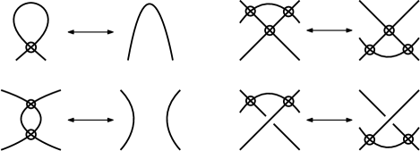
Any extension of Khovanov homology to virtual links must deal with the fundamental problem presented by the single cycle smoothing, also known as the one-to-one bifurcation. This is depicted in Figure 1: altering the resolution of a crossing no longer either splits one cycle or merges two cycles, but can in fact take one cycle to one cycle. The realisation of this as a cobordism between smoothings is a once-punctured Möbius band. How does one associate an algebraic map, , to this? Looking at the quantum grading (where the module associated to one cycle is ) we notice that
from which we observe that the map must be the zero map if it is to be grading-preserving (we have arranged the generators vertically by quantum grading). This is the approach taken by Manturov and subsequently Dye et al.
Another way to solve this problem is to “double up” the complex associated to a link diagram in order to plug the gaps in the quantum grading, so that the map may be non-zero. The notion of “doubling up” will be made precise in Section 2, but for now let us look at the example of the single cycle smoothing: if we take the direct sum of the standard Khovanov chain complex with itself, but shifted in quantum grading by , we obtain , that is
where and (u for “upper” and l for “lower”) are graded modules and for a graded module . Thus the map associated to the single cycle smoothing may now be non-zero while still degree-preserving. It is this approach which we take in the following work.
1.3. Plan of the paper
In Section 2 we define the doubled Khovanov homology theory and describe some of its properties: we find the doubled Khovanov homology of classical links, and illustrate a method to produce an infinite number of non-trivial virtual knots with doubled Khovanov homology of the unknot. In Section 3 we define a perturbation analogous to Lee homology of classical links and show that, as in the classical case, the rank of this perturbed theory can be computed in terms of alternately coloured smoothings. We then investigate the functorial nature of the perturbed theory. Section 4 contains the definition of the doubled Rasmussen invariant and a description of its properties. Finally, in Section 5 the invariants are put to use, yielding topological applications.
We assume familiarity with classical Khovanov homology and the rudiments of virtual knot theory.
2. Doubled Khovanov homology
2.1. Definition
In the tradition of classical Khovanov homology and its descendants doubled Khovanov homology assigns to an oriented virtual link diagram a bigraded Abelian group which is the homology of a chain complex; the result is an invariant of the link represented. In contrast to other virtual extensions of Khovanov homology, however, the work of dealing with the single cycle smoothing (see Figure 1) is done in the realm of algebra so that certain verifications require no new technology to complete (c.f. with the order construction used in [5]).
Definition 2.1 (Doubled Khovanov complex).
Let be an oriented virtual link diagram with positive classical crossings and negative classical crossings. Form the cube of smoothings associated to in the standard manner by resolving classical crossings and leaving virtual crossings unchanged – see the example given in Figure 2.
Let (under the identification , ) where is either or . Form a chain complex by associating to a smoothing consisting of cycles (that is, copies of immersed in the plane) a vector space in the following way
| (2.1) |
We refer to the unshifted (shifted) summand as the upper (lower) summand and denote elements in the upper summand by a superscript u and those in the lower summand by a superscript l. We also suppress tensor products, concatenating them into one subscript e.g.
or
The components of the differential are built in the standard way as matrices with entries the maps , , and , whose positions are read off from the cube of smoothings. The and maps are given by
| (2.2) | ||||||
(so that they do not map between the upper and lower summands). The map associated to the single cycle smoothing as in Figure 1 is given by
| (2.3) | ||||||
The effect of the map on tensor products is (possibly) to alter the superscript of entire string and the subscript of the tensorand in question. For example, if the cycle undergoing the single cycle smoothing is corresponds to the second tensor factor
Any assignment of signs to the maps within the cube of smoothings which yields anticommutative faces produces isomorphic chain complexes.
Let denote the direct sum of the vector spaces assigned to the smoothings with exactly -resolutions. Define the chain spaces of the doubled Khovanov complex to be
| (2.4) |
(where denotes a shift in homological degree). An example of such a chain complex is given in Figure 3.
Remark.
The map given in Equation 2.3 is not an -module map, so that is not an extended Frobenius algebra in the sense of [23], and doubled Khovanov homology seemingly cannot be interpreted as an unoriented topological field theory. (Also, doubled Lee homology, as defined in Section 3, does not satisfy the multiplicativity axiom of an unoriented topological field theory.)
Proposition 2.2.
Equipped with the differential given by matrices of maps as described in Definition 2.1 is a chain complex.
Proof.
It is enough to verify the commutativity of the faces
as the face
cannot occur. We leave the algebra to the reader and note that, as in the classical case, sprinkling signs appropriately yields a chain complex. ∎
Theorem 2.3.
Given an oriented virtual link diagram the chain homotopy equivalence class of is an invariant of the oriented link represented by . The homology of , denoted , is therefore also an invariant of the link represented by .
Proof.
We are required to construct chain homotopy equivalences for each of the virtual Reidemeister moves. It is readily observed that if two diagrams and are related by a finite sequence of the purely virtual moves and mixed move (depicted in Figure 4) then as these moves do not alter the number of cycles in a smoothing nor the incoming and outcoming maps.
2.2. Detection of non-classicality
We say that a virtual link is non-classical if all diagrams representing it have at least one virtual crossing. Conversely, we say that a virtual link is classical if it has a diagram with no virtual crossings. Doubled Khovanov homology can sometimes be used to detect non-classicality.
Consider the complex associated to the classical diagram of the unknot given in Figure 5: the reader notices immediately that not only do the chain spaces decompose as direct sums, the entire complex does also (as there are no maps). That is
| (2.5) |
where denotes the classical Khovanov complex of a diagram . This motivates the following proposition.
Proposition 2.4.
Let be a virtual link. If is classical then there exists a diagram of , denoted , which has no classical crossings. Then
where denotes the standard Khovanov homology of a classical link.
Proof.
This is an obvious consequence of Equation 2.5, which holds for all classical diagrams. ∎
The contrapositive statement to that of Proposition 2.4 is:
Corollary 2.5.
Let be a virtual link. If
| (2.6) |
for a non-trivial bigraded Abelian group, then is non-classical.
As an example consider the virtual knot in Green’s table [6], depicted in Figure 6, along with its doubled Khovanov homology, split by homological grading (horizontal axis) and quantum grading (vertical axis).
Another interesting example is given by the so-called virtual Hopf link, given in Figure 7; we shall look into it further in Section 3.
The statement within Corollary 2.5 cannot be upgraded to an equivalence, however. A counterexample is given by the virtual knot in Green’s table, depicted on the right of Figure 8 (the non-classicality of is demonstrated by its generalised Alexander polynomial [10]). The cube of smoothings associated to does not contain any maps, and therefore for some non-trivial Abelian group . In fact, . This follows from the fact that can be obtained from a diagram of the unknot by applying the following move on diagrams
Definition 2.6.
Within an oriented virtual link diagram one may place a virtual crossing on either side of a classical crossing in the following manner
This move is known as flanking.
Flanking is also known virtualization, but as there is some confusion in the literature regarding that term we avoid it.
Proposition 2.7.
If a virtual link diagram can be obtained from another, , by a flanking move then .
Proof.
Let and be as in the proposition. Consider the tangle diagrams by produced by isolating a neighbourhood of the classical crossing undergoing the flanking move in and a neighbourhood of the result of the flanking move in . We construct an identification of the smoothings of with those of using the smoothings of the tangle diagrams depicted in Figure 9: a smoothing of must contain either or , and we associate to it the smoothing of formed by replacing with , or with . One readily sees that this identification is a bijection which does not change the number of cycles in a smoothing nor how those cycles are linked. Thus the chain spaces of and are equal, and so are the components of the differential. ∎
Corollary 2.8.
There is an infinite number of non-trivial virtual knots with doubled Khovanov homology equal to that of the unknot.
3. Doubled Lee homology
In Section 3.1 we define doubled Lee homology and prove some of its properties, and in Section 3.2 we investigate aspects of the functorial nature of the theory.
3.1. Definition
The reader may have noticed that there are generators of the homologies depicted in Figure 6 and Figure 7 which are apart in quantum degree. Quantum degree separations of length are important in classical Khovanov homology; Lee’s perturbation of Khovanov homology [14] is defined by adding to the differential a component of degree . Such a perturbation of doubled Khovanov homology exists also.
Definition 3.1 (Doubled Lee homology).
Let be an oriented virtual link diagram and denote the chain complex with the chain spaces of but with altered differential, and . The components of this differential are as follows
and
The above maps are no longer graded, but filtered (as in the classical case). That is a chain complex is verified as in Proposition 2.2. Setting to be the homology of , define the doubled Lee homology of
where is the link represented by .
Theorem 3.2.
For a virtual link diagram , is an invariant of the link represented by .
As in the classical case, doubled Khovanov homology and doubled Lee homology are related in the following manner.
Theorem 3.3.
For any virtual link there is a spectral sequence with page converging to .
The rank of the classical Lee homology of a link depends only on the number of its components. Precisely, for a classical link
| (3.1) |
where denotes the number of components of and its classical Lee homology. In fact, Equation 3.1 follows from the following two statements [3]:
| (3.2) |
and
| (3.3) |
given the following definition:
Definition 3.4.
A smoothing of a virtual link diagram is alternately coloured if its cycles are coloured exactly one of two colours in such a way that in a neighbourhood of each classical crossing the two incident arcs are different colours. A smoothing which can be coloured in such a way is known as an alternately colourable.
(Any potential issue raised by the fact that Definition 3.4 regards diagrams while Equations 3.2 and 3.3 are statements about links is resolved by Theorem 3.5, which shows that the number of alternately coloured smoothings is a link invariant.)
In the virtual case we recover Equation 3.2 (up to a scalar) but not Equation 3.3.
Theorem 3.5.
Given a virtual link
We postpone stating the virtual generalisation of Equation 3.3 until we have proved Theorem 3.5, for which we require the following analogue of a classical result.
Lemma 3.6.
Let be a diagram of a virtual link . There is an action of on which descends to an action on .
Proof.
Given a virtual link diagram define an action of on in the following manner: mark a point on and maintain it across the smoothings of . The action is given by
where the -th cycle is marked (component-wise multiplication is given by ). Clearly this action endows with the structure of an -module. To show that is also an -module it suffices to show that the action defined above commutes with the differential. We verify this in the case of and multiplication by , with the marked point on the cycle corresponding to the first tensor factor:
as required. The other cases are left to the reader. ∎
Further, we define a new basis for : the familiar “red” and “green” basis first given by Bar-Natan and Morrison.
Definition 3.7.
Let be the basis for where
| “red” | |||
| “green” |
We denote the corresponding generators of as , , , and .
We denote which generator a cycle of a smoothing is labelled with by colouring that cycle either red or green. Thus alternately coloured smoothings are such that given any two cycles which share a crossing (i.e. they pass through the same crossing neighbourhood) one is coloured red and the other green.
We shall use the following definition in the remainder of this work.
Definition 3.8.
Let be an oriented virtual link diagram with negative classical crossings, and an alternately coloured smoothing in which classical crossings (positive or negative) resolved into their -resolution. Define the height of to be . Of course, if are the alternately coloured generators assigned to then .
Proof of Theorem 3.5.
Let be a diagram of and be an alternately coloured smoothing of , with cycles coloured either red or green, and be the algebraic element given by
| (3.4) |
where
and likewise define , so that to each alternately coloured smoothing we associate two algebraic objects. We refer to such ’s as alternately coloured generators, a term we justify with the following steps: we shall show that such elements are homologically non-trivial and distinct, and that they do indeed generate .
First notice that alternately coloured smoothings have restricted incoming and outgoing differentials: if a smoothing has an map either incoming or outgoing then it must have a crossing neighbourhood with only one cycle passing through it. Such a crossing neighbourhood cannot satisfy the alternately coloured condition. Likewise, if a smoothing has an incoming map or an outgoing map it must have a crossing neighbourhood with only one cycle passing through. Thus an alternately coloured smoothing has only incoming maps and outgoing maps and homological non-triviality of the associated is equivalent to and . With respect to the basis we have
| (3.5) | ||||||
so that clearly .
Let and be two alternately coloured smoothings of and , their associated alternately coloured generators. Notice that it is possible that and are alternately coloured smoothings associated to the same uncoloured smoothing of . We shall consider the two cases: and are not alternately coloured smoothings associated to the same uncoloured smoothing of and they are.
: It is possible that and are at different height (that is, they have a different number of -resolutions). Then as they are of differing homological grading. If and are at the same height, , say, we recall that is a direct sum of the modules associated to all smoothings of height so that can be written
so that .
: Mark a point on such that the cycles of and on which the point lies are opposite colours (such a point always exists as ), and define the action of as in Lemma 3.6. Notice that and so that
as if the marked cycle is red in then it is green in and vice versa. As the action descends to an action on we see that is an eigenvector of the action of of eigenvalue and is an eigenvector of eigenvalue , so that .
At this point we have
In order to tighten this to an equality we shall again employ Gauss elimination along with the observation that the differential restricted to elements corresponding to non-alternately coloured smoothings is an isomorphism. In the case of the and maps this is evident from Equation 3.5. Regarding the map, we have
| (3.6) | ||||||
so that is an isomorphism (we are working over ). Thus we Gauss eliminate elements associated to non-alternately coloured smoothings of and arrive at the desired equality. ∎
We now return to Equation 3.3, in order to generalise it to the virtual case. It is clear that we have some work to do, as the virtual Hopf link (as depicted in Figure 7), for example, has no alternately coloured smoothings (one readily sees that the generators on the right of Figure 7 will cancel in doubled Lee homology). Before describing the virtual situation we make some preliminary definitions.
Definition 3.9.
Let be a virtual link diagram. Denote by the diagram obtained from be removing the decoration at classical crossings; we refer to as the shadow of . Let a component of be an embedded in such a way that at a classical or virtual crossing we have exactly one of the following:
-
•
All the incident arcs are contained in the component.
-
•
The arcs contained in the component are not adjacent.
-
•
None of the arcs are contained in the component.
Thus components of are in bijection with those of .
Definition 3.10.
Let be an -component virtual link diagram and its shadow. Denote by the Gauss diagram of , formed in the following manner:
-
(i)
Place copies of disjoint in the plane. A copy of is known as a circle of .
-
(ii)
Fix a bijection between the components of and the circles of .
-
(iii)
Arbitrarily pick a basepoint on each component of and on the corresponding circle of .
-
(iv)
Pick a component of and progress from the basepoint around that component (in either direction). When meeting a classical crossing label it and mark that label on the corresponding circle of (virtual crossings are ignored). Continue until the basepoint is returned to.
-
(v)
Repeat for all components of ; if a crossing is met which already has a label, use it.
-
(vi)
Add a chord linking the two incidences of each label. These chords may intersect and have their endpoints on different circles of .
Gauss diagrams are more commonly defined for diagrams, rather than shadows, of links but this definition contains all the information we require. An example of a shadow and of a Gauss diagram can be found in Figure 10.
Definition 3.11.
A circle within a Gauss diagram is known as degenerate if it contains an odd number of chord endpoints.
Theorem 3.12.
Given a diagram of a virtual link
Proof.
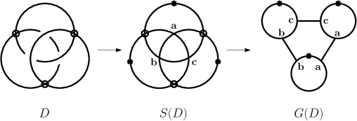
As stated above, the number of alternately coloured smoothings is a link invariant, so that we are free to use the Gauss diagram associated to any diagram of .
As observed by Kauffman [8] alternately coloured smoothings of a link diagram are in bijection with particular colourings of the shadow of the diagram: colouring the arcs of the shadow either red or green such that at every classical crossing we have the following (up to rotation):
Such a colouring is known as a proper colouring. Given a virtual link diagram and a proper colouring of , one produces an alternately coloured smoothing of by resolving each classical crossing in the manner dictated by the proper colouring i.e. joining red to red and green to green. Two examples are given in Figure 11. It is easy to see that this association defines a bijection between the set of proper colourings and the set of alternately coloured smoothings.
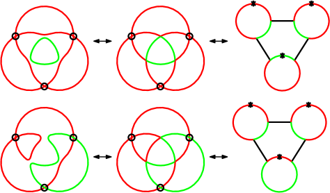
Next, notice that a proper colouring of induces a colouring of the circles of : colour the connected components of the complement of the chord endpoints in the manner dictated by the colouring of the shadow (so that when an endpoint is passed the colour changes). A Gauss diagram coloured in such a way is known as alternately coloured. Examples are given in Figure 11. It is again easy to see that alternately coloured Gauss diagrams are in bijection with proper colourings, so that we have a bijection between alternately coloured smoothings of and alternate colourings of .
In light of the above we see that we are required to verify that a Gauss diagram of circles has alternate colourings if and only it has no degenerate circles.
Let contain a degenerate circle. On this circle the number of connected components of the complement of the end points is odd, from which we deduce that it cannot be alternately coloured (as the colour must change when passing an endpoint). That there are alternate colourings if there is no degenerate circle follows from the observation that there are two possible configurations for each circle, and that given an alternate colouring flipping the configuration on one circle yields a new alternate colouring. ∎
Corollary 3.13.
Let be a virtual knot. Then and is supported in homological degree equal to the height of the alternately colourable smoothing.
Proof.
Let be a virtual knot diagram. Then satisfies the condition of Theorem 3.12 as it contains only one circle, on which all chord endpoints must lie. Of course, every chord has two endpoints so that this circle must contain an even number of them. The statement then follows from Theorem 3.5. ∎
Classically, the alternately colourable smoothing of an oriented knot diagram is its oriented smoothing. Classical Khovanov homology is rigged so that this smoothing is at height , and subsequently classical Lee homology of a knot is supported in homological degree . This is no longer the case with doubled Lee homology: virtual knot (given in Figure 6) provides an example of a knot for which the alternately colourable smoothing is, in fact, the unoriented smoothing. Taking the connect sum of with any classical knot yields a virtual knot for which the alternately colourable smoothing is neither the oriented nor the unoriented smoothing. The height of the alternately colourable smoothing of a knot shall be used in the definition of the doubled Rasmussen invariant in Section 4, and is shown to be equal to the odd writhe of the knot in Section 4.3.
Corollary 3.14.
Let be a split link of components. Then .
3.2. Interaction with cobordisms
A cobordism between classical links defines a map on classical Lee homology; this behaviour is replicated by doubled Lee homology. Unlike the classical case, however, many connected cobordisms must be assigned the zero map, a consequence, for example, of the vanishing of for certain links or of the possibility of doubled Lee homology of knots being supported in non-zero homological degrees. Nevertheless, there are classes of cobordisms for which the associated maps are non-zero (some of which we use in Section 5). In this section we verify that concordances and a certain class of arbitrary genus cobordisms are assigned non-zero maps.
We begin by stating some definitions regarding virtual cobordism (see [9]).
Definition 3.15.
Two virtual links and are cobordant if a diagram of one can be obtained from a diagram of the other by a finite sequence of births and deaths of circles, oriented saddles, and virtual Reidemeister moves. Such a sequence describes a compact, oriented surface, , such that . Births of circles, oriented saddles, and deaths of circles correspond, respectively, to -, -, and -handles of . If we say that and are concordant. If is a knot concordant to the unknot we say that is slice. In general, we define the slice genus of a virtual knot , denoted , as
(here we have simply capped off the unknot in with a disc).
Virtual links are equivalence classes of embeddings of disjoint unions of into thickened surfaces [13]; thus the surface is embedded in a -manifold of the form where is a compact, oriented -manifold with , where denotes a closed surface of genus . The -manifold is described in the standard way in terms of codimension submanifolds and critical points: starting from , codimension submanifolds are until we pass a critical point, after which they are . Critical points of correspond to handle stabilisation (induced by virtual Reidemeister moves). A finite number of handle stabilisations are made to reach . We say that a link appears in if a diagram of it appears in the sequence of diagrams describing .
Of course, the subject of Definition 3.15 is really a presentation of a cobordism; two distinct presentations may be equivalent under isotopy (relative to their boundary), and represent the same cobordism. However, as mentioned by Rasmussen and others in the classical case, we expect isotopic presentations to be assigned the same map. Like Rasmussen, we do not pursue this further, and suffice ourselves with working with presentations. Moreover, we shall ignore the difference between a presentation and a cobordism, referring to the surface as a cobordism between and .
Definition 3.16.
Let be a cobordism between two virtual links and which is described by exactly one virtual Reidemeister move or one oriented -,-, or -handle addition. Such a cobordism is known as elementary.
We wish to associate maps to cobordisms such that, where they are non-zero, the maps respect the filtration and send alternately coloured generators (of the homology of the intitial link) to linear combinations of alternately coloured generators (of the homology of the final link).
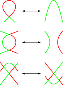
Of course, any cobordism can be built by gluing elementary cobordisms end to end, so we shall first investigate these simple cobordisms. In all there are ten of them: four given by the purely virtual Reidemeister moves and the mixed move, three given by the classical Reidemeister moves, and three given by the -, , and -handle additions. We separate the work into elementary cobordisms which contain virtual Reidemeister moves and those which contain handle additions.
(Virtual Reidemeister moves): Let and be diagrams of virtual links and , and an elementary cobordism between them which contains a purely virtual Reidemeister move or mixed move (as depicted in Figure 4). Then , as such moves preserve the number of cycles in a smoothing and the incoming and outgoing differentials. Thus we associate to the map . It is also clear that such a cobordism sends alternately coloured smoothings of to those of , so that alternately coloured generators of are sent to those of .
If contains a classical Reidemeister move then is one of the maps defined in [19, Section ], with the addition of the appropriate superscripts. We satisfy ourselves with a quick demonstration that classical Reidemeister moves send alternately coloured smoothings to alternately coloured smoothings, via proper colourings of shadows. As mentioned above, given a virtual link diagram , the set of its alternately coloured smoothings is in bijection with the set of proper colourings of its shadow. Let and be related by a classical Reidemeister move. Then and are identical except within a neighbourhood of the move. Given a proper colouring of define a proper colouring of which is identical to that of outside the proscribed neighbourhood; the colouring within is dictated by that of arcs incident to the neighbourhood. Some examples are given in Figure 12. It is clear that this defines a bijection between the proper colourings of and those of , and it follows that the maps associated to the classical Reidemeister moves are isomorphisms on doubled Lee homology.
(Handle additions): Let and be diagrams of virtual links and , and an elementary cobordism between them which contains a handle addition. Then defines a map of cubes between the cube of smoothings of and that of : removing a neighbourhood of the classical crossings of and , both diagrams look identical except in the region in which the handle is attached. Moreover, as handle additions do not change the number of crossings of diagram, the smoothings of and are in bijection (a string of ’s and ’s defines uniquely a smoothing of and of ). Let the map of cubes defined by be the map which sends a smoothing of to the associated smoothing of . As the diagrams are identical exept in a small region this map acts simply on smoothings, and depends on the handle addition contained in :
-
•
-handle: a cycle is added which shares no crossings with any other cycle or itself.
-
•
-handle: two cycles are merged into one cycle, one cycle is split into two, or one cycle is sent to one cycle (while the -handle is necessarily oriented, it is nonetheless possible for it to induce such a term as a map of cubes.)
-
•
-handle: a cycle which shares no crossings with any other cycle or itself is removed.
Thus we define a map , whose affect on the specific cycle or cycles involved is as follows (and acts as the identity on the uninvolved cycles)
-
•
-handle: where , so that , for example.
-
•
-handle: either , , or as dictated by the corresponding entry in map of cubes.
-
•
-handle: where , .
We define to be the map induced by . Notice that is filtered of degree for - and -handle additions and filtered of degree for -handle additions, and that it preserves homological degree.
Definition 3.17.
Let and be diagrams of virtual links and , and a cobordism between them. Then can be decomposed as a finite union of elementary cobordisms, so that
where is an elementary cobordism. Define .
It is possible that a map associated to a cobordism is necessarily zero, owing to the doubled Lee homology of a link (or links) appearing in it being trivial in particular degrees (or possibly every degree). Homological degrees which survive throughout a cobordism are important, therefore.
Definition 3.18.
Let and be diagrams of virtual links and , and a cobordism between them such that the doubled Lee homology of every link appearing in it is non-trivial in homological degree . Such a homological degree is known as a shared degree (of ).
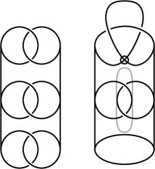
The existence of shared homological degrees is not enough to guarantee that a cobordism is assigned a non-zero map, however. Consider the cobordism depicted in Figure 13: the left-hand component is the identity cobordism on the classical Hopf link, while the right-hand component is a genus cobordism from virtual knot to the unknot. It can be quickly verified that is a shared degree of this cobordism, but that the map assigned to it is zero.
The remainder of this section is concerned with the task of verifying that concordances and some arbitrary genus cobordisms are assigned non-zero maps, as advertised above. In what follows, a cobordism is said to be weakly connected if every connected component has a boundary component in the initial link.
Theorem 3.19.
Let be a concordance between a virtual knot and a virtual link . Suppose that contains no closed components and that . Then is non-zero.
Theorem 3.20.
Let be a weakly connected cobordism between virtual knots and with a non-empty set of shared degrees. Further assume that can be decomposed as the union of two cobordisms, and , such that where is a virtual link. Suppose that, in addition to virtual Reidemeister moves, contains only -handles between a single link component, and handles between distinct link components. There is exactly one alternately colourable smoothing of , denoted , such that the associated generators are in the image of , and a finite set of alternately colourable smoothings of , denoted , such that the associated generators are in the cokernel of . Then is non-zero if and only if .
A cobordism satisfying the criteria of Theorem 3.20 is known as a targeted cobordism.
We begin our path to the proofs of Theorems 3.19 and 3.20 by investigating elementary cobordisms; many maps assigned to them are non-zero automatically.
Proposition 3.21.
Let and be diagrams of virtual links and , and an elementary cobordism between them which is a - or -handle addition, or a -handle addition between two distinct link components. If has a non-zero number of alternately coloured smoothings, then has shared degrees and is non-zero in them.
Proof.
We are required to verify two criteria : that has at least one alternately coloured smoothing at the same height as one of the alternately coloured smoothings of , and : that sends at least one alternately coloured generator of to a linear combination of those of . For - and -handles follows from the fact that the cycle being added or removed does not take part in any of the crossings in or , and thus places no restrictions on a smoothing being alternately coloured. As an handle addition does not change the number of classical crossings it is clear that an alternately coloured smoothing of is sent to an alternately coloured smoothing of of the same height. Further, noticing that
| (3.7) | ||||
we see that is satisfied. (Note that -handles double the number of alternately coloured smoothings, while -handles halve it.)
For -handle additions between two distinct link components we verify in the following manner: consider the Gauss diagrams and . By assumption contains no degenerate circles. As the -handle consituting is between two distinct link components, can be obtained from by combining two circles (those corresponding to the components between which the handle is added) and adding all chord endpoints which lie on them to the new circle, leaving the other circles unchanged. Thus the number of chord endpoints lying on the new circle must be a multiple of and it is not degenerate. As the other circles are unchanged it is clear that has no degenerate circles and has alternately coloured smoothings - note that it has half the number that has, however. That there are heights at which both and have alternately coloured smoothings again follows from the fact that handle additions do not change the number of classical crossings. The statement follows from Equations 3.5 and 3.6. ∎
In the case of -handles involving a single link component we are able to determine whether they preserve the existence of alternately coloured smoothings by looking at their effect on Gauss diagrams. Using this we can specify the handle additions which are associated non-zero maps.
Lemma 3.22.
Let and be diagrams of virtual links and , and an elementary cobordism between them which is a -handle addition involving a single link component. Further, assume is non-trivial. Then is trivial if and only if there is a proper colouring of such that the handle addition is between two strands of opposite colour.
Proof.
It follows from Theorem 3.5 that is trivial if and only if has no alternately coloured smoothings. Consider the Gauss diagram of the shadow of : as the handle addition is between a single link component it can be represented in the following manner:
![[Uncaptioned image]](/html/1704.07324/assets/x40.png)
On the left the circle of corresponding to the component of undergoing the handle addition is depicted; the dotted line shows the location of the handle addition. Clearly, if the handle is added between two regions of opposite colour the dotted line must enclose an odd number of chord endpoints, so that the newly created circles are degenerate (as depicted on the right). Conversely, it is easy to see that if the handle is between two regions of the same colour then the newly created circles are non-degenerate. To conclude, note the regions are either both coloured the same colour in all proper colourings of or are coloured opposite colours in all proper colourings, as all proper colourings are related by flipping the colours on a finite number of circles. ∎
Corollary 3.23.
Let and be diagrams of virtual links and , and an elementary cobordism between them which contains a -handle addition between a single link component. Further, assume that is non-trivial and that the -handle addition is between strands of the same colour in . Then has shared degrees and is non-zero in them.
We omit the proof of Corollary 3.23 as it uses very similar ideas to that of Proposition 3.21 along with Equations 3.5 and 3.6.
Using the map of cubes defined by a handle addition (see figure 12) we continue to investigate the maps associated to -handle additions further. In what follows we shall suppress the upper/lower subscripts of the generators , as it easy to see that if and only if . Also, whenever we state equalities such as , for example, we shall always mean equality up to a (non-zero) scalar.
Proposition 3.24.
Let and be diagrams of virtual links and , and an elementary cobordism between them which is a -handle addition. Further let and be non-trivial. (Recall that the smoothings of and are in bijection.) There are two cases:
-
(i)
if the -handle is between two distinct components of , then every alternately coloured smoothing of is associated to an alternately coloured smoothing of .
-
(ii)
if the -handle involves a single component of , then every alternately coloured smoothing of is associated to an alternately coloured smoothing of .
(A smoothing of is associated to a smoothing of if and only if it is sent to it under the map of cubes defined by .)
Proof.
As observed in Section 3 the alternately coloured smoothings of a diagram are in bijection with the proper colourings of the shadow of the diagram. In case one readily observes that a proper colouring of defines a proper colouring of (as the handle must join two strands of the same colour, a consequence of Lemma 3.22). Moreover this proper colouring of induces the same crossing resolutions as those of the proper colouring of , so that corresponding alternately coloured smoothings are associated. In case , notice that the reverse cobordism (from to ) satisfies . ∎
Corollary 3.25.
Let and be diagrams of virtual links and , and an elementary cobordism between them which is a -handle addition with shared degrees. Then, for a shared degree
-
(i)
If the handle addition is between two distinct components of then surjects onto .
-
(ii)
If the handle addition is between a single component of then for all .
Proof.
: Let be defined by an alternately coloured smoothing of . Then by Proposition 3.24 is associated to , an alternately coloured smoothing of (and is mapped to it under the map of cubes defined by ). Let denote the alternately coloured generator of defined by . If acts by either or on then automatically (by Equations 3.5 and 3.6). If it acts by , then it is possible that , if the cycles undergoing the merge map are coloured opposite colours. Notice that if is obtained from by merging two cycles, then is obtained from by splitting two cycles. As observed in the proof of Proposition 3.24, by looking at proper colourings and associated to and , respectively, we see that the relevant cycles cannot be coloured opposite colours in ; thus (again by Equation 3.5).
: Let be defined by the alternately coloured smoothing of . By Lemma 3.22 the handle addition must be between cycles of the same colour in so that by Equations 3.5 and 3.6. ∎
Proof of Theorem 3.19.
First we shall prove a fact about links appearing in concordances, before using this fact and an induction argument to prove the theorem in this restricted case.

Let be a concordance between a virtual knot and a virtual link such that . Assume towards a contradiction that a link, , appearing in is such that . By Theorems 3.5 and 3.12, must contain a degenerate circle, for any diagram of . Further, by Lemma 3.22, we see that degenerate circles are always created in pairs in a cobordism, and that degenerate circles can be cancelled against one another to produce non-degenerate circles (see Figure 14). This cancelling process is as follows: add a -handle between the components of which correspond to the degenerate circles, producing a new circle. Let the two initial degenerate circles be and , and denote the number of chord endpoints lying on . It is easy to see that the number of chord endpoints lying on the newly created circle is , and that must be even as and are odd. Thus the newly created circle is non-degenerate.
In what follows we shall call a component of a link diagram degenerate if the circle corresponding to it in the associated Gauss diagram is degenerate. We may also speak of degenerate components of links, as virtual Reidemeister moves cannot change the mod number of chord endpoints lying on a circle.
As has non-trivial doubled Lee homology (it is a knot), no diagram of it contains a degenerate component. Therefore at least one -handle involving a single link component must occur in to produce (recall again Lemma 3.22). As also has non-trivial doubled Lee homology, we see that we must remove all degenerate link components (by the process outlined above) in order to reach from . But degenerate circles are always formed in pairs, and we see that an attempt to cancel them all without introducing genus - which we are prohibited from doing as is a concordance - leads to a non-compact situation; consider Figure 14. As we are considering only compact cobordisms (recall Definition 3.15) we arrive at the desired contradiction.
We now present the aforementioned induction argument: we shall build up concordances with elementary cobordisms. Let be a concordance between a virtual knot and virtual link (distinct from , , and above) such that contains no closed components, and is non-zero. We claim that if is an elementary cobordism between and such that then is non-zero also. Note that the argument above implies that we may restrict to the case in which : if this did not hold then could not form part of a concordance between links which both have non-trivial doubled Lee homology.
If is a virtual Reidemeister move or a -handle addition then is non-zero as has trivial kernel. If is a -handle addition then is spanned by the image of the map associated to a -handle addition. But if a -handle addition preceeds then would contain a closed component, which it does not by assumption, so that is non-zero.
If is a -handle involving a single link component we see that has trivial kernel by Corollary 3.25, as we are working in the case in which .
We are left with the case in which is a -handle between distinct link components. If is to have genus the link components of involved in must be belong to different connected components of . As begins with , a virtual knot, at least one of the components of involved in must be have no boundary component in i.e. its first appearance in is a -handle. (Cutting the cobordism depicted in Figure 14 at the link labelled yields an example.)
Let . We can write , where is an alternately coloured generator of . Let denote the alternately coloured smoothing of which defines , and the associated proper colouring of the shadow (of the appropriate diagram) of . Then if and only if the link components of involved in are coloured opposite colours in every (recall the bijection between components of a link diagram and components of its shadow given in Definition 3.9). This can be seen from Equation 3.5.
As observed above, at least one of the connected components of involved in begins with a -handle, and Equation 3.7 shows that the image of the map assigned to a -handle is a linear combination of both red and green. Therefore, given an arc of lying on a component which begins with a -handle, if has the arc labelled a particular colour, there must exist a in which the arc is coloured the opposite colour, and is non-zero.
The base cases of the induction are the elementary cobordisms: they are all clearly of genus and satisfy the induction hypothesis, under our assumption that both the initial and terminal links have non-trivial doubled Lee homology. Thus, given a concordance between a virtual knot and a virtual link with non-trivial doubled Lee homology, the assigned map is non-zero. ∎
Proof of Theorem 3.20.
Let , , and be as in the theorem statement. The cobordism is a concordance between a link and a knot, and so is non-zero by Theorem 3.19. Recall that is the set of alternately colourable smoothings of such that the associated generators are in the cokernel of ; this is necessarily non-empty as is non-zero. Further, has trivial kernel (as observed in the proof of Theorem 3.19) so that is of rank , spanned by the alternately coloured generators associated to exactly one smoothing of , namely : to see this, recall that , so that if the generators associated to more than one smoothing of lay in the image of , it could not be of rank (generators associated to different smoothings are linearly independent). By assumption so that, if are the generators associated to , then and is non-zero. ∎
Remark.
In proving Theorems 3.19 and 3.20 we could not follow Rasmussen’s approach of propagating orientations through the cobordism, as we no longer necessarily have the relationship between orientations of a link and its alternately coloured smoothings. Also, while all the maps associated to elementary cobordisms are non-zero (as long as the homologies do not vanish), the full map associated to may fail to be non-zero without requiring a non-empty set of shared degrees (in the classical case every cobordism has shared degree ). Moreover, the proof in the classical case is concerned only with this degree, while we must investigate the map associated to cobordisms in every homological degree.
4. A doubled Rasmussen invariant
As demonstrated in the preceding section, for an oriented virtual knot, , is a rank bigraded group, supported in a single homological degree which can be determined easily from any diagram of . In Section 4.1 we show that the data provided by the quantum gradings in which is supported are equivalent to a single integer (in the classical case this integer is necessarily even), so that the information contained in is equivalent to a pair of integers. In Section 4.2 we give some properties of this pair of integers. and in Section 4.3 we show that one of the members of the pair is equal to the odd writhe of the given knot. Finally, in Section 4.4 we describe a class of knots for which the invariant can be quickly calculated.
4.1. Definition
We referred to a filtration of in Definition 3.1 - let us concretise it (following Rasmussen [19]). Let be an oriented virtual knot diagram of with positive classical crossings and classical crossings. The homological grading on , denoted , is as defined in Equation 2.4. The quantum grading is the standard one: define , , , , , then the quantum grading is the shift . Let , so that we have the filtration
for some ; let denote the associated grading i.e. if and .
Definition 4.1.
For a virtual knot let
| (4.1) | ||||
and similarly define .
That can be determined from (and vice versa) follows in large part from the following augmented version of [19, Lemma ].
Lemma 4.2.
For a virtual knot
where is generated by elements of quantum grading congruent to . Further
-
(i)
Either
or
-
(ii)
Either
or
Here denotes an alternately coloured generator as defined in Equation 3.4, and denotes the generator formed by replacing with and with .
Proof.
That decomposes into the given direct sum follows from the form of the differential: a part graded of degree and other graded of degree . The statements within are obvious consequences of the construction of .
We are left with : the mod behaviour of the quantum grading is complicated by the fact that doubled Khovanov homology is supported in both odd and even quantum gradings, a departure from the classical case. We shall prove the case when ; this corresponds to the first statement in , the second follows identically modulo a grading shift.
Following Rasmussen, define so that acts by the identity on and by multiplication by on . Next, define by and . Then and , and acts as the identity on and by multiplication by on . Thus we have
which yields
from which we deduce that and . We conclude by invoking . ∎
Corollary 4.3.
Let be a virtual knot. Then
Proposition 4.4.
Let be a virtual knot. Then
Proof.
Consider the map
induced by the connect sum (this is well-defined as it is between and a crossingless unknot diagram). This is well-defined, preserves homological degree, and with respect to the quantum degree is graded of degree (as it is simply ). Again we follow Rasmussen and denote the alternately coloured generators of by their decoration at the connect sum site i.e. and . The alternately coloured generators of are then , , , and . Under we have
Noticing that and
we obtain
as is graded of degree (that follows from Lemma 4.2). ∎
Thus any of the four quantities defined in Definition 4.1 determines all of the others and we able to make the following definition.
Definition 4.5.
For a virtual knot let where
where denotes homological grading and an alternately coloured generator of associated to the alternately coloured smoothing . We refer to as the doubled Rasmussen invariant of .
4.2. Properties
Proposition 4.6.
For a classical knot , where denotes the classical Rasmussen invariant.
Proof.
For a classical knot decomposes as
so that clearly , where denotes the classical quantity. Then
That is observed on corollary 3.13. ∎
The doubled Rasmussen invariant exhibits the same behaviour with respect to mirror image and connect sum as its classical counterpart.
Proposition 4.7.
Let be a virtual knot denote its mirror image. Then .
Proof.
The statement follows, as in the classical case, from the existence of the isomorphism of dual complexes
That is seen as follows: let be a diagram of with positive classical crossings and negative classical crossings. Let be the alternately colourable smoothing of , so that , the height of . Further, notice that
where
and likewise and (for a classical knot , of course). It is quickly observed that
where denote the corresponding quantities for . Then
∎
Proposition 4.8.
Let and be virtual knots and denote by any of their connect sums. Then
Proof.
It is readily apparent that , where / / is the alternately colourable smoothing of / / . Then , which proves the claim regarding .
Let be the map realised by acting on the cycle as dictated by the connect sum. Regarding , the proof follows in identical fashion to the classical proof when one notices that we only require the existence of (as opposed to the short exact sequence used in [19]). ∎
4.3. Relationship with the odd writhe
Kauffman defined the odd writhe of a virtual knot in terms of Gauss diagrams [8]. In this section we show that the doubled Rasmussen invariant contains the odd writhe.
Definition 4.9.
Let be a diagram of a virtual knot and its Gauss diagram. A classical crossing of , associated to the chord labelled in , is known as odd if the number of chord endpoints appearing between the two endpoints of is odd. Otherwise it is known as even. The odd writhe of is defined
Theorem 4.10.
Let be a virtual knot diagram of . The odd writhe is an invariant of and we define
The odd writhe of a virtual knot provides a quick way to calculate .
Proposition 4.11.
Let be a diagram of a virtual knot . Then .
Proof.
We claim that a classical crossing in is odd if and only if it is in its unoriented resolution in the alternately colourable smoothing of .
(): Let denote an odd classical crossing of . Leaving the crossing from either of the outgoing arcs we must return to a specified incoming arc. Between leaving and returning we have passed through an odd number of classical crossings (which are not ). Thus the incoming arc must be coloured the opposite colour to the outgoing, and is resolved into its unoriented resolution in the both of the alternately coloured smoothings of , as depicted here:
![[Uncaptioned image]](/html/1704.07324/assets/x45.png)
(): Let denote a classical crossing of which is resolved into its unoriented smoothing in the alternately colourable smoothing of . The colouring at must be as depicted above. Again, leaving from either outgoing arc and returning at the specified incoming arc, we see that, as the colours of the arcs are opposite, an odd number of classical crossings must have been passed.
The contributions of odd and even crossings to and are summarised in the following table, from which the result follows. The contributions to are clear when one recalls that the height of a smoothing contains the shift , the total number of negative classical crossings of .
| sign | parity | reso. | ||
|---|---|---|---|---|
| odd | ||||
| even | ||||
| odd | ||||
| even |
∎
Corollary 4.12.
Let and be virtual knots and denote any of their connect sums. Then
4.4. Leftmost knots and quick calculations
To conclude this section we identity a class of knots for which the calculation of the doubled Rasmussen invariant is trivial, a generalisation of the case of computation of the classical Rasmussen invariant of positive classical knots. The key here, as in the classical case, is that the alternately coloured smoothings of the class of knots in question have no incoming differentials.
Definition 4.13.
Let be a virtual knot diagram. We say that is leftmost if it contains only positive even and negative odd classical crossings. A virtual knot is leftmost if it has a leftmost diagram.
Proposition 4.14.
Let be a leftmost diagram of a virtual knot with negative classical crossings. Then , the minimal non-trivial homological grading of .
Proof.
Let be a leftmost diagram of a virtual knot. By Proposition 4.11 we have , as a crossing in is odd if and only if it is negative. ∎
Proposition 4.15.
Let be a leftmost diagram of a virtual knot . Then , where is an alternately coloured generator associated to the alternately colourable smoothing of .
Proof.
By Proposition 4.14 the alternately colourable smoothing of is at the minimal non-trivial height of the cube of resolutions. By construction there is only one smoothing at this height. Further, this smoothing has no incoming differentials. Recalling Definition 4.5, we obtain the result. ∎
5. Applications
We shall now describe some applications of the invariants and . All of the given applications are related to virtual link concordance, to a greater or lesser extent.
5.1. Cobordism obstructions
As mentioned in Section 3.2, we can use the information contained in the quantum degree of to obtain obstructions to the existence of cobordisms between and other links. First we repeat the procedure used to show that the classical Rasmussen invariant yields a bound on the slice genus to obtain a bound on the genus of a certain class of cobordisms from a knot to the unknot, and between two given knots. We then obtain an obstruction to the existence of a concordance between a link and a given knot. Finally, we use doubled Lee homology to show that virtual knots with non-zero odd writhe are not slice.
5.1.1. Genus bounds
In this section we use the fact that concordances and targeted cobordisms are assigned non-zero maps to obtain obstructions to the existence of cobordisms of certain genera between pairs of virtual knots. First we obtain a lower bound on the genus of targeted cobordisms between pairs of knots whose invariants agree.
Theorem 5.1.
Let be a virtual knot with and a targeted cobordism from to the unknot such that is a shared degree of . Then
| (5.1) |
Proof.
Let and be as in the theorem statement. Then, by Theorem 3.20, is a non-zero map. As in the classical case, it is easy to see that is filtered of degree . Let realise so that
as . This yields
Repeating the argument for , and using Proposition 4.7, we obtain
which yields the desired result. ∎
Corollary 5.2.
Let be a virtual knot with and a targeted cobordism from to the unknot such that . Then there exists a link which appears in with .
In a very similar manner we able to show the following.
Theorem 5.3.
Let and be a pair of virtual knots with , and be a targeted cobordism between them such that is a shared homological degree of . Then
Further, concordances between virtual knots are obstructed by the quantum degree component of the doubled Rasmussen invariant, (in Section 5.1.3 we show that the homological component is such an obstruction, also).
Theorem 5.4.
Let and be virtual knots such that . If then and are not concordant.
The proof of Theorem 5.4 follows almost exactly along the lines of that of Theorem 5.1, which itself is very similar to the classical case; all we require is that the map assigned to a concordance is non-zero, which is verified in Theorem 3.19.
Corollary 5.5.
Let be a virtual knot with . If then is not slice.
5.1.2. Obstructions to concordances between knots and links
We can extend Theorem 5.4 to the case in which one end of the concordance is a link, provided the homologies of the knot and link in question are compatible, and the concordance is connected.
Theorem 5.6.
Let be a virtual link of components. Further, let be a connected concordance between and a virtual knot such that . Let be the maximum non-trivial quantum degree of elements such that . Then
Proof.
Let , , and be as in the theorem statement. Then is non-zero by Theorem 3.19. It is clear that is filtered of degree : a minimum of -handles are needed to take a -component link to a knot, and any surplus -handles must be paired with -handles. It is also clear that if is such that then . For such an we have that and
so that
as required. ∎
Corollary 5.7.
Let be a virtual link of components such that . Further, let a virtual knot such that is trivial in homological degree or
Then any concordance from to is disconnected.
A particular consequence of Corollary 5.7 is that, given a virtual link for which and , all concordances from to classical knots must be disconnected: no classical knots can be obtained from by simply merging its components.
5.1.3. The odd writhe is an obstruction to sliceness
The odd writhe of a knot is very easy to calculate. Despite this it can detect non-classicality (and hence non-triviality) and chirality of many virtual knots [8]. Here we show that it also contains information regarding the concordance class of a virtual knot.
Theorem 5.8.
Let be a virtual knot. If then is not slice.
Proof.
We prove the contrapositive. Assume towards a contradiction that is a slice virtual knot such that . Then by Proposition 4.11. Let realise a slice disc so that is non-zero by Theorem 3.19. Recall that preserves homological degree by construction. There must exist such that . But then
as , a contradiction. ∎
The proof of Theorem 5.8 can be used mutatis mutandis to show that the set of concordance classes of virtual knots is partitioned by the odd writhe.
Theorem 5.9.
Let and be virtual knots. If then and are not concordant.
Corollary 5.10.
Let be a virtual knot. If then is not concordant to a classical knot.
5.1.4. Examples
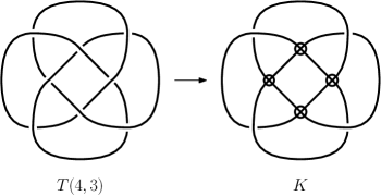
Consider the classical knot , as given in Figure 15. By converting a particular subset of its crossings to virtual crossings we are able to produce a virtual knot, , whose alternately colourable smoothing is its oriented smoothing ( is also positive, as is). Thus and the odd writhe provides no obstruction to sliceness. However, is a leftmost knot (as defined in Section 4.4), so that by Proposition 4.15. It can be quickly verified that so that is not slice by Corollary 5.5.
Further, consider the classical two-component link , as depicted in Figure 16. By an argument identical to that used in the case of leftmost knots we can show that the maxiumum quantum degree of all elements in is . In the context of Theorem 5.6, considering connected concordances from to the unknot, and as , it follows that there does not exist a connected concordance from to the unknot.
The method used in both the above examples can be applied to many positive oriented classical link diagrams in order to produce virtual link diagrams for which the quantum degree information (at particular homological degrees) is easy to compute.
5.2. Connect sums of trivial diagrams
First let us recall the definition of the connect sum of virtual knot diagrams (see [16]).
Definition 5.11.
Let and be oriented virtual knot diagrams. If is such that there exists a disc with and (where denotes an oriented unit interval and an interval with reverse orientation) then we denote by the diagram produced by -handle addition with attaching sphere .
The connect sum operation is well defined on classical knots. As mentioned in Section 1.1, this is not the case for virtual knots. Given a pair of virtual knots and with diagrams and , respectively, the result of the connect sum operation depends on the diagrams used and the choice of disc . By an abuse of notation we use to refer to any of the knots produced by a connect sum operation on and .
There are two ways in which to interpret the ill-defined nature of the connect sum operation on virtual knots. The first is in a diagrammatic manner: no longer can one area of the diagram be freely moved over all others, due to presence of the forbidden moves. These are moves on diagrams, depicted in Figure 17, which do not follow from the virtual Reiedemeister moves (in fact, they can be used to unknot any virtual knot [18]). Classically, Reidemeister moves commute, in a certain sense, with handle addition: for example, let and be classical unknot diagrams. Then can be treated as a small neighbourhood of and slid under (or over) the rest of the diagram. Thus the sequence of Reidemeister moves which takes to the crossingless unknot diagram can be replicated on , taking it to , which is itself an unknot diagram. Nontrivial diagrams are treated similarly. Virtually, however, this cannot be replicated as areas of a diagram cannot always be moved across others.
The second, deeper, interpretation is as a consequence of the higher-dimensional topological information constituting a virtual knot: as mentioned above, a virtual knot is an equivalence class of embeddings of into thickened closed orientable genus surfaces, up to isotopy of the thickened surface and handle stabilisations of the (unthickened) surface [7]. Not only does a virtual knot depend on how the copy of is knotted about itself but also on how it is ‘knotted’ about the topology of the thickened genus surface into which it is embedded.
In this light we see that the connect sum operation is not only a -dimensional -handle addition between the copies of , but that it also induces a -dimensional -handle addition on the thickened genus surfaces111it is possible for the connect sum operation not to induce a -dimensional handle addition but a slightly more complicated operation. We refer the reader to [17, page 41, Fig. ].. This contrasts with the classical case in which both copies of can be contained in one copy of and only a -dimensional -handle need be added. Different choices of the disc (as in Definition 5.11) correspond to different choices of -dimensional handles. The author suspects that the dependence of the connect sum operation on both the diagrams involved and the choice of is inherited ultimately from the non-triviality of the fundamental group of a genus surface.
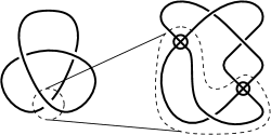
A novel manifestation of this ill-definedness is that there exist non-trivial virtual knots which are connect sums of a pair of trivial virtual knots. The first example of this is given by Kishino’s knot [12] as depicted in Figure 18. Doubled Khovanov homology yields a condition on a virtual knot being a connect sum of two trivial diagrams.
Theorem 5.12.
Let be a virtual knot which is a connect sum of two trivial knots. Then .
In order prove to Theorem 5.12 we shall define a reduction of doubled Khovanov homology, in direct analogy to the classical case [11, 20].
Definition 5.13 (Reduced doubled Khovanov homology).
Let be an oriented virtual link diagram with a marked point on each component (away from the crossings of ). Distribute these marked points across the cube of smoothings so that each smoothing of contains marked points. Define to be the chain subcomplex of spanned by those states in which all the marked cycles are decorated with either or (all the marked cycles are decorated with the same algebra element). That is a subcomplex is evident from Equations 2.3 and 2.2 (it is also graded).
Let denote the homology of . We refer to as the reduced doubled Khovanov homology of .
The proof of invariance of under virtual Reidemeister moves follows as in the classical case. Invariance under the choice of basepoints follows similarly.
Lemma 5.14.
Let be a virtual link diagram. Then .
Proof.
We prove the statement for a virtual knot diagram (link diagrams follow essentially identically). Let . The isomorphism is straightforward to define. Given a representative, , of an element of the marked cycle must be decorated with either or i.e. we must have . Define
That is well defined is clear and that it is a chain map is apparent when one considers the schematic given in Figure 19: the only issue that could arise is due to the factor of in the map, the position of which ensures that it does not cause any trouble. That the degree of is is obvious.

∎
Proof of Theorem 5.12 .
Let be as in the proposition. By an abuse of notation let be the diagram which is the result of a connect sum between and , both of which are unknot diagrams. We are free to pick marked points on the diagrams and so that the situation is as in Figure 20, from which we observe that there is a chain complex isomorphism from . The isomorphism is defined as follows
where and decorate the marked cycles. That is a chain map follows from the observation that if is a state of then has the same incoming and outgoing differentials. It is clear that is graded of degree .
We have established the isomorphism ; further, there is a chain homotopy equivalence between and as and are unknot diagrams. It is easy to see that so that
and
| (5.2) |
In addition, there is an exact triangle
| (5.3) |
which is arrived at via the short exact sequence
Lemma 5.14 and the observation that Equation 5.2 implies that is supported in homological degree . Also by Equation 5.2 we obtain so that the triangle splits and

∎
Proposition 5.15.
Let and be virtual knots which are connect sums of the same pair of initial virtual knots and : that is, there exist diagrams and of and and of such that and . Then .
Proof.
We have , as and are both diagrams of and the isomorphisms are essentially identical to that given in the proof of Theorem 5.12. ∎
Remark.
Of course, there is still a pair of short exact sequences
but the associated long exact sequences no longer split. Indeed, it is not true in general that
the aforementioned virtual knot provides a counterexample.
References
- [1] D Bar-Natan. On Khovanov’s categorification of the Jones polynomial. Algebraic & Geometric Topology, 2, 2002.
- [2] D Bar-Natan and H Burgos-Soto. Khovanov homology for alternating tangles. Journal of Knot Theory and its Ramifications, 23, 2014.
- [3] D Bar-Natan and S Morrison. The Karoubi envelope and Lee’s degeneration of Khovanov homology. Algebraic & Geometric Topology, 6, 2006.
- [4] H A Dye. Virtual knots undetected by 1- and 2-strand bracket polynomials. Topology and its Applications, 153, 2005.
- [5] H A Dye, A Kaestner, and L H Kauffman. Khovanov Homology, Lee Homology and a Rasmussen Invariant for Virtual Knots. Journal of Knot Theory and Its Ramifications, 26, 2017.
- [6] J Green. A Table of Virtual Knots. https://www.math.toronto.edu/drorbn/Students/GreenJ/index.html.
- [7] L H Kauffman. Virtual Knot Theory. European Journal of Combinatorics, 20, 1999.
- [8] L H Kauffman. A self-linking invariant of virtual knots. Fundamenta Mathematicae, 184, 2004.
- [9] L H Kauffman. Virtual knot cobordism. New Ideas in Low Dimensional Topology, 2015.
- [10] L H Kauffman and D Radford. Bi-oriented quantum algebras, and a generalized alexander polynomial for virtual links. Contemporary Mathematics, 318, 2003.
- [11] M Khovanov. A categorification of the Jones polynomial. Duke Mathematical Journal, 101, 1999.
- [12] T Kishino and S Satoh. A note on non-classical virtual knots. Journal of Knot Theory and Its Ramifications, 13, 2004.
- [13] G Kuperberg. What is a virtual link? Algebraic Geometric Topology, 3, 2002.
- [14] E S Lee. An endomorphism of the Khovanov invariant. Advances in Mathematics, 197, 2005.
- [15] V O Manturov. Khovanov homology for virtual links with arbitrary coefficients. Journal of Knot Theory and Its Ramifications, 16, 2007.
- [16] V O Manturov. Compact and long virtual knots. Transactions of the Moscow Mathematical Society, 69, 2008.
- [17] V O Manturov and D P Ilyutko. Virtual Knots: The State of the Art. World Scientific, 2013.
- [18] S Nelson. Unknotting virtual knots with Gauss diagram forbidden moves. Journal of Knot Theory and Its Ramifications, 10, 2001.
- [19] J Rasmussen. Khovanov homology and the slice genus. Inventiones Mathematicae, 182, 2010.
- [20] A Shumakovitch. Patterns in odd Khovanov homology. Journal of Knot Theory and Its Ramifications, 20, 2011.
- [21] D S Silver and S G Williams. On a class of virtual knots with unit jones polynomial. Journal of Knot Theory and Its Ramifications, 13, 2004.
- [22] D Tubbenhauer. Virtual Khovanov homology using cobordisms. Journal of Knot Theory and Its Ramifications, 23, 2014.
- [23] V Turaev and P Turner. Unoriented topological quantum field theory and link homology. Algebraic & Geometric Topology, 6, 2006.