Inverse cascades and resonant triads in rotating and stratified turbulence

Abstract

Kraichnan seminal ideas on inverse cascades yielded new tools to study common phenomena in geophysical turbulent flows. In the atmosphere and the oceans, rotation and stratification result in a flow that can be approximated as two-dimensional at very large scales, but which requires considering three-dimensional effects to fully describe turbulent transport processes and non-linear phenomena. Motions can thus be classified into two classes: fast modes consisting of inertia-gravity waves, and slow quasi-geostrophic modes for which the Coriolis force and horizontal pressure gradients are close to balance. In this paper we review previous results on the strength of the inverse cascade in rotating and stratified flows, and then present new results on the effect of varying the strength of rotation and stratification (measured by the inverse Prandtl ratio $N/f$, of the Coriolis frequency to the Brunt-Väisäla frequency) on the amplitude of the waves and on the flow quasi-geostrophic behavior. We show that the inverse cascade is more efficient in the range of $N/f$ for which resonant triads do not exist, $1/2\leq N/f\leq 2$. We then use the spatio-temporal spectrum to show that in this range slow modes dominate the dynamics, while the strength of the waves (and their relevance in the flow dynamics) is weaker.

I Introduction

Kraichnan landmark paper on inverse cascades in two-dimensional (2D) turbulence Kraichnan (1967) has been the stepping stone for a substantial fraction of the research carried out in geophysical turbulence in the last 50 years. Besides introducing the concept of a range of scales in which energy can flow with constant flux from smaller to larger scales, it presented a vision of turbulent flows which was vastly different to that of the disorganized flow often associated with three-dimensional (3D) Kolmogorov turbulence. The inverse energy cascade allows interpretation of phenomena in geophysical and astrophysical flows that is at odds with the picture of turbulence of Richardson and Kolmogorov. However, as Montgomery and Kraichnan wrote in the concluding remarks of their famous review Kraichnan and Montgomery (1980), “great caution must be used when interpreting phenomena of the real world in terms of asymptotic solutions of approximate statistical treatments of idealised theory.” But Kraichnan and Montgomery went beyond this warning, also suggesting that the idealized 2D system may find its largest relevance in providing a language for discussion of common phenomena observed in geophysics.

Indeed, the language and tools developed in the study of inverse cascades have found applications in a large variety of systems. The occurrence of inverse cascades can be explained using statistical mechanics in inviscid truncated systems Kraichnan (1967); Kraichnan and Montgomery (1980): when the system has two or more quadratic conserved quantities, the solutions are not just a thermal equilibrium between all modes, which leads to the accumulation of the conserved quantities at small scales. Instead, other solutions can develop involving the accumulation of one of the conserved quantities at large scales. Moreover, this behavior is preserved in forced and dissipative cases. To alleviate the concerns of the authors of Ref. Kraichnan and Montgomery (1980), the increase in computing power and the improvement in experimental methods and in situ measurements allowed researchers to confirm these predictions, and to consider flows in geometries or in the presence of external forces that permitted the study of turbulence in setups that are closer to the real world. The predictions for the two-dimensional hydrodynamic case have been verified in experiments and in high-resolution numerical simulations Clercx and van Heijst (2000); Bracco et al. (2000); Kellay and Goldburg (2002); Biferale et al. (2012); Boffetta and Ecke (2011); Mininni and Pouquet (2013). Inverse cascades are by now known to also take place in conducting fluids and plasmas Pouquet (1978); Ting et al. (1986); Christensson et al. (2001); Mininni et al. (2005); Alexakis et al. (2006); Mininni (2007), with important consequences in space physics and astrophysics Démoulin and Pariat (2009). In atmospheric sciences, the inverse cascade plays a fundamental role in the study of predictability Lorenz (1969); Leith (1971); Leith and Kraichnan (1972); Boffetta and Musacchio (2001). And also in atmospheric sciences, an inverse cascade of energy is known to take place in the quasi-geostrophic (QG) equations Charney (1971); Herring (1988); Boffetta et al. (2002); Fox and Davidson (2009), which describe the large-scale dynamics of atmospheric and oceanic flows. In this case, the joint conservation of energy and of potential enstrophy is responsible for the inverse cascade which has been also verified numerically Vallgren and Lindborg (2010).

The atmosphere is a rotating and stratified flow with very large aspect ratio. While typical horizontal scales can be of the order of a thousand kilometers, in the vertical direction the typical height of the troposphere is $\approx 10$ km. These features result in a flow that can be approximated as a 2D flow at very large scales, but which requires considering 3D rotating and stratified flows to describe in detail small scale turbulent transport processes and non-linear phenomena. Compared with homogeneous and isotropic turbulence (HIT), buoyancy forces associated with density gradients and the inertial Coriolis force associated with the rotation of the Earth provide the necessary restitutive forces to allow excitation of dispersive waves. Thus, geophysical flows are often in a highly turbulent state comprised of non-linearly interacting eddies and waves. These motions can be classified into two classes: on the one hand, 3D modes consisting of inertia-gravity waves evolving on a fast time scale, and on the other hand, large-scale QG modes which evolve in a slow time scale, and for which the Coriolis force and horizontal pressure gradients are close to balance. This is the case when gravity and the rotation vector are aligned, as it is the case to a good extent, e.g., in thin atmospheres such as the Earth’s under the $f$-plane approximation. In this work we will thus consider that gravity and the rotation vector point in the same direction. Other geophysical flows, such as deep atmospheres or planetary cores, require considering gravity and rotation pointing in different directions.

The influence of rotation and stratification in the dynamics of the atmosphere and the oceans also varies depending on the scale studied. At the largest geophysical scales, both rotation and stratification are significant, and the QG regime is expected to be dominant. In the range ${\cal O}$(800-2500) km it has been observed that the atmospheric energy spectrum scales as $E(k)\sim k^{-3}$ Müller and Thiele (2007), a power law consistent with the classical QG theory of Charney Charney (1971). As smaller scales are considered, the influence of these restitutive forces on the system dynamics decreases. Following the classical view, as the scale of interest is decreased, the importance of rotation decreases faster than that of stratification. At atmospheric mesoscales (horizontal scales of ${\cal O}$(1-100) km), and in the submesoscale ocean (${\cal O}$(10) m to ${\cal O}$(10) km), motions are characterized by a strong stratification with moderate rotation (with Rossby number $\textrm{Ro}\approx 1$, see Davidson (2013)). At these scales, the energy spectrum scales approximately as $E(k)\sim k^{-5/3}$ Nastrom et al. (1984); Nastrom and Gage (1985); Müller and Thiele (2007). While in the atmosphere the origin of this scaling is still unclear Sukoriansky et al. (2007), in the ocean some evidence of an inverse cascade of energy has been found (see, e.g., Scott and Wang (2005) for a study of an inverse energy cascade from observations in the South Pacific, and Schlösser and Eden (2007) for numerical simulations of an inverse energy cascade in the North Atlantic). In the atmosphere it was suggested that this scaling can be the result of a 2D inverse cascade fed by convective instabilities Herring (1988); Verma (2011). The possible coexistence (without significant distorsions) of a direct cascade range with $E(k)\sim k^{-3}$ fed by large scale instabilities, and of an inverse cascade range with $E(k)\sim k^{-5/3}$ fed by instabilities at small scales, was predicted before in Lilly (1983); Salmon (1998). However, a $E(k)\sim k^{-5/3}$ scaling can also be observed in the direct cascade range of rotating and stratified turbulence, and recent atmospheric observations also seem to point to a direct cascade process Lindborg (2005); Riley and Lindborg (2008).

In fact, there is growing evidence from numerical simulations that there is a large variety of turbulent regimes depending on whether geostrophic balance is broken or not, on whether QG modes dominate over wave modes or not, and on how energy is introduced in the system Smith and Waleffe (2002); Laval et al. (2003); Waite and Bartello (2004, 2006); Sen et al. (2012); Rorai et al. (2013, 2014). A recent re-analysis of oceanic data, and theoretical developments in wave turbulence theory, also indicate that there is a variety of regimes depending on whether waves or eddies dominate Polzin and Lvov (2011). Finally, the interactions between eddies, winds and waves in the atmosphere and the oceans have dynamical consequences for the transport and mixing of momentum, CO₂, and heat Ivey et al. (2008); di Leoni and Mininni (2015). Thus, it is very important to understand the interactions between all modes in the system, and to properly characterize the different regimes that exist in parameter space.

In the particular case of the inverse cascade range, and when considering both rotation and stratification, several phenomena can compete resulting in different regimes. While in many simulations with large scale forcing inverse cascades were not observed Lindborg (2005); Brethouwer et al. (2007); Lindborg and Brethouwer (2007); Aluie and Kurien (2011); Waite (2011); Almalkie and de Bruyn Kops (2012); Kimura and Herring (2012), inverse cascades were reported to happen in the presence of large scale forcing when the forcing can excite an instability, as is the case of tidal forces exciting an elliptical instability studied in Barker and Lithwick (2013); Reun et al. (2017). With small scale forcing conclusions are somewhat contradictory, and differ depending on whether weak rotation, weak stratification, or rotation and stratification of comparable strength are considered. When rotation and stratification are of comparable strength, inverse cascades were reported Bartello (1995); Métais et al. (1996); Kurien et al. (2008), and were associated with the dynamics of QG modes in the system. In purely rotating systems energy can cascade both to the large and to the small scales Smith et al. (1996); Mininni and Pouquet (2010), with the inverse cascade being associated with the 2D modes of the system. For this case different scaling laws in the inverse cascade range were also reported depending on how the flow is stirred Sen et al. (2012). Finally, for negligible or no rotation, although an increase of energy and of the integral vertical length scale was reported in simulations Smith and Waleffe (2002); Laval et al. (2003), Waite and Bartello Waite and Bartello (2004, 2006) conclude against the presence of an inverse cascade using an argument based on statistical mechanics, similar to the one used by Kraichnan to predict the inverse cascade in 2D flows. More recently Marino et al. (2014) showed, using a detailed analysis of anisotropic fluxes, that the growth of vertical length scales in this system is the result of highly anisotropic energy transfers associated with the formation of vertically sheared horizontal winds (VSHW, see Smith and Waleffe (2002)).

The transition between these inverse cascade regimes was believed to vary monotonically with the inverse Prandtl ratio $N/f$, a ratio measuring the strength of stratification to rotation, where $N$ is the Brunt-Väisäla frequency and $f$ is the Coriolis frequency (this parameter, and its inverse, the Prandtl ratio $f/N$, is named here following Vallis (2008); Dritschel and McKiver (2015), and it should not be confused with the Prandtl number $\textrm{Pr}=\nu/\kappa$ which measures the ratio of kinematic viscosity to thermal diffusivity). Indeed, theoretical arguments suggest that the ratio of energy in horizontal, vertical, and QG modes is governed by this ratio Hanazaki (2002) (see also Bartello (1995); Métais et al. (1996) for numerical studies), and this ratio is also known to affect the large-scale balance in geophysical turbulence, with balance prevailing for $N/f\gtrsim 1$ Dritschel and McKiver (2015). Several studies showed that for fixed rotation, increasing the stratification slows down the inverse cascade (at least for $N/f\geq 1$). However, in a recent study Marino et al. (2013) it was shown that the inverse cascade growth speed (obtained either from the time derivative of the total energy, or of the energy at the smallest wavenumber $k=1$) is non-monotonic in $N/f$, with a behavior for $N/f<2$ different from the one found for $N/f\geq 2$ for which the result of monotonic decrease of the inverse cascade rate with increasing $N/f$ is recovered. In this study it was also found that a moderate level of stratification (in the sense that $1/2\leq N/f\leq 2$) produces a faster growth of energy at large scale than in the purely rotating case. Although linear theories predicted a different behavior Hanazaki (2002), the non-monotonicity on $N/f$ could be expected from the theory of non-linear resonant interactions in wave turbulence Cambon and Jacquin (1989); Waleffe (1992, 1993); Cambon et al. (1997); Cambon (2001); Waite and Bartello (2006). It is important to note here that although atmospheric flows typically have an inverse Prandtl ratio $N/f$ of $10^{2}$ (or equivalently, a Prandtl ratio $f/N$ of $10^{-2}$, see Vallis (2008); Dritschel and McKiver (2015)), some flows in the ocean at mid latitude can have $N/f$ of order unity Nikurashin et al. (2012).

The relevance (or not) of the wave modes in these flows can be understood from results in the theory of resonant waves. With sufficient rotation and stratification, non-linear interactions between triads of wave modes are expected to become the predominant mechanism of energy transfer. Resonant wave theory predicts that given three modes with wave vectors ${\bf k}$, ${\bf p}$, and ${\bf q}$, these can interact and transfer energy between themselves if the wave vectors form a triangle with ${\bf k}={\bf p}+{\bf q}$, and if the modes are also resonant, i.e., if their frequencies satisfy $\omega({\bf k})=\omega({\bf p})+\omega({\bf q})$ Cambon and Jacquin (1989); Waleffe (1993). While this theory explains the development of anisotropy and the tendency towards two-dimensionalization of some flows (necessary for the development of inverse cascades), it fails to explain how energy reaches the slow modes which seem to be the dominant modes in the inverse cascade dynamics Waleffe (1993). Interestingly, the relevance of these interactions is non-monotonic with increasing rotation and stratification. In the case of rotating and stratified flows, there is a range of parameters $1/2\leq N/f\leq 2$ for which all resonances are cancelled out. Outside this region, the resonant triads that arise with $N/f<1/2$ tend to two-dimensionalize the flow, forming vertical structures in the shape of columns, while the resonant triads arising for $N/f>2$ tend to unidimensionalize the flow, forming structures in the shape of pancakes (although a stratified flow could be visualized as a superposition of 2D layers, dynamically the strongest gradients develop in the vertical direction with very weak horizontal gradients). Thus inverse cascades can be expected to be stronger in the former case. In between, when resonant interactions are not present and QG modes can be expected to be dominant, Charney Charney (1971) argues that turbulence should be isotropic in the rescaled vertical coordinate $(N/f)z$, implying that the quotient between horizontal and vertical scales should grow linearly with $N/f$. The non-monotonic behavior of resonant triads with $N/f$ can therefore be expected to play a role in the development of inverse cascades.

In this paper we first review previous results on the strength of the inverse cascade in rotating and stratified flows, and then present new results on the effect of varying the strength of rotation and stratification (measured by the ratio $N/f$) on the amplitude of the waves and on the QG behavior of the flow. We use the spatio-temporal spectrum, and characterization of the flow temporal and spatial scales, to show that in the range $1/2\leq N/f\leq 2$ QG modes dominate the dynamics, while the strength of the waves is weaker. The structure of the remaining of the paper is as follows. Section II introduces the Boussinesq approximation, discusses the role of linear solutions of the equations and of the resonant triads, and shows that resonant triads do not exist for $1/2\leq N/f\leq 2$. Then, in Sec. III we review previous results on inverse cascades in rotating and stratified flows. We consider the purely rotating case, the purely stably stratified case, and parametric studies of rotating and stratified flows as a function of $N/f$. Sections IV and V then present new results. In Sec. IV we present a parametric study using several simulations at moderate spatial resolution, and show that simulations in the range $1/2\leq N/f\leq 2$ are compatible with some predictions from QG theory. Then, in Sec. V we use the spatio-temporal spectrum to quantify the strength of the waves and of QG modes, and explicitly show that waves are less relevant in the same range of $N/f$. Finally, in Sec. VI we present the conclusions.

II The Boussinesq approximation

II.1 The equations

The dynamics of a stably stratified incompressible fluid subjected to background rotation can be described, under the Boussinesq approximation, by the momentum equation for the velocity ${\bf u}$, and an equation for the temperature fluctuations $\theta$,

$$\partial_{t}{\bf u}+\mbox{\boldmath$\omega$}\times{\bf u}+2\mbox{\boldmath$\Omega$}\times{\bf u}=-\nabla{\cal P}-N\theta\hat{z}+{\bf F}+\nu\nabla^{2}{\bf u},$$ (1)

$$\frac{\partial\theta}{\partial t}+{\mathbf{u}}\cdot\nabla\theta=N{\mathbf{u}}\cdot\hat{z}+\kappa\nabla^{2}\theta,$$ (2)

together with the incompressibility condition,

$$\nabla\cdot{\bf u}=0.$$ (3)

Here gravity points in the $\hat{z}$ direction, and for simplicity we will also consider the rotation axis in the same direction, so that $\mbox{\boldmath$\Omega$}=\Omega\hat{z}$ where $\Omega$ is the rotation frequency and $f=2\Omega$ the Coriolis frequency. In Eq. (1) $N$ is the Brunt-Väisälä frequency, $\mbox{\boldmath$\omega$}=\nabla\times{\bf u}$ is the vorticity, ${\bf F}$ is an external mechanical forcing, ${\cal P}$ is the total pressure per unit of mass (including the centrifugal acceleration and the background hydrostatic pressure), and $\nu$ is the kinematic viscosity. In Eq. (2) $\kappa$ is the thermal diffusivity (in the following equal to the kinematic viscosity, $\kappa=\nu$, so the Prandtl number is $\textrm{Pr}=1$).

Three dimensionless numbers play an important role to characterize the different regimes in the system. These are the Reynolds, Rossby, and Froude numbers

$$\textrm{Re}=\frac{UL}{\nu},\,\,\,\textrm{Ro}=\frac{U}{fL},\,\,\,\textrm{Fr}=\frac{U}{NL}\,$$ (4)

where $U$ is the r.m.s. velocity and $L$ the flow integral scale (as in flows with inverse cascades $U$ will be quasi-stationary at best, unless explicitly noted we will consider $U$ as the steady-state r.m.s. velocity at the forced scale). While the Reynolds number measures the ratio of inertial to viscous accelerations in the flow, the Rossby and Froude numbers are respectively inverse measures of the relevance of rotation and of stratification. The inverse Prandtl ratio $N/f$ can be written in terms of these numbers as $N/f=\textrm{Ro}/\textrm{Fr}$ Vallis (2008); Dritschel and McKiver (2015). Other dimensionless numbers are known to play important roles (e.g., the buoyancy Reynolds number $R_{b}=\textrm{Re}\,\textrm{Fr}^{2}$ Shih et al. (2005); Brethouwer et al. (2007); Ivey et al. (2008); Waite (2011)), as well as the wave numbers at which rotation Mininni et al. (2012); Delache et al. (2014) or stratification Almalkie and de Bruyn Kops (2012); Rorai et al. (2015) become negligible. The former is the Zeman wavenumber

$$k_{\Omega}=\sqrt{\frac{f^{3}}{\epsilon}},$$ (5)

at which the period of inertial waves is the same as the eddy turnover time, and thus isotropy is expected to be recovered in a purely rotating flow. The latter is the Ozmidov wavenumber

$$k_{\textrm{Oz}}=\sqrt{\frac{N^{3}}{\epsilon}},$$ (6)

at which the period of gravity waves is the same as the eddy turnover time, and thus isotropy is expected to be recovered in a purely stratified flow. In both cases, $\epsilon$ is the energy injection rate (which in our case is equal to the kinetic energy injection rate $\epsilon_{V}=\left<{\bf u}\cdot{\bf F}\right>$, as we only force the momentum equation).

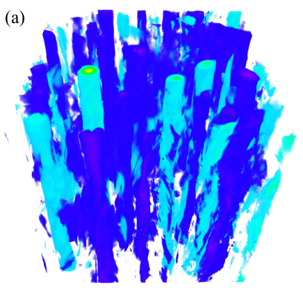
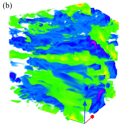
Figure 1: (Color online) (a) Vertical velocity in a $1536^{3}$ simulation of rotating turbulence Mininni and Pouquet (2010). Note the presence of column-like structures. (b) Temperature fluctuations in a $1024^{3}$ simulation of rotating and stratified turbulence with $N/f=2$ Marino et al. (2013). Note the formation of slanted layers, with an angle related to the ratio $N/f$. In the purely stratified case, the layers are horizontal.

When the Reynolds number is large enough the system is in a turbulent state. But even at very large Reynolds numbers, for Fr and Ro small enough, waves are present that affect the turbulent scaling and transport. Thus this system of equations has been extensively studied in numerical simulations as a way to gain a better understanding of atmospheric turbulence in a simplified set up. As mentioned in the introduction, in the atmospheric mesoscales (where the stratification dominates above the rotation, but the dominant regime is quasi-geostrophic and not dominated by inertia-gravity waves), a spectrum of energy compatible with the power law $E(k)\sim k^{-3}$ has been reported. However, a spectrum $E(k)\sim k^{-5/3}$ has also been observed (see, e.g., Cho et al. (1999)), and numerical simulations of Eqs. (1)-(3) have generated results consistent with this power law in the presence of instabilities and small-scale overturning Vincent and Schlatter (1979); Lindborg (2005). Moreover, when overturning is suppressed by dissipation, the spectrum in the simulations becomes steeper. The asymptotic dynamics of this system in the limit of strongly rotating flows generates column-like structures Cambon and Jacquin (1989), while in the limit of strongly stratified vortical motions it seems to consist of quasi-horizontal fluid layers partially decoupled between themselves Liechtenstein et al. (2005) (see Fig. 1). While in the rotating case the direct cascade spectrum of Eqs. (1)-(3) seems to scale as $E(k)\sim k^{-2}$ Cambon and Jacquin (1989); Cambon (2001); Müller and Thiele (2007); Mininni and Pouquet (2010), Billant and Chomaz Billant and Chomaz (2001) argue that in the purely stratified case the vertical characteristic scale $L_{z}$ scales as $U/N$, thus suggesting that the vertical energy spectrum should follow a power law $E(k_{z})\sim N^{2}k_{z}^{-3}$. This behavior was confirmed in numerical simulations Lindborg (2005); Rorai et al. (2014, 2015), where it was also observed that in the purely stratified case the parallel spectrum $E(k_{z})$ is flat for wave numbers smaller than $k_{z}\sim N/U$ Smith et al. (1996); Waite and Bartello (2004); Rorai et al. (2015). As the parallel spectrum dominates over the perpendicular when stratification is sufficiently strong, the isotropic spectrum also follows a law $E(k)\sim k^{-3}$ in the purely stratified case. In the following sections we introduce a decomposition of the flow into slow and fast modes, and the argument of resonant triads, that allow interpretation of some of these results in the direct cascade range, to later consider the case of the inverse cascade.

II.2 Linear modes

In the inviscid and diffusion free limit and in the absence of external forces ($\nu=\kappa={\bf f}=0$), the Boussinesq equations conserve the potential vorticity

$$\frac{D}{Dt}\left(\mbox{\boldmath$\omega$}_{a}\cdot\nabla\theta\right)=0,$$ (7)

where $\mbox{\boldmath$\omega$}_{a}$ is the absolute (total) vorticity in the laboratory frame, $\mbox{\boldmath$\omega$}_{a}=\mbox{\boldmath$\omega$}+2\mbox{\boldmath$\Omega$}$. When rotation and the Brunt-Väisäla frequencies are homogeneous, except for a multiplying prefactor and a constant term, the potential vorticity can be written as

$$P.V.=f\frac{\partial\theta}{\partial z}-N\omega_{z}+\mbox{\boldmath$\omega$}\cdot\nabla\theta.$$ (8)

The conservation of potential vorticity imposes strong constraints on the flow. As a result, solutions to the Boussinesq equations are often decomposed into two groups of modes: inertia-gravity waves with non-zero frequency and zero potential vorticity (also called “fast” modes), and modes with zero frequency and non-zero potential vorticity (also called “slow” modes). By replacing solutions

$$({\bf u},\theta)=\mbox{\boldmath$\psi$}({\bf k})e^{i({\bf k}\cdot{\bf x}+\omega t)},$$ (9)

in the linearized Boussinesq equations, three modes per wave vector ${\bf k}$ can be identified. The two modes with non-zero frequency have dispersion relation Davidson (2013)

$$\omega({\bf k})=\pm\frac{\sqrt{f^{2}k_{\parallel}^{2}+N^{2}k_{\perp}^{2}}}{k},$$ (10)

where the directions parallel and perpendicular are taken with respect to the direction of gravity and of the rotation axis, i.e., $k_{\parallel}=k_{z}$, $k_{\perp}=(k_{x}^{2}+k_{y}^{2})^{1/2}$, and $k=|{\bf k}|$. The group velocity for these modes is

$${\bf c}=\frac{f^{2}-N^{2}}{\omega k^{4}}[{\bf k}\times(k_{\parallel}\hat{z}\times{\bf k})],$$ (11)

and for $f=N$ it can be expected that the role of the waves in the flow dynamics should be less relevant. Also, note that for $f=0$ (the purely stratified case) Eq. (10) reduces to the dispersion relation of internal gravity waves (with the modes with $k_{\perp}=0$ corresponding to the VSHW Smith and Waleffe (2002), which have zero frequency and are thus “slow”). And in the case with $N=0$ (purely rotating flow), the dispersion relation reduces to that of inertial waves (with the slow modes corresponding to 2D modes with $k_{\parallel}=0$).

In the non-linear case, the fields in Fourier space can be expanded in terms of these three modes Waleffe (1993); Babin et al. (1997); Julien et al. (1998); Smith and Waleffe (1999); Bellet et al. (2006); Davidson (2013); Kafiabad and Bartello (2016),

$$({\bf u}_{\bf k},\theta_{\bf k}) = a^{+}({\bf k},t)\mbox{\boldmath$\psi$}^{+}({\bf k})e^{i\omega t}+a^{-}({\bf k},t)\mbox{\boldmath$\psi$}^{-}({\bf k})e^{-i\omega t}$$ (12)

$$+ a^{0}({\bf k},t)\mbox{\boldmath$\psi$}^{0}({\bf k}),$$

where $a^{(\alpha)}({\bf k},t)$ (with $\alpha=+$, $-$, $0$ labeling the three modes) are slowly evolving amplitudes.

II.3 Resonant triads

Fourier transforming the Boussinesq equation, and using the decomposition in Eq. (12), the following equation is obtained Waleffe (1993); Babin et al. (1997); Julien et al. (1998)

$$\frac{da_{\bf k}^{(\alpha)}}{dt} = \sum_{{\bf k}={\bf p}+{\bf q}}C_{\bf kpq}^{\alpha\beta\gamma}a_{\bf p}^{(\beta)}a_{\bf q}^{(\gamma)}e^{i\left(\omega_{\bf p}^{(\beta)}+\omega_{\bf q}^{(\gamma)}-\omega_{\bf k}^{(\alpha)}\right)}$$ (13)

$$+ F_{\bf k}^{(\alpha)}-D_{\bf k}^{(\alpha)},$$

where $C_{\bf kpq}^{\alpha\beta\gamma}$ is a coupling coefficient between modes, $F_{\bf k}^{(\alpha)}$ is the energy injection at wavenumber ${\bf k}$, and $D_{\bf k}^{(\alpha)}$ is the dissipation. The first term on the r.h.s. of this equation corresponds to the non-linear triadic interactions. As nonlinearities in the Boussinesq equations are quadratic, modes are coupled with triads that can exchange energy between themselves while conserving the total energy. The convolution theorem (when the quadratic terms are Fourier transformed) imposes the well known triadic condition

$${\bf k}={\bf p}+{\bf q}.$$ (14)

But the presence of waves imposes an extra condition. Integrating Eq. (13) in one period of the waves, the first term on the r.h.s. of the equation vanishes except when

$$\omega_{\bf k}^{(\alpha)}=\omega_{\bf p}^{(\beta)}+\omega_{\bf q}^{(\gamma)},$$ (15)

which is the so-called resonant triad condition, and selects only the triads with constructive interference between the non-linearly interacting waves.

Waleffe describes the triadic interactions exhaustively for homogeneous turbulence in Waleffe (1992), and the resonant triadic interactions for rapidly rotating flows in Waleffe (1993), where he presents an argument for the two-dimensionalization of rotating flows. His “instability assumption” states that the statistical direction of the energy transfer is determined by the stability of the corresponding elemental triadic interaction. In practice, this results in a preferential transfer of energy towards the modes with zero frequency, although wave turbulence theories cannot explain how energy ultimately reaches these modes Alexakis (2015); di Leoni and Mininni (2016) (as shown in Smith and Lee (2005), near-resonances are needed to explain the efficient transfer of energy to these modes, while non-resonant interactions act reducing this net energy transfer). In spite of these limitations, the argument is succesful in explaining how anisotropy develops. As mentioned in Sec. II.2, for purely rotating flows Eq. (10) reduces to $\omega({\bf k})=\pm fk_{\parallel}/k$, which is the dispersion relation of inertial waves. Energy is then transferred preferentially towards modes with $k_{\parallel}\approx 0$, which correspond to the 2D modes, and if the energy can reach those modes it can be expected to suffer an inverse cascade towards large scales. In purely stratified flows Eq. (10) reduces to $\omega({\bf k})=\pm Nk_{\perp}/k$ (internal gravity waves), and energy then is transferred preferentially towards modes with $k_{\perp}\approx 0$, i.e., to modes with vertical shear. In the former case this explains the formation of structures with small vertical gradients (columns, see Fig. 1), while in the latter case it explains the formation of pancake-like structures (see also Fig. 1).

II.4 Characteristic time scales

In wave turbulence the presence of multiple time scales does not allow for direct estimation of scaling laws in the inertial range as is often done in Kolmogorov theory of turbulence. While in HIT there is only one time scale in the inertial range (the eddy turnover time), in the presence of waves this time scale coexists with the period of the waves, precluding the construction of a unique time scale on dimensional grounds. While in weak wave turbulence regimes this problem can be circumvented (see, e.g., Nazarenko (2011)), in the strong turbulent case the problem persists. Interestingly, one of the first advances towards the construction of phenomenological theories for this kind of systems was also done by Kraichnan, who put forward a theory for the interaction of eddies and Alfvén waves in magnetohydrodynamic turbulence Kraichnan (1965).

Thus, it is important to identify the different time scales relevant in our problem. The decomposition introduced in Sec. II.2 is useful to this end. The first time scale will naturally be proportional to the wave period

$$\tau_{w}({\bf k})=\frac{C_{w}}{\omega({\bf k})}=\frac{C_{w}k}{\sqrt{f^{2}k_{\parallel}^{2}+N^{2}k_{\perp}^{2}}},$$ (16)

where $C_{w}$ is be a dimensionless constant of ${\cal O}$(1) which can be obtained directly from the auto-correlation function of the Fourier modes of the velocity and temperature fields (see di Leoni et al. (2014)).

From Eq. (13) it is to be expected that the fastest time dominates the flow dynamics and the energy transfer. However, although for small enough Ro and Fr the waves are expected to be fast, the period of the waves is not homogeneous in Fourier space as it depends (only) on the direction of ${\bf k}$. Thus, different regions of Fourier space can be dominated by different time scales depending on what mode is the fastest. The period of the waves must then be compared with the eddy turnover time

$$\tau_{nl}(k)=\frac{C_{nl}}{k\sqrt{kE(k)}},$$ (17)

where $C_{nl}$ is another dimensionless constant of ${\cal O}$(1). In principle $\tau_{nl}$ depends on the amplitude of ${\bf k}$ and on its direction in Fourier space, i.e., $\tau_{nl}({\bf k})$, since the energy spectrum in these systems is anisotropic. But for simplicity we will use here the isotropic energy spectrum $E(k)$ to estimate the non-linear time. The condition $\tau_{nl}(k)=\tau_{w}({\bf k})$ for either $N=0$ or $f=0$ yields respectively the Zeman and Ozmidov wave numbers defined in Eqs. (5) and (6). For larger wave numbers, the role of the waves in the non-linear energy transfer can be expected to be negligible.

The last relevant time scale is that of the sweeping of the small eddies by the large scale flow, which becomes the dominant Eulerian decorrelation mechanism as soon as its characteristic time scale becomes the fastest of the three (this often happens at wave numbers smaller than the Zeman and Ozmidov wave numbers, see di Leoni et al. (2014); di Leoni and Mininni (2015); Kraichnan played an important role in highlighting the relevance of this time scale in the case of isotropic and homogeneous turbulence Chen and Kraichnan (1989)). The time to sweep an eddy of size $\sim 1/k$ by a large scale flow with amplitude $U$ is simply

$$\tau_{sw}(k)=\frac{C_{sw}}{Uk},$$ (18)

where $C_{sw}$ is another dimensionless constant of ${\cal O}$(1) that can be determined from the data. These time scales will be very important in the following sections.

Using combinations of these time scales, phenomenological theories for the direct cascade spectrum can be also constructed, following the ideas of Kraichnan Kraichnan (1965). These phenomenological arguments yield spectra compatible with the scaling laws $\sim k^{-2}$ and $\sim k^{-3}$ discussed in the introduction and in Sec. II.1, for solutions of Eqs. (1)-(3), depending on the strength of rotation and stratification considered. For more details see Dubrulle and Valdettaro (1992); Zhou (1995); Billant and Chomaz (2001); Pouquet and Mininni (2010). These time scales, and the results presented in the next two subsections, will be important to elucidate the results of the spatio-temporal analysis in Sec. V.

II.5 Non-resonant range

It can be shown that in the range $1/2\leq N/f\leq 2$ there are no resonant triadic interactions, and therefore all triadic interactions must be near-resonant or non-resonant. In this section we summarize the argument given in Smith and Waleffe (2002). As discussed in Sec. II.3, non-linear interaction of inertia-gravity waves require that the interacting modes ${\bf k}$, ${\bf p}$, and ${\bf q}$ form a triangle, and that the sum of their frequencies give constructive interference. If $N=f$, it is then trivial to see from Eq. (10) that $\omega({\bf k})=\pm N$ for all ${\bf k}$, and then

$$\omega({\bf p})+\omega({\bf q})-\omega({\bf k})=\pm N,\pm 2N,\textrm{or}\pm 3N.$$ (19)

Therefore, the sum of the three frequencies cannot be zero and the condition given by Eq. (15) cannot be fulfilled. Thus, resonant triads do not exist in this case.

In the most general case, Eq. (10) implies that

$$\min\{|\omega({\bf k})|\} = \min\{N,f\},$$ (20)

$$\max\{|\omega({\bf k})|\} = \max\{N,f\}.$$ (21)

Assuming without loss of generality $\omega({\bf k})$, $\omega({\bf p})$, $\omega({\bf q})\geq 0$, to satisfy Eq. (15) we need $2\min\{N,f\}<\max\{N,f\}$. When $\max\{N,f\}=N$, we then need $N/f>2$. When $\max\{N,f\}=f$, then $N/f<1/2$. In these cases there are triads which can satisfy the resonant condition. However, in the range

$$\frac{1}{2}\leq\frac{N}{f}\leq 2,$$ (22)

there is again no triad that can be resonant. Only near-resonances and non-resonant triads are then left to transfer energy between scales.

It is now clear that this range separates two regimes with different behavior. It is expected that outside this range, but in its vicinity, very few resonant triads should be available (thus, resonant triads should play a more relevant role for $N/f\ll 1/2$ or $N/f\gg 2$). For $N/f<1/2$, the first resonant triads that arise (as $N/f$ is decreased) consist of a vertical mode $(0,0,k_{\parallel})$ and of two quasi-horizontal modes ${\bf p}$, ${\bf q}$ with $p_{\perp}=q_{\perp}\gg|k_{\parallel}|,|p_{\parallel}|,|q_{\parallel}|$. Waleffe’s instability assumption then suggests that energy should go from the vertical mode to the perpendicular (slow) modes. Similarly, for $N/f>2$, the first resonant triads that appear as $N/f$ is increased consist of a horizontal mode and two quasi-vertical modes. In this case, the transfer should be expected to occur from the horizontal modes to the quasi-vertical (slow) modes. As with the arguments in Sec. II.3, these arguments suggest that the resonant triads for $N/f<1/2$ tend to bi-dimensionalize the flow (i.e., to make horizontal gradients much larger than vertical gradients, as energy is preferentially transferred towards modes with $k_{\perp}\gg k_{\parallel}$). On the contrary, the resonant triads for $N/f>2$ tend to unidimensionalize the flow (i.e., to make vertical gradients much larger than horizontal gradients, or $k_{\parallel}\gg k_{\perp}$). An illustration of this can be seen in Fig. 1, which shows column-like structures in the vertical velocity in a simulation with pure rotation, and pancake-like structures in a simulation with rotation and stratification.

II.6 Quasi-geostrophic equation

Simulations in the range $1/2\leq N/f\leq 2$ show that at scales larger than the forced scales QG modes dominate the dynamics Smith et al. (1996), in agreement with the theoretical prediction that resonant triads are not available in this region of parameter space. As in other limits of geophysical flows, this can be used to derive a reduced system of equations. Although the QG approximation is often derived in the limit of very small Froude number and moderate rotation (of interest in atmospheric sciences), Smith and Waleffe Smith et al. (1996); Smith and Waleffe (2002) showed that the QG equations can be also obtained for moderate values of $N/f$, which can be of interest for some oceanographic applications. Here we briefly summarize their derivation.

If only modes with zero frequency are excited, in the inviscid and unforced case Eq. (13) can be written as

$$\frac{da_{\bf k}^{0}}{dt}=\sum_{{\bf k}={\bf p}+{\bf q}}C_{{\bf k}{\bf p}{\bf q}}a_{\bf p}^{0}a_{\bf q}^{0},$$ (23)

where Smith and Waleffe (2002)

$$C_{{\bf k}{\bf p}{\bf q}}\equiv C_{{\bf k}{\bf p}{\bf q}}^{000}=$$ (24)

$$\frac{iN({\bf p}\times{\bf q})\cdot\hat{z}\left[f^{2}(q_{\parallel}^{2}-p_{\parallel}^{2})+N^{2}(q_{\perp}^{2}-p_{\perp}^{2})\right]}{\left[(f^{2}k_{\parallel}^{2}+N^{2}k_{\perp}^{2})(f^{2}p_{\parallel}^{2}+N^{2}p_{\perp}^{2})(f^{2}q_{\parallel}^{2}+N^{2}q_{\perp}^{2})\right]^{1/2}}.$$

The triadic condition in Eq. (14) implies that $({\bf p}\times{\bf q})\cdot\hat{z}=({\bf q}\times{\bf k})\cdot\hat{z}=({\bf k}\times{\bf q})\cdot\hat{z}$, that is, that the $C_{{\bf k}{\bf p}{\bf q}}$ coupling coefficients are cyclic permutations of the wave vectors multiplied by $f^{2}(q_{\parallel}^{2}-p_{\parallel}^{2})+N^{2}(q_{\perp}^{2}-p_{\perp}^{2})$. It then follows that

$$C_{{\bf k}{\bf p}{\bf q}}+C_{{\bf p}{\bf q}{\bf k}}+C_{{\bf q}{\bf p}{\bf k}}=0,$$ (25)

and

$$(f^{2}k_{\parallel}^{2}+N^{2}k_{\perp}^{2})C_{{\bf k}{\bf p}{\bf q}}+(f^{2}p_{\parallel}^{2}+N^{2}p_{\perp}^{2})C_{{\bf p}{\bf q}{\bf k}}+$$

$$(f^{2}q_{\parallel}^{2}+N^{2}q_{\perp}^{2})C_{{\bf q}{\bf p}{\bf k}}=0,$$ (26)

which convey two conservation laws as discussed below.

Taking $\psi_{\bf k}=-Na_{\bf k}^{0}/(k\omega_{\bf k})$, and Fourier transforming Eq. (23) into real space, we obtain

$$\left(\frac{\partial}{\partial t}+{\bf v}\cdot\nabla\right)\left(\nabla_{\perp}^{2}+\frac{f^{2}}{N^{2}}\frac{\partial^{2}}{\partial z^{2}}\right)\psi({\bf x},t)=0,$$ (27)

where $\nabla_{\perp}^{2}=\partial_{x}^{2}+\partial_{y}^{2}$, ${\bf v}=\hat{z}\times\nabla\psi$, and $\theta=-(f/N)\partial_{z}\psi$. This is the quasi-geostrophic equation, which conserves two quadratic invariants: the total energy

$$E=\frac{1}{2}\left<\left|\nabla_{\perp}\psi\right|^{2}+\frac{f^{2}}{N^{2}}\left(\frac{\partial\psi}{\partial z}\right)^{2}\right>,$$ (28)

with $\nabla_{\perp}=\partial_{x}\hat{x}+\partial_{y}\hat{y}$, and the potential enstrophy

$$F=\frac{1}{2}\left<\left(\nabla_{\perp}^{2}\psi+\frac{f^{2}}{N^{2}}\frac{\partial^{2}\psi}{\partial z^{2}}\right)^{2}\right>.$$ (29)

As in the 2D case studied by Kraichnan Kraichnan (1967), the existence of two invariants in this case also allows for the development of an inverse cascade of energy Charney (1971); Herring (1988); Vallgren and Lindborg (2010). This result will be important in the following sections, as we will see that in the range $1/2\leq N/f\leq 2$, rotating and stratified turbulence can develop a very efficient inverse cascade of energy, with a prevalence of slow modes satisfying QG scaling.

III Inverse cascades

To discuss previous results in inverse cascades, and to analyze the new results in this paper, we will use isotropic and anisotropic spectra and fluxes. We thus begin by defining the isotropic kinetic energy spectrum, which is computed in numerical simulations as

$$E_{V}(k)=\frac{1}{2}\sum_{k\leq|{\bf k}|<k+1}|{\bf u}({\bf k})|^{2},$$ (30)

i.e., as the energy in spherical shells of width $\Delta k=1$ in Fourier space. An equivalent definition is obtained for the power spectrum of temperature fluctuations $E_{P}(k)$ (sometimes also called the potential energy spectrum) replacing $|{\bf u}({\bf k})|^{2}$ by $|\theta({\bf k})|^{2}$, and the total energy spectrum is then simply constructed as $E(k)=E_{V}(k)+E_{P}(k)$. The kinetic energy spectrum can be further decomposed into the kinetic energy in horizontal fluctuations and in vertical fluctuations, $E_{V}(k)=E_{\perp}(k)+E_{z}(k)$, where $E_{\perp}(k)$ is the energy in the $x$ and $y$ components of the velocity field, and $E_{z}(k)$ is the energy in $u_{z}$.

As the flows we consider are anisotropic, it is useful to define the axisymmetric kinetic energy spectrum

$$e_{V}(k_{\perp},k_{\parallel})=\frac{1}{2}\sum_{\begin{subarray}{c}k_{\perp}\leq|{\bf k}\times\hat{\bf z}|<k_{\perp}+1\\ k_{\parallel}\leq k_{z}<k_{\parallel}+1\end{subarray}}|{\bf u}({\bf k})|^{2},$$ (31)

The axisymmetric kinetic energy spectrum in Eq. (31) is such that the total kinetic energy in 2D modes is $E_{2D}=\sum_{k_{\perp}}e_{V}(k_{\perp},k_{\parallel}=0)$. As a result, we will refer to $e_{V}(k_{\perp},k_{\parallel}=0)$ as the kinetic energy spectrum of the 2D modes. As for the isotropic spectra, we can decompose the axisymmetric kinetic energy spectrum into $e_{V}(k_{\perp},k_{\parallel})=e_{\perp}(k_{\perp},k_{\parallel})+e_{z}(k_{\perp},k_{\parallel})$, and we can write the axisymmetric total energy spectrum as $e(k_{\perp},k_{\parallel})=e_{V}(k_{\perp},k_{\parallel})+e_{P}(k_{\perp},k_{\parallel})$. Note in Eqs. (30) and (31) we use sums as we are considering the discrete Fourier transform for a triple $2\pi$-periodic spatial domain. In the most general case these sums are replaced by integrals.

To quantify energy scaling in the parallel and perpendicular directions, reduced perpendicular and parallel spectra can then be defined from the axisymmetric energy spectrum as, e.g., for the total energies:

$$E(k_{\perp})=\sum_{k_{\parallel}}e(k_{\perp},k_{\parallel}),$$ (32)

and

$$E(k_{\parallel})=\sum_{k_{\perp}}e(k_{\perp},k_{\parallel}).$$ (33)

Identification of inverse cascades requires not only the study of the growth of energy in these spectra for small wave numbers, but also quantification of negative flux of energy in a range of wave numbers. To this end we can define anisotropic transfer functions associated with each energy spectra $E(k)$, $E(k_{\perp})$, and $E(k_{\parallel})$ respectively as

$$T(k)=-\sum_{k\leq|{\bf k}|<k+1}t({\bf k}),$$ (34)

$$T(k_{\perp})=-\sum_{k_{\perp}\leq|{\bf k}\times\hat{z}|<k_{\perp}+1}t({\bf k}),$$ (35)

$$T(k_{\parallel})=-\sum_{k_{\parallel}\leq k_{z}<k_{\parallel}}t({\bf k}),$$ (36)

where $t({\bf k})={\bf u}^{\star}({\bf k})\cdot\widehat{({\bf u}\cdot\nabla{\bf u})}+\theta^{\star}({\bf k})\widehat{({\bf u}\cdot\nabla\theta)}+c.c.$, where ^⋆ and $c.c.$ denotes complex conjugate, and the superscript $\widehat{}$ denotes the Fourier transform. From these functions anisotropic fluxes are then defined as follows:

$$\Pi(k)=-\sum_{k^{\prime}=0}^{k}T(k^{\prime}),$$ (37)

$$\Pi(k_{\perp})=-\sum_{k_{\perp}^{\prime}=0}^{k_{\perp}}T(k^{\prime}_{\perp}),$$ (38)

$$\Pi(k_{\parallel})=-\sum_{k^{\prime}_{\parallel}=0}^{k_{\parallel}}T(k^{\prime}_{\parallel}).$$ (39)

These fluxes measure energy per unit of time that goes in Fourier space respectively across spheres with radius $k$, across cylinders with radius $k_{\perp}$, and across planes with height $k_{\parallel}=$ constant.

III.1 Rotating case

In the purely rotating case with moderate Rossby number, the preferential transfer of energy towards 2D modes results in the development of an inverse cascade which shares some similarities with the inverse cascade originally proposed by Kraichnan. By now evidence of this inverse cascade has been found in numerical simulations in finite domains Sen et al. (2012) and in experiments Campagne et al. (2014). There is still a controversy of whether this inverse cascade can take place in infinite domains and for very small Rossby numbers, for more details see, e.g., Ref. Cambon et al. (2004).

An interesting property of the inverse cascade of energy in this case is that changes in the forcing function or in the dominant time scale can generate large differences in the scaling of the energy spectrum (see Sen et al. (2012)). In particular, the anisotropy of the forcing seems to play an important role in setting the shape of the inverse cascade energy spectrum. As an illustration, Fig. 2 shows the reduced perpendicular spectrum $E(k_{\perp})$ and the horizontal kinetic energy spectrum of 2D modes $e_{\perp}(k_{\perp},k_{\parallel}=0)$ for two simulations of rotating turbulence forced at small scales.

The two simulations, which have $\textrm{Re}\approx 400$ and $\textrm{Ro}=0.045$, were continued for over 250 turnover times, and both have $k_{\Omega}\gtrsim 1800$, much larger than the largest resolved wave number (i.e., all wave numbers in the simulation are dominated by rotation). The difference between these two simulations is in the isotropy (or anisotropy) of the forcing function. While in both cases a random forcing is used, in one case energy is injected isotropically in all modes in the spherical shell with $k=k_{F}\approx 40$, while in the other energy is injected mostly in the modes (in the same spherical shell) that are close to the $k_{\perp}$ plane (i.e., preferentially into modes with small $k_{\parallel}$, or the 2D modes). A detailed analysis of anisotropic fluxes in Sen et al. (2012) shows that while in the former case this results in a transfer of energy from the 3D modes to the 2D modes which then drive the inverse cascade, in the latter case the energy that is fed directly into the 2D modes undergoes an inverse cascade and then feeds the 3D modes once the energy accumulates at the largest available scale. Eventually, at sufficiently long times the energy accumulates in both cases at the smallest available wave number, $k=1$, and energy then leaks from these modes towards the 3D modes. The behavior of the systems at long times also depends on whether large-scale friction is used or not.

Before this time, the changes in the energy fluxes (and in the coupling between 2D and 3D modes) result in two different scaling laws, with one case displaying spectra $E(k_{\perp})$ and $e_{\perp}(k_{\perp},k_{\parallel}=0)\sim k_{\perp}^{-3}$, and the other with spectra $E(k_{\perp})$ and $e_{\perp}(k_{\perp},k_{\parallel}=0)$ compatible with $\sim k_{\perp}^{-5/3}$. These two scaling laws can be explained using phenomenological arguments similar to those used by Kraichnan Sen et al. (2012). In the latter case, in which energy is injected directly into the 2D modes, and in which little energy goes into the 2D modes from the 3D modes, we can assume that the inverse cascade in the slow 2D modes is dominated by the turnover time $\tau_{\perp}\sim l_{\perp}/u_{\perp}$ (where $l_{\perp}$ is a characteristic perpendicular length, and $u_{\perp}$ is the 2D r.m.s. velocity at that length scale). With only one relevant timescale, Kraichnan phenomenology for the inverse cascade tells us that the energy flux in the 2D modes goes as

$$\Pi_{2D}\sim\frac{u_{\perp}^{2}}{\tau_{\perp}}\sim\frac{u_{\perp}^{3}}{l_{\perp}},$$ (40)

which results in a $\sim\epsilon^{2/3}k_{\perp}^{-5/3}$ spectrum for the 2D modes (assuming the energy injection rate at all modes $\epsilon$ and the 2D energy flux $\Pi_{2D}$ are proportional).

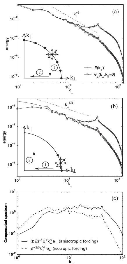
Figure 2: (a) Reduced perpendicular energy spectrum $E(k_{\perp})$ and perpendicular kinetic energy in the 2D modes $e_{\perp}(k_{\perp},k_{\parallel}=0)$ in a simulation of rotating turbulence forced at small scales with random isotropic forcing. The inset illustrates how the forcing acts over the spherical shell in Fourier space; energy is transfered first towards the 2D modes and then develops an inverse cascade. (b) Same for a simulation with anisotropic forcing. The inset illustrates how the energy that is injected directly into the 2D modes has an inverse cascade, and then it is transferred towards 3D modes as accumulation of energy at large scales saturates. In both figures power laws are shown as a reference (see Sen et al. (2012) for more details). (c) Energy spectrum of 2D motions $e_{\perp}(k_{\perp},k_{\parallel}=0)$ compensated by $\epsilon^{2/3}k_{\perp}^{-5/3}$ in the run with random isotropic forcing, and by $\epsilon\Omega U^{-2}k_{\perp}^{-3}$ (where $U$ is the r.m.s. velocity at the forcing scale) in the run with anisotropic forcing. The amplitudes of both spectra when compensated (i.e., the “Kolmogorov constants”) are found to be of order unity.

On the other hand, if the forcing is isotropic and energy goes from the 3D modes to the 2D modes, interactions with the 3D modes cannot be neglected. Besides the slow turnover time $\tau_{\perp}$, we now have to consider the time scale of the waves (which is the fastest time scale for many of the 3D modes), and which we can estimate as $\tau_{\Omega}\sim 1/\Omega$. Using Kraichnan phenomenology for interactions of waves and eddies Kraichnan (1965), we can assume that the non-linear transfer will be slowed down by a factor proportional to the Rossby number, i.e., to the ratio of time scales between the wave period and some non-linear turnover time. Then,

$$\Pi_{2D}\sim\left(\frac{u_{\perp}^{2}}{\tau_{nl}}\right)\left(\frac{\tau_{\Omega}}{\tau_{nl}}\right)\sim\frac{u_{\perp}^{2}}{\Omega\tau_{nl}^{2}}.$$ (41)

Assuming again $\Pi_{2D}$ is proportional to $\epsilon$, and if the turnover time in the above expression is built upon the velocity at the forcing scale $U$ (i.e., $\tau_{nl}\sim l_{\perp}/U$, assuming most of the energy in the 2D modes comes directly from the 3D forced modes), this relation results in a spectrum $\sim\epsilon\Omega U^{-2}k_{\perp}^{-3}$ for the 2D modes Sen et al. (2012). Figure 2(c) shows the spectrum of 2D modes in the simulations with isotropic and with anisotropic random forcing compensated by their corresponding expressions. In both cases, the compensated spectra have amplitudes close to unity in the inverse cascade range. In comparison, the Kolmogorov constant for the classical 2D inverse cascade is in the range $\approx 5.5$ – $7$ Paret and Tabeling (1997), although in some experiments its value was also reported to depend on the rate at which energy was extracted at large scales Sommeria (1986).

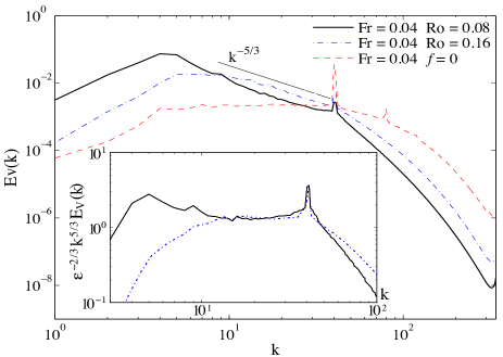
Figure 3: (Color online) Isotropic kinetic energy spectrum in a $1024^{3}$ simulation of a stably stratified flow ($f=0$, i.e., without rotation), and in two $1024^{3}$ simulations of rotating and stratified flows with the same Froude number and different Rossby numbers (see Marino et al. (2014) for details). Note the growth of energy at wave numbers smaller than the forcing wavenumber $k_{F}\approx 40$ in the two latter simulations, and the flat spectrum at the same wave numbers in the former case. A $\sim k^{-5/3}$ power law is indicated as a reference. The inset shows the spectrum of the two simulations with rotation and stratification compensated by $\epsilon^{2/3}k^{-5/3}$. The amplitude of the compensated spectra in the flat range (i.e., the “Kolmogorov constant”) is $\approx 1.3$. Note this value is smaller than the Kolmogorov constant for the classical 2D inverse cascade $\approx 5.5$ – $7$ Paret and Tabeling (1997).

III.2 Stratified case

A detailed study of the effect of the forcing on the development and growth of large scales in stratified flows (as well as in rotating and stratified flows) is still partially missing. For the sake of simplicity, from here on we will consider either isotropic forcing functions, or Taylor-Green forcing which does not inject energy directly into 2D modes, and which for the rotating case was shown to give an inverse cascade with the same scaling as isotropic forcing Sen et al. (2012).

Figure 3 shows the isotropic energy spectrum in a $1024^{3}$ simulation of a purely stratified flow with $\textrm{Re}\approx 1000$ and $\textrm{Fr}=0.04$ ($f=0$ as there is no rotation, and the Ozmidov wavenumber is $k_{\textrm{Oz}}\approx 510$, larger than the largest resolved wave number in the simulation $1024/3\approx 341$; see Marino et al. (2013, 2014) for more details). The flow is forced at $k_{F}\approx 40$ so there is room at small wave numbers for an inverse cascade to develop. Instead, what we observe is that energy grows at wave numbers $k<k_{F}$, but with a flat spectrum in this range.

In the purely stratified case there is growth of energy at large scales as energy piles up into VSHW, i.e., modes for the horizontal velocity with $k_{\perp}\approx 0$ and with strong vertical gradients Smith and Waleffe (2002). However, this growth is not accompanied by a negative constant energy flux in a wide range of scales as expected for an inverse cascade Waite and Bartello (2004, 2006); Marino et al. (2014). Instead, the isotropic energy flux tends to be small at large scales (small wave numbers), while the parallel energy flux becomes negative and the perpendicular energy flux becomes positive Marino et al. (2014). In other words, the growth of energy at large scales is not the result of a self-similar cascade but rather of a very strong anisotropization of the flow. Candidates for the generation of the VSHW include resonant triads Smith and Waleffe (2002) and absorption of waves by critical layers di Leoni and Mininni (2015).

III.3 Rotating and stratified case

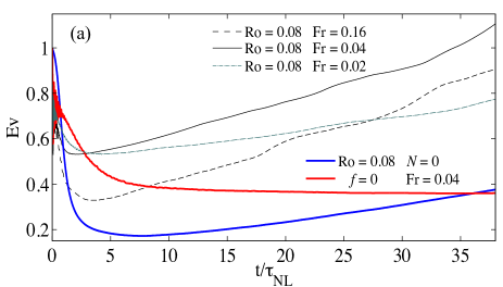
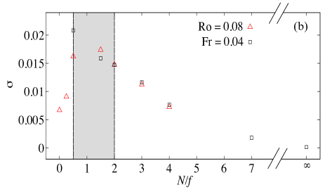
Figure 4: (Color online) (a) Kinetic energy as a function of time in several $1024^{3}$ simulations of rotating and stratified turbulence. The thick lines correspond to purely rotating or purely stratified simulations. The thin lines correspond to rotating and stratified runs. The two runs in the range $1/2\leq N/f\leq 2$ have the fastest growth of $E_{V}(t)$. (b) Average in time growth speed $\sigma=dE_{V}/dt$ of the kinetic energy as as a function of $N/f$ for two sets of simulations: one with fixed $\textrm{Ro}=0.08$ and varying Fr, and another with fixed $\textrm{Fr}=0.04$ and varying Ro. The range $1/2\leq N/f\leq 2$, which displays the fastest growth, is indicated by the gray shading (see Marino et al. (2013) for more details).

As explained in the introduction and in Sec. II, the inverse Prandtl ratio $N/f$ is expected to play an important role controlling the different regimes of the inverse cascade in rotating and stratified flows. At this point, we know that while in the purely rotating case ($N/f\to 0$) there is an inverse cascade, in the purely stratified case ($N/f\to\infty$) there is none. Although a priori a monotonous decrease of the strength of the inverse cascade could be expected between these two limit cases, the non-monotonicity in the strength of the resonant interactions with $N/f$ suggests there can be a distinct behavior in the range $1/2\leq N/f\leq 2$.

This problem was considered in detail in Marino et al. (2013), where a parametric study of the inverse cascade was done varying $N/f$ in a large set of numerical simulations with spatial resolutions with up to $1024^{3}$ grid points and Reynolds numbers up to $\approx 1000$. Figure 3 shows the isotropic kinetic energy spectrum for two $1024^{3}$ runs of rotating and stratified flows forced at small scales with fixed Froude number ($\textrm{Fr}=0.04$) and two different Rossby numbers ($\textrm{Ro}=0.08$ and $0.16$). Unlike the purely stratified case, both simulations display growth of energy at large scales, negative energy flux (not shown here), and a spectrum compatible with a $\sim k^{-5/3}$ power law at small scales. The simulation with $\textrm{Ro}=0.08$ shows a larger peak of the energy spectrum, taking place at smaller wave numbers ($k\approx 4$). As both spectra are displayed at the same time, this indicates that the inverse cascade is faster in this simulation (which has $N/f=2$), compared with the simulation with $\textrm{Ro}=0.16$ which has $N/f=4$.

Table 1: Parameters of the $512^{3}$ simulations in Secs. IV and V: $N$ is the Brunt-Väisäla frequency, $f$ is the Coriolis frequency, Fr is the Froude number, Ro is the Rossby number, $\epsilon$ is the energy injection rate, $k_{\textrm{Oz}}$ is the Ozmidov wavenumber, and $k_{\Omega}$ is the Zeman wavenumber (the maximum resolved wavenumber in $512^{3}$ runs is $512/3\approx 170$).

Run	$N$	$f$	Fr	Ro	$\epsilon$	$k_{\textrm{Oz}}$	$k_{\Omega}$
$1$	$0.25$	1	$0.8$	$0.2$	$0.01$	$1.2$	10
$2$	$0.5$	1	$0.4$	$0.2$	$0.01$	$3.5$	10
$3$	$2$	1	$0.1$	$0.2$	$0.01$	28	10
$4$	$5$	1	$0.04$	$0.2$	$0.01$	112	10
$5$	$0.5$	2	$0.3$	$0.075$	$0.005$	5	40
$6$	$1$	1	$0.2$	$0.2$	$0.02$	7	7
$7$	$4$	8	$0.08$	$0.04$	$0.007$	95	270
$8$	$8$	4	$0.05$	$0.1$	$0.003$	413	146

The results of the detailed parametric study of the effect of varying $N/f$ on the inverse cascade is summarized in Fig. 4. Figure 4(a) shows the kinetic energy as a function of time, $E_{V}(t)$, for several simulations with varying Ro and Fr numbers. The simulations are forced at small scales and started from random initial conditions at wave numbers $k>k_{F}$ (where $k_{F}$ is the forcing wavenumber). First the energy decays as the system develops a turbulent spectrum, and after $\approx 5$ turnover times two regimes can be observed. In the simulation without rotation ($f=0$), $E_{V}(t)$ remains approximately constant. In the simulation without stratification ($N=0$), energy grows monotonously in time. The same happens in the rotating and stratified cases, but the two simulations with $N/f=1/2$ and $N/f=2$ display the fastest growth of the energy.

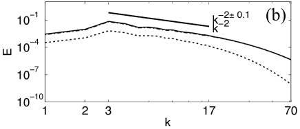
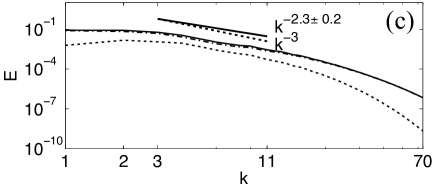
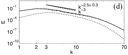
Figure 5: Detail of the direct cascade inertial range in the isotropic spectra of kinetic energy $E_{V}$, power spectrum of temperature fluctuations $E_{P}$, and total energy $E$, in several $512^{3}$ simulations of rotating and stratified turbulence, all forced at $k_{F}\approx 3$ and with $\textrm{Ro}\approx 0.2$. (a) $\textrm{Fr}=0.8$, $N/f=1/4$ (run 1), (b) $\textrm{Fr}=0.4$, $N/f=1/2$ (run 2), (c) $\textrm{Fr}=0.1$, $N/f=2$ (run 3), and (d) $\textrm{Fr}=0.04$, $N/f=5$ (run 4). Several power laws are shown as references.

A parametric study of this growth speed as a function of $N/f$ for multiple runs is shown in Fig. 4(b). Two sets of simulations are shown, one with fixed Ro and varying $N/f$ by varying the Fr number, and another with fixed Fr and varying Ro. In all cases, simulations with $1/2\leq N/f\leq 2$ display the fastest growth of the energy. In Marino et al. (2013) it was shown that this growth corresponds to a growth of the energy in 2D modes at large scales, and that it is caused by an inverse energy cascade with constant (and negative) energy flux which also takes maximum values in the range $1/2\leq N/f\leq 2$. In Marino et al. (2013) it was thus speculated that the larger efficiency of the inverse cascade in this range was associated with the absence of resonant interactions and the prevalence of QG behavior in this region of parameter space. In the rest of this paper we will consider new simulations and analysis to confirm this is indeed the case.

IV Quasi-geostrophic behavior

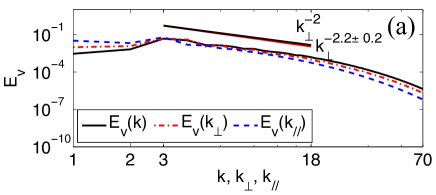
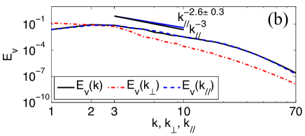
Figure 6: (Color online) Detail of the direct cascade inertial range in the isotropic spectrum of kinetic energy $E_{V}(k)$, reduced perpendicular spectrum of kinetic energy $E_{V}(k_{\perp})$, and reduced parallel spectrum of kinetic energy $E_{V}(k_{\parallel})$, for two $512^{3}$ simulations of rotating and stratified turbulence forced at $k_{F}\approx 3$ with $\textrm{Ro}\approx 0.2$. (a) $\textrm{Fr}=0.8$, $N/f=1/4$ (run 1), and (b) $\textrm{Fr}=0.04$, $N/f=5$ (run 4). Several power laws are shown as references.

For the analysis in this section and in the next, we performed a new set of simulations of rotating and stratified turbulence. As in Sec. V we will perform a spatio-temporal analysis of the data to extract the strength of the waves (which requires storage of the data with very high cadence in time), we will only be able to consider moderate spatial resolutions. Therefore, while simulations in the previous sections had spatial resolutions of $1024^{3}$ grid points or larger, simulations in the next two sections will consist of two large datasets of runs with $256^{3}$ and $512^{3}$ grid points. As in the previous sections, we will explore parameter space by considering multiple values of Fr, and for each of these values we will vary Ro to explore the effect of changing $N/f$. Overall, we performed 15 simulations with $256^{3}$ grid points with $\textrm{Re}\approx 800$, $0.02\lesssim\textrm{Fr}\lesssim 1.8$ ($0.1\leq N\leq 10$), $0.04\lesssim\textrm{Ro}\lesssim 0.3$ ($0.6\leq N\leq 8$), and $0.1\lesssim N/f\lesssim 10$, and one simulation without rotating nor stratification ($f=N=0$). We also performed 8 simulations with $512^{3}$ grid points with $\textrm{Re}\approx 1500$, $0.05\lesssim\textrm{Fr}\lesssim 0.8$, $0.04\lesssim\textrm{Ro}\lesssim 0.2$, and $0.25\lesssim N/f\lesssim 5$. The parameters and characteristic wave numbers for these 8 simulations are given in detail in Table 1.

Also, as resolution in these simulations is limited, we forced the flow at much larger scales leaving very little room for the growth of energy at large scales. We thus use Taylor-Green forcing Mininni et al. (2008) acting at $k_{F}=3\sqrt{2}\approx 3$. Large scale forcing is required as one of our goals will be to identify the role of the waves at small scales, but it will force us to complement the results in these sections with the results in the previous sections where time resolution was not as good, but the inverse cascade ranges were better resolved. To study both ranges separately is a common practice in geophysical fluid dynamics due to constraints in computing power, as only very recently simulations were able to resolve dual cascades in a unique simulation at very high resolution Marino et al. (2015a).

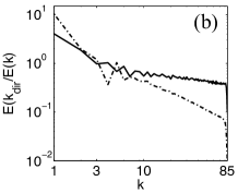
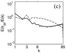
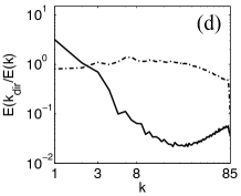
Figure 7: Ratio of the spectra $E(k_{\perp})/E(k)$ (solid) and $E(k_{\parallel})/E(k)$ (dash-dotted) for several $256^{3}$ simulations of rotating and stratified turbulence forced at $k_{F}\approx 3$ with $\textrm{Ro}\approx 0.2$. (a) $\textrm{Fr}=0.8$, $N/f=1/4$, (b) $\textrm{Fr}=0.4$, $N/f=1/2$, (c) $\textrm{Fr}=0.1$, $N/f=2$, and (d) $\textrm{Fr}=0.04$, $N/f=5$.

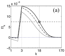
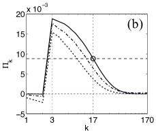
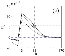
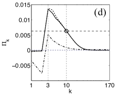
Figure 8: Isotropic energy flux $\Pi(k)$ (solid), perpendicular energy flux $\Pi(k_{\perp})$ (dashed), and parallel energy flux $\Pi(k_{\parallel})$ (dash-dotted) in several $512^{3}$ simulations of rotating and stratified turbulence forced at $k_{F}=3$ with $Ro\approx 0.2$. From left to right and top to bottom: (a) $\textrm{Fr}=0.8$, $N/f=1/4$ (run 1), (b) $\textrm{Fr}=0.4$, $N/f=1/2$ (run 2), (c) $\textrm{Fr}=0.1$, $N/f=2$ (run 3), and (d) $\textrm{Fr}=0.04$, $N/f=5$ (run 4). The straight lines and the circles indicate the wave number at which the flux drops to $1/2$ of its value at the forcing wave number $k_{F}\approx 3$. Note that the largest negative isotropic and perpendicular fluxes (for $k<k_{F}$) are obtained in the case with $N/f=2$. The simulation with $N/f=5$ has negative parallel flux, but negligible isotropic and perpendicular inverse fluxes at large scales.

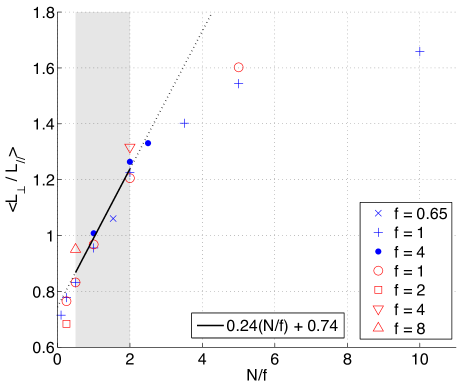
Figure 9: (Color online) Ratio of the perpendicular to parallel integral scales $\left<L_{\perp}/L_{\parallel}\right>$ (averaged over time in the turbulent steady state) as a function of $N/f$ for several $256^{3}$ and $512^{3}$ simulations of rotating and stratified turbulence with varying Ro and Fr numbers. The range with no resonant interactions, $1/2\leq N/f\leq 2$, is indicated by the gray shading. In this range, a linear fit of $\left<L_{\perp}/L_{\parallel}\right>$ as a function of $N/f$ (expected from quasi-geostrophy) is shown as a reference.

Figure 5 shows a detail, in the vicinity of the inertial range, of the isotropic energy spectrum $E(k)$ for four $512^{3}$ runs with $\textrm{Ro}\approx 0.2$ and varying Fr (and therefore, varying $N/f$). Power laws $\sim k^{-2}$ and $\sim k^{-3}$ are shown as references. Also as a reference we present a best fit to a power law in the range of scales $k\in[k_{F},k_{1/2}]$, where $k_{1/2}$ is the wave number at which the energy flux drops to $1/2$ of its value at the injection scale, i.e., $\Pi(k_{1/2})=\Pi(k_{F})/2$. This fit is not intended to claim a specific power law followed by the inertial range, as the value of $1/2$ used to define the drop in the flux is arbitrary, but rather to illustrate that as $N/f$ increases, the energy spectrum becomes steeper, going from the behavior expected for a purely rotating flow ($\sim k^{-2}$) to that of a purely stratified flow ($\sim k^{-3}$). This can be also understood from the values of the Zeman and Ozmidov wavenumbers in Table 1. In Fig. 5(a), which corresponds to run 1, $k_{\textrm{Oz}}\approx 1.2$ and all intermediate wave numbers are dominated by rotation, at least until $k_{\Omega}\approx 10$. As the Brunt-Väisäla frequency is increased, the Ozmidov wavenumber also increases, and more scales are dominated by both rotation and stratification. The energy spectrum of run 4, shown in Fig. 5(d), corresponds to $k_{\textrm{Oz}}\approx 112$ and $k_{\Omega}\approx 10$. Thus, in this case stratification is dominant at all scales. Also, note that a small growth of energy at wave numbers $k<k_{F}$ can be observed in some of these runs. Although the scale separation at large scales (small wave numbers) in these runs is small to study the inverse cascade, inverse transfer can be observed, as will be also shown in the energy fluxes.

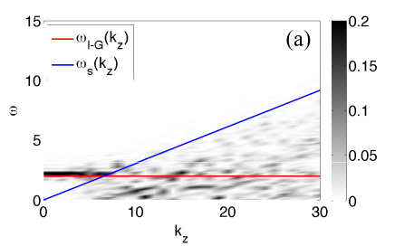
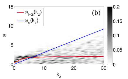
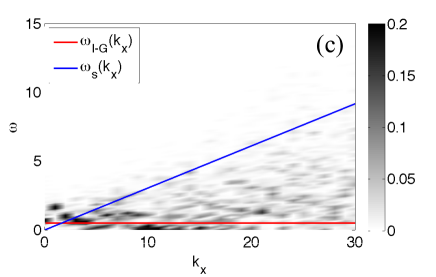
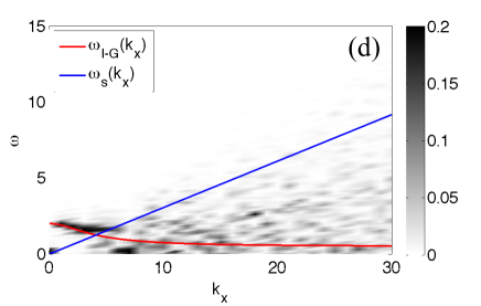
Figure 10: (Color online) Spatio-temporal power spectra $|u_{x}|^{2}(k_{x},k_{y},k_{z},\omega)$ and $|u_{z}|^{2}(k_{x},k_{y},k_{z},\omega)$ for a $512^{3}$ simulation of rotating and stratified turbulence with $\textrm{Fr}=0.3$, $\textrm{Ro}=0.075$ ($N/f=1/4$, run 5 in Table 1). Two-dimensional slices of each four-dimensional spectrum are shown by fixing two components of the wave vector. (a) $|u_{x}|^{2}(k_{x}=0,k_{y}=0,k_{z},\omega)$, (b) $|u_{x}|^{2}(k_{x}=3,k_{y}=0,k_{z},\omega)$, (c) $|u_{z}|^{2}(k_{x},k_{y}=0,k_{z}=0,\omega)$, and (d) $|u_{z}|^{2}(k_{x},k_{y}=0,k_{z}=3,\omega)$. The solid lines indicate the dispersion relation of inertia-gravity waves, $\omega_{\textrm{I-G}}({\bf k})$, and of sweeping, $\omega_{s}({\bf k})$.

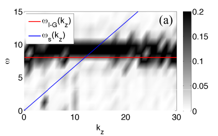
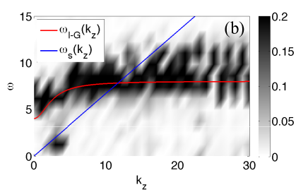
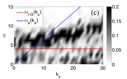
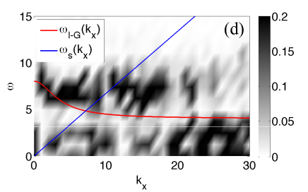
Figure 11: (Color online) Spatio-temporal power spectra $|u_{x}|^{2}(k_{x},k_{y},k_{z},\omega)$ and $|u_{z}|^{2}(k_{x},k_{y},k_{z},\omega)$ for a $512^{3}$ simulation of rotating and stratified turbulence with $\textrm{Fr}=0.08$, $\textrm{Ro}=0.04$ ($N/f=1/2$, run 7 in Table 1). Two-dimensional slices of each four-dimensional spectrum are shown by fixing two components of the wave vector. (a) $|u_{x}|^{2}(k_{x}=0,k_{y}=0,k_{z},\omega)$, (b) $|u_{x}|^{2}(k_{x}=3,k_{y}=0,k_{z},\omega)$, (c) $|u_{z}|^{2}(k_{x},k_{y}=0,k_{z}=0,\omega)$, and (d) $|u_{z}|^{2}(k_{x},k_{y}=0,k_{z}=3,\omega)$. The solid lines indicate the dispersion relation of inertia-gravity waves, $\omega_{\textrm{I-G}}({\bf k})$, and of sweeping, $\omega_{s}({\bf k})$.

Figure 6 shows the isotropic and reduced parallel and perpendicular spectra of the kinetic energy for two of the simulations shown in Fig. 5. Again, power laws and best fits to the spectrum are shown as references. While in the inertial range for the case with $N/f=1/4$ the reduced perpendicular spectrum $E(k_{\perp})$ is closer to the isotropic spectrum $E(k)$, in the case with $N/f=5$ the reduced parallel spectrum $E(k_{\parallel})$ is closer to $E(k)$. In other words, in the case with stronger rotation most of the energy seems to accumulate near modes with $k_{\parallel}\approx 0$, while in the case with stronger stratification energy accumulates near modes with $k_{\perp}\approx 0$.

This is further illustrated in Fig. 7, which shows the ratios $E(k_{\perp})/E(k)$ and $E(k_{\parallel})/E(k)$ for several simulations with varying $N/f$. For $N/f<1$ and for $k>k_{F}$, the ratio $E(k_{\perp})/E(k)$ is of order one in a wide range of wave numbers, while $E(k_{\parallel})/E(k)$ decreases rapidly with increasing wave number. On the other hand, for $N/f>1$ the ratio $E(k_{\parallel})/E(k)$ remains of order one in a range of wave numbers with $k>k_{F}$, while $E(k_{\perp})/E(k)$ decreases rapidly. The simulations in this figure have the same Ozmidov and Zeman wave numbers Mininni et al. (2012); Delache et al. (2014); Almalkie and de Bruyn Kops (2012); Rorai et al. (2015) as runs 1 to 4 in Table 1. While for Fig. 7(d) $k_{\textrm{Oz}}\approx 112$ and the Zeman wavenumber is not resolved (which is compatible with the larger separation between the two ratios at small scales), in all other cases $k_{\textrm{Oz}}$ and $k_{\Omega}$ are resolved.

Figure 8 shows the energy fluxes (isotropic, parallel, and perpendicular) in the same four simulations as in Fig. 5. Note that besides the positive flux for $k>k_{F}$, there is a small backtransfer with negative flux towards large scales for $k<k_{F}$. Just as in the results shown in the previous section, with larger scale separation and a clear inverse cascade, here the amplitude of the net negative flux is not monotonic with $N/f$, and it becomes larger in the run with $N/f=2$. As a comparison, the run with $N/f=1/4$ shows a smaller inverse flux, and the run with $N/f=5$ shows a larger inverse parallel flux but negligible isotropic and perpendicular inverse fluxes. In the latter case, and when larger scale separations are considered, this is just the result of a very anisotropic flux at large scales that results in the formation of VSHW Marino et al. (2014).

We can now use these simulations to study the role of triadic interactions in the cascade, as well as the role of waves and slow modes as we vary $N/f$. We start by considering anisotropy and the scaling of typical length scales, as done before by other authors Charney (1971); Reinhaud et al. (2003); Waite and Bartello (2004, 2006), to then present spatio-temporal analyses in the next section. We must then define first parallel and perpendicular characteristic length scales, which can be easily done from the reduced energy spectra:

$$L_{\perp} = 2\pi\frac{\sum_{k_{\perp}=1}^{k_{max}}E(k_{\perp})/k_{\perp}}{\sum_{k_{\perp}=1}^{k_{max}}E(k_{\perp})},$$ (42)

$$L_{\parallel} = 2\pi\frac{\sum_{k_{\parallel}=1}^{k_{max}}E(k_{\parallel})/k_{\parallel}}{\sum_{k_{\parallel}=1}^{k_{max}}E(k_{\parallel})},$$ (43)

where these scales correspond just to an extension of the usual isotropic integral scale to the anisotropic case. Here, $k_{max}$ is the maximum resolved wavenumber in the simulation, which for pseudospectral simulations using the $2/3$-rule for dealiasing correspond to $k_{max}=N_{l}/3$ with $N_{l}$ the linear grid resolution.

Figure 9 shows the ratio of these two scales (averaged in time) as a function of $N/f$ for several runs. In agreement with what we observed in the anisotropic spectra (Fig. 7), the ratio $\left<L_{\perp}/L_{\parallel}\right>$ goes from values smaller than one for $N/f<1$, reaches $\left<L_{\perp}/L_{\parallel}\right>\approx 1$ for $N/f\approx 1$, and becomes larger than one for $N/f>1$, apparently saturating for large values of $N/f$. Moreover, this behavior is independent of the value of $f$ (i.e., of the Froude number) as all runs seem to collapse to the same curve. But note also that there is a range of $N/f$ for which $\left<L_{\perp}/L_{\parallel}\right>$ seems to scale linearly with $N/f$, and which seems to be in agreement with the region indicated in all previous figures corresponding to the range in which there are no resonant interactions, $1/2\leq N/f\leq 2$. In this region QG modes are expected to dominate, whereby the linear relationship can be expected from Charney’s argument Charney (1971) that a turbulent QG flow is isotropic in the re-scaled coordinate $(N/f)z$, which implies a linear relation for the vertical integral scale $L_{\parallel}\sim(f/N)L_{\perp}$, or equivalently

$$\left<\frac{L_{\perp}}{L_{\parallel}}\right>=A\frac{N}{f}+B.$$ (44)

In Fig. 9 we also show a best fit for this relation to our data. This scaling was reported before in numerical simulations of QG turbulence Reinhaud et al. (2003), where the authors found $\left<L_{\perp}/L_{\parallel}\right>\approx 1.3(N/f)$, and also recently observed in simulations of freely decaying stratified turbulence Dritschel and McKiver (2015). As our definitions of the vertical and parallel length scales are not equivalent to those used in Reinhaud et al. (2003), the prefactor cannot be directly compared. But in both cases it is remarkable that a linear relation holds, specially in the $1/2\leq N/f\leq 2$ range in our case. Outside this range, the limits of pure rotation and pure stratification are of interest. For pure rotation $\left<L_{\perp}/L_{\parallel}\right>$ is of order unity, as $L_{\parallel}\approx 2\pi$ as a result of the formation of column-like structures and as $L_{\perp}$ approaches $2\pi$ as the result of the inverse cascade of energy. For a purely stratified flow the ratio depends on the Froude number (or on $N$), in reasonable agreement with Billant and Chomaz scaling Billant and Chomaz (2001) which states that $L_{\parallel}\approx U/N$.

V Spatio-temporal spectrum

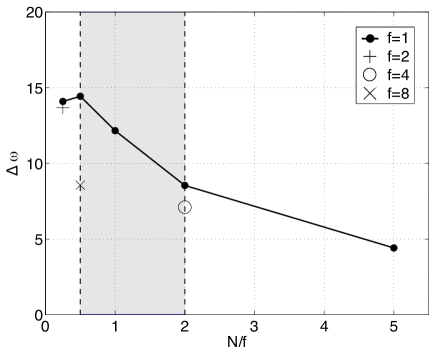
Figure 12: Measured dispersion of the energy around the theoretical dispersion relation of inertia-gravity waves, as a function of $N/f$ for several $256^{3}$ and $512^{3}$ simulations of rotating and stratified turbulence with varying Ro and Fr numbers. The range with no resonant interactions, $1/2\leq N/f\leq 2$, is indicated by the gray area. The dispersion for $f=1$ takes its maximum in this region. A few points for other values of $f$ are also shown.

In this section we present the spatio-temporal spectrum of several of the simulations discussed in Sec. IV. While extraction of waves and slow modes is often done using normal mode decompositions of the frozen in time fields in Fourier space Métais et al. (1996); Herbert et al. (2014); Marino et al. (2015b), these approaches are based on linearized equations and thus can mix ageostrophic modes with balanced components of the flow. Better identification of balanced modes can be achieved using higher-order expansions of the equations Dritschel and McKiver (2015). However, a precise separation of waves, mean winds, and eddies requiere information resolved in space and in time. In di Leoni et al. (2015) we introduced the spatio-temporal spectrum as a way to do this decomposition, and showed multiple applications including purely rotating di Leoni et al. (2014) and purely stratified flows di Leoni and Mininni (2015). The spatio-temporal spectrum was also used in recent laboratory experiments of rotating turbulence to study inertial waves Yarom and Sharon (2014); Campagne et al. (2015). The main objective of this section is to consider the rotating and stratified case, in particular in the range $1/2\leq N/f\leq 2$, and to use the spatio-temporal spectrum to quantify the relevance of wave modes and of slow modes. As discussed in Secs. III and IV, several effects in this range are believed to be associated with a dominance of slow modes and a relatively less importance of wave modes. The spatio-temporal spectrum will allow us to explicitly verify this is the case. However, as computation of the spatio-temporal spectrum requires very high temporal cadence, we will be able to do this analysis only in the simulations with $512^{3}$ grid points.

Computation of the spatio-temporal spectrum is performed by storing the Fourier coefficients of the fields ${\bf u}_{\bf k}(t)$ and $\theta_{\bf k}(t)$ with high temporal cadence (at least twice the period of the fastest waves). For each Fourier mode ${\bf k}$, the Fourier transform in time of these quantities results in $\hat{\bf u}({\bf k},\omega)$ and $\hat{\theta}({\bf k},\omega)$, which measure the phase and amplitude of each $({\bf k},\omega)$-mode in a four-dimensional space. The spatio-temporal spectrum can then be computed, e.g., for the kinetic energy, as

$$E_{V}({\bf k},\omega)=\frac{1}{2}|\hat{\bf u}({\bf k},\omega)|^{2}.$$ (45)

This spectrum quantifies the power in each wave vector ${\bf k}$ and frequency $\omega$, where ${\bf k}$ and $\omega$ are independent. In practice, waves, eddies, and other flow features satisfy some known relation $\omega=\omega({\bf k})$, and thus accumulation of energy over certain regions in the four-dimensional spectral space can be used to quantify how much energy is associated with these features. As an example, inertia-gravity waves correspond to an accumulation of energy in $({\bf k},\omega)$-modes satisfying

$$\omega=\omega_{\textrm{I-G}}({\bf k}),$$ (46)

where $\omega_{\textrm{I-G}}$ is the dispersion relation given in Eq. (16). From Eq. (18), advection of small-scale eddies by the large-scale velocity $U$ (i.e., sweeping) corresponds to the accumulation of energy in $({\bf k},\omega)$-modes satisfying

$$\omega\lesssim kU=\omega_{s}({\bf k}),$$ (47)

as at each ${\bf k}$ all eddies larger than the eddy size $\sim 1/k$ contribute to the Eulerian random sweeping. Doppler shift by a mean wind ${\bf W}$ appears as a shift of these relations by ${\bf W}\cdot{\bf k}$ di Leoni and Mininni (2015). A more detailed description of detection of energetic features in a flow using the spatio-temporal spectrum can be found in di Leoni et al. (2015).

Detection of waves in the four-dimensional spatio-temporal spectrum can be also simplified with some knowledge of what components of the fields are affected by the waves, depending on their polarization. For systems with $N/f\ll 1$, rotation is dominant and inertia-gravity waves reduce to inertial waves. Thus, in this case we can look at the spectrum of $u_{x}$ as for inertial waves the perturbation takes place in the plane perpendicular to $\Omega$. In contrast, for strongly stratified systems with $N/f\gg 1$ we should consider $u_{z}$ as this is the component of the velocity that is coupled to the temperature fluctuations in internal gravity waves. Thus, we consider the power spectrum of both components to allow identification of the waves as $N/f$ is varied.

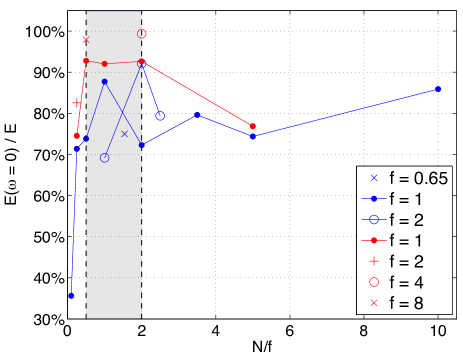
Figure 13: (Color online) Ratio of energy in modes with zero frequency to the total energy as a function of $N/f$ for several $256^{3}$ and $512^{3}$ simulations of rotating and stratified turbulence with varying Ro and Fr numbers. The range with no resonant interactions, $1/2\leq N/f\leq 2$, is indicated by the gray area. Note that the ratio takes the largest values in this region.

The spatio-temporal spectrum was computed for all $512^{3}$ simulations. Figures 10 and 11 show an illustration of these spectra for the runs with $N/f=1/4$ and with $N/f=1/2$ (this latter run in the range $1/2\leq N/f\leq 2$). These correspond respectively to runs 5 and 7 in Table 1. As the spectrum is four-dimensional, for $u_{x}$ we show slices for fixed values of $k_{x}$ and $k_{y}$, and show the spectrum as a function of $k_{z}$ and $\omega$, while for $u_{z}$ we show slices for fixed values of $k_{y}$ and $k_{z}$, and show the spectrum as a function of $k_{x}$ and $\omega$. The figures also indicate as a reference the theoretical dispersion relation of inertia-gravity waves, and the sweeping relation. The range of wave numbers shown in the figures correspond in all cases to wave numbers that should be dominated by waves, as in both simulations at least $k_{\textrm{Oz}}$ or $k_{\Omega}$ is larger than the maximum wave number considered. In run 5 (Fig. 10) $k_{\textrm{Oz}}\approx 5$ and $k_{\Omega}\approx 40$, thus rotation and stratification effects coexist for the smallest wave numbers, while for wave numbers in the range $5\lesssim k\lesssim 40$ rotation should be more relevant. In run 7 (Fig. 11) $k_{\textrm{Oz}}\approx 95$ and $k_{\Omega}\approx 270$ and inertia-gravity waves can be expected to be dominant at all wave numbers.

As a rule, excitation of modes lying over the theoretical dispersion relation can be observed for wave numbers such that the frequency of the waves is larger than the frequency of sweeping (i.e., for modes for which the waves are faster than the sweeping). This is to be expected as in wave turbulence, the fastest time scale controls the decorrelation of the modes di Leoni et al. (2014). But more interestingly, the dispersion of the energy around the dispersion relation of the waves varies with $N/f$. While the simulation with $N/f=1/4$ shows (for small wave numbers) a sharp concentration of energy around the relation $\omega_{\textrm{I-G}}({\bf k})$ (i.e., the theoretical dispersion relation of inertia-gravity waves), for $N/f=1/2$ the dispersion of the energy around this dispersion relation is much larger, and in some of the figures energy is concentrated in modes that do not correspond to wave excitations. Leaving aside the excitation of these modes associated with turbulence, the broadening of the energy near the dispersion relation in Fig. 11 can have multiple origins. As already discussed, sweeping results in broadening but it becomes dominant for wave numbers such that $\omega_{s}(k)>\omega_{\textrm{I-G}}({\bf k})$. Near-resonant and non-resonant wave interactions, which are expected to become relevant for $1/2\leq N/f\leq 2$, also result in broadening of the spectral peaks. Finally, eddy damping and turbulent fluctuations generate spectral broadening. Indeed, in this latter case weak turbulence theories and two point closures indicate that the broadening $\Delta\omega(k)$ is proportional to the inverse of the non-linear coupling time Sagaut and Cambon (2008); Nazarenko (2011); Miquel and Mordant (2011). For strong turbulence this is the eddy turnover time $\tau_{nl}$ given by Eq. (17). For an energy spectrum $E(k)$ between $\sim k^{-3}$ and $\sim k^{-2}$, this results in $\Delta\omega(k)$ being independent of the wave number or growing slowly as $k^{1/2}$.

A detailed analysis of the spatio-temporal spectra for all simulations is summarized in Figs. 12 and 13. Figure 12 shows the net dispersion of the energy around the theoretical wave dispersion relation as a function of $N/f$ for all $512^{3}$ runs. The net dispersion, e.g., for the power spectrum of the $x$ component of the velocity, is computed as

$$\Delta\omega=\frac{\sum_{{\bf k},\omega}|\omega({\bf k})-\omega_{\textrm{I-G}}({\bf k})|^{2}|u_{x}({\bf k},\omega)|^{2}}{\sum_{{\bf k},\omega}|u_{x}({\bf k},\omega)|^{2}},$$ (48)

and it corresponds to the the mean square differences between $\omega_{\textrm{I-G}}({\bf k})$ and the actual data, weighted by the spectral amplitude squared. As expected from the theoretical arguments, the maximum dispersion takes place in the range $1/2\leq N/f\leq 2$, for which resonant interactions vanish and either strong turbulence or near-resonant or non-resonant interactions prevail, also confirming the arguments in the previous sections. A few points for simulations with different values of $f$ are shown, which (for fixed $N/f$) show a smaller dispersion as $f$ is increased , to be expected as dispersion should decrease (i.e., more energy should be in the wave modes) as the strength of rotation and stratification increases.

From this data we can also compute the amount of energy in slow modes, that is to say, in modes with zero frequency. This is shown in Fig. 13, normalized by the total energy, for all simulations. In the figure there is a growth in this ratio in the region of non-resonant triads. Increasing the value of $f$ (and thus decreasing the Froude number) seems to increase the ratio, thus augmenting the amount of energy in modes with zero frequency. These results are consistent with those reported in Waite and Bartello (2006), where Waite and Bartello observed, for $\textrm{Ro}\approx 10^{-1}$, a growth in vortical energy as Ro decreases with fixed $N$. With three different values of $N$ (4, 8 and 16), they also concluded that the ratio of vortical energy to total energy is independent of the Rossby number. Our data, however, shows a dependence on the value of Ro, with smaller Ro resulting in more energy in the slow modes. The results are also consistent with recent studies of freely decaying stratified turbulence with varying Prandtl ratio Dritschel and McKiver (2015), where it was found that balance prevails in the flows for $N/f\gtrsim 1$. Finally, the trend of increasing energy in slow modes with decreasing Rossby is compatible with observations of inverse cascades in laboratory experiments of rotating flows Campagne et al. (2014) and with numerical studies in the low Rossby number limit Alexakis (2015), while they seem to be incompatible with the expected decoupling of the slow modes in that limit Greenspan (1968); Cambon et al. (2004). This can be the result of finite-domain effects in the numerical simulations Cambon et al. (2004), or the result of higher-order corrections to the linear stability theory Alexakis (2015).

VI Conclusions

Inverse cascades play a central role in geophysical turbulence, providing a mechanism for the formation of large-scale structures and for the self-organization of disorganized flows. Since Kraichnan contribution, extensions of his ideas to quasi-geostrophic turbulence, rotating flows, and rotating and stratified flows have been developed as a way to better describe atmospheric and oceanic processes. In this context, here we reviewed several recent studies of inverse cascades in rotating and stratified turbulence.

Special emphasis was put on reviewing the dependence of scaling laws, anisotropy, and the strength of the inverse cascade on the inverse Prandtl ratio $N/f$ of the Coriolis frequency to the Brunt-Väisäla frequency. We showed that while the anisotropy and the ratio of perpendicular to parallel length scales varies linearly with $N/f$ (in particular in the range $1/2\leq N/f\leq 2$), the strength of the inverse cascade depends non-monotonically on this parameter, with the inverse cascade being faster in this range, and then decreasing monotonically as $N/f$ is increased.

This behavior can be explained by considering that in the range $1/2\leq N/f\leq 2$ no resonant triadic interactions between waves are available. Thus, quasi-geostrophic motions are expected to dominate the dynamics. Previous studies (see, e.g., Bartello (1995); Métais et al. (1996); Reinhaud et al. (2003); Waite and Bartello (2004, 2006); Kurien et al. (2008)) have confirmed this by indirect measures, such as, e.g., normal mode decomposition of frozen in time fields to separate wave modes from slow modes, or higher-order expansions of the equations to separate the flow in terms of balanced and imbalanced components Dritschel and McKiver (2015). Here we presented a new analysis based on fully resolved spatio-temporal information, using the spectrum as a function of the wave vector and frequency to measure how much energy is excited in modes compatible with the dispersion relation of the waves, and in the rest of the modes.

The simulations confirmed the linear scaling of the ratio of the perpendicular to parallel velocity with $N/f$ in the range $1/2\leq N/f\leq 2$, and also showed that accumulation of energy near wave modes in the spatio temporal spectrum is minimal in this range, while energy in slow modes becomes larger. This is in good agreement with previous results using different methods for the analysis, and sheds new light on reasons for the fast inverse cascade of 3D rotating and stratified turbulent flows reported previously in Marino et al. (2013).

Fifty years after the paper by Kraichnan on inverse cascades in two dimensional flows Kraichnan (1967), there remains much to be done to understand turbulent phenomena in the real world. The study of inverse cascades in more realistic scenarios has just started, and the previous works reviewed here, as well as the new results, consider small Reynolds numbers, periodic boundary conditions, or infinite domains which put them far away from real applications. As in the paper written by Kraichnan and Montgomery Kraichnan and Montgomery (1980), it is however our hope that some of the results of these studies can be translated to atmospheric and oceanographic problems. Recent studies considering observations in the atmosphere and the ocean (see, e.g., Scott and Wang (2005); Sukoriansky et al. (2007); Schlösser and Eden (2007) and references therein) seem to indicate that indeed the gap between idealized simulations and real measurements of the inverse cascade can be bridged.