Dark stars: gravitational and electromagnetic observables

Abstract

Theoretical models of self-interacting dark matter represent a promising answer to a series of open problems within the so-called collisionless cold dark matter (CCDM) paradigm. In case of asymmetric dark matter, self-interactions might facilitate gravitational collapse and potentially lead to formation of compact objects predominantly made of dark matter. Considering both fermionic and bosonic equations of state, we construct the equilibrium structure of rotating dark stars, focusing on their bulk properties, and comparing them with baryonic neutron stars. We also show that these dark objects admit the $I$-Love-$Q$ universal relations, which link their moments of inertia, tidal deformabilities, and quadrupole moments. Finally, we prove that stars built with a dark matter equation of state are not compact enough to mimic black holes in general relativity, thus making them distinguishable in potential events of gravitational interferometers.

I Introduction

It is quite probable that if dark matter (DM) exists in the form of particles, it might experience non-negligible self-interactions. This is highly motivated both theoretically and observationally. From a theoretical point of view, if the dark sector is embedded in a unification scheme in a theory beyond the Standard Model, it is hard to imagine DM particles that do not interact among themselves via some gauge bosons. In addition, DM self-interactions might be a desirable feature due to the fact that the CCDM paradigm seems to be currently at odds with observations. There are three main challenges that CCDM faces today. The first one is related to the flatness of the DM density profile at the core of dwarf galaxies Moore (1994); Flores and Primack (1994). The latter are dominated by DM and, although numerical simulations of CCDM Navarro et al. (1997) predict a cuspy profile for the DM density at the core of these galaxies, measurements of the rotation curves suggest that the density profile is flat. A second issue is that numerical simulations of CCDM also predict a larger number of satellite galaxies in the Milky Way than what has been observed so far Klypin et al. (1999); Moore et al. (1999); Kauffmann et al. (1993). Finally a third serious problem for CCDM is the “too big to fail”  Boylan-Kolchin et al. (2011), i.e. CCDM numerical simulations predict massive dwarf galaxies that are too big to not form visible and observable stars. These discrepancies between numerical simulations of CCDM and observations could be alleviated by taking into account DM-baryon interactions Oh et al. (2011); Brook et al. (2012); Pontzen and Governato (2012); Governato et al. (2012). In addition, the satellite discrepancy could be attributed to Milky Way being a statistical fluctuation Liu et al. (2011); Tollerud et al. (2011); Strigari and Wechsler (2012), thus deviating from what numerical simulations predict. Apart from these explanations, another possible solution is the existence of substantial DM self-interactions, which can solve all three aforementioned problems Vogelsberger et al. (2012); Rocha et al. (2013); Zavala et al. (2013); Peter et al. (2013). It is not hard for example to see that DM self-interactions would lead to increased rates of self-scattering in high DM density regions, thus flattening out dense dwarf galaxy cores.

In this picture, DM self-interactions have been thoroughly studied in the literature in different contexts Spergel and Steinhardt (2000); Wandelt et al. (2000); Faraggi and Pospelov (2002); Mohapatra et al. (2002); Kusenko and Steinhardt (2001); Loeb and Weiner (2011); Kouvaris (2012); Rocha et al. (2013); Peter et al. (2013); Vogelsberger and Zavala (2013); Zavala et al. (2013); Tulin et al. (2013); Kaplinghat et al. (2014a, b); Cline et al. (2014a, b); Petraki et al. (2014); Buckley et al. (2014); Boddy et al. (2014); Schutz and Slatyer (2015). Although depending on the type of DM self-interactions, the general consensus is that DM interactions falling within the range $0.1~{}\text{cm}^{2}/\text{g}<\sigma_{XX}/m_{X}<10~{}\text{cm}^{2}/\text{g}$ ($\sigma_{XX}$ and $m_{\textnormal{X}}$ being the DM self-interaction cross section and DM particle mass respectively) are sufficient to resolve the CCDM problems. If DM is made of one species, DM self-interactions cannot be arbitrarily strong because in this case they could destroy the ellipticity of spiral galaxies Feng et al. (2009, 2010), dissociate the bullet cluster Markevitch et al. (2004) or destroy old neutron stars (NSs) by accelerating the collapse of captured DM at the core of the stars leading to formation of black holes that could eat up the star (thus imposing constraints due to observation of old NSs) Kouvaris et al. (2015).

Apart from the associated problems of CCDM, there is another orthogonal scenario where DM self-interactions might be needed. The supermassive black hole at the center of the Milky Way seems to be too big to have grown within the lifetime of the galaxy from collapsed baryonic stars. One possible solution is to envision a strongly self-interacting subdominant component of DM that collapses via a gravothermal process, providing the seeds for the black hole to grow to today’s mass within the lifetime of the Milky Way Pollack et al. (2015).

As a desirable feature of DM, self-interactions may assist DM clumping together and forming compact objects, if they are dissipative or they speed up gravothermal evolution Balberg et al. (2002). There could be two different possibilities here: i) DM with substantial amount of annihilations and ii) DM with negligible amount of annihilations. The Weakly Interacting Massive Particle (WIMP) paradigm belongs to the first category. In this case, the DM relic density in the Universe is determined by the DM annihilations. DM is in thermal equilibrium with the primordial plasma until the rate of DM annihilations becomes smaller than the expansion of the Universe. In this WIMP paradigm, particle and antiparticle populations of DM come with equal numbers. Gravitational collapse of such type of DM could create dark stars that oppose further gravitational collapse by radiation pressure Spolyar et al. (2008); Freese et al. (2009, 2008). However, these types of stars cannot exist anymore, as DM annihilations would have already lead to the depletion of the DM population and therefore to the extinction of these dark stars long time ago.

On the contrary, asymmetric DM can lead to the formation of compact star-like objects that can be stable today. The asymmetric DM scenario is a well-motivated alternative to the WIMP paradigm Nussinov (1985); Barr et al. (1990); Gudnason et al. (2006); Foadi et al. (2009); Dietrich and Sannino (2007); Sannino (2009); Ryttov and Sannino (2008); Sannino and Zwicky (2009); Kaplan et al. (2009); Frandsen and Sannino (2010); March-Russell and McCullough (2012); Frandsen et al. (2011); Gao et al. (2013); Arina and Sahu (2012); Buckley and Profumo (2012); Lewis et al. (2012); Davoudiasl et al. (2011); Graesser et al. (2011); Bell et al. (2011); Cheung and Zurek (2011). In this case, there is a conserved quantum number, as, e.g., the baryon number. A mechanism similar to the one responsible for the baryon asymmetry in the Universe could also create a particle-antiparticle asymmetry in the DM sector. DM annihilations deplete the species with the smaller population, leaving at the end only the species in excess, to account for the DM relic density. One can easily see that, e.g., a DM particle of mass $\sim 5$ GeV could account for the DM abundance, provided that a common asymmetry mechanism that creates simultaneously a baryon and a DM unit is in place. Obviously, in such an asymmetric DM scenario, there is no substantial amount of annihilations today due to lack of DM antiparticles. Therefore, provided that DM self-interactions can facilitate the collapse, asymmetric DM can form compact objects that can be stable, thus possibly detectable today via, e.g., gravitational wave (GW) emission in binary systems.

The possibility of asymmetric DM forming compact-like objects has been studied both in the case of fermionic Narain et al. (2006); Kouvaris and Nielsen (2015) as well as bosonic Eby et al. (2016a) DM. In both of these papers, the mass–radius relations, density profiles, and maximum “Chandrasekhar” mass limits were established for a wide range of DM particle masses and DM self-coupling, for both attractive and repulsive interactions. Bosonic DM forming compact objects has also been studied in other than asymmetric DM contexts, i.e., in the case DM is ultra light, e.g., axions Kolb and Tkachev (1993, 1994); Chavanis (2011); Chavanis and Delfini (2011); Eby et al. (2015); Brito et al. (2016a); Eby et al. (2016b, c); Cotner (2016); Davidson and Schwetz (2016); Chavanis (2016); Levkov et al. (2017); Hui et al. (2017); Bai et al. (2016); Eby et al. (2017) or other theoretically motivated bosonic candidates Soni and Zhang (2016)

These proposed dark stars, if in binary systems, can produce GW signals that could potentially distinguish them from corresponding signals of black hole binaries, as it was suggested in Giudice et al. (2016); Cardoso et al. (2017). Other probes of bosonic DM stars via GWs have been proposed in Dev et al. (2016). We remark that objects inconsistent with either black holes or NSs may suggest the existence of new particle physics. Therefore, compact binary mergers could become a search strategy for beyond-standard-model physics which is completely orthogonal to the LHC and (in-)direct DM searches. Interesting scenario of compact objects made of asymmetric DM with a substantial baryonic component has also been studied Leung et al. (2011, 2013); Tolos and Schaffner-Bielich (2015); Mukhopadhyay and Schaffner-Bielich (2016).

One should mention that there are several scenarios of how these dark stars can form in the first place. Gravothermal collapse is one option Lynden-Bell and Wood (1968). In this case, DM self-interactions facilitate the eviction of DM particles that acquire excessive energy from DM-DM collisions, thus leading to a lower energy DM cloud that shrinks gradually forming a dark star. Another possibility is by DM accretion in supermassive stars. Once the star collapses, DM is not necessarily carried by the supernova shock wave, leaving a highly compact DM population at the core Kouvaris and Tinyakov (2010). Moreover, if DM interactions are dissipative, DM can clump via direct cooling Fan et al. (2013).

It is crucial to determine the most important features which characterize the bulk properties of dark compact objects, and form a set of suitable observables to be potentially constrained by gravitational and electromagnetic surveys. In this paper, we investigate the structure of slowly-rotating and tidally-deformed stars, modeled with a DM equation of state (EoS), based on fermionic and bosonic DM particles. As far as rotation is concerned, we follow the approach developed in Hartle (1967); Hartle and Thorne (1968), in which spin corrections are described as a small perturbation of a static, spherically symmetric spacetime. At the background level, the star structure is determined by solving the usual Tolman-Oppenheimer-Volkoff equations (TOV). Rotational terms are included up to second order in the angular momentum $J$, which allow to compute the moment of inertia $I$ and the quadrupole moment $Q$ of the star. Similarly, we model tidal effects through the relativistic perturbative formalism described in Hinderer (2008). At leading order, this approach leads to the Love number $k_{2}$, or, equivalently, the tidal deformability $\lambda=2/3k_{2}R^{5}$, which encodes all the properties of the star’s quadrupolar deformations. We refer the reader to the references cited above for a detailed description of the equations needed to compute these quantities.

The plan of the paper is the following: In Sec. II we describe the main properties of the two classes of the dark EoS considered. In Secs. III and IV we analyze the bulk properties of the stellar models, such as masses and radii, which can be potentially constrained through electromagnetic and GW observations. An explicit example of such constraints is discussed in Sec. IV.1. In Sec. V we investigate universal relations for dark stars. Finally, in Sec. VI we summarize our results.

Throughout the paper (with the exception of Sec. II and the Appendix) we use geometrized units, in which $G=c=1$.

II The dark matter equation of state

In this section we describe the most important features of the dark EoS used in this paper to model fermion and boson stars. Moreover, in our analysis we will also consider two standard EoS, apr Akmal et al. (1998) and ms1 Muller and Serot (1995), which represent two extreme examples of soft and stiff nuclear matter, and will allow to make a direct comparison between the macroscopic features of baryonic and dark objects.

II.1 Fermion star

We consider a fermionic particle interacting via a repulsive Yukawa potential (e.g., due to a massive dark photon):

$$V=\frac{\alpha_{\textnormal{X}}}{r}\exp\left(-\frac{\hbar m_{\phi}r}{c}\right),$$ (1)

where $\alpha_{X}$ is the dark fine structure constant and $m_{\phi}$ is the mass of the mediator. The mass of the DM fermion is denoted as $m_{\textnormal{X}}$. Models that interact through a Yukawa potential are useful in the context of self-interacting DM, because the scattering cross section is suppressed at large relative velocities Tulin et al. (2013). As a result, the success of collisionless cold DM is left untouched at super-glactic scales, while sub-galactic structure is flattened. In the context of self-interacting DM, both attractive and repulsive interactions flatten structures. However, attractive interactions in a compact object will soften the EoS. Since we are interested in dense objects, we only consider repulsive interactions.

Pressure in fermion stars has two contributions: one from Fermi-repulsion and one due to the Yukawa-interactions. We calculate the energy density and pressure due to Yukawa interactions in the mean field approximation; in this case the EoS is given by two implicitly related equations (see Kouvaris and Nielsen (2015) for further details):

$$\rho =\frac{m_{\textnormal{X}}^{4}c^{3}}{\hbar^{3}}\left[\xi(x)+\frac{2}{9\pi^{3}}\frac{\alpha_{\textnormal{X}}}{\hbar c}\frac{m_{\textnormal{X}}^{2}}{m_{\phi}^{2}}x^{6}\right],$$ (2a)

$$P =\frac{m_{\textnormal{X}}^{4}c^{5}}{\hbar^{3}}\left[\chi(x)+\frac{2}{9\pi^{3}}\frac{\alpha_{\textnormal{X}}}{\hbar c}\frac{m_{\textnormal{X}}^{2}}{m_{\phi}^{2}}x^{6}\right],$$ (2b)

where $x\equiv p_{\text{F}}/(m_{\textnormal{X}}c)$ is a dimensionless quantity that measures the Fermi-momentum compared to the DM mass (note that the density is defined such that $\rho c^{2}$ is the total energy density). The functions $\xi$ and $\chi$ are the contributions from Fermi-repulsion Shapiro and Teukolsky (1983), given by

$$\xi(x) =\frac{1}{8\pi^{2}}\left[x\sqrt{1+x^{2}}(2x^{2}+1)-\ln\left(x+\sqrt{1+x^{2}}\right)\right],$$

$$\chi(x) =\frac{1}{8\pi^{2}}\left[x\sqrt{1+x^{2}}(2x^{2}/3-1)+\ln\left(x+\sqrt{1+x^{2}}\right)\right].$$

Both pressure and density are smooth monotonic functions of the parameters $x$. At low density the EoS becomes an approximate polytrope $P=K\rho^{\gamma}$ with index $\gamma\simeq 5/3$, whereas at large density the index changes to $\gamma\simeq 1$. At large density the proportionality constant is $K=c^{2}/3$ or $K=c^{2}$, depending on whether the Fermi-repulsion or the Yukawa-interactions dominates, respectively.

II.2 Boson star

Boson stars are naturally much smaller than their fermionic counterparts, because they lack Fermi-pressure to balance their self-gravity Kaup (1968); Ruffini and Bonazzola (1969). In the absence of self-interactions, bosons stars are stabilized by a quantum mechanical pressure due to the uncertainty principle. Unless the bosons are extraordinarily light, this pressure is inherently tiny and can only balance small lumps of matter. If the field self-interacts, the boson star would naturally be similar to a fermion star in size Colpi et al. (1986).

A wide variety of boson stars have been investigated in the literature (see Liebling and Palenzuela (2012) for a comprehensive review). The most studied examples include a complex scalar field with a $U(1)$ symmetry and an associated Noether charge. Other solutions include: real scalar field oscillatons Seidel and Suen (1991), Proca stars Brito et al. (2016b), and axion stars Sikivie and Yang (2009), to name a few. In this work, we consider a complex scalar field coupled to gravity with the action

$$S_{\text{BS}}=\int d^{4}x\sqrt{-g}\left(\frac{c^{4}R}{16\pi G}-|\partial_{\mu}\phi|^{2}-\frac{m_{\textnormal{X}}^{2}c^{2}}{\hbar^{2}}|\phi|^{2}-\frac{1}{2}\frac{\beta}{\hbar c}|\phi|^{4}\right),$$ (3)

where $m_{\textnormal{X}}$ is the boson mass and $\beta$ is a dimensionless coupling constant. The energy-momentum tensor is not automatically isotropic for a boson star. As such, the TOV formalism does not always apply. However, if we choose a spherically symmetric ansatz for the metric and the field [$\phi=\varphi(r)e^{i\omega t}$], the energy-momentum tensor becomes approximately isotropic. The EoS for this boson star model was first derived in Colpi et al. (1986) and it is given by

$$P=\frac{c^{5}}{9\hbar^{3}}\frac{m_{\textnormal{X}}^{4}}{\beta}\left(\sqrt{1+\frac{3\hbar^{3}}{c^{3}}\frac{\beta\rho}{m_{\textnormal{X}}^{4}}}-1\right)^{2}.$$ (4)

This EoS behaves as a $\gamma\simeq 2$ polytrope at low density, and smoothly softens to $\gamma\simeq 1$ at high density.

III Mass - radius profiles

Masses and radii are the macroscopic quantities which immediately characterize astrophysical compact objects, and they represent the primary target of both gravitational and electromagnetic surveys. X-ray and radio observations of astrophysical binaries are expected to provide precise measurements of the mass components, as they develop multiple relativistic effects which can be used to independently constrain the stellar structure Will (2014); Lattimer and Prakash (2007). However, an accurate estimate of the radius still represents a challenging task, mostly relied upon the observation of signals coming from the interaction of the star with its surrounding environment, which strongly depends on the assumption employed to model the process. Coalescences of binary NSs are also among the most powerful sources of GWs for ground-based interferometers, like LIGO Aasi et al. (2015) and Virgo Acernese et al. (2015), as the large number of cycles before the merger will allow to extract the mass of the objects with good accuracy Sathyaprakash and Schutz (2009). Moreover, unlike the EM bandwidth, GW observatories have access to another quantity, the tidal deformability Flanagan and Hinderer (2008); Hinderer (2008), which offers complementary information about the stellar radius (see Sec. IV).

These considerations point out that it is crucial to understand how the values of $M$ and $R$ change according to the extra parameters which specify the DM sector, and to which extent they differ from ordinary NSs. The first section of our analysis will be therefore devoted to investigate these features.

III.1 Fermion stars

The fermion stars described in this paper are fully specified by three parameters: the coupling constant $\alpha_{\textnormal{X}}$, the dark particle mass $m_{\textnormal{X}}$, and the mediator mass $m_{\phi}$. Hereafter, we will fix $\alpha_{\textnormal{X}}/\hbar c\equiv\alpha=10^{-3}$, varying the other two coefficients $m_{\phi}=(8,10,12)$MeV and $m_{X}=(1,2)$GeV. These values lead to mass–radius profiles comparable with those computed for apr and ms1, and therefore will allow for a direct and more clear comparison with NSs. All our models, identified by the label $\phi\texttt{m}_{\phi}\_\texttt{X}\texttt{m}_{\texttt{X}}$, are presented in Fig. 1. Each point of the plot is obtained, for a chosen EoS, by varying the star’s central pressure.

The left panel of the plot shows how the dark sector parameters affect the stellar configurations. We note first that, for a fixed radius, larger values of $m_{\textnormal{X}}$ rapidly decrease the mass, therefore leading to less compact objects. This is more evident from the center panel in which we draw the compactness ${\cal C}=M/R$ for all of our models. The mediator mass also provides large changes, still in the same direction as $m_{\textnormal{X}}$, as less compact stars are obtained passing from $m_{\phi}=8$MeV to $m_{\phi}=12$MeV. It is interesting to note that the two baryonic EoS considered are characterized by steeper slopes, which lead to larger mass/radius variations. Both left and center plots also show that overlapping regions do exist between fermion stars and baryonic matter profiles which yield the same configurations. This is particularly relevant from the experimental point of view, as mass and radius measurements lead to degeneracies which may prevent a clear identification of the nature of the compact object.

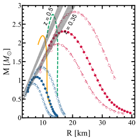
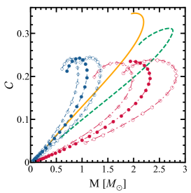
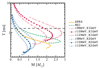
Figure 1: (Left) Mass-radius profiles for fermion stars with fixed $\alpha=10^{-3}$, dark particle mass $m_{X}=(1,2)$GeV, and mediator mass $m_{\phi}=(8,10,12)$MeV. The standard EoS apr and ms1 are represented by the yellow solid and the dashed green curves respectively. The shaded regions correspond to contour regions of constant surface redshift $z=0.35$ and $z=0.5$ with 10% of accuracy. (Center) Compactness ${\cal C}=M/R$ as a function of the stellar mass, for the models considered in the left panel. (Right) Minimum period, according to the Kepler frequency limit, $T=2\pi/\Omega_{\textnormal{K}}$. The dashed horizontal line represents the fastest known pulsar with $f=716$ Hz.

Mass-radius profiles are extremely useful, since they can exploit astrophysical observations to constrain the space of nuclear EoS. As an example, in the left plot of Fig. 1 we show two shaded regions corresponding to constant surface redshift

$$z=\left(1-\frac{2M}{R}\right)^{-1/2}-1\ ,$$ (5)

with two reference values, namely $z=0.35$ and $z=0.5$. The first one matches the data obtained for EXO 0748-676, a NS showing repeated X-ray bursts Cottam et al. (2002). The width of the bands represents a 10% of accuracy in the measurements. It is clear that, in the first case ($z=0.35$), the observed value is already inconsistent with all the stable branches of the models considered in this section. However, a potential observation of a surface redshift $z=0.5$ would set a tighter bound, ruling out the possibility that the source is a fermion star with one of the EoS we have used here. Using multiple observables, like the Eddington flux and the ratio between the thermal flux and the color temperature, would further reduce the parameter space of allowed configurations

The center panel of Fig. 1 shows another interesting property of fermion stars. The EoS considered cover large changes in the mass–radius space, but the corresponding compactness never exceeds a threshold ${\cal C}\approx 0.22$, contrary to apr and ms1, which can achieve values higher than $0.3$. Although significantly different from white dwarf and main-sequence stars (with ${\cal C}\lesssim 10^{-6}$), this indicates that fermion stars cannot act as black hole mimickers, i.e., compact objects with a compactness approaching the limit value ${\cal C}\rightarrow 0.5$ Cardoso et al. (2017); Völkel and Kokkotas (2017).

As a final remark, for each model it is useful to investigate the maximum rotation rate allowed by the stellar structure. This quantity is of particular interest for astrophysical observations, as spinning frequencies of isolated and binary NSs are measured with exquisite precision and they can be used to constrain the underlying EoS Lattimer and Prakash (2007). The right panel of Fig. 1 shows the minimum rotational period for fermion stars, derived from the Keplerian limit $T=2\pi/\Omega_{\textnormal{K}}$, where $\Omega_{\textnormal{K}}\approx\sqrt{M/R^{3}}$ (mass-shedding limit). Although this is a Newtonian approximation, it gives a good estimate of the order of magnitude of this quantity, and provides an absolute upper limit on the spin. As a benchmark, we also draw (horizontal black line) the value corresponding to the maximum frequency observed for a spinning NS, $f=716$ Hz, i.e., $T\approx 1.4$ ms Hessels et al. (2006). This constraint alone cannot rule out any theoretical model that we have used to describe both dark stars and regular NSs. Assuming a future dark star observation, a bound potentially able to exclude configurations with $m_{\textnormal{X}}\lesssim 1$GeV would require a much faster rotating object, with $f\approx 1800$Hz or, equivalently, $T\approx 0.55$ ms.

III.2 Boson stars

The mass–radius profiles for boson stars are shown in the left panel of Fig. 2. We consider three values of the coupling parameter $\beta=(0.5,1,1.5)\pi$ and two values of the boson mass $m_{\textnormal{X}}=(300,400)$MeV. Like the fermion case, these configurations are chosen to provide the stellar models closest to the standard NSs built with apr and ms1. We label the boson EoS as $\beta\_\texttt{X}\texttt{m}_{\texttt{X}}$.

We first note that, for a given mass, stronger couplings stiffen the EoS, leading to larger radii and, therefore, to less compact objects. At the same time, $\beta$ modifies the maximum mass of each model, shifting the value to the top end of the parameter space. The same trend, although with a major impact, occurs if we consider lighter dark particles.

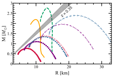
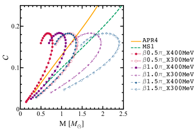
Figure 2: Same as Fig. 1, but for boson stars with different values of the coupling constant $\beta=(0.5,1,1.5)\pi$ and boson mass $m_{\textnormal{X}}=(300,400)$MeV.

Even for boson stars, the slope of the curves is smoother than that obtained for standard nuclear matter. This produces more pronounced changes in the radius distribution, as the central pressure of the star varies. The right panel of Fig. 2 also shows the stellar compactness $M/R$. For all the considered models, we observe a maximum value ${\cal C}\approx 0.16$, well below the edge of the curve related to apr and ms1 which, for a fixed radius, yield softer EoS and therefore larger masses. This also excludes the chance to interpret boson stars as astrophysical objects compact enough to mimic black holes. Remarkably, we find that this peoperty holds in general for any class of boson EoS, independently from the coupling parameter. A mathematical proof of this feature is outlined in the Appendix.

Electromagnetic observations of the stellar spin frequency are still too weak to considerably narrow the star parameter space, as the maximum value observed so far leaves the EoS essentially unbound. Larger values of $f\approx 1400$ Hz (or, equivalently, $T\approx 0.7$ ms) would be required to exclude the presence of a dark star. On the other hand, as seen in the previous section, precise measurements of the surface redshift represent a powerful tool to constrain the stellar structure. As an example, the value $z=0.35$, derived for EXO 0748-676, seems already to exclude the possibility that this object is built by one of the bosonic EoS considered.

IV Moments of inertia, tidal Love numbers and quadrupole moments

The moment of inertia represents another global feature of compact objects, potentially observable by electromagnetic surveys, which depends more on the compactness ${\cal C}$ rather than on the microphysical details of the EoS. The moment of inertia is found to be correlated through semi-analytical relations with different stellar parameters, scaling approximately as $R^{2}$. Therefore, any constraint on the stellar radius naturally provides a bound for $I$ Lattimer and Prakash (2001); Lattimer and Lim (2013). Moreover, this quantity affects different astrophysical processes, such as pulsar glitches, characterized by sudden increases of the stellar rotational frequency (of the order of $10^{-6}$). The relativistic spin-orbit coupling in compact binary systems also depends on the moment of inertia. In the near future, high precision pulsar timing could determine the periastron advance of such systems in order to provide an estimate of $I$ (and therefore of $R$) with an accuracy of $10\%$ Lattimer and Schutz (2005).

Motivated by these considerations, in this section we shall compare the values of the moment of inertia computed for DM and baryonic EoS. Our results are shown in Fig. 3. As expected, for fermion stars and a fixed stellar mass, $I$ increases for smaller values of $m_{\phi}$ and $m_{\textnormal{X}}$, with the latter leading to the largest variations, as it mainly affects the stellar compactness. For the boson case, the largest moment of inertia results from light particles, with $m_{\textnormal{X}}<300$ MeV, and stronger repulsive interactions $\beta\gtrsim\pi$. We also note that for fermion stars and a fixed mass $m_{\textnormal{X}}$, the spread within the configurations given by the mediator $\phi$, typically $\Delta I\gtrsim 10\%$, is much larger than the gap between apr and ms1, which cover a rather wide range of standard EoS currently known. This is particularly relevant for future space observations, as measurements of the spin-orbit effect (previously described) would provide errors smaller or equal to $\Delta I$, and therefore would be able to set (at least) an upper bound on $m_{\phi}$. Similar considerations also apply to the boson sector, if we consider the deviations produced by the coupling parameter $\beta$.

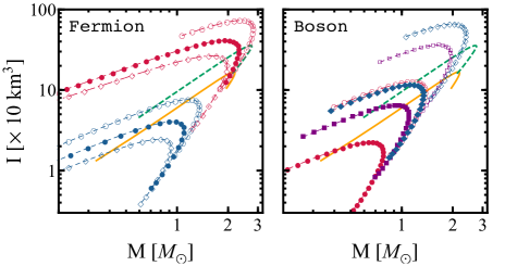
Figure 3: Moment of inertia for fermion (left) and boson (right) stars, for the various EoS considered in Figs. 1-2. The yellow solid and green dashed curve correspond to the apr and ms1 EoS, respectively.

Extracting information on the internal structure of compact objects is also a primary goal of current and future GW interferometers. The imprint of the EoS within the signals emitted during binary coalescences is mostly determined by adiabatic tidal interactions, characterized in terms of a set of coefficients, the Love numbers, which are computed assuming that tidal effects are produced by an external, time-independent gravitational field Hinderer (2008); Binnington and Poisson (2009); Damour and Nagar (2009). The dominant contribution $k_{2}$, associated to a quadrupolar deformation, is defined by the relation

$${\cal Q}_{ij}=\frac{2}{3}k_{2}R^{5}{\cal E}_{ij}=\lambda{\cal E}_{ij}\ ,$$ (6)

where ${\cal E}_{ij}$ is the external tidal tensor and ${\cal Q}_{ij}$ is the (tidally-deformed) star’s quadrupole tensor. The Love number $k_{2}$ or, equivalently, the tidal deformability $\lambda$, depends solely on the star’s EoS. The inclusion of the Love number into semi-analytical templates for GW searches, and its detectability by current and future detectors, have been deeply investigated in the literature Flanagan and Hinderer (2008); Damour and Nagar (2010); Maselli et al. (2013a); Damour et al. (2012); Hinderer et al. (2010); Bernuzzi et al. (2012); Read et al. (2013); Baiotti et al. (2010, 2011); Vines et al. (2011); Pannarale et al. (2011); Vines and Flanagan (2013); Lackey et al. (2012, 2014); Yagi and Yunes (2014). As an example, fully relativistic numerical simulations have shown that, for stiff EoS, the radius of a standard NS can be constrained within $\sim 10\%$ of accuracy by advanced detectors, with the measurability rapidly getting worse for softer matter, i.e., for stellar configurations with larger compactness Hotokezaka et al. (2016). More recently, the effect of dynamic tides has been taken into account, proving that they also provide a significant contribution to the GW emission Hinderer et al. (2016); Essick et al. (2016).

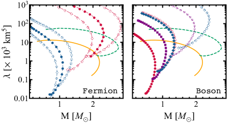
Figure 4: Same as Fig. 3 but for the tidal deformability $\lambda$.

To this end, it is crucial to analyze how $\lambda$ behaves for dark stars, as they may lead to large signatures, potentially detectable by GW interferometers, to be used together with measurements of $I$ and $Q$ for multi-messenger constraints. Figure 4 shows the tidal deformability as a function of the stellar mass, for fermion and boson stars. For the former, different values of $m_{\textnormal{X}}$ and $m_{\phi}$ yield large variations of $\lambda$ within the parameter space. Such differences are mainly related to the strong dependence of the tidal deformability on the stellar radius, $\lambda\propto k_{2}R^{5}$, which amplifies the discrepancies between the models. We also note that for boson stars a universal relation between $k_{2}$ and the compactness ${\cal C}=M/R$ exists, which is independent of the specific choice of $m_{X}$ and $\beta$.

It is worth to remark that these features, which ultimately reflects the stellar compactness, may be a crucial ingredient for future GW detections, as $\lambda$ is the actual parameter entering the waveform. In this regard, dark stars with a lighter mediator $\phi$ would experience large deformations, improving our ability to constrain the tidal Love number. On the other hand, EoS with $m_{\phi}\gg 1$GeV would provide smaller $\lambda$, leading to weaker effects within the signal and, hence, to looser bounds on the star’s structure.

Similar considerations hold as far as boson interactions are taken into account. For a chosen mass, both larger couplings and lighter particles lead to larger values of the Love number. The right panel of Fig. 4 shows indeed that for a canonical $1.4M_{\odot}$ star, even a very stiff EoS like ms1 would provide a tidal deformability more than two orders of magnitude smaller than those computed for $\beta\gtrsim\pi$ and $m_{\textnormal{X}}\lesssim 300$MeV. Such enhancement would strongly improve the measurability of $\lambda$ from GW signals.

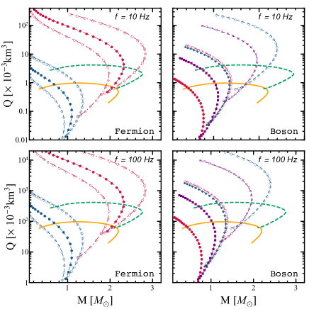
Figure 5: Quadrupole moments as functions of the stellar mass $M$ for two values of the rotational frequency $f=(10,100)$Hz. The data for fermion and boson stars are compared against the results derived for the standard EoS apr and ms1.

As a final remark, in Fig. 5 we show the spin-induced quadrupole moment for fermion and boson stars. Following Hartle and Thorne (1968); Hartle (1967), the spacetime describing a spinning compact object can be obtained perturbing a spherical non-rotating metric, as a power series of the dimensionless spin variable $\chi=J/M^{2}$, $J$ being the star’s intrinsic angular momentum. The quadrupole moment affects the perturbed metric at the second order in $\chi$. In our analysis we consider rotational frequencies $f=(10,100)$Hz, such that $\chi\ll 1$, i.e., requiring that spin effects represent a small perturbation of the static, spherically symmetric background. Looking at the figure we immediately note that, for a fixed mass, the values of $Q$ for dark and neutron stars yield large differences, which can be potentially tested both by GW and electromagnetic observations. Indeed, the quadrupole moment modifies the gravitational waveform produced by binary coalescences, leading to signatures detectable by terrestrial interferometers Krishnendu et al. (2017). Moreover, $Q$ is expected to affect the location of the innermost stable circular orbit, and therefore to influence the geodesic motion around the star Pappas (2012). The latter plays a crucial role in several astrophysical phenomena related to accretion processes, which produce characteristic signals (quasi-periodic oscillations), that have been proven to be a powerful diagnostic tool of the nature of gravity in the strong-field regime.

IV.1 Constraining the bulk properties: a practical example

Before further discussing the basic properties of boson and fermion stars, it is useful to provide an explicit example of how future observations will constrain the bulk properties described in the previous sections. For the sake of simplicity, we shall consider one particular quantity, the tidal deformability $\lambda$, which affects the GW signals emitted by binary systems. We consider indeed the coalescence of two non-spinning dark stars with masses $m_{1},m_{2}$ and the same EoS. The emitted sky-averaged waveform in the frequency domain

$$\tilde{h}(f)={\cal A}e^{i\psi(f)}\ ,$$ (7)

is specified by the overall amplitude ${\cal A}$ and the phase $\psi(f)$, which depends on the GW frequency $f$ and the physical parameters $\bm{\theta}=({\cal A},\ln{\cal M},\ln\nu,t_{c},\phi_{c},\Lambda)$, where ${\cal M}=(m_{1}+m_{2})\nu^{3/5}$ and $\nu=m_{1}m_{2}/(m_{1}+m_{2})^{2}$ are the chirp mass and the symmetric mass ratio, while $(t_{c},\phi_{c})$ the time and phase at the coalescence. The parameter $\Lambda$ is an average tidal deformability:

$$\Lambda=\frac{1}{26}\left[(1+12/q)\lambda_{1}+(1+12q)\lambda_{2}\right]\ ,$$ (8)

where $q=m_{1}/m_{2}\geq 1$, related to the $\lambda_{1,2}$ of the single objects Vines et al. (2011); Damour et al. (2012). Equal-mass binaries, with $q=1$, yield $\Lambda=\lambda_{1}=\lambda_{2}$. For strong signals, with a large signal-to-noise ratio, the errors on the parameters $\sigma_{\bm{\theta}}$ can be estimated using a Fisher matrix approach (see Vallisneri (2008) and references therein). In this framework, the covariance matrix of $\bm{\theta}$, $\Sigma_{ij}$, is given by the inverse of the Fisher matrix

$$\Sigma_{ij}=(\Gamma_{ij})^{-1}\quad\ ,\quad\Gamma_{ij}=\left(\frac{\partial h}{\partial\theta_{i}}\bigg{|}\frac{\partial h}{\partial\theta_{j}}\right)_{\bm{\theta}=\bar{\bm{\theta}}}\ ,$$ (9)

which contains the derivatives with respect to the binary parameters computed around the true values $\bar{\bm{\theta}}$, and we have defined the scalar product $(\cdot|\cdot)$ between two waveforms

$$(h_{1}|h_{2})=2\int_{f_{\textnormal{min}}}^{f_{\textnormal{max}}}df\frac{\tilde{h}_{1}(f)\tilde{h}^{\star}_{2}(f)+\tilde{h}^{\star}_{1}(f)\tilde{h}_{2}(f)}{S_{n}(f)}\ ,$$ (10)

weighted with the detector noise spectral density $S_{n}(f)$. In the following, we consider one single interferometer, Advanced LIGO, with the sensitivity curve provided in Shoemaker (2010), numerically computing Eqs. (9) between $f_{\textnormal{min}}=20$Hz and $f_{\textnormal{max}}=f_{\textnormal{ISCO}}$, the latter being the frequency at the innermost stable circular orbit for the Schwarzschild spacetime, i.e., $f_{\textnormal{ISCO}}=[\pi 6^{3/2}(m_{1}+m_{2})]^{-1}$. We also assume sources at distance $d=100$ Mpc, with masses $m_{1,2}=(1.2,1.4)M_{\odot}$ and $q=1$.

EoS	$\ln\Lambda_{1.4}$	$\sigma_{\Lambda}/\Lambda_{1.4}$	$\ln\Lambda_{1.2}$	$\sigma_{\Lambda}/\lambda_{1.2}$
ms1	10.88	20.55	10.93	19.41
apr	9.16	117.6	9.321	99.93
$\phi 8\texttt{MeV}\_\texttt{X}1\texttt{GeV}$	14.98	0.6746	15.22	0.7248
$\phi 10\texttt{MeV}\_\texttt{X}1\texttt{GeV}$	13.73	0.7228	14.06	0.5555
$\phi 12\texttt{MeV}\_\texttt{X}1\texttt{GeV}$	12.63	2.986	13.08	1.683
$\phi 8\texttt{MeV}\_\texttt{X}2\texttt{GeV}$	-	-	9.272	105
$\beta 0.5\pi\_\texttt{X}300\texttt{MeV}$	-	-	11.05	17.17
$\beta 1.0\pi\_\texttt{X}300\texttt{MeV}$	13.49	0.9701	13.85	0.6402
$\beta 1.5\pi\_\texttt{X}300\texttt{MeV}$	14.95	0.6677	15.18	0.717
$\beta 1.5\pi\_\texttt{X}400\texttt{MeV}$	-	-	10.77	22.92

Table 1: Average tidal deformability $\Lambda$ and corresponding relative percentage errors, computed for boson and fermion dark star binaries, with $m_{1,2}=1.4M_{\odot}$ (second and third columns) and $m_{1,2}=1.2M_{\odot}$ (fourth and fifth columns). We assume non-spinning sources at a distance $d=100$ Mpc. For some EoS no model with $1.4M_{\odot}$ exists.

Table 1 shows the relative percentage errors $\sigma_{\Lambda}/\Lambda$ for the binary systems considered, and different EoS, together with the values of $\Lambda$. The third and fifth columns immediately show how, for a fixed mass, the uncertainties change among all the models. As described in the previous sections, for fermion stars, small values of the mediator mass $\phi$ lead to larger tidal deformations, which drastically improve the errors on $\Lambda$, around $1\%$. These numbers have to be compared against the results for standard nuclear matter, which provide much looser bounds. The same trend is observed for boson EoS with $\beta\gtrsim\pi$ and $m_{\textnormal{X}}\lesssim 300$MeV.

These data can be combined with other information, coming from different experiments and/or bandwidths to further constrain the stellar EoS. A more detailed analysis on this topic, focused on how to join the results from both electromagnetic and GW surveys, will be presented in a forthcoming publication.

V Universal relations

Astrophysical observations of compact objects both in the electromagnetic and gravitational bandwidth are limited by our ignorance on their internal structure. As discussed in the previous sections, macroscopic quantities, such as masses and radii, strictly depend on the underlying EoS, and their measurement is strongly affected by the behavior of matter at extreme densities. This lack of information can be mitigated by exploiting the recently discovered $I$-Love-$Q$ universal relations Yagi and Yunes (2013a, b), which relate the moment of inertia, the tidal Love number, and the spin-induced quarupole moment of slowly-rotating compact objects through semi-analytical relations, that are almost insensitive to the stellar composition and accurate within $1\%$. The $I$-Love-$Q$ have several applications, as they can be used to break degeneracies between astrophysical parameters and make redundancy tests of general relativity (GR) Baubock et al. (2013); Psaltis and Ozel (2014). These relations have been extensively investigated in the literature so far, extending their domain of validity to binary coalescence Maselli et al. (2013b), fast-rotating bodies Doneva et al. (2013); Chakrabarti et al. (2014); Pappas and Apostolatos (2014); Stein et al. (2014), magnetars Haskell et al. (2014), and proto-NS Martinon et al. (2014). This analysis also led to the discovery of new universal relations, both in GR Maselli and Ferrari (2014); Pappas and Apostolatos (2014); Stein et al. (2014); Yagi et al. (2014a); Chatziioannou et al. (2014); Yagi and Yunes (2015a); Majumder et al. (2015) and in alternative theories of gravity Sham et al. (2014); Pani (2015); Doneva et al. (2014, 2015).

The $I$-Love-$Q$ relations are described by semi-analytic fits of the following form:

$$\ln y=a+b\ln x+c(\ln x)^{2}+d(\ln x)^{3}+e(\ln x)^{4}\,,$$ (11)

where $(a\ldots e)$ are numerical coefficients (provided in Yagi and Yunes (2013b)), while $(y,x)$ correspond to the trio $(\bar{I},\bar{Q},\bar{\lambda})$, normalized such that

$$\bar{I}=\frac{I}{M^{3}}\quad\ ,\quad\bar{Q}=-\frac{Q}{M^{3}\chi^{2}}\quad\ ,\quad\bar{\lambda}=\frac{\lambda}{M^{5}}\ ,$$ (12)

where $M$ is the mass of the non-rotating configuration. Although the reason of the universality is not completely clear, several works have already provided interesting proofs to support the discovery, which can be classified into three main arguments: (i) an approximate version of the no-hair theorem which holds for isolated black holes in GR Hawking and Ellis (1973), (ii) the assumption that NS are modeled by isodensity contours which are self-similar ellipsoids, with large variations of the eccentricity being able to destroy the universality Yagi et al. (2014b); Yagi and Yunes (2015b, 2016); Martinon et al. (2014), (iii) the stationarity of $I$-Love-$Q$ under perturbations of the EoS around the incompressible limit, suggesting that EoS-independence could be related to the proximity of NSs to incompressible objects Sham et al. (2015); Chan et al. (2016).

In this regard, it is extremely interesting to analyze the validity of the $I$-Love-$Q$ relations for non-ordinary NSs. The next sections will be devoted to test our results for fermion and boson stars against the original relations derived in Yagi and Yunes (2013b).

V.1 Fermion stars

Figure 6 shows the universal relations among the $(\bar{I},\bar{\lambda},\bar{Q})$ trio for the fermion stars considered in this paper. Colored dots represent our results, obtained by solving the TOV equations for different values of $m_{\phi}$ and $m_{\textnormal{X}}$, while the dashed black curve refers to the semi-analytical fit (11). The bottom panel of each plot also shows the relative errors between the latter and the numerical values. We note that, in all the three cases, the original universal relations seem to accurately describe the data for $\bar{\lambda}\lesssim 10^{5}$ and $\bar{Q}\lesssim 50$, with errors less than $10\%$. Although these values are larger compared with those obtained for standard NSs, which are of order $1\%$, it is still notable that the $I$-Love-$Q$ relations are able to describe such exotic objects with reasonable accuracy. However, larger values of the tidal deformability and quadrupole moment, corresponding to less compact stars, rapidly deteriorate the agreement. Nevertheless, Fig. 6 also shows that it is still possible to interpolate the points with one single curve, which better approximates the data. Indeed, fitting our results with the same functional form of Eq. (11), we find new universal relations, which reproduce the numerical values with accuracy better than $10\%$ within the entire spectrum of models. The fitting coefficients of these relations are listed in Table 2.

Figure 6: $I$-Love-$Q$ relations for fermion stars with a fixed coupling constant $\alpha=10^{-3}$ and different values for $m_{\phi}$ and $m_{\textnormal{X}}$. The bottom panels show the relative percentage errors between the numerical data and the universal relation (11) (dashed black curve).

$y$	$x$	$a$	$b$	$c$	$d$	$e$
$\bar{I}$	$\bar{\lambda}$	1.38	0.0946	0.0184	-0.000514	5.51$\times 10^{-6}$
$\bar{I}$	$\bar{Q}$	1.27	0.632	-0.0118	0.0383	-0.0031
$\bar{Q}$	$\bar{\lambda}$	0.00796	0.272	0.00526	-0.00046	8.53$\times 10^{-6}$

Table 2: Best-fit coefficients of the $I$-Love-$Q$ relations for fermion stars, with the same functional form of Eqs. (11).

V.2 Boson stars

Universal relations between $\bar{I},\bar{Q}$, and $\bar{\lambda}$ also exist for boson stars. As a first comparison, it is useful to analyze the agreement between our numerical results for the dark EoS described in Sec. IV and the original fits (11). Figure 7 shows indeed the relative percentage errors between the semi-analytical predictions and the actual data. As for the fermion case, the largest differences occur for higher values of the quadrupole moment and of the tidal deformability. More precisely, for $100\lesssim\lambda\lesssim 10^{4}$, the $I$-Love-$Q$ relations are as accurate as for standard NSs, with both $\Delta\bar{I}$ and $\Delta\bar{Q}$ being of the order of $1\%$ (or even less). For the $\bar{I}$–$\bar{Q}$ pair a reasonable agreement holds for $2\lesssim Q\lesssim 30$, with relative errors smaller than $10\%$. Outside these ranges, the discrepancies increase monotonically with $\bar{\lambda}$ and $\bar{Q}$, up to $100\%$.

Figure 7: Relative percentage errors between the universal relations (11) and the $(\bar{I},\bar{Q},\bar{\lambda})$ trio computed for the boson star models considered in this paper.

$y$	$x$	$a$	$b$	$c$	$d$	$e$
$\bar{I}$	$\bar{\lambda}$	0.967	0.245	-0.00146	0.000622	-0.0000181
$\bar{I}$	$\bar{Q}$	1.03	0.719	0.031	0.0153	-0.000443
$\bar{Q}$	$\bar{\lambda}$	0.618	0.0218	0.0429	-0.00284	0.0000615

Table 3: Best-fit coefficients of the new $I$-Love-$Q$ relations for boson stars. The semi-analytic relations follow the form given by Eqns. (11).

However, as described in the previous section, it is still possible to fit all the data to obtain new universal relations with improved accuracy, which reproduce the numerical results of our boson stars with relative errors smaller than $1\%$ for $\bar{\lambda}\gtrsim 10^{2}$ and $\bar{Q}\gtrsim 5$. The coefficients of these relations are listed in Table 3.

VI Conclusions

Self-interacting DM particles represent a well-motivated theoretical and observational scenario, potentially able to solve a number of important problems, currently unresolved by the CCDM paradigm. In this picture, asymmetric DM, may cluster to form stable astrophysical objects, compact enough to mimic regular NSs. If such objects form in nature, they offer the unique chance to explore the dark sector in extreme physical conditions, characterized by the strong-gravity regime. Since the only dark matter property which is known with certainty is that it gravitates, the existence of dark stars could reveal particle properties of DM without any non-gravitational coupling to the Standard Model.

In this paper we have investigated compact stars modeled with fermionic and bosonic DM EoS, as viable candidates to be tested with future electromagnetic and GW observations. By solving the stellar structure equations for slowly-rotating and tidally deformed bodies, we have derived the most important bulk properties of such dark stars, namely, their moment of inertia, tidal deformability, and quadrupole moment. Together with the mass and the radius, these quantities specify (at leading order) the shape of the compact object and its external gravitational field, and therefore they affect the orbital motion and the astrophysical phenomena in its close surroundings. We have compared these results with two extreme cases of soft and stiff standard nuclear EoS, showing that dark objects may cover large portions of the parameter space close to standard NSs. Moreover, as an explicit example, we have computed the constraints that current GW interferometers may already be able to set from signals emitted by binary systems composed of two dark stars.

Our results also show that universal relations for both the fermion and the boson case do exist, which connect the $(I,\lambda,Q)$ trio regardless of the specific EoS. These relations could be extremely useful in the near future to combine multiple observations and perform redundancy tests of the stellar model. The validity of the $I$-Love-$Q$ relations for dark stars seems to also confirm that besides the particle content, the universality may be related to the ellipsoidal isodensity contours used to model the spinning and tidally-deformed stars.

Finally, a simple analysis of the mass–radius profiles shows that the stellar compactness of all the considered models never exceeds the threshold ${\cal C}\approx 0.24$. Interestingly, we find that this is actually a more general result, holding for all fermionic and bosonic EoS for which a self-similar symmetry exists, such that the mass and the radius scale identically. We prove this statement analytically in the Appendix. As a consequence, bosonic EoS lead to stellar configurations with a maximum compactness ${\cal C}_{\textnormal{max}}\simeq 0.16$, independently from the coupling. In the fermionic case, self-similarity can be proven for non-interacting $(\alpha_{\textnormal{X}}=0)$ or strong-interacting particles, leading to ${\cal C}_{\textnormal{max}}\simeq 0.15$ and ${\cal C}_{\textnormal{max}}\simeq 0.22$, respectively. This result clearly indicates that dark stars are not enough compact to act as black hole mimickers.

*

APPENDIX A Self-similarity

The solutions to the TOV equations in this paper exhibit self-similar symmetries, i.e., the shape (not the scale) of the mass–radius relation is independent of the EoS parameters (such as the particle mass or the interaction strength). In this Appendix we discuss the features of the EoS which leads to self-similarity, so that general statements about our models can be made, without scanning the entire space of parameters.

We first define a dimensionless mass and radius:

$$M_{*}\equiv\frac{GM}{c^{2}\ell}\quad,\quad r_{*}\equiv\frac{r}{\ell},$$ (13)

where $\ell$ is a length scale. Note that ${\cal C}=M_{*}/r_{*}$ independent of $\ell$. If we further use the scaling $\ell$ to define a dimensionless density $\rho_{*}$ and pressure $P_{*}$, the TOV equations can be cast in a dimensionless form, again independent of the choice of $\ell$. The dimensionless density and pressure are

$$\rho_{*}\equiv\frac{\ell^{2}G}{c^{2}}\rho\quad,\quad P_{*}\equiv\frac{\ell^{2}G}{c^{4}}P.$$ (14)

Using these variables, the TOV equations read

$$\frac{dP_{*}}{dr_{*}} =-\frac{M_{*}\rho_{*}}{r_{*}^{2}}\left(1+\frac{P_{*}}{\rho_{*}}\right)\left(1+\frac{4\pi r_{*}^{3}P_{*}}{M_{*}}\right)\left(1-\frac{2M_{*}}{r_{*}}\right)^{-1},$$

$$\frac{dM_{*}}{dr_{*}} =4\pi r_{*}^{2}\rho_{*}.$$ (15)

To solve these equations, we must specify the central density $\rho_{*}(0)$ and the EoS $P_{*}=P_{*}(\rho_{*})$. The mass–radius relation follows from scanning over all values of $\rho_{*}(0)$. The parameters of the model can only affect the differential equations if they enter through the EoS. Therefore, if we can choose the scaling parameter $\ell$, such that the EoS is independent of model parameters (when written in dimensionless variables), then the solution will be self-similar.

For fermionic EoS, it is in general not possible to rescale pressure and density such that the EoS [Eq. (2)] is independent of the model parameters $m_{\textnormal{X}}$, $\alpha_{\textnormal{X}}$ and $m_{\phi}$. However, a scaling does exist if the interactions vanish ($\alpha_{\textnormal{X}}=0$), and we may choose

$$\ell_{\text{FS}}=\sqrt{\frac{\hbar^{3}}{Gc}}\frac{1}{m_{\textnormal{X}}^{2}}.$$ (16)

In this case, the dimensionless EoS is $P_{*}=\chi\left[\xi^{-1}(\rho_{*})\right]$ and the maximum compactness is ${\cal C}\simeq 0.15$. If the interaction term in Eq. (2) is so large that Fermi-repulsion is negligible, the EoS can also be rescaled to dimensionless form with $P_{*}\simeq\rho_{*}$. However, this limit cannot be satisfied everywhere in the star, since interactions are always subdominant near the surface. Still, in the regime of large interactions $(\alpha_{\textnormal{X}}/\hbar c)m_{\textnormal{X}}^{2}/m_{\phi}^{2}\gg 1$ we find that the mass–radius relations become approximately self-similar, with a maximum compactness around ${\cal C}\simeq 0.22$. Whereas, in the range of intermediate interaction strength, $(\alpha_{\textnormal{X}}/\hbar c)m_{\textnormal{X}}^{2}/m_{\phi}^{2}\sim 1$, the solutions are not self-similar.

Unlike the fermion star EoS with non-zero $\alpha_{\textnormal{X}}$, the boson star EoS with self-interactions in Eq. (4) produces exactly self-similar mass–radius relations. The relevant rescaling is

$$\ell_{\text{BS}}=\sqrt{\frac{3\hbar^{3}\beta}{Gc}}\frac{1}{m_{\textnormal{X}}^{2}},$$ (17)

and the dimensionless EoS is given by

$$P_{*}=\frac{1}{3}\left(\sqrt{1+\rho_{*}}-1\right)^{2}.$$ (18)

We find the maximum compactness with this EoS to be ${\cal C}\simeq 0.16$.

References

- Moore (1994) B. Moore, Nature 370, 629 (1994).
- Flores and Primack (1994) R. A. Flores and J. R. Primack, Astrophys. J. 427, L1 (1994), arXiv:astro-ph/9402004 [astro-ph] .
- Navarro et al. (1997) J. F. Navarro, C. S. Frenk, and S. D. M. White, Astrophys. J. 490, 493 (1997), arXiv:astro-ph/9611107 [astro-ph] .
- Klypin et al. (1999) A. A. Klypin, A. V. Kravtsov, O. Valenzuela, and F. Prada, Astrophys. J. 522, 82 (1999), arXiv:astro-ph/9901240 [astro-ph] .
- Moore et al. (1999) B. Moore, S. Ghigna, F. Governato, G. Lake, T. R. Quinn, J. Stadel, and P. Tozzi, Astrophys. J. 524, L19 (1999), arXiv:astro-ph/9907411 [astro-ph] .
- Kauffmann et al. (1993) G. Kauffmann, S. D. M. White, and B. Guiderdoni, Mon. Not. Roy. Astron. Soc. 264, 201 (1993).
- Boylan-Kolchin et al. (2011) M. Boylan-Kolchin, J. S. Bullock, and M. Kaplinghat, Mon. Not. Roy. Astron. Soc. 415, L40 (2011), arXiv:1103.0007 [astro-ph.CO] .
- Oh et al. (2011) S.-H. Oh, C. Brook, F. Governato, E. Brinks, L. Mayer, W. J. G. de Blok, A. Brooks, and F. Walter, Astron. J. 142, 24 (2011), arXiv:1011.2777 [astro-ph.CO] .
- Brook et al. (2012) C. B. Brook, G. Stinson, B. K. Gibson, R. Roskar, J. Wadsley, and T. Quinn, Mon. Not. Roy. Astron. Soc. 419, 771 (2012), arXiv:1105.2562 [astro-ph.CO] .
- Pontzen and Governato (2012) A. Pontzen and F. Governato, Mon. Not. Roy. Astron. Soc. 421, 3464 (2012), arXiv:1106.0499 [astro-ph.CO] .
- Governato et al. (2012) F. Governato, A. Zolotov, A. Pontzen, C. Christensen, S. H. Oh, A. M. Brooks, T. Quinn, S. Shen, and J. Wadsley, Mon. Not. Roy. Astron. Soc. 422, 1231 (2012), arXiv:1202.0554 [astro-ph.CO] .
- Liu et al. (2011) L. Liu, B. F. Gerke, R. H. Wechsler, P. S. Behroozi, and M. T. Busha, Astrophys. J. 733, 62 (2011), arXiv:1011.2255 [astro-ph.CO] .
- Tollerud et al. (2011) E. J. Tollerud, M. Boylan-Kolchin, E. J. Barton, J. S. Bullock, and C. Q. Trinh, Astrophys. J. 738, 102 (2011), arXiv:1103.1875 [astro-ph.CO] .
- Strigari and Wechsler (2012) L. E. Strigari and R. H. Wechsler, Astrophys. J. 749, 75 (2012), arXiv:1111.2611 [astro-ph.CO] .
- Vogelsberger et al. (2012) M. Vogelsberger, J. Zavala, and A. Loeb, Mon. Not. Roy. Astron. Soc. 423, 3740 (2012), arXiv:1201.5892 [astro-ph.CO] .
- Rocha et al. (2013) M. Rocha, A. H. G. Peter, J. S. Bullock, M. Kaplinghat, S. Garrison-Kimmel, J. Onorbe, and L. A. Moustakas, Mon. Not. Roy. Astron. Soc. 430, 81 (2013), arXiv:1208.3025 [astro-ph.CO] .
- Zavala et al. (2013) J. Zavala, M. Vogelsberger, and M. G. Walker, Monthly Notices of the Royal Astronomical Society: Letters 431, L20 (2013), arXiv:1211.6426 [astro-ph.CO] .
- Peter et al. (2013) A. H. G. Peter, M. Rocha, J. S. Bullock, and M. Kaplinghat, Mon. Not. Roy. Astron. Soc. 430, 105 (2013), arXiv:1208.3026 [astro-ph.CO] .
- Spergel and Steinhardt (2000) D. N. Spergel and P. J. Steinhardt, Phys. Rev. Lett. 84, 3760 (2000), arXiv:astro-ph/9909386 [astro-ph] .
- Wandelt et al. (2000) B. D. Wandelt, R. Dave, G. R. Farrar, P. C. McGuire, D. N. Spergel, and P. J. Steinhardt, in Sources and detection of dark matter and dark energy in the universe. Proceedings, 4th International Symposium, DM 2000, Marina del Rey, USA, February 23-25, 2000 (2000) pp. 263–274, arXiv:astro-ph/0006344 [astro-ph] .
- Faraggi and Pospelov (2002) A. E. Faraggi and M. Pospelov, Astropart. Phys. 16, 451 (2002), arXiv:hep-ph/0008223 [hep-ph] .
- Mohapatra et al. (2002) R. N. Mohapatra, S. Nussinov, and V. L. Teplitz, Phys. Rev. D66, 063002 (2002), arXiv:hep-ph/0111381 [hep-ph] .
- Kusenko and Steinhardt (2001) A. Kusenko and P. J. Steinhardt, Phys. Rev. Lett. 87, 141301 (2001), arXiv:astro-ph/0106008 [astro-ph] .
- Loeb and Weiner (2011) A. Loeb and N. Weiner, Phys. Rev. Lett. 106, 171302 (2011), arXiv:1011.6374 [astro-ph.CO] .
- Kouvaris (2012) C. Kouvaris, Phys. Rev. Lett. 108, 191301 (2012), arXiv:1111.4364 [astro-ph.CO] .
- Vogelsberger and Zavala (2013) M. Vogelsberger and J. Zavala, Mon. Not. Roy. Astron. Soc. 430, 1722 (2013), arXiv:1211.1377 [astro-ph.CO] .
- Tulin et al. (2013) S. Tulin, H.-B. Yu, and K. M. Zurek, Phys. Rev. D87, 115007 (2013), arXiv:1302.3898 [hep-ph] .
- Kaplinghat et al. (2014a) M. Kaplinghat, R. E. Keeley, T. Linden, and H.-B. Yu, Phys. Rev. Lett. 113, 021302 (2014a), arXiv:1311.6524 [astro-ph.CO] .
- Kaplinghat et al. (2014b) M. Kaplinghat, S. Tulin, and H.-B. Yu, Phys. Rev. D89, 035009 (2014b), arXiv:1310.7945 [hep-ph] .
- Cline et al. (2014a) J. M. Cline, Z. Liu, G. Moore, and W. Xue, Phys. Rev. D89, 043514 (2014a), arXiv:1311.6468 [hep-ph] .
- Cline et al. (2014b) J. M. Cline, Z. Liu, G. Moore, and W. Xue, Phys. Rev. D90, 015023 (2014b), arXiv:1312.3325 [hep-ph] .
- Petraki et al. (2014) K. Petraki, L. Pearce, and A. Kusenko, JCAP 1407, 039 (2014), arXiv:1403.1077 [hep-ph] .
- Buckley et al. (2014) M. R. Buckley, J. Zavala, F.-Y. Cyr-Racine, K. Sigurdson, and M. Vogelsberger, Phys. Rev. D90, 043524 (2014), arXiv:1405.2075 [astro-ph.CO] .
- Boddy et al. (2014) K. K. Boddy, J. L. Feng, M. Kaplinghat, and T. M. P. Tait, Phys. Rev. D89, 115017 (2014), arXiv:1402.3629 [hep-ph] .
- Schutz and Slatyer (2015) K. Schutz and T. R. Slatyer, JCAP 1501, 021 (2015), arXiv:1409.2867 [hep-ph] .
- Feng et al. (2009) J. L. Feng, M. Kaplinghat, H. Tu, and H.-B. Yu, JCAP 0907, 004 (2009), arXiv:0905.3039 [hep-ph] .
- Feng et al. (2010) J. L. Feng, M. Kaplinghat, and H.-B. Yu, Phys. Rev. Lett. 104, 151301 (2010), arXiv:0911.0422 [hep-ph] .
- Markevitch et al. (2004) M. Markevitch, A. H. Gonzalez, D. Clowe, A. Vikhlinin, L. David, W. Forman, C. Jones, S. Murray, and W. Tucker, Astrophys. J. 606, 819 (2004), arXiv:astro-ph/0309303 [astro-ph] .
- Kouvaris et al. (2015) C. Kouvaris, I. M. Shoemaker, and K. Tuominen, Phys. Rev. D91, 043519 (2015), arXiv:1411.3730 [hep-ph] .
- Pollack et al. (2015) J. Pollack, D. N. Spergel, and P. J. Steinhardt, Astrophys. J. 804, 131 (2015), arXiv:1501.00017 [astro-ph.CO] .
- Balberg et al. (2002) S. Balberg, S. L. Shapiro, and S. Inagaki, Astrophys. J. 568, 475 (2002), arXiv:astro-ph/0110561 [astro-ph] .
- Spolyar et al. (2008) D. Spolyar, K. Freese, and P. Gondolo, Phys. Rev. Lett. 100, 051101 (2008), arXiv:0705.0521 [astro-ph] .
- Freese et al. (2009) K. Freese, P. Gondolo, J. A. Sellwood, and D. Spolyar, Astrophys. J. 693, 1563 (2009), arXiv:0805.3540 [astro-ph] .
- Freese et al. (2008) K. Freese, P. Bodenheimer, D. Spolyar, and P. Gondolo, Astrophys. J. 685, L101 (2008), arXiv:0806.0617 [astro-ph] .
- Nussinov (1985) S. Nussinov, Phys. Lett. B165, 55 (1985).
- Barr et al. (1990) S. M. Barr, R. S. Chivukula, and E. Farhi, Phys. Lett. B241, 387 (1990).
- Gudnason et al. (2006) S. B. Gudnason, C. Kouvaris, and F. Sannino, Phys. Rev. D74, 095008 (2006), arXiv:hep-ph/0608055 [hep-ph] .
- Foadi et al. (2009) R. Foadi, M. T. Frandsen, and F. Sannino, Phys. Rev. D80, 037702 (2009), arXiv:0812.3406 [hep-ph] .
- Dietrich and Sannino (2007) D. D. Dietrich and F. Sannino, Phys. Rev. D75, 085018 (2007), arXiv:hep-ph/0611341 [hep-ph] .
- Sannino (2009) F. Sannino, Acta Phys. Polon. B40, 3533 (2009), arXiv:0911.0931 [hep-ph] .
- Ryttov and Sannino (2008) T. A. Ryttov and F. Sannino, Phys. Rev. D78, 115010 (2008), arXiv:0809.0713 [hep-ph] .
- Sannino and Zwicky (2009) F. Sannino and R. Zwicky, Phys. Rev. D79, 015016 (2009), arXiv:0810.2686 [hep-ph] .
- Kaplan et al. (2009) D. E. Kaplan, M. A. Luty, and K. M. Zurek, Phys. Rev. D79, 115016 (2009), arXiv:0901.4117 [hep-ph] .
- Frandsen and Sannino (2010) M. T. Frandsen and F. Sannino, Phys. Rev. D81, 097704 (2010), arXiv:0911.1570 [hep-ph] .
- March-Russell and McCullough (2012) J. March-Russell and M. McCullough, JCAP 1203, 019 (2012), arXiv:1106.4319 [hep-ph] .
- Frandsen et al. (2011) M. T. Frandsen, F. Kahlhoefer, S. Sarkar, and K. Schmidt-Hoberg, JHEP 09, 128 (2011), arXiv:1107.2118 [hep-ph] .
- Gao et al. (2013) X. Gao, Z. Kang, and T. Li, JCAP 1301, 021 (2013), arXiv:1107.3529 [hep-ph] .
- Arina and Sahu (2012) C. Arina and N. Sahu, Nucl. Phys. B854, 666 (2012), arXiv:1108.3967 [hep-ph] .
- Buckley and Profumo (2012) M. R. Buckley and S. Profumo, Phys. Rev. Lett. 108, 011301 (2012), arXiv:1109.2164 [hep-ph] .
- Lewis et al. (2012) R. Lewis, C. Pica, and F. Sannino, Phys. Rev. D85, 014504 (2012), arXiv:1109.3513 [hep-ph] .
- Davoudiasl et al. (2011) H. Davoudiasl, D. E. Morrissey, K. Sigurdson, and S. Tulin, Phys. Rev. D84, 096008 (2011), arXiv:1106.4320 [hep-ph] .
- Graesser et al. (2011) M. L. Graesser, I. M. Shoemaker, and L. Vecchi, JHEP 10, 110 (2011), arXiv:1103.2771 [hep-ph] .
- Bell et al. (2011) N. F. Bell, K. Petraki, I. M. Shoemaker, and R. R. Volkas, Phys. Rev. D84, 123505 (2011), arXiv:1105.3730 [hep-ph] .
- Cheung and Zurek (2011) C. Cheung and K. M. Zurek, Phys. Rev. D84, 035007 (2011), arXiv:1105.4612 [hep-ph] .
- Narain et al. (2006) G. Narain, J. Schaffner-Bielich, and I. N. Mishustin, Phys. Rev. D74, 063003 (2006), arXiv:astro-ph/0605724 [astro-ph] .
- Kouvaris and Nielsen (2015) C. Kouvaris and N. G. Nielsen, Phys. Rev. D92, 063526 (2015), arXiv:1507.00959 [hep-ph] .
- Eby et al. (2016a) J. Eby, C. Kouvaris, N. G. Nielsen, and L. C. R. Wijewardhana, JHEP 02, 028 (2016a), arXiv:1511.04474 [hep-ph] .
- Kolb and Tkachev (1993) E. W. Kolb and I. I. Tkachev, Phys. Rev. Lett. 71, 3051 (1993), arXiv:hep-ph/9303313 [hep-ph] .
- Kolb and Tkachev (1994) E. W. Kolb and I. I. Tkachev, Phys. Rev. D49, 5040 (1994), arXiv:astro-ph/9311037 [astro-ph] .
- Chavanis (2011) P.-H. Chavanis, Phys. Rev. D84, 043531 (2011), arXiv:1103.2050 [astro-ph.CO] .
- Chavanis and Delfini (2011) P. H. Chavanis and L. Delfini, Phys. Rev. D84, 043532 (2011), arXiv:1103.2054 [astro-ph.CO] .
- Eby et al. (2015) J. Eby, P. Suranyi, C. Vaz, and L. C. R. Wijewardhana, JHEP 03, 080 (2015), [Erratum: JHEP11,134(2016)], arXiv:1412.3430 [hep-th] .
- Brito et al. (2016a) R. Brito, V. Cardoso, C. F. B. Macedo, H. Okawa, and C. Palenzuela, Phys. Rev. D93, 044045 (2016a), arXiv:1512.00466 [astro-ph.SR] .
- Eby et al. (2016b) J. Eby, P. Suranyi, and L. C. R. Wijewardhana, Mod. Phys. Lett. A31, 1650090 (2016b), arXiv:1512.01709 [hep-ph] .
- Eby et al. (2016c) J. Eby, M. Leembruggen, P. Suranyi, and L. C. R. Wijewardhana, JHEP 12, 066 (2016c), arXiv:1608.06911 [astro-ph.CO] .
- Cotner (2016) E. Cotner, Phys. Rev. D94, 063503 (2016), arXiv:1608.00547 [astro-ph.CO] .
- Davidson and Schwetz (2016) S. Davidson and T. Schwetz, Phys. Rev. D93, 123509 (2016), arXiv:1603.04249 [astro-ph.CO] .
- Chavanis (2016) P.-H. Chavanis, Phys. Rev. D94, 083007 (2016), arXiv:1604.05904 [astro-ph.CO] .
- Levkov et al. (2017) D. G. Levkov, A. G. Panin, and I. I. Tkachev, Phys. Rev. Lett. 118, 011301 (2017), arXiv:1609.03611 [astro-ph.CO] .
- Hui et al. (2017) L. Hui, J. P. Ostriker, S. Tremaine, and E. Witten, Phys. Rev. D95, 043541 (2017), arXiv:1610.08297 [astro-ph.CO] .
- Bai et al. (2016) Y. Bai, V. Barger, and J. Berger, JHEP 12, 127 (2016), arXiv:1612.00438 [hep-ph] .
- Eby et al. (2017) J. Eby, M. Leembruggen, J. Leeney, P. Suranyi, and L. C. R. Wijewardhana, (2017), arXiv:1701.01476 [astro-ph.CO] .
- Soni and Zhang (2016) A. Soni and Y. Zhang, Phys. Rev. D93, 115025 (2016), arXiv:1602.00714 [hep-ph] .
- Giudice et al. (2016) G. F. Giudice, M. McCullough, and A. Urbano, JCAP 1610, 001 (2016), arXiv:1605.01209 [hep-ph] .
- Cardoso et al. (2017) V. Cardoso, E. Franzin, A. Maselli, P. Pani, and G. Raposo, (2017), arXiv:1701.01116 [gr-qc] .
- Dev et al. (2016) P. S. B. Dev, M. Lindner, and S. Ohmer, (2016), arXiv:1609.03939 [hep-ph] .
- Leung et al. (2011) S. C. Leung, M. C. Chu, and L. M. Lin, Phys. Rev. D84, 107301 (2011), arXiv:1111.1787 [astro-ph.CO] .
- Leung et al. (2013) S. C. Leung, M. C. Chu, L. M. Lin, and K. W. Wong, Phys. Rev. D87, 123506 (2013), arXiv:1305.6142 [astro-ph.CO] .
- Tolos and Schaffner-Bielich (2015) L. Tolos and J. Schaffner-Bielich, Phys. Rev. D92, 123002 (2015), arXiv:1507.08197 [astro-ph.HE] .
- Mukhopadhyay and Schaffner-Bielich (2016) P. Mukhopadhyay and J. Schaffner-Bielich, Phys. Rev. D93, 083009 (2016), arXiv:1511.00238 [astro-ph.HE] .
- Lynden-Bell and Wood (1968) D. Lynden-Bell and R. Wood, Mon. Not. Roy. Astron. Soc. 138, 495 (1968).
- Kouvaris and Tinyakov (2010) C. Kouvaris and P. Tinyakov, Phys. Rev. D82, 063531 (2010), arXiv:1004.0586 [astro-ph.GA] .
- Fan et al. (2013) J. Fan, A. Katz, L. Randall, and M. Reece, Phys. Dark Univ. 2, 139 (2013), arXiv:1303.1521 [astro-ph.CO] .
- Hartle (1967) J. B. Hartle, Astrophys. J. 150, 1005 (1967).
- Hartle and Thorne (1968) J. B. Hartle and K. S. Thorne, Astrophys. J. 153, 807 (1968).
- Hinderer (2008) T. Hinderer, Astrophys. J. 677, 1216 (2008), Erratum: ibid. 697, 964 (2009), arXiv:0711.2420 [astro-ph] .
- Akmal et al. (1998) A. Akmal, V. R. Pandharipande, and D. G. Ravenhall, Phys. Rev. C58, 1804 (1998), arXiv:nucl-th/9804027 [nucl-th] .
- Muller and Serot (1995) H. Muller and B. D. Serot, Phys. Rev. C52, 2072 (1995), arXiv:nucl-th/9505013 [nucl-th] .
- Shapiro and Teukolsky (1983) S. L. Shapiro and S. A. Teukolsky, Black holes, white dwarfs, and neutron stars: The physics of compact objects (1983).
- Kaup (1968) D. J. Kaup, Phys. Rev. 172, 1331 (1968).
- Ruffini and Bonazzola (1969) R. Ruffini and S. Bonazzola, Phys. Rev. 187, 1767 (1969).
- Colpi et al. (1986) M. Colpi, S. L. Shapiro, and I. Wasserman, Phys. Rev. Lett. 57, 2485 (1986).
- Liebling and Palenzuela (2012) S. L. Liebling and C. Palenzuela, Living Rev. Rel. 15, 6 (2012), arXiv:1202.5809 [gr-qc] .
- Seidel and Suen (1991) E. Seidel and W. M. Suen, Phys. Rev. Lett. 66, 1659 (1991).
- Brito et al. (2016b) R. Brito, V. Cardoso, C. A. R. Herdeiro, and E. Radu, Phys. Lett. B752, 291 (2016b), arXiv:1508.05395 [gr-qc] .
- Sikivie and Yang (2009) P. Sikivie and Q. Yang, Phys. Rev. Lett. 103, 111301 (2009), arXiv:0901.1106 [hep-ph] .
- Will (2014) C. M. Will, Living Rev. Rel. 17, 4 (2014), arXiv:1403.7377 [gr-qc] .
- Lattimer and Prakash (2007) J. M. Lattimer and M. Prakash, Phys. Rept. 442, 109 (2007), arXiv:astro-ph/0612440 [astro-ph] .
- Aasi et al. (2015) J. Aasi et al., Classical and Quantum Gravity 32, 115012 (2015).
- Acernese et al. (2015) F. Acernese et al., Classical and Quantum Gravity 32, 024001 (2015).
- Sathyaprakash and Schutz (2009) B. S. Sathyaprakash and B. F. Schutz, Living Rev. Rel. 12, 2 (2009), arXiv:0903.0338 [gr-qc] .
- Flanagan and Hinderer (2008) E. E. Flanagan and T. Hinderer, Phys. Rev. D77, 021502 (2008), arXiv:0709.1915 [astro-ph] .
- Cottam et al. (2002) J. Cottam, F. Paerels, and M. Mendez, Nature 420, 51 (2002), arXiv:astro-ph/0211126 [astro-ph] .
- Völkel and Kokkotas (2017) S. H. Völkel and K. D. Kokkotas, ArXiv e-prints (2017), arXiv:1703.08156 [gr-qc] .
- Hessels et al. (2006) J. W. T. Hessels, S. M. Ransom, I. H. Stairs, P. C. C. Freire, V. M. Kaspi, and F. Camilo, Science 311, 1901 (2006), arXiv:astro-ph/0601337 [astro-ph] .
- Lattimer and Prakash (2001) J. M. Lattimer and M. Prakash, The Astrophysical Journal 550, 426 (2001).
- Lattimer and Lim (2013) J. M. Lattimer and Y. Lim, The Astrophysical Journal 771, 51 (2013).
- Lattimer and Schutz (2005) J. M. Lattimer and B. F. Schutz, Astrophys. J. 629, 979 (2005), arXiv:astro-ph/0411470 [astro-ph] .
- Binnington and Poisson (2009) T. Binnington and E. Poisson, Phys. Rev. D80, 084018 (2009), arXiv:0906.1366 [gr-qc] .
- Damour and Nagar (2009) T. Damour and A. Nagar, Phys. Rev. D80, 084035 (2009), arXiv:0906.0096 [gr-qc] .
- Damour and Nagar (2010) T. Damour and A. Nagar, Phys. Rev. D81, 084016 (2010), arXiv:0911.5041 [gr-qc] .
- Maselli et al. (2013a) A. Maselli, L. Gualtieri, and V. Ferrari, Phys. Rev. D88, 104040 (2013a), arXiv:1310.5381 [gr-qc] .
- Damour et al. (2012) T. Damour, A. Nagar, and L. Villain, Phys. Rev. D85, 123007 (2012), arXiv:1203.4352 [gr-qc] .
- Hinderer et al. (2010) T. Hinderer, B. D. Lackey, R. N. Lang, and J. S. Read, Phys. Rev. D81, 123016 (2010), arXiv:0911.3535 [astro-ph.HE] .
- Bernuzzi et al. (2012) S. Bernuzzi, A. Nagar, M. Thierfelder, and B. Brugmann, Phys. Rev. D86, 044030 (2012), arXiv:1205.3403 [gr-qc] .
- Read et al. (2013) J. S. Read, L. Baiotti, J. D. E. Creighton, J. L. Friedman, B. Giacomazzo, K. Kyutoku, C. Markakis, L. Rezzolla, M. Shibata, and K. Taniguchi, Phys. Rev. D88, 044042 (2013), arXiv:1306.4065 [gr-qc] .
- Baiotti et al. (2010) L. Baiotti, T. Damour, B. Giacomazzo, A. Nagar, and L. Rezzolla, Phys. Rev. Lett. 105, 261101 (2010), arXiv:1009.0521 [gr-qc] .
- Baiotti et al. (2011) L. Baiotti, T. Damour, B. Giacomazzo, A. Nagar, and L. Rezzolla, Phys. Rev. D84, 024017 (2011), arXiv:1103.3874 [gr-qc] .
- Vines et al. (2011) J. Vines, E. E. Flanagan, and T. Hinderer, Phys. Rev. D83, 084051 (2011), arXiv:1101.1673 [gr-qc] .
- Pannarale et al. (2011) F. Pannarale, L. Rezzolla, F. Ohme, and J. S. Read, Phys. Rev. D84, 104017 (2011), arXiv:1103.3526 [astro-ph.HE] .
- Vines and Flanagan (2013) J. E. Vines and E. E. Flanagan, Phys. Rev. D88, 024046 (2013), arXiv:1009.4919 [gr-qc] .
- Lackey et al. (2012) B. D. Lackey, K. Kyutoku, M. Shibata, P. R. Brady, and J. L. Friedman, Phys. Rev. D85, 044061 (2012), arXiv:1109.3402 [astro-ph.HE] .
- Lackey et al. (2014) B. D. Lackey, K. Kyutoku, M. Shibata, P. R. Brady, and J. L. Friedman, Phys. Rev. D89, 043009 (2014), arXiv:1303.6298 [gr-qc] .
- Yagi and Yunes (2014) K. Yagi and N. Yunes, Phys. Rev. D89, 021303 (2014), arXiv:1310.8358 [gr-qc] .
- Hotokezaka et al. (2016) K. Hotokezaka, K. Kyutoku, Y.-i. Sekiguchi, and M. Shibata, Phys. Rev. D93, 064082 (2016), arXiv:1603.01286 [gr-qc] .
- Hinderer et al. (2016) T. Hinderer et al., (2016), arXiv:1602.00599 [gr-qc] .
- Essick et al. (2016) R. Essick, S. Vitale, and N. N. Weinberg, Phys. Rev. D94, 103012 (2016), arXiv:1609.06362 [astro-ph.HE] .
- Krishnendu et al. (2017) N. V. Krishnendu, K. G. Arun, and C. K. Mishra, (2017), arXiv:1701.06318 [gr-qc] .
- Pappas (2012) G. Pappas, Mon. Not. Roy. Astron. Soc. 422, 2581 (2012), arXiv:1201.6071 [astro-ph.HE] .
- Vallisneri (2008) M. Vallisneri, Phys. Rev. D77, 042001 (2008), arXiv:gr-qc/0703086 [GR-QC] .
- Shoemaker (2010) D. Shoemaker (LIGO), Advanced LIGO anticipated sensitivity curves, Tech. Rep. T0900288-v3 (2010).
- Yagi and Yunes (2013a) K. Yagi and N. Yunes, Science 341, 365 (2013a), arXiv:1302.4499 [gr-qc] .
- Yagi and Yunes (2013b) K. Yagi and N. Yunes, Phys. Rev. D88, 023009 (2013b), arXiv:1303.1528 [gr-qc] .
- Baubock et al. (2013) M. Baubock, E. Berti, D. Psaltis, and F. Ozel, Astrophys. J. 777, 68 (2013), arXiv:1306.0569 [astro-ph.HE] .
- Psaltis and Ozel (2014) D. Psaltis and F. Ozel, Astrophys. J. 792, 87 (2014), arXiv:1305.6615 [astro-ph.HE] .
- Maselli et al. (2013b) A. Maselli, V. Cardoso, V. Ferrari, L. Gualtieri, and P. Pani, Phys. Rev. D88, 023007 (2013b), arXiv:1304.2052 [gr-qc] .
- Doneva et al. (2013) D. D. Doneva, S. S. Yazadjiev, N. Stergioulas, and K. D. Kokkotas, Astrophys. J. 781, L6 (2013), arXiv:1310.7436 [gr-qc] .
- Chakrabarti et al. (2014) S. Chakrabarti, T. Delsate, N. Gurlebeck, and J. Steinhoff, Phys. Rev. Lett. 112, 201102 (2014), arXiv:1311.6509 [gr-qc] .
- Pappas and Apostolatos (2014) G. Pappas and T. A. Apostolatos, Phys. Rev. Lett. 112, 121101 (2014), arXiv:1311.5508 [gr-qc] .
- Stein et al. (2014) L. C. Stein, K. Yagi, and N. Yunes, Astrophys. J. 788, 15 (2014), arXiv:1312.4532 [gr-qc] .
- Haskell et al. (2014) B. Haskell, R. Ciolfi, F. Pannarale, and L. Rezzolla, Mon. Not. Roy. Astron. Soc. 438, L71 (2014), arXiv:13409.3885 [astro-ph.SR] .
- Martinon et al. (2014) G. Martinon, A. Maselli, L. Gualtieri, and V. Ferrari, Phys. Rev. D 90, 064026 (2014).
- Maselli and Ferrari (2014) A. Maselli and V. Ferrari, Phys. Rev. D 89, 064056 (2014).
- Yagi et al. (2014a) K. Yagi, K. Kyutoku, G. Pappas, N. Yunes, and T. A. Apostolatos, Phys. Rev. D89, 124013 (2014a), arXiv:1403.6243 [gr-qc] .
- Chatziioannou et al. (2014) K. Chatziioannou, K. Yagi, and N. Yunes, Phys. Rev. D90, 064030 (2014), arXiv:1406.7135 [gr-qc] .
- Yagi and Yunes (2015a) K. Yagi and N. Yunes, (2015a), arXiv:1512.02639 [gr-qc] .
- Majumder et al. (2015) B. Majumder, K. Yagi, and N. Yunes, Phys. Rev. D92, 024020 (2015), arXiv:1504.02506 [gr-qc] .
- Sham et al. (2014) Y. H. Sham, L. M. Lin, and P. T. Leung, Astrophys. J. 781, 66 (2014), arXiv:1312.1011 [gr-qc] .
- Pani (2015) P. Pani, Phys. Rev. D92, 124030 (2015), arXiv:1506.06050 [gr-qc] .
- Doneva et al. (2014) D. D. Doneva, S. S. Yazadjiev, K. V. Staykov, and K. D. Kokkotas, Phys. Rev. D90, 104021 (2014), arXiv:1408.1641 [gr-qc] .
- Doneva et al. (2015) D. D. Doneva, S. S. Yazadjiev, and K. D. Kokkotas, Phys. Rev. D92, 064015 (2015), arXiv:1507.00378 [gr-qc] .
- Hawking and Ellis (1973) S. W. Hawking and G. F. R. Ellis, The Large Scale Structure of Space-Time, Cambridge Monographs on Mathematical Physics (Cambridge University Press, Cambridge, 1973).
- Yagi et al. (2014b) K. Yagi, L. C. Stein, G. Pappas, N. Yunes, and T. A. Apostolatos, Phys. Rev. D 90, 063010 (2014b).
- Yagi and Yunes (2015b) K. Yagi and N. Yunes, Phys. Rev. D91, 123008 (2015b), arXiv:1503.02726 [gr-qc] .
- Yagi and Yunes (2016) K. Yagi and N. Yunes, (2016), arXiv:1601.02171 [gr-qc] .
- Sham et al. (2015) Y. H. Sham, T. K. Chan, L. M. Lin, and P. T. Leung, Astrophys. J. 798, 121 (2015), arXiv:1410.8271 [gr-qc] .
- Chan et al. (2016) T. K. Chan, A. P. O. Chan, and P. T. Leung, Phys. Rev. D93, 024033 (2016), arXiv:1511.08566 [gr-qc] .