Shape-phase transitions in odd-mass $\gamma$-soft nuclei with mass $A\approx 130$

Abstract

Quantum phase transitions between competing equilibrium shapes of nuclei with an odd number of nucleons are explored using a microscopic framework of nuclear energy density functionals and a fermion-boson coupling model. The boson Hamiltonian for the even-even core nucleus, as well as the spherical single-particle energies and occupation probabilities of unpaired nucleons, are completely determined by a constrained self-consistent mean-field calculation for a specific choice of the energy density functional and pairing interaction. Only the strength parameters of the particle-core coupling have to be adjusted to reproduce a few empirical low-energy spectroscopic properties of the corresponding odd-mass system. The model is applied to the odd-A Ba, Xe, La and Cs isotopes with mass $A\approx 130$, for which the corresponding even-even Ba and Xe nuclei present a typical case of $\gamma$-soft nuclear potential. The theoretical results reproduce the experimental low-energy excitation spectra and electromagnetic properties, and confirm that a phase transition between nearly spherical and $\gamma$-soft nuclear shapes occurs also in the odd-A systems.

I Introduction

In many areas of physics and chemistry, quantum phase transitions (QPT) present a prominent feature of strongly-correlated many-body systems Carr (2010). In atomic nuclei, in particular, a QPT occurs between competing ground-state shapes (spherical, axially-deformed, and $\gamma$-soft shapes) as a function of a non-thermal control parameter – the nucleon number Cejnar et al. (2010). Even though in most cases nuclear shapes evolve gradually with nucleon number, in specific instances, with the addition or subtraction of only few nucleons a shape transition occurs characterized by a significant change of several observables and can be classified as a first-order or second-order QPT. Of course, in systems with a finite number of particles a QPT is smoothed out to a certain extent and, in the nuclear case, the physical control parameter takes on only integer values. Therefore, the essential issue in nuclear QPT concerns the identification of a particular nucleus at a critical point of phase transition, and the evaluation of observables that can be related to quantum order parameters.

Several empirical realizations of nuclear QPT and related critical-point phenomena have been observed in different regions of the chart of nuclides. In the rare-earth region, for instance, a rapid structural change occurs from spherical vibrational to axially-deformed rotational nuclei, and is associated with a first-order QPT Iachello (2001); Casten and Zamfir (2001). Evidence of a second-order QPT that occurs between spherical vibrational and $\gamma$-soft systems has also been found in several mass regions, and one of the best studied cases are the Ba and Xe nuclei with mass $A\approx 130$. In particular, the isotope ¹³⁴Ba has been identified Casten and Zamfir (2000) as the first empirical realization of the E(5) critical-point symmetry Iachello (2000) of a second-order QPT.

Numerous theoretical studies have explored, predicted and described nuclear QPTs, based on the nuclear shell model Shimizu et al. (2001); Togashi et al. (2016), nuclear density functional theory Nikšić et al. (2007); Li et al. (2010), geometrical models Cejnar et al. (2010), and algebraic approaches Cejnar and Jolie (2009); Cejnar et al. (2010). Most of these analyses, however, have only considered even-even nuclei. In these systems nucleons are coupled pairwise, and the low-energy excitation spectra are characterized by collective degrees of freedom Bohr and Mottelsson (1975); Bohr (1953). A theoretical investigation of QPT in systems with odd $Z$ and/or $N$ can be much more complicated because one needs to consider both the collective (even-even core) as well as single-particle (unpaired nucleon(s)) degrees of freedom that determine low-energy excitations Bohr (1953). Important questions that must be addressed when considering QPTs in odd-A systems include the effect of the odd particle on the location and nature of a phase transition, and the identification and evaluation of quantum order parameters. QPTs in odd-mass systems currently present a very active research topic Iachello (2011); Iachello et al. (2011); Petrellis et al. (2011). In the last few years a number of phenomenological methods have been developed to study QPTs in odd-A nuclei Iachello et al. (2011); Iachello (2011); Petrellis et al. (2011); Zhang et al. (2013a, b); Bucurescu and Zamfir (2017). Microscopic approaches, however, have not been extensively applied to QPTs in these systems.

Recently we have developed a new theoretical method Nomura et al. (2016a) for odd-mass nuclei, that is based on nuclear density functional theory and the particle-vibration coupling scheme. In this approach the even-even core is described in the framework of the interacting boson model (IBM) Iachello and Arima (1987) using $s$ and $d$ bosons, that correspond to collective pairs of valence nucleons with $J^{\pi}=0^{+}$ and $2^{+}$ Otsuka et al. (1978), respectively, and for the particle-core coupling the interacting boson-fermion model (IBFM) Iachello and Van Isacker (1991) is used. The deformation energy surface of an even-even nucleus as a function of the quadrupole shape variables $(\beta,\gamma)$, as well as the single-particle energies and occupation probabilities of the odd nucleons, are obtained in a self-consistent mean-field calculation for a specific choice of the nuclear energy density functional (EDF) and a pairing interaction, and they determine the microscopic input for the parameters of the IBFM Hamiltonian. Only the strength parameters of the boson-fermion coupling terms in the IBFM Hamiltonian have to be adjusted to low-energy data in the considered odd-A nucleus. In Ref. Nomura et al. (2016b) this method has been applied to an analysis of the signatures of shape phase transitions in the axially-deformed odd-mass Eu and Sm isotopes, and several mean-field and spectroscopic properties have been identified as possible quantum order parameters of the phase transition.

The aim of this work is to extend the analysis of Ref. Nomura et al. (2016b) to $\gamma$-soft odd-A systems. In the present study we consider odd-A Xe ($Z=54$), Cs ($Z=55$), Ba ($Z=56$) and La ($Z=57$) isotopes with mass $A\approx 130$. As mentioned above, the even-even nuclei of Ba and Xe in this mass region present an excellent example of a second-order QPT that occurs between nearly spherical and $\gamma$-soft equilibrium shapes Cejnar et al. (2010). The low-lying states of the corresponding odd-A nuclei are described in terms of the even-even cores Ba and Xe, coupled to an unpaired neutron (odd-A Ba and Xe) or proton (odd-A La and Cs). Similarly to our previous work on QPTs in odd-N (Sm) and odd-Z (Eu) nuclei Nomura et al. (2016b), here we consider the two possible cases that arise in odd-A systems: (i) the unpaired nucleon (neutron) is of the same type as the control parameter (neutron number) of the corresponding even-even boson core nuclei (the case of odd-A Ba and Xe), and (ii) the unpaired nucleon (proton) is of different type from the control parameter (the case of odd-A La and Cs). In general, the boson-fermion interaction will not be the same in the two cases and, therefore, one expects a distinct effect on the shape-phase transition that characterizes the even-even boson core.

Section II contains a short outline of the theoretical method used in the present study. In Sec. III we analyze the deformation energy surfaces for the even-even Ba and Xe isotopes, and compare the calculated low-energy excitation spectra and electromagnetic properties of the odd-mass Ba, Xe, La, and Cs nuclei to available spectroscopic data. We also compute and examine quadrupole shape invariants as signatures of shape phase transitions in odd-A $\gamma$-soft systems. A summary of the main results and a brief outlook for future studies are included in Sec IV.

II Model particle-core Hamiltonian

The IBFM Hamiltonian, used here to describe the structure of excitation spectra of odd-A nuclei, consists of three terms: the even-even boson-core IBM Hamiltonian $\hat{H}_{B}$, the single-particle Hamiltonian for the unpaired fermions $\hat{H}_{F}$, and the boson-fermion coupling Hamiltonian $\hat{H}_{BF}$.

$$\hat{H}=\hat{H}_{B}+\hat{H}_{F}+\hat{H}_{BF}.$$ (1)

The number of bosons $N_{B}$ and fermions $N_{F}$ are assumed to be conserved separately and, since in the present study we only consider low-energy excitation spectra, $N_{F}=1$. The building blocks of the IBM framework are $s$ and $d$ bosons that represent collective pairs of valence nucleons coupled to angular momentum $J^{\pi}=0^{+}$ and $2^{+}$, respectively Otsuka et al. (1978). $N_{B}$ equals the number of valence fermion pairs, and no distinction is made between proton and neutron bosons. We employ the following form for the IBM Hamiltonian $\hat{H}_{B}$:

$$\hat{H}_{B}=\epsilon_{d}\hat{n}_{d}+\kappa\hat{Q}_{B}\cdot\hat{Q}_{B},$$ (2)

with the $d$-boson number operator $\hat{n}_{d}=d^{\dagger}\cdot\tilde{d}$, and the quadrupole operator $\hat{Q}_{B}=s^{\dagger}\tilde{d}+d^{\dagger}\tilde{s}+\chi[d^{\dagger}\times\tilde{d}]^{(2)}$. $\epsilon_{d}$, $\kappa$, and $\chi$ are strength parameters. The single-fermion Hamiltonian reads $\hat{H}_{F}=\sum_{j}\epsilon_{j}[a^{\dagger}_{j}\times\tilde{a}_{j}]^{(0)}$, where $a^{\dagger}_{j}$ and $a_{j}$ are the fermion creation and annihilation operators, respectively, and $\epsilon_{j}$ denotes the single-particle energy of the orbital $j$. For the boson-fermion coupling Hamiltonian $\hat{H}_{BF}$ we use Iachello and Van Isacker (1991):

$$\hat{H}_{BF}= \sum_{jj^{\prime}}\Gamma_{jj^{\prime}}\hat{Q}_{B}\cdot[a^{\dagger}_{j}\times\tilde{a}_{j^{\prime}}]^{(2)}$$ (3)

$$+\sum_{jj^{\prime}j^{\prime\prime}}\Lambda_{jj^{\prime}}^{j^{\prime\prime}}:[[d^{\dagger}\times\tilde{a}_{j}]^{(j^{\prime\prime})}\times[a^{\dagger}_{j^{\prime}}\times\tilde{d}]^{(j^{\prime\prime})}]^{(0)}:$$

$$+\sum_{j}A_{j}[a^{\dagger}\times\tilde{a}_{j}]^{(0)}\hat{n}_{d},$$

where the first and second terms are referred to as the quadrupole dynamical and exchange interactions, respectively. The third term represents a monopole boson-fermion interaction. The strength parameters $\Gamma_{jj^{\prime}}$, $\Lambda_{jj^{\prime}}^{j^{\prime\prime}}$ and $A_{j}$ can be expressed, by use of the generalized seniority scheme, in the following $j$-dependent forms Scholten (1985):

$$\Gamma_{jj^{\prime}}=\Gamma_{0}\gamma_{jj^{\prime}}$$ (4)

$$\Lambda_{jj^{\prime}}^{j^{\prime\prime}}=-2\Lambda_{0}\sqrt{\frac{5}{2j^{\prime\prime}+1}}\beta_{jj^{\prime\prime}}\beta_{j^{\prime}j^{\prime\prime}}$$ (5)

$$A_{j}=-A_{0}\sqrt{2j+1}$$ (6)

where $\gamma_{jj^{\prime}}=(u_{j}u_{j^{\prime}}-v_{j}v_{j^{\prime}})Q_{jj^{\prime}}$ and $\beta_{jj^{\prime}}=(u_{j}v_{j^{\prime}}+v_{j}u_{j^{\prime}})Q_{jj^{\prime}}$, with the matrix element of the quadrupole operator in the single-particle basis $Q_{jj^{\prime}}=\langle j||Y^{(2)}||j^{\prime}\rangle$. The factors $u_{j}$ and $v_{j}$ denote the occupation amplitudes of the orbit $j$, and satisfy the relation $u_{j}^{2}+v_{j}^{2}=1$. $\Gamma_{0}$, $\Lambda_{0}$ and $A_{0}$ are strength parameters that have to be adjusted to low-energy structure data. A more detailed description of the model, and a discussion of various approximations, can be found in Ref. Nomura et al. (2016a).

The first step in the construction of the IBFM Hamiltonian Eq. (1) are the parameters of the boson-core IBM term $\hat{H}_{B}$ that are determined using the mapping procedure developed in Refs. Nomura et al. (2008, 2010, 2011): the ($\beta,\gamma$)-deformation energy surface, obtained in a constrained self-consistent mean-field calculation that also includes pairing correlations, is mapped onto the expectation value of $\hat{H}_{B}$ in the boson condensate state Ginocchio and Kirson (1980). This procedure fixes the values of the parameters $\epsilon_{d}$, $\kappa$ and $\chi$ of the boson Hamiltonian $\hat{H}_{B}$. As in our two previous studies of Refs. Nomura et al. (2016a) and Nomura et al. (2016b), the deformation energy surfaces of even-even Ba and Xe isotopes are calculated using the relativistic Hartree-Bogoliubov model based on the energy density functional DD-PC1 Nikšić et al. (2008), and a separable pairing force of finite range Tian et al. (2009). The corresponding parameters of the IBM Hamiltonian for the isotopes ^128-136Ba and ^126-134Xe are listed in Table 1.

Table 1: Parameters of the boson Hamiltonian $\hat{H}_{B}$ ($\epsilon_{d}$, $\kappa$, and $\chi$) for ^128-136Ba and ^126-134Xe. The values of $\epsilon_{d}$ and $\kappa$ are in units of MeV, while $\chi$ is dimensionless.

	$\epsilon_{d}$	$\kappa$	$\chi$
128Ba	0.03	-0.102	-0.18
130Ba	0.06	-0.116	-0.18
132Ba	0.13	-0.122	-0.18
134Ba	0.38	-0.124	-0.24
136Ba	1.15	-0.122	-0.85
126Xe	0.13	-0.115	-0.16
128Xe	0.06	-0.132	-0.18
130Xe	0.07	-0.142	-0.18
132Xe	0.3	-0.144	-0.52
134Xe	0.65	-0.144	-0.88

For the fermion valence space we include all the spherical single-particle orbitals in the proton (neutron) major shell $Z(N)=50-82$ for the odd-A La and Cs (Ba and Xe) isotopes: $3s_{1/2}$, $2d_{3/2}$, $2d_{5/2}$ and $1g_{7/2}$ for positive-parity states, and $1h_{11/2}$ for negative-parity states. Consistent with the definition of the IBFM Hamiltonian, the spherical single-particle energies $\epsilon_{j}$ and the occupation probabilities $v_{j}^{2}$ are obtained from the RHB model. The same RHB model calculation that determines the entire ($\beta,\gamma$)-deformation energy surface, when performed at zero deformation and with either the proton or neutron number constrained to the desired odd number, but without blocking, gives the canonical single-particle energies and occupation probabilities of the odd-fermion orbitals included in Tabs. 2 and 3, respectively. Note that the exchange boson-fermion interaction in Eq. (3) takes into account the fact that the bosons are fermion pairs.

Table 2: Spherical single-particle energies for the $2d_{3/2}$, $2d_{5/2}$ and $1g_{7/2}$ orbitals (in MeV) relative to that of the $3s_{1/2}$ orbital, obtained in the RHB calculation for the odd-mass nuclei considered in the present study.

	$2d_{3/2}$	$2d_{5/2}$	$1g_{7/2}$
129Ba	0.410	2.528	4.619
131Ba	0.455	2.574	4.761
133Ba	0.498	2.619	4.898
135Ba	0.539	2.665	5.030
137Ba	0.578	2.714	5.157
127Xe	0.358	2.530	4.326
129Xe	0.400	2.582	4.450
131Xe	0.433	2.625	4.562
133Xe	0.479	2.682	4.684
135Xe	0.516	2.733	4.795
129La	-0.689	-2.726	-4.538
131La	-0.737	-2.752	-4.716
133La	-0.780	-2.772	-4.896
135La	-0.814	-2.785	-5.073
137La	-0.837	-2.788	-5.239
127Cs	-0.704	-2.798	-4.467
129Cs	-0.745	-2.822	-4.642
131Cs	-0.781	-2.840	-4.824
133Cs	-0.814	-2.853	-5.010
135Cs	-0.844	-2.863	-5.199

Table 3: Occupation probabilities of the spherical single-particle orbitals obtained in the SCMF calculation for the odd-A isotopes.

	$3s_{1/2}$	$2d_{3/2}$	$2d_{5/2}$	$1g_{7/2}$	$1h_{11/2}$
129Ba	0.597	0.708	0.938	0.974	0.453
131Ba	0.682	0.785	0.953	0.979	0.568
133Ba	0.768	0.854	0.967	0.985	0.687
135Ba	0.856	0.916	0.980	0.991	0.810
137Ba	0.950	0.973	0.993	0.997	0.936
127Xe	0.650	0.738	0.945	0.973	0.431
129Xe	0.736	0.812	0.958	0.979	0.547
131Xe	0.818	0.875	0.971	0.985	0.670
133Xe	0.894	0.929	0.983	0.991	0.798
135Xe	0.966	0.978	0.994	0.997	0.931
129La	0.016	0.033	0.154	0.718	0.023
131La	0.014	0.029	0.132	0.739	0.022
133La	0.012	0.025	0.110	0.759	0.020
135La	0.010	0.022	0.089	0.779	0.018
137La	0.008	0.018	0.070	0.797	0.017
127Cs	0.011	0.023	0.091	0.534	0.017
129Cs	0.010	0.020	0.078	0.546	0.017
131Cs	0.009	0.018	0.065	0.558	0.016
133Cs	0.008	0.016	0.053	0.569	0.015
135Cs	0.007	0.014	0.044	0.578	0.014

Finally, the three strength constants of the boson-fermion interaction $\hat{H}_{BF}$ ($\Gamma_{0}^{\pm}$, $\Lambda_{0}^{\pm}$ and $A_{0}^{\pm}$) are the only phenomenological parameters and, for each nucleus, their values are adjusted to reproduce a few lowest experimental states, separately for positive- and negative-parity states Nomura et al. (2016a).

In Tab. 4 we display the fitted strength parameters of $\hat{H}_{BF}$ for the positive-parity states. The strength of the quadrupole dynamical term $\Gamma_{0}^{+}$ is almost constant for each isotopic chain, except for the heaviest isotopes near the closed shell at $N=82$, whose structure differs significantly from the lighter ones. The strength parameter of the exchange term $\Lambda_{0}^{+}$ exhibits a gradual variation (either increase or decrease) with neutron number. While in the phenomenological IBFM calculations Cunningham (1982); Dellagiacoma (1988) a $j$-independent monopole strength was used for all fermion orbitals, in the present analysis, as in our previous study of Ref. Nomura et al. (2016a), the strength parameter of the monopole interaction is allowed to be $j$-dependent, $A_{0}\equiv A_{j}^{\prime}$ for positive-parity states. This is because the microscopic single-particle energies that we use in the present calculation are rather different from the empirical ones employed in Refs. Cunningham (1982); Dellagiacoma (1988). In the case of ¹³⁵Ba, for instance, the single-particle orbital ${2d_{3/2}}$ is here calculated $\approx 0.5$ MeV above the ${3s_{1/2}}$ orbital. In the fully phenomenological model of Ref. Dellagiacoma (1988), on the other hand, the ordering of the two orbitals is reversed, that is, $\epsilon_{d_{3/2}}<\epsilon_{s_{1/2}}$. This is consistent with the empirical interpretation that the lowest and second-lowest positive-parity states of ¹³⁵Ba, with $J^{\pi}={3/2}^{+}_{1}$ and ${1/2}^{+}_{1}$, are predominantly based on the $2d_{3/2}$ and $3s_{1/2}$ configurations, respectively. To reproduce the correct empirical level ordering of the lowest two positive-parity states of ¹³⁵Ba, here the monopole term is adjusted specifically for the $2d_{3/2}$ orbital so that the $J^{\pi}={3/2}^{+}_{1}$ state becomes the lowest positive-parity state. We have also verified that with an $j$-independent monopole strength the empirical low-lying positive-parity spectra of ¹³⁵Ba cannot be reproduced.

For the negative-parity states (Tab. 5), the three strength parameters ($\Gamma_{0}^{-}$, $\Lambda_{0}^{-}$ and $A_{0}^{-}$) are either constant or change gradually with neutron number. Since the exchange term gives only a small contribution for the negative-parity spectra of the odd-Z (La and Cs) isotopes, the exchange interaction strength $\Lambda_{0}^{-}$ is set to zero.

Table 4: Parameters of the boson-fermion Hamiltonian $\hat{H}_{BF}$ for positive-parity states. All entries are in units of MeV.

	$\Gamma_{0}^{+}$	$\Lambda_{0}^{+}$	$A_{1/2}^{\prime}$	$A_{3/2}^{\prime}$	$A_{5/2}^{\prime}$	$A_{7/2}^{\prime}$
129Ba	0.6	5.0	-0.21			-0.88
131Ba	0.6	3.5	-0.09
133Ba	0.6	3.5		-0.05
135Ba	0.6	2.0		-0.55
137Ba	2.0	1.0		-1.3
127Xe	0.6	4.0	-0.28			-0.92
129Xe	0.6	2.5	-0.12			-1.01
131Xe	0.4	2.0		-0.27
133Xe	1.5	1.0		-0.95
135Xe	2.0	1.0		-1.35
129La	0.2	1.15			-1.20
131La	0.2	1.25			-1.25
133La	0.2	1.5			-0.82
135La	0.2	2.2			-1.11
137La	0.01	3.0			-1.5
127Cs	0.4	2.2			-1.5
129Cs	0.4	1.85			-1.5
131Cs	0.4	1.0			-0.7
133Cs	0.2	1.3			-1.05
135Cs	0.2	1.3			-1.35

Table 5: Same as in the caption to Tab. 4, but for negative-parity states.

	$\Gamma_{0}^{-}$	$\Lambda_{0}^{-}$	$A_{11/2}^{\prime}$
129Ba	0.6	2.1	-0.15
131Ba	0.6	2.1	-0.23
133Ba	0.6	0.9	0.0
135Ba	0.6	1.0	-0.9
137Ba	0.4	5.0	-0.6
127Xe	0.6	2.0	-0.2
129Xe	0.6	1.7	-0.13
131Xe	0.6	1.6	-0.10
133Xe	0.4	1.0	-0.20
135Xe	0.45	0.0	0.0
129La	0.1	0.0	-0.3
131La	0.1	0.0	-0.28
133La	0.1	0.0	0.0
135La	0.1	0.0	0.0
137La	0.1	10.0	-0.2
127Cs	0.1	0.0	-0.07
129Cs	0.1	0.0	-0.11
131Cs	0.1	0.0	-0.05
133Cs	0.6	0.0	-0.20

The resulting IBFM Hamiltonian $\hat{H}$ is diagonalized in the spherical basis $|j,L,\alpha,J\rangle$ using the code PBOS Otsuka and Yoshida (1985), where $\alpha=(n_{d},\nu,n_{\Delta})$ is a generic notation for the boson quantum numbers in the U(5) symmetry limit Iachello and Arima (1987), that distinguish states with the same angular momentum of the boson system $L$. $J$ is the total angular momentum of the coupled boson-fermion system, and satisfies the condition $|L-j|\leq J\leq L+j$.

By using the corresponding eigenfunctions, electromagnetic decay properties, such as E2 and M1 transition rates, and spectroscopic quadrupole and magnetic moments, are calculated for the odd-mass systems. The E2 operator contains the boson and fermion terms $\hat{T}^{(E2)}=\hat{T}^{(E2)}_{B}+\hat{T}^{(E2)}_{F}$. The expression for the IBM boson E2 operator:

$$\hat{T}^{(E2)}_{B}=e_{B}(s^{\dagger}\tilde{d}+d^{\dagger}\tilde{s}+\chi^{\prime}[d^{\dagger}\times\tilde{d}]^{(2)})$$ (7)

where $e_{B}$ is the boson effective charge and $\chi^{\prime}$ is a parameter. The fermion E2 operator used in the present calculation reads:

$$\hat{T}^{(E2)}=-e_{F}\sum_{jj^{\prime}}\frac{1}{\sqrt{5}}\gamma_{jj^{\prime}}[a^{\dagger}\times\tilde{a}_{j^{\prime}}]^{(2)},$$ (8)

with the fermion effective charge $e_{F}$. As in many phenomenological studies and also in our previous articles on shape-phase transitions in odd-A nuclei Nomura et al. (2016a, b), the effective charge $e_{B}$ is determined by the experimental value of $B(E2;2^{+}_{1}\rightarrow 0^{+}_{1})$ in each even-even core nucleus. The parameter $\chi^{\prime}$ is adjusted to reproduce the experimental spectroscopic quadrupole moment of the $2^{+}_{1}$ state (denoted as $Q_{2^{+}_{1}}$) of ¹³⁶Ba, and is fixed to the value $\chi^{\prime}=0.35$ for all nuclei considered in the present study. Finally, the value of the fermion effective charges $e_{F}$ are adjusted to the experimental values of $Q_{{5/2}^{+}_{1}}$ of ¹³⁷La and $Q_{{11/2}^{-}_{1}}$ of ¹³⁷Ba. The corresponding proton $e_{p}=0.250\,e$b and neutron $e_{n}=0.125\,e$b effective charges are used for the odd-Z nuclei and odd-N nuclei, respectively. These values are consistent with standard IBFM calculations performed in this and other mass regions Iachello (1981); Dellagiacoma (1988); Yoshida et al. (1989); Abu-Musleh et al. (2014), as well as with the microscopic analysis of the IBFM Scholten and Blasi (1982). The M1 operator is given by

$$\hat{T}^{(M1)}=\sqrt{\frac{3}{4\pi}}(\hat{T}^{(M1)}_{B}+\hat{T}^{(M1)}_{F})$$ (9)

where $\hat{T}^{(M1)}_{B}=g_{B}\hat{L}$ is the boson M1 operator, and the fermion operator $\hat{T}^{(M1)}_{F}$ Scholten (1985):

$$\hat{T}^{(M1)}_{F}=-\sum_{jj^{\prime}}g_{jj^{\prime}}\sqrt{\frac{j(j+1)(2j+1)}{3}}[a^{\dagger}_{j}\times\tilde{a}_{j^{\prime}}]^{(1)},$$ (10)

with

$$g_{jj^{\prime}}=\left\{\begin{array}[]{ll}\frac{(2j-1)g_{l}+g_{s}}{2j}&(j=j^{\prime}=l+\frac{1}{2})\\ \frac{(2j+3)g_{l}-g_{s}}{2(j+1)}&(j=j^{\prime}=l-\frac{1}{2})\\ (g_{l}-g_{s})\sqrt{\frac{2l(l+1)}{j(j+1)(2j+1)(2l+1)}}&(j^{\prime}=j-1;l=l^{\prime})\\ \end{array}\right.,$$ (14)

and $l$ is the orbital angular momentum of the single-particle state. The value of the boson $g$-factor is $g_{B}=\mu_{2^{+}_{1}}/2$, where $\mu_{2^{+}_{1}}$ is the magnetic moment of the state $2^{+}_{1}$ of the even-even nucleus, and the corresponding experimental value is used for this quantity. For the fermion $g$-factors: $g_{l}=1.0$ $\mu^{2}_{N}$ for the odd proton, and $g_{l}=0$ for the odd neutron, and free values of $g_{s}$ are quenched by 30 % as used, for instance, in Refs. Scholten and Blasi (1982); Nomura et al. (2016a).

Summarizing this section, we note that the IBFM Hamiltonian (1) in the present implementation contains altogether twenty-two parameters. While the parameters of the boson and fermion Hamiltonians are determined by the microscopic self-consistent mean-field calculation, nine parameters: $\Gamma_{0}^{\pm}$, $\Lambda_{0}^{\pm}$ and $A_{j}^{\prime}$ for five orbitals, are specifically adjusted to experimental low-energy excitation spectra. In addition, the four parameters $e_{B}$, $\chi^{\prime}$, $e_{p}$ and $e_{n}$ of the E2 operator, are adjusted to reproduce specific E2 data.

III Signatures of shape phase transitions in the odd-A $\gamma$-soft nuclei

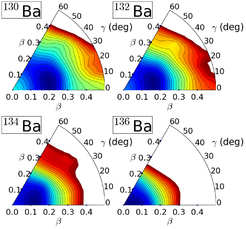
Figure 1: (Color online) Self-consistent RHB triaxial quadrupole binding energy maps of the even-even ^130-136Ba isotopes in the $\beta-\gamma$ plane ($0\leq\gamma\leq 60^{\circ}$). For each nucleus the energy surface is normalized with respect to the binding energy of the absolute minimum, and is plotted up to 10 MeV excitation energy with 0.2 MeV difference between neighboring contours.

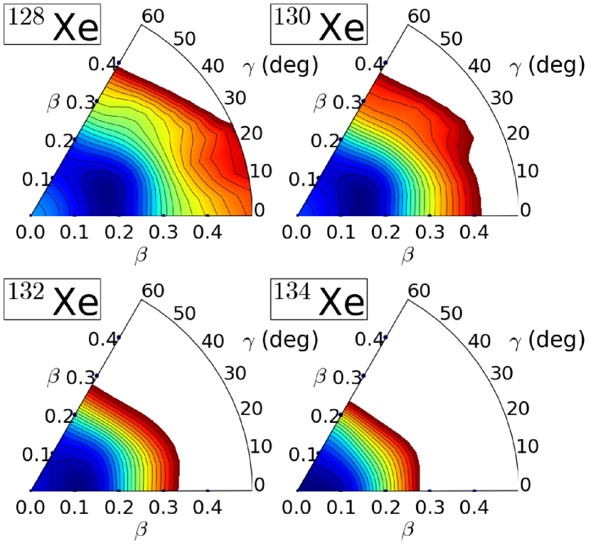
Figure 2: (Color online) Same as in the caption to Fig. 2, but for ^128-134Xe.

III.1 Deformation energy surface

As explained in the previous section, the deformation energy surfaces for a set of even-even Ba and Xe isotopes that determine the parameters of the IBM Hamiltonian, are calculated as functions of the polar deformation parameters $\beta$ and $\gamma$ Bohr and Mottelsson (1975), using the constrained relativistic Hartree-Bogoliubov method based on the functional DD-PC1 Nikšić et al. (2008) and a separable pairing force of finite range Tian et al. (2009). A triaxial binding energy map as a function of quadrupole shape variables is obtained by imposing constraints on both the axial and triaxial mass quadrupole moments. In Figs. 1 and 2, the energy surfaces for the even-even core nuclei ^130-136Ba and ^128-134Xe, respectively, are displayed in the $\beta-\gamma$ plane ($0^{\circ}\leq\gamma\leq 60^{\circ}$). We note that the energy surfaces for the ¹²⁸Ba and ¹²⁶Xe nuclei are nearly identical to those of their adjacent nuclei ¹³⁰Ba and ¹²⁸Xe, respectively, and thus are not included in the figures.

At the self-consistent mean-field level the RHB energy surfaces display a gradual transition of equilibrium shapes as a function of the (valence) neutron number. One notices that the RHB energy surfaces for the Ba and Xe isotopes are very similar and, for this reason, we discuss only the results for the Ba isotopes. As shown in Fig. 1, the shape is noticeably soft in $\gamma$ deformation for ^130,132Ba with a very shallow triaxial minimum in the interval $\gamma=10^{\circ}-20^{\circ}$. As the number of valence nucleons (neutron holes) decreases for ¹³⁴Ba, the potential appears to become almost completely flat in $\gamma$ direction, which is a typical feature of transitional nuclei. ¹³⁶Ba displays a nearly spherical shape with a minimum at $\beta\approx 0.1$, reflecting the $N=82$ neutron shell closure. It is interesting that the equilibrium shapes for the Ba nuclei display no significant change in the axial deformation $\beta$ as a function of the neutron number. We also note that the RHB energy surfaces for the Xe isotopes appear to be somewhat softer in $\gamma$ when compared to the corresponding Ba neighbors.

In the present analysis we are particularly interested in transitional nuclei. ¹³⁴Ba is located between the nearly spherical shapes close to $N=82$ and the $\gamma$-soft shapes of lighter isotopes. This nucleus was analyzed as the first empirical realization Casten and Zamfir (2000) of the critical point of second-order QPT between spherical and $\gamma$-soft shapes, described by the E(5) symmetry Iachello (2000). This symmetry corresponds to the five-dimensional collective Hamiltonian (the intrinsic variables $\beta$ and $\gamma$ and the three Euler angles), with an infinite square-well potential in the axial deformation $\beta$, and independent of $\gamma$ Iachello (2000). One notices that the microscopic deformation energy surface of ¹³⁴Ba in the present calculation is closest to the E(5)-like potential: it is flat-bottomed for small values of the axial deformation $\beta<0.2$, and almost completely flat in the $\gamma$ direction. A similar shape is predicted for ¹³²Xe.

III.2 Low-energy excitation spectra

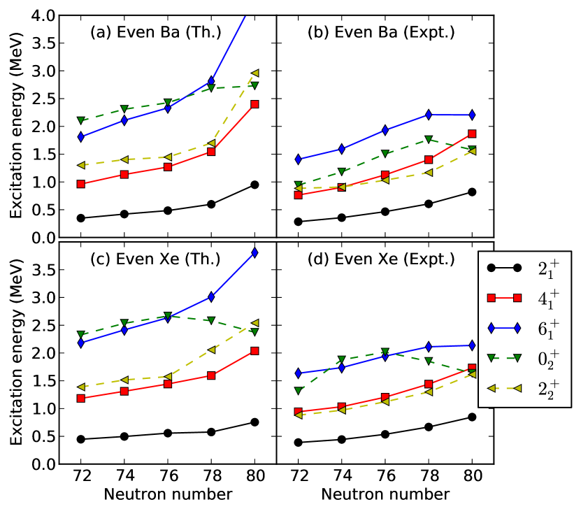
Figure 3: (Color online) Evolution of low-lying collective states in ^128-136Ba and ^126-134Xe, as functions of the neutron number. Theoretical excitation spectra in the left column are compared to data (panels on the right) from Ref. Brookhaven National Nuclear Data Center .

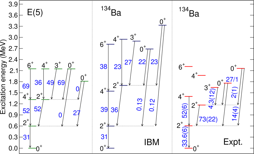
Figure 4: (Color online) The low-energy spectrum of ¹³⁴Ba calculated with the microscopic IBM, in comparison to available data Brookhaven National Nuclear Data Center ; Casten and Zamfir (2001). The excitation spectrum that corresponds to the E(5) symmetry limit is also displayed, with the excitation energy of the state $2^{+}_{1}$ and the $B(E2;2^{+}_{1}\rightarrow 0^{+}_{1})$ transition strength normalized to the values obtained in the IBM calculation.

A QPT is characterized by a significant variation of order parameters as functions of the physical control parameter. While the analysis of potential energy surfaces provides an approximate indication of QPT at the mean-field level, the intrinsic deformation parameters are not observables and a quantitative analysis of the nuclear phase transitions must, therefore, extend beyond the simple Landau approach to include a direct calculation of observables that can be interpreted as quantum order parameters.

To illustrate the level of accuracy with which the boson-core Hamiltonian, with parameters determined by mapping the microscopic energy surface onto the expectation value of the IBM Hamiltonian, describes spectroscopic properties of even-even systems, we begin by comparing in Fig. 3 the computed excitation spectra for the low-lying states of the even-even ^128-136Ba and ^126-134Xe isotopes to available data Brookhaven National Nuclear Data Center . Evidently the model calculation reproduces the empirical systematics of low-lying excitation spectra. In particular, the $\gamma$-softness of the effective nuclear potential is characterized by close-lying $4^{+}_{1}$ and $2^{+}_{2}$ levels. Both experimentally and in model calculations, this level structure is observed from $N=72$ up to 78. At $N=80$ the energy spacings correspond to vibrational spectra, as identified by the multiplets of levels $(4^{+}_{1},2^{+}_{2},0^{+}_{2})$. Overall, the theoretical excitation spectra are more stretched than the experimental ones, especially at $N=80$. This could be attributed to the limited IBM configuration space consisting only of the valence nucleon pairs outside closed shells.

¹³⁴Ba is considered an excellent example of empirical realization of the E(5) critical-point symmetry Casten and Zamfir (2000). In Fig. 4 we compare the calculated energy spectrum of this nucleus with the experimental low-energy levels, as well as with the spectrum corresponding to the E(5) symmetry limit. In comparison to the experimental levels, the present calculation generally predicts higher excitation energies, but exhibits several features that correspond to the E(5) symmetry, including the close-lying ($4^{+}_{1},2^{+}_{2}$) and ($6^{+}_{1},4^{+}_{2},3^{+}_{1},0^{+}_{2}$) levels, as well as the selection rule for E2 transitions from the $0^{+}_{2}$ to the $2^{+}_{1,2}$ states.

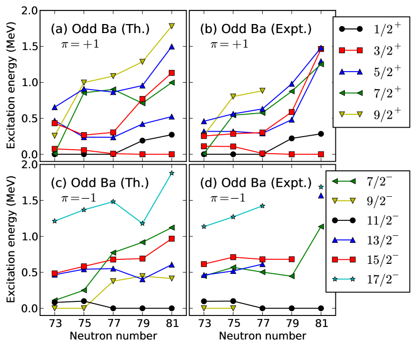
Figure 5: (Color online) Evolution of the low-lying positive- and negative-parity states in the odd-A isotopes ^129-137Ba as functions of the neutron number. The experimental levels are from Ref. Brookhaven National Nuclear Data Center .

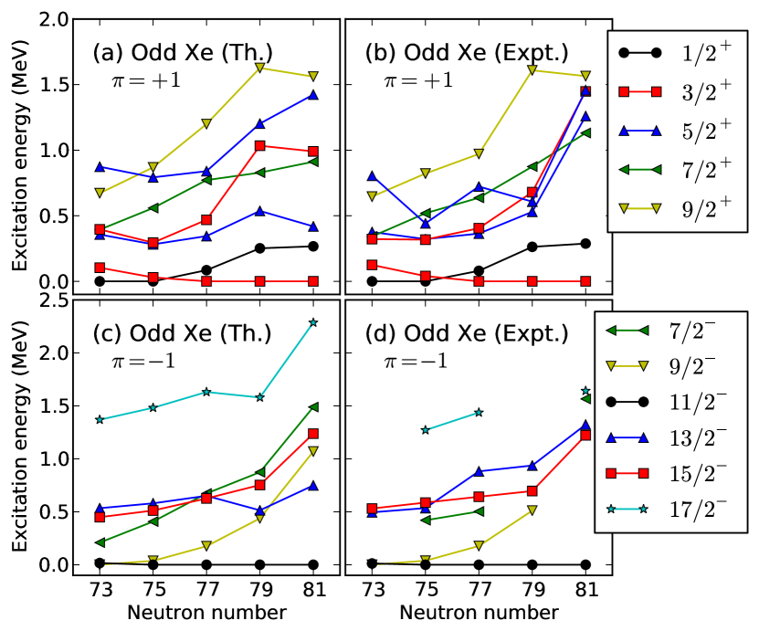
Figure 6: (Color online) Same as in the caption to Fig. 5, but for the isotopes ^127-135Xe.

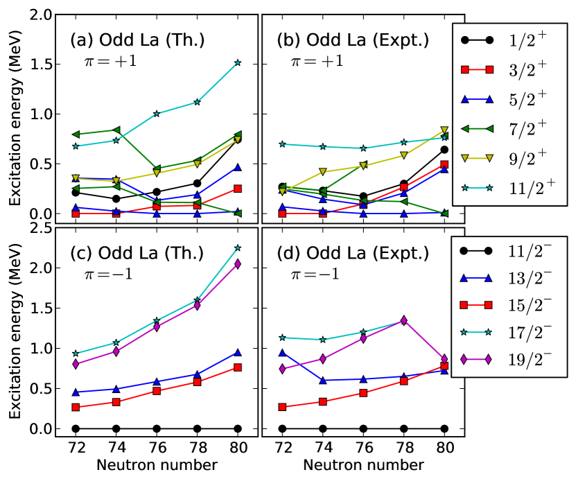
Figure 7: (Color online) Same as in the caption to Fig. 5, but for ^129-137La.

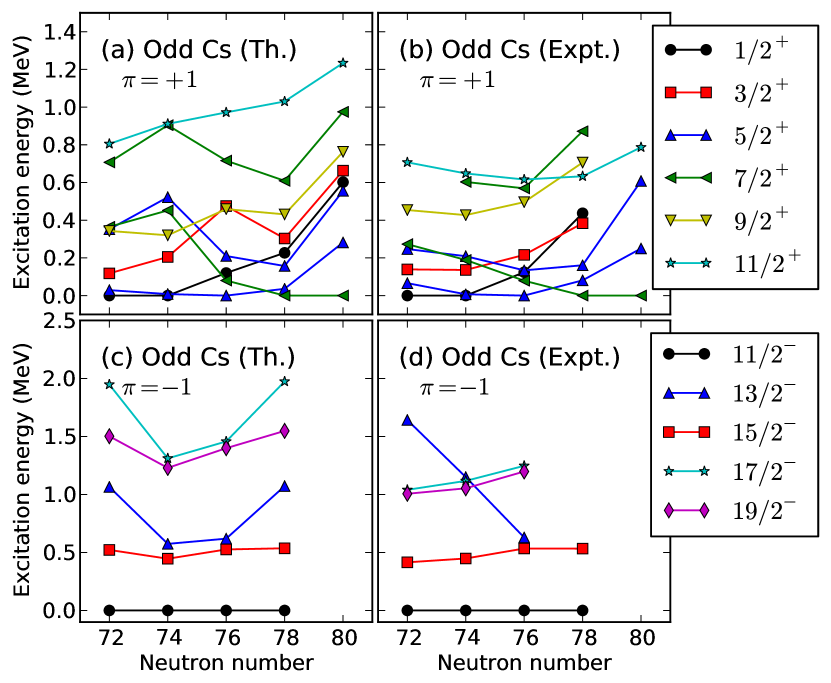
Figure 8: (Color online) Same as in the caption to Fig. 5, but for ^127-135Cs.

In the following we focus the analysis on the results for odd-A systems. Figures 5-8 display the calculated low-energy positive ($\pi=+1$) and negative-parity ($\pi=-1$) levels of the odd-A isotopes ^129-137Ba, ^127-135Xe, ^129-137La and ^127-135Cs, respectively, as functions of the neutron number, in comparison with the experimental excitation spectra Brookhaven National Nuclear Data Center . We note a remarkable agreement between theory and experiment for both $\pi=+1$ and $\pi=-1$ states in all four isotopic chains.

A specific signature of QPT in odd-A nuclei is the change of the ground-state spin at a nucleon number that corresponds to the phase transition. For the odd-A Ba isotopes show in Fig. 5, for instance, the spin of the lowest positive-parity state changes from $J^{\pi}={1/2}^{+}$ to ${3/2}^{+}$ at $N=79$, while the change of the lowest negative-parity state from $J^{\pi}={9/2}^{-}$ to ${11/2}^{-}$ is observed at $N=77$. This result is in agreement with the assumption that the QPT in the even-even Ba isotopes occurs at $N=78$, that is, for ¹³⁴Ba. It also illustrates the difficulty in locating the point of shape-phase transition when the physical control parameter (neutron number in this case) is not continuous. One also notices in Figs. 5 (a) and (b) that, compared to the other odd-A Ba isotopes considered, the ${7/2}^{+}_{1}$ and ${9/2}^{+}_{1}$ states at $N=73$ are noticeably low in energy, almost degenerate with the ${1/2}^{+}_{1}$ ground state. Empirically, it has been suggested that these states predominantly correspond to the $1g_{7/2}$ configuration Brookhaven National Nuclear Data Center ; Cunningham (1982), reflecting the fact that the $1g_{7/2}$ single-particle orbital is particularly low at $N=73$, and close in energy to the $3s_{1/2}$ and $2d_{3/2}$ orbitals. In our analysis, the calculated wave functions of the ${7/2}^{+}_{1}$ and ${9/2}^{+}_{1}$ states are almost pure (94 and 96 %, respectively) $1g_{7/2}$ configurations, which conforms to the empirical interpretation of these states. Figure 6 displays a similar pattern for the odd-A Xe isotopes, except that in this case the change in spin of the lowest positive and negative parity states occurs already at $N=77$ and $N=75$, respectively.

In the odd-Z systems ^129-137La (Fig. 7) and ^127-135Cs (Fig. 8), on the one hand we notice the crossings between low-energy positive-parity levels in the transitional region between $N=76$ and $N=78$. On the other hand, the negative-parity states of both odd-A La and Cs isotopes exhibit essentially the same level structure throughout the isotopic chains, that is, the band built on the ${11/2}^{-}$ state that follows the $\Delta J=2$ systematics of the weak coupling limit.

III.3 Detailed level schemes of selected odd-A nuclei

The details of the IBFM results are illustrated for one odd-A nucleus of each isotopic chain: ¹³⁵Ba, ¹²⁹Xe, ¹³³La, and ¹³¹Cs. These specific nuclei are close to the shape-phase transition point, their low-energy level sequences are experimentally well established, and there is sufficient data to compare with model results, especially for the $E2$ and $M1$ transitions, as well as spectroscopic moments. Note that the calculated levels are classified into bands according to the dominant E2 decay branch.

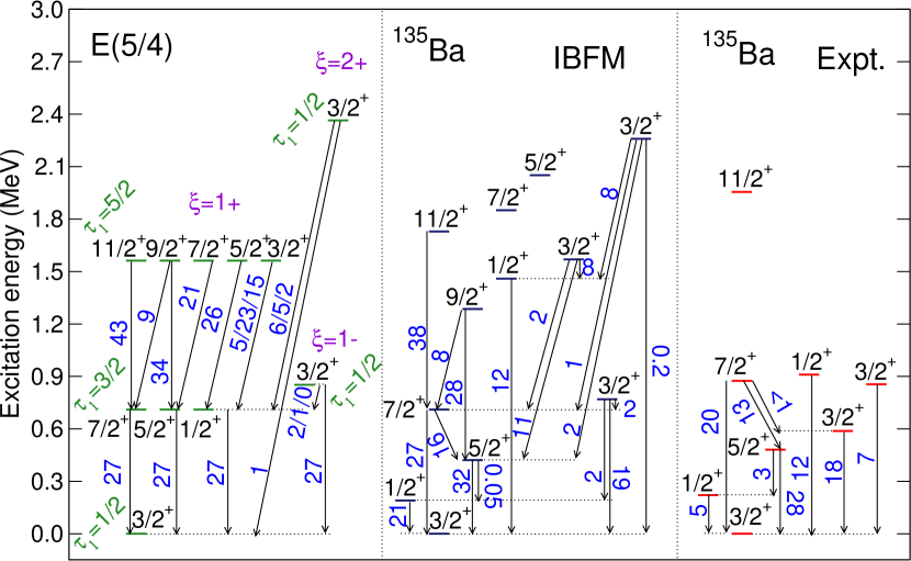
Figure 9: (Color online) The calculated low-energy positive-parity spectrum of ¹³⁵Ba (IBFM), compared to the corresponding experimental Fetea et al. (2006) and E(5/4) excitation spectra. The quantum numbers of the E(5/4) model are also shown. Note that the energy of the $(\xi=1+,\tau_{1}={3/2})$ E(5/4) multiplet, i.e., (${7/2}^{+}$, ${5/2}^{+}$, ${1/2}^{+}$), is normalized to that of the ${7/2}^{+}_{1}$ IBFM state. $B(E2)$ values are given in Weisskopf units, and the $B(E2)$ from the $(\xi=1+,\tau_{1}={3/2})$ E(5/4) multiplet is normalized to the $B(E2;{7/2}^{+}_{1}\rightarrow{3/2}^{+}_{1})$ value obtained in the present IBFM calculation. The triplets of $B(E2)$ values in the E(5/4) model spectrum refer to transitions to the ${7/2}^{+}_{1}$, ${5/2}^{+}_{1}$, and ${1/2}^{+}_{1}$ states, respectively.

¹³⁵Ba is of particular interest in the present analysis, since the corresponding even-even core ¹³⁴Ba can be, to a good approximation, characterized by the E(5) critical-point symmetry of the second-order QPT. In Ref. Iachello (2005) the E(5/4) model of critical-point symmetry for odd-mass systems was developed, based on the concept of dynamical supersymmetry. The E(5/4) model describes the coupling of an unpaired $j={3/2}$ nucleon to the even-even boson core with E(5) symmetry. In fact, the first test of the E(5/4) Bose-Fermi symmetry Fetea et al. (2006) considered the low-energy spectrum of ¹³⁵Ba in terms of the neutron $2d_{3/2}$ orbital coupled to the E(5) boson core ¹³⁴Ba. In Fig. 9 we compare the IBFM low-energy positive-parity spectrum of ¹³⁵Ba and the corresponding $B(E2)$ values with the predictions of the E(5/4) model, as well as with the experimental excitation spectrum Fetea et al. (2006). Evidently the E(5/4) spectrum is more regular, that is, it displays degenerate multiplets of excited states, when compared to both the present IBFM and experimental energy spectra. Moreover, the E2 branching ratios of the E(5/4) model, e.g., from the excited ${3/2}^{+}$ states, differ from those obtained in the present calculation. This is not surprising because E(5/4) presents a simple scheme that takes into account only a single neutron valence orbit $2d_{3/2}$. In the phenomenological IBFM calculation that was carried out in Ref. Fetea et al. (2006), the wave functions of the ${1/2}^{+}_{1}$ and ${1/2}^{+}_{2}$ states were found to be mainly composed of the $3s_{1/2}$ and $2d_{3/2}$ configurations, respectively, and it was thus suggested that the ${1/2}^{+}_{1}$ state in the first excited E(5/4) multiplet should be compared with the experimental ${1/2}^{+}_{2}$ state. Similar results are also obtained in the present calculation, as the $3s_{1/2}$ and $2d_{3/2}$ configurations account for 58% and 78% of the wave functions of the ${1/2}^{+}_{1}$ and ${1/2}^{+}_{2}$ states, respectively.

The present IBFM results reproduce the experimental excitation spectrum rather well, except for the fact that several non-yrast states, such as ${1/2}^{+}_{2}$, are calculated at higher excitation energies. In Tab. 6 we also compare in detail the calculated $B(E2)$ and $B(M1)$ transition strengths, as well as the spectroscopic quadrupole ($Q_{J}$) and magnetic ($\mu_{J}$) moments, with available data Brookhaven National Nuclear Data Center . Considering the complexity of the level scheme and the large valence neutron space, a relatively good agreement is obtained between the calculated and experimental electromagnetic properties.

Table 6: Comparison between the theoretical and experimental $B(E2)$ and $B(M1)$ values, and spectroscopic quadrupole and magnetic moments in ¹³⁵Ba. The data are from Ref. Brookhaven National Nuclear Data Center .

	$B(E2)$ (W.u.)		$B(M1)$ (W.u.)
	Th.	Expt.	Th.	Expt.
${1/2}^{+}_{1}\rightarrow{3/2}^{+}_{1}$	21	4.6(2)	0.0014	0.0025(11)
${1/2}^{+}_{2}\rightarrow{3/2}^{+}_{1}$	12	11.7(10)	-	-
${3/2}^{+}_{2}\rightarrow{3/2}^{+}_{1}$	2.0	18.0(10)	-	-
${3/2}^{+}_{3}\rightarrow{3/2}^{+}_{1}$	4.6	7.0(10)	-	-
${5/2}^{+}_{1}\rightarrow{1/2}^{+}_{1}$	0.05	2.6(5)	-	-
${5/2}^{+}_{1}\rightarrow{3/2}^{+}_{1}$	32	28.3(10)	0.0012	0.0042(20)
${7/2}^{+}_{1}\rightarrow{3/2}^{+}_{1}$	27	19.9(8)	-	-
${7/2}^{+}_{1}\rightarrow{5/2}^{+}_{1}$	16	12.8(12)	0.0020	0.0032(3)
	$Q_{J}$ ($e$b)		$\mu_{J}$ ($\mu_{N}^{2}$)
	Th.	Expt.	Th.	Expt.
${3/2}^{+}_{1}$	+0.475	+0.160(3)	+0.769	+0.837943(17)
${11/2}^{-}_{1}$	+1.13	+0.98(8)	-1.161	-1.001(15)

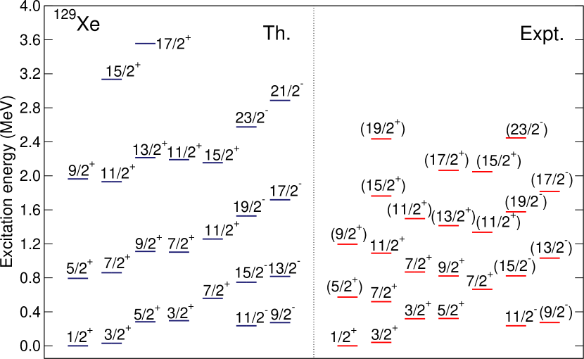
Figure 10: (Color online) Comparison between the IBFM theoretical and experimental Brookhaven National Nuclear Data Center lowest-lying positive- and negative-parity bands of ¹²⁹Xe.

In Fig. 10 we display a detailed comparison between the IBFM theoretical and experimental Brookhaven National Nuclear Data Center lowest-lying positive- and negative-parity bands of ¹²⁹Xe. For both parities the present calculation reproduces the structure of the experimental bands, especially the band-head energies. The low-energy positive- and negative-parity bands, both theoretical and experimental, exhibit a $\Delta J=2$ systematics characteristic of the weak coupling limit. The theoretical positive-parity bands are generally more stretched than the experimental ones, whereas a very good agreement between theory and experiment is obtained for the two negative-parity bands. Table 7 compares the calculated and experimental $B(E2)$ and $B(M1)$ values, as well as the electromagnetic moments of ¹²⁹Xe.

Table 7: Same as in the caption to Tab. 6, but for ¹²⁹Xe.

	$B(E2)$ (W.u.)		$B(M1)$ (W.u.)
	Th.	Expt.	Th.	Expt.
${1/2}^{+}_{2}\rightarrow{1/2}^{+}_{1}$	-	-	0.010	0.0016(5)
${1/2}^{+}_{2}\rightarrow{3/2}^{+}_{1}$	22	6.7(23)	0.049	0.0039(13)
${1/2}^{+}_{2}\rightarrow{3/2}^{+}_{2}$	-	-	0.0039	0.0015(5)
${1/2}^{+}_{2}\rightarrow{5/2}^{+}_{1}$	0.018	1.4(6)	-	-
${3/2}^{+}_{1}\rightarrow{1/2}^{+}_{1}$	0.89	9(4)	0.0019	0.0281(7)
${3/2}^{+}_{2}\rightarrow{1/2}^{+}_{1}$	33	23${}^{+25}_{-23}$	-	-
${3/2}^{+}_{2}\rightarrow{3/2}^{+}_{1}$	16	17${}^{+27}_{-17}$	0.00091	0.003${}^{+4}_{-3}$
${3/2}^{+}_{3}\rightarrow{1/2}^{+}_{1}$	7.4	$>$0.2	0.016	$>$0.0001
${3/2}^{+}_{3}\rightarrow{1/2}^{+}_{2}$	8.1	$>$5.9	0.017	$>$0.0026
${3/2}^{+}_{3}\rightarrow{3/2}^{+}_{1}$	9.2	$>$1.6	0.0027	$>$0.00071
${3/2}^{+}_{3}\rightarrow{3/2}^{+}_{2}$	0.16	$>$3.4	0.029	$>$0.00037
${3/2}^{+}_{3}\rightarrow{5/2}^{+}_{1}$	0.25	$>$4.6	0.00054	$>$0.0005
${5/2}^{+}_{1}\rightarrow{1/2}^{+}_{1}$	13	21(4)	-	-
${5/2}^{+}_{1}\rightarrow{3/2}^{+}_{1}$	46	5${\times}10^{1}$(4)	0.0013	0.011(5)
${5/2}^{+}_{4}\rightarrow{1/2}^{+}_{1}$	2.0	15.4(19)	-	-
	$Q_{J}$ ($e$b)		$\mu_{J}$ ($\mu_{N}^{2}$)
	Th.	Expt.	Th.	Expt.
${1/2}^{+}_{1}$	-	-	-1.126	-0.7779763(84)
${3/2}^{+}_{1}$	+0.362	-0.393(10)	+0.72	+0.58(8)
${11/2}^{-}_{1}$	+0.092	+0.63(2)	-1.247	-0.891223(4)

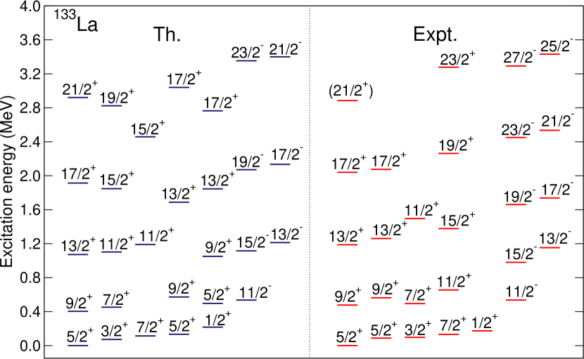
Figure 11: (Color online) Same as in the caption to Fig. 10, but for ¹³³La.

Next we consider the two odd-Z nuclei, for which the low-lying states predominantly correspond to the $1g_{7/2}$, $2d_{5/2}$ (positive-parity) and $1h_{11/2}$ (negative-parity) proton configurations. Figure 11 compares several calculated low-energy positive- and negative-parity bands of ¹³³La with available data. One notices a good agreement between the theoretical and experimental excitation spectra, except for that fact that some of the calculated bands, that is, the band built on the ${7/2}^{+}_{1}$ state and the two negative-parity bands, appear more stretched than their experimental counterparts. Similar to ¹²⁹Xe, all the low-energy positive- and negative-parity bands shown here exhibit a $\Delta J=2$ weak-coupling structure. The calculated and experimental $B(E2)$ and $B(M1)$ values, as well as the electromagnetic moments are listed in Tab. 8.

Table 8: Same as in the caption to Tab. 6, but for ¹³³La.

	$B(E2)$ (W.u.)		$B(M1)$ (W.u.)
	Th.	Expt.	Th.	Expt.
${1/2}^{+}_{1}\rightarrow{3/2}^{+}_{1}$	9.4	6(3)	0.77	0.017(6)
${1/2}^{+}_{1}\rightarrow{5/2}^{+}_{1}$	30	0.8(3)	-	-
${3/2}^{+}_{1}\rightarrow{5/2}^{+}_{1}$	26	$>$35	0.13	$>$0.026
${5/2}^{+}_{2}\rightarrow{5/2}^{+}_{1}$	15	2.1(10)	0.13	0.0097(8)
${7/2}^{+}_{1}\rightarrow{5/2}^{+}_{1}$	18	11(4)	0.00011	0.0052(9)
${7/2}^{+}_{1}\rightarrow{5/2}^{+}_{2}$	21	6.1(20)	1.0$\times 10^{-5}$	0.00068(16)
	$Q_{J}$ ($e$b)		$\mu_{J}$ ($\mu_{N}^{2}$)
	Th.	Expt.	Th.	Expt.
${11/2}^{-}_{1}$	-	-	+6.9	+7.5(4)

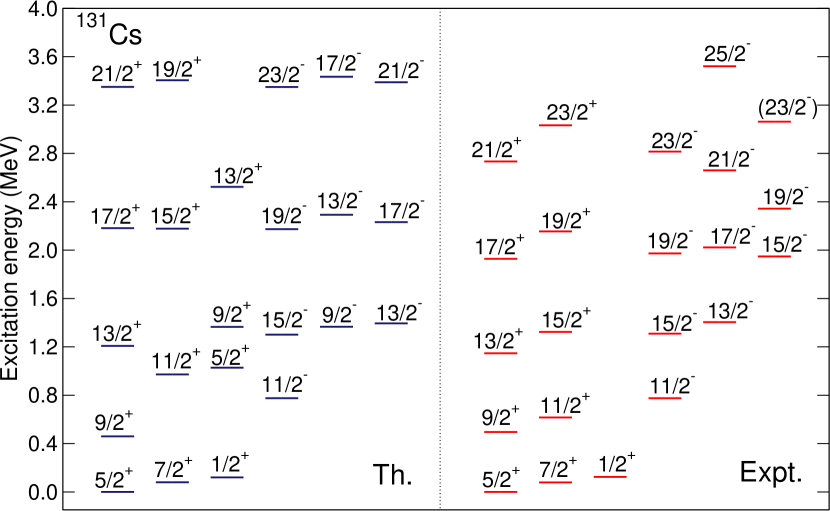
Figure 12: (Color online) Same as in the caption to Fig. 10, but for ¹³¹Cs.

The theoretical excitation spectrum of ¹³¹Cs, shown in Fig, 12, is very similar to that of ¹³³La and, again, a very good agreement is obtained between the IBFM results and experiment. The calculated E2 and M1 transition strengths and electromagnetic moments are compared with the data Brookhaven National Nuclear Data Center in Tab. 9. We note that the model calculation qualitatively reproduces the complex transition pattern, but obviously the theoretical wave functions do not reflect the full extent of configuration mixing in this nucleus.

Table 9: Same as in the caption to Tab. 6, but for ¹³¹Cs. Note that the sign is not known for the experimental $Q_{{5/2}^{+}_{2}}$ and $\mu_{{11/2}^{-}_{1}}$.

	$B(E2)$ (W.u.)		$B(M1)$ (W.u.)
	Th.	Expt.	Th.	Expt.
${1/2}^{+}_{1}\rightarrow{5/2}^{+}_{1}$	59	69.5(14)	-	-
${1/2}^{+}_{2}\rightarrow{1/2}^{+}_{1}$	-	-	0.013	0.0010613(4)
${1/2}^{+}_{2}\rightarrow{3/2}^{+}_{1}$	1.7	0.09(4)	0.011	$3.4\times 10^{-5}(10)$
${1/2}^{+}_{2}\rightarrow{3/2}^{+}_{2}$	38	$>$0.62	0.0064	$>5.8\times 10^{-5}$
${1/2}^{+}_{2}\rightarrow{5/2}^{+}_{1}$	0.19	0.028248(4)	-	-
${1/2}^{+}_{2}\rightarrow{5/2}^{+}_{2}$	4.7	0.13835(5)	-	-
${3/2}^{+}_{1}\rightarrow{1/2}^{+}_{1}$	18	9(5)	0.30	0.00339(10)
${3/2}^{+}_{1}\rightarrow{5/2}^{+}_{1}$	12	0.6(6)	0.22	0.00922(5)
${3/2}^{+}_{1}\rightarrow{5/2}^{+}_{2}$	0.27	$>$3.9	0.0022	$>4.1^{-5}$
${3/2}^{+}_{1}\rightarrow{7/2}^{+}_{1}$	1.4	2.36(3)	-	-
${3/2}^{+}_{2}\rightarrow{1/2}^{+}_{1}$	0.94	2.4(4)	0.018	0.00057(4)
${3/2}^{+}_{2}\rightarrow{3/2}^{+}_{1}$	0.012	$>$2.1	2.7$\times 10^{-5}$	$>7.8\times 10^{-5}$
${3/2}^{+}_{2}\rightarrow{5/2}^{+}_{1}$	0.55	2.4(9)	0.0012	0.00064(20)
${3/2}^{+}_{2}\rightarrow{5/2}^{+}_{2}$	0.63	0.5(4)	0.0014	0.00071(4)
${3/2}^{+}_{2}\rightarrow{7/2}^{+}_{1}$	25	0.2122(3)	-	-
${5/2}^{+}_{2}\rightarrow{5/2}^{+}_{1}$	0.016	3.5(3)	0.0036	0.000369(17)
${5/2}^{+}_{2}\rightarrow{7/2}^{+}_{1}$	45	$>$62	3.1$\times 10^{-5}$	$<2.1\times 10^{-5}$
${7/2}^{+}_{1}\rightarrow{5/2}^{+}_{1}$	0.10	0.64(24)	0.0010	0.00170(5)
	$Q_{J}$ ($e$b)		$\mu_{J}$ ($\mu_{N}^{2}$)
	Th.	Expt.	Th.	Expt.
${5/2}^{+}_{1}$	-0.772	-0.575(6)	+3.42	+3.543(2)
${5/2}^{+}_{2}$	+0.370	0.022(2)	+0.37	+1.86(8)
${11/2}^{-}_{1}$	-	-	+6.9	6.3(9)

III.4 Effective $\beta$ and $\gamma$ deformations

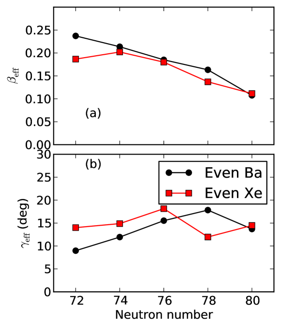
Figure 13: (Color online) $\beta_{\rm eff}$ and $\gamma_{\rm eff}$ for the $0^{+}_{1}$ state of the even-even ^128-136Ba and ^126-134Xe isotopes, obtained from the computed q-invariants.

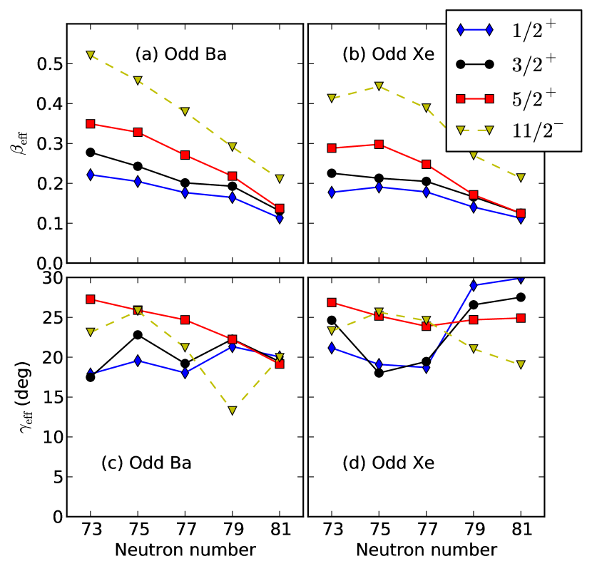
Figure 14: (Color online) Same as in the caption to Fig. 13, but for the ${1/2}^{+}_{1}$, ${3/2}^{+}_{1}$, ${5/2}^{+}_{1}$ and ${11/2}^{-}_{1}$ states of the odd-N ^129-137Ba and ^127-135Xe isotopes.

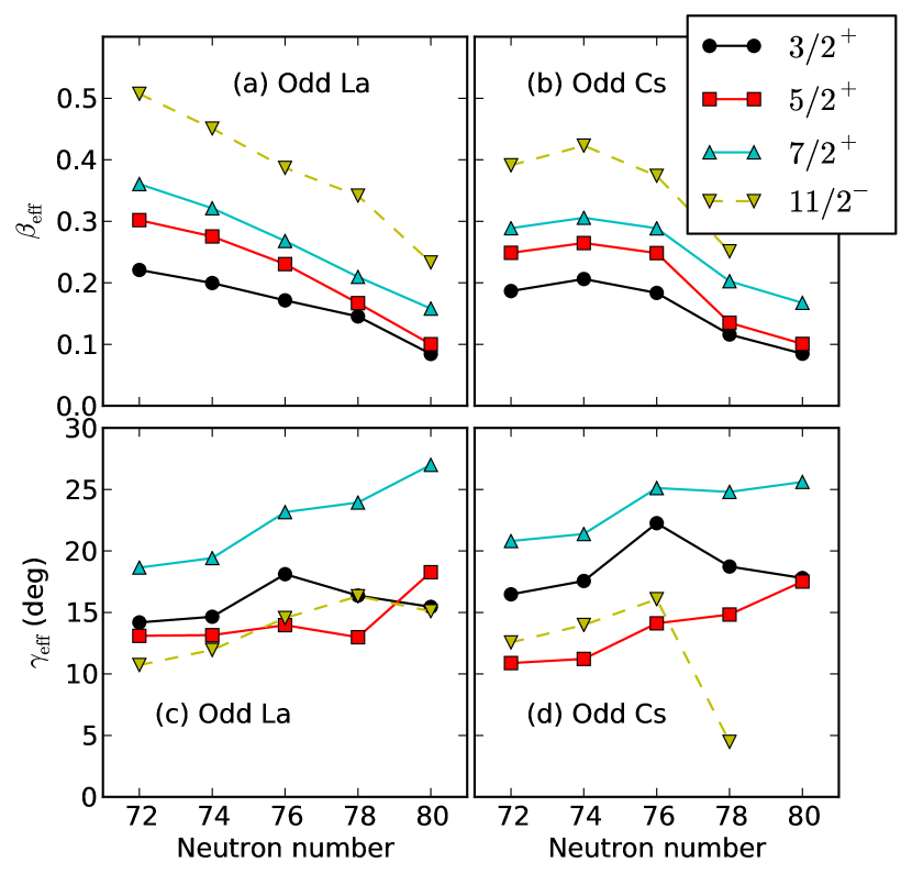
Figure 15: (Color online) Same as in the caption to Fig. 13, but for the ${3/2}^{+}_{1}$, ${5/2}^{+}_{1}$, ${7/2}^{+}_{1}$ and ${11/2}^{-}_{1}$ states of the odd-Z ^129-137La and ^127-135Cs isotopes.

Another signature of possible shape-phase transitions related to the $\gamma$-softness of the effective nuclear potential, can be computed from $E2$ transition rates. Here we specifically analyze quadrupole shape invariants Cline (1986) (denoted hereafter as q-invariants), calculated using $E2$ matrix elements. The lowest-order q-invariants for a given state with spin $J$, relevant for the present study, are defined by the following relations Werner et al. (2000):

$$q_{2}=\sum_{i}^{n}\langle J||\hat{Q}||J^{\prime}_{i}\rangle\langle J^{\prime}_{i}||\hat{Q}||J\rangle$$ (15)

$$q_{3}=\sqrt{\frac{7}{10}}|\sum_{i,j}^{n}\langle J||\hat{Q}||J^{\prime}_{i}\rangle\langle J^{\prime}_{i}||\hat{Q}||J^{\prime}_{j}\rangle\langle J^{\prime}_{j}||\hat{Q}||J\rangle|$$ (16)

where $J^{\prime}=J+2$, and the sum is in order of increasing excitation energies of the levels $J^{\prime}$. Only a few lowest transitions contribute to the q-invariants significantly and, in the present study, the sum runs up to $n=5$. For even-even systems, we calculate the q-invariants for the $0^{+}_{1}$ ground state, which means $J=0^{+}_{1}$ and $J^{\prime}=2^{+}$. The effective deformation parameters, denoted as $\beta_{\rm eff}$ and $\gamma_{\rm eff}$, can be obtained from $q_{2}$ and $q_{3}$ Werner et al. (2000):

$$\beta_{\rm eff}=\frac{4\pi}{3ZR^{2}_{0}}\sqrt{\frac{q_{2}}{2J^{\prime}+1}(J^{\prime}2J0|JJ)^{-2}}$$ (17)

$$\gamma_{\rm eff}=\frac{1}{3}\arccos{\frac{q_{3}}{q_{2}^{3/2}}}$$ (18)

where $R_{0}=1.2A^{1/3}$ fm, and $(J^{\prime}2J0|JJ)$ is the Clebsch-Gordan coefficient.

In Fig. 13 we plot $\beta_{\rm eff}$ and $\gamma_{\rm eff}$ for the even-even isotopes ^128-136Ba and ^126-134Xe, as functions of the neutron number. One notices that, both for Ba and Xe nuclei, $\beta_{\rm eff}$ exhibits only a gradual decrease with neutron number. This correlates with the mean-field result, which indicates that the $\beta$ deformation does not change significantly as a function of neutron number (cf. Figures 1 and 2). In contrast, $\gamma_{\rm eff}$ displays a distinct peak at $N=78$ for Ba and at $N=76$ for Xe, which could be associated with the phase transition between nearly spherical and prominently $\gamma$-soft shapes. Indeed, the deformation energy surface at around these neutron numbers resembles the potential in the E(5) model, which is flat-bottomed in an interval of the axial deformation $\beta$, and independent of $\gamma$.

In the case of odd-A nuclei the spin of the ground state is not always the same for all isotopes, and we have thus calculated $\beta_{\rm eff}$ and $\gamma_{\rm eff}$ for several low-lying state. Figure 14 displays $\beta_{\rm eff}$ and $\gamma_{\rm eff}$ of the states ${1/2}^{+}_{1}$, ${3/2}^{+}_{1}$, ${5/2}^{+}_{1}$ and ${11/2}^{-}_{1}$ for the odd-N systems, that is, ^127-135Xe and ^129-137Ba. Similarly to the corresponding even-even core nuclei, in the odd-A Ba nuclei shown in Fig. 14 (a) for all four states $\beta_{\rm eff}$ exhibits only a gradual decrease with the neutron number. For the states ${5/2}^{+}_{1}$ and ${11/2}^{-}_{1}$ in the odd-Xe nuclei, however, $\beta_{\rm eff}$ indicates a discontinuity at $N=75$. $\gamma_{\rm eff}$, shown in Figs. 14 (c) and (d), exhibits a significant change (either increase or decrease) for many states at $N=79$. In addition, $\gamma_{\rm eff}$ for the states ${3/2}^{+}_{1}$ and ${5/2}^{+}_{1}$ of odd-A Ba nuclei displays another variation at $N=75$. Similar results are also obtained for the odd-Z La and Cs nuclei, as shown in Fig. 15. However, $\gamma_{\rm eff}$ for the odd-Z La and Cs isotopes exhibits a more pronounced signature of shape phase transition when compared to the odd-N Ba and Xe nuclei: a significant change at $N=76$ or 78 for the odd-A La, and at $N=76$ for the odd-A Cs isotopes.

IV Concluding remarks

Using the recently proposed method of Ref. Nomura et al. (2016a), based on the microscopic framework of nuclear energy density functionals and the particle-core coupling scheme, we have analyzed signatures of QPTs in $\gamma$-soft odd-mass nuclei with mass $A\approx 130$. The deformation energy surface of the even-even core nuclei, and the spherical single-particle energies and occupation probabilities of the unpaired nucleon, are obtained by relativistic Hartree-Bogoliubov SCMF calculations with a specific choice of the energy density functional and pairing interaction.

The microscopic SCMF calculations determine the parameters of boson and fermion Hamiltonians used to model spectroscopic properties of the odd-A ^129-137Ba, ^127-135Xe, ^129-137La and ^127-135Cs nuclei, whereas the strength parameters of the particle-core coupling are adjusted to reproduce selected empirical results of low-energy spectra in odd-A systems. The method provides a very good description of spectroscopic properties of the $\gamma$-soft odd-mass systems. Even though phase transitions are smoothed out in finite systems, especially a second-order QPT as the one considered here, and the physical control parameter takes only integer values (the nucleon number), the SCMF deformation energy surfaces and the resulting excitation spectra consistently point to a shape phase transition in the interval $N=76-78$, both in even-even and odd-mass systems. In particular, $\gamma_{\rm eff}$, evaluated using E2 matrix elements for transitions between low-lying states, clearly exhibits a discontinuity near $N=76$ and 78, which signals the occurrence of a phase transition between nearly spherical and $\gamma$-soft shapes. The results obtained in this work, as well as in our previous studies on odd-A Sm and Eu Nomura et al. (2016a, b), have shown that the method of Nomura et al. (2016a) works not only in axially-deformed nuclei, but also in $\gamma$-soft or axially-asymmetric odd-mass systems, and enables a systematic investigation of the structural evolution in odd-A nuclei in medium-heavy and heavy-mass regions.

The necessity to fit the strength parameters of the boson-fermion coupling Hamiltonian to spectroscopic data in the considered odd-mass nuclei, presents a serious limitation of the current implementation of our IBF method. In contrast to the parameters of the boson and fermion Hamiltonians that are completely determined by the choice of a global EDF and pairing interaction, the boson-fermion coupling must be specifically adjusted for each odd-mass nucleus. This procedure, of course, limits the applicability to those nuclei for which enough low-energy structure data are available to completely determine the strength of the various boson-fermion interaction terms. Therefore an important step forward would be to develop a method to microscopically determine, or at least constrain, the values of the boson-fermion coupling parameters. One possibility would be to perform SCMF calculations for odd-A systems and map the resulting deformation energy surface onto the expectation value of the IBFM Hamiltonian in the boson-fermion condensate state Leviatan (1988). SCMF calculations for odd-A nuclei are, of course, computationally very challenging and such an approach would be difficult to apply in systematic studies of a large number of nuclei. Another strategy would be to derive the boson-fermion coupling from a microscopic shell-model interaction between nucleons in a given valence space Scholten and Dieperink (1981). In this approach the parameters can be determined by equating the matrix elements in the IBFM space to those in the shell-model space. The disadvantage of this method is that it requires the explicit introduction of a new building block, that is, the shell-model interaction. This is certainly an interesting problem and will be the topic of future studies and development of the semi-phenomenological model employed in the present analysis.