Data-adaptive statistics for multiple hypothesis testing in high-dimensional settings

Abstract

Current statistical inference problems in areas like astronomy, genomics, and marketing routinely involve the simultaneous testing of thousands – even millions – of null hypotheses. For high-dimensional multivariate distributions, these hypotheses may concern a wide range of parameters, with complex and unknown dependence structures among variables. In analyzing such hypothesis testing procedures, gains in efficiency and power can be achieved by performing variable reduction on the set of hypotheses prior to testing. We present in this paper an approach using data-adaptive multiple testing that serves exactly this purpose. This approach applies data mining techniques to screen the full set of covariates on equally sized partitions of the whole sample via cross-validation. This generalized screening procedure is used to create average ranks for covariates, which are then used to generate a reduced (sub)set of hypotheses, from which we compute test statistics that are subsequently subjected to standard multiple testing corrections. The principal advantage of this methodology lies in its providing valid statistical inference without the a priori specifying which hypotheses will be tested. Here, we present the theoretical details of this approach, confirm its validity via simulation study, and exemplify its use by applying it to the analysis of data on microRNA differential expression.

Key words: data mining, data-adaptive statistical target parameter, cross-validation, machine learning, targeted maximum likelihood estimation.

1 Introduction

Recently developed technologies enable high throughput screen of thousands (millions) of biological molecules, which has resulted in filters that use multiple testing to highlight potentially informative biomakers. For instance, consider microRNA, a new class of small, non-coding RNAs have been the subject of intense study due to their central role in gene regulation (Wienholds et al., 2005). In a process involving binding to messenger RNA (mRNA), miRNAs regulate gene expression at the post-transcriptional level, thereby affecting the abundance of a wide range of proteins in diverse biological processes. The resulting data consists of a large vector of microRNA expressions as well as other characteristics and experimental conditions relevant to a particular biological sample. Before looking at the complex relationship of these molecules, a first step is often examining the association of microRNA expression with some other phenotypic variable(s). In our case, we consider a study examining the relationship of occupational exposure benzene (a known carcinogen) to microRNA expression. This study, like many of its kind, has a relative small sample size, but large ambitions regarding the teasing out of associations of many thousands of potential microRNA’s. In this paper, we propose a method that adaptively reduces the number of tests so that a study can preserve reasonable power even when the number of potential tests is huge.

Speaking generally, current problems of statistical inference involving multiple hypothesis testing share the following characteristics: inference for high- dimensional multivariate distributions, with complex and unknown dependence structures among variables; a variety of parameters of interest, such as coefficients in general regression models relating possibly censored biological and clinical covariates and outcomes to genome-wide expression measures and genotypes; many null hypotheses, in the thousands or even millions; complex and unknown dependence structures among test statistics.

An often-ignored yet insidious issue with small-sample inference and large numbers of comparisons is the enormous sample sizes required for joint convergence, by the central limit theorem, of the joint sampling distribution to a multivariate normal distribution. Unfortunately, others have shown that for convergence to multivariate normal distribution in the far tails (to derive accurate adjustment for multiple testing) requires astronomical sample sizes (e.g., from high-throughput sequencing technologies). Gerlovina and Hubbard (2016) employed Edgeworth expansions to rigorously study the manner in which the number of tests performed affects the accuracy of the resultant analyses, with particular attention paid to situations where the number of tests vastly outnumbers the sample size. Here, the utility of Edgeworth series lies in their providing, by way of higher-order approximations, estimates of critical values that would otherwise be computed exactly were the true distribution known. In any case, these expansions and associated simulations of multiple testing experiments showed that error control can be wildly anti-conservative if sample size is inadequate. Thus, using standard and commonly used multiple testing techniques can make it practically impossible to obtain honest statistical inference when conducting very large numbers of tests.

Motivated by the broad use of multiple testing procedures for very large numbers of tests, and the limitations of existing multiple testing procedures, we present in this paper a technique for data-adaptive multiple testing in high-dimensional problems, one that harnesses data mining procedures to perform variable reduction, whilst preserving accurate and honest statistical inference. This new method is a natural extension of the data-adaptive statistical target parameter framework introduced by Hubbard and van der Laan (2016), who show that this new class of inference procedures provides an impetus for using methods providing rigorous statistical inference for data-mining procedures.

The proposed approach for multiple testing in high-dimensional settings uses data-adaptive test statistics, which rely on cross-validation, to perform variable reduction by screening algorithms. Typically, the method uncovers associations that represent signals that are stable across the full sample, while allowing for multiple testing efforts to be restricted to a much smaller subset of biomarkers (predictors). It is expected that this new class of test statistics outperforms, in terms of improvements in both power and control of type-I error rate, standard test statistics generated by classical approaches to multiple hypothesis testing, in which variable set is pre-specified.

In section 2, we proceed to define this methodology in generality with the aforementioned estimation strategies, present theorems establishing its asymptotic statistical performance, present influence function and bootstrap-based inference, and discuss the implications of these theoretical results. In section 3, we demonstrate the relative performance by way of simulation studies; in section 4, we apply the general approach for high-dimensional multiple testing using data-adaptive test statistics to the analysis of data from miRNA assays; and then conclude (in section 5) with remarks on the implications of this new methodology to future work in analyzing data from biomedical investigations.

2 Methodology

2.1 Notation and setup

The procedure is straightforward and involves cross-validation to keep separate the data used for choosing which tests to perform and the data used for constructing the test statistics and generating p-values. Define the observed data as $O_{i}=(W_{i},A_{i},Y_{i})\sim P_{0},i=1,...,n$, which consist of $n$ independent and identically distributed random samples from the population distribution $P_{0}$, with $P_{0}$ known to be an element of a statistical model $\mathcal{M}$. For each observation, $Y_{i}$ is the outcome of interest of dimension $p$ and can be a real number or class variable. $A_{i}$ is a 1-dimensional vector of treatment variable and $W_{i}$ is a multi-dimensional vector of baseline covariates.

Consider V-fold cross-validation, where the learning set $L$ is randomly divided into $V$ mutually exclusive and exhaustive sets, $L_{v},v=1,...,V$, of as nearly equal size as possible. We will define the parameter-generating sample for $v,L-L_{v}$, the sample used to select which of the original set of hypotheses should be considered for future testing. Then, the estimates are computed on the estimation-sample $L_{v}$, and averaged (details below) across the $v$. The proportion $p$ of observations in the estimation-sample $L_{v}$ is approximately $1/V$.

For a given random split $v$, let $P_{n,v^{c}}$ be the empirical distribution of the parameter-generating sample $L-L_{v}$, and $P_{n,v}$ be the empirical distribution of the estimation-sample $L_{v}$. ${\Psi_{{v},P_{n,v^{c}}}}:\mathcal{M}\to\mathbb{R}$ is the target parameter mapping indexed by the parameter-generating sample $P_{n,v^{c}}$, and ${\widehat{\Psi}_{{v},P_{n,v^{c}}}}:{\mathcal{M}_{NP}}\to\mathbb{R}$ the corresponding estimator of this target parameter. For instance, one might use an algorithm within the training sample to subset variables based on, say, ranking by some statistic (e.g., differential expression). Thus, ${\Psi_{{v},P_{n,v^{c}}}}$ could be the mean difference between two groups of this random subset of variables. Here, $\mathcal{M}$ is a nonparametric model and an estimator is defined as an algorithmic mapping from a nonparametric model, including all of the constituent empirical distributions, to the parameter space. For simplicity, assume that the parameter is real-valued. Thus, the target parameter mapping and estimator can depend not only on the parameter-generating sample ${P_{n,v^{c}}}$, but also on the particular split $v$.

Assume the existence of a mapping from the parameter-generating sample ${P_{n,v^{c}}}$ into a target parameter mapping and a corresponding estimator of that target parameter. The choice of target parameter mapping and corresponding estimator can be informed by the data ${P_{n,v^{c}}}$ but not by the estimation sample ${P_{n,v}}$ – that is, one only need know the realization of the mapping from the parameter-generating sample to the space of target parameter mappings and estimators $\left({{\Psi_{{v},P_{n,v^{c}}}},{{\widehat{\Psi}}_{{v},P_{n,v^{c}}}}}\right)$, but not the explicit definition of said mapping.

Define the sample-split data-adaptive statistical target parameter as ${\Psi_{n}}:\mathcal{M}\to\mathbb{R}$ with

$${\Psi_{n}}\left(P\right)={E_{{v}}}{\Psi_{{v},P_{n,v^{c}}}}\left(P\right)$$

and the statistical estimand of interest is thus

$${\Psi_{n,0}}={\Psi_{n}}\left(P_{0}\right)={E_{{v}}}{\Psi_{{v},P_{n,v^{c}}}}\left({{P_{0}}}\right)=\underset{v}{Ave}\Psi_{{v},P_{n,v^{c}}}\left(P_{0}\right).$$

Note that this target parameter mapping depends on the data, which is the reason for calling it a data-adaptive target parameter. A corresponding estimator of the data-adaptive estimand ${\Psi_{n,0}}$ is given by:

$${\Psi_{n}}=\Psi\left({{P_{n}}}\right)={E_{{v}}}{\Psi_{{v},P_{n,v^{c}}}}\left({P_{n,v}}\right).$$

2.2 Data-adaptive test statistics

In this section, we consider a rank-based approach to generate a test statistic on a reduced set of responses ${S^{0}}\subset Y$, where $S^{0}$ is a subset of the full observed data determined by the application of a selection procedure on the parameter-generating sample. The data-adaptive statistic is identified by three components: the cardinality of the reduced set denoted by ${p^{*}}\triangleq\left|{{S^{0}}}\right|$, the parameter-generating algorithm, and the number of folds $V$ in cross-validation.

Specifically, for each parameter-generating sample $L-L_{v}$, we simply rank by ${\widehat{B}_{j}}={E_{P_{n,v^{c}}}}\left({\left.{{Y_{j}}}\right|A=1}\right)-{E_{P_{n,v^{c}}}}\left({\left.{{Y_{j}}}\right|A=0}\right)$, which is the empirical average treatment effect of $A$ on $Y_{j}$. Within each fold $v$, the parameter-generating algorithm returns the rank of each response covariate by its effect size $\widehat{B}_{j}$ using the the parameter-generating sample $L-L_{v}$, and the set ${S_{P_{n,v^{c}}}}$ is defined by taking the top $p^{*}$ $j$’s ( we have arbitrarily chosen $p^{*}=30$).

The parameter of interest is the average treatment effect ${\Psi_{n,j}}={E_{{P_{n}}}}\left({\left.{{Y_{j}}}\right|A=1}\right)-{E_{{P_{n}}}}\left({\left.{{Y_{j}}}\right|A=0}\right)$, estimated by ${\Psi_{{v},P_{n,v^{c}},j}}\left({P_{n,v}}\right)={E_{{P_{n,v}}}}\left({\left.{{Y_{{S_{{P_{n,{v^{c}}}}}},j}}}\right|A=1}\right)-{E_{{P_{n,v}}}}\left({\left.{{Y_{{S_{{P_{n,{v^{c}}}}}},j}}}\right|A=0}\right)$ using the estimation-sample $L_{v}$. The efficient influence curve of $\Psi_{{v},P_{n,v^{c}},j}$ is derived in van der Laan and Petersen (2012) and can be represented as

$${D^{*}}(P)(O)=H(g)(A,W)\left({Y-\overline{Q}(A,W)}\right)+\overline{Q}(1,W)-\overline{Q}(0,W)-\Psi(Q),$$

where $\overline{Q}(a,W)={E_{P}}(Y|W,A=a)$, $H(g)(A,W)=(2A-1)/g(A|W)$, and $g(A|W)={E_{P}}(A=1|W)$. We calculate the efficient influence curves ${D^{*}}(P_{n,v^{c}})(O)$ also on the estimation-sample, which will be useful when we later calculate test statistics.

We repeat the procedure for all $V$ folds, and take the average ${E_{{v}}}{\Psi_{{v},P_{n,v^{c},j}}}\left({P_{n,v}}\right)$ for each $Y_{j}$ that are selected in any single fold $S_{P_{n,v^{c}}},v=1,…,V$. The calculated efficient influence curves are combined across all $V$ folds and used to derive asymptotic distribution of target parameters and perform statistical testing. The p-values for the $Y_{j}$ in the final reduced set can be constructed based on asymptotic linearity of the TMLE (van der Laan and Petersen, 2012). Under regularity conditions on the estimates of $Q(A,W)$ and $g(A|W)$,

$$\sqrt{n}\left({{\psi_{n,{P_{n}},j}}({P_{n}})-{\psi_{n,{P_{n}},j}}({P_{0}})}\right)\sim N\left({0,{\sigma_{EIC}}^{2}}\right),$$

where

$${\sigma_{EIC,j}}^{2}=\frac{1}{n}\sum\limits_{i=1}^{n}{{D^{*}}{{{}_{j}}^{2}}({O_{i}})}$$

is the empirical variance of efficient influence curve. As a result, the test statistics based on the response matrix $Y_{S^{0}}$ are computed using asymptotic normal distribution of each single target parameter, thus we have a p-value for each selected $Y_{j}$ in $S^{0}$. The false discovery rate of the corresponding test p-values (${p_{1}},\dots,{p_{{p^{*}}}}$) can be controlled, for example, using the well-established Benjamini-Hochberg procedure for controlling the False Discovery Rate (FDR) (Benjamini and Hochberg, 1995).

The data-adaptive parameter-generating procedure not only reduces the multiplicity of the hypothesis tests compared with directly applying multiple testing methodologies, but it also generates summary statistics that validate the robustness and credibility of the result. A plot of sorted Q-values can become useful when a lot of covariates are significant. If the smallest Q-values are similar among each other, and as a group much smaller than the rest (still significant) covariates, we can identify the cluster of smallest Q-values to be of most scientific interest. In addition to looking at the Q-values, which is a measure of statistical significance, practitioners can evaluate the scientific significance by looking at the magnitude of average treatment effect. Percentage of each $Y_{j}$ to be selected in $S^{0}_{v}$ across all $V$ folds can be viewed as a measure of association robustness. So is the average rank of each covariate across $V$ folds.

3 Simulation

We consider a situation that has an analogue in high-dimensional data generated by microRNA data discussed above. The method evaluated in this simulation study uses the parameter-generating sample to select a small subset of the original genes, and subsequently it uses the estimation sample to validate the effect of these genes on a phenotype of interest. In this manner, it avoids the need to apply multiple testing procedures that control a Type-I error rate among a comparatively large number of tests.

Let $O=\left({A,Y=\left({{Y_{1}},{Y_{2}},\dots,{Y_{p}}}\right)}\right)$ where $A$ is a binary vector, and $Y$ a multivariate outcome. The true probability distribution, $P_{0}$, is generated based on a design where there is equal probability of $A=0$ and $A=1$; moreover, for each gene $j$, the distribution of $Y_{j}$, given $A$, is defined by the following regression equation:

$${Y_{j}}={B_{0,j}}+{B_{1,j}}A+{e_{j}},\>j=1,\dots,p$$

The coefficient ${B_{0,j}}$ is generated by a standard normal distribution, and the coefficient ${B_{1,j}}$ takes a fixed sparse design, with ${B_{1,1}}={B_{1,2}}=\dots={B_{1,10}}=1$ and ${B_{1,11}}={B_{1,12}}=\dots={B_{1,p}}=0$. As a result, we generated $10$ true effects and $(p-10)$ null effects. Note, that these coefficients are fixed in the simulation. The errors $e_{j}$ were independent draws from a random $N\left({0,\sigma_{e}^{2}}\right)$ distribution, and we repeated the simulation not only for different magnitudes of the residual error (different realizations of ${\sigma_{e}^{2}}$), but also for increasing sample sizes. We define our data-adaptive statistical target parameter as outlined in 2.1, where we set the dimension of the reduced response matrix $p^{*}$ to be $15$. Data on a total of $p=10^{6}$ potential biomarkers were generated.

Directly adjusting p-values using the method of Benjamini and Hochberg (1995), for controlling the FDR, on all $10^{6}$ responses yields the plot in 2. Note that $8$ out of the top $10$ true effects failed to achieve significance despite a signal-to-noise ratio of $10$, due to adjustment on too large a dimension.

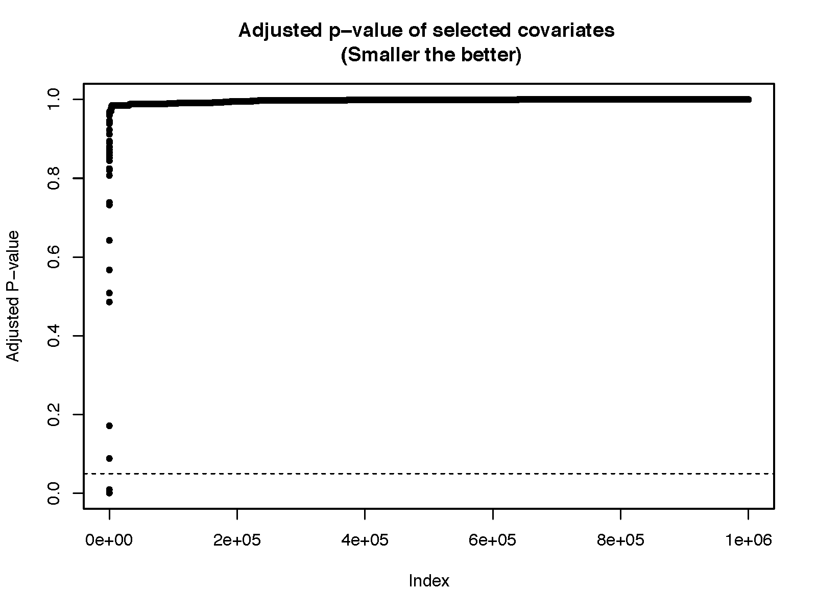
Figure 1: Plot of adjusted p-values using all response covariates

Running the data-adaptive algorithm on the parameter-generating samples provides a reasonable recovery of true effect responses. The results are given below:

Table 1: Summary of the results of data-adaptive statistical target parameter estimation

	covar. ID	ATE est.	p-value	adjusted p-value	mean CV-rank	% times in top 15
1	6	1.3474	2.05E-10	3.07E-09	1.1	100
2	1	1.2498	1.35E-08	9.72E-08	2.4	100
3	4	1.2406	1.94E-08	9.72E-08	2.8	100
4	5	1.0822	1.08E-07	4.04E-07	4.8	100
5	10	1.0250	3.43E-07	8.58E-07	7.3	90
6	16109	0.9605	3.32E-07	8.58E-07	11.4	70
7	8	0.9793	1.12E-05	1.38E-05	11.5	70
8	9	0.9073	3.11E-06	5.18E-06	26.9	40
9	23969	0.9172	2.66E-05	2.66E-05	27	50
10	910425	0.9107	2.07E-06	4.43E-06	27.1	30
11	398395	0.8975	7.44E-06	1.01E-05	27.7	20
12	975142	0.9127	2.94E-06	5.18E-06	28.1	40
13	963171	0.9124	1.19E-05	1.38E-05	28.7	40
14	491156	0.9425	5.36E-06	8.04E-06	31.7	50
15	619251	0.8970	1.55E-05	1.66E-05	35.2	50

From the table, it is clear that the approach of data-adaptive statistical target parameter estimation consistently picks out the true effects in the top candidates. After application of the Benjamini and Hochberg (1995) procedure on the reduced set of responses, $74$ out of $10$ true signals are still significant.

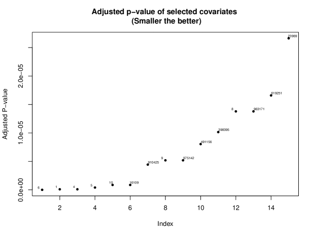
Figure 2: Plot of adjusted p-values using data-adaptive test statistics

4 Differentially expressed microRNA and exposure to benzene

Benzene, an established cause of acute myeloid leukemia (AML), may also cause one or more lymphoid malignancies in humans. Previous studies have identified single nucleotide polymorphisms (SNP) and patterns of DNA methylation associated with exposure to benzene through transcriptomic analyses of blood cells from a small number of occupationally exposed workers (Zhang et al., 2010); however, in these studies, the effect of benzene-induced changes to microRNA expression (Affymetrix 3.0 GeneChips which contain probes for $5639$ human miRNAs) in blood cells was not the subject of intense scrutiny. We discuss a study of 85 individuals in Tianjin, China, in which 56 workers exposed to varying levels of benzene and 29 unexposed control counterparts were monitored repeatedly for up to 12 months. For each individual, blood samples were collected and miRNA expression was measured and log-transformed, leading to the formulation of a statistical problem in which a large number of comparisons arises from performing miRNA screens on both exposed subjects and unexposed controls.

To illustrate the flexibility of the proposed method we will show how it can be used as a powerful test for differentially expressed microRNA. The data consist of 5639 real-valued outcomes and one binary treatment for 85 individuals. In univariate testing, the microRNA hsa-miR-320a_st has the smallest p-value ($p<0.000455$). However the association is no longer significant after controlling for multiple testing using the Benjamini-Hochberg (Benjamini and Hochberg, 1995) method to control the False Discovery Rate ($p_{adjusted}=0.5281$). Since our objective of interest was to detect the top differentially expressed microRNAs. (and not to differentiate all microRNAs), we generated data-adaptive test statistics to reduce the number of hypotheses based on the procedure outlined in 2.1

Table 2: Top microRNA’s after direct applying Benjamini-Hochberg (Down-regulated)

	microRNA	ATE	Fold Change	p-value	adjusted p-value
1	hsa-miR-744_st	-0.35	0.79	0.00067	0.52814
2	hsa-miR-320b_st	-0.32	0.80	0.00046	0.52814
3	hsa-miR-320a_st	-0.31	0.80	0.00045	0.52814
4	hsa-miR-320c_st	-0.30	0.81	0.00082	0.52814
5	hp_hsa-mir-449b_x_st	-0.23	0.85	0.00084	0.52814
6	ENSG00000238375_st	-0.20	0.87	0.00071	0.52814
7	hp_hsa-mir-4645_st	-0.18	0.88	0.00077	0.52814

Table 3: Top microRNA’s after direct applying Benjamini-Hochberg (Up-regulated)

	microRNA	ATE	Fold Change	p-value	adjusted p-value
1	hsa-miR-338-5p_st	0.83	1.78	0.00079	0.52814
2	hsa-miR-103a-2-star_st	0.66	1.58	0.00061	0.52814
3	hsa-miR-4725-3p_st	0.34	1.26	0.00094	0.53127

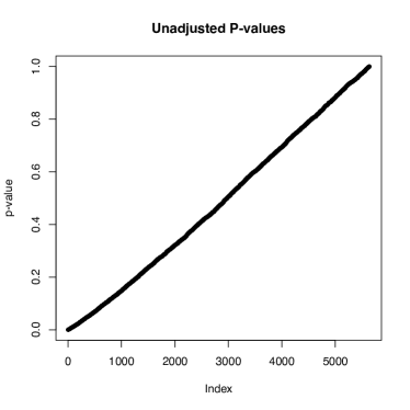
(a) (b)

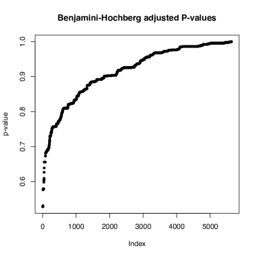
Figure 3: Plot of (a) unadjusted and (b) FDR adjusted p-values using all covariates

Given the multiplicity of comparisons, we propose the use of data-adaptive test statistics to reduce the number of comparisons first, thereby increasing power, while still maintaining accurate statistical inference. We specified the reduced set of response matrix $\widehat{Y}$ with dimension $n\times 30$, which correspond to studying top 30 microRNAs that will express differently under benzene exposure. We carried out 10-fold cross-validation to calculate the data-adaptive test statistics and tested each of the top 30 microRNAs. We finally performed FDR correction ((Benjamini and Hochberg, 1995)) on the 30 raw p-values.

4.1 Results

The results for the top 30 microRNAs and their FDR-adjusted p-values are shown in Table 4. 19 out of 30 top microRNAs had a significant differential expression (q-value $<0.05$) while we found none in FDR-corrected t-tests in Table 2. Observing the plot of FDR-adjusted p-values (Figure 4) also gives us insights as we can easily identify groups of significant p-values. In practice, we can choose a cutoff based on the trend of sorted p-values. The average rank of the top covariates (in Table 4) can also be referenced as a measure of stability of the effect across different subjects.

Table 4: Summary of the data-adaptive test statistics on miRNA data (Down-regulated)

	microRNA	ATE	raw p-values	adjusted p-values	avg rank	% appear in top 30
1	hsa-miR-134_st	-0.87	0.0197	0.0492	2.4	100
2	hsa-miR-3613-3p_st	-0.86	0.0003	0.0089	2.7	100
3	hsa-miR-4668-5p_st	-0.77	0.0034	0.0144	4.5	100
4	hsa-miR-382_st	-0.80	0.0294	0.0493	6.2	100
5	U49A_s_st	-0.70	0.0019	0.0114	7.5	100
6	hsa-miR-409-3p_st	-0.75	0.0312	0.0493	8.1	100
7	hsa-miR-3651_st	-0.67	0.0271	0.0493	8.7	100
8	hsa-miR-432_st	-0.72	0.0657	0.0777	10.0	100
9	hp_hsa-mir-548ai_st	-0.63	0.0169	0.0461	11.6	100
10	hsa-miR-1301_st	-0.61	0.0008	0.0114	11.7	100
11	hsa-miR-1275_st	-0.57	0.0015	0.0114	14.9	100
12	hsa-miR-200c_st	-0.57	0.0016	0.0114	16.2	90
13	ENSG00000199411_s_st	-0.56	0.0438	0.0597	16.7	80
14	hp_hsa-mir-548ai_x_st	-0.52	0.0229	0.0493	22.8	80
15	hsa-miR-423-5p_st	-0.50	0.0023	0.0117	23.6	80
16	U56_st	-0.51	0.0503	0.0656	24.5	80
17	ENSG00000252921_x_st	-0.49	0.0048	0.0180	26.9	70
18	U49B_s_st	-0.49	0.0112	0.0335	27.3	80
19	U38A_st	-0.49	0.0749	0.0833	28.4	70
20	hsa-miR-3613-5p_st	-0.51	0.2265	0.2343	30.5	70
21	hsa-miR-99b_st	-0.47	0.0674	0.0777	33.8	50
22	hsa-miR-486-5p_st	-0.46	0.0054	0.0181	34.5	70
23	hsa-miR-339-3p_st	-0.45	0.0245	0.0493	37.3	40
24	U49A_st	-0.43	0.0309	0.0493	39.7	30
25	HBII-85-2_x_st	-0.43	0.0247	0.0493	39.9	20
26	U21_st	-0.44	0.0391	0.0559	39.9	40
27	hsa-miR-4529-3p_st	-0.49	0.2706	0.2706	42.0	50
28	hsa-miR-940_st	-0.44	0.0340	0.0510	42.2	50
29	hsa-miR-584_st	-0.45	0.0796	0.0853	42.3	50
30	hsa-miR-150-star_st	-0.43	0.0524	0.0656	43.6	20

Table 5: List of microRNA’s that are still significant after FDR correction (Down-regulated)

	microRNA
1	hsa-miR-134_st
2	hsa-miR-3613-3p_st
3	hsa-miR-4668-5p_st
4	hsa-miR-382_st
5	U49A_s_st
6	hsa-miR-409-3p_st
7	hsa-miR-3651_st
8	hp_hsa-mir-548ai_st
9	hsa-miR-1301_st
10	hsa-miR-1275_st
11	hsa-miR-200c_st
12	hp_hsa-mir-548ai_x_st
13	hsa-miR-423-5p_st
14	ENSG00000252921_x_st
15	U49B_s_st
16	hsa-miR-486-5p_st
17	hsa-miR-339-3p_st
18	U49A_st
19	HBII-85-2_x_st

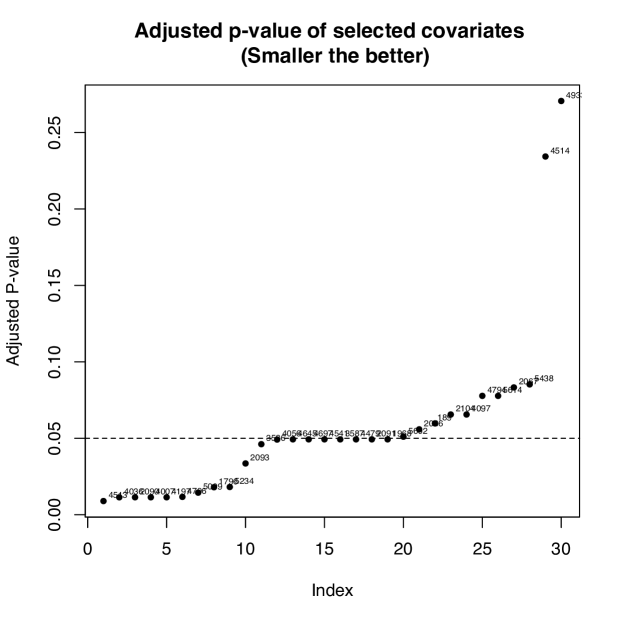
Figure 4: Adjusted p-values using data-adaptive test statistics (Down-regulated)

The same analysis can be performed on up-regulated microRNA’s. 20 out of 30 top microRNAs had a significant differential expression (q-value $<0.05$) as did the hsa-miR-338-5p_st and hsa-miR-103a-2-star_st that we found in FDR-corrected t-tests in Table 3.

Table 6: Summary of the data-adaptive test statistics on miRNA data (Up-regulated)

	microRNA	ATE	raw p-value	adjusted p-value	avg rank	% appear in top 30
1	hsa-miR-505_st	1.0175	0.001144	0.006465	1.2	100
2	hsa-miR-4772-3p_st	0.8763	0.001508	0.006465	3.4	100
3	hsa-miR-10a_st	0.8983	0.000979	0.006465	3.8	100
4	hsa-miR-338-5p_st	0.8313	0.000155	0.002986	5.3	100
5	hsa-miR-301a_st	0.8373	0.011351	0.026194	5.4	100
6	hsa-miR-212_st	0.8158	0.001421	0.006465	6.1	100
7	hsa-miR-374b_st	0.7728	0.035704	0.051006	7.6	100
8	hsa-miR-454_st	0.776	0.012762	0.02691	7.9	100
9	hsa-miR-7-1-star_st	0.7271	0.013911	0.02691	10.1	100
10	hsa-miR-4674_st	0.727	0.047842	0.064645	12.4	90
11	hsa-miR-30b_st	0.6837	0.094063	0.104514	14.3	100
12	hsa-miR-29c-star_st	0.6499	0.002409	0.009034	15.5	100
13	hsa-miR-103a-2-star_st	0.6597	0.000199	0.002986	15.8	100
14	hsa-let-7d-star_st	0.6519	0.014352	0.02691	16.4	100
15	hsa-miR-142-5p_st	0.6668	0.049561	0.064645	17.7	90
16	hsa-miR-361-3p_st	0.6136	0.02849	0.043226	20.5	90
17	hsa-miR-1231_st	0.6032	0.005194	0.01501	21.1	90
18	hsa-miR-99a_st	0.6099	0.119402	0.123519	22.4	80
19	hsa-miR-589-star_st	0.5867	0.018542	0.032722	23	80
20	hsa-miR-3188_st	0.581	0.001158	0.006465	24.3	80
21	hsa-miR-3621_st	0.5967	0.091534	0.104514	25	70
22	hsa-let-7g_st	0.5883	0.212763	0.212763	29.3	70
23	hsa-miR-148a_st	0.5586	0.113839	0.12197	29.3	60
24	hsa-miR-378g_st	0.537	0.021924	0.036541	32.1	40
25	hsa-miR-30e-star_st	0.5392	0.082371	0.098846	32.6	40
26	hsa-miR-641_st	0.531	0.005503	0.01501	33.3	30
27	hsa-miR-221-star_st	0.546	0.028817	0.043226	33.6	60
28	hsa-miR-181a-star_st	0.5398	0.057202	0.071502	34.1	60
29	hsa-miR-186_st	0.5304	0.009065	0.02266	34.5	30
30	hsa-miR-3187-3p_st	0.524	0.005102	0.01501	35.7	30

Table 7: List of microRNA’s that are still significant after FDR correction (Up-regulated)

	microRNA
1	hsa-miR-505_st
2	hsa-miR-4772-3p_st
3	hsa-miR-10a_st
4	hsa-miR-338-5p_st
5	hsa-miR-301a_st
6	hsa-miR-212_st
7	hsa-miR-454_st
8	hsa-miR-7-1-star_st
9	hsa-miR-29c-star_st
10	hsa-miR-103a-2-star_st
11	hsa-let-7d-star_st
12	hsa-miR-361-3p_st
13	hsa-miR-1231_st
14	hsa-miR-589-star_st
15	hsa-miR-3188_st
16	hsa-miR-378g_st
17	hsa-miR-641_st
18	hsa-miR-221-star_st
19	hsa-miR-186_st
20	hsa-miR-3187-3p_st

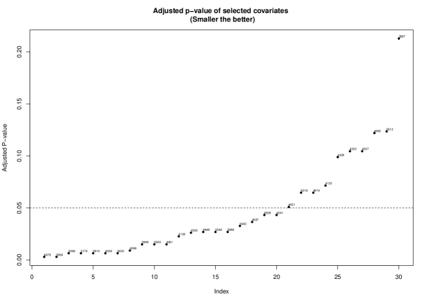
Figure 5: Adjusted p-values using data-adaptive test statistics (Up-regulated)

Overall, this formally confirms the conclusions in the paper that by generating the data-adaptive test statistics we can increase the power of testing a large set of statistical hypotheses and at the same time control the level of false positive rate (or false discovery rate).

5 Discussion

The goal of this article is to introduce a generalized class of robust procedures for performing statistical tests in high-dimensional settings, relying on the approach of data-adaptive statistical target parameters. Here, we have introduced, in generality, the theory and methodology underlying the use of data-adaptive statistics for multiple testing, illustrating key advantages of this approach via simulation studies and providing examples where relevant. By providing the theoretical formalisms in a generalized way, we have exposed a flexible framework in which the number of multiple testing corrections applied in high-dimensional problems can be reduced, allowing for signals that would otherwise be made undetectable by said corrections to be recovered.

In the example provided, we demonstrate the power of the approach based on data-adaptive test statistics in the context of a study of miRNA. We show that this new class of approaches for analyzing high-dimensional data sets allows researchers to derive improved statistical power in problems plagued by multiple testing, by allowing for relatively fewer null hypotheses of interest to be generated data-adaptively – that is, suggested by the observed data. In order to improve accessibilty to the methodology presented herein, Cai et al. (2017) have developed and made publicly available an open-source software package for data-adaptive multiple testing, available for the R statistical computing language (R Core Team (2016)).

References

- Benjamini and Hochberg (1995) Benjamini, Y., Hochberg, Y., 1995. Controlling the false discovery rate: a practical and powerful approach to multiple testing. Journal of the Royal Statistical Society. Series B (Methodological), 289–300.
- Cai et al. (2017) Cai, W., Hubbard, A. E., Hejazi, N. S., 2017. data.adapt.multi.test: Data-adaptive statistics for high-dimensional multiple testing. The Journal of Open Source Software (Submitted).
- Gerlovina and Hubbard (2016) Gerlovina, I., Hubbard, A. E., 2016. Big data, small sample: Peter Hall’s legacy – the Edgeworth expansion approach to inference. Submitted.
- Hubbard et al. (2016) Hubbard, A. E., Kherad-Pajouh, S., van der Laan, M. J., 2016. Statistical inference for data adaptive target parameters. The International Journal of Biostatistics 12 (1), 3–19.
- Hubbard and van der Laan (2016) Hubbard, A. E., van der Laan, M. J., 2016. Mining with inference: Data-adaptive target parameters. In: Buhlmann, P., Drineas, P., Kane, M., van der Laan, M. J. (Eds.), Handbook of Big Data. CRC Press, Taylor & Francis Group, LLC: Boca Raton, FL.
-
R Core Team (2016)
R Core Team, 2016. R: A Language and Environment for Statistical Computing. R
Foundation for Statistical Computing, Vienna, Austria.
URL https://www.R-project.org/ - van der Laan and Petersen (2012) van der Laan, M. J., Petersen, M. L., 2012. Targeted learning. In: Ensemble Machine Learning. Springer, pp. 117–156.
- Wienholds et al. (2005) Wienholds, E., Kloosterman, W. P., Miska, E., Alvarez-Saavedra, E., Berezikov, E., de Bruijn, E., Horvitz, H. R., Kauppinen, S., Plasterk, R. H., 2005. MicroRNA expression in zebrafish embryonic development. Science 309 (5732), 310–311.
- Wienholds and Plasterk (2005) Wienholds, E., Plasterk, R. H., 2005. MicroRNA function in animal development. FEBS letters 579 (26), 5911–5922.
- Zhang et al. (2010) Zhang, L., McHale, C. M., Rothman, N., Li, G., Ji, Z., Vermeulen, R., Hubbard, A. E., Ren, X., Shen, M., Rappaport, S. M., et al., 2010. Systems biology of human benzene exposure. Chemico-Biological Interactions 184 (1), 86–93.