Initial conditions for slow-roll inflation
in a random Gaussian landscape

Abstract

In the landscape perspective, our Universe begins with a quantum tunneling from an eternally-inflating parent vacuum, followed by a period of slow-roll inflation. We investigate the tunneling process and calculate the probability distribution for the initial conditions and for the number of e-folds of slow-roll inflation, modeling the landscape by a small-field one-dimensional random Gaussian potential. We find that such a landscape is fully consistent with observations, but the probability for future detection of spatial curvature is rather low, $P\sim 10^{-3}$.

1 Introduction

String theory predicts the existence of a vast landscape of vacuum states with diverse properties Susskind:2003kw ; BoussoPolchinski . In the cosmological context this leads to the picture of an eternally inflating multiverse, where different spacetime regions are occupied by different vacua. Transitions between the vacua occur through quantum tunneling, with bubbles of daughter vacuum nucleating and expanding in the parent vacuum background. According to this picture, our local region originated as a result of tunneling from some inflating parent vacuum and then went through a period of slow-roll inflation. The number of vacua in the landscape is expected to be enormous, so predictions in this kind of model must necessarily be statistical. The properties of string theory landscape are not well understood, and the approach adopted in much of the recent work is to substitute it by a scalar field model with a random Gaussian potential Tegmark ; Easther ; Frazer ; Battefeld ; McAllister:2012am ; Yang:2012jf ; Pedro:2013nda ; Marsh:2013qca ; Bachlechner ; Wang ; MV ; Freivogel:2016kxc ; Pedro:2016sli ; EastherGuthMasoumi .

In a recent paper MVY we developed analytic and numerical techniques for studying the statistics of slow-roll inflation in random Gaussian landscapes. We applied these techniques to the simplest case of small-field inflation in a one-dimensional random landscape. In this case, inflation typically occurs at local maxima or at inflection points of the potential LindeWestphal . Focusing mostly on the inflection points, we found the probability distributions for the maximal number of inflationary e-folds $N_{\rm max}$ and for the spectral index of density fluctuations $n_{s}$.

The maximal e-fold number $N_{\rm max}$ depends only on the shape of the potential near the inflection point, but the actual number of e-folds, $N_{e}$, is sensitive to the initial conditions – that is, to the initial value $\phi_{0}$ of the inflaton field right after it tunnels from the parent vacuum. If $\phi_{0}$ is too far away from the inflection point, the field may develop a large velocity and overshoot or it may miss the slow-roll region entirely. In the present paper we shall use numerical simulations to determine the probability distribution for $\phi_{0}$ and to investigate its effect on the statistical properties of inflation. As before, we shall restrict our analysis to the simplest case of one-dimensional potentials.

In the next Section we review some general properties of random Gaussian potentials, and in Sec. 3 we summarize earlier work on inflection-point inflation. Our numerical simulations and the results for the distribution of $\phi_{0}$ are presented in Sec. 4. In Sec. 5 we develop a semi-analytic method to study the evolution of the scalar field after tunneling. We find the probability distribution for the number of e-folds of slow-roll inflation $N_{e}$ and discuss the implications of our results for the prospects of detection of spatial curvature. Our conclusions are summarized and discussed in Sec. 6. Some technical details related to the simulations are relegated to the appendices. Throughout the paper we use reduced Planck units with $8\pi G=1$.

2 Random Gaussian landscapes

Consider a one-dimensional random Gaussian landscape model with a potential $U(\phi)$ satisfying the following correlation function:

$$\langle U(\phi_{1})U(\phi_{2})\rangle=F(|\phi_{1}-\phi_{2}|)=\frac{1}{2\pi}\int{\rm d}{k}\,P(k)e^{i{k}(\phi_{1}-\phi_{2})}~{}.$$ (1)

We specifically consider a Gaussian-type correlation function defined as

$$F(\phi)=U_{0}^{2}e^{-\phi^{2}/2\Lambda^{2}},$$ (2)

with $\Lambda$ playing the role of the correlation length in the landscape. Then the spectral function $P(k)$ is given by

$$P(k)=U_{0}^{2}(2\pi\Lambda^{2})^{1/2}e^{-\Lambda^{2}k^{2}/2}.$$ (3)

We define different moments of the spectral function as

$$\sigma_{n}^{2}=\frac{1}{2\pi}\int dk(k^{2})^{n}P(k)=\frac{2^{n}\Gamma\left(n+\frac{1}{2}\right)}{\Gamma\left(\frac{1}{2}\right)}\frac{U_{0}^{2}}{\Lambda^{2n}},$$ (4)

where we used Eq. (3) in the second line.

Once we specify a set of points $\{\phi_{1},\ldots,\phi_{n}\}$ and define $U_{j}\equiv U(\phi_{j})$, the probability distribution for $U_{j}$ is given by

$$P(U)=\frac{\sqrt{{\rm det}M^{-1}_{ij}}}{(2\pi)^{n/2}}e^{-\frac{1}{2}U_{i}M^{-1}_{ij}U_{j}}~{},$$ (5)

where the positive definite matrix $M$ is an $n\times n$ matrix of correlators defined by

$$M_{ij}\equiv F\left(|\phi_{i}-\phi_{j}|\right)~{}.$$ (6)

Since $M_{ij}$ is a symmetric matrix, we can diagonalize it by an orthogonal matrix $\cal O$. Then the probability distribution for variables $\beta_{i}\equiv{\cal O}_{ij}U_{j}$ is given by

$$P(\beta)=\frac{\sqrt{\prod_{i}\lambda_{i}}}{(2\pi)^{n/2}}e^{-\frac{1}{2}\lambda_{i}\beta_{i}^{2}}~{},$$ (7)

where $\lambda_{i}$’s are eigenvalues of the matrix $M_{ij}$. Such random variables can be easily generated in numerical simulations.

When the values of $U(\phi_{j})$ are generated at a sufficient density on the $\phi$-axis, we can interpolate them to obtain a smooth potential. We check in the App. A that this procedure typically saturates at a few points per correlation length $\Lambda$: the interpolated potential changes very little with the addition of more points. We shall use this method with four points per correlation length to generate realizations of a random Gaussian landscape.

Assuming that our universe is a result of a bubble nucleation event, we anticipate that the state of the universe after nucleation allows for a prolonged period of inflation. This is possible for parts of the landscape that resemble Fig. 1, which includes a parent vacuum and a daughter vacuum separated by a barrier. We shall refer to parent and daughter vacua as “false” (FV) and “true” (TV) vacua, respectively. The inflection points where $U^{\prime\prime}=0$ are marked by red dots in the figure. In this example, there are three inflection points between the top of the barrier and the true vacuum. The potential is rather flat near the middle inflection point ($U^{\prime}$ and $U^{\prime\prime}$ are small), and slow-roll inflation can be expected to occur in this region.

We are going to focus on the case when the correlation length of the potential is small compared to the Planck scale, $\Lambda\ll 1$. Inflation in this case is typically of the small-field type: the slow-roll occurs in a narrow range $\Delta\phi\ll\Lambda$ and the potential during the slow-roll remains approximately constant.

The correlation function (2) implies that the average value of the potential is $\langle U(\phi)\rangle=0$, so positive and negative values of $U(\phi)$ are equally likely. In this case, the minima of the potential are predominantly at negative values of $U$. This effect is especially pronounced for higher-dimensional random landscapes, where positive-energy vacua may not exist at all BrayDean ; Battefeld . This problem can be alleviated by adding a constant shift term to the potential, $U(\phi)\to U(\phi)+C$. One can also consider models where $C$ is variable, but its characteristic scale of variation is much greater than $\Lambda$. For example, in axionic landscapes this term can have the form $C(\phi)=m^{2}\phi^{2}/2$ with a very small mass $m$ MV or $C(\phi)\propto\cos(\mu\phi)$ with $\mu\ll 1/\Lambda$ evil . Then the local properties of the potential are still determined by the correlator (2), while the extra term provides an additive shift, which is characterized by its own probability distribution.

Here, we are interested in the case when the true vacuum has an almost vanishing vacuum energy. In a generic landscape, the number of such vacua is extremely small, and trying to find them by random sampling is a hopeless task. In our numerical simulations we simply added a constant to the generated random potential, so that $U=0$ in the true vacuum. We expect the resulting ensemble of realizations to be similar to what one would get by random sampling in a landscape with a flat distribution of the shift parameter $C$.

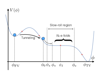
Figure 1: A schematic picture of the kind of potential we are interested in. Inflection points are marked by red dots.

3 Analytic results for inflection-point inflation

Inflection-point inflation was first studied by Baumann et al Baumann . Here we review some of their results, which will be useful in subsequent sections.

The necessary conditions for slow-roll inflation are $\epsilon_{s},\eta_{s}\ll 1$, where

$$\epsilon_{s}=\frac{1}{2}\left(\frac{U^{\prime}}{U}\right)^{2},$$ (8)

$$\eta_{s}=\frac{U^{\prime\prime}}{U}.$$ (9)

Note that the values of the slow-roll parameters at a randomly chosen point in the landscape are typically given by $\epsilon_{s}\sim\eta_{s}\sim\Lambda^{-2}\gg 1$, so inflation can occur only in rare regions of the landscape.

To study inflection-point inflation, we approximate the potential by a third-order Taylor expansion,

$$U(\phi)=U_{\rm I}+{U_{\rm I}}^{\prime}\phi+\frac{1}{3!}{U_{\rm I}}^{\prime\prime\prime}\phi^{3},$$ (10)

where the subscript $I$ indicates the value at the inflection point $\phi_{\rm I}$, which is set to be at $\phi_{\rm I}=0$: ${U_{\rm I}}^{\prime\prime}=0$. The slow-roll conditions require that ${U_{\rm I}}^{\prime}\ll U_{\rm I}$, but ${U_{\rm I}}^{\prime\prime\prime}$ does not need to be small, and we shall assume it to be comparable to the rms value, ${U_{\rm I}}^{\prime\prime\prime}\sim U_{0}/\Lambda^{3}$. The slow-roll region is then determined mainly by the condition $\eta_{s}\ll 1$ and can be specified as $[\phi_{s},\phi_{e}]$, where

$$\phi_{s}\sim-\frac{U_{\rm I}}{\lvert{U_{\rm I}}^{\prime\prime\prime}\rvert},$$ (11)

$$\phi_{e}\sim\frac{U_{\rm I}}{\lvert{U_{\rm I}}^{\prime\prime\prime}\rvert}.$$ (12)

We assume that ${U_{\rm I}}^{\prime}{U_{\rm I}}^{\prime\prime\prime}>0$, since otherwise the potential has a shallow high-energy minimum near the inflection point and inflation drives the field into that minimum MVY .

It follows from (11),(12) that the size of the slow-roll region is typically $\Delta\phi\sim\Lambda^{3}\ll\Lambda$. This justifies the assumption that $U(\phi)$ can be approximated by a constant in this region.

The “maximal e-folding number” can be defined as

$$N_{\rm max}=-\int_{\phi_{s}}^{\phi_{e}}d\phi\frac{U(\phi)}{U^{\prime}(\phi)}\approx-\int_{-\infty}^{\infty}d\phi\frac{U(\phi)}{U^{\prime}(\phi)}\approx\pi\sqrt{2}\frac{U_{\rm I}}{\sqrt{{U_{\rm I}}^{\prime}{U_{\rm I}}^{\prime\prime\prime}}},$$ (13)

where we have assumed that $N_{\rm max}\gg 1$ (which is necessary for extending the integration to $\pm\infty$).

The spectral index $n_{s}$ can be expressed in terms of $N_{\rm max}$ as

$$n_{s}\simeq 1-\frac{4\pi}{N_{\rm max}}{\rm cot}\left(\frac{\pi N_{e}^{(\rm CMB)}}{N_{\rm max}}\right),$$ (14)

where $N_{e}^{(\rm CMB)}$ ($\simeq 50$-$60$) is the e-folding number at which the CMB scale leaves the horizon. It follows from (14) that $n_{s}$ is greater than $1-4/N_{e}^{(\rm CMB)}\approx 0.92$, which is approached in the limit $N_{\rm max}\to\infty$. Note that for hilltop inflation $n_{s}<0.92$ MVY , while the observed value is $n_{s}\approx 0.97$ and lies in the inflection-point range. This provides additional motivation to focus our analysis on inflection-point inflation.

The magnitude of density fluctuations is given by

$$\Delta_{R}^{2}=\frac{1}{12\pi}\frac{U_{\rm I}^{3}}{{{U_{\rm I}}^{\prime}}^{2}}=\frac{N_{\rm max}^{4}}{48\pi^{6}}\frac{{{U_{\rm I}}^{\prime\prime\prime}}^{2}}{U_{\rm I}}\sim\frac{U_{0}N_{\rm max}^{4}}{48\pi^{6}\Lambda^{6}},$$ (15)

where in the second step we used Eq. (13) for $N_{\rm max}$ and in the last step we assumed that $U_{\rm I}$ and ${U_{\rm I}}^{\prime\prime\prime}$ have their typical values. The observed value of $\Delta_{R}^{2}\sim 4\times 10^{-9}$ can be obtained by adjusting the parameters $U_{0}$ and $\Lambda$:

$$\frac{U_{0}}{\Lambda^{6}}\sim 10^{-12}\left(\frac{100}{N_{\rm max}}\right)^{4}\lesssim 10^{-12}.$$ (16)

The probability distributions for $N_{\rm max}$ and $n_{s}$ in a random Gaussian landscape have been calculated in Ref. MVY . Here we quote the results:

$$P(N_{\rm max})\propto N_{\rm max}^{-3},$$ (17)

$$P(n_{s})=P(N_{\rm max})\frac{{\rm d}N_{\rm max}}{{\rm d}n_{s}}.$$ (18)

The distribution (17) gives the probability that a randomly chosen inflection point in the landscape is characterized by a given value of $N_{\rm max}$. Note, however, that here we are interested only in inflection points located between a high-energy false vacuum and a zero-energy true vacuum, as shown in Fig. 1. As explained in Sec. 2, we obtain such configurations by adding a constant term to a randomly generated potential. This procedure changes the value of $U$ at the inflection point; hence it affects the value of $N_{\rm max}$ in Eq. (13) and may potentially affect the distribution (17). We shall see, however, that the form of this distribution remains unchanged.

As we mentioned in the Introduction, the actual number of inflationary e-folds $N_{e}$ depends on the initial conditions after tunneling and is generally different from $N_{\rm max}$. We shall find the probability distributions for the initial conditions and for $N_{e}$ in the following sections.

4 Initial conditions for inflation

4.1 General formalism

Decay of the false vacuum occurs through bubble nucleation, which is a quantum tunneling process. In the semiclassical approximation, the tunneling is described by an $O(4)$-symmetric instanton $\phi(r)$, which can be found by solving the Euclidean field equation Coleman

$$\frac{d^{2}\phi}{dr^{2}}+\frac{3}{r}\frac{d\phi}{dr}=\frac{dU}{d\phi}~{}.$$ (19)

Here we assume that gravitational effects on the tunneling can be neglected, which is usually the case in a small-field landscape. The boundary conditions for $\phi(r)$ are $\phi^{\prime}(r=0)=0$ and $\phi(r\to\infty)=\phi_{\rm FV}$, where $\phi_{\rm FV}$ is the value of $\phi$ in the false vacuum. The tunneling probability is determined mostly by the exponential factor,

$$P_{\rm tunneling}\propto e^{-S_{E}},$$ (20)

where $S_{E}$ is the Euclidean instanton action

$$S_{E}=\int_{0}^{\infty}{\rm d}r2\pi^{2}r^{3}\left(\frac{1}{2}\phi^{\prime 2}+U(\phi(r))-U_{\rm FV}\right),$$ (21)

and $U_{\rm FV}\equiv U(\phi_{\rm FV})$.

It will be convenient to introduce dimensionless variables ${\bar{\phi}}$ and ${\bar{r}}$ as

$$\phi=\Lambda{\bar{\phi}},$$ (22)

$$r=\Lambda U_{0}^{-1/2}{\bar{r}},$$ (23)

$$U(\phi)=U_{0}{\bar{U}}({\bar{\phi}}).$$ (24)

In terms of the new variables, Eq. (19) still has the same form,

$$\frac{d^{2}{\bar{\phi}}}{d{\bar{r}}^{2}}+\frac{3}{\bar{r}}\frac{d\bar{\phi}}{d{\bar{r}}}=\frac{d{\bar{U}}}{d{\bar{\phi}}}~{},$$ (25)

where the potential ${\bar{U}}({\bar{\phi}})$ is now characterized by the correlation function (2) with $U_{0}=\Lambda=1$. We note that

$$N_{\rm max}=\Lambda^{2}{\bar{N}}_{\rm max},$$ (26)

where ${\bar{N}}_{\rm max}$ is the maximal e-folding number for the rescaled potential ${\bar{U}}({\bar{\phi}})$. We also define the action $\bar{S}$ for the rescaled variables:

$$S_{E}=\frac{\Lambda^{4}}{U_{0}}\bar{S}.$$ (27)

The initial value $\phi_{0}$ of the inflaton field after tunneling is set by the value of ${\bar{\phi}}$ at the center of the instanton,

$$\phi_{0}=\Lambda{\bar{\phi}}(0).$$ (28)

The probability distribution for ${\phi}_{0}$ can now be found with the aid of numerical simulations.

It is well known that instanton solutions for multi-dimensional field spaces are not unique, because there may be more than one saddle point between the true vacuum and false vacuum. As we explain in App. B, there may also be multiple instanton solutions in the one-dimensional case, but for a different reason. For a generic potential, there is typically a single instanton describing tunneling to a close vicinity of the true vacuum. In the presence of a flat inflection region, additional instantons may appear, corresponding to tunneling to the neighborhood of the inflection point $\phi_{\rm I}$. As we make the inflection region flatter, at some point the instanton tunneling to the true vacuum disappears, and only tunneling to the vicinity of inflection point remains possible.

The number and character of the instantons also depend on the shape and height of the potential barrier. As an illustration we show some examples in Fig. 2, where the tunneling points $\phi_{0}$ are indicated by blue squares. All four potentials in the figure are rather similar, except they have different values of the false vacuum energy density $U_{\rm FV}$. In the upper left frame, $U_{\rm FV}$ is almost degenerate with $U_{\rm I}$ and there is a single instanton solution, which brings $\phi$ almost all the way to the true vacuum. In the upper right frame, $U_{\rm FV}$ is somewhat higher and additional instantons appear, which describe tunneling with $\phi_{0}$ close to the inflection point. As we explain in App. B, additional instanton solutions appear in pairs. As $U_{\rm FV}$ gets higher, the middle tunneling point moves towards the true vacuum tunneling point, and eventually the two points “annihilate”. In the lower right frame, $U_{\rm FV}$ is still higher, and tunneling is now possible only to the neighborhood of the inflection point.

When several instantons are present, one can compare the instanton actions to determine the dominant decay channel. We found that tunneling to the true vacuum dominates in most of these cases. We note, however, that in the present context we are interested in tunnelings that lead to sufficiently long inflation, regardless of their relative rate compared to other tunneling processes.

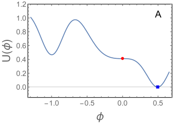
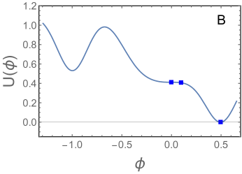
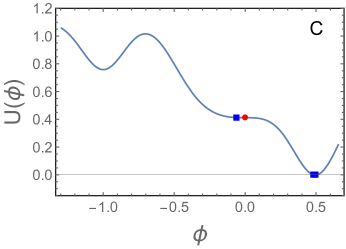
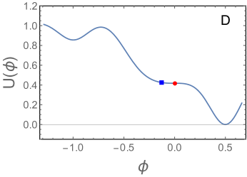
Figure 2: Tunneling points, represented by blue squares, are shown for potentials having similar shapes but different values of $U_{\rm FV}$. The relevant inflection points are marked by red dots. The upper left figure has a single tunneling to the true vacuum, the upper right and lower left figures have tunneling points to neighborhoods of both $\phi_{\rm TV}$ and $\phi_{\rm I}$. The bottom right potential has tunneling only to the neighborhood of $\phi_{\rm I}$.

To illustrate the dependence of the action of different instantons on the shape of the potential, we fix the potential on the right side of the barrier in Fig.2 and calculate the instanton actions for different values of $U_{\rm FV}$. The result is shown in Fig. 3. The red dashed (green solid) line is the action of the instanton solution that brings $\phi$ close to the true vacuum (inflection point). The blue dotted line is the one with $\phi_{0}$ between the other two tunneling points. We see that tunneling to the true vacuum dominates in (almost) the entire range where the corresponding instanton exists. The blue dotted line is always just above the green solid line; they are so close that they appear to coincide in the left frame of the figure. When $U_{\rm FV}$ increases to a certain threshold, the blue dotted line meets and annihilates with the red dashed line (see the right frame). Before the annihilation, the red dashed line crosses the green solid line, which means that tunneling to the inflection point becomes dominant. However, the region where this occurs is so small that we cannot see it in the left frame. Since the instanton solution with $\phi_{0}$ between the other two tunneling points is always subdominant, we neglect it in the rest of the paper. We denote the instanton action for solutions that bring $\phi$ close to the true vacuum (inflection point) as $S_{\rm T}$ ($S_{\rm I}$).

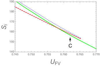
Figure 3: Action of different instanton solutions as a function of $U_{\rm FV}$ with other features of potential fixed, as explained in the text.

4.2 Numerical simulation

We used the procedure outlined in Sec. 2 to generate $2.0\times 10^{9}$ segments of a random Gaussian landscape, with each segment having length $8\Lambda$. The number of local minima in such a segment is almost always greater than or equal to two. We set the number of points per correlation length at $4$, which means that every segment contains 33 points $\phi_{j}$. We generate the values of the potential $U(\phi_{j})$ at these points according to the probability distribution (5) and use a fifth order spline to interpolate between them.

In each realization of $U(\phi)$, we identify all extrema and inflection points. For any pair of adjacent minima, we refer to the higher- and lower-energy ones as $\phi_{\rm FV}$ and $\phi_{\rm TV}$, respectively, and shift the potential so that $U_{\rm TV}=0$. We keep only realizations that have an inflection point $\phi_{\rm I}$ satisfying the following criteria: (i) it is located between the top of the barrier and the true vacuum, (ii) its energy density is lower than that of the false vacuum, $U_{\rm I}<U_{FV}$. This procedure is illustrated in Fig. 4.

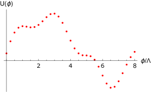
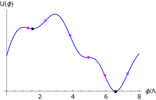
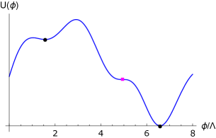
Figure 4: The procedure for choosing the relevant inflection and tunneling points as explained in the text. Potential values generated by the random Gaussian algorithm (upper left frame) are interpolated by a smooth curve (upper right frame). In the lower left frame the minima and the inflection points are marked by blue dots and magenta squares, respectively, and the potential is shifted so that $U_{\rm TV}=0$. The lower right frame shows the inflection point satisfying the selection criteria.

For each of the selected pairs of vacua, we seek instanton solutions of Eq. (25) using the shooting method. We then use Eq. (28) to find the initial value(s) of the field $\phi$ after tunneling.

4.3 Distributions for $\phi_{0}$ and $N_{\rm max}$

We plotted the distribution of the initial values ${\bar{\phi}}_{0}=\phi_{0}/\Lambda$ in the left panel of Fig. 5. Here and hereafter, the normalization of probability distributions is arbitrary. In cases where the potential admitted two instanton solutions, we included the values of $\bar{\phi}_{0}$ for both of them (disregarding the subdominant “middle” instanton). The distribution has a sharp peak centered near ${\bar{\phi}}_{0}=-0.1$ and a somewhat larger and broader peak at ${\bar{\phi}}_{0}\sim 1.3$. These peaks correspond to tunnelings to the vicinity of the inflection point $\bar{\phi}_{\rm I}=0$ and of the true vacuum $\bar{\phi}_{TV}$, respectively. In the right panel of Fig. 5 we plotted the distribution of ${\bar{\phi}}_{0}$ for tunnelings to the inflection point – that is, including only cases where $\bar{\phi}_{0}$ is closer to $\bar{\phi}_{\rm I}=0$ than to $\bar{\phi}_{TV}$. This distribution is peaked near ${\bar{\phi}}\approx-0.1$ with a width $\Delta{\bar{\phi}}\approx 0.4$.

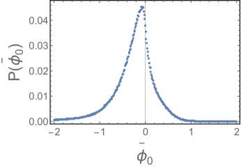
Figure 5: Histogram of $\bar{\phi}_{0}$ for all tunneling processes (left panel) and for the tunnelings to the inflection point (right panel).

Fig. 6 shows a histogram of the maximal e-fold number $\bar{N}_{\rm max}$, evaluated from Eq. (13). The result is well fitted by the analytic function

$$P(\bar{N}_{\rm max})\propto\bar{N}_{\rm max}^{-3},$$ (29)

which is shown by a red line in the figure. This shows that the form of the $\bar{N}_{\rm max}$ distribution is not affected by the shift of the potential to $U_{\rm TV}=0$.

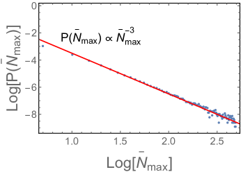
Figure 6: Histogram of $\bar{N}_{\rm max}$ for all eligible inflection points. The red line is an analytic function proportional to $\bar{N}_{\rm max}^{-3}$.

The plot in the left panel of Fig. 7 is the same as in Fig. 6, but now the contributions due to different types of instantons are shown separately. The green (magenta) lines represent the cases where there is only one instanton solution and $\bar{\phi}_{0}$ is closer to the inflection point (true vacuum). The red (blue) lines are for realizations with multiple instantons, where the dominant tunneling is to the inflection point (true vacuum). The type of instanton is not relevant for the present paper, but our results may be useful in other contexts, so we present them here for completeness. The figure shows that in the multiple instanton case the dominant tunneling channel is almost always to the true vacuum: the number of realizations with $S_{\rm I}<S_{\rm T}$ is suppressed by more than an order of magnitude. This is consistent with the discussion of the tunneling action in Sec. 4.1. We note also that the numbers of landscape realizations represented by blue and green curves are nearly the same and are within about a factor of 2 from those represented by the magenta curve. We have not found any explanation for this surprising fact. It implies that realizations with large values of $N_{\rm max}$ split into three comparable groups: a group with tunneling only to inflection point, a group with tunneling to the true vacuum, and a group with multiple tunneling channels, where the tunneling to the true vacuum dominates.

The right panel of Fig. 7 is a scatter plot of realizations in $\bar{\phi}_{0}$-$\bar{N}_{\rm max}$ plane, with the same color code as in the left panel. The average values $\langle\bar{\phi}_{0}\rangle$ are shown as yellow, magenta, and cyan lines for the data indicated by green, red, and blue dots, respectively. We see that $\langle\bar{\phi}_{0}\rangle$ is almost constant at $\bar{N}_{\rm max}\gg 1$ for all types of instantons, with $\langle\bar{\phi}_{0}\rangle\sim-0.4$ for the single instanton case and $\langle\bar{\phi}_{0}\rangle\sim-0.1$ for the multi-instanton case. This indicates that ${\bar{N}}_{\rm max}$ and ${\bar{\phi}}_{0}$ are essentially uncorrelated in the most interesting regime of large ${\bar{N}}_{\rm max}$.

From now on, we shall not distinguish between single and multi-instanton tunnelings and treat all inflection-point tunnelings on equal footing. In multi-instanton realizations with a dominant true-vacuum instanton, we keep only the inflection-point instanton. The reason is that true-vacuum tunneling is irrelevant for our discussion, and the tunneling processes described by inflection-point instantons occur regardless of whether or not there is a more probable tunneling channel.

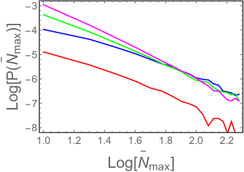
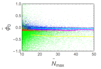
Figure 7: The left panel shows the distribution of $\bar{N}_{\rm max}$ for the single instanton case with tunneling to the inflection point (green) and to the true vacuum (magenta) and for the multiple instanton case with $\bar{S}_{\rm T}>\bar{S}_{\rm I}$ (red) and $\bar{S}_{\rm T}<\bar{S}_{\rm I}$ (blue). The right panel is a scatter plot in the ${\bar{N}}_{\rm max}-\phi_{0}$ plane with the same color code. The yellow, magenta, and cyan lines represent the averaged values of $\bar{\phi}_{0}$.

4.4 Tunneling action

The distributions for $\phi_{0}$ and $N_{\rm max}$ that we calculated here are defined as frequencies of occurrence in the landscape. They should not be confused with the probabilities of occurrence in the multiverse, which can be directly related to observational predictions. The problem of defining these probabilities is known as the measure problem, which at present remains unresolved. (For a review of the measure problem see Freivogel .) A number of different measure prescriptions have been suggested in the literature. Some of them lead to paradoxes or to a glaring conflict with observations and have therefore been ruled out. This process of elimination has not been enough to fix a unique measure of the multiverse. However, the measure prescriptions which are not obviously problematic tend to give similar predictions and introduce similar weighting factors for different realizations of the potential. The scale factor measure scalefactor1 ; scalefactor2 can be taken as a representative example of such “acceptable” measures.

For a given measure prescription, probabilities can be calculated by solving the rate equation, which is similar to the Boltzmann equation in the multiverse. Naively, one might expect that different tunneling realizations in the landscape should be weighted by the tunneling rate, which is proportional to $\exp(-S_{E})$, where $S_{E}$ is the tunneling action. However, analysis of the rate equation in the scale-factor measure shows that this expectation is incorrect. A simple counter-example is a landscape with an everywhere positive potential, $U(\phi)>0$. It can be shown that in such a landscape the probabilities depend only on the vacuum energy density and are independent of the transition rates Vanchurin . In general, the probability of a given vacuum has a complicated dependence on the transition rates between different vacua in the landscape, not just on the rate of tunneling to this particular vacuum. One also finds that transitions with a small tunneling action are not generally “rewarded” with a high weighting factor. The reason can be roughly explained as follows. The weighting factor for vacuum $i$ due to tunneling from a false vacuum $j$ is proportional to $\kappa_{ij}f_{j}$, where $\kappa_{ij}$ is the tunneling rate from $j$ to $i$ per Hubble volume per Hubble time, and $f_{j}$ is the volume fraction occupied by vacuum $j$ on constant scale factor surfaces. If the tunneling rate is very high, this leads to a rapid depletion of the false vacuum, so $f_{j}$ gets very small. These two effects tend to compensate one another. On the other hand, tunnelings with a large instanton action tend to be disfavored in the presence of other decay channels with a smaller action.

A study of the rate equation in a random Gaussian landscape would require a complicated statistical analysis, which is beyond the scope of the present paper. To facilitate such analysis in future work, here we shall analyze possible correlations of the action ${\bar{S}}$ with ${\bar{\phi}}_{0}$ and ${\bar{N}}_{\rm max}$. If present, such correlations may affect probabilities for the initial conditions and for the observational effects of inflation.

We show a scatter plot of ${\rm Log}[\bar{S}]$ and ${\rm Log}[\bar{N}_{\rm max}]$ in the left panel of Fig. 8. This includes only tunnelings to the inflection point. For large values of $\bar{N}_{\rm max}$, the rescaled instanton action is mostly in the range $100\lesssim{\bar{S}}\lesssim 10^{4}$. Note that the full action (27) is much larger than that. From Eq. (16) we have

$$\frac{\Lambda^{4}}{U_{0}}\gg 10^{12},$$ (30)

and thus $S_{E}\gg 10^{14}$. The plot suggests that for $\bar{N}_{\rm max}\gg 1$, $\bar{S}$ is essentially uncorrelated with $\bar{N}_{\rm max}$. In particular, the average value of ${\rm Log}[\bar{S}]$ is nearly constant at large $\bar{N}_{\rm max}$. This is not surprising, since the instanton action depends on the shape of the potential around the top of the barrier, while ${\bar{N}}_{\rm max}$ is not sensitive to this shape. The right panel of Fig. 8 shows the probability distribution of $\bar{N}_{\rm max}$ under the condition of $\bar{S}<100$. The distribution is still well fitted by $N_{\rm max}^{-3}$.

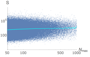
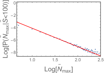
Figure 8: Scatter plot of ${\rm Log}[\bar{S}]$ and ${\rm Log}[\bar{N}_{\rm max}]$ (left panel) and the probability distribution of ${\rm Log}[\bar{N}_{\rm max}]$ under the condition of $\bar{S}<100$ (right panel). The left panel also shows the average value of $\bar{S}$ as a function of ${\bar{N}}_{\rm max}$, and the right panel shows the function ${\bar{N}}_{\rm max}^{-3}$.

Figure 9 is a scatter plot in the ${\rm Log}[\bar{S}]$-${\rm Log}[-\bar{\phi}_{0}]$ plane for $\bar{N}_{\rm max}>30$. It exhibits significant correlation between $\bar{S}$ and $\bar{\phi}_{0}$. In particular, the number of realizations with large values of ${\bar{S}}$ increases towards small values of $\bar{\phi}_{0}$. This can be understood as the contribution of realizations with $U_{\rm FV}\approx U_{\rm I}$, which correspond to the thin-wall regime. In the limit $U_{\rm FV}\to U_{\rm I}$, the tunneling action diverges and $\bar{\phi}_{0}\to 0$ Coleman . On the other hand, the average value of S appears to saturate at a constant $\langle{\bar{S}}\rangle\sim 10^{5}$ at ${\bar{\phi}}\to 0$. In the rest of the paper we shall assume that the correlations between ${\bar{S}}$ and ${\bar{\phi}}_{0}$ have no significant effect on the probability distribution for $\phi_{0}$. This issue, however, requires some further study.

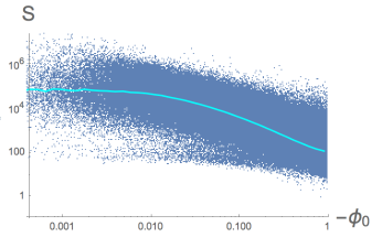
Figure 9: Scatter plot of ${\rm Log}[\bar{S}]$ and ${\rm Log}[-\bar{\phi}_{0}]$ under the condition of $\bar{N}_{\rm max}>30$.

5 Slow-roll inflation after tunneling

After tunneling, the bubble has the interior geometry of an open FRW universe,

$$ds^{2}=dt^{2}-a^{2}(t)\left(d\chi^{2}+\sinh^{2}\chi d\Omega^{2}\right).$$ (31)

Its evolution is described by the equations

$$\frac{{\dot{a}}^{2}}{a^{2}}=\frac{1}{3}\left(U(\phi)+\frac{{\dot{\phi}}^{2}}{2}\right)+\frac{1}{a^{2}},$$ (32)

$${\ddot{\phi}}+3\frac{\dot{a}}{a}{\dot{\phi}}+U^{\prime}(\phi)=0,$$ (33)

with the initial conditions at $t=0$

$${\dot{a}}(0)=1,~{}~{}~{}\phi(0)=\phi_{0},~{}~{}~{}{\dot{\phi}}(0)=0,$$ (34)

where $\phi_{0}$ is determined from the instanton solution. Our aim in this section is to find the probability distribution for the e-folding number after tunneling $N_{e}$.

We first note that the results of Sec. 4 for the initial value ${\bar{\phi}}_{0}=\phi_{0}/\Lambda$ are independent of $\Lambda$ and can be applied for any value of $\Lambda\ll 1$. Thus we expect the tunneling to occur to a point $\phi_{0}$ with a probability distribution of width

$$\Delta\phi_{0}\sim 0.4\Lambda,$$ (35)

near the inflection point (which we assume to be at $\phi=0$). We note also that the range of $\phi$ around the inflection point where slow-roll inflation is possible, $|\phi|\lesssim\Lambda^{3}$, is much smaller than (35) for small $\Lambda$. Thus, most tunnelings will occur outside of the slow-roll range.

Furthermore, the dynamics of inflation does depend on the value of $\Lambda$. In order to study this dynamics numerically, one would have to find a large sample of realizations of $U(\phi)$ with $N_{\rm max}\gg 1$. But since $N_{\rm max}=\Lambda^{2}\bar{N}_{\rm max}$, it follows from Eq. (29) that the number of such realizations is suppressed by a factor $\Lambda^{6}$, so a sufficiently large sample can be found only for $\Lambda\gtrsim 0.3$. We have therefore developed a semi-analytic approach to the problem.

The potential near the inflection point is given by Eq. (10),

$$U(\phi)=U_{\rm I}+{U_{\rm I}}^{\prime}\phi+\frac{1}{3!}{U_{\rm I}}^{\prime\prime\prime}\phi^{3}.$$ (36)

In the tunneling range (35), the cubic term gives a correction to $U_{\rm I}$ of the order

$$\Delta U\lesssim(1/3!){U_{\rm I}}^{\prime\prime\prime}(0.4\Lambda)^{3}\sim 10^{-2}U_{0},$$ (37)

where in the last step we assume ${U_{\rm I}}^{\prime\prime\prime}\sim U_{0}/\Lambda^{3}$. For $N_{\rm max}\gg 1$, the linear term in (36) is much smaller than the cubic term everywhere except in a small vicinity of $\phi=0$. Hence the potential after tunneling and until the end of inflation is well approximated by $U(\phi)\approx U_{\rm I}$.

The kinetic energy $(1/2){\dot{\phi}}^{2}$ does not exceed the cubic term (friction can only reduce it), so it is also negligible during inflation (compared to $U_{\rm I}$). Thus the Friedmann equation (32) can be approximated as

$${\dot{a}}^{2}=1+H_{\rm I}^{2}a^{2},$$ (38)

where $H_{\rm I}^{2}=U_{\rm I}/3$. The solution is

$$a(t)=H_{\rm I}^{-1}\sinh(H_{\rm I}t).$$ (39)

This implies that inflation starts at $t\sim H_{\rm I}^{-1}$, after a brief curvature-dominated period.

With the scale factor (39), Eq. (33) for $\phi(t)$ takes the form

$${\ddot{\phi}}+3{H_{\rm I}}\coth({H_{\rm I}}t){\dot{\phi}}+{U_{\rm I}}^{\prime\prime\prime}\phi^{2}/2+{U_{\rm I}}^{\prime}=0.$$ (40)

Rescaling the variables as

$${H_{\rm I}}t=\tau,~{}~{}~{}(|{U_{\rm I}|}^{\prime\prime\prime}/(2{H_{\rm I}}^{2}))\phi=\psi,$$ (41)

we have

$${\ddot{\psi}}+3\coth\tau{\dot{\psi}}-\psi^{2}-q=0,$$ (42)

where dots now stand for derivatives with respect to $\tau$ and

$$q = \frac{{U_{\rm I}}^{\prime}{U_{\rm I}}^{\prime\prime\prime}}{2{H_{\rm I}}^{4}},$$ (43)

$$= \frac{9\pi^{2}}{N_{\rm max}^{2}}\simeq 0.01\left(\frac{N_{\rm max}}{100}\right)^{-2}.$$ (44)

Here, $N_{\rm max}=\pi\sqrt{2}U_{\rm I}/\sqrt{{U_{\rm I}}^{\prime}{U_{\rm I}}^{\prime\prime\prime}}$ is the maximal number of efolds defined by Eq. (13). The slow roll condition fails at the point where $\lvert U^{\prime\prime}/U\rvert=1$, which means that the slow roll range is $\lvert\psi\rvert<3/2$. The initial conditions for $\psi(\tau)$ are

$$\psi(0)\equiv\psi_{0}=(|{U_{\rm I}}^{\prime\prime\prime}|/(2{H_{\rm I}}^{2}))\phi_{0}\sim\Lambda^{-3}\phi_{0},~{}~{}~{}{\dot{\psi}}(0)=0.$$ (45)

5.1 Beginning of slow roll

As we already noted, the tunneling range (45) is much wider than the slow roll range $|\psi|\lesssim 1$ for small values of $\Lambda$. If $\psi_{0}$ happens to be in this narrow range, then inflation begins at $t\sim H_{\rm I}^{-1}$, right after tunneling. If $\psi_{0}\gg 1$, then clearly inflation does not happen. For $\psi_{0}\ll-1$, the field starts rolling fast at $t\sim H_{\rm I}^{-1}$ and may overshoot part or all of the slow-roll region. We shall find when (and whether) the slow roll begins assuming that the last term in Eq. (42) can be neglected up to that moment. This approximation is justified for large values of $N_{\rm max}$, as we shall later verify.

Without the last term, Eq. (42) has no free parameters:

$${\ddot{\psi}}+3\coth\tau{\dot{\psi}}-\psi^{2}=0.$$ (46)

Hence the only free parameter of the problem is the initial value $\psi_{0}$. We solved Eq. (46) numerically to determine the value of $\psi$ at the onset of slow roll.

If $\psi$ eventually gets into the slow-roll regime, the first term in Eq. (46) becomes negligible compared to the other two terms; then

$$3\coth\tau{\dot{\psi}}\approx\psi^{2}.$$ (47)

For the purpose of our numerical analysis, we rewrite this condition as follows:

$$\left|\frac{{\dot{\psi}}-\psi^{2}/(3\coth\tau)}{{\dot{\psi}}}\right|<0.1.$$ (48)

The value of $\psi$ when this is first satisfied marks the beginning of slow roll. We shall denote it by $\psi_{*}$. In Fig. 10 we plotted $\psi_{*}$ as a function of $\psi_{0}$.

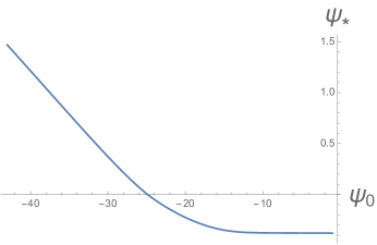
Figure 10: The value of $\psi_{*}$ as a function of $\psi_{0}$.

For $\psi_{0}<-42$, the condition (48) is never satisfied, indicating that the inflaton field overshoots the entire slow-roll region. We note also that there is a critical value of $\psi_{0}$, $\psi_{\rm cr}\simeq-24.8$, above which $\psi_{*}$ is negative and slow-roll starts before the inflaton reaches the inflection point. For later use we also give the slope of the curve in Fig. 10 at $\psi_{0}=\psi_{\rm cr}$:

$$\left.\frac{{\rm d}\psi_{*}}{{\rm d}\psi_{0}}\right|_{\psi_{0}\simeq\psi_{\rm cr}}\simeq-0.06.$$ (49)

5.2 The number of e-folds

The number of e-folds of slow-roll inflation can now be found from

$$N_{e}\approx-\int_{\phi_{*}}^{\phi_{e}}d\phi\frac{U(\phi)}{U^{\prime}(\phi)},$$ (50)

where $\phi_{*}=(2U_{\rm I}/3|{U_{\rm I}^{\prime\prime\prime}}|)\psi_{*}$ is the value of $\phi$ corresponding to $\psi_{*}$. As before, we replace the upper bound of integration by $\infty$ and approximate $U(\phi)$ by $U_{\rm I}$ in the numerator. However, we can no longer neglect the linear term in the potential, since otherwise the integral would diverge at $\phi=0$. Thus we obtain

$$N_{e}\approx-U_{\rm I}\int_{\phi_{*}}^{\infty}\frac{d\phi}{{U_{\rm I}^{\prime}}+\frac{1}{2}{U_{\rm I}}^{\prime\prime\prime}\phi^{2}}=\frac{N_{\rm max}}{2}\left[1-\frac{2}{\pi}\arctan\left(\frac{N_{\rm max}}{3\pi}\psi_{*}\right)\right].$$ (51)

For $\psi_{*}<0$ and $|\psi_{*}|\gg 3\pi/N_{\rm max}$, we can use $\arctan(-x)\approx-\pi/2+x^{-1}$, which gives

$$N_{e}\approx N_{\rm max}-\frac{3}{|\psi_{*}|}.$$ (52)

With $N_{\rm max}\gtrsim 100$, the second term in (52) can be significant only for $|\psi_{*}|\lesssim 0.1$. From the graph in Fig. 10 we see that this is satisfied only in a narrow range $\Delta\psi_{0}\sim 1$ around $\psi_{0}=\psi_{\rm cr}$. We thus conclude that $N_{e}\approx N_{\rm max}$ in most of the range

$$\psi_{\rm cr}<\psi_{0}\lesssim-1.$$ (53)

We shall call it the target range.

Similarly, for positive $\psi_{*}\gg 3\pi/N_{\rm max}$ we find

$$N_{e}\approx\frac{3}{\psi_{*}}.$$ (54)

In order to have $N_{e}\gtrsim 50$, we need $\psi_{*}\lesssim 0.1$, and once again this is satisfied only in a narrow range near $\psi_{\rm cr}$.

We calculated numerically $N_{e}$ as a function of $\psi_{0}$ for several values of $q$. The results are shown in Fig.11. We see that large values of $N_{e}\geq 50$ are reached only for $q\leq 0.03$. For such values of $q$, $N_{e}\approx N_{\rm max}$ in almost the entire target range and $N_{e}$ is negligibly small outside of this range. This is in full agreement with the above analysis.

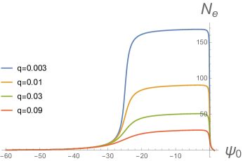
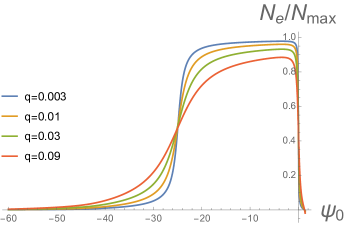
Figure 11: The number of e-folds $N_{e}$ as a function of $\psi_{0}$ for several values of $q$ (left panel) and $N_{e}/N_{\rm max}$ (right panel).

We now comment on the validity of the approximation that we used to neglect the last term in Eq. (42). This term can be significant when $|\psi_{*}|\lesssim\sqrt{q}\approx 10/N_{\rm max}$, which corresponds to a narrow range of $\psi_{0}$ around $\psi_{\rm cr}$. Using Eq. (49) we can estimate this range as

$$\Delta\psi_{0}\sim\left|\frac{d\psi_{*}}{d\psi_{0}}(\psi_{\rm cr})\right|^{-1}\frac{10}{N_{\rm max}}\sim\frac{170}{N_{\rm max}}.$$ (55)

This is precisely the range where $N_{e}$ in Eq. (51) is significantly different from either $N_{\rm max}$ or 0. For $\psi_{0}$ in this range, Eq. (51) for $N_{e}$ may not be very accurate, but we expect that $N_{e}$ interpolates between $N_{\rm max}$ and 0 over this range of $\psi_{0}$, so its qualitative behavior should be well represented by (51).

5.3 Relation to earlier work

The issue of overshooting in slow-roll inflation after tunneling has been discussed earlier by a number of authors Susskind ; Dutta . Freivogel et al Susskind assumed that the exit from tunneling is described by a potential with a linear slope, followed by a flat slow-roll region. Dutta et al Dutta considered power-law exit potentials, $U(\phi)\propto\phi^{n}$ with $n=1,2,3,4$. The main conclusion following from this work is that if $\phi$ starts with some initial value $\phi_{0}$, it overshoots by an amount $\sim\phi_{0}$ into the slow-roll region.

In our context this would imply that tunnelings with initial values $\psi_{0}\lesssim-1$ overshoot most, if not all, of the slow-roll region. We find, however, that there is essentially no overshoot if the bubble nucleates with $\psi_{0}$ in a much wider range, $-25\lesssim\psi_{0}\lesssim 0$. The reason for this discrepancy may be that both Refs. Susskind and Dutta assumed that $U_{\rm I}\ll U(\phi_{0})$. We find that, on the contrary, $U_{\rm I}$ is typically rather close to $U(\phi_{0})$, $U(\phi_{0})-U_{\rm I}\ll U_{\rm I}$.

5.4 Probability of inflation

We can now estimate the probability for a randomly chosen inflection point $\phi_{\rm I}$ in the landscape to be a site of slow-roll inflation. Inflation is possible only if the field tunnels out of the false vacuum to a point within the target range of $\phi_{\rm I}$. The size of the target range is $\Delta\phi_{\rm target}\sim 25\Lambda^{3}$, while the distribution of the nucleation points has the width $\Delta\phi_{0}\sim 0.4\Lambda$. For $\Lambda\ll 0.1$, we have $\Delta\phi_{\rm target}\ll\Delta\phi_{0}$, and the probability for $\phi_{0}$ to be in the target range is

$$P_{\rm target}\sim\frac{\Delta\phi_{\rm target}}{\Delta\phi_{0}}\sim 60\Lambda^{2}\ll 1.$$ (56)

For most of inflection points, the tunneling then occurs outside the target range, so the inflaton overshoots and inflation does not happen. On the other hand, for inflection points where $\phi_{0}$ is in the target range, inflation typically occurs over the entire slow-roll region, so $N_{e}\approx N_{\rm max}$. Since $\phi_{0}$ is uncorrelated with with $N_{\rm max}$ for $N_{\rm max}\gg 1$, we expect that the probability distribution for $N_{e}$ is (almost) the same as that for $N_{\rm max}$. The latter distribution has been calculated in Ref. MVY ,

$$P(N_{\rm max})dN_{\rm max}\approx{2\Lambda^{4}}\frac{dN_{\rm max}}{N_{\rm max}^{3}}.$$ (57)

Using Eqs. (56) and (57), we can now find the probability that a given inflection point supports inflation with $N_{e}>N$ e-folds,

$$P(>N)\sim P_{\rm target}\int_{N}^{\infty}P(N_{\rm max})dN_{\rm max}\sim\frac{60\Lambda^{6}}{N^{2}}.$$ (58)

With $N\gtrsim 100$ and $\Lambda\ll 1$, this probability is rather small. In our view, however, this is not an argument against the random Gaussian landscape model.

Observational predictions of the model are based on landscape realizations with a large number of e-folds, sufficient to solve the flatness problem and to allow for structure formation. All such realizations have $\phi_{0}$ in the target range. Most of them have $N_{e}\approx N_{\rm max}$ and exhibit universal behavior. If the observable scales lie within the slow-roll range, the spectral index $n_{s}$ is related to $N_{\rm max}$ by Eq. (14) and its distribution is given by Eq. (18). The observed value of $n_{s}\approx 0.97$ is in the mid-range of this distribution, as discussed in MVY . Hence a random $1D$ Gaussian landscape is consistent with observations.

5.5 Spatial curvature

Since the interior geometry of the bubble is an open FRW universe, the curvature parameter is nonzero and may have an observable effect Susskind . At the present time this parameter is given by

$$\Omega_{K}\simeq e^{-2N_{e}}\left(\frac{a_{\rm end}H_{\rm end}}{a_{p}H_{p}}\right)^{2},$$ (59)

where the subscripts “end” and “p” represent the values at the end of inflation and at present, respectively. Hereafter, we assume instantaneous reheating and GUT scale inflation to give reference values. Then we have $\ln\Omega_{K}=-2(N_{e}-62)$.

The Planck collaboration puts an upper bound on $\Omega_{K}$ at $\Omega_{K}<10^{-2}$, which requires

$$N_{e}\gtrsim 64.$$ (60)

On the other hand, a detection of spatial curvature is probably possible only if $\Omega_{K}\gtrsim 10^{-4}$, or

$$N_{e}\lesssim 67.$$ (61)

Naively, we could use Eq. (57) to calculate the probability for $N_{e}$ to be within the range defined by these bounds. This would give

$$P(64<N_{e}<67)=\frac{\int_{64}^{67}dN_{e}/N_{e}^{3}}{\int_{64}^{\infty}dN_{e}/N_{e}^{3}}\approx 2.5\%.$$ (62)

We should note, however, that $N_{e}$ is correlated with $N_{\rm max}$, which is in turn related to the spectral index $n_{s}$ by Eq. (14). With the observed value of $n_{s}\approx 0.97$, we should have $N_{\rm max}\approx 120$. Hence, in order to have observable curvature, $N_{e}$ has to be significantly smaller than $N_{max}$. This is possible only if the tunneling point $\psi_{0}$ happens to be very close to the critical value $\psi_{\rm cr}$.

For $\lvert\psi_{*}\rvert\ll 3\pi/N_{\rm max}$, we can approximate Eq. (51) as

$$N_{e}\simeq\frac{N_{\rm max}}{2}\left[1-\frac{2N_{\rm max}}{3\pi^{2}}\psi_{*}\right].$$ (63)

The range of $\psi_{0}$ corresponding to the number of e-folds $N_{e}$ in the range of interest, $\Delta N_{e}\approx 3$, is then given by

$$\Delta\psi_{0}=\frac{d\psi_{0}}{d\psi_{*}}\frac{d\psi_{*}}{dN_{e}}\Delta N_{e},$$ (64)

where the derivatives are evaluated at $\psi_{*}=0$. Using Eqs. (49) and (63) we find $\Delta\psi_{0}\approx 500N_{\rm max}^{-2}$ and

$$P(64<N_{e}<67)\approx\frac{\Delta\psi_{0}}{\psi_{\rm cr}}\approx 1.4\times 10^{-3}\left(\frac{N_{\rm max}}{120}\right)^{-2}.$$ (65)

We thus see that the probability for the curvature to be smaller than the present upper bound but above the future detection limit is rather small.

6 Conclusions

We used numerical simulations to study bubble nucleation by quantum tunneling in random Gaussian potentials. We were particularly interested in slow-roll inflation after the tunneling. For a potential with a correlation length $\Lambda\ll 1$, this typically occurs near a flat inflection point $\phi_{\rm I}$, characterized by $N_{\rm max}\gg 1$. We sampled a large number of randomly generated potentials with flat inflection points and found that a substantial fraction of them (about a half) allow for tunneling from the false vacuum to the neighborhood of $\phi_{\rm I}$. For each tunneling we found the initial value $\phi_{0}$ of the inflaton field in the bubble by solving the Euclidean field equation for the instanton. The resulting distribution is peaked at $\phi_{0}\sim-0.1\Lambda$, where the inflection point is taken to be at $\phi=0$ and the positive direction of $\phi$ is taken to be towards the “true” vacuum. The width of the distribution is $\sim 0.4\Lambda$ and is much larger than the size of the region where slow-roll inflation is possible, $\Delta\phi_{\rm sr}\sim\Lambda^{3}$. This indicates that most of the tunnelings take the field $\phi$ outside of the slow-roll range.

We developed a semi-analytic technique to study the evolution of $\phi$ after tunneling. Our main conclusions can be stated as follows. If the bubble nucleates with $\phi_{0}$ outside the slow-roll range, the field starts rolling fast (after a brief curvature-dominated period) and may overshoot part or all of the slow-roll region, or it may miss this region altogether. We find that if $\phi_{0}$ is in the range

$$\phi_{\rm cr}\lesssim\phi_{0}\lesssim 0,$$ (66)

where $\phi_{\rm cr}\sim-25\Lambda^{3}$, then the field slows down and undergoes a nearly maximal number of inflationary e-folds, $N_{e}\approx N_{\rm max}$. On either side of the range (66), $N_{e}$ drops towards zero within a distance $\Delta\phi_{0}\sim\Lambda^{3}$. The probability distribution for $N_{e}$ has the same power-law form as that for $N_{\rm max}$,

$$P(N_{e})\propto N_{e}^{-3}.$$ (67)

The distribution for the spectral index $n_{s}$ is then given by Eq. (18) and is consistent with the observed value.

We also discussed the prospects for observational detection of nonzero spatial curvature $\Omega_{K}$, which is related to the number of e-folds $N_{e}$. These prospects are not very good, because the observational lower bound on $N_{e}$ is pretty close to the upper bound that would make observational detection possible. Using the distribution (67), we found that the probability for a random observer in the multiverse to detect spatial curvature between these two bounds is $2.5\%$. This estimate changes, however, if we take into account one more data point that is available to us: the measurement of the spectral index of density perturbations: $n_{s}\approx 0.97$. In a small-field Gaussian landscape, $n_{s}$ is rigidly related to $N_{\rm max}$, and the observed value implies $N_{\rm max}\approx 120$. On the other hand, the bound for future detectability requires that $N_{e}\lesssim 67$, which is significantly smaller than $N_{\rm max}$. This situation is possible only if the tunneling point $\phi_{0}$ is very close to $\phi_{\rm cr}$ (within a range $\Delta\phi_{0}\sim\Lambda^{3}$, where $N_{e}$ interpolates between $N_{\rm max}$ and 0). Our estimate for the probability of this to happen is $\sim 10^{-3}$. The bottom line is that the probability of detecting spatial curvature is pretty low if we live in a small-field random Gaussian landscape.

We finally comment on some limitations of our analysis. The distribution for $\phi_{0}$ may have some additional factors, due to the probability measure of the multiverse. These factors may depend on the tunneling transition rates between different vacua and on the correlation between the tunneling action and $\phi_{0}$. This issue is entangled with the measure problem, which at present has no definitive solution and may require some new ideas to be resolved.

Another serious limitation is that we restricted our analysis to a one-dimensional landscape. On the other hand, in multi-dimensional models parts of the landscape where slow-roll inflation is possible may be effectively one-dimensional, with only one of the fields having a nearly flat potential, due to an approximate shift symmetry. In lieu of detailed information about the landscape, it may then be a reasonable approximation to consider such effective $1D$ potentials as samples of a random Gaussian field. We note also that the methods we used here may have a wider applicability. In Ref. MVY we indicated some directions in which these methods can be extended to multi-dimensional landscapes.

7 Acknowledgement

This work is supported by the National Science Foundation under grant 1518742. M.Y. is supported by the JSPS Research Fellowships for Young Scientists.

Appendix A Validity of the interpolation method

In the main part of this paper, we generate the values of potential at equally spaced points $\phi_{i}$ ($i=1,2,3,\dots n$) according to the joint distribution function $P(U_{1},U_{2},\ldots,U_{n})$ obtained from correlation function in Eq. (1). Here we defined $U_{i}=U(\phi_{i})$. We then smoothly interpolate these points to obtain $\tilde{U}(\phi)$. The value of $U(\phi)$ at any point is still a random variable. We can calculate the distribution of $U(\phi)$ with the prior knowledge of $\{U_{1},\ldots,U_{n}\}$. To do so, we again calculate the joint distribution $P(U_{1},U_{2},\ldots,U_{n},U(\phi))$ using the correlation function. We then calculate the conditional distribution of $U(\phi)$ using

$$P(U(\phi)|U_{1},\ldots,U_{n})=\frac{P(U_{1},U_{2},\ldots,U_{n},U(\phi))}{P(U_{1},U_{2},\ldots,U_{n})}.$$ (68)

To do this calculation let us define

$$M_{ij}\equiv\left<U(\phi_{i})U(\phi_{j})\right>~{},$$ (69)

$$M_{0i}=M_{i0}\equiv\left<U(\phi_{i})U(\phi)\right>~{},$$ (70)

$$M_{00}\equiv\left<U(\phi)U(\phi)\right>,$$ (71)

where $i,j=1,2,3,\dots,n$. Equation (68) simplifies to

$$P(U(\phi)|U_{1},\ldots,U_{n})\propto\exp\left[-\frac{1}{2M^{-1}_{00}}\left(U(\phi)+\sum_{j=1}^{n}M^{-1}_{0j}U(\phi_{j})/M^{-1}_{00}\right)\right].$$ (72)

Therefore, the mean value $\left<U(\phi)\right>$ and width $\sigma$ are given by

$$\left<U(\phi)\right>=-\sum_{j=1}^{n}M^{-1}_{0j}U(\phi_{j})/M^{-1}_{00},$$ (73)

$$\sigma=\sqrt{M^{-1}_{00}}.$$ (74)

We plot the interpolating function $\tilde{U}(\phi)$ and $\left<U(\phi)\right>$ and $2\sigma$ region according to Eq. (74) in Fig. 12. The $2\sigma$ region is so narrow that we can not see the difference between the interpolating function and mean value Eq. (73) when the number of points per correlation length is larger than or equal to two. This result justifies the validity of interpolation method. In the main part of this paper, we take the number of points per correlation length as four and set $U(\phi)=\tilde{U}(\phi)$.

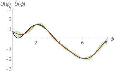
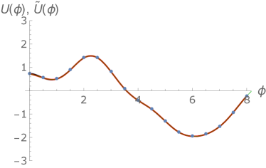
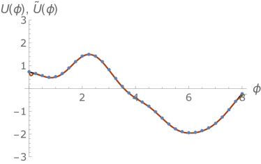
Figure 12: Plots of realizations of potentials and their interpolating functions. The dots represent realizations of potentials and the black lines are the interpolating functions. The number of points per unit correlation length is taken to be $1$ (upper left panel), $2$ (upper right panel), and $4$ (lower panel). The red lines are plotted by Eq. (73) and the green regions are its $2\sigma$ region given by Eq. (74).

Appendix B Cases of multiple instantons

In this section we discuss the non-uniqueness of the instantons of one-dimensional potentials. We need to solve Eq. (19) with the boundary conditions $\phi^{\prime}(0)=0$ and $\lim_{r\rightarrow\infty}\phi(r)=\phi_{\rm fv}$. This is equivalent to the motion of a particle in a one-dimensional upside-down potential, with $r$ playing the role of time. One can tune the value of the field at the center of the instanton $\phi_{0}=\phi(0)$, so that starting from rest it ends up at rest at infinity. Using a simple argument given by Coleman , this is always possible. If $U(\phi_{0})>U_{\rm fv}$ the field can never reach the false vacuum. On the other hand, if $\phi_{0}$ is too close to the true vacuum, it stays there for a while until the effect of the dissipating middle term is negligible. Without this dissipation, it will pass the false vacuum, and hence in some place between these two extreme cases it must land on the false vacuum. This suggests that the closer we start to the true vacuum, the less the dissipation is. However, this is not always the case, as shown in Fig.13.

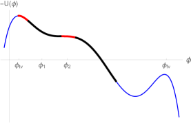
Figure 13: An example of a potential which allows for more than one instanton solution.

Here we show in black the values of $\phi_{0}$ where the field never gets to the false vacuum and use red for points where the field crosses the false vacuum in a finite time. Let’s focus on $\phi_{0}=\phi_{1}$ and $\phi_{0}=\phi_{2}$. The instanton starting at $\phi_{1}$ moves faster than the one starting at $\phi_{2}$ due to the larger gradient at $\phi_{1}$. Hence, it loses more “energy” to the dissipative middle term. The difference between the energy losses can be more than $U(\phi_{1})-U(\phi_{2})$, and hence $\phi_{0}=\phi_{2}$ overshoots while $\phi_{0}=\phi_{1}$ undershoots. At the boundary of red and black regions, there are points that satisfy the boundary conditions. For example in this case there are three such solutions. This shows that new instantons are created in pairs and (except for measure zero set) there is always an odd number of instantons. Let’s mark the instantons from left to right by 1, 2, …. Although we do not have a proof, our numerical solutions for thousands of instantons suggest that the instantons with even numbers have higher actions and are always sub-dominant. We do not know if these instantons have the right number of negative modes and whether they contribute to tunneling at all.

Appendix C Possibility of favorable tunneling to far away minima

In this appendix we present another new and counter-intuitive feature of tunneling in theories with one field. We show that it is possible for a metastable vacuum to decay dominantly to minima which are further away rather than the closer ones. It is not difficult to find cases with two vacua, one on the left and one on the right of a given metastable vacuum, where tunneling to the further away minimum is dominant granted that the barrier separating them is lower. What is non-intuitive is the existence of cases where both minima are on the same side of a false vacuum and the decay to the close minimum is suppressed. One such example is shown in Fig.14.

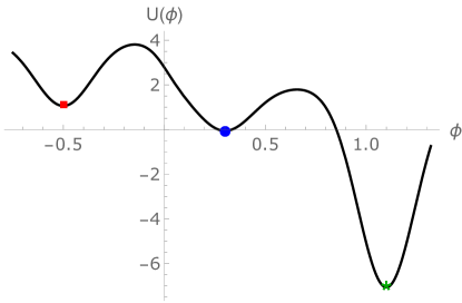
Figure 14: An example of a potential in which decay to the further away minimum is dominant. The metastable vacuum on the left (red square) can decay both to the middle (blue circle) and the right (green star) minimum. The action to the former is around 297 and the latter around 62. Hence, the left vacuum dominantly decays directly to the vacuum on the right.

If there was not a minimum in the middle of the right and left minima, there would always be an instanton that carries the decay to the vacuum on the right. However, if the minimum in the middle (blue circle minimum) is not very deep, it does not effect this instanton much. According to Coleman, there is always an instanton that causes decay to the blue circle minimum. However, this vacuum is nearly degenerate with the one on the left, so we expect it to have a large action and hence to be subdominant.

References

- (1) R. Bousso and J. Polchinski, “Quantization of four form fluxes and dynamical neutralization of the cosmological constant,” JHEP 0006, 006 (2000) [hep-th/0004134].
- (2) L. Susskind, “The Anthropic landscape of string theory,” In *Carr, Bernard (ed.): Universe or multiverse?* 247-266 [hep-th/0302219].
- (3) M. Tegmark, “What does inflation really predict?,” JCAP 0504, 001 (2005) [astro-ph/0410281].
- (4) A. Aazami and R. Easther, “Cosmology from random multifield potentials,” JCAP 0603, 013 (2006) [hep-th/0512050].
- (5) J. Frazer and A. R. Liddle, “Exploring a string-like landscape,” JCAP 1102, 026 (2011) [arXiv:1101.1619 [astro-ph.CO]].
- (6) D. Battefeld, T. Battefeld and S. Schulz, “On the Unlikeliness of Multi-Field Inflation: Bounded Random Potentials and our Vacuum,” JCAP 1206, 034 (2012) [arXiv:1203.3941 [hep-th]].
- (7) L. McAllister, S. Renaux-Petel and G. Xu, “A Statistical Approach to Multifield Inflation: Many-field Perturbations Beyond Slow Roll,” JCAP 1210, 046 (2012) [arXiv:1207.0317 [astro-ph.CO]].
- (8) I. S. Yang, “Probability of Slowroll Inflation in the Multiverse,” Phys. Rev. D 86, 103537 (2012) [arXiv:1208.3821 [hep-th]].
- (9) F. G. Pedro and A. Westphal, “The Scale of Inflation in the Landscape,” Phys. Lett. B 739, 439 (2014) [arXiv:1303.3224 [hep-th]].
- (10) M. C. D. Marsh, L. McAllister, E. Pajer and T. Wrase, “Charting an Inflationary Landscape with Random Matrix Theory,” JCAP 1311, 040 (2013) [arXiv:1307.3559 [hep-th]].
- (11) T. C. Bachlechner, “On Gaussian Random Supergravity,” JHEP 1404, 054 (2014) [arXiv:1401.6187 [hep-th]].
- (12) G. Wang and T. Battefeld, “Vacuum Selection on Axionic Landscapes,” arXiv:1512.04224 [hep-th]..
- (13) A. Masoumi and A. Vilenkin, “Vacuum statistics and stability in axionic landscapes,” JCAP 1603, no. 03, 054 (2016) [arXiv:1601.01662 [gr-qc]].
- (14) B. Freivogel, R. Gobbetti, E. Pajer and I. S. Yang, “Inflation on a Slippery Slope,” arXiv:1608.00041 [hep-th].
- (15) F. G. Pedro and A. Westphal, “Inflation with a graceful exit in a random landscape,” arXiv:1611.07059 [hep-th].
- (16) R. Easther, A. H. Guth and A. Masoumi, “Prevalence of vacua in random Gaussian landscapes”, in preparation.
- (17) A. Masoumi, A. Vilenkin and M. Yamada, “Inflation in random Gaussian landscapes,” arXiv:1612.03960 [hep-th].
- (18) A. D. Linde and A. Westphal, “Accidental Inflation in String Theory,” JCAP 0803, 005 (2008) [arXiv:0712.1610 [hep-th]].
- (19) A. J. Bray and D. S. Dean, “Statistics of critical points of Gaussian fields on large-dimensional spaces,” Phys. Rev. Lett. 98, 150201 (2007).
- (20) T. C. Bachlechner, K. Eckerle, O. Janssen and M. Kleban, “Axions of Evil,” arXiv:1703.00453 [hep-th].
- (21) D. Baumann, A. Dymarsky, I. R. Klebanov and L. McAllister, “Towards an Explicit Model of D-brane Inflation,” JCAP 0801, 024 (2008) [arXiv:0706.0360 [hep-th]].
- (22) S. R. Coleman, “The Fate of the False Vacuum. 1. Semiclassical Theory,” Phys. Rev. D 15, 2929 (1977) Erratum: [Phys. Rev. D 16, 1248 (1977)]. doi:10.1103/PhysRevD.15.2929, 10.1103/PhysRevD.16.1248
- (23) B. Freivogel, “Making predictions in the multiverse,” Class. Quant. Grav. 28, 204007 (2011) doi:10.1088/0264-9381/28/20/204007 [arXiv:1105.0244 [hep-th]].
- (24) A. De Simone, A. H. Guth, M. P. Salem and A. Vilenkin, “Predicting the cosmological constant with the scale-factor cutoff measure,” Phys. Rev. D 78, 063520 (2008) [arXiv:0805.2173 [hep-th]].
- (25) R. Bousso, B. Freivogel and I. S. Yang, “Properties of the scale factor measure,” Phys. Rev. D 79, 063513 (2009) [arXiv:0808.3770 [hep-th]].
- (26) J. Garriga, D. Schwartz-Perlov, A. Vilenkin and S. Winitzki, JCAP 0601, 017 (2006) [hep-th/0509184].
- (27) B. Freivogel, M. Kleban, M. Rodriguez Martinez and L. Susskind, “Observational consequences of a landscape,” JHEP 0603, 039 (2006) [hep-th/0505232].
- (28) K. Dutta, P. M. Vaudrevange and A. Westphal, “The Overshoot Problem in Inflation after Tunneling,” JCAP 1201, 026 (2012) [arXiv:1109.5182 [hep-th]].