Solution properties of a 3D stochastic Euler fluid equation

Abstract.

We prove local well-posedness in regular spaces and a Beale-Kato-Majda blow-up criterion for a recently derived stochastic model of the 3D Euler fluid equation for incompressible flow. This model describes incompressible fluid motions whose Lagrangian particle paths follow a stochastic process with cylindrical noise and also satisfy Newton’s 2nd Law in every Lagrangian domain.

.

1. Introduction

The present paper shows that two important analytical properties of deterministic Euler fluid dynamics in three dimensions possess close counterparts in the stochastic Euler fluid model introduced in [21]. The first of these analytical properties is the local-in-time existence and uniqueness of deterministic Euler fluid flows. The second property is a criterion for blow-up in finite time due to Beale, Kato and Majda [1]. For a historical review of these two fundamental analytical properties for deterministic Euler fluid dynamics, see, e.g., [19]. We believe this fidelity of the stochastic model of [21] investigated here with the analytical properties of the deterministic case bodes well for the potential use of this model in, e.g., uncertainty quantification of either observed, or numerically simulated fluid flows. The need and inspiration for such a model can be illustrated, for example, by examining data from satellite observations collected in the National Oceanic and Atmospheric Administration (NOAA) “Global Drifter Program”, a compilation of which is shown in Figure 1.1.

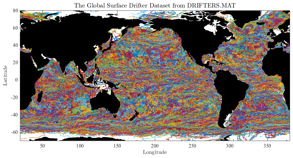
Figure 1.1. This figure shows latitude and longitude of Lagrangian trajectories of drifters on the ocean surface driven by the wind and ocean currents, as compiled from satellite observations by the National Oceanic and Atmospheric Administration Global Drifter Program. Each colour corresponds to a different drifter, see [33]. Upon looking carefully at the individual Lagrangian paths in this figure, one sees that each of them evolves as a mean drift flow, composed with an erratic flow comprising rapid fluctuations around the mean.

Figure 1.1 (courtesy of [33]) displays the global array of surface drifter displacement trajectories from the National Oceanic and Atmospheric Administration’s “Global Drifter Program” (www.aoml.noaa.gov/phod/dac). In total, more than 10,000 drifters have been deployed since 1979, representing nearly 30 million data points of positions along the Lagrangian paths of the drifters at six-hour intervals. This large spatiotemporal data set is a major source of information regarding ocean circulation, which in turn is an important component of the global climate system. For a recent discussion, see for example [49]. This data set of spatiotemporal observations from satellites of the spatial paths of objects drifting near the surface of the ocean provides inspiration for further development of data-driven stochastic models of fluid dynamics of the type discussed in the present paper.

Inspired by this drifter data, the present paper investigates the existence, uniqueness and singularity properties of a recently derived stochastic model of the Euler fluid equations for incompressible flow [21] that is consistent with this data. For this purpose, we combine methods from geometric mechanics, functional analysis and stochastic analysis. In the model under investigation, one assumes that the Lagrangian particle paths in the fluid motion $x_{t}=\eta_{t}(X)$ with initial position $X\in\mathbb{R}^{3}$ each follow a Stratonovich stochastic process given by

$$\mathsf{d}\eta_{t}(X)=u(\eta_{t}(X),t)dt+\sum_{i}\xi_{i}(\eta_{t}(X))\circ dB^{i}_{t}\,.$$ (1.1)

This approach immediately introduces the issue of spatial correlations.

In particular, an important feature of the data in Figure 1.1 is that the ocean currents show up as persistent spatial correlations, easily recognised visually as spatial regions in which the colours representing individual paths tend to concentrate. To capture this feature, we transform the Lagrangian trajectory description (1.1) into the spatial representation of the Eulerian transport velocity given by the Stratonovich stochastic vector field,

$$\mathsf{dy}_{t}(x)=u(x,t)dt+\sum_{i}\xi_{i}(x)\circ dB^{i}_{t}=\mathsf{d}\eta_{t}\,\eta_{t}^{-1}(x)\,.$$ (1.2)

In equations (1.1) and (1.2), the $B_{t}^{i}$ with $i\in\mathbb{N}$ are scalar independent Brownian motions, and the $\xi_{i}(x)$ represent the spatial correlations which may be obtained as eigenvectors of the two-point velocity-velocity correlation matrix $C_{ij}(x,y)$, $i,j=1,2,\dots,N$, as an integral operator. Namely,

$$\sum_{j}\int C_{ij}(x,y)\xi_{j}(y)dy=\lambda\xi_{i}(x)\,.$$ (1.3)

These correlation eigenvectors exhibit a spectrum of spatial scales for the trajectories of the drifters, indicating the variety of spatiotemporal scales in the evolution of the ocean currents which transport the drifters. This feature of the data is worthy of further study. In what follows, we will assume that the velocity correlation eigenvectors $\xi_{i}(x)$ with $i=1,\dots,N$ have been determined by reliable data assimilation procedures, so we may take them to be prescribed, divergence-free, three-dimensional vector functions. For explicit examples of the process of determining the $\xi_{i}(x)$ eigenvectors at coarse resolution from finely resolved numerical simulations, see [5, 6]. For an extension of this method to include non-stationary correlation statistics, see [18].

A rigorous analysis of the stochastic process $\eta_{t}$ in (1.1) is under way by the authors. Following from classical results (e.g., [29, 30]), we show in a forthcoming paper that $\eta_{t}$ is a temporally stochastic curve on the manifold of smooth invertible maps with smooth inverses (i.e., diffeomorphisms). Thus, although the time dependence of $\eta_{t}$ in (1.1) is not differentiable, its spatial dependence is smooth. The stochastic process $\mathsf{d}\eta_{t}(X)$ in (1.1) is also the pullback by the diffeomorphism $\eta_{t}$ of the stochastic vector field $\mathsf{dy}_{t}(x)$ in (1.2). That is, $\eta^{*}_{t}\mathsf{dy}_{t}(x)=\mathsf{d}\eta_{t}(X)$, see e.g. [21] for details. Conversely, the stochastic vector field in (1.2) is the Eulerian representation in fixed spatial coordinates $x$ of the stochastic process in (1.1) for the Lagrangian fluid parcel paths, labelled by their Lagrangian coordinates $X$.

The expression for the Lagrangian trajectories in equation (1.1) is clearly in accord with the observed behaviour of the Lagrangian trajectories displayed in Figure 1.1. Moreover, the expression (1.2) for the corresponding Eulerian transport velocity has been derived recently in [7] by using multi-time homogenisation methods for Lagrangian trajectories corresponding to solutions of the deterministic Euler equations, in the asymptotic limit of time-scale separation between the mean and fluctuating flow. In particular, the fluctuating dynamics in the second term in (1.2) has been shown in [7] to affect the mean flow. Thus, beyond being potentially useful as a means of uncertainty quantification, the decomposition in (1.2) represents a bona fide decomposition of the Eulerian fluid velocity into mean plus fluctuating components.

The approach of incorporating uncertainties in incompressible fluid motion via stochastic Lagrangian fluid trajectories as in equation (1.1) has several precedents, including for example, [2, 39, 38]. However, the Eulerian fluid representation in (1.2) will lead us next to a stochastic partial differential equation (SPDE) for the Eulerian drift velocity $u$ driven by cylindrical noise represented by the Stratonovich term in (1.2) which differs from the Eulerian equations treated in these precedents. For detailed discussions of SPDE with cylindrical noise, see [8, 42, 44, 48].

Stochastic Euler fluid equations.

As shown in [21] via Hamilton’s principle and rederived via Newton’s Law in Appendix A of the present paper, the stochastic Euler fluid equations we shall study in this paper may be represented in Kelvin circulation theorem form, as

$$\mathsf{d}\oint_{c(t)}{v_{j}}(x,t)\,dx^{j}=\oint_{c(t)}\rho^{-1}F_{j}\,dx^{j}\,,$$ (1.4)

in which the closed loop $c(t)$ follows the Lagrangian stochastic process in (1.1), which means it moves with stochastic Eulerian fluid velocity $\mathsf{dy}_{t}$ in (1.2). In Kelvin’s circulation theorem (1.4), the mass density is denoted as $\rho$, and $F_{j}$ denotes the $j$-th component of the force exerted on the flow. In the present work, the mass density $\rho$ will be assumed to be constant. Notice that the covariant vector with components $v_{j}(x,t)$ in the integrand of (1.4) is not the transport velocity in (1.2). Instead, $v_{j}(x,t)$ is the $j$-th component of the momentum per unit mass. In what follows, the force per unit mass $\rho^{-1}F_{j}=-\rho^{-1}\partial_{j}p$ will be taken to be proportional to the pressure gradient. For this force, the Kelvin loop integral in (1.4) for the stochastic Euler fluid case will be preserved in time for any material loop whose motion is governed by the Stratonovich stochastic process (1.1). That is, equation (1.4) implies, for every rectifiable loop $c\subset\mathbb{R}^{3}$, the momentum per unit mass $v_{t}$ has the property that for all $t\in[0,T]$,

$$\oint_{\eta_{t}(c)}v_{t}\cdot dx=\oint_{c}v_{0}\cdot dx,\quad\ a.s.$$ (1.5)

pathwise Kelvin theorem (1.5) is reminiscent of the Constantin-Iyer Kelvin theorem in [4] which has the beautifully simple implication that smooth Navier-Stokes solutions $u_{t}$ are characterized by the following statistical Kelvin theorem which holds for all loops $\Gamma\subset\mathbb{R}^{3}$,

$$\int_{\Gamma}u_{t}\cdot dx=\mathbb{E}\left[\int_{A_{t}(\Gamma)}u_{0}\cdot dx\right],$$ (1.6)

where $A_{t}$ is the back-to-labels map for a stochastic flow of a certain forward Itô equation and $\mathbb{E}$ denotes expectation for that flow. Unlike the pathwise Kelvin theorem (1.5) which holds for solutions of the stochastic Euler fluid equations, the Constantin-Iyer Kelvin theorem in (1.6) is completely deterministic; since, the fluid velocity $u_{t}$ is a solution of the Navier-Stokes equations. For more discussion of Kelvin circulation theorems for stochastic Euler fluid equations see [10].

In the case of the stochastic Euler fluid treated here in Euclidean coordinates, applying the Stokes theorem to the Kelvin loop integral in (1.4) yields the equation for $\omega=\mathrm{curl}\,{v}$ proposed in [21], as

$$\mathsf{d}\omega+(\mathsf{dy}_{t}\cdot\nabla)\omega-(\omega\cdot\nabla)\mathsf{dy}_{t}=0\,,\qquad\omega|_{t=0}=\omega_{0}\,,$$ (1.7)

where the loop integral on the right hand side of (1.4) vanishes for pressure forces with constant mass density.

Main results.

This paper shows that two well-known analytical properties of the deterministic 3D Euler fluid equations are preserved under the stochastic modification in (1.7) we study here. First, the 3D stochastic Euler fluid vorticity equation (1.7) is locally well-posed in the sense that it possesses local in time existence and uniqueness of solutions, for initial vorticity in the space $W^{2,2}(\mathbb{R}^{3})$ [11]. See Lichtenstein [32] as mentioned in [17] for a historical precedent for local existence and uniqueness for the Euler fluid equations. Second, the vorticity equations (1.7) also possess a Beale-Kato-Majda (BKM) criterion for blow up which is identical to the one proved for the deterministic Euler fluid equations in [1].

Theorem 1 (Existence and uniqueness).

Given initial vorticity $\omega_{0}\in W^{2,2}\left(\mathbb{T}^{3},\mathbb{R}^{3}\right)$, there exists a local solution in $W^{2,2}$ of the stochastic 3D Euler equations (1.7). Namely, if $\omega^{\left(1\right)},\omega^{\left(2\right)}:\Xi\times\left[0,\tau\right]\times\mathbb{T}^{3}\rightarrow\mathbb{R}^{3}$ are two solutions defined up to the same stopping time $\tau>0$, then $\omega^{\left(1\right)}=\omega^{\left(2\right)}$.

Our result corresponding to the celebrated Beale-Kato-Majda characterization of blow-up [1] is stated in the following.

Theorem 2 (Beale-Kato-Majda criterion for blow up).

Given initial $\omega_{0}\in W^{2,2}\left(\mathbb{T}^{3},\mathbb{R}^{3}\right)$, there exists a stopping time $\tau_{\max}:\Xi\rightarrow\left[0,\infty\right]$ and a process $\omega:\Xi\times[0,\tau_{\max})\times\mathbb{T}^{3}\rightarrow\mathbb{R}^{3}$ with the following properties:

i) ($\omega$ is a solution) The process $t\mapsto\omega\left(t\wedge\tau_{\max},\cdot\right)$ has trajectories that are almost surely in the class $C\left([0,\tau_{\max});W^{2,2}\left(\mathbb{T}^{3};\mathbb{R}^{3}\right)\right)$ and equation (1.7) holds as an identity in $L^{2}\left(\mathbb{T}^{3};\mathbb{R}^{3}\right)$. In addition, $\tau_{\max}$ is the largest stopping time with this property; and

ii) (Beale-Kato-Majda criterion [1]) If $\tau_{\max}<\infty$, then

$$\int_{0}^{\tau_{\max}}\left\|\omega\left(t\right)\right\|_{\infty}dt=+\infty$$

and, in particular, $\lim\sup_{t\uparrow\tau_{\max}}\left\|\omega\left(t\right)\right\|_{\infty}=+\infty$.

Plan of the paper

 

• Section 2 discusses our assumptions and summarizes the main results of the paper.

  • Subsection 2.1 formulates our objectives and sets the notation.

  • Subsection 2.2 discusses the cylindrical noise properties of (1.1) and provides basic bounds on the Lie derivatives needed in proving the main analytical results.

  • Subsection 2.3 provides additional definitions needed in the context of explaining the main results of the paper.

• Section 3 provides proofs of the main results

  • Subsections 3.1 and 3.3 prove the uniqueness properties needed for establishing Theorem 1.

  • Subsection 3.5 introduces a cut-off function which is instrumental in the proof of the BKM theorem for the stochastic Euler equations given in Subsection 3.4.

• Section 4 summarizes the proofs of several key technical results which are summoned in establishing Theorem 1 and Theorem 2.

  • Subsection 4.1 discusses fractional Sobolev regularity in time.

  • Subsection 4.2 provides the a priori bounds needed to prove estimate (3.19).

  • Subsection 4.3 proves the bounds needed to complete the proof that the estimate (3.19) is uniform in time.

  • Subsection 4.4 establishes the key estimates for the bounds involving Lie derivatives that are needed in the proofs.

• Appendix A provides a new derivation of the stochastic Euler equations introduced in [21] from the viewpoint of Newton’s 2nd Law and derives the corresponding Kelvin circulation theorem. The deterministic (resp. stochastic) equations of motion are derived using the pullback of Newton’s 2nd Law by the deterministic (resp. stochastic) diffeomorphism describing the Lagrange-to-Euler map. The Kelvin circulation theorems for both cases are then derived from their corresponding Newtonian 2nd Laws. The importance of the distinction between transport velocity and transported momentum is emphasized in Appendix A for both the deterministic and stochastic Newton’s Laws and Kelvin’s circulation theorems.

2. Assumptions and main results

2.1. Formulating objectives and setting notation

Our aim from now on will be to prove local-in-time existence and uniqueness of regular solutions of the stochastic Euler vorticity equation

$$d\omega+\mathcal{L}_{v}\omega dt+\sum_{k=1}^{\infty}\mathcal{L}_{\xi_{k}}\omega\circ dB_{t}^{k}=0,\qquad\omega|_{t=0}=\omega_{0},$$ (2.1)

which was proposed in [21]. Here, $\mathcal{L}_{v}\omega$ (resp. $\mathcal{L}_{\xi_{k}}\omega$) denotes the Lie derivative with respect to the vector fields $v$ (resp. $\xi_{k}$) as in (A.27) applied to the vorticity vector field. In particular,

$$\mathcal{L}_{\xi_{k}}\omega=(\xi_{k}\cdot\nabla)\omega-(\omega\cdot\nabla)\xi_{k}=\left[\,\xi_{k}\,,\,\omega\,\right].$$ (2.2)

A natural question is whether we should sum only over a finite number of terms or, on the contrary, it is important to have an infinite sum, and not only for generality. An important remark is that a finite number of eigenvectors arises in the relevant case associated to a “data driven” model based on what is resolvable in either numerics of observations; and it would simplify some technical issues (we do not have to assume (2.11) below). However, an infinite sum could be of interest in regularization-by-noise investigations: see an example in [9] (easier than 3D Euler equations) where a singularity is prevented by an infinite dimensional noise. However, it is also true that in some cases a finite dimensional noise is sufficient also for regularization by noise, see examples in [14], [15], [16].

As mentioned in Remark 32, for the case of the Euler fluid equations treated here in Cartesian $\mathbb{R}^{3}$ coordinates, the two velocities denoted $u$ and $v$ in the previous section may be taken to be identical vectors for the case at hand in $\mathbb{R}^{3}$. Consequently, for the remainder of the present work, in a slight abuse of notation, we simply let $v$ denote the both fluid velocity and the momentum per unit mass. Then $\omega=\operatorname{curl}v$ is the vorticity, and $\xi_{k}$ comprise $N$ divergence-free prescribed vector fields, subject to the assumptions stated below. The processes $B^{k}$ with $k\in\mathbb{N}$ are scalar independent Brownian motions. The result we present next will extend the known analogous result for deterministic Euler equations to the stochastic case.

To simplify some of the arguments, we will work on a torus $\mathbb{T}^{3}=\mathbb{R}^{3}/\mathbb{Z}^{3}$. However, the results should also hold in the should also hold in the full space, $\mathbb{R}^{3}$.

The stochastic Euler vorticity equation (2.1) above is stated in Stratonovich form. The corresponding Itô form is

$$d\omega+\mathcal{L}_{v}\omega dt+\sum_{k=1}^{\infty}\mathcal{L}_{\xi_{k}}\,\omega dB_{t}^{k}=\frac{1}{2}\sum_{k=1}^{\infty}\mathcal{L}_{\xi_{k}}^{2}\omega\ dt\,,\qquad\omega|_{t=0}=\omega_{0}\,,$$ (2.3)

where we write

$$\mathcal{L}_{\xi_{k}}^{2}\omega=\mathcal{L}_{\xi_{k}}(\mathcal{L}_{\xi_{k}}\omega)=\left[\xi_{k}\,,[\xi_{k}\,,\,\omega]\right]\,,$$

for the double Lie bracket of the divergence-free vector field $\xi_{k}$ with the vorticity vector field $\omega$. Indeed, let us recall that Stratonovich integral is equal to Itô integral plus one-half of the corresponding cross-variation process:

$$\int_{0}^{t}\mathcal{L}_{\xi_{k}}\omega_{s}\circ dB_{s}^{k}=\int_{0}^{t}\mathcal{L}_{\xi_{k}}\omega_{s}dB_{s}^{k}+\frac{1}{2}\left[\mathcal{L}_{\xi_{k}}\omega,B^{k}\right]_{t}.$$

By the linearity and the space-independence of $B^{k}$, $\left[\mathcal{L}_{\xi_{k}}\omega,B^{k}\right]_{t}=\mathcal{L}_{\xi_{k}}\left[\omega,B^{k}\right]_{t}$. As $\omega_{t}$ has the form $d\omega_{t}=a_{t}dt+\sum_{h}b_{t}^{h}\circ dB_{t}^{h}$, where $B^{h}$ are independent, the cross-variation process $\left[\omega,B^{k}\right]_{t}$ is given by

$$\left[\omega,B^{k}\right]_{t}=\int_{0}^{t}b_{s}^{k}ds.$$

In our case $b_{s}^{k}=-\mathcal{L}_{\xi_{k}}\omega_{s}$, hence

$$\left[\omega,B^{k}\right]_{t}=-\int_{0}^{t}\mathcal{L}_{\xi_{k}}\omega_{s}ds.$$

Finally

$$\mathcal{L}_{\xi_{k}}\left[\omega,B^{k}\right]_{t}=-\int_{0}^{t}\mathcal{L}_{\xi_{k}}^{2}\omega_{s}ds$$

and therefore, in differential form,

$$\mathcal{L}_{\xi_{k}}\omega_{t}\circ dB_{t}^{k}=\mathcal{L}_{\xi_{k}}\omega_{t}\,dB_{t}^{k}-\frac{1}{2}\mathcal{L}_{\xi_{k}}^{2}\omega_{t}dt.$$

Among different possible strategies to study equation (2.3), some of them based on stochastic flows, we present here the extension to the stochastic case of a classical PDE proof, see for instance [26], [35], [36].

The proof is based on a priori estimates in high order Sobolev spaces. The deterministic classical result proves well-posedness in the space $\omega\left(t\right)\in W^{3/2+\epsilon,2}\left(\mathbb{T}^{3};\mathbb{R}^{3}\right)$, for some $\epsilon>0$, when $\omega_{0}$ belongs to the same space. Here we simplify (due to a number of new very non-trivial facts outlined below in section 4.2) and work in the space $\omega\left(t\right)\in W^{2,2}\left(\mathbb{T}^{3};\mathbb{R}^{3}\right)$. Consequently, we may consider $\Delta\omega\left(t\right)$ (to avoid fractional derivatives) and investigate existence and uniqueness in the class of regularity $\Delta\omega\left(t\right)\in L^{2}\left(\mathbb{T}^{3};\mathbb{R}^{3}\right)$.

If $f,g\in L^{2}\left(\mathbb{T}^{3};\mathbb{R}^{3}\right)$, we write $\left\langle f,g\right\rangle=\int_{\mathbb{T}^{3}}f\left(x\right)\cdot g\left(x\right)dx$. We consider the basis of $L^{2}\left(\mathbb{T}^{3};\mathbb{C}\right)$ of functions $\left\{e^{2\pi i\xi\cdot x};\xi\in\mathbb{Z}^{3}\right\}$ and, for every $f\in L^{2}\left(\mathbb{T}^{3};\mathbb{C}\right)$, we introduce the Fourier coefficients $\widehat{f}\left(\xi\right)=\int_{\mathbb{T}^{3}}e^{-2\pi i\xi\cdot x}f\left(x\right)dx$, $\xi\in\mathbb{Z}^{3}$; Parseval identity states that $\int_{\mathbb{T}^{3}}\left|f\left(x\right)\right|^{2}dx=\sum_{\xi\in\mathbb{Z}^{3}}\left|\widehat{f}\left(\xi\right)\right|^{2}$. If $v\in L^{2}\left(\mathbb{T}^{3};\mathbb{R}^{3}\right)$ is a vector field with components $v_{i}$, $i=1,2,3$, we write $\widehat{v}\left(\xi\right)=\int_{\mathbb{T}^{3}}e^{2\pi i\xi\cdot x}v\left(x\right)dx$ and we may easily check using the components that have $\int_{\mathbb{T}^{3}}\left|v\left(x\right)\right|^{2}dx=\sum_{\xi\in\mathbb{Z}^{3}}\left|\widehat{v}\left(\xi\right)\right|^{2}$. Since functions which are partial derivatives of other functions, on the torus, must have zero average, we shall always restrict ourselves to functions $f\in L^{2}\left(\mathbb{T}^{3};\mathbb{C}\right)$ such that $\int_{\mathbb{T}^{3}}f\left(x\right)dx=0$. In this case $\widehat{f}\left(0\right)=0$ and the term with $\xi=0$ does not appear in the sums above.

We introduce, for every $s\geq 0$, the fractional Sobolev space $W^{s,2}\left(\mathbb{T}^{3};\mathbb{C}\right)$ of all $f\in L^{2}\left(\mathbb{T}^{3};\mathbb{C}\right)$ such that

$$\left\|f\right\|_{W^{s,2}}^{2}:=\sum_{\xi\in\mathbb{Z}^{3}\backslash\left\{0\right\}}\left|\xi\right|^{2s}\left|\widehat{f}\left(\xi\right)\right|^{2}<\infty.$$

As stated above, we are assuming zero average functions, hence we have excluded $\xi=0$. We denote by $W_{\sigma}^{s,2}\left(\mathbb{T}^{3},\mathbb{R}^{3}\right)$ the space of all zero mean divergence free (divergence in the sense of distribution) vector fields $v\in L^{2}\left(\mathbb{T}^{3};\mathbb{R}^{3}\right)$ such that all components $v_{i}$, $i=1,2,3$, belong to $W^{s,2}\left(\mathbb{T}^{3};\mathbb{C}\right)$. For a vector field $v\in W_{\sigma}^{s,2}\left(\mathbb{T}^{3},\mathbb{R}^{3}\right)$ the norm $\left\|v\right\|_{W^{s,2}}$ is defined by the identity $\left\|v\right\|_{W_{\sigma}^{s,2}}^{2}=\sum_{i=1}^{3}\left\|v_{i}\right\|_{W^{s,2}}^{2}$, where $\left\|v_{i}\right\|_{W^{s,2}}^{2}$ is defined above. We thus have again $\left\|v\right\|_{W_{\sigma}^{s,2}}^{2}:=\sum_{\xi\in\mathbb{Z}^{3}\backslash\left\{0\right\}}\left|\xi\right|^{2s}\left|\widehat{v}\left(\xi\right)\right|^{2}$. For $f\in W^{s,2}\left(\mathbb{T}^{3};\mathbb{C}\right)$, we denote by $\left(-\Delta\right)^{s/2}f$ the function of $L^{2}\left(\mathbb{T}^{3};\mathbb{C}\right)$ with Fourier coefficients $\left|\xi\right|^{s}\widehat{f}\left(\xi\right)$. Similarly, we write $-\Delta^{-1}f$  for the function having Fourier coefficients $\left|\xi\right|^{-2}\widehat{f}\left(\xi\right)$. We use the same notations for vector fields, meaning that the operations are made componentwise.

The Biot-Savart operator is the reconstruction of a zero mean divergence free vector field $u$ from a divergence free vector field $\omega$ such that $\operatorname{curl}u=\omega$. On the torus it is given by $u=-\operatorname{curl}\Delta^{-1}\omega$. In Fourier components, it is given by $\widehat{u}\left(\xi\right)=\left|\xi\right|^{-2}\xi\times\widehat{\omega}\left(\xi\right)$. We have the following well-known result: for all $s\geq 0$

$$\left\|u\right\|_{W_{\sigma}^{s+1,2}}\leq\left\|\omega\right\|_{W_{\sigma}^{s,2}}.$$ (2.4)

Indeed, using the definition given above of $\left\|u\right\|_{W_{\sigma}^{s+1,2}}^{2}$, the formula which relates $\widehat{u}\left(\xi\right)$ to $\widehat{\omega}\left(\xi\right)$ and the rule $\left|a\times b\right|\leq\left|a\right|\left|b\right|$, we get

$$\left\|u\right\|_{W_{\sigma}^{s+1,2}}^{2}=\sum_{\xi\in\mathbb{Z}^{3}\backslash\left\{0\right\}}\left|\xi\right|^{2s+2}\left|\widehat{u}\left(\xi\right)\right|^{2}=\sum_{\xi\in\mathbb{Z}^{3}\backslash\left\{0\right\}}\left|\xi\right|^{2s+2}\left|\xi\right|^{-4}\left|\xi\times\widehat{\omega}\left(\xi\right)\right|^{2}\leq\sum_{\xi\in\mathbb{Z}^{3}\backslash\left\{0\right\}}\left|\xi\right|^{2s+2}\left|\xi\right|^{-2}\left|\widehat{\omega}\left(\xi\right)\right|^{2}$$

and the latter is precisely equal to $\left\|\omega\right\|_{W_{\sigma}^{s,2}}$, by the definition above.

We shall denote the dual operator of the Lie derivative $\mathcal{L}_{\alpha}$ of a vector field as $\mathcal{L}_{\alpha}^{\ast}$, defined by the identity

$$\left\langle\mathcal{L}_{\alpha}^{\ast}\beta,\gamma\right\rangle=\left\langle\beta,\mathcal{L}_{\alpha}\gamma\right\rangle,$$

for all smooth vector fields $\alpha,\beta,\gamma$. When $\operatorname{div}\alpha=0$ the dual Lie operator is given in vector components by

$$\left(\mathcal{L}_{\alpha}^{\ast}\gamma\right)_{i}:=-\sum_{j}\left(\alpha^{j}\partial_{j}\gamma_{i}+\gamma_{j}\partial_{i}\alpha^{j}\right)\,.$$ (2.5)

2.2. Assumptions on $\left\{\xi_{k}\right\}$ and basic bounds on Lie derivatives

We assume that the vector fields $\xi_{k}:\mathbb{T}^{3}\rightarrow\mathbb{R}^{3}$ are of class $C^{4}$ and satisfy

$$\left\|\sum_{k=1}^{\infty}\mathcal{L}_{\xi_{k}}^{2}f\right\|_{L^{2}}^{2}\leq C\left\|f\right\|_{W^{2,2}}^{2}$$ (2.6)

$$\sum_{k=1}^{\infty}\left\langle\mathcal{L}_{\xi_{k}}f,\mathcal{L}_{\xi_{k}}f\right\rangle\leq C\left\|f\right\|_{W^{2,2}}^{2}$$ (2.7)

for all $f\in W^{2,2}\left(\mathbb{T}^{3};\mathbb{R}^{3}\right)$ and

$$\sum_{k=1}^{\infty}\left\|\xi_{k}\right\|_{W^{3,2}}^{2}<\infty.$$ (2.8)

These properties will be used below, both to give a meaning to the stochastic terms in the equation and to prove certain bounds. In addition, a recurrent energy-type scheme in our proofs requires comparisons of quadratic variations and Stratonovich corrections. Making these comparisons leads to sums of the form $\left\langle\mathcal{L}_{\xi_{k}}^{2}f,f\right\rangle+\left\langle\mathcal{L}_{\xi_{k}}f,\mathcal{L}_{\xi_{k}}f\right\rangle$. In dealing with them, we have observed the validity of two striking bounds, which a priori may look surprising. They are:

$$\left\langle\mathcal{L}_{\xi_{k}}^{2}f,f\right\rangle+\left\langle\mathcal{L}_{\xi_{k}}f,\mathcal{L}_{\xi_{k}}f\right\rangle\leq C_{k}^{\left(0\right)}\left\|f\right\|_{L^{2}}^{2}$$ (2.9)

$$\left\langle\Delta\mathcal{L}_{\xi_{k}}^{2}f,\Delta f\right\rangle+\left\langle\Delta\mathcal{L}_{\xi_{k}}f,\Delta\mathcal{L}_{\xi_{k}}f\right\rangle\leq C_{k}^{\left(2\right)}\left\|f\right\|_{W^{2,2}}^{2},$$ (2.10)

for suitable constants $C_{k}^{\left(0\right)},C_{k}^{\left(2\right)}$. For these estimates to hold, the regularity of $f$ must be, respectively, $W^{2,2}\left(\mathbb{T}^{3};\mathbb{R}^{3}\right)$ and $W^{4,2}\left(\mathbb{T}^{3};\mathbb{R}^{3}\right)$. The proofs of estimates (2.9) and (2.10) are given in Section 4.4 below.

Concerning inequality (2.9), it is clear that the second order terms in $\left\langle\mathcal{L}_{\xi_{k}}^{2}f,f\right\rangle$ and $\left\langle\mathcal{L}_{\xi_{k}}f,\mathcal{L}_{\xi_{k}}f\right\rangle$ will cancel. However, the cancellations among the first order terms are not so obvious. Remarkably, though, these terms do cancel each other, so that only the zero-order terms remain. Similar remarks apply to the other inequality.

In addition, we must assume

$$\sum_{k=1}^{\infty}C_{k}^{\left(0\right)}<\infty,\qquad\sum_{k=1}^{\infty}C_{k}^{\left(2\right)}<\infty.$$ (2.11)

Because the constants $C_{k}^{\left(i\right)}$ are rather complicated, we will not write them explicitly here. In the relevant case of a finite number of $\xi_{k}$’s, there is obviously no need of this assumption. In the case of infinitely many terms, see a sufficient condition in Remark 28 of Section 4.4.

2.3. Statement of the main results

Let $\left\{B^{k}\right\}_{k\in\mathbb{N}}$ be a sequence of independent Brownian motions on a filtered probability space $\left(\Xi,\mathcal{F},\mathcal{F}_{t},P\right)$. We do not use the most common notation $\Omega$ for the probability space, since $\omega$ is the traditional notation for the vorticity. Thus the elementary events will be denoted by $\theta\in\Xi$. Let $\left\{\xi_{k}\right\}_{k\in\mathbb{N}}$ be a sequence of vector fields, satisfying the assumptions of section 2.2. Consider equations (2.3) on $[0,\infty)$.

Definition 3 (Local solution).

A local solution in $W_{\sigma}^{2,2}$ of the stochastic 3D Euler equations (2.3) is given by a pair $\left(\tau,\omega\right)$ consisting of a stopping time $\tau:\Xi\rightarrow[0,\infty)$ and a process $\omega:\Xi\times\left[0,\tau\right]\times\mathbb{T}^{3}\rightarrow\mathbb{R}^{3}$ such that a.e. the trajectory is of class $C\left(\left[0,\tau\right];W_{\sigma}^{2,2}\left(\mathbb{T}^{3};\mathbb{R}^{3}\right)\right)$, $\omega\left(t\wedge\tau,\cdot\right)$, is adapted to $\left(\mathcal{F}_{t}\right)$, and equation (2.3) holds in the usual integral sense; More precisely, for any bounded stopping time $\bar{\tau}\leq\tau$

$$\omega_{\bar{\tau}}-\omega_{0}+\int_{0}^{\bar{\tau}}\mathcal{L}_{v}\omega dt+\sum_{k=1}^{\infty}\int_{0}^{\bar{\tau}}\mathcal{L}_{\xi_{k}}\omega dB_{t}^{k}=\frac{1}{2}\sum_{k=1}^{\infty}\int_{0}^{\bar{\tau}}\mathcal{L}_{\xi_{k}}^{2}\omega\ dt\,$$ (2.12)

holds as an identity in $L^{2}\left(\mathbb{T}^{3};\mathbb{R}^{3}\right)$.

Definition 4 (Maximal solution).

A maximal solution of (2.3) is given by a stopping time $\tau_{\max}:\Xi\rightarrow\left[0,\infty\right]$ and a process $\omega:\Xi\times[0,\tau_{\max})\times\mathbb{T}^{3}\rightarrow\mathbb{R}^{3}$ such that: i) $P\left(\tau_{\max}>0\right)=1$, $\tau_{\max}=\lim_{n\rightarrow\infty}\tau_{n}$ where $\tau_{n}$ is an increasing sequence of stopping times, and ii) $\left(\tau_{n},\omega\right)$ is a local solution for every $n\in\mathbb{N}$; In addition, $\tau_{\max}$ is the largest stopping time with properties i) and ii). In other words, if $(\tau^{\prime},\omega^{\prime})$ is another pair that satisfies i) and ii) and $\omega^{\prime}=\omega$ on $[0,\tau^{\prime}\wedge\tau_{\max}),$ then, $\tau^{\prime}\leq\tau_{\max}$ $P$-almost surely.

Remark 5.

Due to assumptions (2.6) and (2.7) and the regularity of $\omega$, the two terms related to the noise in equation (2.3) are well defined, as elements of $L^{2}\left(\mathbb{T}^{3};\mathbb{R}^{3}\right)$.

Remark 6.

Recall that, for every $\alpha\geq 0$, $\omega\left(t\right)\in W^{\alpha,2}\left(\mathbb{T}^{3};\mathbb{R}^{3}\right)$ implies $v\left(t\right)\in W^{\alpha+1,2}\left(\mathbb{T}^{3};\mathbb{R}^{3}\right)$. Hence solutions in $W^{2,2}$ have paths such that $v\in C\left(\left[0,\tau\right];W^{3,2}\left(\mathbb{T}^{3};\mathbb{R}^{3}\right)\right)$. Moreover, recall that $W^{\alpha,2}\left(\mathbb{T}^{3};\mathbb{R}^{3}\right)\subset C\left(\mathbb{T}^{3};\mathbb{R}^{3}\right)$ for $\alpha>3/2$. Therefore $\omega\cdot\nabla v\in C\left(\left[0,\tau\right]\times\mathbb{T}^{3};\mathbb{R}^{3}\right)$ and $v\cdot\nabla\omega$ is at least in $C\left(\left[0,\tau\right];W^{1,2}\left(\mathbb{T}^{3};\mathbb{R}^{3}\right)\right)$, hence at least

$$\left[v,\omega\right]\in C\left(\left[0,\tau\right];W^{1,2}\left(\mathbb{T}^{3};\mathbb{R}^{3}\right)\right)\qquad a.s.$$

which explains why the term $\left[v,\omega\right]$ is in $L^{2}\left(\mathbb{T}^{3};\mathbb{R}^{3}\right)$. (Recall that Definition 3 instructs us to interpret equation (2.3) as an identity in $L^{2}\left(\mathbb{T}^{3};\mathbb{R}^{3}\right)$.)

Remark 7.

If $\omega:\Xi\times\left[0,\tau\right]\times\mathbb{T}^{3}\rightarrow\mathbb{R}^{3}$ has the regularity properties of Definition 3 and satisfies equation (2.3) only in a weak sense, namely, for any bounded stopping time $\bar{\tau}\leq\tau$

$$\left\langle\omega\left(\bar{\tau}\right),\phi\right\rangle+\int_{0}^{\bar{\tau}}\left\langle\omega\left(s\right),\mathcal{L}_{v\left(s\right)}^{\ast}\phi\right\rangle ds+\sum_{k=1}^{\infty}\int_{0}^{\bar{\tau}}\left\langle\omega\left(s\right),\mathcal{L}_{\xi_{k}}^{\ast}\phi\right\rangle B_{s}^{k}=\left\langle\omega_{0},\phi\right\rangle+\frac{1}{2}\sum_{k=1}^{\infty}\int_{0}^{\bar{\tau}}\left\langle\omega\left(s\right),\mathcal{L}_{\xi_{k}}^{\ast}\mathcal{L}_{\xi_{k}}^{\ast}\phi\right\rangle\ ds$$

for all $\phi\in C^{\infty}\left(\mathbb{T}^{3};\mathbb{R}^{3}\right)$, then, by integration by parts, it satisfies equation (2.3) as an identity in $L^{2}\left(\mathbb{T}^{3};\mathbb{R}^{3}\right)$.

Theorem 8.

Given $\omega_{0}\in W_{\sigma}^{2,2}\left(\mathbb{T}^{3},\mathbb{R}^{3}\right)$, there exists a maximal solution $\left(\tau_{\max},\omega\right)$ of the stochastic 3D Euler equations (2.3). Moreover if $\left(\tau^{\prime},\omega^{\prime}\right)$ is another maximal solution of (2.3), then necessarily $\tau_{\max}=\tau^{\prime}$ and $\omega=\omega^{\prime}$on $[0,\tau_{\max})$. Moreover either $\tau_{\max}=\infty$ or $\lim\sup_{t\uparrow\tau_{\max}}\left\|\omega\left(t\right)\right\|_{W^{2,2}}=+\infty$.

In this paper, we will also prove a corresponding result to the celebrated Beale-Kato-Majda criterion for blow-up of vorticity solutions of the deterministic Euler fluid equations.

Theorem 9.

Given $\omega_{0}\in W_{\sigma}^{2,2}\left(\mathbb{T}^{3},\mathbb{R}^{3}\right)$, if $\tau_{\max}<\infty$, then

$$\int_{0}^{\tau_{\max}}\left\|\omega\left(t\right)\right\|_{\infty}dt=+\infty\,.$$

In particular, $\lim\sup_{t\uparrow\tau_{\max}}\left\|\omega\left(t\right)\right\|_{\infty}=+\infty$ almost surely.

Remark 10.

As in the deterministic case, Theorem 9 can be used as a criterion for testing whether a given numerical simulation has shown finite-time blow up. Following [19], the classical Beale-Kato-Majda theorem implies that algebraic singularities of the type $\|\omega\|_{\infty}\geq(t^{*}-t)^{-p}$ must have $p\geq 1$. In our paper, we have shown that a corresponding BKM result also applies for the stochastic Euler fluid equations; hence, the same criterion applies here. In [3], the $L^{\infty}$ condition in the BKM theorem was reduced to $L^{p}$, for finite $p$, at the price of imposing constraints on the direction of vorticity. We hope to obtain a similar $L^{\infty}$ result for the stochastic 3D-Euler equation in future work.

In sections 3.1 and 3.2 we prove uniqueness. The rest of the paper will be devoted to proving local existence of the solution and Theorem 9.

3. Proofs of the main results

3.1. Local uniqueness of the solution of the stochastic 3D Euler equation

In the following proposition, we prove that any two local solutions of the stochastic 3D Euler equation (2.3) that are defined up to the same stopping time must coincide. The proof hinges on the bound (2.9) and the assumption (2.11).

Proposition 11.

Let $\tau$ be a stopping time and $\omega^{\left(1\right)},\omega^{\left(2\right)}:[0,\tau)\times\mathbb{T}^{3}\rightarrow\mathbb{R}^{3}$ be two solutions with paths of class $C\left([0,\tau);W_{\sigma}^{2,2}\left(\mathbb{T}^{3};\mathbb{R}^{3}\right)\right)$ that satisfy the stochastic 3D Euler equation (2.3). Then $\omega^{\left(1\right)}=\omega^{\left(2\right)}$ on $[0,\tau).$

Proof.

We have that

$$d\omega^{\left(i\right)}+\mathcal{L}_{v^{\left(i\right)}}\omega^{\left(i\right)}\ dt+\sum_{k=1}^{\infty}\mathcal{L}_{\xi_{k}}\omega^{\left(i\right)}\ dB_{t}^{k}=\frac{1}{2}\sum_{k=1}^{\infty}\mathcal{L}_{\xi_{k}}^{2}\omega^{\left(i\right)}\ dt,\ \ \ i=1,2,$$

where $\omega^{\left(i\right)}=\operatorname{curl}v^{\left(i\right)}$. The difference $\Omega=\omega^{\left(1\right)}-\omega^{\left(2\right)}$ satisfies

$$d\Omega+\mathcal{L}_{v^{\left(1\right)}}\omega^{\left(1\right)}\ dt-\mathcal{L}_{v^{\left(2\right)}}\omega^{\left(2\right)}\ dt+\sum_{k=1}^{\infty}\mathcal{L}_{\xi_{k}}\Omega\ dB_{t}^{k}=\frac{1}{2}\sum_{k=1}^{\infty}\mathcal{L}_{\xi_{k}}^{2}\Omega\ dt$$

and thus (set also $V=v^{\left(1\right)}-v^{\left(2\right)}$)

$$d\Omega+\mathcal{L}_{V}\omega^{\left(1\right)}\ dt+\mathcal{L}_{v^{\left(2\right)}}\Omega\ dt+\sum_{k=1}^{\infty}\mathcal{L}_{\xi_{k}}\Omega\ dB_{t}^{k}=\frac{1}{2}\sum_{k=1}^{\infty}\mathcal{L}_{\xi_{k}}^{2}\Omega\ dt.$$

It follows

$$\frac{1}{2}d\left\|\Omega\right\|_{L^{2}}^{2}+\left\langle\mathcal{L}_{V}\omega^{\left(1\right)},\Omega\right\rangle\ dt+\left\langle\mathcal{L}_{v^{\left(2\right)}}\Omega,\Omega\right\rangle\ dt+\sum_{k=1}^{\infty}\left\langle\mathcal{L}_{\xi_{k}}\Omega,\Omega\right\rangle\ dB_{t}^{k}$$

$$=\frac{1}{2}\sum_{k=1}^{\infty}\left\langle\mathcal{L}_{\xi_{k}}^{2}\Omega,\Omega\right\rangle\ dt+\frac{1}{2}\sum_{k=1}^{\infty}\left\langle\mathcal{L}_{\xi_{k}}\Omega,\mathcal{L}_{\xi_{k}}\Omega\right\rangle\ dt.$$

We rewrite

$$\left\langle\mathcal{L}_{V}\omega^{\left(1\right)},\Omega\right\rangle+\left\langle\mathcal{L}_{v^{\left(2\right)}}\Omega,\Omega\right\rangle$$

$$=\left\langle V\cdot\nabla\omega^{\left(1\right)},\Omega\right\rangle-\left\langle\omega^{\left(1\right)}\cdot\nabla V,\Omega\right\rangle+\left\langle v^{\left(2\right)}\cdot\nabla\Omega,\Omega\right\rangle-\left\langle\Omega\cdot\nabla v^{\left(2\right)},\Omega\right\rangle$$

and use the following inequalities:

$$\left|\left\langle V\cdot\nabla\omega^{\left(1\right)},\Omega\right\rangle\right|\leq\left\|\Omega\right\|_{L^{2}}\left\|V\right\|_{L^{4}}\left\|\nabla\omega^{\left(1\right)}\right\|_{L^{4}}\leq C\left\|\omega^{\left(1\right)}\right\|_{W^{2,2}}\left\|\Omega\right\|_{L^{2}}^{2}$$

$$\left|\left\langle\omega^{\left(1\right)}\cdot\nabla V,\Omega\right\rangle\right|\leq\left\|\Omega\right\|_{L^{2}}\left\|\nabla V\right\|_{L^{2}}\left\|\omega^{\left(1\right)}\right\|_{L^{\infty}}\leq C\left\|\omega^{\left(1\right)}\right\|_{W^{2,2}}\left\|\Omega\right\|_{L^{2}}^{2}$$

$$\left\langle v^{\left(2\right)}\cdot\nabla\Omega,\Omega\right\rangle=0$$

$$\left|\left\langle\Omega\cdot\nabla v^{\left(2\right)},\Omega\right\rangle\right|\leq\left\|\Omega\right\|_{L^{2}}^{2}\left\|\nabla v^{\left(2\right)}\right\|_{L^{\infty}}\leq\left\|\Omega\right\|_{L^{2}}^{2}\left\|\nabla v^{\left(2\right)}\right\|_{W^{2,2}}\leq C\left\|\omega^{\left(2\right)}\right\|_{W^{2,2}}\left\|\Omega\right\|_{L^{2}}^{2}.$$

Here and below we repeatedly use the Sobolev embedding theorems

$$W^{2,2}\left(\mathbb{T}^{3}\right)\subset C_{b}\left(\mathbb{T}^{3}\right),\qquad W^{2,2}\left(\mathbb{T}^{3}\right)\subset W^{1,4}\left(\mathbb{T}^{3}\right)$$ (3.1)

and the fact that Biot-Savart map $\omega\mapsto v$ maps $W^{\alpha,p}$ into $W^{\alpha+1,p}$ for all $\alpha\geq 0$ and $p\in\left(1,\infty\right)$. $W_{\sigma}^{s,2}$ into $W_{\sigma}^{s+1,2}$ for all $s\geq 0$, see (2.4). For instance, the sequences of inequalities used above in the case of the terms $\left\|V\right\|_{L^{4}}$ and $\left\|\nabla v^{\left(2\right)}\right\|_{L^{\infty}}$ were

$$\left\|V\right\|_{L^{4}}\leq C\left\|V\right\|_{W^{1,2}}\leq C^{\prime}\left\|\Omega\right\|_{L^{2}}$$

$$\left\|\nabla v^{\left(2\right)}\right\|_{L^{\infty}}\leq C\left\|\nabla v^{\left(2\right)}\right\|_{W^{2,2}}\leq C^{\prime}\left\|v^{\left(2\right)}\right\|_{W^{3,2}}\leq C^{\prime\prime}\left\|\omega^{\left(2\right)}\right\|_{W^{2,2}}.$$

We omit similar detailed explanations sometimes below, when they are of the same kind.

Using also (2.11), we get

$$d\left\|\Omega\right\|_{L^{2}}^{2}+2\sum_{k=1}^{\infty}\left\langle\mathcal{L}_{\xi_{k}}\Omega,\Omega\right\rangle\ dB_{t}^{k}\leq C\left(1+\left\|\omega^{\left(1\right)}\right\|_{W^{2,2}}+\left\|\omega^{\left(2\right)}\right\|_{W^{2,2}}\right)\left\|\Omega\right\|_{L^{2}}^{2}\ dt.$$

Then

$$d\left(e^{Y}\left\|\Omega\right\|_{L^{2}}^{2}\right) =-e^{Y}\left\|\Omega\right\|_{L^{2}}^{2}C\left(1+\left\|\omega^{\left(1\right)}\right\|_{W^{2,2}}+\left\|\omega^{\left(2\right)}\right\|_{W^{2,2}}\right)+e^{Y}d\left\|\Omega\right\|_{L^{2}}^{2}$$

$$\leq-2e^{Y}\sum_{k=1}^{\infty}\left\langle\mathcal{L}_{\xi_{k}}\Omega,\Omega\right\rangle\ dB_{t}^{k},$$

where $Y$ is defined as

$$Y_{t}:=-\int_{0}^{t}C\left(1+\left\|\omega_{s}^{\left(1\right)}\right\|_{W^{2,2}}+\left\|\omega_{s}^{\left(2\right)}\right\|_{W^{2,2}}\right)ds.$$

The inequality (recall $\Omega_{0}=0$)

$$e^{Y_{\bar{\tau}}}\left\|\Omega_{\bar{\tau}}\right\|_{L^{2}}^{2}\leq-2\sum_{k=1}^{\infty}\int_{0}^{\bar{\tau}}e^{Y_{s}}\left\langle\mathcal{L}_{\xi_{k}}\Omega_{s},\Omega_{s}\right\rangle\ dB_{s}^{k}$$

holds for every bounded stopping time $\bar{\tau}\in\left[0,\tau\right]$. Hence we have

$$e^{Y_{t\wedge\tau}}\left\|\Omega_{t\wedge\tau}\right\|_{L^{2}}^{2} \leq-2\sum_{k=1}^{\infty}\int_{0}^{t\wedge\tau}e^{Y_{s}}\left\langle\mathcal{L}_{\xi_{k}}\Omega_{s},\Omega_{s}\right\rangle\ dB_{s}^{k}$$

$$=-2\sum_{k=1}^{\infty}\int_{0}^{t}1_{s\leq\tau}e^{Y_{s}}\left\langle\mathcal{L}_{\xi_{k}}\Omega_{s},\Omega_{s}\right\rangle\ dB_{s}^{k}.$$

In expectation, denoted $\mathbb{E}$, this implies

$$\mathbb{E}\left[e^{Y_{t\wedge\tau}}\left\|\Omega_{t\wedge\tau}\right\|_{L^{2}}^{2}\right]\leq 0$$

namely $\mathbb{E}\left[e^{Y_{t\wedge\tau}}\left\|\Omega_{t\wedge\tau}\right\|_{L^{2}}^{2}\right]=0$ and thus, for every $t$,

$$e^{Y_{t\wedge\tau}}\left\|\Omega_{t\wedge\tau}\right\|_{L^{2}}^{2}=0\qquad\text{a.s.}$$

Since $Y_{t\wedge\tau}<\infty$ a.s., we get $\left\|\Omega_{t\wedge\tau}\right\|_{L^{2}}^{2}=0$ a.s. and thus

$$\omega_{t\wedge\tau}^{\left(1\right)}=\omega_{t\wedge\tau}^{\left(2\right)}\qquad\text{a.s.}$$

Recalling the continuity of trajectories, this implies

$$\omega^{\left(1\right)}=\omega^{\left(2\right)}\qquad\text{a.s.}$$

The proof of the proposition is complete. ∎

3.2. Existence of a maximal solution

Given $R>0$, consider the modified Euler equations

$$d\omega_{R}+\kappa_{R}\left(\omega_{R}\right)\mathcal{L}_{v_{R}}\omega_{R}\ dt+\sum_{k=1}^{\infty}\mathcal{L}_{\xi_{k}}\omega_{R}dB_{t}^{k}=\frac{1}{2}\sum_{k=1}^{\infty}\mathcal{L}_{\xi_{k}}^{2}\omega_{R}\ dt,\qquad\omega_{R}|_{t=0}=\omega_{0},$$ (3.2)

where $\omega_{R}=\operatorname{curl}v_{R}$. In (3.2), $\kappa_{R}\left(\omega\right):=f_{R}(\left\|\nabla v\right\|_{\infty})$, where $f_{R}$ is a smooth function, equal to 1 on $\left[0,R\right]$, equal to 0 on $[R+1,\infty)$ and decreasing in $\left[R,R+1\right]$.

Lemma 12.

Given $R>0$ and $\omega_{0}\in W_{\sigma}^{2,2}\left(\mathbb{T}^{3},\mathbb{R}^{3}\right)$, let $\omega_{R}:\Xi\times[0,\infty)\times\mathbb{T}^{3}\rightarrow\mathbb{R}^{3}$ be a global solution in $W^{2,2}$ of equation (3.2). Let

$$\tau_{R}=\inf\left\{t\geq 0:\left\|\omega\right\|_{W^{2,2}}\geq\frac{R}{C}\right\},$$

where $C$ is a constant chosen so that

$$\left\|\nabla v\right\|_{\infty}\leq C\left\|\omega\right\|_{W^{2,2}}.$$

Finally, let $\omega:\Xi\times\left[0,\tau_{R}\right]\times\mathbb{T}^{3}\rightarrow\mathbb{R}^{3}$ be the restriction of $\omega_{R}$. Then $\omega$ is a local solution in $W_{\sigma}^{2,2}$ of the stochastic 3D Euler equations (2.3)

Proof.

Obvious, because for $t\in\left[0,\tau_{R}\right]$ we have $\left\|\nabla v\right\|_{\infty}\leq C\left\|\omega\right\|_{W^{2,2}}\leq R$ and thus $\kappa_{R}\left(\omega_{R}\right)=1$, namely the equations are the same. ∎

The following proposition is the cornerstone of the existence and uniqueness of a maximal solution of the stochastic 3D Euler equation (2.3)

Proposition 13.

Given $R>0$ and $\omega_{0}\in W_{\sigma}^{2,2}\left(\mathbb{T}^{3},\mathbb{R}^{3}\right)$, there exists a global solution in $W_{\sigma}^{2,2}$ of equation (3.2). Moreover, if $\omega_{R}^{\left(1\right)},\omega_{R}^{\left(2\right)}:\Xi\times[0,\infty)\times\mathbb{T}^{3}\rightarrow\mathbb{R}^{3}$ are two global solutions in $W_{\sigma}^{2,2}$ of equation (3.2), then $\omega_{R}^{\left(1\right)}=\omega_{R}^{\left(2\right)}$.

We postpone the proof of Proposition 13 to the later sections. For now let us show how it implies the existence of a maximal solution.

Theorem 14.

Given $\omega_{0}\in W_{\sigma}^{2,2}\left(\mathbb{T}^{3},\mathbb{R}^{3}\right)$, there exists a maximal solution $\left(\tau_{\max},\omega\right)$ of the stochastic 3D Euler equations (2.3). Moreover, either $\tau_{\max}=\infty$ or $\lim\sup_{t\uparrow\tau_{\max}}\left\|\tilde{\omega}\left(t\right)\right\|_{W^{2,2}}=+\infty.$

Proof.

Choose $R=n$ in Lemma 12, then $\left(\tau_{n},\omega_{n}\right)$ is a local solution in $W_{\sigma}^{2,2}$ of the stochastic 3D Euler equations (2.3). Moreover, define $\tau_{\max}:=\lim_{n\rightarrow\infty}\tau_{n}$ and define $\omega$ as $\omega|_{[0,\tau_{n})}:=\omega_{Cn}|_{[0,\tau_{n})}$. By uniqueness $\omega_{m}|_{[0,\tau_{n})}:=\omega_{n}|_{[0,\tau_{n})}$ for any $m\geq n$. So $\omega$ is consistently defined.

The statement that either $\tau_{\max}=\infty$ or $\lim\sup_{t\uparrow\tau_{\max}}\left\|\tilde{\omega}\left(t\right)\right\|_{W^{2,2}}=+\infty$ is obvious: if $\tau_{\max}<\infty,$ then by the continuity of $\tilde{\omega}$ on $[0,\tau_{\max})$, there exists some random times $\tilde{\tau}_{n}<\tau_{n}$ such that $\tau_{n}-\tilde{\tau}_{n}\leq\frac{1}{n}$ and that $\left\|\tilde{\omega}\left(\tilde{\tau}_{n}\right)\right\|_{W^{2,2}}\geq\frac{n-1}{C}$. Then

$$\lim\sup_{t\uparrow\tau_{\max}}\left\|\tilde{\omega}\left(t\right)\right\|_{W^{2,2}}\geq\lim\sup_{n\uparrow\infty}\left\|\tilde{\omega}\left(\tilde{\tau}_{n}\right)\right\|_{W^{2,2}}=\infty.$$

We prove by contradiction that $(\tau_{\max},\omega)$ is a maximal solution. Assume that there exists a pair $\left(\tau^{\prime},\omega^{\prime}\right)$ such that $\omega^{\prime}=\omega$ on $[0,\tau^{\prime}\wedge\tau_{\max}),$ and $\tau^{\prime}>\tau_{\max}$ with positive probability. This can only happen if $\tau_{\max}<\infty$, therefore by the continuity of $\omega^{\prime}$ on $[0,\tau^{\prime})~{}$on the set $\left\{\tau^{\prime}>\tau_{\max}\right\}$

$$\infty=\lim\sup_{n\uparrow\infty}\left\|\tilde{\omega}\left(\tilde{\tau}_{n}\right)\right\|_{W^{2,2}}=\lim\sup_{n\uparrow\infty}\left\|\tilde{\omega}^{\prime}\left(\tilde{\tau}_{n}\right)\right\|_{W^{2,2}}=\left\|\tilde{\omega}^{\prime}\left(\tau_{\max}\right)\right\|_{W^{2,2}}<\infty,$$

which leads to a contradiction. Hence, necessarily, $\tau^{\prime}\leq\tau$ $P$-almost surely, therefore $\left(\tau,\omega\right)$ is a maximal solution. ∎

3.3. Uniqueness of the maximal solution

Let us start by justifying the uniqueness of the solution truncated Euler equation (3.2). The proof is similar with that of Proposition 11 so we only sketch it here. Let $\omega_{R}^{\left(1\right)},\omega_{R}^{\left(2\right)}:\Xi\times[0,\infty)\times\mathbb{T}^{3}\rightarrow\mathbb{R}^{3}$ are two global solutions in $W_{\sigma}^{2,2}$ of equation (3.2). We preserve the same notation as in the proof of Proposition 11, i.e. denote by $\Omega=\omega_{R}^{\left(1\right)}-\omega_{R}^{\left(2\right)}$ and $V=v_{R}^{\left(1\right)}-v_{R}^{\left(2\right)}$. We also assume that the truncation function $f_{R}$ is Lipschitz and we will denote by $K_{R}$ the quantity

$$K_{R}=f_{R}(||\nabla v_{R}^{\left(1\right)}||_{\infty})-f_{R}(|\nabla v_{R}^{\left(2\right)}||_{\infty})$$

and observe that,

$$\left|K_{R}\right| \leq C\left\|\nabla v_{R}^{\left(1\right)}-\nabla v_{R}^{\left(2\right)}\right\|_{\infty}$$

$$=C\left\|\nabla V\right\|_{\infty}\leq C\left\|\Omega\right\|_{2,2}^{2}.$$

To simplify notation we will omit the dependence on $R$ in the following.

We are looking to prove uniqueness using the $W^{2,2}$-topology, therefore we need to estimate the sum $\left\|\Omega\right\|_{L^{2}}^{2}+\left\|\Delta\Omega\right\|_{L^{2}}^{2}$. Then

$$d\Omega+\Phi\ dt+\sum_{k=1}^{\infty}\mathcal{L}_{\xi_{k}}\Omega\ dB_{t}^{k}=\frac{1}{2}\sum_{k=1}^{\infty}\mathcal{L}_{\xi_{k}}^{2}\Omega\ dt,$$

where

$$\Phi:=\kappa\left(\omega^{\left(1\right)}\right)\mathcal{L}_{v^{\left(1\right)}}\omega^{\left(1\right)}\ -\kappa\left(\omega^{\left(2\right)}\right)\mathcal{L}_{v^{\left(2\right)}}\omega^{\left(2\right)}$$

and thus

$$d\Omega+\left\langle\Phi,\Omega\right\rangle\ dt+\sum_{k=1}^{\infty}\mathcal{L}_{\xi_{k}}\Omega\ dB_{t}^{k}=\frac{1}{2}\sum_{k=1}^{\infty}\mathcal{L}_{\xi_{k}}^{2}\Omega\ dt.$$

Then

$$\frac{1}{2}d\left\|\Omega\right\|_{L^{2}}^{2}+\left\langle\Phi,\Omega\right\rangle\ dt+\sum_{k=1}^{\infty}\left\langle\mathcal{L}_{\xi_{k}}\Omega,\Omega\right\rangle\ dB_{t}^{k}=\frac{1}{2}\sum_{k=1}^{\infty}\left\langle\mathcal{L}_{\xi_{k}}^{2}\Omega,\Omega\right\rangle\ dt+\frac{1}{2}\sum_{k=1}^{\infty}\left\langle\mathcal{L}_{\xi_{k}}\Omega,\mathcal{L}_{\xi_{k}}\Omega\right\rangle\ dt.$$

On the set $\tau^{\left(2\right)}\leq\tau^{\left(1\right)}$ observe that $\Phi$ is $0$ if $\left\|\omega^{\left(1\right)}\right\|_{W^{2,2}}\geq\frac{R}{C}$. It follows that, on this set there exists a constant $c_{R}$ such that (recall that $0\leq\kappa\leq 1$)

$$\left|\left\langle\Phi,\Omega\right\rangle\right| =\left|K\left\langle\mathcal{L}_{v^{\left(1\right)}}\omega^{\left(1\right)},\Omega\right\rangle\ +\kappa\left(\omega^{\left(2\right)}\right)\left\langle\mathcal{L}_{V}\omega^{\left(1\right)},\Omega\right\rangle\ +\kappa\left(\omega^{\left(2\right)}\right)\left\langle\mathcal{L}_{v^{\left(2\right)}}\Omega,\Omega\right\rangle\right|\$$

$$\leq c_{R}\left\|\Omega\right\|_{W^{2,2}}^{2}+\left|\left\langle\mathcal{L}_{V}\omega^{\left(1\right)},\Omega\right\rangle\ \right|+\left|\left\langle\mathcal{L}_{v^{\left(2\right)}}\Omega,\Omega\right\rangle\right|$$

and, similar to the proof of Proposition 11 we deduced that

$$d\left\|\Omega\right\|_{L^{2}}^{2}+2\sum_{k=1}^{\infty}\left\langle\mathcal{L}_{\xi_{k}}\Omega,\Omega\right\rangle\ dB_{t}^{k}\leq C\left(1+\left\|\omega^{\left(1\right)}\right\|_{W^{2,2}}+\left\|\omega^{\left(2\right)}\right\|_{W^{2,2}}\right)\left\|\Omega\right\|_{W^{2,2}}\ dt.$$ (3.3)

Similarly, on the set $\tau^{\left(2\right)}\leq\tau^{\left(1\right)}$ observe that $\Phi$ vanishes, if $\left\|\omega^{\left(2\right)}\right\|_{W^{2,2}}\geq\frac{R}{C}$ and 3.3 holds true, as seen by observing that there exists a constant $c_{R}$ such that

$$\left|\left\langle\Phi,\Omega\right\rangle\right| =\left|K\left\langle\mathcal{L}_{v^{\left(2\right)}}\omega^{\left(2\right)},\Omega\right\rangle\ +\kappa\left(\omega^{\left(1\right)}\right)\left\langle\mathcal{L}_{V}\omega^{\left(2\right)},\Omega\right\rangle\ +\kappa\left(\omega^{\left(1\right)}\right)\left\langle\mathcal{L}_{v^{\left(1\right)}}\Omega,\Omega\right\rangle\ \right|$$

$$\leq c_{R}\left\|\Omega\right\|_{W^{2,2}}^{2}+\left|\left\langle\mathcal{L}_{V}\omega^{\left(2\right)},\Omega\right\rangle\ \right|+\left|\left\langle\mathcal{L}_{v^{\left(1\right)}}\Omega,\Omega\right\rangle\right|.$$

Next we have

$$d\Delta\Omega+\ \Delta\Phi dt+\sum_{k=1}^{\infty}\Delta\mathcal{L}_{\xi_{k}}\Omega\ dB_{t}^{k}=\frac{1}{2}\sum_{k=1}^{\infty}\Delta\mathcal{L}_{\xi_{k}}^{2}\Omega\ dt$$

from which we deduce that

$$\frac{1}{2}d\left\|\Delta\Omega\right\|_{L^{2}}^{2}+\left\langle\Delta\Phi,\Delta\Omega\right\rangle+\sum_{k=1}^{\infty}\left\langle\Delta\mathcal{L}_{\xi_{k}}\Omega,\Delta\Omega\right\rangle\ dB_{t}^{k}=\frac{1}{2}\sum_{k=1}^{\infty}\left\langle\Delta\mathcal{L}_{\xi_{k}}^{2}\Omega,\Delta\Omega\right\rangle\ dt+\frac{1}{2}\sum_{k=1}^{\infty}\left\langle\Delta\mathcal{L}_{\xi_{k}}\Omega,\Delta\mathcal{L}_{\xi_{k}}\Omega\right\rangle\ dt.$$

From the Lemma 25 we have

$$\left|\left\langle\Delta\mathcal{L}_{v^{\left(2\right)}}\Omega,\Delta\Omega\right\rangle\right| \leq C\left\|\nabla v^{\left(2\right)}\right\|_{L^{\infty}}\left\|\Omega\right\|_{W^{2,2}}^{2}+C\left\|\Omega\right\|_{L^{\infty}}\left\|\nabla v^{\left(2\right)}\right\|_{W^{2,2}}\left\|\Omega\right\|_{W^{2,2}}$$

$$\leq C\left\|\omega^{\left(2\right)}\right\|_{W^{2,2}}\left\|\Omega\right\|_{W^{2,2}}^{2}.$$

Moreover, by similar arguments,

$$\left|\left\langle\Delta\mathcal{L}_{V}\omega^{\left(1\right)},\Delta\Omega\right\rangle\right| \leq C\left\|\nabla V\right\|_{L^{\infty}}\left\|\omega^{\left(1\right)}\right\|_{W^{2,2}}\left\|\Omega\right\|_{W^{2,2}}+C\left\|\omega^{\left(1\right)}\right\|_{L^{\infty}}\left\|\nabla V\right\|_{W^{2,2}}\left\|\Omega\right\|_{W^{2,2}}$$

$$\leq C\left\|\nabla V\right\|_{W^{2,2}}\left\|\omega^{\left(1\right)}\right\|_{W^{2,2}}\left\|\Omega\right\|_{W^{2,2}}$$

$$\leq C\left\|\omega^{\left(1\right)}\right\|_{W^{2,2}}\left\|\Omega\right\|_{W^{2,2}}^{2}.$$

Similar estimates hold true for $\left|\left\langle\Delta\mathcal{L}_{V}\omega^{\left(2\right)},\Delta\Omega\right\rangle\ \right|$ and $\left|\left\langle\Delta\mathcal{L}_{v^{\left(1\right)}}\Omega,\Delta\Omega\right\rangle\right|$. Next, as above, on the set $\tau^{\left(2\right)}\leq\tau^{\left(1\right)}$ observe there exists a constant $c_{R}$ such that

$$\left|K\left\langle\Delta\mathcal{L}_{v^{\left(1\right)}}\omega^{\left(1\right)},\Delta\Omega\right\rangle\right| \leq C\left\|\nabla v^{\left(1\right)}\right\|_{L^{\infty}}\left\|\omega^{\left(1\right)}\right\|_{W^{2,2}}\left\|\Omega\right\|_{W^{2,2}}+C\left\|\omega^{\left(1\right)}\right\|_{L^{\infty}}\left\|\nabla v^{\left(1\right)}\right\|_{W^{2,2}}\left\|\Omega\right\|_{W^{2,2}}$$

$$\leq c_{R}\left\|\Omega\right\|_{W^{2,2}}^{2}.$$

Similarly, on the set $\tau^{\left(2\right)}\leq\tau^{\left(1\right)}$,

$$\left|K\left\langle\Delta\mathcal{L}_{v^{\left(1\right)}}\omega^{\left(1\right)},\Delta\Omega\right\rangle\right|\leq c_{R}\left\|\Omega\right\|_{W^{2,2}}^{2}.$$

Summarizing, we deduce that

$$\frac{1}{2}d\left\|\Delta\Omega\right\|_{L^{2}}^{2}+\sum_{k=1}^{\infty}\left\langle\Delta\mathcal{L}_{\xi_{k}}\Omega,\Delta\Omega\right\rangle\ dB_{t}^{k}\leq C\left(1+\left\|\omega^{\left(1\right)}\right\|_{W^{2,2}}+\left\|\omega^{\left(2\right)}\right\|_{W^{2,2}}\right)\left\|\Omega\right\|_{W^{2,2}}^{2}$$

$$+\frac{1}{2}\sum_{k=1}^{\infty}\left\langle\Delta\mathcal{L}_{\xi_{k}}^{2}\Omega,\Delta\Omega\right\rangle\ dt+\frac{1}{2}\sum_{k=1}^{\infty}\left\langle\Delta\mathcal{L}_{\xi_{k}}\Omega,\Delta\mathcal{L}_{\xi_{k}}\Omega\right\rangle\ dt.$$

It is then sufficient to repeat the argument of the proof of Proposition 11 to control $\left\|\Omega\right\|_{L^{2}}^{2}+\left\|\Delta\Omega\right\|_{L^{2}}^{2}$ and obtain the uniqueness of the truncated Euler equation. The computation required here requires more regularity in space than what we have for our solutions (we have to compute, although only transiently, $\Delta\mathcal{L}_{\xi_{k}}^{2}\Omega$). In order to make the computation rigorous one has to regularize solutions by mollifiers or Yosida approximations and do the computations on the regularizations. In this process, commutators will appear and one has to check at the end that they converge to zero. The details are tedious, but straightforward and we do not write all of them here.

We are now ready to prove the general uniqueness result contained in Theorem 8. More precisely we prove the following

Theorem 15.

Let $\omega_{0}\in W_{\sigma}^{2,2}\left(\mathbb{T}^{3},\mathbb{R}^{3}\right)$ and $\left(\tau_{\max},\omega\right)$ be the maximal solution of the stochastic 3D Euler equations (2.3) introduced in Theorem 14. Moreover, let $\left(\tau,\tilde{\omega}\right)$ be another maximal solutions of the same equation with the same initial condition $\omega_{0}\in W_{\sigma}^{2,2}\left(\mathbb{T}^{3},\mathbb{R}^{3}\right)$. Then necessarily $\tau=\tau_{\max}$ and $\omega=\omega^{\prime}$on $[0,\tau_{\max})$.

Proof.

From the local uniqueness result proved above we deduce that $\omega=\tilde{\omega}\$on $[0,\min\left(\tau,\tau_{\max}\right)).\$By an argument similar to the one in Theorem 14, we cannot have $\tau_{\max}<\tau$ on any non-trivial set. Hence $\tau<\tau_{\max}.\,$But then from the maximality property of $(\tau,\tilde{\omega})$ it follows that necessarily $\tau=\tau_{\max}\$and therefore $\omega=\tilde{\omega}\$on $[0,\tau_{\max}).$ ∎

3.4. Proof of the Beale-Kato-Majda criterion

In this section we prove Theorem 9. In the following, we will use the fact that there exists two constants $C_{1}$and $C_{2}$ such that

$$C_{1}\left|\left|\omega\right|\right|_{2,2}\leq\left|\left|v\right|\right|_{3,2}\leq C_{2}\left|\left|\omega\right|\right|_{2,2}.$$ (3.4)

The first inequality follows from that fact that $\omega=\operatorname{curl}v$, whilst the second inequality follows from (2.4).

Lemma 16.

There is a constants $C$ such that

$$\left|\left|\nabla v\right|\right|_{\infty}\leq C\left(1+(\log(\left|\left|\omega\right|\right|_{2,2}^{2}+e))\left|\left|\omega\right|\right|_{\infty}\right).$$ (3.5)

Proof.

Cf. [1] the following inequality holds true

$$\left|\left|\nabla v\right|\right|_{\infty}\leq C\left(1+\left(1+\log^{+}\left|\left|v\right|\right|_{3,2}\right)\left|\left|\omega\right|\right|_{\infty}\right)+\left|\left|\omega\right|\right|_{2}.$$ (3.6)

The result is then obtained from (3.4), the obvious inequality $1+\log^{+}a\leq C\log\left(a+e\right)$ for $C$ sufficiently large (say $C\geq 2$) and the fact that $\left|\left|\omega\right|\right|_{2}\leq C\left|\left|\omega\right|\right|_{\infty}$ on a torus. ∎

Theorem 17.

Let $\tau^{1}$ and $\tau^{2}$ be the folllowing stopping times

$$\tau^{1} =\lim_{n\rightarrow\infty}\tau_{n}^{1}\text{~{}~{}}where~{}~{}\tau_{n}^{1}=\inf_{t\geq 0}\left\{t\geq 0|~{}~{}\left|\left|\omega_{t}\right|\right|_{2,2}\geq n\right\}\,,$$

$$\tau^{2} =\lim_{n\rightarrow\infty}\tau_{n}^{2}\text{~{}~{}}where~{}~{}\tau_{n}^{2}=\inf_{t\geq 0}\left\{t\geq 0|~{}~{}\int_{0}^{t}\left|\left|\omega_{s}\right|\right|_{\infty}ds\geq n\right\}\,.$$

Then, $P$-almost surely $\tau^{1}=\tau^{2}$.

Proof.

Step 1. $\tau^{1}\leq\tau^{2}$.

From the imbedding $W^{2,2}\left(\mathbb{T}^{3};\mathbb{R}^{3}\right)\subset C\left(\mathbb{T}^{3};\mathbb{R}^{3}\right),$ there exists $C$ such that $\left|\left|\omega\right|\right|_{\infty}\leq C\left|\left|\omega\right|\right|_{2,2}$. Then

$$\int_{0}^{\tau_{n}^{1}}\left|\left|\omega_{s}\right|\right|_{\infty}ds\leq\left(\left[C\right]+1\right)\sup_{s\leq\tau_{n}^{1}}\left|\left|\omega_{s}\right|\right|_{2,2}\leq\left(\left[C\right]+1\right)n.$$

Hence $\tau_{n}^{1}\leq\tau_{\left(\left[C\right]+1\right)n}^{2}\leq\tau^{2}$ and therefore the claim holds true.

Step 2. $\tau^{2}\leq\tau^{1}$. $P$-a.s.

We prove that for any $n,k>0$ we have

$$\mathbb{E}\left[\log\left(\left(\sup_{s\in\left[0,\tau_{n}^{2}\wedge k\right]}\left|\left|\omega_{t}\right|\right|_{2,2}\right)^{2}+e\right)\right]<\infty.$$ (3.7)

In particular $\sup_{s\in\left[0,\tau_{n}^{2}\wedge k\right]}\left|\left|\omega_{t}\right|\right|_{2,2}$ is a finite random variable $P$-almost surely, that is

$$\mathbb{P}\left(\sup_{s\in\left[0,\tau_{n}^{2}\wedge k\right]}\left|\left|\omega_{t}\right|\right|_{2,2}<\infty\right)=1.$$

Since

$$\left\{\sup_{s\in\left[0,\tau_{n}^{2}\wedge k\right]}\left|\left|\omega_{t}\right|\right|_{2,2}<\infty\right\}=\bigcup_{N}\left\{\sup_{s\in\left[0,\tau_{n}^{2}\wedge k\right]}\left|\left|\omega_{t}\right|\right|_{2,2}<N\right\}\subset\bigcup_{N}\left\{\tau_{n}^{2}\wedge k<\tau_{N}^{1}\right\}\subset\left\{\tau_{n}^{2}\wedge k\leq\tau^{1}\right\}$$

we deduce that $\tau_{n}^{2}\wedge k\leq\tau^{1}$ $P$-almost surely. Then

$$\left\{\tau^{2}\leq\tau^{1}\right\}=\left\{\lim_{n\mapsto\infty}\tau_{n}^{2}\leq\tau^{1}\right\}=\bigcap_{n}\left\{\tau_{n}^{2}\leq\tau^{1}\right\}=\bigcap_{n}\bigcap_{k}\left\{\tau_{n}^{2}\wedge k<\tau^{1}\right\}$$

and therefore the second claim holds true since all the sets in the above intersection have full measure.

To prove (3.7) we proceed as follows: For arbitrary $R>0$, and $\nu\in\left(0,1\right),$ let $\omega_{R}^{\nu}$ the solution of equation

$$d\omega_{R}^{\nu}+\kappa_{R}\left(\omega_{R}^{\nu}\right)\mathcal{L}_{v_{R}^{\nu}}\omega_{R}^{\nu}\ dt+\sum_{k=1}^{\infty}\mathcal{L}_{\xi_{k}}\omega_{R}^{\nu}dB_{t}^{k}=\nu\Delta^{5}\omega_{R}^{\nu}dt+\frac{1}{2}\sum_{k=1}^{\infty}\mathcal{L}_{\xi_{k}}^{2}\omega_{R}^{\nu}\ dt$$

with $\omega_{R}^{\nu}|_{t=0}=\omega_{0}$. We know from the analysis in the next section that if $\omega_{0}\in W^{2,2}\left(\mathbb{T}^{3};\mathbb{R}^{3}\right)$, then $\omega_{t}\in W^{4,2}\left(\mathbb{T}^{3};\mathbb{R}^{3}\right)$. To simplify notation, in the following we will omit the dependence on $\nu$ and $R$ of $\omega_{R}^{\nu}$ and denote it by $\omega$. We have that

$$\frac{1}{2}d\left\|\omega\right\|_{L^{2}}^{2}+\kappa_{R}\left(\omega\right)\left\langle\mathcal{L}_{v}\omega,\omega\right\rangle\ dt+\sum_{k=1}^{\infty}\left\langle\mathcal{L}_{\xi_{k}}\omega,\omega\right\rangle\ dB_{t}^{k}$$

$$\hskip 28.45274pt=\nu\left\langle\Delta^{5}\omega,\omega\right\rangle dt+\frac{1}{2}\sum_{k=1}^{\infty}(\left\langle\mathcal{L}_{\xi_{k}}^{2}\omega,\omega\right\rangle\ dt+\left\langle\mathcal{L}_{\xi_{k}}\omega,\mathcal{L}_{\xi_{k}}\omega\right\rangle)\ dt.$$

$$\frac{1}{2}d\left\|\Delta\omega\right\|_{L^{2}}^{2}+\kappa_{R}\left(\omega\right)\left\langle\Delta\mathcal{L}_{v}\omega,\Delta\omega\right\rangle\ dt+\sum_{k=1}^{\infty}\left\langle\Delta\mathcal{L}_{\xi_{k}}\omega,\Delta\omega\right\rangle\ dB_{t}^{k}$$

$$\hskip 28.45274pt=\nu\left\langle\Delta^{6}\omega,\Delta\omega\right\rangle dt+\frac{1}{2}\sum_{k=1}^{\infty}(\left\langle\Delta\mathcal{L}_{\xi_{k}}^{2}\omega,\Delta\omega\right\rangle\ +\left\langle\Delta\mathcal{L}_{\xi_{k}}\omega,\Delta\mathcal{L}_{\xi_{k}}\omega\right\rangle)\ dt.$$

Next we will use the following set of inequalities

$$\left\langle\Delta^{5}\omega,\omega\right\rangle =-\left|\left|\Delta^{5/2}\omega\right|\right|_{L^{2}}\leq 0,~{}~{}\left\langle\Delta^{6}\omega,\Delta\omega\right\rangle=-\left|\left|\Delta^{7/2}\omega\right|\right|_{L^{2}}\leq 0$$

$$\left|\left\langle\mathcal{L}_{v}\omega,\omega\right\rangle\right| \leq\left|\left|\nabla v\right|\right|_{\infty}\left\|\omega\right\|_{L^{2}}^{2},~{}~{}\left|\left\langle\Delta\mathcal{L}_{v}\omega,\Delta\omega\right\rangle\right|\leq C\left(\left\|\omega\right\|_{\infty}+\left|\left|\nabla v\right|\right|_{\infty}\right)\left\|\omega\right\|_{2,2}^{2}.$$

The first two inequalities are obvious. The third one comes from the fact that in $\left\langle\mathcal{L}_{v}\omega,\omega\right\rangle$ the term $\left\langle v\cdot\nabla\omega,\omega\right\rangle$ vanishes and the term $\left|\left\langle\omega\cdot\nabla v,\omega\right\rangle\right|$ is bounded by $\left|\left|\nabla v\right|\right|_{\infty}\left\|\omega\right\|_{L^{2}}^{2}$. The last one, the most delicate one, comes from Lemma 25:

$$\left|\left\langle\Delta\mathcal{L}_{v}\omega,\Delta\omega\right\rangle\right|\leq C\left\|\nabla v\right\|_{\infty}\left\|\omega\right\|_{2,2}^{2}+C\left\|\omega\right\|_{\infty}\left\|\nabla v\right\|_{2,2}\left\|\omega\right\|_{2,2}$$

and then we use $\left\|\nabla v\right\|_{2,2}\leq\left\|v\right\|_{3,2}\leq C\left\|\omega\right\|_{2,2}$, see (2.4).

Hence

$$d\left\|\omega\right\|_{L^{2}}^{2}+2\sum_{k=1}^{\infty}\left\langle\mathcal{L}_{\xi_{k}}\omega,\omega\right\rangle\ dB_{t}^{k} \leq C\left(1+\left\|\omega\right\|_{\infty}+\left|\left|\nabla v\right|\right|_{\infty}\right)\left\|\omega\right\|_{L^{2}}^{2}\ dt$$ (3.8)

$$d\left\|\Delta\omega\right\|_{L^{2}}^{2}+2\sum_{k=1}^{\infty}\left\langle\Delta\mathcal{L}_{\xi_{k}}\omega,\Delta\omega\right\rangle\ dB_{t}^{k} \leq C\left(1+\left\|\omega\right\|_{\infty}+\left|\left|\nabla v\right|\right|_{\infty}\right)\left\|\omega\right\|_{2,2}^{2}\ dt,$$ (3.9)

where we used the inequalities (2.9), (2.10) coupled with the assumption (2.11) to control

$$\sum_{k=1}^{\infty}(\left\langle\mathcal{L}_{\xi_{k}}^{2}\omega,\omega\right\rangle+\left\langle\mathcal{L}_{\xi_{k}}\omega,\mathcal{L}_{\xi_{k}}\omega\right\rangle+\left\langle\Delta\mathcal{L}_{\xi_{k}}^{2}\omega,\Delta\omega\right\rangle\ +\left\langle\Delta\mathcal{L}_{\xi_{k}}\omega,\Delta\mathcal{L}_{\xi_{k}}\omega\right\rangle).$$

Using Itô’s formula and the fact that $\left|\left|\omega_{t}\right|\right|_{2,2}^{2}\leq\left\|\omega_{t}\right\|_{L^{2}}^{2}+\left\|\Delta\omega_{t}\right\|_{L^{2}}^{2}$ we deduce, from (3.8)+(3.9), that

$$d\log\left(\left|\left|\omega_{t}\right|\right|_{2,2}^{2}+e\right) \leq\frac{1}{\left(\left|\left|\omega_{t}\right|\right|_{2,2}^{2}+e\right)}d\left|\left|\omega_{t}\right|\right|_{2,2}^{2}$$

$$-\frac{2}{\left(\left|\left|\omega_{t}\right|\right|_{2,2}^{2}+e\right)^{2}}\sum_{k=1}^{\infty}\left(\left|\left\langle\Delta\mathcal{L}_{\xi_{k}}\omega,\Delta\omega\right\rangle\right|+\left|\left\langle\mathcal{L}_{\xi_{k}}\omega,\omega\right\rangle\right|\ \right)^{2}$$

$$\leq\frac{C}{\left(\left|\left|\omega_{t}\right|\right|_{2,2}^{2}+e\right)}\left(1+\left\|\omega\right\|_{\infty}+\left|\left|\nabla v\right|\right|_{\infty}\right)\left\|\omega\right\|_{2,2}^{2}\ dt+dM_{t},$$

where $M\$is the (local) martingale defined as

$$M_{t}:=\sum_{k=1}^{\infty}\int_{0}^{t}\frac{2\left(\left\langle\mathcal{L}_{\xi_{k}}\omega,\omega\right\rangle+\left\langle\Delta\mathcal{L}_{\xi_{k}}\omega,\Delta\omega\right\rangle\right)}{\left(\left|\left|\omega_{t}\right|\right|_{2,2}^{2}+e\right)}\ dB_{s}^{k}$$

We use now (3.5) to deduce

$$d\log\left(\left|\left|\omega_{t}\right|\right|_{2,2}^{2}+e\right)\leq mC\left(1+\left|\left|\omega\right|\right|_{\infty}\right)\log\left(\left|\left|\omega_{t}\right|\right|_{2,2}^{2}+e\right)\ dt+dM_{t}.$$

which, in turn, implies that

$$e^{-CY_{t}}\log\left(\left|\left|\omega_{t}\right|\right|_{2,2}^{2}+e\right)\leq\log\left(\left\|\omega_{0}\right\|_{L^{2}}^{2}+\left\|\Delta\omega\right\|_{L^{2}}^{2}+e\right)+\int_{0}^{t}e^{-CY_{s}}dM_{s},$$ (3.10)

where

$$Y_{t}=\int_{0}^{t}\left(1+\left\|\omega\right\|_{\infty}\right)ds$$

and we use the conventions $e^{-\infty}=0$ and $0\times\infty=0$.

Again, by using the fact $\left|\left\langle\mathcal{L}_{\xi_{k}}\omega,\omega\right\rangle\right|$ is controlled by $\left|\left|\nabla\xi_{k}\right|\right|_{\infty}\left\|\omega\right\|_{L^{2}}^{2}$ and that $\left\langle\Delta\mathcal{L}_{\xi_{k}}\omega,\Delta\omega\right\rangle|$ is controlled by $\left\|\xi_{k}\right\|_{3,2}\left\|\omega\right\|_{2,2}^{2}$ folllowing Lemma 25, we deduced that

$$\left|\left\langle\mathcal{L}_{\xi_{k}}\omega,\omega\right\rangle+\left\langle\Delta\mathcal{L}_{\xi_{k}}\omega,\Delta\omega\right\rangle\right|\leq C\left\|\xi_{k}\right\|_{3,2}\left\|\omega\right\|_{2,2}^{2}.$$ (3.11)

From (3.11) and assumption (2.8) we deduce the following control on the quadratic variation of stochastic integral in (3.10)

$$\left[\int_{0}^{\cdot}e^{-CY_{s}}dM_{s}\right]_{t} =4\sum_{k=1}^{\infty}\int_{0}^{t}e^{-2CY_{s}}\frac{\left(\left\langle\mathcal{L}_{\xi_{k}}\omega,\omega\right\rangle+\left\langle\Delta\mathcal{L}_{\xi_{k}}\omega,\Delta\omega\right\rangle\right)^{2}}{\left(\left|\left|\omega_{t}\right|\right|_{2,2}^{2}+e\right)^{2}}\ ds$$

$$\leq 4C\sum_{k=1}^{\infty}\left\|\xi_{k}\right\|_{3,2}^{2}\int_{0}^{t}\frac{\left\|\omega\right\|_{2,2}^{4}}{\left(\left|\left|\omega_{t}\right|\right|_{2,2}^{2}+e\right)^{2}}\ ds$$

$$\leq Ct.$$

Finally, using the Burkholder-Davis-Gundy inequality (see, e.g., Theorem 3.28, page 166 in [28]), we deduce that

$$\mathbb{E}\left[\sup_{s\in\left[0,t\right]}\left|\int_{0}^{s}e^{-CY_{r}}dM_{r}\right|\right]\leq C\sqrt{t}.$$

This means there exists a constant $C$ independent of $\nu$ and $R$ such that, upon reverting to the notation $\omega_{R}^{\nu}$, we have

$$\mathbb{E}\left[\sup_{s\in\left[0,t\right]}e^{-\int_{0}^{s}C\left(1+\left\|\omega_{R}^{\nu}\right\|_{\infty}\right)dr}\log\left(\left|\left|\omega_{R}^{\nu}\left(s\right)\right|\right|_{2,2}^{2}+e\right)\right]\leq\log\left(\left\|\omega_{0}\right\|_{L^{2}}^{2}+\left\|\Delta\omega\right\|_{L^{2}}^{2}+e\right)+C\sqrt{t}$$

By Fatou’s lemma, it follows that the same limit holds for the limit of $\omega_{R}^{\nu}$ as $\nu$ tends to 0 and $R$ tends to $\infty$, hence

$$\mathbb{E}\left[\sup_{s\in\left[0,t\right]}e^{-\int_{0}^{s}C\left(1+\left|\left|\omega_{r}\right|\right|_{\infty}\right)dr}\log\left(\left|\left|\omega_{s}\right|\right|_{2,2}^{2}+e\right)\right]<\infty.$$

It follows that

$$e^{-Ck(1+n)}\mathbb{E}\left[\sup_{s\in\left[0,\tau_{n}^{2}\wedge k\right]}\log\left(\left|\left|\omega\left(s\right)\right|\right|_{2,2}^{2}+e\right)\right] \leq\mathbb{E}\left[\sup_{s\in\left[0,\tau_{n}^{2}\wedge k\right]}e^{-CY_{s}}\log\left(\left|\left|\omega\left(s\right)\right|\right|_{2,2}^{2}+e\right)\right]$$

$$\leq\mathbb{E}\left[\sup_{s\in\left[0,k\right]}e^{-CY_{s}}\log\left(\left|\left|\omega\left(s\right)\right|\right|_{2,2}^{2}+e\right)\right]$$

$$\leq\log\left(\left\|\omega_{0}\right\|_{L^{2}}^{2}+\left\|\Delta\omega\right\|_{L^{2}}^{2}+e\right)+C\sqrt{t}<\infty.$$

which gives us (3.7). The proof is now complete. ∎

Remark 18.

The original Beale-Kato-Majda result refers to a control of the explosion time of $\left|\left|v\right|\right|_{3,2}$ in terms of $\left|\left|\omega\right|\right|_{\infty}.$ Our result refers to a control of the explosion time for $\left|\left|\omega\right|\right|_{2,2}$ in terms of $\left|\left|\omega\right|\right|_{\infty}$. However, due to (3.4), we can restate our result in terms of $\left|\left|v\right|\right|_{3,2}$ as well.

3.5. Global existence of the truncated solution

Consider the following regularized equation with cut-off, with $\nu,R>0$,

$$d\omega_{R}^{\nu}+\kappa_{R}\left(\omega_{R}^{\nu}\right)\mathcal{L}_{v_{R}^{\nu}}\omega_{R}^{\nu}\ dt+\sum_{k=1}^{\infty}\mathcal{L}_{\xi_{k}}\omega_{R}^{\nu}dB_{t}^{k}$$ (3.12)

$$=\nu\Delta^{5}\omega_{R}^{\nu}dt+\frac{1}{2}\sum_{k=1}^{\infty}\mathcal{L}_{\xi_{k}}^{2}\omega_{R}^{\nu}\ dt\,,\qquad\omega_{R}^{\nu}|_{t=0}=\omega_{0}\,,$$

where $\omega_{R}^{\nu}=\operatorname{curl}v_{R}^{\nu}$, $\operatorname{div}v_{R}^{\nu}=0$. On the solutions of this problem we want to perform computations involving terms like $\Delta\mathcal{L}_{v}^{2}\omega\left(t\right)$, so we need $\omega\left(t\right)\in W^{4,2}\left(\mathbb{T}^{3};\mathbb{R}^{3}\right)$. This is why we introduce the strong regularization $\nu\Delta^{5}\omega_{R}^{\nu}$; the precise power $5$ can be understood from the technical computations of Step 1 below. While not optimal, it a simple choice that allows us avoid more heavy arguments.

This regularized problem has the following property.

We understand equation (3.12) either in the mild semigroup sense (see below the proof) or in a weak sense over test functions, which are equivalent due to the high regularity of solutions. However $\Delta^{5}\omega_{R}^{\nu}$ cannot be interpreted in a classical sense, since the solutions, although very regular, will not be in $W^{10,2}\left(\mathbb{T}^{3};\mathbb{R}^{3}\right)$. The other terms of equation (3.12) can be interpreted in a classical sense.

Lemma 19.

For every $\nu,R>0$ and $\omega_{0}\in W_{\sigma}^{2,2}\left(\mathbb{T}^{3},\mathbb{R}^{3}\right)$, there exists a pathwise unique global strong solution $\omega_{R}^{\nu}$, of class $L^{2}\left(\Xi;C\left(\left[0,T\right];W_{\sigma}^{2,2}\left(\mathbb{T}^{3};\mathbb{R}^{3}\right)\right)\right)$ for every $T>0$. Its paths have a.s. the additional regularity $C\left(\left[\delta,T\right];W^{4,2}\left(\mathbb{T}^{3};\mathbb{R}^{3}\right)\right)$, for every $T>\delta>0$.

Proof.

Step 1 (preparation). In the following we assume to have fixed $T>0$ and that all constants are generically denoted by $C>0$ any constant, with the understanding that it may depend on $T$.

Let $D\left(A\right)=W_{\sigma}^{10,2}\left(\mathbb{T}^{3};\mathbb{R}^{3}\right)$ and $A:D\left(A\right)\subset L_{\sigma}^{2}\left(\mathbb{T}^{3},\mathbb{R}^{3}\right)\rightarrow L_{\sigma}^{2}\left(\mathbb{T}^{3},\mathbb{R}^{3}\right)$ be the operator $A\omega=\nu\Delta^{5}\omega$; $L_{\sigma}^{2}\left(\mathbb{T}^{3},\mathbb{R}^{3}\right)$ denotes here the closure of $D\left(A\right)$ in $L^{2}\left(\mathbb{T}^{3},\mathbb{R}^{3}\right)$ (the trace of the periodic boundary condition at the level of $L^{2}$ spaces can be characterized, see [47]). The operator $A$ is self-adjoint and negative definite. Let $e^{tA}$ be the semigroup in $L_{\sigma}^{2}\left(\mathbb{T}^{3},\mathbb{R}^{3}\right)$ generated by $A$. The fractional powers $\left(I-A\right)^{\alpha}$ are well defined, for every $\alpha>0$, and are bi-continuous bijections between $W_{\sigma}^{\beta,2}\left(\mathbb{T}^{3};\mathbb{R}^{3}\right)$ and $W_{\sigma}^{\beta-10\alpha,2}\left(\mathbb{T}^{3};\mathbb{R}^{3}\right)$, for every $\beta\geq 10\alpha$, in particular

$$\left\|f\right\|_{W^{10\alpha,2}}\leq C_{\alpha}\left\|\left(I-A\right)^{\alpha}f\right\|_{L^{2}}$$

for some constant $C_{\alpha}>0$, for all $f\in W_{\sigma}^{10\alpha,2}\left(\mathbb{T}^{3};\mathbb{R}^{3}\right)$.

In the sequel we write $\left\langle f,g\right\rangle=\int_{\mathbb{T}^{3}}f\left(x\right)\cdot g\left(x\right)dx$. We work on the torus, which simplifies some definitions and properties; thus we write $\left(1-\Delta\right)^{s/2}f$ for the function having Fourier transform $\left(1+\left|\xi\right|^{2}\right)^{s/2}\widehat{f}\left(\xi\right)$ ($\widehat{f}\left(\xi\right)$ being the Fourier transform of $f$); similarly we write $\Delta^{-1}f$ for the function having Fourier transform $\left|\xi\right|^{-1}\widehat{f}\left(\xi\right)$.

The fractional powers commute with $e^{tA}$ and have the property (from the general theory of analytic semigroups, see [43]) that for every $\alpha>0$ and $T>0$

$$\left\|\left(I-A\right)^{\alpha}e^{tA}f\right\|_{L^{2}}\leq\frac{C_{\alpha}}{t^{\alpha}}\left\|f\right\|_{L^{2}}$$

for all $t\in(0,T]$ and $f\in L_{\sigma}^{2}\left(\mathbb{T}^{3};\mathbb{R}^{3}\right)$.

From these properties it follows that, for $p=2,4$

$$\left\|\int_{0}^{t}e^{\left(t-s\right)A}f\left(s\right)ds\right\|_{W^{p,2}}^{2}\leq C\int_{0}^{t}\frac{1}{\left(t-s\right)^{p/10}}\left\|f\left(s\right)\right\|_{L^{2}}^{2}ds\leq CT^{1-\frac{p}{10}}\sup_{t\in\left[0,T\right]}\left\|f\left(s\right)\right\|_{L^{2}}^{2}$$ (3.13)

for all $f\in C\left(\left[0,T\right];L_{\sigma}^{2}\left(\mathbb{T}^{3};\mathbb{R}^{3}\right)\right)$ and $t\in\left[0,T\right]$, because

$$\left\|\int_{0}^{t}e^{\left(t-s\right)A}f\left(s\right)ds\right\|_{W^{p,2}}\leq C\left\|\left(I-A\right)^{p/10}\int_{0}^{t}e^{\left(t-s\right)A}f\left(s\right)ds\right\|_{L^{2}}\leq C\int_{0}^{t}\frac{1}{\left(t-s\right)^{p/10}}\left\|f\left(s\right)\right\|_{L^{2}}ds.$$

In particular the map $f\mapsto\left(\int_{0}^{t}e^{\left(t-s\right)A}f\left(s\right)ds\right)_{t\in\left[0,T\right]}$ is linear continuous from $C\left(\left[0,T\right];L_{\sigma}^{2}\left(\mathbb{T}^{3};\mathbb{R}^{3}\right)\right)$ to $C\left(\left[0,T\right];W_{\sigma}^{2,2}\left(\mathbb{T}^{3};\mathbb{R}^{3}\right)\right)$. Moreover, for $p=2,4$

$$\mathbb{E}\left[\sup_{t\in\left[0,T\right]}\left\|\sum_{k=1}^{\infty}\int_{0}^{t}e^{\left(t-s\right)A}f_{k}\left(s\right)dB_{s}^{k}\right\|_{W^{p,2}}^{2}\right] \leq C\mathbb{E}\left[\sum_{k=1}^{\infty}\int_{0}^{t}\frac{1}{\left(t-s\right)^{p/5}}\left\|f_{k}\left(s\right)\right\|_{L^{2}}^{2}ds\right]$$

$$=CT^{1-p/5}\mathbb{E}\left[\sup_{s\in\left[0,T\right]}\sum_{k=1}^{\infty}\left\|f_{k}\left(s\right)\right\|_{L^{2}}^{2}\right]$$ (3.14)

because

$$\mathbb{E}\left[\sup_{t\in\left[0,T\right]}\left\|\sum_{k=1}^{\infty}\int_{0}^{t}e^{\left(t-s\right)A}f_{k}\left(s\right)dB_{s}^{k}\right\|_{W^{p,2}}^{2}\right]=\mathbb{E}\left[\sup_{t\in\left[0,T\right]}\left\|\sum_{k=1}^{\infty}\int_{0}^{t}\left(I-A\right)^{p/10}e^{\left(t-s\right)A}f_{k}\left(s\right)dB_{s}^{k}\right\|_{L^{2}}^{2}\right]$$

$$\leq C\mathbb{E}\left[\sum_{k=1}^{\infty}\int_{0}^{t}\left\|\left(I-A\right)^{p/10}e^{\left(t-s\right)A}f_{k}\left(s\right)\right\|_{L^{2}}^{2}ds\right]\leq C\mathbb{E}\left[\sum_{k=1}^{\infty}\int_{0}^{t}\frac{1}{\left(t-s\right)^{p/5}}\left\|f_{k}\left(s\right)\right\|_{L^{2}}^{2}ds\right].$$

It is here that we use the power $5$ of $\Delta$, otherwise a smaller power would suffice.

Step 2 (preparation, cont.) The function $\omega\mapsto\kappa_{R}\left(\omega\right)\mathcal{L}_{v}\omega$ from $W^{2,2}\left(\mathbb{T}^{3};\mathbb{R}^{3}\right)$ to $L^{2}\left(\mathbb{T}^{3};\mathbb{R}^{3}\right)$ is Lipschitz continuous and it has linear grows (the constants in both properties depend on $R$). Let us check the Lipschitz continuity; the linear growth is an easy consequence, applying Lipschitz continuity with respect to a given element $\omega^{0}$.

It is sufficient to check Lipschitz continuity in any ball $B\left(0,r\right)$, centered at the origin of radius $r$, in $W^{2,2}\left(\mathbb{T}^{3};\mathbb{R}^{3}\right)$. Indeed, when it is true, one can argue as follows. Take $\omega^{\left(i\right)}$, $i=1,2$, in $W^{2,2}\left(\mathbb{T}^{3};\mathbb{R}^{3}\right)$. If they belong to $B\left(0,R+2\right)$, we have Lipschitz continuity. The case that both are outside $B\left(0,R+2\right)$ is trivial, because the cut-off function vanishes. If one is inside $B\left(0,R+2\right)$ and the other outside, consider the two cases: if the one inside is outside $B\left(0,R+1\right)$, it is trivial again, because the cut-off function vanishes for both functions. If the one inside, say $\omega^{\left(1\right)}$, is in $B\left(0,R\right)$, then $\mathcal{L}_{v^{\left(1\right)}}\omega^{\left(1\right)}\kappa_{R}\left(\omega^{\left(1\right)}\right)-\mathcal{L}_{v^{\left(2\right)}}\omega^{\left(2\right)}\kappa_{R}\left(\omega^{\left(2\right)}\right)=\mathcal{L}_{v^{\left(1\right)}}\omega^{\left(1\right)}\kappa_{R}\left(\omega^{\left(1\right)}\right)$;   one has $\left\|\mathcal{L}_{v^{\left(1\right)}}\omega^{\left(1\right)}\kappa_{R}\left(\omega^{\left(1\right)}\right)\right\|_{L^{2}}\leq C_{R}$ (same computations done below) and $\left\|\omega^{\left(1\right)}-\omega^{\left(2\right)}\right\|_{W^{2,2}}\geq c_{R}$, for two constants $c_{R},C_{R}>0$, hence

$$\left\|\mathcal{L}_{v^{\left(1\right)}}\omega^{\left(1\right)}\kappa_{R}\left(\omega^{\left(1\right)}\right)-\mathcal{L}_{v^{\left(2\right)}}\omega^{\left(2\right)}\kappa_{R}\left(\omega^{\left(2\right)}\right)\right\|_{L^{2}}\leq\frac{C_{R}}{c_{R}}\left\|\omega^{\left(1\right)}-\omega^{\left(2\right)}\right\|_{W^{2,2}}.$$

Therefore, let us prove that the function $\omega\mapsto\kappa_{R}\left(\omega\right)\mathcal{L}_{v}\omega$ from $W^{2,2}\left(\mathbb{T}^{3};\mathbb{R}^{3}\right)$ to $L^{2}\left(\mathbb{T}^{3};\mathbb{R}^{3}\right)$ is Lipschitz continuous on $B\left(0,r\right)\subset W^{2,2}\left(\mathbb{T}^{3};\mathbb{R}^{3}\right)$. Given $\omega^{\left(i\right)}\in B\left(0,r\right)$, $i=1,2$, let us use the decomposition

$$\mathcal{L}_{v^{\left(1\right)}}\omega^{\left(1\right)}\kappa_{R}\left(\omega^{\left(1\right)}\right)-\mathcal{L}_{v^{\left(2\right)}}\omega^{\left(2\right)}\kappa_{R}\left(\omega^{\left(2\right)}\right)$$

$$=\mathcal{L}_{v^{\left(1\right)}}\left(\omega^{\left(1\right)}-\omega^{\left(2\right)}\right)\kappa_{R}\left(\omega^{\left(1\right)}\right)+\mathcal{L}_{\left(v^{\left(1\right)}-v^{\left(2\right)}\right)}\omega^{\left(2\right)}\kappa_{R}\left(\omega^{\left(2\right)}\right)+\mathcal{L}_{v^{\left(1\right)}}\omega^{\left(2\right)}\left(\kappa_{R}\left(\omega^{\left(1\right)}\right)-\kappa_{R}\left(\omega^{\left(2\right)}\right)\right).$$

Then

$$\left\|\mathcal{L}_{v^{\left(1\right)}}\left(\omega^{\left(1\right)}-\omega^{\left(2\right)}\right)\kappa_{R}\left(\omega^{\left(1\right)}\right)\right\|_{L^{2}}^{2}$$

$$\leq\kappa_{R}\left(\omega^{\left(1\right)}\right)^{2}\left\|v^{\left(1\right)}\right\|_{\infty}^{2}\left\|\nabla\left(\omega^{\left(1\right)}-\omega^{\left(2\right)}\right)\right\|_{L^{2}}^{2}+\kappa_{R}\left(\omega^{\left(1\right)}\right)^{2}\left\|\omega^{\left(1\right)}-\omega^{\left(2\right)}\right\|_{L^{4}}^{2}\left\|\nabla v^{\left(1\right)}\right\|_{L^{4}}^{2}$$

$$\leq\kappa_{R}\left(\omega^{\left(1\right)}\right)^{2}\left\|\nabla v^{\left(1\right)}\right\|_{\infty}^{2}\left\|\omega^{\left(1\right)}-\omega^{\left(2\right)}\right\|_{W^{2,2}}^{2}+\kappa_{R}\left(\omega^{\left(1\right)}\right)^{2}\left\|\omega^{\left(1\right)}-\omega^{\left(2\right)}\right\|_{W^{2,2}}^{2}\left\|\nabla v^{\left(1\right)}\right\|_{\infty}^{2}$$

$$\leq R^{2}\left\|\omega^{\left(1\right)}-\omega^{\left(2\right)}\right\|_{W^{2,2}}^{2};$$

similarly

$$\left\|\mathcal{L}_{\left(v^{\left(1\right)}-v^{\left(2\right)}\right)}\omega^{\left(2\right)}\kappa_{R}\left(\omega^{\left(2\right)}\right)\right\|_{L^{2}}^{2}$$

$$\leq\kappa_{R}\left(\omega^{\left(2\right)}\right)^{2}\left\|\nabla\left(v^{\left(1\right)}-v^{\left(2\right)}\right)\right\|_{\infty}^{2}\left\|\omega^{\left(2\right)}\right\|_{W^{2,2}}^{2}$$

$$\leq Cr^{2}\left\|v^{\left(1\right)}-v^{\left(2\right)}\right\|_{W^{3,2}}^{2}\leq Cr^{2}\left\|\omega^{\left(1\right)}-\omega^{\left(2\right)}\right\|_{W^{2,2}}^{2}$$

by the Sobolev embedding theorem and (2.4). Finally

$$\left\|\mathcal{L}_{v^{\left(1\right)}}\omega^{\left(2\right)}\left(\kappa_{R}\left(\omega^{\left(1\right)}\right)-\kappa_{R}\left(\omega^{\left(2\right)}\right)\right)\right\|_{L^{2}}^{2}$$

$$\leq\left|\kappa_{R}\left(\omega^{\left(1\right)}\right)-\kappa_{R}\left(\omega^{\left(2\right)}\right)\right|^{2}\left\|\nabla v^{\left(1\right)}\right\|_{\infty}^{2}\left\|\omega^{\left(2\right)}\right\|_{W^{2,2}}^{2}$$

$$\leq C\left|\kappa_{R}\left(\omega^{\left(1\right)}\right)-\kappa_{R}\left(\omega^{\left(2\right)}\right)\right|^{2}\left\|\omega^{\left(2\right)}\right\|_{W^{2,2}}^{4}$$

$$\leq Cr^{4}\left|\kappa_{R}\left(\omega^{\left(1\right)}\right)-\kappa_{R}\left(\omega^{\left(2\right)}\right)\right|^{2}$$

because $\left\|\nabla v^{\left(1\right)}\right\|_{\infty}^{2}\leq C\left\|\omega^{\left(2\right)}\right\|_{W^{2,2}}^{2}$ as above, and then we use the Lipschitz continuity of the function $\omega\mapsto\kappa_{R}\left(\omega\right)$.

Step 3 (local solution by fixed point). Given $\omega_{0}\in L^{2}\left(\Xi;W_{\sigma}^{2,2}\left(\mathbb{T}^{3},\mathbb{R}^{3}\right)\right)$, $\mathcal{F}_{0}$-measurable, consider the mild equation

$$\omega\left(t\right)=\left(\Gamma\omega\right)\left(t\right)$$

where

$$\left(\Gamma\omega\right)\left(t\right) =e^{tA}\omega_{0}-\int_{0}^{t}e^{\left(t-s\right)A}\mathcal{L}_{v\left(s\right)}\omega\left(s\right)\kappa_{R}\left(\omega\left(s\right)\right)ds$$

$$+\int_{0}^{t}e^{\left(t-s\right)A}\frac{1}{2}\sum_{k=1}^{\infty}\mathcal{L}_{\xi_{k}}^{2}\omega\left(s\right)ds-\sum_{k=1}^{\infty}\int_{0}^{t}e^{\left(t-s\right)A}\mathcal{L}_{\xi_{k}}\omega\left(s\right)dB_{s}^{k}\,$$

with, as usual, $\operatorname{curl}v=\omega$, $\operatorname{div}v=0$. Set $\mathcal{Y}_{T}:=L^{2}\left(\Xi;C\left(\left[0,T\right];W^{2,2}\left(\mathbb{T}^{3};\mathbb{R}^{3}\right)\right)\right)$. The map $\Gamma$, applied to an element $\omega\in\mathcal{Y}_{T}$, gives us an element $\Gamma\omega$ of the same space. Indeed:

i) $e^{tA}$ is bounded in $W^{2,2}\left(\mathbb{T}^{3};\mathbb{R}^{3}\right)$ (for instance because it commutes with $\left(I-A\right)^{1/5}$) hence $e^{tA}\omega_{0}$ is in $\mathcal{Y}_{T}$;

ii) $\mathcal{L}_{v}\omega\kappa_{R}\left(\omega\right)\in L^{2}\left(\Xi;C\left(\left[0,T\right];L_{\sigma}^{2}\left(\mathbb{T}^{3};\mathbb{R}^{3}\right)\right)\right)$ by Step 2, hence $\int_{0}^{t}e^{\left(t-s\right)A}\mathcal{L}_{v\left(s\right)}\omega\left(s\right)\kappa_{R}\left(\omega\left(s\right)\right)ds$ is an element of $\mathcal{Y}_{T}$, by property (3.13) of Step 1;

iii) $\sum_{k=1}^{\infty}\mathcal{L}_{\xi_{k}}^{2}\omega\in L^{2}\left(\Xi;C\left(\left[0,T\right];L^{2}\left(\mathbb{T}^{3};\mathbb{R}^{3}\right)\right)\right)$ from assumption (2.6), hence $\int_{0}^{t}e^{\left(t-s\right)A}\frac{1}{2}\sum_{k=1}^{\infty}\mathcal{L}_{\xi_{k}}^{2}\omega\left(s\right)ds$ is in $\mathcal{Y}_{T}$ by property (3.13);

iv) since, by assumption (2.7),

$$\sum_{k=1}^{\infty}\left\|\mathcal{L}_{\xi_{k}}\omega\left(s\right)\right\|_{L^{2}}^{2}\leq C\left\|\omega\left(s\right)\right\|_{W^{2,2}}^{2}$$

we apply property (3.14) and get that $\sum_{k=1}^{\infty}\int_{0}^{t}e^{\left(t-s\right)A}\mathcal{L}_{\xi_{k}}\omega\left(s\right)dB_{s}^{k}$ is in $L^{2}\left(\Xi;C\left(\left[0,T\right];W^{2,2}\left(\mathbb{T}^{3};\mathbb{R}^{3}\right)\right)\right)$.

The proof that $\Gamma$ is Lipschitz continuous in $\mathcal{Y}_{T}$ is based on the same facts, in particular the Lipschitz continuity proved in Step 2. Then, using the smallness of the constants for small $T$ in properties (3.13) and (3.14) of Step 1, one gets that $\Gamma$ is a contraction in $\mathcal{Y}_{T}$, for sufficiently small $T>0$.

Step 4 (a priori estimate and global solution). The length of the time interval of the local solution proved in Step 2 depends only on the $L^{2}\left(\Xi;W_{\sigma}^{2,2}\left(\mathbb{T}^{3},\mathbb{R}^{3}\right)\right)$ norm of $\omega_{0}$. If we prove that, given $T>0$ and the initial condition $\omega_{0}$, there is a constant $C>0$ such that a solution $\omega$ defined on $\left[0,T\right]$ has $\sup_{t\in\left[0,T\right]}\mathbb{E}\left[\left\|\omega\left(t\right)\right\|_{W^{2,2}}^{2}\right]\leq C$, then we can repeatedly apply the local result of Step 2 and cover any time interval.

Thus we need such a priori bound. Let $\omega$ be such a solution, namely satisfying $\omega=\Gamma\omega$ on $\left[0,T\right]$. From the bounds (3.13) and (3.14) of Step 1, we have

$$\mathbb{E}\left[\left\|\omega\left(t\right)\right\|_{W^{2,2}}^{2}\right] \leq C\mathbb{E}\left[\left\|e^{tA}\omega_{0}\right\|_{W^{2,2}}^{2}\right]+C\mathbb{E}\left[\left\|\int_{0}^{t}e^{\left(t-s\right)A}\mathcal{L}_{v\left(s\right)}\omega\left(s\right)\kappa_{R}\left(\omega\left(s\right)\right)ds\right\|_{W^{2,2}}^{2}\right]$$

$$+C\mathbb{E}\left[\left\|\int_{0}^{t}e^{\left(t-s\right)A}\frac{1}{2}\sum_{k=1}^{\infty}\mathcal{L}_{\xi_{k}}^{2}\omega\left(s\right)ds\right\|_{W^{2,2}}^{2}\right]+C\mathbb{E}\left[\left\|\sum_{k=1}^{\infty}\int_{0}^{t}e^{\left(t-s\right)A}\mathcal{L}_{\xi_{k}}\omega\left(s\right)dB_{s}^{k}\right\|_{W^{2,2}}^{2}\right]$$

$$\leq C\mathbb{E}\left[\left\|\omega_{0}\right\|_{W^{2,2}}^{2}\right]+C\mathbb{E}\left[\int_{0}^{t}\frac{1}{\left(t-s\right)^{2/5}}\left\|\omega\left(s\right)\right\|_{W^{2,2}}^{2}ds\right]$$

hence we may apply a generalized version of the Grönwall lemma and conclude that

$$\sup_{t\in\left[0,T\right]}\mathbb{E}\left[\left\|\omega\left(t\right)\right\|_{W^{2,2}}^{2}\right]\leq C\,.$$

Step 5 (regularity). Let $\omega$ be the solution constructed in the previous steps; it is the sum of the four terms given by the mild formulation $\omega=\Gamma\omega$. By the property $e^{tA}\omega_{0}\in D\left(A\right)$, namely $Ae^{tA}\omega_{0}\in L_{\sigma}^{2}\left(\mathbb{T}^{3},\mathbb{R}^{3}\right)$, for all $t>0$ and $\omega_{0}\in L_{\sigma}^{2}\left(\mathbb{T}^{3},\mathbb{R}^{3}\right)$ (see [Pazy], property (5.7) in Theorem 5.2 of Chapter 2, due to the fact that $e^{tA}$ is an analytic semigroup), we may take $\delta>0$ and have $Ae^{\delta A}\omega_{0}\in L_{\sigma}^{2}\left(\mathbb{T}^{3},\mathbb{R}^{3}\right)$; then, for $t\in\left[\delta,T\right]$, we have $Ae^{tA}\omega_{0}=e^{\left(t-\delta\right)A}Ae^{\delta A}\omega_{0}=e^{\left(t-\delta\right)A}\omega_{\delta}$ where $\omega_{\delta}:=Ae^{\delta A}\omega_{0}$ is an element of $L_{\sigma}^{2}\left(\mathbb{T}^{3},\mathbb{R}^{3}\right)$. Since $t\mapsto e^{\left(t-\delta\right)A}\omega_{\delta}$ is continuous on $\left[\delta,T\right]$ (because the semigroup is strongly continuous), it follows that $t\mapsto Ae^{tA}\omega_{0}$ is continuous on $\left[\delta,T\right]$, namely $t\mapsto e^{tA}\omega_{0}$ belongs to $C\left(\left[\delta,T\right];D\left(A\right)\right)$. In particular, it implies $e^{tA}\omega_{0}\in C\left(\left[\delta,T\right];W^{4,2}\left(\mathbb{T}^{3},\mathbb{R}^{3}\right)\right)$, for every $T>\delta>0$. The two Lebesgue integrals in $\Gamma\omega$ belong, pathwise a.s., to $C\left(\left[0,T\right];W^{4,2}\left(\mathbb{T}^{3};\mathbb{R}^{3}\right)\right)$, for every $T>0$, because of property (3.13), and the fact that $\mathcal{L}_{v}\omega\kappa_{R}\left(\omega\right)$ and $\sum_{k=1}^{\infty}\mathcal{L}_{\xi_{k}}^{2}\omega$ are, pathwise a.s., elements of $C\left(\left[0,T\right];L^{2}\left(\mathbb{T}^{3};\mathbb{R}^{3}\right)\right)$, as showed in Step 2. Finally, the stochastic integral in $\Gamma\omega$ belongs to $L^{2}\left(\Xi;C\left(\left[0,T\right];W^{4,2}\left(\mathbb{T}^{3};\mathbb{R}^{3}\right)\right)\right)$ by property (3.14), and the fact that $\mathbb{E}\left[\sup_{s\in\left[0,T\right]}\sum_{k=1}^{\infty}\left\|\mathcal{L}_{\xi_{k}}\omega\left(s\right)\right\|_{L_{\sigma}^{2}}^{2}\right]<\infty$, as showed again in Step 2. ∎

Definition 20.

On a complete separable metric space $\left(X,d\right)$, a family $F=\left\{\mu_{\nu}\right\}_{\nu>0}$ of probability measures is called tight if for every $\epsilon>0$ there is a compact set $K_{\epsilon}\subset X$ such that $\mu_{\nu}\left(K_{\epsilon}\right)\geq 1-\epsilon$ for all $\nu>0$.

Remark 21.

The Prohorov theorem states that, for a tight family of probability measures, one can extract a sequence $\left\{\mu_{\nu_{n}}\right\}_{n\in\mathbb{N}}$ which weakly converges to some probability measure,

$$\mu:\ \lim_{n\rightarrow\infty}\int_{X}\varphi d\mu_{\nu_{n}}=\int_{X}\varphi d\mu\,,$$

for all bounded continuous functions $\varphi:X\rightarrow\mathbb{R}$. We repeatedly use these facts below.

In order to prove Proposition 14, we want to prove that the family of solutions $\left\{\omega_{R}^{\nu}\right\}_{\nu>0}$ ($R$ is given) provided by Lemma 19 is compact is a suitable sense and that a converging subsequence extracted from this family converges to a solution of equation (3.17). Since $\left\{\omega_{R}^{\nu}\right\}_{\nu>0}$ are random processes, the classical method we follow is to prove compactness of their laws $\left\{\mu_{\nu}\right\}_{\nu>0}$. For this purpose, we have to prove that $\left\{\mu_{\nu}\right\}_{\nu>0}$ is tight and we have to apply Prohorov theorem, as recalled above. The metric space where we prove tightness of the laws will be the space $E$ given by (3.15) below.

Lemma 22.

Let $T>0$, $R>0$ and $\omega_{0}\in W_{\sigma}^{2,2}\left(\mathbb{T}^{3},\mathbb{R}^{3}\right)$ be given. Assume that the family of laws of $\left\{\omega_{R}^{\nu}\right\}_{\nu>0}$ is tight in the space

$$E=C\left(\left[0,T\right];W_{\sigma}^{\beta,2}\left(\mathbb{T}^{3},\mathbb{R}^{3}\right)\right)$$ (3.15)

for some $\beta>\frac{3}{2}$ and satisfies, for some constant $C_{R}>0$,

$$\mathbb{E}\left[\sup_{t\in[0,T]}\|\omega^{\nu}_{R}(t)\|^{2}_{W^{2,2}}\right]\leq C_{R}$$

for every $\nu>0$. Then the existence claim of Proposition 13 holds true, and thus Theorem 8 is proved.

Proof.

 

Step 1 (Gyongy-Krylov approach). We base our proof on classical ingredients, but also on the following fact proved in [20], Lemma 1.1. Let $\left\{Z_{n}\right\}_{n\in\mathbb{N}}$ be a sequence of random variables (r.v.) with values in a Polish space $\left(E,d\right)$ endowed with the Borel $\sigma$-algebra $\mathcal{B}\left(E\right)$. Assume that the family of laws of $\left\{Z_{n}\right\}_{n\in\mathbb{N}}$ is tight. Moreover, assume that the limit in law of any pair $\left(Z_{n_{j}^{\left(1\right)}},Z_{n_{j}^{\left(2\right)}}\right)_{j\in\mathbb{N}}$ of subsequences is a measure, on $E\times E$, supported on the diagonal of $E\times E$. Then $\left\{Z_{n}\right\}_{n\in\mathbb{N}}$ converges in probability to some r.v. $Z$.

We take as Polish space $E$ the space (3.15) above, as random variables $\left\{Z_{n}\right\}_{n\in\mathbb{N}}$ the sequence $\left\{\omega_{R}^{1/n}\right\}_{n\in\mathbb{N}}$, whose family of laws is tight by assumption. We have to check that the limit in law of any pair $\left(\omega_{R}^{1/n_{j}^{\left(1\right)}},\omega_{R}^{1/n_{j}^{\left(2\right)}}\right)_{j\in\mathbb{N}}$ is supported on the diagonal of $E\times E$. For this purpose, we shall use global uniqueness.

Step 2 (Preparation by the Skorokhod theorem). Let us enlarge the previous pair by the noise and consider the following triple: the sequence $\left\{\omega_{R}^{1/n_{j}^{\left(1\right)}},\omega_{R}^{1/n_{j}^{\left(2\right)}},\left\{B_{\cdot}^{k}\right\}_{k\in\mathbb{N}}\right\}_{j\in\mathbb{N}}$ converges in law to a probability measure $\mu$, on $E\times E\times C\left(\left[0,T\right]\right)^{\mathbb{N}}$. We have to prove that the marginal $\mu_{E\times E}$ of $\mu$ on $E\times E$ is supported on the diagonal. By the Skorokhod representation theorem, there exists a probability space $\left(\widetilde{\Xi},\widetilde{\mathcal{F}},\widetilde{P}\right)$ and $E\times E\times C\left(\left[0,T\right]\right)^{\mathbb{N}}$-valued random variables $\left\{\widetilde{\omega}_{R}^{1,j},\widetilde{\omega}_{R}^{2,j},\left\{\widetilde{B}_{\cdot}^{k,j}\right\}_{k\in\mathbb{N}}\right\}_{j\in\mathbb{N}}$ and $\left(\widetilde{\omega}_{R}^{1},\widetilde{\omega}_{R}^{2},\left\{\widetilde{B}_{\cdot}^{k}\right\}_{k\in\mathbb{N}}\right)$ with the same laws as $\left\{\omega_{R}^{1/n_{j}^{\left(1\right)}},\omega_{R}^{1/n_{j}^{\left(2\right)}},\left\{B_{\cdot}^{k}\right\}_{k\in\mathbb{N}}\right\}_{j\in\mathbb{N}}$ and $\mu$, respectively, such that as $j\rightarrow\infty$ one has $\widetilde{\omega}_{R}^{1,j}\rightarrow\widetilde{\omega}_{R}^{1}$ in $E$, $\widetilde{\omega}_{R}^{2,j}\rightarrow\widetilde{\omega}_{R}^{2}$ in $E$, $\widetilde{B}_{\cdot}^{k,j}\rightarrow\widetilde{B}_{\cdot}^{k}$ in $C\left(\left[0,T\right]\right)$, a.s. In particular, $\left\{\widetilde{B}_{\cdot}^{k}\right\}_{k\in\mathbb{N}}$ is a sequence of independent Brownian motions.

Since the pairs $\left(\omega_{R}^{1/n_{j}^{\left(i\right)}},\left\{B_{\cdot}^{k}\right\}_{k\in\mathbb{N}}\right)$, $i=1,2$, solve equation (3.12) and $\left(\widetilde{\omega}_{R}^{i,j},\left\{\widetilde{B}_{\cdot}^{k,j}\right\}_{k\in\mathbb{N}}\right)$ have the same laws (being marginals of vectors with the same laws), by a classical argument (see for instance [8]) the pairs $\left(\widetilde{\omega}_{R}^{i,j},\left\{\widetilde{B}_{\cdot}^{k,j}\right\}_{k\in\mathbb{N}}\right)$, $i=1,2$, also solve equation (3.12), with $\nu_{j}^{\left(i\right)}:=1/n_{j}^{\left(i\right)}$, $i=1,2$, respectively. In other words,

$$d\widetilde{\omega}_{R}^{i,j}+\kappa_{R}\left(\widetilde{\omega}_{R}^{i,j}\right)\mathcal{L}_{\widetilde{v}_{R}^{i,j}}\widetilde{\omega}_{R}^{i,j}\ dt+\sum_{k=1}^{\infty}\mathcal{L}_{\xi_{k}}\widetilde{\omega}_{R}^{i,j}d\widetilde{B}_{t}^{k,j}=\nu_{j}^{\left(i\right)}\Delta^{5}\widetilde{\omega}_{R}^{i,j}dt+\frac{1}{2}\sum_{k=1}^{\infty}\mathcal{L}_{\xi_{k}}^{2}\widetilde{\omega}_{R}^{i,j}\ dt$$ (3.16)

with $\widetilde{\omega}_{R}^{i,j}|_{t=0}=\omega_{0}$, where $\widetilde{\omega}_{R}^{i,j}=\operatorname{curl}\widetilde{v}_{R}^{i,j}$.

Step 3 (property of being supported on the diagonal). The passage to the limit in equation (3.16) when there is strong convergence ($\widetilde{P}$-a.s.) in $L^{2}\left(0,T;L^{2}\left(\mathbb{T}^{3},\mathbb{R}^{3}\right)\right)$ is relatively classical, see [13]. We sketch the main points in Step 4 below. One deduces

$$d\widetilde{\omega}_{R}^{i}+\kappa_{R}\left(\widetilde{\omega}_{R}^{i}\right)\mathcal{L}_{\widetilde{v}_{R}^{i}}\widetilde{\omega}_{R}^{i}\ dt+\sum_{k=1}^{\infty}\mathcal{L}_{\xi_{k}}\widetilde{\omega}_{R}^{i}d\widetilde{B}_{t}^{k}=\frac{1}{2}\sum_{k=1}^{\infty}\mathcal{L}_{\xi_{k}}^{2}\widetilde{\omega}_{R}^{i}\ dt$$ (3.17)

in the weak sense explained in Remark 7. Since $\widetilde{\omega}_{R}^{i}$ have paths in $C\left(\left[0,T\right];W^{2,2}\left(\mathbb{T}^{3},\mathbb{R}^{3}\right)\right)$ (see Step 4 below), the derivatives can be applied on $\widetilde{\omega}_{R}^{i}$ by integration by parts and we get the equation in the strong sense. Now we apply the pathwise uniqueness of solutions for equation (3.2) in $W^{2,2}$ as deduced in Section 3.3 to deduce $\widetilde{\omega}_{R}^{1}=\widetilde{\omega}_{R}^{2}$. This means that the law of $\left(\widetilde{\omega}_{R}^{1},\widetilde{\omega}_{R}^{2}\right)$ is supported on the diagonal of $E\times E$. Since this law is equal to $\mu_{E\times E}$, we have that $\mu_{E\times E}$ is supported on the diagonal of $E\times E$.

Step 4 (convergence). In this step we give a few details about the passage to the limit, as $j\rightarrow\infty$, from equation (3.16) to equation (3.17). We do not give the details about the linear terms, except for a comment about the term $\nu_{j}^{\left(i\right)}\Delta^{5}\widetilde{\omega}_{R}^{i,j}$. Namely, in weak form we write it as (with $\phi\in C^{\infty}\left(\mathbb{T}^{3},\mathbb{R}^{3}\right)$)

$$\nu_{j}^{\left(i\right)}\int_{0}^{t}\left\langle\widetilde{\omega}_{R}^{i,j}\left(s\right),\Delta^{5}\phi\right\rangle ds$$

and use the pathwise convergence in $L^{2}\left(0,T;L^{2}\left(\mathbb{T}^{3},\mathbb{R}^{3}\right)\right)$ of $\widetilde{\omega}_{R}^{i,j}\left(s\right)$ plus the fact that $\nu_{j}^{\left(i\right)}\rightarrow 0$.

The difficult term is the nonlinear one, also because of the cut-off term $\kappa_{R}\left(\widetilde{\omega}_{R}^{i}\left(s\right)\right)$. We want to prove that, given $\phi\in C^{\infty}\left(\mathbb{T}^{3},\mathbb{R}^{3}\right)$,

$$\int_{0}^{t}\kappa_{R}\left(\widetilde{\omega}_{R}^{i,j}\left(s\right)\right)\left\langle\widetilde{\omega}_{R}^{i,j}\left(s\right),\mathcal{L}_{\widetilde{v}_{R}^{i,j}}^{\ast}\phi\right\rangle ds\overset{j\rightarrow\infty}{\rightarrow}\int_{0}^{t}\kappa_{R}\left(\widetilde{\omega}_{R}^{i}\left(s\right)\right)\left\langle\widetilde{\omega}_{R}^{i}\left(s\right),\mathcal{L}_{\widetilde{v}_{R}^{i}}^{\ast}\phi\right\rangle ds$$ (3.18)

with probability one. From the Skorohod preparation in Step 2, we know that $\widetilde{\omega}_{R}^{i,j}\rightarrow\widetilde{\omega}_{R}^{i}$ as $j\rightarrow\infty$ in the strong topology of $E$, $\widetilde{P}$-a.s., for $i=1,2$. In the sequel, we fix the random parameter and the value of $i=1,2$. Since $W_{\sigma}^{\beta,2}\left(\mathbb{T}^{3},\mathbb{R}^{3}\right)$ is continuously embedded into $C\left(\mathbb{T}^{3},\mathbb{R}^{3}\right)$ (recall that $\beta>3/2$), it follows that $\widetilde{\omega}_{R}^{i,j}\rightarrow\widetilde{\omega}_{R}^{i}$ in the uniform topology over $\left[0,T\right]\times\mathbb{T}^{3}$. By the continuity of Biot-Savart map from $W_{\sigma}^{\beta,2}\left(\mathbb{T}^{3},\mathbb{R}^{3}\right)$ to $W_{\sigma}^{\beta+1,2}\left(\mathbb{T}^{3},\mathbb{R}^{3}\right)$ and the formula for $L_{\widetilde{v}_{R}^{i,j}}^{\ast}$ which contains first derivatives of $\widetilde{v}_{R}^{i,j}$ we see that $L_{\widetilde{v}_{R}^{i,j}}^{\ast}\phi\rightarrow L_{\widetilde{v}_{R}^{i}}^{\ast}\phi$ in the strong topology of $E$ again; and thus, again by Sobolev embedding, $L_{\widetilde{v}_{R}^{i,j}}^{\ast}\phi\rightarrow L_{\widetilde{v}_{R}^{i}}^{\ast}\phi$ in the uniform topology over $\left[0,T\right]\times\mathbb{T}^{3}$. Hence $\left\langle\widetilde{\omega}_{R}^{i,j}\left(\cdot\right),L_{\widetilde{v}_{R}^{i,j}}^{\ast}\phi\right\rangle$ converges to $\left\langle\widetilde{\omega}_{R}^{i}\left(\cdot\right),L_{\widetilde{v}_{R}^{i}}^{\ast}\phi\right\rangle$ uniformly over $\left[0,T\right]$. Hence, if we prove that $k_{R}\left(\widetilde{\omega}_{R}^{i,j}\left(s\right)\right)\rightarrow k_{R}\left(\widetilde{\omega}_{R}^{i}\left(s\right)\right)$ for a.e. $s\in\left[0,T\right]$, and because these functions are bounded by 1, we can take the limit in (3.18). Therefore it remains to prove that, $\widetilde{P}$-a.s., $\kappa_{R}\left(\widetilde{\omega}_{R}^{i,j}\left(s\right)\right)$ converges to $\kappa_{R}\left(\widetilde{\omega}_{R}^{i}\left(s\right)\right)$ for a.e. $s\in\left[0,T\right]$, or at least in probability w.r.t. time. This is true because strong convergence in $L^{2}\left(0,T\right)$ in time implies convergence in probability w.r.t. time; and we have strong convergence in $L^{2}\left(0,T\right)$, of $\kappa_{R}\left(\widetilde{\omega}_{R}^{i,j}\left(s\right)\right)$, because $\kappa_{R}$ is bounded continuous, $\widetilde{\omega}_{R}^{i,j}$ converges strongly in $L^{2}\left(0,T;W^{\beta,2}\left(\mathbb{T}^{3},\mathbb{R}^{3}\right)\right)$, hence $\nabla\widetilde{v}_{R}^{i,j}$ converges strongly in $L^{2}\left(0,T;W^{\beta,2}\left(\mathbb{T}^{3},\mathbb{R}^{3}\right)\right)$ hence in $L^{2}\left(0,T;C\left(\mathbb{T}^{3},\mathbb{R}^{3}\right)\right)$ by Sobolev embedding theorem. Hence, $\kappa_{R}\left(\widetilde{\omega}_{R}^{i,j}\right)$ converges to $\kappa_{R}\left(\widetilde{\omega}_{R}^{i}\right)$ in probability w.r.t. time. Finally , from the integral identity satisfied by the limit process $\tilde{\omega}^{i}$, one can deduce that $\tilde{\omega}^{i}\in C\left(\left[0,T\right];W^{2,2}\left(\mathbb{T}^{3},\mathbb{R}^{3}\right)\right)$ following the argument in [31]. ∎

Based on this lemma, we need to prove suitable bounds on $\left\{\omega_{R}^{\nu}\right\}_{\nu>0}$.

Theorem 23.

Assume that, for some $N\geq 0$ and $\alpha>{\frac{1}{4}}$,

$$\mathbb{E}\left[\sup_{t\in\left[0,T\right]}\left\|\omega_{R}^{\nu}\left(t\right)\right\|_{W^{2,2}}^{4}\right]\leq C_{1}$$ (3.19)

$$\mathbb{E}\int_{0}^{T}\int_{0}^{T}\frac{\left\|\omega_{R}^{\nu}\left(t\right)-\omega_{R}^{\nu}\left(s\right)\right\|_{W^{-N,2}}^{4}}{\left|t-s\right|^{1+4\alpha}}dtds\leq C_{2}$$ (3.20)

for all $\nu\in\left(0,1\right)$. Then the assumptions of Lemma 22 hold.

Proof.

We shall use the following variant of Aubin-Lions lemma, that can be found in Simon [46]. Recall that, given an Hilbert space $W$, a norm on $W^{\alpha,4}\left(0,T;W\right)$ is the fourth root of

$$\int_{0}^{T}\left\|f\left(t\right)\right\|_{W}^{4}dt+\int_{0}^{T}\int_{0}^{T}\frac{\left\|f\left(t\right)-f\left(s\right)\right\|_{W}^{4}}{\left|t-s\right|^{1+4\alpha}}dtds.$$

Assume that $V,H,W$ are separable Hilbert spaces with continuous dense embedding $V\subset H\subset W$ such that there exists $\theta\in(0,1)$ and $M>0$ such that

$$\|v\|_{H}\leq M\|v\|_{V}^{1-\theta}\|v\|_{W}^{\theta}$$

for every $v\in V$. Assume that $V\subset H$ is a compact embedding. Assume $\alpha>0$. Then

$$L^{\infty}\left(0,T;V\right)\cap W^{\alpha,4}\left(0,T;W\right)$$

is compactly embedded into $C\left([0,T];H\right)$, see [46], Corollary 9. We apply it to the spaces

$$H=W^{\beta,2}\left(\mathbb{T}^{3},\mathbb{R}^{3}\right)\text{, }V=W^{2,2}\left(\mathbb{T}^{3},\mathbb{R}^{3}\right)\text{, }W=W^{-N,2}\left(\mathbb{T}^{3},\mathbb{R}^{3}\right)$$

where $\beta\in\left(\frac{3}{2},2\right)$. The constraint $\beta<2$ is imposed because we want to use the compactness of the embedding $W^{2,2}\left(\mathbb{T}^{3},\mathbb{R}^{3}\right)\subset W^{\beta,2}\left(\mathbb{T}^{3},\mathbb{R}^{3}\right)$. The constraint $\beta>\frac{3}{2}$ is imposed because we want to use the embedding $W^{\beta,2}\left(\mathbb{T}^{3},\mathbb{R}^{3}\right)\subset C\left(\mathbb{T}^{3},\mathbb{R}^{3}\right)$.

Let $\left\{Q_{\nu}\right\}$ be the family of laws of $\left\{\omega_{R}^{\nu}\right\}$, supported on

$$E_{0}:=C\left(\left[0,T\right];W^{2,2}\left(\mathbb{T}^{3},\mathbb{R}^{3}\right)\right)\cap W^{\alpha,4}\left(0,T;W^{-N,2}\left(\mathbb{T}^{3},\mathbb{R}^{3}\right)\right)$$

by the assumption of the theorem. We want to prove that $\left\{Q_{\nu}\right\}$ is tight in $E$. The sets $K_{R_{1},R_{2},R_{3}}$ defined as

$$\left\{f:\sup_{t\in\left[0,T\right]}\left\|f\left(t\right)\right\|_{W^{2,2}}^{2}\leq R_{1},\int_{0}^{T}\left\|f\left(t\right)\right\|_{W^{-N,2}}^{4}dt\leq R_{2},\int_{0}^{T}\int_{0}^{T}\frac{\left\|f\left(t\right)-f\left(s\right)\right\|_{W^{-N,2}}^{4}}{\left|t-s\right|^{1+4\alpha}}dtds\leq R_{3}\right\}$$

with $R_{1},R_{2},R_{3}>0$ are relatively compact in $E$. Let us prove that, given $\epsilon>0$, there are $R_{1},R_{2},R_{3}>0$ such that

$$Q_{\nu}\left(K_{R_{1},R_{2},R_{3}}^{c}\right)\leq\epsilon$$

for all $\nu\in\left(0,1\right)$. We have

$$Q_{\nu}\left(\sup_{t\in\left[0,T\right]}\left\|f\left(t\right)\right\|_{W^{2,2}}^{2}>R_{1}\right) =P\left(\sup_{t\in\left[0,T\right]}\left\|\omega_{R}^{\nu}\left(t\right)\right\|_{W^{2,2}}^{2}\right)$$

$$\leq\frac{\mathbb{E}\left[\sup_{t\in\left[0,T\right]}\left\|\omega_{R}^{\nu}\left(t\right)\right\|_{W^{2,2}}^{2}\right]}{R_{1}}\leq\frac{C_{1}}{R_{1}}$$

and this is smaller than ${\epsilon}/{3}$ when $R_{1}$ is large enough. Similarly we get

$$Q_{\nu}\left(\int_{0}^{T}\int_{0}^{T}\frac{\left\|f\left(t\right)-f\left(s\right)\right\|_{W^{-N,2}}^{4}}{\left|t-s\right|^{1+4\alpha}}dtds>R_{3}\right)\leq\frac{\epsilon}{3}$$

when $R_{3}$ is large enough. Finally,

$$Q_{\nu}\left(\int_{0}^{T}\left\|f\left(t\right)\right\|_{W^{-N,2}}^{4}dt>R_{2}\right) \leq Q_{\nu}\left(T\sup_{t\in\left[0,T\right]}\left\|f\left(t\right)\right\|_{W^{-N,2}}^{4}dt>R_{2}\right)$$

$$\leq Q_{\nu}\left(CT\sup_{t\in\left[0,T\right]}\left\|f\left(t\right)\right\|_{W^{2,2}}^{4}dt>R_{2}\right)$$

for a constant $C>0$ such that $\left\|f\left(t\right)\right\|_{W^{-N,2}}^{4}\leq C\left\|f\left(t\right)\right\|_{W^{2,2}}^{4}$. Hence also this quantity is smaller than $\frac{\epsilon}{3}$ when $R_{2}$ is large enough. We deduce $Q_{\nu}\left(K_{R_{1},R_{2},R_{3}}^{c}\right)\leq\epsilon$ and complete the proof. ∎

The difficult part of the estimates above is bound (3.19). Thus, let us postpone it and first show bound (3.20).

4. Technical results

4.1. Fractional Sobolev regularity in time

In this section we show that bound (3.20), with $N=1$, follows from (an easier version of) bound (3.19).

Lemma 24.

Assume

$$\sup_{t\in\left[0,T\right]}\mathbb{E}\left[\left\|\omega_{R}^{\nu}\left(t\right)\right\|_{W^{2,2}}^{4}\right]\leq C.$$

Then the bound in (3.20), with $N=3$ and any $\alpha<\frac{1}{2}$, holds true.

Proof.

Step 1 (Preparation). In the sequel, we take $t\geq s$ and denote by $C>0$ any constant. From equation (3.12) we have

$$\omega_{R}^{\nu}\left(t\right)-\omega_{R}^{\nu}\left(s\right) =-\int_{s}^{t}\sum_{k=1}^{\infty}\mathcal{L}_{\xi_{k}}\omega_{R}^{\nu}\left(r\right)dB_{r}^{k}$$

$$+\int_{s}^{t}\left(\nu\Delta^{5}\omega_{R}^{\nu}\left(r\right)+\frac{1}{2}\sum_{k=1}^{\infty}\mathcal{L}_{\xi_{k}}^{2}\omega_{R}^{\nu}\left(r\right)-\kappa_{R}\left(\omega_{R}^{\nu}\left(r\right)\right)\mathcal{L}_{v_{R}^{\nu}\left(r\right)}\omega_{R}^{\nu}\left(r\right)\right)\ dr$$

hence

$$\mathbb{E}\left[\left\|\omega_{R}^{\nu}\left(t\right)-\omega_{R}^{\nu}\left(s\right)\right\|_{W^{-3,2}}^{4}\right] \leq C\left(t-s\right)^{3}\int_{s}^{t}\mathbb{E}\left[\kappa_{R}\left(\omega_{R}^{\nu}\left(r\right)\right)^{4}\left\|\mathcal{L}_{v_{R}^{\nu}\left(r\right)}\omega_{R}^{\nu}\left(r\right)\right\|_{W^{-3,2}}^{4}\right]dr$$

$$+C\left(t-s\right)^{3}\int_{s}^{t}\mathbb{E}\left[\left\|\nu\Delta^{5}\omega_{R}^{\nu}\left(r\right)\right\|_{W^{-3,2}}^{4}\right]dr$$

$$+C\left(t-s\right)^{3}\int_{s}^{t}\mathbb{E}\left[\left\|\frac{1}{2}\sum_{k=1}^{\infty}\mathcal{L}_{\xi_{k}}^{2}\omega_{R}^{\nu}\left(r\right)\right\|_{W^{-3,2}}^{4}\right]dr$$

$$+C\mathbb{E}\left[\left\|\int_{s}^{t}\sum_{k=1}^{\infty}\mathcal{L}_{\xi_{k}}\omega_{R}^{\nu}\left(r\right)dB_{r}^{k}\right\|_{W^{-3,2}}^{4}\right].$$

Recall that $\left\|f\right\|_{W^{-3,2}}\leq C\left\|f\right\|_{L^{2}}$, which follows by duality from $\left\|f\right\|_{L^{2}}\leq C\left\|f\right\|_{W^{3,2}}$. Hence, again denoting any of the constants in the calculation below as $C>0$, we have

$$\mathbb{E}\left[\left\|\omega_{R}^{\nu}\left(t\right)-\omega_{R}^{\nu}\left(s\right)\right\|_{W^{-3,2}}^{4}\right] \leq C\left(t-s\right)^{3}\int_{s}^{t}\mathbb{E}\left[\kappa_{R}\left(\omega_{R}^{\nu}\left(r\right)\right)^{4}\left\|\mathcal{L}_{v_{R}^{\nu}\left(r\right)}\omega_{R}^{\nu}\left(r\right)\right\|_{W^{-3,2}}^{4}\right]dr$$

$$+C\left(t-s\right)^{3}\int_{s}^{t}\mathbb{E}\left[\left\|\Delta^{5}\omega_{R}^{\nu}\left(r\right)\right\|_{W^{-3,2}}^{4}\right]dr$$

$$+C\left(t-s\right)^{3}\int_{s}^{t}\mathbb{E}\left[\left\|\frac{1}{2}\sum_{k=1}^{\infty}\mathcal{L}_{\xi_{k}}^{2}\omega_{R}^{\nu}\left(r\right)\right\|_{L^{2}}^{4}\right]dr$$

$$+C\mathbb{E}\left[\left\|\int_{s}^{t}\sum_{k=1}^{\infty}\mathcal{L}_{\xi_{k}}\omega_{R}^{\nu}\left(r\right)dB_{r}^{k}\right\|_{L^{2}}^{4}\right].$$

The only term where $W^{-3,2}$ is necessary is the term $\left\|\Delta^{5}\omega_{R}^{\nu}\left(r\right)\right\|_{W^{-3,2}}^{4}$; we keep it also in the first term, but this is not essential. Now let us estimate each term.

Step 2 (Estimates of the deterministic terms). We have

$$\left|\left\langle v_{R}^{\nu}\cdot\nabla\omega_{R}^{\nu},\phi\right\rangle\right| =\left|\left\langle\omega_{R}^{\nu},v_{R}^{\nu}\cdot\nabla\phi\right\rangle\right|$$

$$\leq\left\|\phi\right\|_{W^{1,2}}\left\|v_{R}^{\nu}\right\|_{L^{2}}\left\|\omega_{R}^{\nu}\right\|_{L^{\infty}}$$

$$\leq C\left\|\phi\right\|_{W^{1,2}}\left\|\omega_{R}^{\nu}\right\|_{L^{\infty}}\left\|\omega_{R}^{\nu}\right\|_{L^{2}}$$

$$\leq C\left\|\phi\right\|_{W^{1,2}}\left\|\omega_{R}^{\nu}\right\|_{L^{\infty}}\left\|\omega_{R}^{\nu}\right\|_{W^{2,2}}\,,$$

so that

$$\left\|v_{R}^{\nu}\cdot\nabla\omega_{R}^{\nu}\right\|_{W^{-3,2}}^{2}\leq C\left\|\omega_{R}^{\nu}\right\|_{L^{\infty}}^{2}\left\|\omega_{R}^{\nu}\right\|_{W^{2,2}}^{2}.$$

Moreover, also

$$\left\|\omega_{R}^{\nu}\cdot\nabla v_{R}^{\nu}\right\|_{L^{2}}\leq\left\|\omega_{R}^{\nu}\right\|_{\infty}\left\|\nabla v_{R}^{\nu}\right\|_{L^{2}}\leq C\left\|\omega_{R}^{\nu}\right\|_{L^{\infty}}^{2}\left\|\omega_{R}^{\nu}\right\|_{W^{2,2}}^{2}.$$

Summarizing

$$\left\|\mathcal{L}_{v_{R}^{\nu}\left(r\right)}\omega_{R}^{\nu}\left(r\right)\right\|_{W^{-3,2}}^{2}\leq C\left\|\omega_{R}^{\nu}\right\|_{L^{\infty}}^{2}\left\|\omega_{R}^{\nu}\right\|_{W^{2,2}}^{2}.$$

Therefore

$$\kappa_{R}^{4}\left(\omega_{R}^{\nu}\left(r\right)\right)\left\|\mathcal{L}_{v_{R}^{\nu}\left(r\right)}\omega_{R}^{\nu}\left(r\right)\right\|_{W^{-3,2}}^{4}\leq C\left\|\omega_{R}^{\nu}\right\|_{W^{2,2}}^{4}.$$

For the next term, we have

$$\left\|\Delta^{5}\omega_{R}^{\nu}\right\|_{H^{-3}}^{4}\leq C\left\|\omega_{R}^{\nu}\right\|_{W^{2,2}}^{4}$$

hence

$$\int_{s}^{t}\mathbb{E}\left[\left\|\Delta^{5}\omega_{R}^{\nu}\right\|_{W^{-3,2}}^{4}\right]dr\leq C\int_{s}^{t}\mathbb{E}\left[\left\|\omega_{R}^{\nu}\right\|_{W^{2,2}}^{4}\right]dr\leq C$$

because we have the property $\sup_{t\in\left[0,T\right]}\mathbb{E}\left[\left\|\omega_{R}^{\nu}\left(t\right)\right\|_{W^{2,2}}^{4}\right]\leq C$.

For the subsequent term we have

$$\left\|\sum_{k=1}^{\infty}\mathcal{L}_{\xi_{k}}^{2}\omega_{R}^{\nu}\left(r\right)\right\|_{L^{2}}^{2}\leq C\left\|\omega_{R}^{\nu}\left(r\right)\right\|_{W^{2,2}}^{2}$$

by assumption (2.6) and therefore,

$$\int_{s}^{t}\mathbb{E}\left[\left\|\frac{1}{2}\sum_{k=1}^{\infty}\mathcal{L}_{\xi_{k}}^{2}\omega_{R}^{\nu}\left(r\right)\right\|_{L^{2}}^{4}\right]dr\leq C\int_{s}^{t}\mathbb{E}\left[\left\|\omega_{R}^{\nu}\left(r\right)\right\|_{W^{2,2}}^{4}\right]dr\leq C$$

as above.

Step 3 (Estimate of the stochastic term). One has, by the Burkholder-Davis-Gundy inequality

$$\mathbb{E}\left[\left\|\int_{s}^{t}\sum_{k=1}^{\infty}\mathcal{L}_{\xi_{k}}\omega_{R}^{\nu}\left(r\right)dB_{r}^{k}\right\|_{L^{2}}^{4}\right] \leq C\mathbb{E}\left[\left(\int_{s}^{t}\sum_{k=1}^{\infty}\left\|\mathcal{L}_{\xi_{k}}\omega_{R}^{\nu}\left(r\right)\right\|_{L^{2}}^{2}\right)^{2}\right]dr$$

$$\leq C(t-s)\int_{s}^{t}\mathbb{E}\left[\left\|\omega_{R}^{\nu}\left(r\right)\right\|_{W^{2,2}}^{4}\right]dr$$

by assumption (2.7),

$$\leq C\mathbb{E}\left[\left\|\omega_{0}^{\nu}\right\|_{W^{2,2}}^{4}\right]\left(t-s\right)^{2}$$

by the assumption of this lemma.

Step 4 (Conclusion). From the previous steps we have

$$\mathbb{E}\left[\left\|\omega_{R}^{\nu}\left(t\right)-\omega_{R}^{\nu}\left(s\right)\right\|_{W^{-3,2}}^{4}\right]\leq C\left(t-s\right)^{2}.$$

Hence

$$\mathbb{E}\left[\int_{0}^{T}\int_{0}^{T}\frac{\left\|\omega_{R}^{\nu}\left(t\right)-\omega_{R}^{\nu}\left(s\right)\right\|_{W^{-3,2}}^{4}}{\left|t-s\right|^{1+4\alpha}}dtds\right]\leq\int_{0}^{T}\int_{0}^{T}\frac{C}{\left|t-s\right|^{4\alpha-1}}dtds\leq C$$

for all $\alpha<\frac{1}{2}$. ∎

4.2. Some a priori estimates

In order to complete the proof of Theorem 8, we still need to prove estimate (3.19). To be more explicit, since now a long and difficult computation starts, what we have to prove is that, given $R>0$, called for every $\nu\in\left(0,1\right)$ by $\omega_{R}^{\nu}$ the solution of equation

$$d\omega_{R}^{\nu}+\kappa_{R}\left(\omega_{R}^{\nu}\right)\mathcal{L}_{v_{R}^{\nu}}\omega_{R}^{\nu}\ dt+\sum_{k=1}^{\infty}\mathcal{L}_{\xi_{k}}\omega_{R}^{\nu}dB_{t}^{k}=\nu\Delta^{5}\omega_{R}^{\nu}dt+\frac{1}{2}\sum_{k=1}^{\infty}\mathcal{L}_{\xi_{k}}^{2}\omega_{R}^{\nu}\ dt$$

with $\omega_{R}^{\nu}|_{t=0}=\omega_{0}$, there is a constant $C>0$ such that

$$\mathbb{E}\left[\sup_{t\in\left[0,T\right]}\left\|\omega_{R}^{\nu}\left(t\right)\right\|_{W^{2,2}}^{4}\right]\leq C$$

for every $\nu\in\left(0,1\right)$.

In order to simplify notations, we shall simply write

$$\omega\text{ for }\omega_{R}^{\nu}$$

$$v\text{ for }v_{R}^{\nu}$$

$$\kappa\text{ for }\kappa_{R}\left(\omega_{R}^{\nu}\right)$$

not forgetting that all bounds have to be uniform in $\nu\in\left(0,1\right)$.

Difficulty compared to the deterministic case.

In the deterministic case $\frac{d}{dt}\int_{\mathbb{T}^{3}}\left|\Delta\omega\left(t,x\right)\right|^{2}dx$ is equal to the sum of several terms. Using Sobolev embedding theorems (3.1) one can estimate all terms as

$$\leq C\int_{\mathbb{T}^{3}}\left|\Delta\omega\left(t,x\right)\right|^{2}dx\,,$$

except for the term with higher order derivatives

$$\int_{\mathbb{T}^{3}}\left(v\cdot\nabla\Delta\omega\right)\cdot\Delta\omega\ dx\,.$$

However, this term vanishes, being equal to

$$\frac{1}{2}\int_{\mathbb{T}^{3}}\left(v\cdot\nabla\right)\left|\Delta\omega\right|^{2}\ dx=-\frac{1}{2}\int_{\mathbb{T}^{3}}\left|\Delta\omega\right|^{2}\operatorname{div}v\ dx=0.$$

In the stochastic case, though, we have many more terms, coming from two sources:

i) the term $\frac{1}{2}\sum_{k}\mathcal{L}_{\xi_{k}}^{2}\omega\ dt$, which is a second order differential operator in $\omega$, hence much more demanding than the deterministic term $\mathcal{L}_{v}\omega$;

ii) the Itô correction term in Itô formula for $d\int_{\mathbb{T}^{3}}\left|\Delta\omega\left(t,x\right)\right|^{2}dx$.

A quick inspection in these additional terms immediately reveals that the highest order terms compensate (one from (i) and the other from (ii)) and cancel each other. These terms are of “order 6” in the sense that, globally speaking, they involve 6 derivatives of $\omega$. The new outstanding problem is that there remains a large amount of terms of “order 5”, hence not bounded by $C\int_{\mathbb{T}^{3}}\left|\Delta\omega\left(t,x\right)\right|^{2}dx$ (which is of “order 4”). After a few computations one is naïvely convinced that these terms are too numerous to compensate and cancel one another.

But this is not true. A careful algebraic manipulation of differential operators, as well as their commutators and adjoint operators, finally shows that all terms of “order 5” do cancel each other. At the end we are able to estimate remaining terms again by $C\int_{\mathbb{T}^{3}}\left|\Delta\omega\left(t,x\right)\right|^{2}dx$ (now in expectation) and obtain the a priori estimates we seek.

Preparatory remarks.

By again using the regularity result of Lemma 19, we may write the identity

$$\Delta\omega\left(t\right) =\Delta\omega_{0}+A\int_{0}^{t}\Delta\omega\left(s\right)ds-\int_{0}^{t}\kappa\left(s\right)\Delta\mathcal{L}_{v}\omega\left(s\right)ds$$

$$+\frac{1}{2}\int_{0}^{t}\Delta\sum_{k=1}^{\infty}\mathcal{L}_{\xi_{k}}^{2}\omega\left(s\right)ds$$

$$-\sum_{k=1}^{\infty}\int_{0}^{t}\Delta\mathcal{L}_{\xi_{k}}\omega\left(s\right)dB_{s}^{k}$$

and we may apply a suitable Itô formula in the Hilbert space $L^{2}\left(\mathbb{T}^{3}\right)$ (see [27]) to obtain

$$\frac{1}{2}d\int_{\mathbb{T}^{3}}\left|\Delta\omega\left(t,x\right)\right|^{2}dx+\nu\int_{\mathbb{T}^{3}}\left|\Delta^{2}\omega\right|^{2}dxdt =-\kappa\left(t\right)\left(\int_{\mathbb{T}^{3}}\Delta\mathcal{L}_{v}\omega\cdot\Delta\omega dx\right)dt$$

$$+\frac{1}{2}\sum_{k=1}^{\infty}\left(\int_{\mathbb{T}^{3}}\Delta\mathcal{L}_{\xi_{k}}^{2}\omega\cdot\Delta\omega dx\right)dt$$

$$-\sum_{k=1}^{\infty}\left(\int_{\mathbb{T}^{3}}\Delta\mathcal{L}_{\xi_{k}}\omega\cdot\Delta\omega dx\right)dB_{t}^{k}$$

$$+\text{It\^{o} correction}.$$ (4.1)

Being $\Delta\omega\left(t\right)$ of the form $d\left(\Delta\omega\left(t,x\right)\right)=a_{t}\left(x\right)dt+\sum_{k=1}^{\infty}b_{t}^{k}\left(x\right)dB_{t}^{k}$, with $b_{t}^{k}\left(x\right)=-\Delta\mathcal{L}_{\xi_{k}}\omega\left(t\right)$, one has

$$d\frac{1}{2}\left|\Delta\omega\left(t,x\right)\right|^{2}=\Delta\omega\left(t,x\right)\cdot d\left(\Delta\omega\left(t,x\right)\right)+\frac{1}{2}\sum_{k=1}^{\infty}\left|b_{t}^{k}\left(x\right)\right|^{2}dt$$

hence the Itô correction above is given by (we have to integrate in $dx$ the previous identity)

$$\text{It\^{o} correction}=\frac{1}{2}\sum_{k=1}^{\infty}\int_{\mathbb{T}^{3}}\left|\Delta\mathcal{L}_{\xi_{k}}\omega\left(t\right)\right|^{2}dxdt.$$

Let us list the main considerations about the identity (4.1).

1. The term $\nu\int_{\mathbb{T}^{3}}\left|\Delta^{2}\omega\right|^{2}dx$ will not be used in the estimates, since they have to be independent of $\nu$; we only use the fact that this term has the right sign.

2. The term

   $$\kappa\left(t\right)\int_{\mathbb{T}^{3}}\Delta\mathcal{L}_{v}\omega\cdot\Delta\omega dx$$ (4.2)

   can be estimated by $C\int_{\mathbb{T}^{3}}\left|\Delta\omega\left(t,x\right)\right|^{2}dx$ exactly as in the deterministic theory. The computations are given in subsection 4.2 below.

3. The term $\sum_{k=1}^{\infty}\left(\int_{\mathbb{T}^{3}}\Delta\mathcal{L}_{\xi_{k}}\omega\cdot\Delta\omega dx\right)dB_{t}^{k}$ is a local martingale. Rigorously, we shall introduce a sequence of stopping times and then, taking expectation, this term will disappear. Then the stopping times will be removed by a straightforward limit.

4. The main difficulty comes from the term

   $$\frac{1}{2}\sum_{k=1}^{\infty}\left(\left\langle\Delta\mathcal{L}_{\xi_{k}}^{2}\omega,\Delta\omega\right\rangle+\left\langle\Delta\mathcal{L}_{\xi_{k}}\omega,\Delta\mathcal{L}_{\xi_{k}}\omega\right\rangle\right),$$ (4.3)

   since it includes, as mentioned above in section 4.2, various terms which are of “order 6” and of “order 5”, where“order” means the global number of spatial derivatives. These terms cannot be estimated by $C\int_{\mathbb{T}^{3}}\left|\Delta\omega\left(t,x\right)\right|^{2}dx$. As it turns out, the terms of “order 6” cancel each other: this is straightforward and expected. But a large number of intricate terms of “order 5” still remain, which, naïvely, may give the impression that the estimate cannot be closed. On the contrary, though, they also cancel each other: this is the content of section 4.4, summarised in assumption (2.11).

Estimate of the classical term (4.2).

The following lemma deals with the control of the classical term (4.2).

Lemma 25.

Given $u\in W_{\sigma}^{3,2},\omega\in W_{\sigma}^{2,2}$ (not necessarily related by $\operatorname{curl}u=\omega$), one has

$$\left|\int_{\mathbb{T}^{3}}\Delta\mathcal{L}_{u}\omega\cdot\Delta\omega dx\right| \leq C\left\|\nabla u\right\|_{L^{\infty}}\left\|\omega\right\|_{W^{2,2}}^{2}+C\left\|\omega\right\|_{L^{\infty}}\left\|\nabla u\right\|_{W^{2,2}}\left\|\omega\right\|_{W^{2,2}}$$

$$\leq C\left(\left\|\nabla v\right\|_{L^{\infty}}+\left\|\omega\right\|_{L^{\infty}}\right)\left\|\omega\right\|_{W^{2,2}}^{2}.$$

Proof.

Since the second inequality is derived from the first and the fact that $\left\|\nabla u\right\|_{W^{2,2}}\leq C\left\|\omega\right\|_{W^{2,2}}$ we concentrate on the first. We use tools and ideas from the classical deterministic theory, see for instance [1, 26, 35, 36]. We have

$$\int_{\mathbb{T}^{3}}\Delta\mathcal{L}_{v}\omega\cdot\Delta\omega dx$$

$$=\int_{\mathbb{T}^{3}}\Delta\left(v\cdot\nabla\omega\right)\cdot\Delta\omega dx+\int_{\mathbb{T}^{3}}\Delta\left(\omega\cdot\nabla v\right)\cdot\Delta\omega dx$$

$$=\int_{\mathbb{T}^{3}}\left(\Delta v\cdot\nabla\omega\right)\cdot\Delta\omega dx+\int_{\mathbb{T}^{3}}\left(v\cdot\nabla\Delta\omega\right)\cdot\Delta\omega dx+2\int_{\mathbb{T}^{3}}\sum_{\alpha}\left(\partial_{\alpha}v\cdot\nabla\partial_{\alpha}\omega\right)\cdot\Delta\omega dx$$

$$+\int_{\mathbb{T}^{3}}\left(\Delta\omega\cdot\nabla v\right)\cdot\Delta\omega dx+\int_{\mathbb{T}^{3}}\left(\omega\cdot\nabla\Delta v\right)\cdot\Delta\omega dx+2\int_{\mathbb{T}^{3}}\sum_{\alpha}\left(\partial_{\alpha}\omega\cdot\nabla\partial_{\alpha}v\right)\cdot\Delta\omega dx.$$

The term $\int_{\mathbb{T}^{3}}\left(v\cdot\nabla\Delta\omega\right)\cdot\Delta\omega dx$ is equal to zero, being equal to $\frac{1}{2}\int_{\mathbb{T}^{3}}v\cdot\nabla\left|\Delta\omega\right|^{2}dx$ which is zero after integration by parts and using $\operatorname{div}v=0$. The terms

$$2\int_{\mathbb{T}^{3}}\sum_{\alpha}\left(\partial_{\alpha}v\cdot\nabla\partial_{\alpha}\omega\right)\cdot\Delta\omega dx+\int_{\mathbb{T}^{3}}\left(\Delta\omega\cdot\nabla v\right)\cdot\Delta\omega dx$$

are immediately estimated by $C\left\|\nabla v\right\|_{L^{\infty}}\left\|\omega\right\|_{W^{2,2}}^{2}$. The term $\int_{\mathbb{T}^{3}}\left(\omega\cdot\nabla\Delta v\right)\cdot\Delta\omega dx$ is easily estimated by $C\left\|\omega\right\|_{L^{\infty}}\left\|\omega\right\|_{W^{2,2}}^{2}$. It remains to undestand the other two terms. We have

$$\left|\int_{\mathbb{T}^{3}}\left(\Delta v\cdot\nabla\omega\right)\cdot\Delta\omega dx\right| \leq C\left\|\Delta v\cdot\nabla\omega\right\|_{L^{2}}\left\|\omega\right\|_{W^{2,2}}$$

$$\left|\int_{\mathbb{T}^{3}}\left(\partial_{\alpha}\omega\cdot\nabla\partial_{\alpha}v\right)\cdot\Delta\omega dx\right| \leq C\left\|\partial_{\alpha}\omega\cdot\nabla\partial_{\alpha}v\right\|_{L^{2}}\left\|\omega\right\|_{W^{2,2}}\,.$$

Hence, we only need to prove that

$$\left\|\partial_{\alpha}\omega\partial_{\beta}\partial_{\gamma}v\right\|_{L^{2}}\leq C\left(\left\|\nabla v\right\|_{L^{\infty}}+\left\|\omega\right\|_{L^{\infty}}\right)\left\|\omega\right\|_{W^{2,2}}$$ (4.4)

for every $\alpha,\beta,\gamma=1,2,3$. Recall the followig particular case of Gagliardo-Nirenberg interpolation inequality:

$$\left\|\partial_{\alpha}f\right\|_{L^{4}}^{2}\leq C\left\|f\right\|_{\infty}\left\|f\right\|_{W^{2,2}}\,,$$

which implies

$$\left\|\partial_{\alpha}\omega\partial_{\beta}\partial_{\gamma}v\right\|^{2}\leq C\left\|\omega\right\|_{\infty}\left\|\omega\right\|_{W^{2,2}}\left\|\nabla v\right\|_{\infty}\left\|\nabla v\right\|_{W^{2,2}}.$$

Moreover, due to the relation between $v$ and $\omega$, we also have $\left\|\nabla v\right\|_{W^{2,2}}\leq C\left\|\omega\right\|_{W^{2,2}}$. Hence,

$$\left\|\partial_{\alpha}\omega\partial_{\beta}\partial_{\gamma}v\right\| \leq C\left\|\omega\right\|_{\infty}^{1/2}\left\|\omega\right\|_{W^{2,2}}^{1/2}\left\|\nabla v\right\|_{\infty}^{1/2}\left\|\omega\right\|_{W^{2,2}}^{1/2}$$

$$\leq C\left\|\omega\right\|_{\infty}\left\|\omega\right\|_{W^{2,2}}+C\left\|\nabla v\right\|_{\infty}\left\|\omega\right\|_{W^{2,2}}$$

and inequality (4.4) has been proved. The proof of the lemma is complete. ∎

4.3. Estimates uniform in time

We introduce the following notations

$$\alpha_{t} =\int_{\mathbb{R}^{3}}\left|\omega\left(t,x\right)\right|^{2}dx+\int_{\mathbb{R}^{3}}\left|\Delta\omega\left(t,x\right)\right|^{2}dx$$

$$M_{t} =\int_{0}^{t}\sum_{k=1}^{\infty}\left(\int_{\mathbb{R}^{3}}\mathcal{L}_{\xi_{k}}\omega\cdot\omega dx+\int_{\mathbb{R}^{3}}\Delta\mathcal{L}_{\xi_{k}}\omega\cdot\Delta\omega dx\right)dB_{s}^{k}\,.$$

Consequently, following from the estimates of the previous section and assumption (2.11), we have

$$\alpha_{t}\leq\alpha_{0}+2M_{t}+C_{R}\int_{0}^{t}\alpha_{s}ds$$

so

$$\sup_{s\in[0,t]}\alpha_{s}\leq e^{C_{R}t}(\alpha_{0}+2\sup_{s\in[0,t]}|M_{s}|)$$

$$\mathbb{E}[\sup_{s\in[0,t]}\alpha_{s}^{2}]\leq 4e^{C_{R}t}(\alpha_{0}^{2}+\mathbb{E}[\sup_{s\in[0,t]}|M_{s}|^{2}])\,.$$ (4.5)

By the Burkholder-Davis-Gundy inequality (see, e.g., Theorem 3.28, page 166 in [28]), we have that

$$\mathbb{E}[\sup_{s\in[0,t]}|M_{s}|^{2}]\leq K_{2}\mathbb{E}[[M]_{t}|],$$ (4.6)

where $[M]$ is the quadratic variation of the local martingale $M$ and

$$[M]_{t}=\sum_{k=1}^{\infty}\int_{0}^{t}\left(\int_{\mathbb{R}^{3}}\mathcal{L}_{\xi_{k}}\omega\cdot\omega dx+\int_{\mathbb{R}^{3}}\Delta\mathcal{L}_{\xi_{k}}\omega\cdot\Delta\omega dx\right)^{2}ds\,.$$

Lemma 26.

Under the assumption (2.8), there is a constant $C>0$ such that

$$[M]_{t}\leq C\alpha_{t}^{2}.$$

Proof.

Since $\mathcal{L}_{\xi_{k}}\omega=\xi_{k}\cdot\nabla\omega-\omega\cdot\nabla\xi_{k}$, we have

$$\Delta\mathcal{L}_{\xi_{k}}=\xi_{k}\cdot\nabla\Delta\omega+R_{k}\omega$$

where $R_{k}\omega$ contains several terms, each one with at most second derivatives of $\omega$. Since $\int_{\mathbb{R}^{3}}\xi_{k}\cdot\nabla\Delta\omega\Delta\omega dx=0$, we deduce

$$\left|\int_{\mathbb{R}^{3}}\mathcal{L}_{\xi_{k}}\omega\cdot\omega dx+\int_{\mathbb{R}^{3}}\Delta\mathcal{L}_{\xi_{k}}\omega\cdot\Delta\omega dx\right|\leq C_{k}\alpha_{s}$$

for some constant $C_{k}>0$. Hence

$$[M]_{t}=\sum_{k=1}^{\infty}\int_{0}^{t}\left(\int_{\mathbb{R}^{3}}\mathcal{L}_{\xi_{k}}\omega\cdot\omega dx+\int_{\mathbb{R}^{3}}\Delta\mathcal{L}_{\xi_{k}}\omega\cdot\Delta\omega dx\right)^{2}ds\leq\sum_{k=1}^{\infty}C_{k}^{2}\int_{0}^{t}\alpha_{s}^{2}ds.$$

With a few more computations it is possible to show that

$$C_{k}\leq C\left\|\xi_{k}\right\|_{W^{3,2}}.$$

Hence we use assumption (2.8). ∎

From Lemma 26, we deduce

$$\mathbb{E}[[M]_{t}|]\leq C\int_{0}^{t}\mathbb{E}[\sup_{r\in[0,s]}\alpha_{r}^{2}]dr\,$$ (4.7)

and thus finally from (4.5), (4.6) and (4.7) and Grönwall’s inequality we obtain

$$\mathbb{E}[\sup_{s\in[0,t]}\alpha_{s}^{2}]\leq C\,,$$

independently of $\epsilon>0$. This proves bound (3.19) and completes the necessary a priori bounds, modulo the estimates of the next section.

4.4. Bounds on Lie derivatives

Recall the notation $\mathcal{L}_{\xi_{k}},k=1,...,\infty$ for the (first order) operators $\mathcal{L}_{\xi_{k}}\omega=\left[\xi_{k},\omega\right],~{}~{}k=1,...,\infty$.

Lemma 27.

Inequality (2.9) holds for every vector field $f$ of class $W^{2,2}$.

Proof.

Step 1. We have

$$\mathcal{L}_{\xi_{k}}^{\ast} =-\mathcal{L}_{\xi_{k}}+S_{2},$$

$$\mathcal{L}_{\xi_{k}}S_{2} =S_{2}\mathcal{L}_{\xi_{k}}-S_{4},$$

where $S_{2}$ and $S_{4}$ are certain zero order operators (see below for a proof). We have

$$\langle\left[\xi_{k},f\right],\left[\xi_{k},f\right]\rangle+\langle\left[\xi_{k},\left[\xi_{k},f\right]\right],f\rangle =\left\langle\mathcal{L}_{\xi_{k}}f,\mathcal{L}_{\xi_{k}}f\right\rangle+\left\langle\mathcal{L}_{\xi_{k}}^{2}f,f\right\rangle$$

$$=\left\langle\mathcal{L}_{\xi_{k}}f,\mathcal{L}_{\xi_{k}}f\right\rangle+\left\langle\mathcal{L}_{\xi_{k}}f,\mathcal{L}_{\xi_{k}}^{\ast}f\right\rangle$$

$$=\left\langle\mathcal{L}_{\xi_{k}}f,\mathcal{L}_{\xi_{k}}f\right\rangle-\left\langle\mathcal{L}_{\xi_{k}}f,\mathcal{L}_{\xi_{k}}f\right\rangle+\left\langle\mathcal{L}_{\xi_{k}}f,S_{2}f\right\rangle$$

$$=\left\langle\mathcal{L}_{\xi_{k}}f,S_{2}f\right\rangle.$$

However, since $\left\langle f,S_{2}f^{\prime}\right\rangle=\left\langle S_{2}f,f^{\prime}\right\rangle$ for any $f,f^{\prime}$ two square integrable vector fields (see below for a proof)

$$\left\langle\mathcal{L}_{\xi_{k}}f,S_{2}f\right\rangle=\left\langle f,\mathcal{L}_{\xi_{k}}^{\ast}S_{2}f\right\rangle =-\left\langle f,\mathcal{L}_{\xi_{k}}S_{2}f\right\rangle+\left\langle f,S_{2}^{2}f\right\rangle$$

$$=-\left\langle f,S_{2}\mathcal{L}_{\xi_{k}}f\right\rangle+\left\langle f,S_{4}f\right\rangle+\left\langle f,S_{2}^{2}f\right\rangle$$

$$=-\left\langle S_{2}f,\mathcal{L}_{\xi_{k}}f\right\rangle+\left\langle f,S_{4}f\right\rangle+\left\langle f,S_{2}^{2}f\right\rangle$$

Hence

$$\langle\left[\xi_{k},f\right],\left[\xi_{k},f\right]\rangle+\langle\left[\xi_{k},\left[\xi_{k},f\right]\right],f\rangle=\left\langle\mathcal{L}_{\xi_{k}}f,S_{2}f\right\rangle={\frac{1}{2}}\left\langle f,(S_{2}^{2}+S_{4})f\right\rangle$$

Step 2. Now we prove that $\mathcal{L}_{\xi_{k}}^{\ast}=-\mathcal{L}_{\xi_{k}}+S_{2}$ and that $\left\langle f,S_{2}f^{\prime}\right\rangle=\left\langle S_{2}f,f^{\prime}\right\rangle$ for any two square integrable vector fields $f,f^{\prime}$. We also have by integration by parts and using $\nabla\cdot\xi_{k}=0$ that

$$\left\langle\mathcal{L}_{\xi_{k}}f,f^{\prime}\right\rangle =\sum_{i}\int_{\mathbb{R}^{3}}(\mathcal{L}_{\xi_{k}}f)_{i}(x)f_{i}^{\prime}(x)dx^{3}$$

$$=\sum_{i}\sum_{j}\int_{\mathbb{R}^{3}}(\xi_{k}^{j}\partial_{j}f_{i}-f_{j}\partial_{j}\xi_{k}^{i})(x)f_{i}^{\prime}(x)dx^{3}$$

$$=\sum_{i}\sum_{j}\left(\int_{\mathbb{R}^{3}}(-\xi_{k}^{j}\partial_{j}f_{i}^{\prime})(x)f_{i}(x)dx^{3}-\int_{\mathbb{R}^{3}}(\partial_{j}\xi_{k}^{i})(x)f_{j}(x)f_{i}^{\prime}(x)dx^{3}\right)$$

$$=-\sum_{i}\sum_{j}\left(\int_{\mathbb{R}^{3}}(\xi_{k}^{j}\partial_{j}f_{i}^{\prime}-f_{j}^{\prime}\partial_{j}\xi_{k}^{i})(x)f_{i}(x)dx^{3}+\int_{\mathbb{R}^{3}}(\partial_{i}\xi_{k}^{j}+\partial_{j}\xi_{k}^{i})(x)f_{j}(x)f_{i}^{\prime}(x)dx^{3}\right)$$

$$=-\left\langle f,\mathcal{L}_{\xi_{k}}f^{\prime}\right\rangle+\left\langle f,S_{2}f^{\prime}\right\rangle,$$

where

$$\left\langle f,S_{2}f^{\prime}\right\rangle=\left\langle S_{2}f,f^{\prime}\right\rangle=-\sum_{i}\sum_{j}\int_{\mathbb{R}^{3}}(\partial_{i}\xi_{k}^{j}+\partial_{j}\xi_{k}^{i})(x)f_{j}(x)f_{i}^{\prime}(x)dx^{3}.$$

Step 3. Finally we prove that $\mathcal{L}_{\xi_{k}}S_{2}=S_{2}\mathcal{L}_{\xi_{k}}-S_{4}$. We have $\left(S_{2}f\right)_{i}\left(x\right)=\sum_{j}a_{ij}\left(x\right)f_{j}\left(x\right),$where $a_{ij}\left(x\right)=a_{ji}\left(x\right)=-\left(\partial_{i}\xi_{k}^{j}+\partial_{j}\xi_{k}^{i}\right)\left(x\right).$Then

$$\left(\mathcal{L}_{\xi_{k}}S_{2}f\right)_{i} =\sum_{j}(\xi_{k}^{j}\partial_{j}\left(S_{2}f\right)_{i}-\left(S_{2}f\right)_{j}\partial_{j}\xi_{k}^{i})(x)$$

$$=\sum_{j}\sum_{l}(\xi_{k}^{j}\partial_{j}\left(a_{il}f_{l}\right)-a_{jl}f_{l}\partial_{j}\xi_{k}^{i})(x)$$

$$=\sum_{j}\sum_{l}(\xi_{k}^{j}a_{il}\partial_{j}f_{l}+\xi_{k}^{j}f_{l}\partial_{j}a_{il}-a_{jl}f_{l}\partial_{j}\xi_{k}^{i})(x)$$

$$=\sum_{j}\sum_{l}(\xi_{k}^{j}a_{il}\partial_{j}f_{l})\left(x\right)+\sum_{l}b_{il}f_{l}\left(x\right),$$

where $b_{il}=\sum_{j}(\xi_{k}^{j}\partial_{j}a_{il}-a_{jl}\partial_{j}\xi_{k}^{i})$. Similarly, we find that

$$\left(S_{2}\mathcal{L}_{\xi_{k}}f\right)_{i} =\sum_{l}a_{il}\left(x\right)\left(\mathcal{L}_{\xi_{k}}f\right)_{l}$$

$$=\sum_{j}\sum_{l}a_{il}\left(x\right)(\xi_{k}^{j}\partial_{j}f_{l}-f_{j}\partial_{j}\xi_{k}^{l})(x)$$

$$=\sum_{j}\sum_{l}\left(\xi_{k}^{j}a_{il}\partial_{j}f_{l}\right)(x)-\sum_{j}c_{ij}f_{j}\left(x\right),$$

where $c_{ij}=\sum_{l}a_{il}\left(x\right)\partial_{j}\xi_{k}^{l}.$ Hence $\left(S_{4}f\right)_{i}\equiv\left(S_{2}\mathcal{L}_{\xi_{k}}f\right)_{i}-\left(\mathcal{L}_{\xi_{k}}S_{2}f\right)_{i}=-\sum_{l}(b_{il}+c_{il})f_{l}$. ∎

Remark 28.

From this computation one can easily deduce that

$$\left|a_{ij}\right|_{\infty} \leq 2\left|\left|\nabla\xi_{k}\right|\right|_{\infty},$$

$$\left|b_{ij}\right|_{\infty} \leq 6\left(\left|\left|\xi_{k}\right|\right|_{\infty}\left|\left|\xi_{k}\right|\right|_{2,\infty}+\left|\left|\nabla\xi_{k}\right|\right|_{\infty}^{2}\right),$$

$$\left|c_{ij}\right|_{\infty} \leq 6\left|\left|\nabla\xi_{k}\right|\right|_{\infty}^{2},$$

$$C_{k}^{(0)} =c\left(\left|\left|\xi_{k}\right|\right|_{\infty}\left|\left|\Delta\xi_{k}\right|\right|_{\infty}+\left|\left|\nabla\xi_{k}\right|\right|_{\infty}^{2}\right),$$

where $c$ is an independent constant ($c=48$). Therefore, the first of assumptions (2.11) is fulfilled, provided

$$\sum_{k=1}^{\infty}\left(\left|\left|\xi_{k}\right|\right|_{\infty}\left|\left|\Delta\xi_{k}\right|\right|_{\infty}+\left|\left|\nabla\xi_{k}\right|\right|_{\infty}^{2}\right)<\infty\,.$$

The condition for the second assumption in (2.11) is similar.

Remark 29.

A typical example arises when $\xi_{k}$ are multiples of a complete orthonormal system $\left\{e_{k}\right\}$ of $L^{2}$, namely $\xi_{k}=\lambda_{k}e_{k}$. In the case of the torus, if $e_{k}$ are associated to sine and cosine functions, they are equi-bounded. Moreover, if instead of indexing with $k\in\mathbb{N}$, we use $k\in\mathbb{Z}^{3}$, typically $\left|\nabla e_{k}\right|\leq C\left|k\right|$ and $\left|\Delta e_{k}\right|\leq C\left|k\right|^{2}$. In such a case, the previous condition becomes

$$\sum_{k\in\mathbb{Z}^{3}}\lambda_{k}^{2}\left|k\right|^{2}<\infty\,,$$

which is a verifiable condition.

Lemma 30.

Inequality (2.10) holds for every vector field $f$ of class $W^{4,2}$.

Proof.

Let us define $S_{1}$ to be the following operator $S_{1}f:=\Delta\mathcal{L}_{\xi_{k}}f-\mathcal{L}_{\xi_{k}}\Delta f$. By a direct computation, we find that

$$\left(S_{1}f\right)_{i} :=\left(\Delta\mathcal{L}_{\xi_{k}}f-\mathcal{L}_{\xi_{k}}\Delta f\right)_{i}$$

$$=\sum_{j,l}\partial_{l}^{2}\left(\xi_{k}^{j}\partial_{j}f_{i}-f_{j}\partial_{j}\xi_{k}^{i}\right)-\left(\xi_{k}^{j}\partial_{j}\partial_{l}^{2}f_{i}-\partial_{l}^{2}f_{j}\partial_{j}\xi_{k}^{i}\right)$$

$$=\sum_{j,l}\partial_{l}^{2}\xi_{k}^{j}\partial_{j}f_{i}+2\partial_{l}\xi_{k}^{j}\partial_{l}\partial_{j}f_{i}-f_{j}\partial_{l}^{2}\partial_{j}\xi_{k}^{i}-2\partial_{l}f_{j}\partial_{l}\partial_{j}\xi_{k}^{i},$$

$$=Af_{i}+B_{i}f\,.$$

Consequently, $S_{1}$ is a second order operator, whose dominant part may be expressed as

$$A:=\sum_{j,l}2\partial_{l}\xi_{k}^{j}\partial_{l}\partial_{j}\,,$$

where $B_{i}$ is a first order operator. Similarly, the computation

$$\left(\mathcal{L}_{\xi_{k}}f\right)_{i}=\sum_{j}\left(\xi_{k}^{j}\partial_{j}f_{i}-f_{j}\partial_{j}\xi_{k}^{i}\right)=Cf_{i}-D_{i}f$$

shows that $Cf_{i}-D_{i}f$ is a first order differential operation, whose dominant part may be expressed as the operator

$$C:=\sum_{j}\xi_{k}^{j}\partial_{j}$$

and $D_{i}$ is a zero order operator. Let $S_{3}:=S_{1}\mathcal{L}_{\xi_{k}}-\mathcal{L}_{\xi_{k}}S_{1}$. Then, one computes

$$\left(S_{3}f\right)_{i} =\left(\left(S_{1}\mathcal{L}_{\xi_{k}}-\mathcal{L}_{\xi_{k}}S_{1}\right)f\right)_{i}$$

$$=A\left(\mathcal{L}_{\xi_{k}}f\right)_{i}+B_{i}\left(\mathcal{L}_{\xi_{k}}f\right)-C\left(S_{1}f\right)_{i}+D_{i}\left(S_{1}f\right)$$

$$=ACf_{i}-AD_{i}f+B_{i}\left(\mathcal{L}_{\xi_{k}}f\right)-C\left(Af_{i}+B_{i}f\right)+D_{i}\left(S_{1}f\right)$$

$$=\left(AC-CA\right)f_{i}+E_{i}f\,.$$

We now note that both $\left(AC-CA\right)$ and $E_{i}$ are second order operators. Consequently,

$$\left\langle\Delta\mathcal{L}_{\xi_{k}}^{2}f,\Delta f\right\rangle =\left\langle\left(\mathcal{L}_{\xi_{k}}\Delta+S_{1}\right)\mathcal{L}_{\xi_{k}}f,\Delta f\right\rangle$$

$$=\left\langle\Delta\mathcal{L}_{\xi_{k}}f,\mathcal{L}_{\xi_{k}}^{\ast}\Delta f\right\rangle+\left\langle S_{1}\mathcal{L}_{\xi_{k}}f,\Delta f\right\rangle$$

$$=-\left\langle\Delta\mathcal{L}_{\xi_{k}}f,\mathcal{L}_{\xi_{k}}\Delta f\right\rangle+\left\langle\Delta\mathcal{L}_{\xi_{k}}f,S_{2}\Delta f\right\rangle+\left\langle S_{1}\mathcal{L}_{\xi_{k}}f,\Delta f\right\rangle$$

$$=-\left\langle\Delta\mathcal{L}_{\xi_{k}}f,\Delta\mathcal{L}_{\xi_{k}}f\right\rangle+\left\langle\Delta\mathcal{L}_{\xi_{k}}f,S_{1}f\right\rangle+\left\langle S_{1}\mathcal{L}_{\xi_{k}}f,\Delta f\right\rangle+\left\langle\Delta\mathcal{L}_{\xi_{k}}f,S_{2}\Delta f\right\rangle.$$

Hence

$$\left\langle\Delta\mathcal{L}_{\xi_{k}}^{2}f,\Delta f\right\rangle+\left\langle\Delta\mathcal{L}_{\xi_{k}}f,\Delta\mathcal{L}_{\xi_{k}}f\right\rangle=\left\langle\Delta\mathcal{L}_{\xi_{k}}f,S_{1}f\right\rangle+\left\langle S_{1}\mathcal{L}_{\xi_{k}}f,\Delta f\right\rangle+\left\langle\Delta\mathcal{L}_{\xi_{k}}f,S_{2}\Delta f\right\rangle\,.$$

Observe that

$$\left\langle\Delta\mathcal{L}_{\xi_{k}}f,S_{1}f\right\rangle+\left\langle S_{1}\mathcal{L}_{\xi_{k}}f,\Delta f\right\rangle =\left\langle\mathcal{L}_{\xi_{k}}\Delta f,S_{1}f\right\rangle+\left\langle S_{1}f,S_{1}f\right\rangle+\left\langle S_{1}\mathcal{L}_{\xi_{k}}f,\Delta f\right\rangle$$

$$=\left\langle\Delta f,\mathcal{L}_{\xi_{k}}^{\ast}S_{1}f\right\rangle+\left\langle S_{1}\mathcal{L}_{\xi_{k}}f,\Delta f\right\rangle+\left\langle S_{1}f,S_{1}f\right\rangle$$

$$=-\left\langle\Delta f,\mathcal{L}_{\xi_{k}}S_{1}f\right\rangle+\left\langle\Delta f,S_{2}S_{1}f\right\rangle+\left\langle S_{1}\mathcal{L}_{\xi_{k}}f,\Delta f\right\rangle+\left\langle S_{1}f,S_{1}f\right\rangle$$

$$=\left\langle\Delta f,S_{3}f\right\rangle+\left\langle\Delta f,S_{2}S_{1}f\right\rangle+\left\langle S_{1}f,S_{1}f\right\rangle\,.$$ (4.8)

The last term satisfies

$$\left\langle\Delta\mathcal{L}_{\xi_{k}}f,S_{2}\Delta f\right\rangle =\left\langle\left(\mathcal{L}_{\xi_{k}}\Delta+S_{1}\right)f,S_{2}\Delta f\right\rangle$$

$$=-\left\langle\Delta f,\mathcal{L}_{\xi_{k}}S_{2}\Delta f,\right\rangle+\left\langle\Delta f,S_{2}^{2}\Delta f\right\rangle+\left\langle S_{1}f,S_{2}\Delta f\right\rangle$$

$$=-\left\langle\Delta f,S_{2}\mathcal{L}_{\xi_{k}}\Delta f\right\rangle+\left\langle\Delta f,S_{4}\Delta f\right\rangle+\left\langle\Delta f,S_{2}^{2}\Delta f\right\rangle+\left\langle S_{1}f,S_{2}\Delta f\right\rangle$$

$$=-\left\langle S_{2}\Delta f,\mathcal{L}_{\xi_{k}}\Delta f\right\rangle+\left\langle\Delta f,S_{4}\Delta f\right\rangle+\left\langle\Delta f,S_{2}^{2}\Delta f\right\rangle+\left\langle S_{1}f,S_{2}\Delta f\right\rangle,$$

so that

$$\left\langle S_{2}\Delta f,\Delta\mathcal{L}_{\xi_{k}}f\right\rangle=\frac{1}{2}\left(\left\langle S_{4}\Delta f,\Delta f\right\rangle+\left\langle S_{2}^{2}\Delta f,\Delta f\right\rangle+\left\langle S_{2}\Delta f,S_{1}f\right\rangle\right).$$ (4.9)

Since the terms in both expressions (4.8) and (4.9) can be controlled by $\left\|f\right\|_{W^{2,2}}^{2}$, it follows that indeed, there exists $C_{k}^{\left(2\right)}=C_{k}^{\left(2\right)}\left(\left|\left|\xi_{k}\right|\right|_{2,\infty}\right)$ such that

$$\left|\left\langle\Delta\mathcal{L}_{\xi_{k}}^{2}f,\Delta f\right\rangle+\left\langle\Delta\mathcal{L}_{\xi_{k}}f,\Delta\mathcal{L}_{\xi_{k}}f\right\rangle\right|\leq C_{k}^{\left(2\right)}\left\|f\right\|_{W^{2,2}}^{2}\,.$$

∎

Acknowledgements

We thank J. D. Gibbon for raising the crucial question of whether the stochastic Euler vorticity equations treated here would have a BKM theorem. We thank V. Resseguier and E. Mémin for generously exchanging ideas with us about their own related work. We also thank S. Alberverio, A. Arnaudon, A. L. Castro, A. B. Cruzeiro, P. Constantin, F. Gay-Balmaz, G. Iyer, S. Kuksin, T. S. Ratiu, F. X. Vialard and many others who participated in the EPFL 2015 Program on Stochastic Geometric Mechanics and offered their valuable suggestions during the onset of this work. Finally, we also thank the anonymous referees for their constructive advice for improvements of the style and content of the original manuscript. During this work, DDH was partially supported by the European Research Council Advanced Grant 267382 FCCA and EPSRC Standard Grant EP/N023781/1. DC was partially supported by the EPSRC Standard Grant EP/N023781/1.

Appendix A Derivation of the stochastic Euler equations

Summary.

 
The generalisation from the classic deterministic Reynolds Transport Theorem (RTT) for momentum to its Stratonovich stochastic version derived in this Appendix preserves the geometric Lie derivative structure of the RTT. Specifically, the Lie derivative structure of the Stratonovich stochastic RTT for the vector momentum density derived here turns out to be the same as the expression appearing in the stochastic Kelvin circulation theorem derived in [21] from a stochastic version of Hamilton’s variational principle for ideal fluid flows. Thus, by combining the Stratonovich stochastic RTT with Newton’s 2nd Law for fluid dynamics, one recovers a known family of stochastic fluid equations. The simplest of these is the 3D stochastic Euler fluid model, which was introduced in [21]. This model was re-derived via multi-time homogenisation in [7], and is re-derived once again here from Newton’s Law, as it is the main subject of our present investigation.

A.1. Review of the deterministic case

Newton’s 2nd Law, Reynolds transport theorem, pullbacks and Lie derivatives.

 

The fundamental equations of fluid dynamics derive from Newton’s 2nd Law,

$$\frac{d\mathbf{M}(t)}{dt}=\frac{d}{dt}\int_{\Omega(t)}\mathbf{m}\,d^{3}x=\int_{\Omega(t)}\mathbf{F}\,d^{3}x=\boldsymbol{\mathcal{F}}(t)\,,$$ (A.1)

which sets the rate of change in time $t$ of the total momentum $\mathbf{M}(t)$ of a moving volume of fluid $\Omega(t)$ equal to the total volume-integrated force $\boldsymbol{\mathcal{F}}$ applied on it; thereby producing an equation whose solution determines the time dependent flow $\eta_{t}$ governing $\Omega(t)=\eta_{t}\Omega(0)$.

The fluid flows $\eta_{t}$ considered here will be smooth invertible time-dependent maps with a smooth inverses. Such maps are called diffeomorphisms, and are often simply referred to as diffeos. One may regard the map $\eta_{t}$ as a time-dependent curve on the space of diffeos. The corresponding Lagrangian particle path of a fluid parcel is given by the smooth, invertible, time-dependent map,

$$\eta_{t}X=\eta(X,t)\in\mathbb{R}^{3},\quad\hbox{for initial reference position}\quad x(X,0)=\eta_{0}X=X.$$ (A.2)

This subsection deals with the deterministic derivation of the Eulerian ideal fluid equations. So the map $\eta_{t}$ is deterministic here. The next subsection will deal with parallel arguments for the stochastic version of $\eta_{t}$ in equation (1.1), and we will keep the same notation for the diffeomorphisms in both subsections.

In standard notation from, e.g., Marsden and Hughes [37], we may write the $i$-th component of the total fluid momentum $M_{i}(t)$ in a time-dependent domain of $\mathbb{R}^{3}$ denoted $\Omega(t)=\eta_{t}\Omega(0)$, as

$$M_{i}(t) =\int_{\Omega(t)}\mathbf{m}(x,t)\cdot\mathbf{e}_{i}(x)\,d^{3}x=\int_{\Omega(t)}{m_{j}}(x,t){e^{j}}_{i}(x)\,d^{3}x$$ (A.3)

$$=\int_{\Omega(0)}\eta^{*}_{t}\Big{(}\mathbf{m}(x,t)\cdot\mathbf{e}_{i}(x)\,d^{3}x\Big{)}=\int_{\Omega(0)}\eta^{*}_{t}\Big{(}{m_{j}}(x,t){e^{j}}_{i}(x)\,d^{3}x\Big{)}.$$ (A.4)

Here the $\mathbf{e}_{i}(x)$ are coordinate basis vectors and the operation $\eta^{*}_{t}$ denotes pullback by the smooth time-dependent map $\eta_{t}$. That is, the pullback operation in the formulas above for the total momentum “pulls back” the map $\eta_{t}$ through the functions in the integrand. For example, in the fluid momentum density $\mathbf{m}(x,t)$ at spatial position $x\in\mathbb{R}^{3}$ at time $t$, we have $\eta^{*}_{t}\mathbf{m}(x,t)=\mathbf{m}(\eta(X,t),t)$.

Lie derivative.

The time derivative of the pullback of $\eta_{t}$ for a scalar function $\theta(x,t)$ is given by the chain rule as,

$$\frac{d}{dt}\eta_{t}^{*}\theta(x,t)=\frac{d}{dt}\theta(\eta_{t}X,t)=\partial_{t}\theta(\eta(X,t),t)+\frac{\partial\theta}{\partial\eta^{j}}\frac{d\eta^{j}(X,t)}{dt}=\eta_{t}^{*}\left(\partial_{t}\theta(x,t)+\frac{\partial\theta}{\partial x^{j}}u^{j}(x,t)\right).$$ (A.5)

The Eulerian velocity vector field $u(x,t)=u^{j}(x,t)\partial_{x^{j}}$ in (A.5) generates the flow $\eta_{t}$ and is tangent to it at the identity, i.e., at $t=0$. The time-dependent components of this velocity vector field may be written in terms of the flow $\eta_{t}$ and its pullback $\eta_{t}^{*}$ in several equivalent notations as, for example,

$$\frac{d\eta^{j}(X,t)}{dt}=u^{j}(\eta(X,t),t)=\eta_{t}^{*}u^{j}(x,t)=u^{j}(\eta_{t}^{*}x,t)\,,\quad\hbox{or simply}\quad u=\dot{\eta}_{t}\,\eta_{t}^{-1}\,.$$ (A.6)

The calculation (A.5) also defines the Lie derivative formula for the scalar function $\theta$, namely [37]

$$\frac{d}{dt}\eta_{t}^{*}\theta(x,t)=\eta_{t}^{*}\big{(}\partial_{t}\theta(x,t)+\mathcal{L}_{u}\theta(x,t)\big{)},$$ (A.7)

where $\mathcal{L}_{u}$ denotes Lie derivative along the time-dependent vector field $u=u^{j}(x,t)\partial_{x^{j}}$ with vector components $u^{j}(x,t)$. In this example of a scalar function $\theta$, evaluating formula (A.7) at time $t=0$ gives the standard definition of Lie derivative of a scalar function $\theta(x)$ by a time-independent vector field $u=u^{j}(x)\partial_{x^{j}}$, namely,

$$\frac{d}{dt}\Big{|}_{t=0}\eta_{t}^{*}\theta(x)=\mathcal{L}_{u}(x)\theta(x)=u^{j}(x)\frac{\partial\theta(x)}{\partial x^{j}}\,.$$ (A.8)

Remark 31.

To recap, in equations (A.3) and (A.4) for the total momentum, the Eulerian spatial coordinate $x\in\mathbb{R}^{3}$ is fixed in space, and the Lagrangian body coordinate $X\in\Omega(t)$ is fixed in the moving body. The Lagrangian particle paths $\eta_{t}^{*}x=\eta(X,t)=\eta_{t}X\in\mathbb{R}^{3}$ with $x(X,0)=\eta_{0}X=X$ may be regarded as time-dependent maps from a reference configuration where points in the fluid are located at $X$ to their current position $\eta_{t}^{*}x=\eta(X,t)$. Introducing the pullback operation enables one to transform the integration in (A.3) over the current fluid domain $\Omega(t)$ with moving boundaries into an integration over the fixed reference domain $\Omega(0)$ in (A.4). This transformation allows the time derivative to be brought inside the integral sign to act on the pullback of the integrand by the flow map $\eta_{t}$. Taking the time derivatives inside the integrand then produces Lie derivatives with respect to the vector field representing the flow velocity.

The coordinate basis vectors $\mathbf{e}_{i}(x)$ in (A.3) for the moving domain and the corresponding basis vectors in the fixed reference configuration $\mathbf{E}_{i}(X)$ are spatial gradients of the Eulerian and Lagrangian coordinate lines in their respective domains. The coordinate basis vectors $\mathbf{e}_{i}$ in the moving frame and $\mathbf{E}_{i}$ in the fixed reference frame are related to each other by contraction with the Jacobian matrix of the map $\eta_{t}$; namely, [37]

$$\eta_{t}^{*}{e^{j}}_{i}(x)=\frac{\partial\eta^{j}(X,t)}{\partial X^{A}}{E^{A}}_{i}(X)=\left(\eta_{t}^{*}\frac{\partial x^{j}}{\partial X^{A}}\right){E^{A}}_{i}(X)=:(\eta_{t}^{*}{J^{j}}_{A}){E^{A}}_{i}(X)\,.$$ (A.9)

As a consequence of the definition of Eulerian velocity in equation (A.6), the defining relation (A.9) for $\eta_{t}^{*}{e^{j}}_{i}(x)$ implies the following evolution equation for the Eulerian coordinate basis vectors,

$$\begin{split}\frac{d}{dt}\big{(}\eta_{t}^{*}{e^{j}}_{i}(x)\big{)}&=\frac{\partial}{\partial X^{A}}\frac{d\eta^{j}(X,t)}{dt}{E^{A}}_{i}(X)\\ &=\eta_{t}^{*}\left(\frac{\partial u^{j}}{\partial x^{k}}\frac{\partial x^{k}}{\partial X^{A}}\right){E^{A}}_{i}(X)\\ &=\eta_{t}^{*}\left(\frac{\partial u^{j}}{\partial x^{k}}{J^{k}}_{A}\right){E^{A}}_{i}(X)\\ &=\eta_{t}^{*}\left(\frac{\partial u^{j}}{\partial x^{k}}{e^{k}}_{i}\right)\,.\end{split}$$ (A.10)

Likewise, the mass of each volume element will be conserved under the flow, $\eta_{t}$. In terms of the pullback, this means

$$\eta_{t}^{*}\big{(}\rho(x,t)d^{3}x\big{)}=\rho(\eta(X,t),t)\det(J)\,d^{3}X=\rho_{0}(X)\,d^{3}X\,,$$ (A.11)

where the function $\rho(x,t)$ represents the current mass distribution in Eulerian coordinates in the moving domain, and the function $\rho_{0}(X)$ represents the mass distribution in Lagrangian coordinates in the reference domain at the initial time, $t=0$. Consequently, the time derivative of the mass conservation relation (A.11) yields the continuity equation for the Eulerian mass density,

$$\frac{d}{dt}\Big{(}\eta_{t}^{*}\big{(}\rho(x,t)d^{3}x\big{)}\Big{)}=\eta_{t}^{*}\Big{(}\big{(}\partial_{t}\rho+u^{j}\partial_{x^{j}}\rho+\rho\,\partial_{x^{j}}u^{j}\big{)}d^{3}x\Big{)}=\eta_{t}^{*}\big{(}(\partial_{t}+\mathcal{L}_{u})(\rho\,d^{3}x)\big{)}=0\,,$$ (A.12)

and again, as expected, the Lie derivative $\mathcal{L}_{u}$ appears. In this example of a density, evaluating the formula (A.12) at time $t=0$ gives the standard definition of Lie derivative of a density, $\rho(x)\,d^{3}x$, by a time-independent vector field $u=u^{j}(x)\partial_{x^{j}}$, namely,

$$\frac{d}{dt}\Big{|}_{t=0}\eta_{t}^{*}\big{(}\rho(x)\,d^{3}x\big{)}=\mathcal{L}_{u(x)}\big{(}\rho(x)\,d^{3}x\big{)}=\mathrm{div}\big{(}\rho(x)\mathbf{u}(x)\big{)}\,d^{3}x\,.$$ (A.13)

Next, we insert the mass conservation relation (A.11) into equation (A.4) and introduce the covector $v_{j}(x,t):=m_{j}(x,t)/\rho(x,t)$ in order to distinguish between the momentum per unit mass $v(x,t)$ and the velocity vector field $u(x,t)$ defined in (A.6) for the flow $\eta_{t}$, which transports the Lagrangian particles. In terms of $v$, we may write the total momentum in (A.4) as

$$M_{i}(t) =\int_{\Omega(0)}\eta^{*}_{t}\left(v_{j}(x,t){e^{j}}_{i}(x)\,\rho(x,t)\,d^{3}x\right)\,.$$ (A.14)

Introducing the two transformation relations (A.9) for ${e^{j}}_{i}(x)$ and (A.11) for $\rho(x,t)\,d^{3}x$, yields

$$M_{i}(t) :=\int_{\Omega(0)}\eta^{*}_{t}\left({v_{j}}(x,t)\frac{\partial x^{j}}{\partial X^{A}}\right){E^{A}}_{i}(X)\rho_{0}(X)\,d^{3}X$$ (A.15)

$$=\int_{\Omega(0)}\left({v_{j}}(x,t)\frac{\partial x^{j}}{\partial X^{A}}\right)\delta\big{(}x-\eta(X,t)\big{)}{E^{A}}_{i}(X)\rho_{0}(X)\,d^{3}X\,,$$ (A.16)

where in the last line we have inserted a delta function $\delta(x-\eta(X,t))$ for convenience in representing the pullback of a factor in the integrand to the Lagrangian path.

Newton’s 2nd Law for fluids.

We aim to explicitly write Newton’s 2nd Law for fluids, which takes the form

$$\frac{dM_{i}(t)}{dt}=\int_{\Omega(t)}\rho^{-1}F_{j}\,{e^{j}}_{i}(x)\,\rho\,d^{3}x\,,$$ (A.17)

for an assumed force density $F_{i}\,{e^{j}}_{i}(x)\,d^{3}x$ in a coordinate system with basis vectors ${e^{j}}_{i}(x)$. To accomplish this, we of course must compute the time derivative of the total momentum $M_{i}(t)$ in (A.15). The result for the time derivative $dM_{i}(t)/dt$ is the following,

$$\frac{dM_{i}(t)}{dt} =\int_{\Omega(0)}\eta^{*}_{t}\left(\Big{(}\partial_{t}{v_{j}}(x,t)+\frac{dx^{k}}{dt}v_{j,k}+v_{k}\frac{\partial}{\partial x^{j}}\frac{dx^{k}}{dt}\Big{)}\frac{\partial x^{j}}{\partial X^{A}}\right){E^{A}}_{i}(X)\rho_{0}(X)\,d^{3}X\,.$$ (A.18)

Upon defining $u^{k}:=\frac{dx^{k}}{dt}$ (in a slight abuse of notation) and using equations (A.9) and (A.11) this calculation now yields

$$\frac{dM_{i}(t)}{dt} =\int_{\Omega(0)}\eta^{*}_{t}\bigg{(}\rho(x,t)\Big{(}\partial_{t}{v_{j}}(x,t)+u^{k}\partial_{x^{k}}v_{j}+v_{k}\partial_{x^{j}}u^{k}\Big{)}\,{e^{j}}_{i}(x)\,d^{3}x\bigg{)}$$ (A.19)

$$=\int_{\Omega(t)}\rho(x,t)\Big{(}\partial_{t}{v_{j}}(x,t)+u^{k}\partial_{x^{k}}v_{j}+v_{k}\partial_{x^{j}}u^{k}\Big{)}\,{e^{j}}_{i}(x)\,d^{3}x\,.$$ (A.20)

Perhaps not unexpectedly, one may also deduce the Lie-derivative relation

$$\frac{dM_{i}(t)}{dt} =\int_{\Omega(t)}\rho(x,t)\Big{(}\partial_{t}{v_{j}}(x,t)+u^{k}\partial_{x^{k}}v_{j}+v_{k}\partial_{x^{j}}u^{k}\Big{)}\,{e^{j}}_{i}(x)\,d^{3}x$$ (A.21)

$$=\int_{\Omega(t)}(\partial_{t}+\mathcal{L}_{u})\Big{(}{v_{j}}(x,t)\,{e^{j}}_{i}(x)\,\rho(x,t)\,d^{3}x\Big{)}\,,$$ (A.22)

where, in the last step, we have applied the Lie derivative of the continuity equation in (A.12). We note that care must be taken in passing to Euclidean spatial coordinates, in that one must first expand the spatial derivatives of ${e^{j}}_{i}(x)$, before setting ${e^{j}}_{i}(x)=\partial_{i}x^{j}=\delta^{j}_{i}$. One may keeping track of these basis vectors by introducing a 1-form basis. Upon using the continuity equation (A.12), one may then write Newton’s 2nd Law for fluids in equation (A.17) as a local 1-form expression,

$$\big{(}\partial_{t}{v_{i}}(x,t)+u^{k}\partial_{k}v_{i}+v_{k}\partial_{i}u^{k}\big{)}\,dx^{i}=(\partial_{t}+\mathcal{L}_{u})\big{(}{v_{i}}(x,t)\,dx^{i}\big{)}=\rho^{-1}F_{i}\,dx^{i}.$$ (A.23)

Remark 32 (Distinguishing between $u$ and $v$).

In formula (A.23), two quantities with the dimensions of velocity appear, denoted as $u$ and $v$. The fluid velocity $u$ is a contravariant vector field (with spatial component index up) which transports fluid properties, such as the mass density in the continuity equation (A.12). In contrast, the velocity $v$ is the transported momentum per unit mass, corresponding to a velocity 1-form $v_{i}dx^{i}$ (the circulation integrand in Kelvin’s theorem) and it is covariant (spatial component index down).

In general, these two velocities are different, they have different physical meanings (velocity versus specific momentum) and they transform differently under the diffeos. Mathematically, they are dual to each other, in the sense that insertion (i.e., substitution) of the vector field $u$ into the 1-form $v$ yields a real number, $u^{k}v_{k}$, where we sum repeated indices over their range. Only in the case when the kinetic energy is given by the $L^{2}$ metric and the coordinate system is Cartesian with a Euclidean metric can the components of the two velocities $u$ and $v$ be set equal to each other, as vectors.

And, as luck would have it, this special case occurs for the Euler fluid equations in $\mathbb{R}^{3}$. Consequently, when we deal with the stochastic Euler fluid equations in $\mathbb{R}^{3}$ in the later sections of the paper, our notation will simplify, because we will not need to distinguish between the two types of velocity $u$ and $v$. That is, in the later sections of the paper, when stochastic Euler fluid equations are considered in $\mathbb{R}^{3}$, the components of the velocities $u$ and $v$ will be the denoted by the same $\mathbb{R}^{3}$ vector, which we will choose to be $\mathbf{v}$.

Deterministic Kelvin circulation theorem.

Formula (A.22) is the Reynolds Transport Theorem (RTT) for a momentum density. When set equal to an assumed force density, the RTT produces Newton’s 2nd Law for fluids in equation (A.23). Further applying equation (A.23) to the time derivative of the Kelvin circulation integral $I(t)=\oint_{c(t)}{v_{j}}(x,t)\,dx^{j}$ around a material loop $c(t)$ moving with Eulerian velocity $u(x,t)$, leads to [22]

$$\begin{split}\frac{dI(t)}{dt}&=\frac{d}{dt}\oint_{c(t)}\Big{(}{v_{j}}(x,t)\,dx^{j}\Big{)}=\frac{d}{dt}\oint_{c(0)}\eta^{*}\Big{(}{v_{j}}(x,t)\,dx^{j}\Big{)}\\ &=\int_{c(0)}\eta_{t}^{*}\Big{(}(\partial_{t}+\mathcal{L}_{u})\big{(}{v_{j}}(x,t)\,dx^{j}\big{)}\Big{)}\\ &=\oint_{c(0)}\eta_{t}^{*}\Big{(}\big{(}\partial_{t}{v_{j}}(x,t)+u^{k}\partial_{x^{k}}v_{j}+v_{k}\partial_{x^{j}}u^{k}\big{)}\,dx^{j}\Big{)}\\ &=\oint_{c(t)}(\partial_{t}+\mathcal{L}_{u})\Big{(}{v_{j}}(x,t)\,dx^{j}\Big{)}\\ &=\oint_{c(t)}\rho^{-1}F_{i}\,dx^{i}\,.\end{split}$$ (A.24)

Perhaps not surprisingly, the Lie derivative appears again, and the line-element stretching term in the deterministic time derivative of the Kelvin circulation integral in the third line of (A.24) corresponds to the transformation of the coordinate basis vectors in the RTT formula (A.21). Moreover, the last line of (A.24) follows directly from the Newton 2nd Law for fluids in equation (A.23).

The deterministic Euler fluid motion equations.

The simplest case comprises the deterministic Euler fluid motion equations for incompressible, constant-density flow in Euclidean coordinates on $\mathbb{R}^{3}$,

$$\partial_{t}{u_{i}}(x,t)+u^{k}\partial_{k}u_{i}+u_{k}\partial_{i}u^{k}=-\partial_{i}p\,,\quad\hbox{with}\quad\partial_{j}u^{j}=0\,,$$ (A.25)

for which the two velocities are the same and the only force is the gradient of pressure, $p$.

Upon writing the Euler motion equation (A.25) as a 1-form relation in vector notation,

$$(\partial_{t}+\mathcal{L}_{u})(\mathbf{u}\cdot d\mathbf{x})=-dp\,,$$ (A.26)

one easily finds the dynamical equation for the vorticity, $\boldsymbol{\omega}=\mathrm{curl}\,\mathbf{u}$, by taking the exterior differential of (A.26), since $\boldsymbol{\omega}\cdot d\boldsymbol{S}=d(\mathbf{u}\cdot d\mathbf{x})$ and the differential $d$ commutes with the Lie derivative $\mathcal{L}_{u}$. Namely,

$$\partial_{t}\boldsymbol{\omega}+(\mathbf{u}\cdot\nabla)\boldsymbol{\omega}-(\boldsymbol{\omega}\cdot\nabla)\mathbf{u}=0\,.$$ (A.27)

In terms of vector fields, this vorticity equation may be expressed equivalently as

$$\partial_{t}\omega+\big{[}u\,,\,\omega\big{]}=0\,,$$ (A.28)

where $[u,\omega]$ is the commutator of vector fields.

A.2. Stochastic Reynolds Transport Theorem (SRTT) for Fluid Momentum

For the stochastic counterpart of the previous calculation we replace $u=\dot{\eta}_{t}\,\eta_{t}^{-1}$ written above in equation (A.6) with the Stratonovich stochastic vector field

$$\mathsf{dy}_{t}^{k}=u^{k}(x,t)dt+\sum_{i}\xi^{k}_{i}(x)\circ dB^{i}_{t}=d\eta_{t}\,\eta_{t}^{-1}\,,$$ (A.29)

where the $B_{t}^{i}$ with $i\in\mathbb{N}$ are scalar independent Brownian motions. This vector field corresponds to the Stratonovich stochastic process

$$\mathsf{d}\eta_{t}^{k}(X)=u^{k}(\eta_{t}(X),t)dt+\sum_{i}\xi^{k}_{i}(\eta_{t}(X))\circ dB^{i}_{t}\,,$$ (A.30)

where $\eta_{t}$ is a temporally stochastic curve on the diffeomorphisms. This means that the time dependence of $\eta_{t}$ is rough, in that time derivatives do not exist. However, being a diffeo, its spatial dependence is still smooth.

Consequently, upon following the corresponding steps for the deterministic case leading to equation (A.20), the Stratonovich stochastic version of the deterministic RTT in equation (A.20) becomes

$$\mathsf{d}M_{i}(t) =\int_{\Omega(t)}\rho(x,t)\Big{(}\mathsf{d}{v_{j}}(x,t)+\mathsf{dy}_{t}^{k}\partial_{x^{k}}v_{j}+v_{k}\partial_{x^{j}}\mathsf{dy}_{t}^{k}\Big{)}{e^{j}}_{i}(x)\,d^{3}x\,.$$ (A.31)

We compare (A.31) with the Lie-derivative relation, cf. equation (A.22),

$$\Big{(}\mathsf{d}{v_{j}}(x,t)+\mathsf{dy}_{t}^{k}\partial_{x^{k}}v_{j}+v_{k}\partial_{x^{j}}\mathsf{dy}_{t}^{k}\Big{)}\,dx^{j}=\big{(}\mathsf{dy}+\mathcal{L}_{\mathsf{dy}_{t}})\big{(}{v_{j}}(x,t)\,dx^{j}\big{)}\,.$$ (A.32)

Here, $\mathcal{L}_{\mathsf{dy}_{t}}$ denotes Lie derivative along the Stratonovich stochastic vector field $\mathsf{dy}_{t}=\mathsf{dy}_{t}^{j}(x,t)\partial_{x^{j}}$ with vector components $\mathsf{dy}_{t}^{j}(x,t)$ introduced in (A.29). We also introduce the stochastic versions of the auxiliary equations (A.8) for a scalar function $\theta$ and (A.12) for a density $\rho\,d^{3}x$, and we compare these two formulas with their equivalent stochastic Lie-derivative relations,

$$\mathsf{d}\big{(}\eta_{t}^{*}\theta(x,t)\big{)} =\eta_{t}^{*}\big{(}\mathsf{d}\theta(x,t)+\mathcal{L}_{\mathsf{dy}_{t}}\theta(x,t)\big{)},$$ (A.33)

$$\mathsf{d}\big{(}\eta_{t}^{*}(\rho(x,t)d^{3}x)\big{)} =\eta_{t}^{*}\Big{(}\big{(}\mathsf{d}\rho+\partial_{x^{j}}\big{(}\rho\,\mathsf{dy}_{t}^{j}(x,t)\big{)}\big{)}d^{3}x\Big{)}=\eta_{t}^{*}\big{(}(\mathsf{d}+\mathcal{L}_{\mathsf{dy}_{t}})(\rho\,d^{3}x)\big{)}=0\,.$$ (A.34)

Stochastic Newton’s 2nd Law for fluids.

The stochastic Newton’s 2nd Law for fluids will take the form

$$\mathsf{d}M_{i}(t)=\int_{\Omega(t)}\rho^{-1}F_{i}\,{e^{j}}_{i}(x)\,\rho\,d^{3}x\,,$$ (A.35)

for an assumed force density $F_{i}\,{e^{j}}_{i}(x)\,d^{3}x$ in a coordinate system with basis vectors ${e^{j}}_{i}(x)$. Because of the stochastic RTT in (A.31), the expression (A.32) in a 1-form basis and the mass conservation law for the stochastic flow in (A.34), one may write the stochastic Newton’s 2nd Law for fluids in equation (A.35) as a 1-form relation,

$$\Big{(}\mathsf{d}{v_{j}}(x,t)+\mathsf{dy}_{t}^{k}\partial_{x^{k}}v_{j}+v_{k}\partial_{x^{j}}\mathsf{dy}_{t}^{k}\Big{)}\,dx^{j}=\big{(}\mathsf{d}+\mathcal{L}_{\mathsf{dy}_{t}})\big{(}{v_{j}}(x,t)\,dx^{j}\big{)}=\rho^{-1}F_{j}\,dx^{j}\,dt\,.$$ (A.36)

Stochastic Kelvin circulation theorem.

The stochastic Newton’s 2nd Law for fluids in the 1-form basis in (A.36) introduces the line-element stretching term previously seen in the stochastic Kelvin circulation theorem in [21].

Proof.

Inserting relations (A.31) and (A.32) for the stochastic RTT into the Kelvin circulation integral $I(t)=\oint_{c(t)}{v_{j}}(x,t)\,dx^{j}$ around a material loop $c(t)$ moving with stochastic Eulerian vector field $\mathsf{dy}_{t}$ in (A.29), leads to the following, cf. [21],

$$\begin{split}\mathsf{d}I(t)&=\mathsf{d}\oint_{c(t)}\Big{(}{v_{j}}(x,t)\,dx^{j}\Big{)}=\mathsf{d}\oint_{c(0)}\eta^{*}\Big{(}{v_{j}}(x,t)\,dx^{j}\Big{)}\\ &=\int_{c(0)}\eta_{t}^{*}\Big{(}(\mathsf{d}+\mathcal{L}_{\mathsf{dy}_{t}})\big{(}{v_{j}}(x,t)\,dx^{j}\big{)}\Big{)}\\ &=\oint_{c(0)}\eta_{t}^{*}\Big{(}\big{(}\mathsf{d}{v_{j}}(x,t)+\mathsf{dy}_{t}^{k}\partial_{x^{k}}v_{j}+v_{k}\partial_{x^{j}}\mathsf{dy}_{t}^{k}\big{)}\,dx^{j}\Big{)}\\ &=\int_{c(t)}(\mathsf{d}+\mathcal{L}_{\mathsf{dy}_{t}})\Big{(}{v_{j}}(x,t)\,dx^{j}\Big{)}\,.\end{split}$$ (A.37)

Substituting the stochastic Newton’s 2nd Law for fluids in the 1-form basis in (A.36) into the last formula in (A.37) yields the stochastic Kelvin circulation theorem in the form of [21], namely,

$$\mathsf{d}I(t) =\mathsf{d}\oint_{c(t)}{v_{j}}(x,t)\,dx^{j}=\oint_{c(t)}\rho^{-1}F_{j}\,dx^{j}\,dt\,.$$ (A.38)

∎

Remark 33.

As we have seen, the development of stochastic fluid dynamics models revolves around the choice of the forces appearing in Newton’s 2nd Law (A.35) and Kelvin’s circulation theorem (A.38). For examples in stochastic turbulence modelling using a variety of choices of these forces, see [38, 45], whose approaches are the closest to the present work that we have been able to identify in the literature.

The stochastic Euler fluid motion equations in three dimensions.

The simplest 3D case comprises the stochastic Euler fluid motion equations for incompressible, constant-density flow in Euclidean coordinates on $\mathbb{R}^{3}$ which was introduced and studied in [21]. These equations are given in (A.37) by

$$\mathsf{d}{v_{i}}(x,t)+\mathsf{d}y_{t}^{k}\partial_{k}v_{i}+v_{k}\partial_{i}\mathsf{d}y_{t}^{k}=-\partial_{i}p\,dt\,,\quad\hbox{with}\quad\partial_{i}(\mathsf{d}y_{t}^{i})=0\,,$$ (A.39)

in which the stochastic transport velocity ($\mathsf{dy}_{t}$) corresponds to the vector field in (A.29), the only force is the gradient of pressure, $p$, and the density $\rho$ is taken to be constant.

The transported momentum per unit mass with components $v_{j}$, with $j=1,2,3,$ appears in the circulation integrand in (A.38) as $v_{j}\,dx^{j}=\mathbf{v}\cdot d\mathbf{x}$. The 3D stochastic Euler motion equation (A.39) may be written equivalently by using (A.37) as a 1-form relation

$$(\mathsf{d}+\mathcal{L}_{\mathsf{dy}_{t}})(\mathbf{v}\cdot d\mathbf{x})=-\,dp\,dt\,,$$ (A.40)

where we recall that $(\mathsf{d})$ denotes the stochastic evolution operator, while $(d)$ denotes the spatial differential. We may derive the stochastic equation for the vorticity 2-form, defined as

$$\boldsymbol{\omega}\cdot d\boldsymbol{S}:=d(\mathbf{v}\cdot d\mathbf{x})=(v_{j,k}-v_{k,j})\,dx^{k}\wedge dx^{j}=:\omega_{jk}\,dx^{k}\wedge dx^{j}=:\mathrm{curl}\,\mathbf{v}\cdot d\boldsymbol{S}\,,$$

with $dx^{j}\wedge dx^{k}=-\,dx^{k}\wedge dx^{j}$, by taking the exterior differential $(d)$ of (A.40) and then invoking the two properties that (i) the spatial differential $d$ commutes with the Lie derivative $\mathcal{L}_{\mathsf{dy}_{t}}$ of a differential form and (ii) $d^{2}=0$, to find

$$0=(\mathsf{d}+\mathcal{L}_{\mathsf{dy}_{t}})(\boldsymbol{\omega}\cdot d\boldsymbol{S})=\Big{(}\mathsf{d}\boldsymbol{\omega}-\mathrm{curl}\,(\mathsf{dy}_{t}\times\boldsymbol{\omega})\Big{)}\cdot d\boldsymbol{S}\,.$$ (A.41)

In Cartesian coordinates, all of these quantities may treated as divergence free vectors in $\mathbb{R}^{3}$, that is, $\nabla\cdot\mathbf{v}=0=\nabla\cdot\mathsf{dy}_{t}$. Consequently, equation (A.41) recovers the vector SPDE form of the 3D stochastic Euler fluid vorticity equation (1.7),

$$\mathsf{d}\boldsymbol{\omega}+(\boldsymbol{\mathsf{dy}}_{t}\cdot\nabla)\boldsymbol{\omega}-(\boldsymbol{\omega}\cdot\nabla)\boldsymbol{\mathsf{dy}}_{t}=0\,.$$ (A.42)

In terms of volume preserving vector fields in $\mathbb{R}^{3}$, this vorticity equation may be expressed equivalently as

$$\mathsf{d}\omega+\big{[}\mathsf{dy}_{t}\,,\,\omega\big{]}=0\,,$$ (A.43)

where $[\mathsf{dy}_{t}\,,\,\omega]$ is the commutator of vector fields, $\mathsf{dy}_{t}:=\boldsymbol{\mathsf{dy}}_{t}\cdot\nabla$ and $\omega:=\boldsymbol{\omega}\cdot\nabla$. Equation (A.43) for the vector field $\omega$ implies

$$\mathsf{d}(\eta_{t}^{*}\omega)=\eta_{t}^{*}(\mathsf{d}\omega+\mathcal{L}_{\mathsf{dy}_{t}}\omega)=0\,,$$ (A.44)

where $\mathcal{L}_{\mathsf{dy}_{t}}\omega=[\mathsf{dy}_{t}\,,\,\omega]$. In vector components, this implies the pullback relation

$$\eta_{t}^{*}\big{(}\omega^{j}(x,t)\big{)}=\eta_{t}^{*}\left(\frac{\partial x^{j}}{\partial X^{A}}\right){\omega_{0}^{A}}(X)\,,\quad\hbox{or}\quad\omega^{j}(\eta(X,t),t)=\left(\frac{\partial\eta^{j}(X,t)}{\partial X^{A}}\right){\omega_{0}^{A}}(X)\,,$$ (A.45)

where $\omega_{0}^{A}(X)$ is the $A$-th Cartesian component of the initial vorticity, as a function of the Lagrangian spatial coordinates $X$ of the reference configuration at time $t=0$, and $\eta_{t}^{*}$ is the pullback by the stochastic process in (1.1). Equation (A.45) is the stochastic generalization of Cauchy’s 1827 solution for the vorticity of the deterministic Euler vorticity equation, in terms of the Jacobian of the Lagrange-to-Euler map. See [17] for a historical review of the role of Cauchy’s relation in deterministic hydrodynamics.

Foundational results for other SPDEs for hydrodynamics related to (A.42) can be found in [12, 13, 16] and references therein.

References

- [1] J. T. Beale, T. Kato, A. Majda [1984], Remarks on the breakdown of smooth solutions for the 3-D Euler equations, Com. Math. Phys. 94: 61-66.
- [2] Z. Brzézniak, M. Capínski and F. Flandoli, [1991] Stochastic partial differential equations and turbulence, Math. Models Methods Appl. Sci. 1, 41-59.
- [3] P. Constantin, C. Fefferman, A. Majda [1996], Geometric constraints on potential singularity formulation in the 3D Euler equations, Comm. Partial Differential Equations, 21 (3-4): 559-571.
- [4] P. Constantin, G. Iyer [2008] A stochastic Lagrangian representation of the three-dimensional incompressible Navier–Stokes equations. Commun. Pure Appl. Math. 61 (3): 330-345.
- [5] C. J. Cotter, D. O. Crisan, D. D. Holm, I. Shevschenko and W. Pan [2018a], Modelling uncertainty using circulation-preserving stochastic transport noise in a 2-layer quasi-geostrophic model. arXiv:1802.05711.
- [6] C. J. Cotter, D. O. Crisan, D. D. Holm, I. Shevschenko and W. Pan [2018b], Numerically Modelling Stochastic Lie Transport in Fluid Dynamics. arXiv:1801.09729.
- [7] C. J. Cotter, G. A. Gottwald and D. D. Holm, [2017], Stochastic partial differential fluid equations as a diffusive limit of deterministic Lagrangian multi-time dynamics, Proc Roy Soc A, 473: 20170388 .
- [8] G. Da Prato, J. Zabczyk, Stochastic Equations in Infinite Dimensions, Cambridge Univ. Press, Cambridge 2015 (second edition).
- [9] F. Delarue, F. Flandoli, D. Vincenzi [2014] Noise prevents collapse of Vlasov-Poisson point charges, Comm. Pure Appl. Math., 67: 1700-1736.
- [10] T. D. Drivas, D. D. Holm [2018] Circulation and energy theorem preserving stochastic fluids, arXiv:1808.05308.
- [11] D. G. Ebin and J. E, Marsden [1970], Groups of diffeomorphisms and the notion of an incompressible fluid. Ann. of Math. (2), 92: 102-163.
- [12] F. Flandoli [2011] Random perturbation of PDEs and fluid dynamic models. Saint Flour Summer School Lectures, 2010, Lecture Notes in Mathematics no. 2015. Berlin, Germany: Springer.
- [13] F. Flandoli, D. Gatarek, Martingale and stationary solutions for stochastic Navier-Stokes equations, Probab. Th. Related Fields 102 (1995), n. 3, 367-391.
- [14] Franco Flandoli, Massimiliano Gubinelli, Enrico Priola, Well-posedness of the transport equation by stochastic perturbation, Invent. Math. 180 (2010), no. 1, 1-53.
- [15] Franco Flandoli, Massimiliano Gubinelli, Enrico Priola, Full well-posedness of point vortex dynamics corresponding to stochastic 2D Euler equations, Stoch. Proc. Appl. 121 (2011), no. 7, 1445–1463.
- [16] F. Flandoli, M. Maurelli and M. Neklyudov [2014], Noise prevents infinite stretching of the passive field in a stochastic vector advection equation, J. Math. Fluid Mech. 16: 805-822.
- [17] U. Frisch and B. Villone [2014], Cauchy’s almost forgotten Lagrangian formulation of the Euler equation for 3D incompressible flow, The Euro. Phys. Jour. H 39 (3): 325-351. Preprint available at https://arxiv.org/pdf/1402.4957.pdf.
- [18] F. Gay-Balmaz, D. D. Holm [2018], Stochastic geometric models with non-stationary spatial correlations in Lagrangian fluid flows. J Nonlinear Sci, https://doi.org/10.1007/s00332-017-9431-0.
- [19] J. D. Gibbon [2008], The three-dimensional Euler equations: Where do we stand? in Euler equations 250 years on, Aussois, France, 18-23 June 2007 : edited by Gregory Eyink, Uriel Frisch, René Moreau and Andre Sobolevski, Physica D 237: 1894-1904.
- [20] l. Gyongy, N. Krylov, Existence of strong solutions for Itô’s stochastic equations via approximations, Probab. Theory Relat. Fields 105 (1996), 143-158.
- [21] D. D. Holm, Variational principles for stochastic fluid dynamics, Proceedings of the Royal Society A 471 (2015) 20140963.
- [22] D. D. Holm, J. E. Marsden and T. S. Ratiu [1998], Semidirect products in continuum dynamics, Adv. in Math., 137: 1-81.
- [23] I. Gyöngy, On the approximation of stochastic partial differential equations. II. Stochastics Stochastics Rep. 26 (1989), no. 3, 129-164.
- [24] I Gyöngy, N. Krylov, Stochastic partial differential equations with unbounded coefficients and applications. III. Stochastics Stochastics Rep. 40 (1992), no. 1-2, 77-115.
- [25] I Gyöngy, N. Krylov, On the splitting-up method and stochastic partial differential equations. Ann. Probab. 31 (2003), no. 2, 564-591.
- [26] T. Kato, C. Y. Lai, Nonlinear evolution equations and the Euler flow, J. Funct. Anal. 56 (1984) n. 1, 15-28.
- [27] N. V. Krylov, B. L. Rozovskii, Stochastic Evolution Equations, (Russian) Current problems in mathematics, Vol. 14, pp. 71147, 256, Akad. Nauk SSSR, Vsesoyuz. Inst. Nauchn. i Tekhn. Informatsii, Moscow, 1979.
- [28] I. Karatzas, S. E. Shreve, Brownian motion and stochastic calculus. Second edition. Graduate Texts in Mathematics, 113. Springer-Verlag, New York, 1991.
- [29] H. Kunita, Stochastic differential equations and stochastic flows of diffeomorphisms, Ecole d’été de probabilités de Saint-Flour, XII—1982, 143-303, Lecture Notes in Math. 1097, Springer, Berlin, 1984.
- [30] H. Kunita, Stochastic Flows and Stochastic Differential Equations, Cambridge Studies in Advanced Mathematics, vol. 24. Cambridge Univ. Press, Cambridge (1990).
- [31] J.U. Kim, Existence of a local smooth solution in probability to the stochastic Euler equations in , J. Funct. Anal., 256 (2009) 3660-3687.
- [32] L. Lichtenstein [1925], Uber einige Existenzprobleme der Hydrodynamik unzusamendruckbarer, reibunglosiger Flussigkeiten und die Helmholtzischen Wirbelsatze, Math. Zeit. 23: 89-154.
- [33] J. M. Lilly [2017], jLab: A data analysis package for Matlab, v. 1.6.3, http://www.jmlilly.net/jmlsoft.html.
- [34] J. L. Lions, Quelques méthodes de résolution des problemes aux limites non linéaires, Dunod, Paris 1969.
- [35] P. L. Lions, Mathematical Topics in Fluid Mechanics, Vol. 1, Incompressible Models, Oxford University Press, New York, 1996.
- [36] A. J. Majda and A. L. Bertozzi, Vorticity and incompressible flow, Cambridge Texts in Applied Mathematics, 27, Cambridge University Press, Cambridge, 2002.
- [37] J. E. Marsden and T. J. R. Hughes [1994], Mathematical Foundations of Elasticity, Dover Publications, Inc. New York. See http://authors.library.caltech.edu/25074/1/Mathematical_Foundations_of_Elasticity.pdf
- [38] E Mémin [2014], Fluid flow dynamics under location uncertainty, Geo. & Astro. Fluid Dyn., 108:2, 119-146.
- [39] R. Mikulevicius and B. Rozovskii, [2004] Stochastic Navier-Stokes equations for turbulent flows. SIAM J. Math. Anal. 35, 1250?1310.
- [40] M. Métivier, Stochastic partial differential equations in infinite-dimensional spaces. Scuola Normale Superiore di Pisa. Quaderni. Pisa, 1988.
- [41] E. Pardoux, Equations aux Dérivées Partielles Stochastiques non Linéaires Monotones. Etude de Solutions Fortes de Type Itô, PhD Thesis, Université Paris Sud, 1975.
- [42] E. Pardoux [2007] Stochastic Partial Differential Equations, Lectures given in Fudan University, Shanghai. Published by Marseille, France.
- [43] A. Pazy, Semigroups of Linear Operators and Applications to Partial Differential Equations, Applied Mathematical Sciences, Springer-Verlag, New York, 1983.
- [44] C. Prévôt, M. Röckner, A Concise Course on Stochastic Partial Differential Equations, Lecture Notes in Mathematics, 1905, Springer, Berlin, 2007.
- [45] V. Resseguier, Mixing and Fluid Dynamics under Location Uncertainty, PhD Thesis, Université de Rennes 1, 240 pages.
- [46] J. Simon, Compact sets in the space , Ann. Mat. Pura Appl. 146 (1987) pp 65-96.
- [47] R. Temam, Navier-Stokes Equations, Theory and Numerical Analysis, American Mathematical Society, North-Holland, Amsterdam 1977.
- [48] K.-U. Schaumlöffel [1988] White noise in space and time and the cylindrical Wiener process, Stochastic Analysis and Applications, 6:1, 81-89.
- [49] A. M. Sykulski, S. C. Olhede, J. M. Lilly and E. Danioux [2016], Lagrangian time series models for ocean surface drifter trajectories, Appl. Statist. 65 (1): 29-50.