Convergence of explicitely coupled Simulation Tools (Cosimulations)
Abstract
In engineering, it is a common desire to couple existing simulation tools together into one
big system by passing information from subsystems as parameters into the subsystems under
influence. As executed at fixed time points, this data exchange gives the global method a
strong explicit component. Globally, such an explicit cosimulation schemes exchange time step can be seen as a step of an one-step method which is explicit in some solution components. Exploiting this structure, we give a convergence proof for such schemes.
As flows of conserved quantities are passed across subsystem
boundaries, it is not ensured that systemwide balances are fulfilled: the system is not solved as
one single equation system. These balance errors can accumulate and make simulation results
inaccurate. Use of higher-order extrapolation in exchanged data can reduce this problem but
cannot solve it.
The remaining balance error has been handled in past work
by recontributing it to the input signal in next
coupling time step, a technique labeled balance correction methods.
Convergence for that method is proven.
Further, a proof for the lack of stability of such methods is given for cosimulation schemes with and without balance correction.
Keywords:
Cosimulation, coupled problems, stability, convergence, balance correction, extrapolation of signals,
1 Introduction
Engineers are increasingly relying on numerical simulation techniques. Models and
simulation tools for various physical problems have come into existence in the past
decades. The desire to simulate a system that consists of well described and treated
subsystems by using appropriate solvers for each subsystem and letting them exchange the data that forms the mutual
influence is immanent.
The situation usually is described by two coupled differential-algebraic systems and that together form a system :
| (1) | ||||
| (2) | ||||
| (3) | ||||
| (4) | ||||
The are the differential states of , their splitting into determines the subsystems together with the choices of the . In Co-Simulation the immediate mutual influence of subsystems is replaced by exchanging data at fixed time points and subsystems are solved separately and parallely but using the received parameter:
| (5) | ||||
| (6) | ||||
| (7) | ||||
| (8) | ||||
where are given by coupling conditions that have to be fulfilled at exchange times
| (9) | ||||
| (10) |
and are not dependent on subsystem ’s states any more, so are mere parameters between exchange time steps.
Full row rank of can be assumed, such that the differential-algebraic systems are of index 1. This description of the setting is widespread ([3]).
With the being solved for inside the (let solvability be given), for systems with more than two subsystems it is more convenient to write output variable and now redefine as the input of , consisting of some components of the outputs [2]. This structure is defined as kind of a standard for connecting simulators for cosimulation by the Functional Mockup Interface Standard [1]. It defines clearly what information a subsystems implementation provides.
In Co-Simulation the variables establishing the mutual influence of subsystems
are exchanged at fixed time points.
This results in continuous variables being approximated by piecewise constant
extrapolation, as shown in the following picture:

If one does not want to iterate on those inputs by restarting the simulations using the newly calculated inputs, one just proceeds to the next timestep.
This gives the calculations an explicite component, the mutual influence is now not immediate any more, inducing the typical stability problems, besides the
approximation errors.

But for good reasons, explicit co-simulation is a widely used method:
It allows to put separate submodels, for each of which a solver exists, together into one system and simulate that system by simulating each subsystem with its specialised solver - examination of mutual influence becomes possible without rewriting everything into one system, and simulation speed benefits from the parallel calculation of the submodels. Usually it is highly desirable that a simulation scheme does not require repeating of exchange time intervals or iteration, as for many comercial simulation tools this would already require too deep intrusion into the subsystems method and too much programming in the coupling algorithm.
The following fields of work on explicite co-simulation can be named to be the ones of most interest:
-
1.
Improvement of the approximation of the exchanged data will most often improve simulation results [4]. This is usually done by higher-order extrapolation of exchanged data, as shown in this plot, where the function plotted with dots is linearly extrapolated:

Figure 3: Linear extrapolation of an input signal -
2.
When the mutual influence between subsystems consists of flow of conserved quantities like mass or energy, it turns out that the improvement of the approximation of this influence by extrapolation of past data is not sufficient to establish the conservation of those quantities with the necessary accuracy. The error that arises from the error in exchange adds up over time and becomes obvious (and lethal to simulation results many times). In a cooling cycle example ([7, Section 6.3]), a gain of 1.25% in coolant mass occurs when simulating a common situation.

Figure 4: Constant extrapolation of an input signal, balance error and its recontribution It has been tried to meet this challenge by passing the amount of exchanged quantity for the past timestep along with the actual flow on to the receiving system, where then the error that has just been commited is calculated and added to the current flow to compensate the past error. For well damped example problems in fluid circles this method has fulfilled the expectations [10]. It has been labelled balance correction.
-
3.
There is good reason to prevent jumps in exchanged data by smoothing. Higher order extrapolation polynomials cannot make extrapolated data at the end of the exchange timestep match the newly given value.
There have been some examinations of the convergence of iterative simulator coupling schemes, which can be applied to noniterative coupling as the case where the number of iterations is 0. But to the best of our knowledge, no proof for the convergence of the explicite simulator coupling scheme has been presented so far, despite its importance for industrial applications. Neither has there been an examination of convergence of balance correction methods. This is a considerable gap because the balance correction method is a highly heuristically motivated method with a inherent danger: It means making an error in the exchanged signal for lowering the accumulated error in the amount of that quantity – it increases the -error to lower the -error. This should be considered well.
2 Some preliminaries
Always, a time interval or quantities belonging to one are indexed with the index of its right boundary: . Indexing of times begins with 0. Big letters refer to time exchange steps, e.g is an interval between exchange times, whereas above interval might denote a subsystems step. Consistently, , and above ranges from to too. Let denote the extrapolation of the input variable in interval , sometimes referred to as hold function.
2.1 Choice of exchanged Variables
The direction in which the variables are exchanged cannot be chosen arbitrarily. Careful consideration is needed to not place contradictorily constraints on the models. If i.e. at one of the model boundaries exchanges the value of a differential state, it must only export and not receive this value – otherwise this state is turned into a parameter and extrapolated instead of solved, or one would overwrite an integration result and reinitialize the solver at each exchange. The choice is to receive arguments of the derivative of the state and send the state value itself [10], [7]. Often, the physics of coupling is described by a flow driven by a potential, where the flux depends on the potential by , or in non-spatial context . Then exchange is commonly implemented in the following way: System passes the value of the flow-determining potential on to , whereas the latter calculates the flux and passes it to .
2.2 Detailed description of Techniques in coupling Simulation Software
After the brief overview in the introduction on the issues that appear when coupling simulation software and means to treat them was given. Those fields are described more precisely here, giving citations.
2.2.1 Determination of consistent Inputs
As fulfils , where results from , it in general depends on . So the coupling equations (9) (10) are a coupled system in fact. The can be solved with respect to the one after the other only if the directed graph of influence of outputs on each other contains neither bidirectional dependencies nor loops. Otherwise, the coupling conditions remain not fully fulfilled, or one solves them iteratively. Such methods are the Interface-Jacobian based methods, e.g. given in [8], which determine the with respect to and with the help of a newton solver at exchange times, which means full consistency at those times. But not all tools simulating the subsystems provide the residual of .
2.2.2 Iterative coupled Methods
If restarting the timestep is an option, iterations can be performed and instead of using , the time-dependant numerical solution for from the old iteration can be used.
Schemes are distinguished by the exchange directions of input,
as the waveform iteration or the Gauss-Seidel scheme, which can exploit
the directions of influences between the subsystems ([9], [3], [4]).
Stability and accuracy, also in terms of balance, such can be augmented, of course at computational cost due to the restarts.
In [6], a Newton method is used to solve the coupling equations (9)-(10), but different from [8] not only at the end of the timestep, but . This requires repeated solving of the subsystems alone for Jacobian evaluation.
2.2.3 Increasing the extrapolation order of inputs
To improve approximation has been calculated as an extrapolation polynomial of past , . In his dissertation [4] Busch examines Lagrangian and Hermite extrapolation polynomials for exchanged quantities using a system concatenated from two coupled spring-mass oscillators, thus a linear second order ODE with four degrees of freedom, as model problem.
2.2.4 Investigations of convergence
Busch examines the effect of the approximation order in exchanged data on global convergence and judges the stability of the method for his problem, assuming exact integration of each subsystem. Convergence to exact solution in this case is limited to for piecewise constant extrapolation, while it is limited to for degree one Hermite polynomial extrapolation.
As Busch examines a system of ordinary differential equations without algebraic parts and given explicitely, he feels no need to consider smoothing.
Balance errors that occur in his problem remain undiscussed.
Besides the aforementioned examination [4] which is limited to linear problems, in [3], similarly in [9], there is a more general examination, treating iterative coupling schemes. Mainly, a fixed point argument is used here.
2.2.5 Smooth switching between old and new input
The smoothing of exchanged data is originally motivated by the need to provide a starting value close to the solution during searching for solutions of the algebraic part of the differential-algebraic equation system.
Another reason for smoothing the inputs can be that it enables the calculation of derivatives resp. difference quotients from them. Although this is unfortunate, such needs sometimes occur in practice.
In [7], two halves of a cooling cycle are co-simulated, the mass flow being exchanged, so a component of . The smooth input is concatenated as a convex sum of and weighted
with a sufficiently smooth, here degree 5 polynomial, function switching from 0 at to 1 at .
Besides from stabilizing the Newton solver as inteded, Kossels work gives an impression on balance errors: During some simulations balance error of about 1.25% in coolant mass is observed.
It is obvious
that by this smoothed switching the balance error
possibly increases compared to a
unsmoothed switching procedure.
Another work that considers smoothing is the paper [12].
2.2.6 Balance Correction
Classical balance errors of extrapolations is is where is a flux of a conserved quantity, but it is defined for arbitrary quantities. Negative and positive contributions from positive and negative intervals partly compensate each other, and
as in a typical simulation the system often ends up in a stationary state similar to the one at begin, thus graphs of quantities and their derivatives tend to end at values where they started, the conserved quantities balance error at the end of a simulation may be small. This does not imply it is small during all intervals of the simulation. As a typical such simulation situation think of an automotive driving cycle ([7]): Using piecewise constant extrapolation of , there is a gap in mass after the phase of rising system velocity has passed - this loss remains uncompensated during the (significant) phase of elevated speed.
Scharff, motivated by the loss in balance stated in [7] as a collateral result, proposed in [10] that the errors
| (11) |
are
added in the time step .
The correction that is applied in the -th interval is then
,
where the function is scaled such that its integral is 1 and may be constant but when one wants to preserve smoothness, it is a smooth function smoothly vanishing
at the boundaries of the time interval .
In spite of the
lack of strictness and the increase of errors in derivatives of the
exchanged quantities, this method enables coupling of simulations that
would be impossible without - Kossels example was recalculated successfully using balance correction.
Balance correction methods were applied to nonconserved quantities in [11], as even such quantities have some conservation properties in space and time, and examination will go on here. The method even improved the convergence for a linear such problem.
2.2.7 Reducing exchange induced derivations in input signals
Split systems may have parts that are prone to be excited by quick changes, implying high derivatives, in input signals. An example for such a system is a high-frequency spring-mass system sitting on a slowly moving ground whose displacement is given to the spring as input. In such settings it is essential to avoid the contribution of additional frequencies to the signal that the especially the balance corrected coupling method does. In [11], it was suggested to spread recontribution of balance correction contributions over more than one interval.
2.3 Aim of this work
Most part of our work can be understood as a contribution to Arnold and
Guenthers theoretical examination and convergence results.
[3], but putting their result about convergence [3, Th. 2.3] into the context of the standard explicit cosimulation scheme from Section 3.1 that
is paying respect to practical issues: To the need to run subsystems simultaneously by applying a Jacobi instead of the Gauss-Seidel scheme there, and to the need not to be intrusive into subsystems methods by avoiding iteration.
Our convergence results will turn out to be consistent to those presented in [3], but to require simpler derivation as no iterations occur and offer insight into subsystem methods errors effect.
3 Convergence and stability for One-step methods on subsystems
Cosimulation schemes without iteration (repeating timesteps) can be regarded as mixed explicit-implicit methods.
We thus introduce some notations and facts from ODE solving first, mostly the way it is done in [5], before we consider cosimulation methods.
3.1 Scope and notation
The ODE approach that is applied here covers the setting introduced by equations (5) - (8): As has full rank, equations (9) and (10) can be solved by . Further, by applying the state space method, which is solving the algebraic equations (6) and (8) at each evaluation of , the problem is shifted to the solving of the ODE
| (12) | ||||
| (13) |
The cosimulation scheme for two ODE subsystems whose coupling equations (9) -(10) shall be given explicitely by instead of , reads:
| General scheme | |
| System States | |
| Inputs | |
| Equations | |
By shifting the evaluation of to the receiving subsystem , can be written in the system (this straightforwardly generalizes to more subsystems), and a notation is achieved that is better suitable for applying techniques from ODE. Moreover, for readability the subsystems differential states set of indices shall now be , and that of the input variables, which shall be differential states of other subsystems, shall be . Thus e.g. in first subsystem, and and the ODE governing the subsystem can be written as
| (14) |
In cosimulation methods, input variables are extrapolated from past data into the current timestep. This extrapolation is denoted .
3.2 Consistency
Let , be the time steps taken by the subsystems method in one step. It is .
As in [5], the evolution of some ODE through at until is the solution of the IVP , . Similarly, the discrete evolution is the numerical solution of that IVP produced by a given method, thus the evolution on one time step.
The following common definitions are used:
Definition 3.1 (Consistency).
| (15) |
is called the consistency error of a one-step method. A discrete evolution has consistency order if
| (16) |
The following is given in brief, indeed it is a consequence of the two consistency criteria and .
Lemma 3.2.
Let be differentiable with respect to . Then the following is equivalent:
-
•
The discrete evolution is consistent.
-
•
The discrete evolution can be written as where is called the increment function and is continuous w.r.t .
-
•
for , i.e. the consistency error vanishes near .
Proof.
See [5, lemma 4.4] ∎
3.3 Convergence
We call the set of time points between which one step of the method is executed the grid: . Each one-step method defines a grid function or numerical solution by solving the IVP , on , in other words, by the recursion
| (17) | ||||
| (18) |
Definition 3.3 (Convergence).
The convergence error of a discrete solution is defined as
| (19) |
A discrete solution has convergence order if
| (20) |
The following result for ODEs is well-known (see, e.g., [5], theorem 4.10:)
Theorem 3.4.
Let the consistency error of an evolution given by an one-step method with Lipschitz-continuous in satisfy
| (21) |
Then for all grids with sufficiently small width the evolution defines a numerical solution for the initial value . The numerical solution converges of order towards , equivalently,
| (22) |
In short, the theorem says that if a method has consistency order , it follows that it is also convergent of order .
3.4 Convergence of Cosimulation schemes
Now times of data exchange are denounced as , , the exchange step width as , whereas the , are the time steps taken by the subsystems method, counting beginning again with 0 in each timestep (indexing by macro and local timestep is not needed). It is . For convienience, it is assumed that .
As in [5], the evolution of some ODE through at until is the solution of the IVP , .
Proposition 3.5.
There exists a consistent and thus convergent cosimulation scheme, given that derivatives for all subsystems are lipschitz-continuous for all subsystems.
This holds for the following: If Euler-forward scheme with one step between exchange times is executed, this is equivalent to executing Euler-forward on the whole system and thus, for Euler-forward being consistent of order 1, this cosimulation method is convergent of order 1 due to theorem 3.4.
Motivated by this simple result, we try to transfer the methods used to prove Theorem 3.4 to realistic subsystem methods as convergence should improve with use of higher-order subsystem methods and higher-order extrapolation of exchanged data. The proof also sketches which steps are to be taken:
-
1.
Consistency on the subsystems for step is nearly trivially given only for by the consistency of the subsystems methods. For the other subintervals a consistency-like estimate has to be proven – due to the contributions from extrapolated exchanged data the convergence on can not be concluded from consistency of subsystem methods using theorem 3.4 in an obvious way.
-
2.
If an estimate on is given, convergence of subsystems methods on can be proven in a similar way as theorem 3.4. This then means consistency of a step of the cosimulation method on the whole system is provided.
-
3.
If by (2) consistency of a step of the cosimulation method is provided, again by applying theorem 3.4 to cosimulation steps global convergence of the cosimulation follows.
Standard One-Step :
split error of
into consistency error and propagated error
by consistency, recurrence estimate emerges
convergence
partly -explicit Method:
split on
into four parts
by consistency-like estimate,
similar recurrence estimate for emerges
convergence on
consistency of cosim step
by consistency, similar recurrence estimate emerges
convergence
We have to show items (1) and (2).
3.4.1 Consistency of Subsystems steps inside
For readability, we calculate for the first timestep
| (23) |
The difference is of the order consistency of the subsystems method, thus . The difference is
and is estimated using the Lipschitz continuity of and :
Remind that capital letters denote exchange parameters: is the degree of the extrapolation of exchanged data, the exchange time stepwith.
Now consider a subsystem step inside . The grid error is
| (24) |
Expression resembles the usual local cutoff error made by in timestep , but has additional contributions from extrapolations, whereas describes the propagation of previous errors. It is
| (25) |
Again using the Lipschitz continuity of , we get
| (26) |
where is the number of subsystem steps per exchange step. Using exchange stepsize and provided that the subsystems step size is bounded by , , and that ,
| (27) |
formally holds. Unfortunately, in situations of interest is bigger than one, thus in general remains unchanged when is reduced, so strictly seen
| (28) |
for , in typical application. Fortunately, this still states that approaches the error of the subsystems methods, and further, this most common situation will turn out to be covered.
3.4.2 Consistency of a cosimulation step
First, the situation that exchange and subsystem stepsize are reduced together, , is treated, a situation that is occuring when is established, e.g. if is already reduced by when or by reducing subsystems solvers tolerances together with .
This situation again splits into the situation when and when .
In the first case,
| (31) |
holds, in the second
| (32) |
Equations (30) and, depending on situation, (28), (31) or (32) now give different recurrence schemes for the propagated error.
First, let be established and . In this case (31) yields the scheme
| (33) | |||||||
where is a constant.
The solution of this recurrence scheme is
| (34) |
which is shown in the proof of 3.4, see [5, Th. 4.10]. The reader is also referred to the solving of the next recurrence scheme, where the arguments are repeated. As
| (35) |
and
| (36) |
is proven for .
Now, let be established and . The recurrence scheme, using (32), now reads
| (37) | |||||||
It is shown that this error is of order by transferring the arguments from the proof of 3.4 as given in [5, Th. 4.10] to this situation. Inductively,
| (38) |
where is a constant and the maximum stepwidth in the interval of interest is shown:
First, (46) holds for . Now assume it holds for . Then
| (39) | ||||
| (40) | ||||
| (41) | ||||
| (42) | ||||
| (43) |
where has been applied. Again using ,
| (44) |
is proven for and .
The preceding two results provide a solution for the recurrence scheme without restriction by relating and to each other, using full equation (26):
| (45) | |||||||
Now
| (46) |
is proven inductively. Assume it holds for . Then
| (47) | ||||
| (48) | ||||
| (49) | ||||
| (50) | ||||
| (51) | ||||
| (52) |
Expression (49) equals (33) (ii) and so is estimated using (34), and expression (62) equals (37) and has been estimated using (46). This finally is, as before,
| (53) |
In the case where the refinement of the exchange time grid does not (yet) influence , this means, after the last refinement still is a multiple of , the preceding result applies with , giving
| (54) |
3.4.3 Global convergence
Consistency of a cosimulation step for all subsystems in the cosimulation scheme is given by (53), which is in fact estimating the error of the th subsystems differential states, by reintroducing the subsystems index that could be ommitted in the previous section ,
| (55) |
So for the consistency error of all states of the system,
| (56) |
so the cosimulation method applied to overall system is consistent according to definition (3.1) with respect to methods stepwith .
Using this, one proceeds in the straightforward way: The recurrence inequality now reads
| (57) |
where the index indicates that the error of whole system is considered. Calculation is performed in the appendix and is completely analogous to equations (24)-(30).
The recurrence scheme is solved again analogously to the proof of (46):
| (58) |
is proven inductively. Assume it holds for . Then
| (59) | ||||
| (60) | ||||
| (61) | ||||
| (62) | ||||
| (63) | ||||
| (64) | ||||
| (65) |
By this result, refining the subsystems step size alone does not ensure convergence, and refinement of exchange step sizes alone while it does not bound has an offset in error:
| (66) |
Thus unique rates might be less clearly observable as usual in practice due to the presence of contributions of different order and of the two variables and . See section 4.2 for examples.
The above clear cases are consistent with the conclusions one can draw from theorem 3.4 using consistency orders
| (67) |
Moreover, this is consistent with estimates given in [2, Example 3]. Finally, the result is given as a
Theorem 3.6.
Let S be a set of ODE which is split into disjoint subsystems of the shape
| (68) |
the and denoting index sets. Let be a time grid with width , and let the inputs of all subsystems be extrapolated at with polynomial order and then be solved with an one-step method of order and maximal stepwidth . Then for the error of the numerical solution the estimate
| (69) |
holds.
Remark
For extrapolation of input data to a certain order, exact values and derivatives of it are required. Those values and derivatives may depend on up-to-date input. If dependencies on input are circular, it thus may be impossible to get exact derivatives without some iterating procedure for solving the coupling equations (9) and (10), as e.g. presented in [8]. When estimating the consistency error (eq. (24)), thus order loss may occur.
3.5 Stability
Aim of this section is to examine the stability of the overall system.
According to the established notions of A- and B-stability in standard ODE theory, a method is called A- (resp. B-) stable if it conserves the stability properties of the ODE.
First, A-stability is a property of performance of methods on the scalar problem and as such of no use for examination of coupling schemes. We
instead examine linear stability,
which shall be the conservation of linear vector valued problems
| (70) |
stability by the method in question.
Consider a system governed by , which is split into subsystems with variables , governed by
| (71) | ||||
| (72) |
The last summands in this setting are inputs and in previously used notation one would write . Cosimulation method means
| (73) | ||||
| (74) |
The method is not stable if it does not preserve the stability of the ODE, i.e. if there is a matrix with but
| (75) |
Choose and but subject to . Then the solution of the method induced ODE (73) at is
| (76) |
For order extrapolation the integral is a polynomial of degree , for constant extrapolation that is - the solution of the method induced ODE such is not stable for any extrapolation, so the numerical solution cannot be stable for any subsystems integration scheme.
We state that from B-stability linear stability follows: Consider above linear ODE, which shall be stable, and thus . From these properties , which is and so the dissipativity. So the discrete solution of a B-stable method applied to a stable linear ODE will be stable.
As linear stability is not given for explicite cosimulation schemes, explicite cosimulation is neither B-stable.
These results could be expected, if one sees cosimulation methods as mixed explicit-implicit methods.
4 Convergence of balance correction methods
Balance correction methods seek to establish conservation of an input quantity by adding its extrapolation error to the input at a later timestep, when it can be calculated. Denoting
| (77) |
where
| (78) |
and is a smooth function with a support beginning at , extending to 1-4 data exchange intervals and fulfilling , the general one-step balance correction method reads
| (79) |
Our examination now follows exactly the arguments outlined in the introduction of 3.4 and treats the extrapolation error contribution in the method as an input error and shows that this input error does not spoil validity of any of the arguments used.
4.1 Consistency of subsystem step inside
One may split for a balance correction method according to (24) and further, such that
| (80) |
- •
- •
-
•
Finally, becomes
(83) Mind that is part of the method and has to be considered during consistency analysis even if otherwise is assumed on . By the Cauchy-Schwarz inequality
(84)
Together,
| (85) |
If while remains constant, this is , if is reduced while constant, this is , so higher order compared to in any case. The recurrence scheme can be set up the same way as in section 3.4,
| (86) | |||||||
with the same result (46)
| (87) |
and same implications (53) for consistency and (66) for global convergence:
| (88) |
Finally, the result is formulated as
Theorem 4.1.
This results can be interpreted in the following way: If we regard the balance correction as an errorous disturbation, it still is too small to disturb convergence.
It should be possible to show that for a sufficiently small macro time step size, the error of a cosimulation method with balance correction is smaller than one without balance correction.
4.2 Numerical results
4.2.1 Linear Problem for convergence examination
For examination of convergence, a two-component linear system split into two subsystems of one variable each is solved, which written in FMI style reads:
General scheme
System States
Outputs
Inputs
Equations
System States
Outputs
Inputs
Equations
Efficiently, the coupled equations are:
| (89) |
The matrix entries are chosen such that
-
•
an unidirectional dependency on input is given: , ,
-
•
a mutual dependency is given: , .
In the unidirectional flow of data case, one expects the convergence rates from (69) to become observable.
In the example where the data flows in both directions, the linear extrapolation of input data case is an example for a problem where the coupling equations (9)-(10) are not exactly fulfilled when calculating the and where one would have to apply a method to make outputs consistent as discussed in section
2.2.1;
it might illuminate the effects of output dependency on past-timestep input data: In this case, the output row in above scheme reads
| Outputs | |
| Inputs | |
and as
| (90) |
and either or in the corresponding equation of the subsystem has to be the extrapolant from , one expects a bigger error for this problem. On the other hand, with denoting the extrapolant for the interval given in superscript,
| (91) |
and so an order loss is not to be expected.
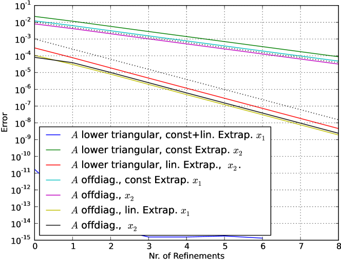
Figure 6 shows the convergence result for the four situations. To show the predictions made by (69) in terms of , it is necessary that the subsystems methods contribution is of higher order than the extrapolation and that the method used is a one-step method, which will be discussed in Section 4.2.3. Thus dopri5, an explicite Runge-Kutta method, was chosen, using the built-in stepsize control with default absolute tolerance .
The figure shows that convergence is of order 1 for constant extrapolation and of order 2 for linear extrapolation, as predicted by (69). As discussed, there is no order loss for linear extrapolation and circular dependency of inputs, but not even an higher error, in spite of the negative effects that should occur.
The error of the first component of the lower triangular, thus unidirectionally coupled system is very low as it has no extrapolation contribution, thus indicating that the error made by is low enough to allow for judgement of the effect of extrapolation error.
4.2.2 Spring-Mass system for convergence and stability
To numerically examine the stability of the method, we chose the linear spring-mass oscillator as discussed in [11] and given by
| (92) |
with mass , spring constant , and in which the damping constant shall vanish, for being simple while still showing stability problems. It is indeed a physical interpretation of the above system with offdiagonal matrix.
| Spring | Mass |
| System States | |
| Outputs | |
| Inputs | |
| Equations | |
| Spring | Mass |
| System States | |
| Outputs | |
| Inputs | |
| Equations | |
This system was treated in the cosimulation scheme 1.
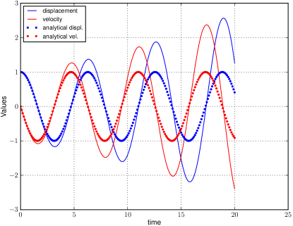
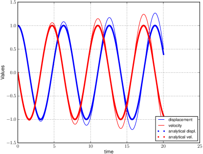
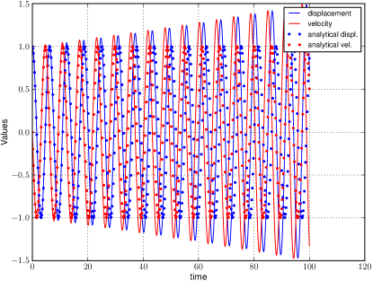
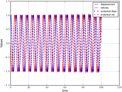
Output of the spring is the force , that of the mass is the velocity . As ODE solver on subsystems, any solver that does not dominate the convergence and stability behavior of the cosimulation scheme could be used. The plots 8 and 9 show simulations done with vode and zvode from the numpy Python numerics library, which both implement implicit Adams method if problem is nonstiff and BDF if it is and behave stable due to their step size adjustment. The convergence plot 7 was made with dopri5 (see Section 4.2.3).
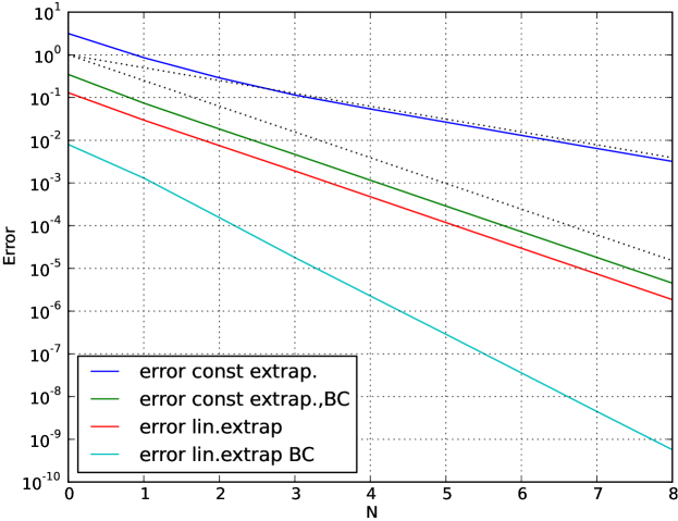
The numerical convergence examination backs up the results from section 3.4, estimate (69), and equation (88) – even more, balance corrected scheme for this problem converges of one order higher than proven there. A sharper theoretical result should be achievable.
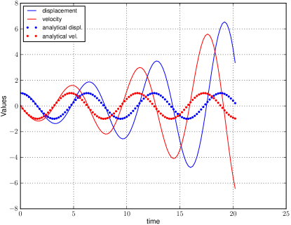
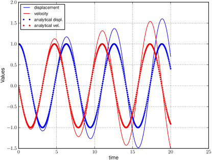
But the method is unstable for its explicite contributions, as proven in section 3.5. This means for . The energy of our system is , which is an equivalent norm, so lack of stability is equivalent to energy augmentation.
This lack of stability can be interpreted in physics as a consequence of extrapolation errors in factors of power acting on subsystems boundaries:
In [11] the problem arose
that errors in the force made during data exchange lead to errors in the power that acts on the mass. The system picks up energy and behaves unstable (See figure 8). This led to a reclassification to balance errors: Cumulated extrapolation errors in input variables that in fact are conserved quantities, and those in input variables that are factors of conserved quantities and such disturb a balance [11, Section 3.2].
4.2.3 Pitfall Subsystems methods
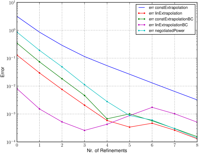
Multistep methods need additional initial values: an -step methods needs of them. Those initial values are usually calculated using one-step methods, possibly of lower order. Its error usually is not visible in the result, as it occurs only once in the calculation. But as subsystem solver restarts after data exchange, the error occurs times in cosimulation. Assume that the one-step method is of order . Then even if holds, sum of its error is . In figure 10, this is , as visible for the last two refinements. The local minimum in error is due to different signs of the two contributions and .
5 Discussion and Conclusion
By the estimates given in section 3.4, theorem 3.6 cosimulation methods are proven to be efficient methods, if the overall system is not too vulnerable to stability problems (see Section 3.5).
The stability issue will be tackled in a separate publication.
The convergence result is consistent with those in [2] and in [3], but include the error of the subsystems methods.
Moreover, with the provided methodology it can be proven that balance correction method converges at least with the same convergence order as the cosimulation scheme without balance correction, see theorem 4.1 from section 4. For most problems it should be the case that convergence order rises by one if balance correction is applied, as the test problems and superficial considerations indicate.
Finding a sharper theoretical result for balance correction techniques seems a realistic future task.
References
- [1] Martin Arnold, Constanze Bausch, Torsten Blochwitz, Christoph Clau , Manuel Monteiro, Thomas Neidhold, J rg-Volker Peetz and Susann Wolf, Functional Mock-up Interface for Co-Simulation, 2010.
- [2] Martin Arnold, Christoph Clauss and Tom Schierz, Error Analysis and Error Estimates for Co-Simulation in FMI for Model Exchange and Co-Simulation V2.0, 60.1 (2013), 75–94.
- [3] Martin Arnold and Michael Günther, Preconditioned Dynamic Iteration for Coupled Differential-Algebraic Systems, BIT Numerical Mathematics 41 (2001), 1–25 (English).
- [4] M. Busch, Zur effizienten Kopplung von Simulationsprogrammen, Ph.D. thesis, 2012.
- [5] Peter Deuflhard and Folkmar A. Bornemann, Numerische Mathematik II, de Gruyter, 1994.
- [6] Sicklinger; Belsky; Engelmann; Elmqvist, Interface Jacobian-based Co-Simulation, International Journal for Numerical Methods in Engineering 98 (2014), 418–444.
- [7] Roland Kossel, Hybride Simulation thermischer Systeme am Beispiel eines Reisebusses, Ph.D. thesis, Braunschweig, Techn. Univ., 2012, p. 112.
- [8] R. Kübler and W. Schiehlen, Modular Simulation in Multibody System Dynamics, Multibody System Dynamics 4 (2000), 107–127.
- [9] Ulla Miekkala and Olavi Nevanlinna, Convergence of Dynamic Iteration Methods for Initial Value Problems, SIAM J. Sci. and Stat. Comput 8 (1987), 459–482.
- [10] Dirk Scharff, Christian Kaiser, Wilhelm Tegethoff and Michaela Huhn, Ein einfaches Verfahren zur Bilanzkorrektur in Kosimulationsumgebungen, in: SIMVEC - Berechnung, Simulation und - Erprobung im Fahrzeugbau, 2012.
- [11] Dirk Scharff, Thilo Moshagen and Jaroslav Vondřejc, Treating Smoothness and Balance during Data Exchange in Explicit Simulator Coupling or Cosimulation, (2017), 30.
- [12] M.; Wells, J.; Hasan and C. Lucas, Predictive Hold with Error Correction Techniques that Maintain Signal Continuity in Co-Simulation Environments, SAE Int. J. Aerosp (2012), 481–493.