Analyzing Large-Scale Multiuser Molecular Communication via 3D Stochastic Geometry

Abstract

Information delivery using chemical molecules is an integral part of biology at multiple distance scales and has attracted recent interest in bioengineering and communication theory. Potential applications include cooperative networks with a large number of simple devices that could be randomly located (e.g., due to mobility). This paper presents the first tractable analytical model for the collective signal strength due to randomly-placed transmitters in a three-dimensional (3D) large-scale molecular communication system, either with or without degradation in the propagation environment. Transmitter locations in an unbounded and homogeneous fluid are modelled as a homogeneous Poisson point process. By applying stochastic geometry, analytical expressions are derived for the expected number of molecules absorbed by a fully-absorbing receiver or observed by a passive receiver. The bit error probability is derived under ON/OFF keying and either a constant or adaptive decision threshold. Results reveal that the combined signal strength increases proportionately with the transmitter density, and the minimum bit error probability can be improved by introducing molecule degradation. Furthermore, the analysis of the system can be generalized to other receiver designs and other performance characteristics in large-scale molecular communication systems.

I Introduction

Molecular communication via diffusion has attracted significant bioengineering and communication engineering research interest in recent years [2]. Messages are delivered via molecules undergoing random walks [3], which is a prevalent phenomenon in biological systems and between organisms [4] across multiple distance scales, offering transmit energy and signal propagation advantages over wave-based communications [5, 6, 7]. More importantly, when compared to electromagnetic wave-based communication systems, molecular communication can be advantageous at very small dimensions or in specific environments, such as in salt water or human bodies.

Fundamentally, molecular communications involves modulating information on the physical properties (e.g., number, type, emission time) of a single molecule or group of molecules (such as pheromones, DNA, protein). When modulating the number of molecules, each messenger node will transmit information-bearing molecules via chemical pulses. According to the theory of Brownian motion, the average displacement of each molecule is proportional to its diffusion time and the diffusion coefficient, however, the instantaneous displacement of each molecule differs and is usually described by the Normal distribution [8]. As such, a molecule emitted in a previous bit interval may arrive at the receiver during the current interval, thereby confusing the signal detection at the receiver with intersymbol interference (ISI).

Existing works have largely focused on modeling the signal strength of a point-to-point communication channel by taking into account the self-interference that arises from previous symbols (i.e., ISI) at a passive receiver [9], at a fully absorbing receiver [10], and at a reversible adsorption receiver [11]. Efforts to mitigate ISI include transmitting using two different types of molecules in consecutive bit intervals [12], and designing ISI-free codes [13].

Recent advances in bio-nanotechnology bring new opportunities for enabling molecular communication in new applications, such as drug delivery, environmental monitoring, and pollution control. One application example is that swarms of nano-robots could track specific targets, such as tumour cells, to perform operations such as targeted drug delivery [14]. In such a scenario, each nano-robot may receive the signal transmitted from multiple nano-robots. Thus, how to establish energy efficient and tether-less communication becomes an important research problem [15].

In nanonetworks, it is therefore important to provide a physical model for the collective signal strength at the receiver in a large-scale system, while taking into account random transmitter locations due to mobility. In [16], the collective signal strength of a multi-access communication channel at a passive receiver due to co-channel transmitters (i.e., transmitters emitting the same type of molecule) was measured given the knowledge of their total number and locations. In [17], the capacity of the multiple access channel with a single bit emitted at each transmitter and a ligand-binding receiver was derived under the assumption of a deterministic diffusion channel model. The first work to consider randomly distributed co-channel transmitters in a 3D diffusion channel according to a spatial homogeneous Poisson point process (HPPP) is [18], where the probability density function (PDF) of the received power spectral density at a point receiver was derived based on the assumption of white Gaussian transmit signals. The analysis in [18] considers multiuser emission within a single transmission interval, and the presented results are Monte Carlo simulations.

From the perspective of receiver design, many works have focused on the passive receiver, which can observe and count the number of molecules inside the receiver without interfering with the molecules [9, 16, 18]. In nature, receivers commonly remove information molecules from the environment once they bind to a receptor. An ideal model is the fully absorbing receiver, which absorbs all the molecules hitting its surface [10, 11]. Unfortunately, no work has studied the channel characteristics and the received signal at a fully absorbing receiver in a large-scale molecular communication system, nor compared it with that at a passive receiver.

In this paper, we aim to provide an analytical model and bit error probability for the collective signal at the passive receiver and the fully absorbing receiver due to a swarm of active mobile point transmitters that simultaneously emit the same bit sequence. We extend our previous work in [1] by deriving the bit error probability of a constant threshold detector at both receivers under fixed threshold-based demodulation, and applying decision feedback detection (DFD) for performance improvement. Our new analysis takes into account the molecule degradation during diffusion based on the following three facts: 1) molecules are unlikely to persist for all time, and may be degraded by chemical reactions in a biological environment; 2) the constant transmitter density over unbounded space assumed in our analytical model implies that there is an infinite number of transmitters and that ISI increasingly accumulates, which isn’t practical; 3) the molecule degradation will help to reduce the ISI and improve the probability of error.

The analytical results are obtained via the powerful tools of stochastic geometry in 3D space, which can characterize the average behavior over many spatial realizations of a network where the transmitter nodes are placed according to some probability distribution [19]. Just as we can analyze the network performance of a random field of transmitters in conventional wireless networks, we can also apply a similar rationale for analyzing the receiver performance due to a swarm of molecular transceivers. However, unlike [20, 21], where the network performance is analyzed based on the distribution of the received signal-to-interference-plus-noise ratio (SINR) at a point receiver in 2D space, we seek the mean and distribution of the number of received molecules at a spherical receiver due to all transmitters in 3D space. By doing so, simple and tractable results can be obtained to reveal the key dependency of the molecular communication system performance metrics with respect to the system parameters. This work and [1] are distinct from related work in [18], which focused on the statistics of the received signal at any point location. Our contributions can be summarized as follows:

1. Using stochastic geometry, we model the collective signal at a receiver in a 3D large-scale molecular communication system with or without molecule degradation, where the receiver is either passive or fully absorbing. To examine the impact of the signal from the nearest transmitter relative to the aggregate signal, we also derive the signals from the nearest transmitter and the other transmitters.

2. We derive a general expression for the expected net number of molecules observed at both types of receivers during any time interval. In order to gain insights about the impact of the transmitter density, the diffusion coefficient, and the receiver radius on the collective signal, we simplify the general expression to a closed-form expression for the expected net number of molecules absorbed at the fully absorbing receiver under molecule degradation.

3. We derive a general expression for the bit error probability at the passive or absorbing receiver in the proposed system with or without molecule degradation under ON/OFF keying. A simple detector requiring one sample per bit interval is considered as a preliminary design for the proposed large-scale system. Importantly, this general expression for the bit error probability can also be applied for other types of receivers by substituting the corresponding channel response.

4. We focus on Monte Carlo simulation approaches to verify our analytical results, and we also compare Monte Carlo simulation to particle-based simulation of the large-scale molecular communication system. It is shown that the expected number of molecules observed at both types of receivers increases linearly with increasing transmitter density. We also show that the minimum bit error probability of both receivers can be improved by introducing molecule degradation.

The rest of this paper is organized as follows. In Section II, we introduce the system model. In Section III, we present the channel impulse response of information molecules in the large-scale molecular communication system. In Section IV, we derive the exact and asymptotic net number of absorbed molecules expected at the surface of the absorbing receiver, and the exact number of molecules observed inside the passive receiver in the large-scale molecular communication system. In Section V, we derive the bit error probability of the proposed system with a simple detector requiring one sample per bit. In Section VI, we present the numerical and simulation results. In Section VII, we conclude the contributions of this paper.

II System Model

In Fig. 1, we consider a 3D diffusion-based molecular communication system with a single receiver located at the origin under joint transmission by a swarm of point transmitters, which are spatially distributed outside the receiver in $\mathbb{R}^{3}/{V_{{\Omega_{{r_{r}}}}}}$ according to an independent and homogeneous Poisson point process (HPPP) $\Phi_{a}$ with density $\lambda_{a}$, where ${V_{{\Omega_{{r_{r}}}}}}$ is the volume of receiver ${{\Omega_{{r_{r}}}}}$ with ${V_{{\Omega_{{r_{r}}}}}}={{4\pi r_{r}^{3}}\mathord{\left/{\vphantom{{4\pi r_{r}^{3}}3}}\right.\kern-1.2pt}3}$. HPPP has been widely used to model wireless sensor networks [20, 22], homogeneous and heterogeneous cellular networks [19, 23], and has also been applied to model bacterial colonies in [24] and the interference sources in a molecular communication system [18]. We note that we focus on an unbounded fluid environment with uniform diffusion and no flow currents to provide a baseline for the design of more complicated scenarios in future works.

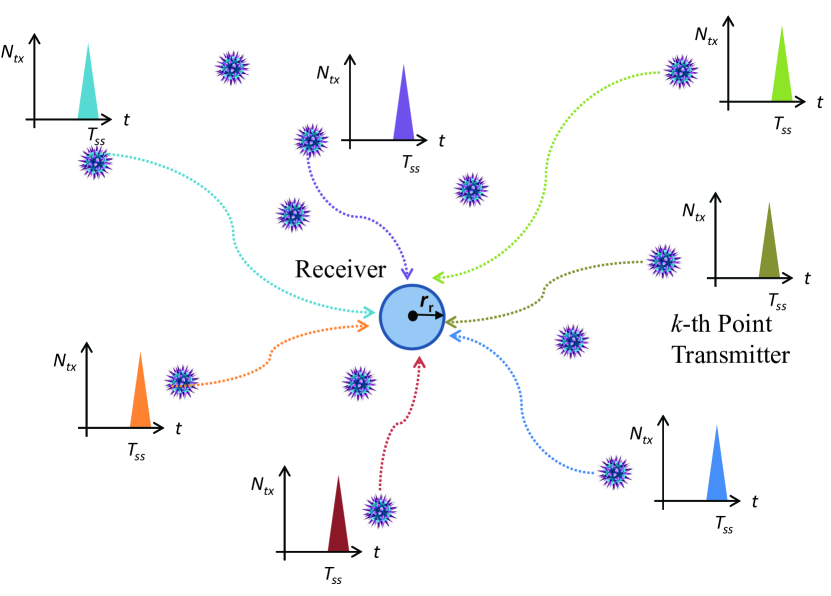
Figure 1: Illustration of a receiver receiving molecular pulse signals from point transmitters at different distances.

We consider a spherical receiver that is either passive [6, 25] or fully absorbing [26]. The fully absorbing receiver is covered with selective independent receptors, which are only sensitive to a single type of information molecule. Similar to [26, 11], we assume that there is no physical limitation on the number of receptors on the surface of the receiver, which is an appropriate assumption for a system with a sufficiently large number of receptors or small number of absorbed molecules. Any information molecule that diffuses into the sphere is absorbed by a receptor and counted for information demodulation. The passive receiver is covered with a transparent membrane that is permeable to the information molecules passing by, and the number of information molecules inside the receiver can be counted for information demodulation as in [16].

Even though this work considers a molecular communication system with a single receiver, it provides fundamental insights that can be applied to consider systems with multiple transceivers in future work. For example, in the case of multiple passive receivers following HPPP, the expected number of molecules inside any passive receiver with the same radius will be equivalent due to the Slivnyak-Mecke’s theorem [27]. In other words, the presence of multiple passive receivers will not influence the observations at each passive receiver, due to its transparent membrane. This is also consistent with the stochastic geometry work on cellular networks, where the average ergodic rate of an arbitrary random mobile user is expressed using a single expression [21]. However, for the case of multiple absorbing receivers, the numbers of molecules absorbed by each absorbing receiver is not independent; in other words, the presence or absence of an absorbing receiver influences the numbers of molecules absorbed by other absorbing receivers. For a system of absorbing receivers, the average observation will be harder to characterize, but understanding the single receiver system is still the first step.

A molecular communication system typically includes five processes: emission, propagation, reception, modulation, and demodulation, which are presented in detail in the following subsections for the absorbing receiver and the passive receiver, respectively.

II-A Emission $\&$ Modulation

Applying ON/OFF keying as in [26, 11], each transmitter delivers molecular signal pulses with $N_{\rm{tx}}$ type $S$ information molecules to the receiver at the start of each bit interval to represent transmit bit-1, and emits zero molecules to deliver bit-0. Here, a global clock is assumed at each transmitter such that the molecule emissions at all the transmitters are synchronized with the same bit sequences, and can only occur at the start of a bit interval as in [18]. Asynchronous emission can be evaluated similarly to synchronous emission by allowing transmitters to release molecules at the start of intervals that are much smaller than the bit interval, and scaling the transmitter density accordingly.

II-A1 Absorbing Receiver

In the absorbing receiver scenario, we assume spherical symmetry, where the transmitter is effectively a point on the spherical shell with radius $r_{0}$ away from the center of receiver and the molecules are released from random points over the shell at $t=0$; the actual angle to the transmitter when a molecule hits the receiver is irrelevant. Thus, we define the initial condition as [28, Eq. (3.61)]

$$C^{\text{FA}}\left({r,\left.{t\to 0}\right|{r_{0}}}\right)=\frac{1}{{4\pi{r_{0}}^{2}}}\delta\left({r-{r_{0}}}\right),$$ (1)

where $C^{\text{FA}}\left({r,\left.{t\to 0}\right|{r_{0}}}\right)$ is the molecule distribution function at time ${t\to 0}$ and distance $r$ with initial distance $r_{0}$ .

According to (1), there is spherical symmetry that makes the molecules initially distributed with equal probability over a spherical surface at distance $r_{0}$ from the receiver. Mathematically, Eq. (1) represents the impulse response averaged over the surface area of the ball, where ${4\pi{r_{0}}^{2}}$ is the surface area of the ball centered at the center of receiver. The direct interpretation is that, due to spherical symmetry, a shell transmitter is analogous to a point transmitter. As an example, consider an absorbing receiver and two molecules that are initially placed at two points equidistant from the receiver. Each molecule has the same probabilistic trajectory for hitting the receiver. Since they are equidistant from the receiver, we can merge them to a single point source to achieve the same result.

II-A2 Passive receiver

In the passive receiver scenario, we assume an asymmetric spherical model, which accounts for the actual angle of the molecule inside the passive receiver. The information particles are injected into the fluid environment by a transmitter located at ${\overrightarrow{r}}$ away from the center of the passive receiver [8].

II-B Diffusion Under Molecule Degradation

The diffusion of molecules in the propagation process follows random Brownian motion. With a sufficiently low concentration of information molecules in the fluid environment, the collisions between these molecules can be ignored and the molecules propagate independently with constant diffusion coefficient $D$ . This concentration changes over time due to diffusion as described by Fick’s second law, and determines the spatial and temporal variation of non-uniform distributions of particles [8, Ch.2].

To reduce the ISI, we introduce molecule degradation that can occur at any time via a chemical reaction mechanism in the form of [25, 30, 31]

$$S\mathop{\to}\limits^{{k_{d}}}P,$$ (2)

where $k_{d}$ is the degradation rate in $\text{s}^{-1}$, and $P$ is another type of molecule that cannot be recognized by either type of receiver. The degradation rate $k_{d}$ relates to the half-life (${{\Lambda_{{1\mathord{\left/{\vphantom{12}}\right.\kern-1.2pt}2}}}}$) of messenger molecules via $k_{d}=\frac{{\ln 2}}{{{\Lambda_{{1\mathord{\left/{\vphantom{12}}\right.\kern-1.2pt}2}}}}}$, and $k_{d}=0$ corresponds to the no degradation case.

II-C Reception

II-C1 Absorbing Receiver

Any information molecules that hit the absorbing receiver will be captured for information demodulation. This reception process at the fully absorbing receiver can be described as [28, Eq. (3.64)]

$${\left.{D\frac{{\partial\left({C^{\text{FA}}\left({r,\left.t\right|{r_{0}}}\right)}\right)}}{{\partial r}}}\right|_{r=r_{r}^{+}}}={k}C^{\text{FA}}\left({{r_{r}},\left.t\right|{r_{0}}}\right),k\to\infty$$ (3)

where $k$ is the absorption rate (in length$\times$time^-1).

II-C2 Passive receiver

With a transparent membrane at the passive receiver, the information molecules can bypass the surface of the passive receiver freely, and molecules within the receiver can be counted at any time [8].

II-D Demodulation

For equivalent comparison, the number of molecules absorbed by the surface of the absorbing receiver and the number of observed molecules inside the passive receiver at the end of each bit interval are collected for information demodulation. More details of the demodulation at each type of receiver are described as follows.

II-D1 Demodulation criterion at the absorbing receiver

With spherical symmetry, we only need to focus on the number of molecules absorbed by the surface of the receiver $r=r_{r}$. We consider an absorbing receiver that is capable of counting the net number of molecules absorbed by the surface of the receiver as in [11] by subtracting the number of absorbed molecules at the end of the previous bit interval from that at the end of the current bit interval. The net number of molecules absorbed over the $j$th bit interval ${N_{\rm{net}}^{\rm{FA}}\left[j\right]}$ is demodulated as the received signal of the $j$th bit (${N^{\rm{Rx}}\left[j\right]}={N_{\rm{net}}^{\rm{FA}}\left[j\right]}$). This is because for the single bit transmission at $t=0$, as time increases, the number of absorbed molecules increases, which results in increasing ISI, whereas the average net number of absorbed molecules in a given bit interval $T_{b}$ becomes a constant value as $T_{b}$ goes to infinity in a large-scale molecular communication system as shown in Section IV.

II-D2 Demodulation criterion at the passive receiver

With a transparent membrane, the passive receiver is assumed to be capable of counting the number of molecules currently inside the passive receiver at the end of the $j$th bit interval ${N_{\rm{cur}}^{\rm{PA}}\left[j\right]}$ for information demodulation (${N^{\rm{Rx}}\left[j\right]}={N_{\rm{cur}}^{\rm{PA}}\left[j\right]}$). This is because the current number of observed molecules inside the receiver can remain at a comparable value for a long time in the large-scale molecular communication system as will be shown in Fig. 3 in Section VI. For this reason, we only use a simple detector design with one sample collected at the end of each bit interval rather than multiple samples in each bit interval.

II-D3 Demodulation schemes at both receivers

We first consider a fixed threshold-based demodulation with the same decision threshold $N_{\rm{th}}$ for all bits at both types of receivers, where the receiver demodulates the received signal as bit-1 if ${N^{\rm{Rx}}\left[j\right]}\geq N_{\rm{th}}$, and demodulates the received signal as bit-0 if ${N^{\rm{Rx}}\left[j\right]}<N_{\rm{th}}$. In the fixed threshold-based demodulation, the received molecules ${N^{\rm{Rx}}\left[j\right]}$ will accumulate as more bits are transmitted and molecules arrive from more distant transmitters, and inevitably impair the system reliability as ISI.

To remove this accumulation, we then consider the demodulation scheme using a DFD [32] with the decision threshold $N_{\rm{th}}$ at both types of receivers in Section VI, based on the subtraction between ${N^{\rm{Rx}}}$ in the current bit and that in the previous bit. More specifically, the receiver demodulates the received signal as bit-1 if $\{{N^{\rm{Rx}}\left[j\right]}-{N^{\rm{Rx}}\left[j-1\right]}\}\geq N_{\rm{th}}$, and demodulates the received signal as bit-0 if $\{{N^{\rm{Rx}}\left[j\right]}-{N^{\rm{Rx}}\left[j-1\right]}\}<N_{\rm{th}}$.

III Channel Impulse Response

In this section, we present the channel impulse responses at the absorbing receiver and at the passive receiver in the large-scale molecular communication system due to the single bit-1 transmission at each point transmitter.

III-A Absorbing Receiver

III-A1 Point-to-point system

We first provide the background for the receiver observation of a single point transmitter located distance $r_{0}$ away from the center of the absorbing receiver. To do so, we calculate the rate of absorption at the surface of the absorbing receiver due to the transmitter at distance $r_{0}$ via [28, Eq. (3.106)]

$$K\left({\left.t\right|{r_{0}}}\right)=4\pi r_{r}^{2}D{\left.{\frac{{\partial C^{\text{FA}}\left({\left.{r,t}\right|{r_{0}}}\right)}}{{\partial r}}}\right|_{r={r_{r}}}},$$ (4)

where the molecule distribution function

$$C^{\text{FA}}\left({\left.{r,t}\right|{r_{0}}}\right)=\frac{1}{{4\pi r{r_{0}}}}\frac{1}{{\sqrt{4\pi Dt}}}\left({{e^{-\frac{{{{\left({r-{r_{0}}}\right)}^{2}}}}{{4Dt}}}}-{e^{-\frac{{{{\left({r+{r_{0}}-2{r_{r}}}\right)}^{2}}}}{{4Dt}}}}}\right),$$ (5)

is derived in [28].

Substituting (5) into (4), the first hitting probability is derived as

$$K\left({\left.t\right|{r_{0}}}\right)=\frac{{{r_{r}}}}{{{r_{0}}}}\frac{1}{{\sqrt{4\pi D{t}}}}\frac{{{r_{0}}-{r_{r}}}}{t}{e^{-\frac{{{{\left({{r_{0}}-{r_{r}}}\right)}^{2}}}}{{4Dt}}}}.$$ (6)

Taking into account molecule degradation, the fraction of molecules absorbed by the receiver due to a transmitter at distance $r_{0}$ during any sampling interval $[t,t+T_{ss}]$ with a single impulse pulse occurring at $t=0$ reduces to

$$F^{{\rm{FA}}} \left({\left.{{\Omega_{{r_{r}}}},t,t+{T_{ss}}}\right|{r_{0}}}\right)$$

$$=F^{{\rm{FA}}}\left({\left.{{\Omega_{{r_{r}}}},0,t+{T_{ss}}}\right|{r_{0}}}\right)-F^{{\rm{FA}}}\left({\left.{{\Omega_{{r_{r}}}},0,t}\right|{r_{0}}}\right),$$ (7)

where

$${{F^{\rm{FA}}}\left({\left.{{\Omega_{{r_{r}}}},0,t}\right|{r_{0}}}\right)} =\int_{0}^{t}{K\left({\left.t\right|{r_{0}}}\right){e^{-{k_{d}}t}}dt}$$

$$=\frac{{{r_{r}}}}{{{r_{0}}}}\exp\left({-\sqrt{\frac{{k_{d}}}{D}}\left({{r_{0}}-{r_{r}}}\right)}\right)-\frac{{{r_{r}}}}{{2{r_{0}}}}{\exp\left(-\sqrt{\frac{{k_{d}}}{D}}\left({{r_{0}}-{r_{r}}}\right)\right)}$$

$$\left[{\operatorname{erf}\left({\frac{{{r_{0}}-{r_{r}}}}{{\sqrt{4Dt}}}-\sqrt{k_{d}}t}\right)+{\exp\left({2\sqrt{\frac{{k_{d}}}{D}}\left({{r_{0}}-{r_{r}}}\right)}\right)}}\right.$$

$$\left.{\left({\operatorname{erf}\left({\frac{{{r_{0}}-{r_{r}}}}{{\sqrt{4Dt}}}+\sqrt{k_{d}}t}\right)-1}\right)+1}\right].$$ (8)

We note that (8) is derived following the method for the point-to-point system in [30, Eq. (12)]. We see that increasing $k_{d}$ decreases the fraction of molecules absorbed by the absorbing receiver.

Without molecule degradation ($k_{d}=0$), ${{F^{\rm{FA}}}\left({\left.{{\Omega_{{r_{r}}}},0,t}\right|{r_{0}}}\right)}$ simplifies to [26, Eq. (32)]

$${{F^{\rm{FA}}}\left({\left.{{\Omega_{{r_{r}}}},0,t}\right|{r_{0}}}\right)} =\frac{{{r_{r}}}}{{r_{0}}}\operatorname{erfc}\Big{\{}{\frac{{r_{0}-{r_{r}}}}{{\sqrt{4D{t}}}}}\Big{\}}.$$ (9)

III-A2 Large-scale system

In our proposed large-scale system, the center of an absorbing receiver is fixed at the origin of a 3D fluid environment.

Using the Slivnyak-Mecke’s theorem [27], the fraction of absorbed molecules at the receiver during any sampling interval $[t,t+T_{ss}]$ due to an arbitrary point transmitter $x$ at the location x emitting a single pulse at $t=0$ ${{F^{\rm{FA}}}\left({\left.{{\Omega_{{r_{r}}}},t,t+T_{ss}}\right|{\left\|\textbf{x}\right\|}}\right)}$ can be obtained via (8), where $\left\|\textbf{x}\right\|$ is the distance between the point transmitter and the center of the receiver where the transmitters follow a HPPP.

Recalling that the propagation of each molecule is independent, the cumulative fraction $F^{\rm{FA}}_{\rm{all}}$ of absorbed molecules at the receiver during any sampling interval $[t,t+T_{ss}]$ due to all active point transmitters emitting a single pulse at $t=0$ can be formulated as

$${{F_{\rm{all}}^{{\rm{FA}}}}\left({{{\Omega_{{r_{r}}}},t,t+T_{ss}}}\right)}=\sum\limits_{x\in{\Phi_{a}}}{{F^{\rm{FA}}}\left({\left.{{\Omega_{{r_{r}}}},t,t+T_{ss}}\right|{\left\|\textbf{x}\right\|}}\right)},$$ (10)

where ${{F^{\rm{FA}}}\left({\left.{{\Omega_{{r_{r}}}},t,t+T_{ss}}\right|{\left\|\textbf{x}\right\|}}\right)}$ can be obtained from (8).

The expected net number of molecules absorbed by the receiver during any sampling interval $[t,t+T_{ss}]$ due to all of the active point transmitters emitting a single pulse at $t=0$ can be calculated as

$${\mathbb{E}}\left\{{N_{{\rm{all}}}^{{\rm{FA}}}\left({{{\Omega_{{r_{r}}}},t,t+T_{ss}}}\right)}\right\} ={N_{\rm{tx}}}{\mathbb{E}}\Big{\{}{F_{\rm{all}}^{{\rm{FA}}}\left({{{\Omega_{{r_{r}}}},t,t+T_{ss}}}\right)}\Big{\}},$$ (11)

where $N_{{\rm{all}}}^{{\rm{FA}}}\left({{{\Omega_{{r_{r}}}},t,t+T_{ss}}}\right)$ is the net number of absorbed molecules, and ${F_{\rm{all}}^{{\rm{FA}}}\left({{{\Omega_{{r_{r}}}},t,t+T_{ss}}}\right)}$ is given in (10).

It is well known that the distance between the transmitter and the receiver in molecular communication is the main contributor to the signal strength. In the absence of flow, the nearest transmitter will provide the strongest signal for the receiver. In order to examine the impact of the signal from the nearest transmitter on the received signal in the large-scale molecular communication system, we present the expected number of absorbed molecules at this receiver during any sampling interval $[t,t+T_{ss}]$ due to a single pulse emission by the nearest transmitter as

$${{\mathbb{E}}_{\rm{u}}^{{\rm{FA}}}}={\mathbb{E}}\Big{\{}{{F^{\rm{FA}}}\left({\left.{{\Omega_{{r_{r}}}},t,t+T_{ss}}\right|{\left\|\textbf{x}^{*}\right\|}}\right)}\Big{\}},$$ (12)

where $\left\|\textbf{x}^{*}\right\|$ denotes the distance between the receiver and the nearest transmitter,

$$\quad x^{*}=\mathop{\arg\min}\limits_{x\in{\Phi_{a}}}\left\|{{\textbf{x}}}\right\|,$$ (13)

$x^{*}$ denotes the nearest point transmitter for the receiver, and ${\Phi_{a}}$ denotes the set of active transmitters’ positions.

To examine the impact of the aggregate signal from the remaining transmitters, we present the expected number of absorbed molecules at this receiver during any sampling interval $[t,t+T_{ss}]$ due to single pulse emissions by the other transmitters as

$${{\mathbb{E}}_{\rm{o}}^{{\rm{FA}}}}={\mathbb{E}}\Bigg{\{}\sum\limits_{{{x\in{\Phi_{a}}}\mathord{\left/{\vphantom{{{\Phi_{a}}}{{{x}^{*}}}}}\right.\kern-1.2pt}{{{x}^{*}}}}}{{F^{\rm{FA}}}\left({\left.{{\Omega_{{r_{r}}}},t,t+T_{ss}}\right|{\left\|\textbf{x}\right\|}}\right)}\Bigg{\}},$$ (14)

where ${{F^{\rm{FA}}}\left({\left.{{\Omega_{{r_{r}}}},t,t+T_{ss}}\right|{\left\|\textbf{x}\right\|}}\right)}$ is given in (8).

III-B Passive Receiver

III-B1 Point-to-point system

In a point-to-point molecular communication system with a single point transmitter located at ${\overrightarrow{r}}$ relative to the center of a passive receiver with radius $r_{r}$, the local point concentration at the center of the passive receiver at time $t$ due to a single pulse emission by the transmitter occurring at $t=0$ is given as [33, Eq. (4.28)]

$$C\left({\left.{{{{\Omega}}_{{r_{r}}}},t}\right|{\overrightarrow{r}}}\right)=\frac{1}{{{{\left({4\pi Dt}\right)}^{{3\mathord{\left/{\vphantom{32}}\right.\kern-1.2pt}2}}}}}\exp\Big{(}{-\frac{{{{\left|{\overrightarrow{r}}\right|}^{2}}}}{{4Dt}}}\Big{)},$$ (15)

where $\overrightarrow{r}=[x,y,z]$, and $[x,y,z]$ are the coordinates along the three axes.

The fraction of molecules observed inside the passive receiver with volume ${V_{{\Omega_{{r_{r}}}}}}$ at time $t$ is denoted as

$${F^{\rm{PS}}}\left({\left.{{\Omega_{{r_{r}}}},t}\right|{\left|{\overrightarrow{r}}\right|}}\right) =\int\limits_{{{{\Omega_{{r_{r}}}}}}}{C\left({\left.{{{\Omega}_{{r_{r}}}},t}\right|{\overrightarrow{r}}}\right)\mathop{}\!\mathrm{d}{{{{\Omega_{{r_{r}}}}}}}}.$$ (16)

In most molecular communication literature considering a passive receiver, the uniform concentration assumption inside the passive receiver is applied, which immediately results in the fraction of observed molecules inside the passive receiver as

$${F^{\rm{PS}}}\left({\left.{{\Omega_{{r_{r}}}},t}\right|{\left|{\overrightarrow{r}}\right|)}}\right) \approx{C\left({\left.{{{\Omega}_{{r_{r}}}},t}\right|\left|{\overrightarrow{r}}\right|}\right){{V_{{\Omega_{{r_{r}}}}}}}},$$ (17)

however, this result relies on the receiver being sufficiently far from the transmitter (see [34]), which we cannot guarantee here since the transmitters are placed randomly.

With the actual non-uniform concentration inside the passive receiver, the fraction of observed molecules inside the passive receiver is calculated as

$${F^{{\rm{PS}}}}\left({\left.{{\Omega_{{r_{r}}}},t}\right|\left|{\overrightarrow{r}}\right|}\right){\rm{}}=\int\limits_{0}^{{r_{r}}}{\int\limits_{0}^{2\pi}{\int\limits_{0}^{\pi}{C\left({\left.{{{\Omega}_{{r_{r}}}},t}\right|{\overrightarrow{r}}}\right)r^{2}\sin\theta}}}\mathop{}\!\mathrm{d}\theta\mathop{}\!\mathrm{d}\phi\mathop{}\!\mathrm{d}r.$$ (18)

The molecule degradation introduces a decaying exponential term as in [25, Eq. (10)]. Therefore, according to (18) and Theorem 2 in [34], the fraction ${F^{\rm{PS}}}$ of molecules observed inside the passive receiver at time $t$ due to a single pulse emission by a transmitter at $r_{0}$ away from the center of a passive receiver with radius $r_{r}$ at time $t=0$ is derived as

$${F^{\rm{PS}}}\left({\left.{{\Omega_{{r_{r}}}},t}\right|{r_{0}}}\right)={e^{-{k_{d}}t}}\Bigg{[}\frac{1}{2}\Big{[}{{\rm{erf}}\Big{(}{\frac{{{r_{r}}-{r_{0}}}}{{2\sqrt{Dt}}}}\Big{)}+{\rm{erf}}\Big{(}{\frac{{{r_{r}}+{r_{0}}}}{{2\sqrt{Dt}}}}\Big{)}}\Big{]}\Bigg{.}$$

$$\Bigg{.}+{\frac{{\sqrt{Dt}}}{\sqrt{\pi}{{r_{0}}}}}\Big{[}{\exp\Big{(}{-\frac{{{{\left({{r_{r}}+{r_{0}}}\right)}^{2}}}}{{4Dt}}}\Big{)}-\exp\Big{(}{-\frac{{{{\left({{r_{0}}-{r_{r}}}\right)}^{2}}}}{{4Dt}}}\Big{)}}\Big{]}\Bigg{]}.$$ (19)

We see from (19) that increasing $k_{d}$ decreases the fraction of molecules observed at the passive receiver.

III-B2 Large-scale system

In the large-scale molecular communication system with a passive receiver centered at the origin, the fraction $F^{\rm{PS}}$ of molecules observed inside the passive receiver at time $T_{ss}$ due to an arbitrary point transmitter $x$ at the location x emitting a single pulse at $t=0$, ${{F^{\rm{PS}}}\left({\left.{{\Omega_{{r_{r}}}},t}\right|{\left\|\textbf{x}\right\|}}\right)}$ can be obtained using (19).

Due to the independent propagation of each molecule, the expected number of molecules observed inside the receiver at time $T_{ss}$ due to a single pulse emission by all transmitters at $t=0$ is given as

$${\mathbb{E}}\left\{{N_{\rm{all}}^{{\rm{PS}}}\left({{{\Omega_{{r_{r}}}},T_{ss}}}\right)}\right\}= \underbrace{N_{{\rm{tx}}}{\mathbb{E}}\Big{\{}{F^{{\rm{PS}}}}\left({\left.{{\Omega_{{r_{r}}}},T_{ss}}\right|\left\|{{{\bf{x}}^{*}}}\right\|}\right)\Big{\}}}_{{\mathbb{E}}_{\rm{u}}^{{\rm{PS}}}}$$

$$+\underbrace{{N_{\rm{tx}}}{\mathbb{E}}\Bigg{\{}{\sum_{x\in{{{\Phi_{a}}}\mathord{\left/{\vphantom{{{\Phi_{a}}}{{x^{*}}}}}\right.\kern-1.2pt}{{x^{*}}}}}}{F^{{\rm{PS}}}}\left({\left.{{\Omega_{{r_{r}}}},T_{ss}}\right|\left\|{\bf{x}}\right\|}\right)\Bigg{\}}}_{{\mathbb{E}}_{\rm{o}}^{{\rm{PS}}}},$$ (20)

where ${{F^{\rm{PS}}}\left({\left.{{\Omega_{{r_{r}}}},T_{ss}}\right|{\left\|\textbf{x}\right\|}}\right)}$ is obtained using (19), ${{\mathbb{E}}_{\rm{u}}^{{\rm{PS}}}}$ is the expected number of molecules observed inside the receiver at time $T_{ss}$ due to the nearest transmitter, and ${{\mathbb{E}}_{\rm{o}}^{{\rm{PS}}}}$ is the expected number of molecules observed inside the receiver at time $T_{ss}$ due to the other transmitters.

IV Receiver Observations

In this section, we first derive the distance distribution between the receiver and the nearest point transmitter. Throughout this section, we focus on the receiver observations at the receivers due to a single emission at each point transmitter at $t=0$. To understand the impact of individual TXs relative to the aggregate signal, we derive exact expressions for the expected number of molecules observed at the receiver due to the nearest point transmitter and that due to the other transmitters. We then present exact expressions for the expected number of molecules observed at the receiver due to all transmitters.

IV-A Distance Distribution

Unlike the stochastic geometry modelling of wireless networks, where the transmitters are randomly located in unbounded space, we impose that the point transmitters in a molecular communication system can only be distributed outside the surface of the spherical receiver. Taking into account the minimum distance $r_{r}$ between point transmitters and the receiver center, we derive the PDF of the shortest distance between a point transmitter and the receiver with radius $r_{r}$ in the following proposition.

Proposition 1.

The PDF of the shortest distance between any point transmitter and the receiver with radius $r_{r}$ in 3D space is

$${f_{\left\|{{\bf{x}^{*}}}\right\|}}(x)=4\lambda_{a}\pi{x^{2}}{e^{-\lambda_{a}\left({\frac{4}{3}\pi{x^{3}}-\frac{4}{3}\pi{r_{r}}^{3}}\right)}}.$$ (21)

Proof.

See Appendix A. ∎

Based on the proof of Proposition 1, we also derive the PDF of the shortest distance between any point transmitter and the receiver in 2D space in the following lemma.

Corollary 1.

The PDF of the shortest distance between any point transmitter and the receiver in 2D space is given by

$${f_{\left\|{{x^{*}}}\right\|}}(x)=2\lambda_{a}\pi x{e^{-\lambda_{a}\left({\pi{x^{2}}-\pi{r_{r}}^{2}}\right)}},$$ (22)

where $\lambda_{a}=\lambda\rho_{a}$.

With $r_{r}=0$, Corollary 1 reduces to [21, Eq. (19)].

IV-B General Expected Receiver Observations

In this subsection, we first derive simple expressions for the expected number of molecules observed at the receiver due to the nearest transmitter and the other transmitters to demonstrate their relative impact on the expected receiver observations.

Using Campbell’s theorem [27, Eq. (1.18)] and Proposition 1, the expected net number of molecules observed during any sampling interval $[t,t+T_{ss}]$ at the receiver due to the nearest transmitter and the other transmitters are derived as

$${{{\mathbb{E}}_{\rm{u}}}}=\; 4{\lambda_{a}}\pi N_{{\rm{tx}}}{e^{\frac{4}{3}\pi{r_{r}}^{3}{\lambda_{a}}}}\int_{{r_{r}}}^{\infty}{\Phi\left(r\right){r^{2}}\exp\Big{\{}{-\frac{4}{3}\pi{r^{3}}{\lambda_{a}}}\Big{\}}\mathop{}\!\mathrm{d}r},$$ (23)

and

$${{{\mathbb{E}}_{\rm{o}}}}=\; {\left({4\pi{\lambda_{a}}}\right)^{2}}{e^{\frac{4}{3}\pi{r_{r}}^{3}{\lambda_{a}}}}N_{{\rm{tx}}}\int_{{r_{r}}}^{\infty}{\int_{x}^{\infty}{\Phi\left(r\right)}}{r^{2}}\mathop{}\!\mathrm{d}r$$

$$\times{x^{2}}{e^{-\frac{4}{3}\pi{x^{3}}{\lambda_{a}}}}\mathop{}\!\mathrm{d}x,$$ (24)

respectively, where

$$\Phi\left(r\right)={F^{{\rm{FA}}}}\left({\left.{{\Omega_{{r_{r}}}},t,t+{T_{ss}}}\right|r}\right),$$ (25)

for the absorbing receiver, and

$$\Phi\left(r\right)={F^{{\rm{PS}}}}\left({\left.{{\Omega_{{r_{r}}}},t+{T_{ss}}}\right|r}\right)-{F^{{\rm{PS}}}}\left({\left.{{\Omega_{{r_{r}}}},t}\right|r}\right),$$ (26)

for the passive receiver. In (25), ${F_{{\rm{FA}}}\left({{{\Omega_{{r_{r}}}},t,t+T_{ss}}}\right)}$ is the fraction of molecules absorbed by the absorbing receiver given in (7). In (26), ${F_{{\rm{PS}}}\left({{{\Omega_{{r_{r}}}},t}}\right)}$ is the fraction of molecules observed inside the passive receiver given in (19). We observe that ${{{\mathbb{E}}_{\rm{u}}}}$ and ${{{\mathbb{E}}_{\rm{o}}}}$ both increase proportionally with the density of transmitters.

We now derive the expected net number of molecules observed at the receiver in the following theorem.

Theorem 1.

The expected net number of molecules observed at the receiver during any sampling interval $[t,t+T_{ss}]$ due to all transmitters emitting single pulses at $t=0$ is derived as

$${\mathbb{E}}\left\{{N_{{\rm{all}}}\left({\left.{{\Omega_{{r_{r}}}},t,t+T_{ss}}\right|\left\|{\bf{x}}\right\|}\right)}\right\}=4{N_{\rm{tx}}}\pi{\lambda_{a}}{\int_{{r_{r}}}^{\infty}\Phi\left(r\right){r^{2}}\mathop{}\!\mathrm{d}r},$$ (27)

where $\Phi\left(r\right)$ is given in (25) for the absorbing receiver and (26) for the passive receiver.

Proof.

See Appendix B. ∎

From Theorem 1, we find that the expected net number of observed molecules at the receiver is linearly proportional to the density of transmitters, which will positively improve the peak observation, but negatively bring increased ISI.

IV-C Absorbing Receiver without Molecule Degradation

To obtain additional insights, we now present the exact and asymptotic expressions for the expected net number of molecules absorbed by the absorbing receiver without molecule degradation in closed-form. We only consider the absorbing receiver here because it leads to a simple insightful expression.

Lemma 1.

With $k_{d}=0$, the expected net number of molecules absorbed by the absorbing receiver in 3D space during any sampling interval $[t,t+T_{ss}]$ is derived as

$${\mathbb{E}} \left\{N_{{\rm{all}}}^{{\rm{FA}}}\left({{{\Omega_{{r_{r}}}},t,t+{T_{ss}}}}\right)\right\}$$

$$=4{N_{{\rm{tx}}}}\sqrt{\pi}{\lambda_{a}}{r_{r}}\left[{D\sqrt{\pi}{T_{ss}}+2\sqrt{D}{r_{r}}\left({\sqrt{{T_{ss}}+t}-\sqrt{t}}\right)}\right].$$ (28)

The expected total number of molecules being absorbed by time $t$ at the absorbing receiver in 3D space is derived as

$${\mathbb{E}} \left\{N_{{\rm{all}}}^{{\rm{FA}}}\left({{{\Omega_{{r_{r}}}},0,t}}\right)\right\}=4{N_{{\rm{tx}}}}\sqrt{\pi}{\lambda_{a}}{r_{r}}\left[{Dt\sqrt{\pi}+2{r_{r}}\sqrt{Dt}}\right].$$ (29)

Proof.

See Appendix C. ∎

From Lemma 1, we find that the expected net number of molecules absorbed by the absorbing receiver increases with increasing diffusion coefficient or receiver radius. As expected, we find that the expected total number of molecules absorbed by time $t$ is always increasing with $t$ and does not converge, even though there was only one release by each transmitter.

Next, we examine the asymptotic results for the expected net number of molecules absorbed by the absorbing receiver during any sampling interval $[t,t+T_{ss}]$ as $t\to\infty$ to find the maximum expected net number of absorbed molecules.

Lemma 2.

With $k_{d}=0$ and as $t\to\infty$, the expected net number of molecules absorbed by the absorbing receiver during any sampling interval $[t,t+T_{ss}]$ in 3D space is derived as

$${\mathbb{E}} \left\{{N_{{\rm{all}}}^{{\rm{FA}}}\left({{\Omega_{{r_{r}}}},t,t+{T_{ss}}}\right)}\right\}\mathop{=}\limits^{t\to\infty}4\pi N_{{\rm{tx}}}{\lambda_{a}}{r_{r}}D{T_{ss}}.$$ (30)

Lemma 2 reveals that as time sufficiently increases, the expected net number of molecules absorbed by the absorbing receiver becomes a constant determined by the sampling interval. More importantly, this also reveals that the expected net number of absorbed molecules during the bit interval increases with the number of transmitted symbols (i.e., ISI).

V Error Probability

In this section, we move from the expected receiver observations to the instantaneous receiver observations and the bit error probability of the large-scale molecular communication system with the absorbing receiver and the passive receiver under molecule degradation. This section focuses on simple detectors requiring one sample per bit, where the net number of molecules absorbed by the surface of the absorbing receiver during each bit interval, and the number of molecules observed inside the passive receiver at the end of each bit interval, are sampled for information demodulation. The bit error probability of the proposed system with a DFD involves the subtraction of two dependent variables as shown in Section II-D, which is analytically non-trivial to derive.

V-A Instantaneous Absorbing Receiver Observations

We first present the net number of molecules absorbed by the receiver in the $j$th bit due to all the point transmitters ${\Phi_{a}}$ with multiple transmitted bits as

$$N_{{\rm{net}}}^{{\rm{FA}}}\left[j\right]\sim\sum\limits_{{{x\in{\Phi_{a}}}}}\sum\limits_{i=1}^{j}{b_{i}}$$

$$\hskip 28.45274pt\times B\Big{(}{N_{{\rm{tx}}},{{F^{\rm{FA}}}\left({\left.{{\Omega_{{r_{r}}}},\left({j-i}\right){T_{b}},(j-i+1){T_{b}}}\right|{\left\|\textbf{x}\right\|}}\right)}}\Big{)},$$ (31)

where ${{F^{\rm{FA}}}\left({\left.{{\Omega_{{r_{r}}}},\left({j-i}\right){T_{b}},(j-i+1){T_{b}}}\right|{\left\|\textbf{x}\right\|}}\right)}$ can be obtained via (7), and $b_{i}$ is the $i$th transmitted bit.

The sum of binomial random variables in (31) does not lend itself to easy evaluation, thus we apply the Poisson approximation as in [11] to represent (31) as

$$N_{{\rm{net}}}^{{\rm{FA}}}\left[j\right]\sim P \Big{(}{N_{{\rm{tx}}}\sum\limits_{i=1}^{j}{{b_{i}}{\sum_{x\in{\Phi_{a}}}}}}\Big{.}$$

$$\Big{.}{F^{{\rm{FA}}}\left({\left.{{\Omega_{{r_{r}}}},\left({j-i}\right){T_{b}},(j-i+1){T_{b}}}\right|\left\|{\bf{x}}\right\|}\right)}\Big{)}.$$ (32)

V-B Instantaneous Passive Receiver Observations

The number of molecules observed inside the passive receiver in the $j$th bit due to all the active point transmitters $x$ with multiple transmitted bits is expressed as

$${N_{\rm{cur}}^{\rm{PS}}\left[j\right]}\sim\sum\limits_{{{x\in{\Phi_{a}}}}}\sum\limits_{i=1}^{j}{{b_{i}}B\left({N_{{\rm{tx}}},F^{{\rm{PS}}}\left({{\Omega_{{r_{r}}}},\left({j-i+1}\right){T_{b}}}\right)}\right)},$$ (33)

where ${{F^{\rm{PS}}}\left({\left.{{\Omega_{{r_{r}}}},\left({j-i+1}\right){T_{b}}}\right|{\left\|\textbf{x}\right\|}}\right)}$ can be obtained via (19).

Using the Poisson approximation, we write (33) as

$$N_{{\rm{cur}}}^{{\rm{PS}}}\left[j\right]\sim P\Big{(}{N_{{\rm{tx}}}\sum\limits_{i=1}^{j}{{b_{i}}\sum\limits_{x\in{\Phi_{a}}}{{F^{{\rm{PS}}}}\left({\left.{{\Omega_{{r_{r}}}},(j-i+1){T_{b}}}\right|\left\|{\bf{x}}\right\|}\right)}}}\Big{)}.$$ (34)

V-C General Bit Error Probability

Based on (32) and (34), we can unify the demodulation variable at both receivers for simplicity as

$$N\left[j\right]\sim P\Big{(}{{\sum\limits_{x\in{\Phi_{a}}}N_{{\rm{tx}}}{{R}\left({\left.{{\Omega_{{r_{r}}}},j}\right|\left\|{\bf{x}}\right\|}\right)}}}\Big{)},$$ (35)

where

$$R\left({\left.{{\Omega_{{r_{r}}}},j}\right|\left\|{\bf{x}}\right\|}\right)$$

$$\hskip 14.22636pt=\sum\limits_{i=1}^{j}{{b_{i}}{F^{{\rm{FA}}}}\left({\left.{{\Omega_{{r_{r}}}},\left({j-i}\right){T_{b}},(j-i+1){T_{b}}}\right|\left\|{\bf{x}}\right\|}\right)},$$ (36)

for the absorbing receiver, and

$$R\left({\left.{{\Omega_{{r_{r}}}},j}\right|\left\|{\bf{x}}\right\|}\right)=\sum\limits_{i=1}^{j}{{b_{i}}{F^{{\rm{PS}}}}\left({\left.{{\Omega_{{r_{r}}}},(j-i+1){T_{b}}}\right|\left\|{\bf{x}}\right\|}\right)},$$ (37)

for the passive receiver.

In (36) and (37), ${{F^{\rm{FA}}}\left({\left.{{\Omega_{{r_{r}}}},\left({j-i}\right){T_{b}},(j-i+1){T_{b}}}\right|{\left\|\textbf{x}\right\|}}\right)}$ and ${{F^{\rm{PS}}}\left({\left.{{\Omega_{{r_{r}}}},\left({j-i+1}\right){T_{b}}}\right|{\left\|\textbf{x}\right\|}}\right)}$ are given in (7) and (19), respectively.

Compared with the instantaneous receiver observations of a point-to-point system, the instantaneous receiver observations of a large-scale molecular communication system need to account for the statistics of random molecule arrivals from many randomly-placed transmitters. Based on (35), with the fixed threshold-based demodulation, the bit error probability of the $j$th randomly-transmitted bit is derived in the following theorem.

Theorem 2.

The bit error probability of the large-scale molecular communication system in the $j$th bit is derived as

$${P_{e}}\left[j\right]= {P_{1}}{P_{e}}\left[{{{\hat{b}}_{j}}=0\left|{{b_{j}}=1,{b_{1:j-1}}}\right.}\right]$$

$$+{P_{0}}{P_{e}}\left[{{{\hat{b}}_{j}}=1\left|{{b_{j}}=0,{b_{1:j-1}}}\right.}\right],$$ (38)

where

$${P_{e}}\left[{{{\hat{b}}_{j}}=0\left|{{b_{j}}=1,{b_{1:j-1}}}\right.}\right]\approx$$

$$\exp\left\{{-4\pi{\lambda_{a}}\int_{{r_{r}}}^{\infty}{\left({1-\exp\left\{{-{N_{{\rm{tx}}}}R\left({\left.{{\Omega_{{r_{r}}}},j}\right|r}\right)}\right\}}\right)}{r^{2}}\mathop{}\!\mathrm{d}r}\right\}$$

$$\times\Bigg{[}{1+\sum\limits_{n=1}^{{N_{{\rm{th}}}}-1}{\sum\limits^{n}{\frac{1}{{\prod\limits_{k=1}^{n}{{n_{k}}!k{!^{{n_{k}}}}}}}\prod\limits_{k=1}^{n}{\Big{[}{-4\pi{\lambda_{a}}\times}\Big{.}}}}}\Bigg{.}$$

$$\Bigg{.}{{{\Big{.}\int_{{r_{r}}}^{\infty}{{{{\left({{N_{{\rm{tx}}}}R\left({\left.{{\Omega_{{r_{r}}}},j}\right|r}\right)}\right)}^{k}}}}{{\exp\left\{{-{N_{{\rm{tx}}}}R\left({\left.{{\Omega_{{r_{r}}}},j}\right|r}\right)}\right\}}{r^{2}}\mathop{}\!\mathrm{d}r}\Big{]}}^{{n_{k}}}}}\Bigg{]},$$ (39)

and

$${P_{e}}\left[{{{\hat{b}}_{j}}=1\left|{{b_{j}}=0,{b_{1:j-1}}}\right.}\right]\approx$$

$$1-\exp\left\{{-4\pi{\lambda_{a}}\int_{{r_{r}}}^{\infty}{\left({1-\exp\left\{{-{N_{{\rm{tx}}}}R\left({\left.{{\Omega_{{r_{r}}}},j}\right|r}\right)}\right\}}\right)}{r^{2}}\mathop{}\!\mathrm{d}r}\right\}$$

$$\times\Bigg{[}{1+\sum\limits_{n=1}^{{N_{{\rm{th}}}}-1}{\sum\limits^{n}{\frac{1}{{\prod\limits_{k=1}^{n}{{n_{k}}!k{!^{{n_{k}}}}}}}\prod\limits_{k=1}^{n}{\Big{[}{-4\pi{\lambda_{a}\times}}\Big{.}}}}}\Bigg{.}$$

$$\Bigg{.}{{{\Big{.}\int_{{r_{r}}}^{\infty}{{{{\left({{N_{{\rm{tx}}}}R\left({\left.{{\Omega_{{r_{r}}}},j}\right|r}\right)}\right)}^{k}}}}{{\exp\left\{{-{N_{{\rm{tx}}}}R\left({\left.{{\Omega_{{r_{r}}}},j}\right|r}\right)}\right\}}{r^{2}}\mathop{}\!\mathrm{d}r}\Big{]}}^{{n_{k}}}}}\Bigg{]},$$ (40)

the summation $\sum\limits^{n}$ is over all n-tuples of nonegative integers ($n_{1},...,n_{n}$) satisfying the constraint $1\cdot{n_{1}}+2\cdot{n_{2}}+\cdots+k\cdot{n_{k}}+\cdots+n\cdot{n_{n}}=n$, ${b_{1:j-1}}$ is the bit sequence from the first bit to the $(j-1)$th bit, ${{\hat{b}}_{j}}$ is the detected $j$th bit, and $P_{1}$ and $P_{0}$ denote the probability of sending bit-1 and bit-0, respectively. In (39) and (40), $R\left({\left.{{\Omega_{{r_{r}}}},j}\right|r}\right)$ is given in (36) for the absorbing receiver and (37) for the passive receiver, respectively.

Proof.

See Appendix D. ∎

The results in Eq. (39) and Eq. (40) of Theorem 1 have combinatorial complexity with multiple sums and products. In order to gain insight on the impact of the system parameters (except $N_{\rm{th}}$) on the derived bit error probability, we present a simple expression in the following lemma for the $j$th bit error probability when the detection threshold $N_{\rm{th}}$ equals 1.

Lemma 3.

With $N_{\rm{th}}=1$, the $j$th bit error probability of the large-scale molecular communication system with molecule degradation is given by (38) with

$${P_{e}}\left[{{{\hat{b}}_{j}}=0\left|{{b_{j}}=1,{b_{1:j-1}}}\right.}\right]\approx$$

$$\hskip 5.69046pt\exp\left\{{-{\lambda_{a}}\int_{{r_{r}}}^{\infty}{\left({1-\exp\left\{{-{N_{{\rm{tx}}}}R\left({\left.{{\Omega_{{r_{r}}}},j}\right|r}\right)}\right\}}\right)}4\pi{r^{2}}\mathop{}\!\mathrm{d}r}\right\},$$ (41)

and

$${P_{e}}\left[{{{\hat{b}}_{j}}=1\left|{{b_{j}}=0,{b_{1:j-1}}}\right.}\right]\approx$$

$$\hskip 5.69046pt1-\exp\left\{{-{\lambda_{a}}\int_{{r_{r}}}^{\infty}{\left({1-\exp\left\{{-{N_{{\rm{tx}}}}R\left({\left.{{\Omega_{{r_{r}}}},j}\right|r}\right)}\right\}}\right)}4\pi{r^{2}}\mathop{}\!\mathrm{d}r}\right\}.$$ (42)

In (41) and (42), $R\left({\left.{{\Omega_{{r_{r}}}},j}\right|r}\right)$ is given in (36) for the absorbing receiver, and (37) for the passive receiver, respectively.

Proof.

See Appendix E. ∎

To simplify further, we present the single bit error probability (without ISI) of the large-scale molecular communication system without molecule degradation at the absorbing receiver with $N_{\rm{th}}=1$ and $k_{d}=0$ as

$${P_{e}}\left[{{{\hat{b}}_{1}}=0\left|{{b_{1}}=1}\right.}\right] \approx\exp\left\{{-4\pi{\lambda_{a}}\int_{{r_{r}}}^{\infty}{{r^{2}}}}\right.$$

$$\left.{\Big{(}1-\exp\Big{\{}-{N_{{\rm{tx}}}}\frac{{{r_{r}}}}{r}{\rm{erfc}}\Big{\{}\frac{{r-{r_{r}}}}{{\sqrt{4D{T_{b}}}}}\Big{\}}\Big{\}}\Big{)}\mathop{}\!\mathrm{d}r}\right\}.$$ (43)

We see that the single bit error probability of the absorbing receiver improves by increasing the diffusion coefficient, the number of transmit molecules, or the density of transmitters. This is because with a single bit-1 transmitted at all the transmitters, no ISI needs to be considered and so a higher peak value of net number of absorbed molecules results in a better bit error probability.

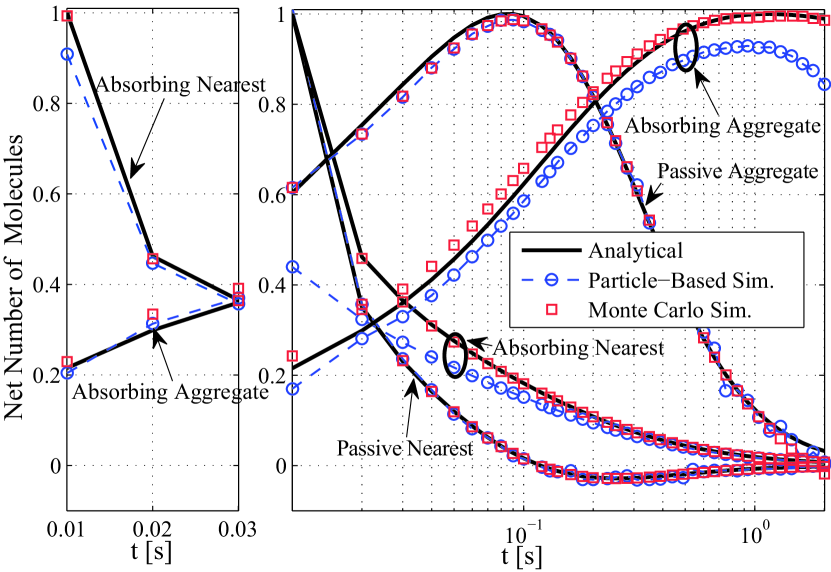
Figure 2: Net number of observed molecules at the receiver as a function of time. All curves are scaled by the maximum value of the analytical curves in the right subplot.

VI Numerical and Simulation Results

Throughout this section, we focus on Monte Carlo approaches to conduct the simulations, which we also compare with particle-based simulations. We consider two types of Monte Carlo simulations. Both types use a HPPP to generate the locations of the transmitters. In the first type, which we use in Figs. 2–5, observations in each realization are “simulated” by adding the expected observation from every transmitter at the sampling time in (11) and (20). In the second type, which we use in Figs. 6–9, observations in each realization are “simulated” by drawing from the Poisson distribution as in (32) and (34), whose mean is the sum of the observations expected from every transmitter at the sampling time. The second type generates distributions of individual observations in order to measure the bit error probability.

In this section, we first validate the Monte Carlo approaches by comparing with particle-based simulations and our analytical results for the net number of molecules at the receiver. Due to the extensive computational demands to simulate large molecular communication environments with a particle-based approach, we then rely on Monte Carlo simulations for further verification of the channel impulse responses and the bit error performance. In all figures of this section, we set $r_{r}=5\,\mu\textnormal{m}$.

TABLE II: The simulation parameters and scaling values applied in Fig. 2.

Transmitter	Receiver	Realizations	Time	Scaling
			Step [s]	Value
Nearest	Passive	$10^{4}$	$10^{-2}$	149.57
Nearest	Absorbing	$10^{4}$	$10^{-2}$	354.52
Aggregate	Passive	$10^{4}$	$10^{-2}$	9.252
Aggregate	Absorbing	$10^{3}$	$10^{-3}$	59.42

In Figs. 2, 3, and 4, we set $N_{\rm{tx}}=10^{4}$, and $k_{d}=0$ to focus on normal diffusion without molecule degradation in a large-scale system. The analytical curves of the expected number of molecules absorbed at the absorbing receiver due to all transmitters, the nearest transmitter, and the other transmitters are plotted using (28), (23), and (24), and are abbreviated as “Absorbing All”, “Absorbing Nearest”, and “Absorbing Aggregate”, respectively. The analytical curves of the expected number of molecules observed inside the passive receiver due to all transmitters, the nearest transmitter, the other transmitters are plotted using (27), (23), and (24), and are abbreviated as “Passive All”, “Passive Nearest”, and “Passive Aggregate”, respectively. The analytical curves and the simulations are occasionally abbreviated as “Anal.” and “Sim.”, respectively.

VI-A Validation of Simulation Approaches

The Monte Carlo approaches assume that the channel response for a single transmitter is correct. We check this assumption by comparing the first Monte Carlo approach with particle-based simulations generated using the simulation algorithm in [11] and the AcCoRD simulator (Actor-based Communication via Reaction-Diffusion) [35]. In the first Monte Carlo approach, every realization is simulated by calculating the net number of molecules due to each transmitter using (11) and (20) for the absorbing and passive receivers, respectively. In the particle-based approach, observations in each realization are “simulated” by placing individual molecules at each transmitter, moving each molecule by Brownian motion, and checking whether each molecule diffused into the passive receiver or was absorbed by the absorbing receiver. AcCoRD simulations are defined by configuration files; here, each configuration file listed the transmitter locations as specified by the current permutation of the HPPP, and each transmitter permutation was simulated at least 10 times.

The simulation approaches are compared in Fig. 2, where we set $D=80\times 10^{-12}\frac{\textnormal{m}^{2}}{\textnormal{s}}$ and assume that the transmitters are placed up to $R_{a}=50\mu$m from the center of the receiver at a density of $\lambda_{a}=10^{-4}$ transmitters per $\mu$m³ (i.e., 52 transmitters on average, including the exclusion of the receiver volume). The receiver takes samples every $T_{ss}=0.01$ s and calculates the net change in the number of observed molecules between samples. The default simulation time step is also $0.01$ s. Unless otherwise noted, all simulation results were averaged over $10^{4}$ transmitter location permutations, as shown in Table II.

In Fig. 2, we verify the analytical expressions for the expected net number of molecules observed during $[t,t+T_{ss}]$ at both receivers in (23), and (24) by comparing with the particle-based simulations and the Monte Carlo simulations. In the right subplot of Fig. 2, we compare passive and absorbing receivers and observe the expected net number of observed molecules during $[t,t+T_{ss}]$ due to the nearest transmitter and due to the other transmitters. In the left subplot of Fig. 2, we lower the simulation time step to $10^{-4}\,\textnormal{s}$ for the first few samples of the two absorbing receiver cases, in order to demonstrate the corresponding improvement in accuracy. All curves in both subplots are scaled by the maximum value of the corresponding analytical curve in the right subplot; the scaling values and other simulation parameters are summarized in Table II.

VI-A1 Particle-Based Simulation Validation

Overall, there is good agreement between the analytical curves and the particle-based simulations in the right subplot of Fig. 2. The analytical results for the net number of molecules observed inside the passive receiver during $[t,t+T_{ss}]$ due to the nearest transmitter are highly accurate, and even captures the net loss of molecules observed after $t=0.1\,\textnormal{s}$. The particle-based simulation of the “Passive Aggregate” case also becomes noisier with increasing $t$ as the normalized net number of molecules goes below 0.3, which is due to the very low number of molecules observed (the scaling factor in this case is only 9.525; see Table II) and can be improved by averaging over more realizations. Both simulation approaches slightly underestimate the analytical curve in the “Passive Aggregate” case for $t<0.1$ s, due to the constraint on the placement of transmitters to within a radius of $R_{a}$ = 50 $\mu$m (which we relax in later figures once we do not include particle-based simulations).

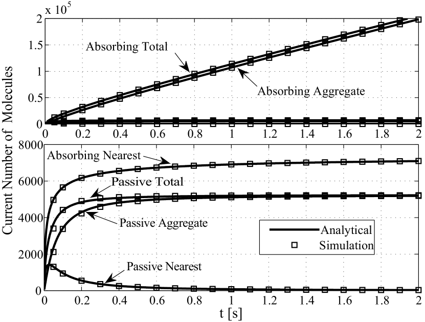
Figure 3: Expected number of molecules observed at the receiver as a function of time.

There is less agreement between the particle-based simulations and the analytical expressions for the absorbing receiver, and this is primarily due to the large simulation time step (even though we used a smaller time step for the aggregate transmitter case in the right subplot; see Table II). To demonstrate the impact of the time step, the left subplot shows much better agreement for the absorbing receiver model by lowering the time step to $10^{-4}\,\textnormal{s}$. This improvement is especially true in the case of the nearest transmitter, as there is significant deviation between the particle-based simulation and the analytical expression for very early times in the right subplot.

VI-A2 Monte Carlo Simulation Validation

There is a good match between the analytical curves and the Monte Carlo simulations for the net number of molecules observed at both types of receivers during $[t,t+T_{ss}]$ due to the nearest transmitter, which can be attributed to the large number of molecules (as shown in Table II) and the small value of the shortest distance between the transmitter and the receiver compared with $R_{a}=50\,\mu\textnormal{m}$. There is slight deviation in the Monte Carlo simulations for the expected number of molecules observed at both types of receivers due to the other transmitters, and this is primarily due to the restricted placement of transmitters to the maximum distance $R_{a}=50\,\mu\textnormal{m}$. In Figs. 3 and 4, better agreement between the analytical curves and Monte Carlo simulation is achieved by increasing the maximum placement distance $R_{a}$.

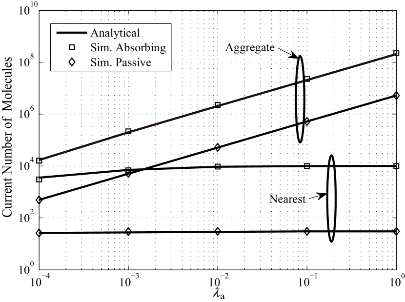
Figure 4: Expected number of molecules observed at the receiver at time $t=2\;\;\textnormal{s}$ as a function of the density of transmitters.

Due to the extensive computational demands to simulate such large molecular communication environments, we assume that the particle-based simulations have sufficiently verified the analytical models. The remaining simulation results in the rest of the figures are only generated via Monte Carlo simulation.

VI-B Channel Impulse Response Evaluation

From Fig. 2 and the scaling values in Table II, we see that the expected net number of molecules observed at the absorbing receiver is much larger than that inside the passive receiver, since every molecule arriving at the absorbing receiver is permanently absorbed. We also notice that the expected net number of observed molecules due to the nearest transmitter is much larger than that due to the other transmitters, which may be due to a relatively low transmitter density.

Figs. 3 and 4 plot the expected number of molecules currently observed at the absorbing receiver and the passive receiver at time $t$ rather than their net change during each sampling interval. In Figs. 3 and 4, we set the parameters: $D=120\times 10^{-12}\frac{\textnormal{m}^{2}}{\textnormal{s}}$, $R_{a}=100\,\mu\textnormal{m}$, and $T_{ss}=0.1\;\textnormal{s}$. We set the density of transmitters as $\lambda_{a}=10^{-3}/\mu\textnormal{m}^{3}$. As shown in the lower subplot of Fig. 3, even though the point transmitters have random locations, the channel responses of the receivers due to the nearest transmitter in this large-scale molecular communication system are consistent with those observed at the absorbing receiver in [11, Fig. 4] and the passive receiver in [6, Fig. 2] and [25, Fig. 1] for a point-to-point molecular communication system.

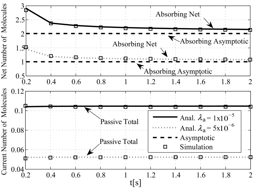
Figure 5: Expected net number of molecules observed at the receiver as a function of time.

In Fig. 3, we notice that the expected number of molecules currently observed at time $t$ due to all transmitters is dominated by the other transmitters, rather than the nearest transmitter, which is due to the increased number of molecules received from the other transmitters with the higher density of transmitters compared to that in Fig. 2. Furthermore, as we might expect, the expected number of molecules currently observed inside the passive receiver at time $t$ stabilizes after $t=0.8\,\textnormal{s}$, whereas that at the absorbing receiver eventually increases linearly with increasing time. This reveals the potential differences in appropriate demodulation design for these two types of receiver. More specifically, unlike the demodulation for passive receiver, demodulation using the number of molecules currently absorbed by the absorbing receiver is not a suitable design, since it cannot have a single optimal threshold.

Fig. 4 plots the expected number of molecules observed at the absorbing receiver and the passive receiver at $t=2\,$s versus the density of transmitters $\lambda_{a}$. With the increase of $\lambda_{a}$, the number of observed molecules due to the other transmitters increases, whereas the number of observed molecules due to the nearest transmitter remains almost unchanged. More importantly, the dominant effect of the other transmitters on the number of observed molecules becomes more obvious as $\lambda_{a}$ increases.

VI-C Demodulation Criteria and Single Bit Error Performance

From Figs. 3 and 4, the current number of absorbed molecules increases with increasing time and transmitter density, thus demodulation based on the current number of molecules absorbed by the absorbing receiver will require an increasing demodulation threshold for larger $t$ and $\lambda_{a}$. Hence, in our model, the demodulation of the absorbing receiver is based on the net number of absorbed molecules, whereas the demodulation of the passive receiver is based on the current number of molecules observed at the receiver. In Figs. 5 and 6, we set $N_{\rm{tx}}=20$, $k_{d}=0$, $T_{b}=0.2$ s, $R_{a}=100\,\mu\textnormal{m}$, $D=80\times 10^{-11}\frac{\textnormal{m}^{2}}{\textnormal{s}}$, and with only a single bit-1 transmitted at $t=0$, i.e., the transmit bit sequence is [1 0 0 0 $\ldots$ ].

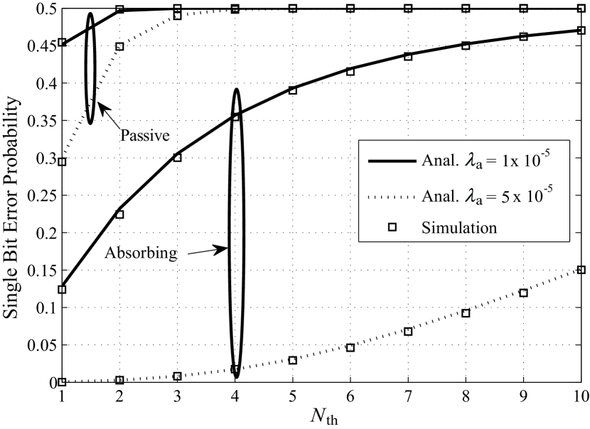
Figure 6: Single bit error probability as a function of threshold.

Fig. 5 plots the net number of molecules absorbed by the absorbing receiver during one bit interval $T_{b}$ in the upper subfigure, and the number of observed molecules at the passive receiver at the end of each bit interval $T_{b}$ in the lower subfigure, each with different transmitter densities. We also plot the asymptotic net number of absorbed molecules using (30) with a dashed line. We see that the net number of molecules absorbed by the absorbing receiver during each bit interval decreases as time increases, and converges to the asymptotic value. The number of observed molecules inside the passive receiver at the end of every bit interval remains comparable as time increases, which suggests that taking multiple samples of the number of observed molecules at different times in one bit interval may not greatly improve the detection reliability. For both receivers, the ISI is not small compared with the observation in the first bit interval, which demonstrates the high ISI in the large-scale molecular communication system.

In Fig. 6, we start using the second Monte Carlo approach for simulations in order to generate distributions of observations, and we plot the single bit error probability of both receivers using (38), in order to focus on the impact of multiple transmitters with no ISI impairment. We notice that the single bit error probability at both receivers improves with increasing $\lambda_{a}$, which is due to the increased number of molecules absorbed by the absorbing receiver during $t\in[0,T_{b}]$, and the increased number of observed molecules inside the passive receiver at $t=T_{b}$ as seen in Fig. 5. Another interesting observation is that the single bit error probability of the passive receiver is much worse than that of the absorbing receiver, which is due to the lower number of observed molecules at the passive receiver than that at the absorbing receiver. Clearly, the two receivers need different demodulation thresholds.

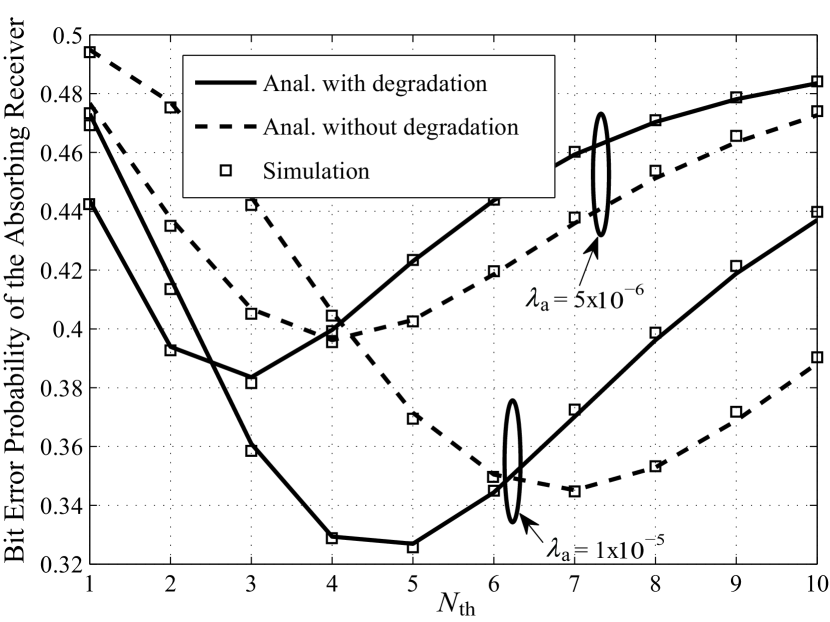
Figure 7: Bit error probability of the absorbing receiver as a function of threshold.

VI-D Multiple Bits Error Performance

Figs. 7 and 8 plot the bit error probabilities of the absorbing receiver and that of the passive receiver in the proposed large-scale molecular communication system, respectively, both with $(k_{d}=0.8$ ${\textnormal{s}}^{-1})$ or without $(k_{d}=0$ ${\textnormal{s}}^{-1})$ molecule degradation. Fig. 9 compares the bit error probabilities of the absorbing receiver and the passive receiver in the proposed large-scale molecular communication system under molecule degradation $(k_{d}=0.8$ ${\textnormal{s}}^{-1})$ using DFD, with that using the simple detector. In Figs. 7, 8, and 9, we set the parameters: $T_{b}=0.2$ s, $R_{a}=100\,\mu\textnormal{m}$, and $D=80\times 10^{-11}\frac{\textnormal{m}^{2}}{\textnormal{s}}$ with a 5 bit sequence transmitted by all transmitters, where the first four bits are set as [1 0 1 0] . We set $N_{\rm{tx}}=20$ in Fig. 7, $N_{\rm{tx}}=300$ in Fig. 8, and $N_{\rm{tx}}=10^{4}$ in Fig. 9.

In Figs. 7 and 8, we see a good match between the analytical results in (38) and the simulations, which demonstrates the correctness of our derivations. We observe that the minimum bit error probability improves with increasing the density of the transmitters. We also see that the minimum bit error probability can be improved by introducing molecule degradation. This can be explained by the fact that many molecules, especially those released far from the receiver, degrade before they reach the receiver, and this reduces the ISI effect. However, the bit error probability with molecule degradation is not always better than without degradation for a given decision threshold, which can be attributed to the fact that the degradation not only reduces the ISI, but also lowers the strength of the intended signal.

In both figures, we notice that the minimum bit error probability is still not low enough for reliable transmission, even though it can be potentially improved by increasing $N_{\rm{tx}}$. This is because with multiple transmitted bits, the ISI will accumulate and keep growing with every transmit bit-1. These observations reveal that the demodulation threshold at each bit should increase with the number of transmit bits, instead of being fixed.

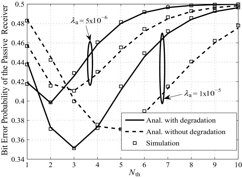
Figure 8: Bit error probability of the passive receiver as a function of threshold.

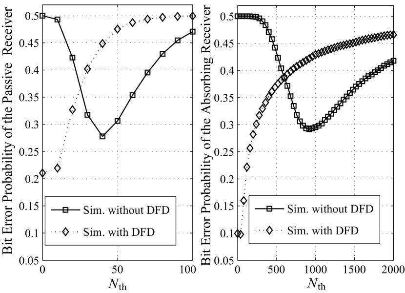
Figure 9: Bit error probability of receivers as a function of threshold.

We now consider the DFD at both receivers to show its potential benefits in improving the bit error probability. Fig. 9 compares the bit error probability of both receivers having molecule degradation during diffusion and DFD during detection with that without DFD during detection using Monte Carlo simulation, where the passive receiver is capable of subtracting the current observation in one previous bit interval $N\left[j-1\right]$ from that in the current bit interval $N\left[j\right]$, and the absorbing receiver is capable of subtracting the net observation in one previous bit interval $N\left[j-1\right]$ from that in the current bit interval $N\left[j\right]$ for the demodulation of the $j$th bit. With DFD, the $j$th bit is decoded based on if $N\left[j\right]-N\left[j-1\right]>N_{\rm{th}}$ or not. By doing so, the accumulated ISI due to the previous bits is mitigated artificially during the demodulation process. We set $\lambda_{a}=5\times 10^{-6}/\mu\textnormal{m}^{3}$. With the help of DFD, we see that the minimum bit error probability of both receivers can be improved for the proposed system.

VII Conclusions and Future Work

In this paper, we provided a general model for the collective signal modelling in a large-scale molecular communication system with or without degradation using stochastic geometry. The collective signal strength at a fully absorbing receiver and a passive receiver is modelled and explicitly characterized. We derived tractable expressions for the expected number of observed molecules at the fully absorbing receiver and the passive receiver, which were shown to increase with transmitter density. We also derived analytical expressions for the bit error probabilities at both receivers with a simple detector taking one sample per bit, and the minimum bit error probabilities were shown to improve with the help of degradation. The analytical model presented in this paper can also be applied for the performance evaluation of other types of receiver (e.g., partially absorbing, reversible adsorption receiver, ligand-binding receiver) in a large-scale molecular communication system by substituting its corresponding channel response.

Appendix A Proof of Proposition 1

According to [36], the probability of finding $k$ nodes in a bounded Borel $A\subset{{\mathbb{R}}^{m}}$ in a homogeneous $m$-dimensional Poisson point process of intensity $\lambda$ is given by

$$\Pr\left({M=k}\right)={e^{-\lambda_{a}\mu\left(A\right)}}\frac{{{{\left({\lambda_{a}\mu\left(A\right)}\right)}^{k}}}}{{k!}},$$ (A.1)

where $M$ is the Poisson random variable, and $\mu\left(A\right)$ is the standard Lebesgue measure of $A$.

Thus, the probability of finding zero nodes in a bounded Borel $A\subset{{\mathbb{R}}^{3}}$ in a homogeneous $3$D Poisson point process of intensity $\lambda_{a}$ is obtained as

$$\Pr\left({M=0}\right)={e^{-\lambda_{a}\mu\left(A\right)}},$$ (A.2)

where $\mu\left(A\right)={\frac{4}{3}\pi{x^{3}}-\frac{4}{3}\pi{r_{r}}^{3}}$, and $x$ is the radius of the bounded ball.

Using ${f_{\left\|{{x^{*}}}\right\|}}(x)=-\frac{{d\Pr\left({N=0}\right)}}{{dx}}$, we prove (21).

Appendix B Proof of Theorem 1

Based on (10) and (20), we can write the expected net number of molecules observed at the receiver as

$${\mathbb{E}} \left\{N_{{\rm{all}}}\left({{{\Omega_{{r_{r}}}},t,t+{T_{ss}}}}\right)\right\}={\mathbb{E}}\Big{\{}\sum\limits_{x\in\Phi_{a}}{{N_{\rm{tx}}}\Phi\left(r\right)}\Big{\}},$$ (B.1)

where

$$\Phi\left(r\right)={F^{{\rm{FA}}}}\left({\left.{{\Omega_{{r_{r}}}},t,t+{T_{ss}}}\right|r}\right),$$ (B.2)

for the absorbing receiver, and

$$\Phi\left(r\right)={F^{{\rm{PS}}}}\left({\left.{{\Omega_{{r_{r}}}},t+{T_{ss}}}\right|r}\right)-{F^{{\rm{PS}}}}\left({\left.{{\Omega_{{r_{r}}}},t}\right|r}\right),$$ (B.3)

for the passive receiver.

According to the Campbell’s theorem in 3D space, the mean of the random sum of a point process $\Phi_{a}$ on ${\mathbb{R}}^{3}$ and ${{N_{\rm{tx}}}\Phi\left(r\right)}$ is given as [27, Eq. (1.18)]

$${\mathbb{E}}\left\{N_{{\rm{all}}}\left({{{\Omega_{{r_{r}}}},t,t+{T_{b}}}}\right)\right\} =\int_{{{\mathbb{R}}^{3}}}{\left[{N_{{\rm{tx}}}\Phi\left(r\right)}\right]{\lambda_{a}}\mathop{}\!\mathrm{d}x}$$

$$={\lambda_{a}}\int_{{r_{r}}}^{\infty}{\left[{N_{{\rm{tx}}}\Phi\left(r\right)}\right]3\frac{{4\pi}}{3}{r^{2}}\mathop{}\!\mathrm{d}r}.$$ (B.4)

Thus, we derive

$${\mathbb{E}} \left\{N_{{\rm{all}}}\left({{{\Omega_{{r_{r}}}},t,t+{T_{ss}}}}\right)\right\}=4\pi{\lambda_{a}}{N_{\rm{tx}}^{\rm{FA}}}\int_{{r_{r}}}^{\infty}{\Phi\left(r\right)}{r^{2}}\mathop{}\!\mathrm{d}r.$$ (B.5)

Appendix C Proof of Lemma 1

With $k_{d}=0$, we rewrite (B.5) using $z=r-r_{r}$ as

$${\mathbb{E}}\left\{N_{{\rm{all}}}^{{\rm{FA}}}\left({{{\Omega_{{r_{r}}}},t,t+{T_{ss}}}}\right)\right\}=$$

$$\hskip 4.26773pt\frac{{\sqrt{4\pi}{\lambda_{a}}{{N_{\rm{tx}}}}{r_{r}}}}{{\sqrt{D}}}\int_{t}^{t+{T_{ss}}}{\int_{0}^{\infty}{z\left({z+{r_{r}}}\right)\exp\big{(}{-\frac{{{z^{2}}}}{{4Dx}}}\big{)}\mathop{}\!\mathrm{d}z}}\frac{1}{{\sqrt{{x^{3}}}}}\mathop{}\!\mathrm{d}x$$

$$\hskip 4.26773pt=\frac{{\sqrt{4\pi}{\lambda_{a}}{N_{\rm{tx}}}{r_{r}}}}{{\sqrt{D}}}\Bigg{[}{\int_{t}^{t+{T_{ss}}}{\int_{0}^{\infty}{{z^{2}}\exp\big{(}{-\frac{{{z^{2}}}}{{4Dx}}}\big{)}\mathop{}\!\mathrm{d}z}}\frac{1}{{\sqrt{{x^{3}}}}}\mathop{}\!\mathrm{d}x}\Bigg{.}$$

$$\hskip 5.69046pt\Bigg{.}{+{r_{r}}\int_{t}^{t+{T_{ss}}}{\int_{0}^{\infty}{z\exp\big{(}{-\frac{{{z^{2}}}}{{4Dx}}}\big{)}\mathop{}\!\mathrm{d}z}}\frac{1}{{\sqrt{{x^{3}}}}}\mathop{}\!\mathrm{d}x}\Bigg{]},$$ (C.1)

With mathematical manipulations, we simplify (C.1) as

$${\mathbb{E}}\left\{N_{{\rm{all}}}^{{\rm{FA}}}\left({{{\Omega_{{r_{r}}}},t,t+{T_{ss}}}}\right)\right\}$$

$$\hskip 4.26773pt=4\sqrt{\pi}{\lambda_{a}}{N_{\rm{tx}}}{r_{r}}\Bigg{[}{D\sqrt{\pi}\int_{t}^{t+{T_{ss}}}{\mathop{}\!\mathrm{d}x}+\sqrt{D}{r_{r}}\int_{t}^{t+{T_{ss}}}{\frac{1}{{\sqrt{x}}}\mathop{}\!\mathrm{d}x}}\Bigg{]}.$$ (C.2)

Solving (C.2), we prove Lemma 1.

Appendix D Proof of Theorem 2

Based on the fact that

$${\left.{\frac{{{\partial^{n}}\left({\exp\left\{{-N_{{\rm{tx}}}\phi x\tau}\right\}}\right)}}{{\partial{x^{n}}}}}\right|_{x={\phi^{-1}}}}=\exp\left\{{-N_{{\rm{tx}}}\tau}\right\}{\left({-N_{{\rm{tx}}}\phi\tau}\right)^{n}},$$ (D.1)

we rewrite the error probability for the transmit bit-1 signal in the $j$th bit as

$${P_{e}}\left[{\hat{b}_{j}=0\left|{b_{j}=1}\right.}\right]=\int_{0}^{\infty}{\exp\left\{{-{N_{{\rm{tx}}}}\tau}\right\}}{f_{R_{\rm{tot}}^{j}}}\left(\tau\right)\mathop{}\!\mathrm{d}\tau+$$

$$\sum\limits_{n=1}^{{N_{{\rm{th}}}}-1}{\frac{1}{{{{\left({-\phi}\right)}^{n}}n!}}\int_{0}^{\infty}{{{\left.{\frac{{{\partial^{n}}\left({\exp\left\{{-{N_{{\rm{tx}}}}\phi x\tau}\right\}}\right)}}{{\partial{x^{n}}}}}\right|}_{x={\phi^{-1}}}}}{{f_{R_{\rm{tot}}^{j}}}\left(\tau\right)\mathop{}\!\mathrm{d}\tau}}$$

$$={\mathscr{L}_{R_{\rm{tot}}^{j}}}\left({{N_{{\rm{tx}}}}}\right)+{\sum\limits_{n=1}^{{N_{{\rm{th}}}}-1}{\frac{1}{{{{\left({-\phi}\right)}^{n}}n!}}\left.{\frac{{{\partial^{n}}\left[{{\mathscr{L}_{R_{\rm{tot}}^{j}}}\left({{N_{{\rm{tx}}}}\phi x}\right)}\right]}}{{\partial{x^{n}}}}}\right|}_{{}_{x={\phi^{-1}}}}},$$ (D.2)

where ${{f_{R_{\rm{tot}}^{j}}}\left(\tau\right)}$ is the PDF of ${R_{\rm{tot}}^{j}}$, and ${\mathscr{L}_{R_{\rm{tot}}^{j}}}\left(\cdot\right)$ is the Laplace transform of ${R_{\rm{tot}}^{j}}$.

According to (E.4), the Laplace transform of ${R_{\rm{tot}}^{j}}$ can be represented as

$${\mathscr{L}_{R_{\rm{tot}}^{j}}}\left(s\right)= {\mathbb{E}}\Big{[}{\exp\Big{\{}{-s{\sum_{{\Phi_{a}}}}R\left({\left.{{\Omega_{{r_{r}}}},j}\right|\left\|{\bf{x}}\right\|}\right)}\Big{\}}}\Big{]}$$

$$= {\mathbb{E}}\Big{[}{\prod\limits_{{\Phi_{a}}}{\exp\left\{{-sR\left({\left.{{\Omega_{{r_{r}}}},j}\right|\left\|{\bf{x}}\right\|}\right)}\right\}}}\Big{]}$$

$$=\exp\left\{{-{\lambda_{a}}\int_{{{\mathbb{R}}^{3}}}{\left({1-\exp\left\{{-sR\left({\left.{{\Omega_{{r_{r}}}},j}\right|\left\|{\bf{x}}\right\|}\right)}\right\}}\right)\mathop{}\!\mathrm{d}\left\|{\bf{x}}\right\|}}\right\}$$

$$=\exp\left\{{-{\lambda_{a}}\int_{{r_{r}}}^{\infty}{\left({1-\exp\left\{{-sR\left({\left.{{\Omega_{{r_{r}}}},j}\right|r}\right)}\right\}}\right)}4\pi{r^{2}}\mathop{}\!\mathrm{d}r}\right\}.$$ (D.3)

Based on (D.3) and the Fa$\grave{\text{a}}$ di Bruno’s formula [37], we derive

$${\left.{\frac{{{\partial^{n}}\left[{{\mathscr{L}_{R_{\rm{tot}}^{j}}}\left({{N_{{\rm{tx}}}}\phi x}\right)}\right]}}{{\partial{x^{n}}}}}\right|}_{{}_{x={\phi^{-1}}}}=$$

$$\hskip 5.69046pt\exp\left\{{-{\lambda_{a}}\int_{{r_{r}}}^{\infty}{\left({1-\exp\left\{{-{N_{{\rm{tx}}}}R\left({\left.{{\Omega_{{r_{r}}}},j}\right|r}\right)}\right\}}\right)}4\pi{r^{2}}\mathop{}\!\mathrm{d}r}\right\}$$

$$\hskip 5.69046pt\times{\sum^{n}}{\frac{{n!}}{{\prod\limits_{k=1}^{n}{{n_{k}}!k{!^{{n_{k}}}}}}}}\prod\limits_{k=1}^{n}{\Big{[}{-{\lambda_{a}}\int_{{r_{r}}}^{\infty}{\big{[}{-{{\left({-{N_{{\rm{tx}}}}\phi R\left({\left.{{\Omega_{{r_{r}}}},j}\right|r}\right)}\right)}^{k}}}\big{.}}}\Big{.}}$$

$$\hskip 5.69046pt\times{\Big{.}{\big{.}{\exp\left\{{-{N_{{\rm{tx}}}}R\left({\left.{{\Omega_{{r_{r}}}},j}\right|r}\right)}\right\}}\Big{]}4\pi{r^{2}}\mathop{}\!\mathrm{d}r}\Big{]}^{{n_{k}}}},$$ (D.4)

where the summation $\sum\limits^{n}$ is over all n-tuples of nonegative integers ($n_{1},...,n_{n}$) satisfying the constraint $1\cdot{n_{1}}+2\cdot{n_{2}}+\cdots+k\cdot{n_{k}}+\cdots+n\cdot{n_{n}}=n$. Noting that $\prod\limits_{k=1}^{n}{{{\left({-\phi}\right)}^{k{n_{k}}}}=}{\left({-\phi}\right)^{n}}$, and substituting (D.3) and (D.4) into (D.2), we finally derive (39). We can follow a similar method to derive (40).

Appendix E Proof of Lemma 3

With fixed threshold-based demodulation, the error probability with the transmit bit-1 signal in the $j$th bit is represented as

$${P_{e}}\left[{{{\hat{b}}_{j}}=0\left|{{b_{j}}=1,{b_{1:j-1}}}\right.}\right]=\Pr\left[{N\left[j\right]<1}\right]$$

$$\approx{{\mathbb{E}}_{R_{\rm{tot}}^{j}}}\left\{{\Pr\left[{\left.{{P}\left({{N_{{\rm{tx}}}}R_{\rm{tot}}^{j}}\right)<1}\right|R_{\rm{tot}}^{j}}\right]}\right\}$$

$$={{\mathbb{E}}_{R_{\rm{tot}}^{j}}}\left\{{\sum\limits_{n=0}^{0}{\frac{1}{{n!}}\exp\left\{{-{N_{{\rm{tx}}}}R_{\rm{tot}}^{j}}\right\}{{\left({{N_{{\rm{tx}}}}R_{\rm{tot}}^{j}}\right)}^{n}}}}\right\}$$

$$={\mathscr{L}_{R_{\rm{tot}}^{j}}}\left({N_{{\rm{tx}}}}\right),$$ (E.1)

where

$$R_{\rm{tot}}^{j}=\sum\limits_{x\in{\Phi_{a}}}{R\left({\left.{{\Omega_{{r_{r}}}},j}\right|\left\|{\bf{x}}\right\|}\right)},$$ (E.2)

with ${R\left({\left.{{\Omega_{{r_{r}}}},j}\right|\left\|{\bf{x}}\right\|}\right)}$ given in (36) for the absorbing receiver and in (37) for the passive receiver. Substituting (D.3) into (E.1), we derive (41). We can follow a similar method to derive (42).

With the threshold-based demodulation, the error probability for a transmit bit-1 signal in the $j$th bit is represented as

$${P_{e}}\left[{\hat{b}_{j}=0\left|{b_{j}=1}\right.}\right]=\Pr\left[{N\left[j\right]<{N_{{\rm{th}}}}}\right]$$

$$\approx{{\mathbb{E}}_{R_{{\rm{tot}}}^{j}}}\left\{{\Pr\left[{\left.{{P}\left({{N_{{\rm{tx}}}}R_{{\rm{tot}}}^{j}}\right)<{N_{{\rm{th}}}}}\right|R_{\rm{tot}}^{j}}\right]}\right\}$$

$$={{\mathbb{E}}_{R_{\rm{tot}}^{j}}}\left\{{\sum\limits_{n=0}^{{N_{{\rm{th}}}}-1}{\frac{1}{{n!}}\exp\left\{{-{N_{{\rm{tx}}}}R_{\rm{tot}}^{j}}\right\}{{\left({{N_{{\rm{tx}}}}R_{\rm{tot}}^{j}}\right)}^{n}}}}\right\}$$

$$=\sum\limits_{n=0}^{{N_{{\rm{th}}}}-1}{\frac{1}{{n!}}\int_{0}^{\infty}{\exp\left\{{-N_{{\rm{tx}}}\tau}\right\}{{\left({N_{{\rm{tx}}}\tau}\right)}^{n}}}\mathop{}\!\mathrm{d}\Pr\left({R_{\rm{tot}}^{j}\leq\tau}\right)},$$ (E.3)

where

$$R_{\rm{tot}}^{j}=\sum\limits_{x\in{\Phi_{a}}}{R\left({\left.{{\Omega_{{r_{r}}}},j}\right|\left\|{\bf{x}}\right\|}\right)},$$ (E.4)

with ${R\left({\left.{{\Omega_{{r_{r}}}},j}\right|\left\|{\bf{x}}\right\|}\right)}$ given in (36) for the absorbing receiver and in (37) for the passive receiver.

References

- [1] Y. Deng, A. Noel, W. Guo, A. Nallanathan, and M. Elkashlan, “Stochastic geometry model for large-scale molecular communication systems,” in Proc. IEEE GLOBECOM, Dec. 2016.
- [2] T. Nakano, A. Eckford, and T. Haraguchi, Molecular communication. Cambridge University Press, 2013.
- [3] E. Codling, M. Plank, and S. Benhamous, “Random walk models in biology,” Journal of The Royal Society Interface, vol. 5, no. 25, pp. 813–834, Aug. 2008.
- [4] S. Atkingson and P. Williams, “Quorum sensing and social networking in the microbial world,” Journal of The Royal Society Interface, vol. 6, no. 40, pp. 959–978, Aug. 2009.
- [5] W. Guo, Y. Deng, H. B. Yilmaz, N. Farsad, M. Elkashlan, C. Chae, A. W. Eckford, and A. Nallanathan, “SMIET: simultaneous molecular information and energy transfer,” IEEE Wireless Comm., 2017.
- [6] I. Llatser, A. Cabellos-Aparicio, and M. Pierobon, “Detection techniques for diffusion-based molecular communication,” IEEE J. Sel. Areas Commun., vol. 31, pp. 726–734, Dec. 2013.
- [7] W. Guo, C. Mias, N. Farsad, and J. Wu, “Molecular versus electromagnetic wave propagation loss in macro-scale environments,” IEEE Trans. Mol. Biol. Multi-Scale Commun., vol. 1, Mar. 2015.
- [8] H. C. Berg, Random Walks in Biology. Princeton University Press, 1993.
- [9] M. S. Kuran, H. B. Yilmaz, T. Tugcu, and B. O. Edis, “Energy model for communication via diffusion in nanonetworks,” Nano Commun. Netw., vol. 1, no. 2, pp. 86–95, Apr. 2010.
- [10] H. B. Yilmaz and C.-B. Chae, “Simulation study of molecular communication systems with an absorbing receiver: Modulation and ISI mitigation techniques,” Simulat. Modell. Pract. Theory, vol. 49, pp. 136–150, Dec. 2014.
- [11] Y. Deng, A. Noel, M. Elkashlan, A. Nallanathan, and K. C. Cheung, “Modeling and simulation of molecular communication systems with a reversible adsorption receiver,” IEEE Trans. Mol. Biol. Multi-Scale Commun., vol. 1, no. 4, pp. 347–362, Dec. 2015.
- [12] B. Tepekule, A. E. Pusane, H. B. Yilmaz, C. B. Chae, and T. Tugcu, “ISI mitigation techniques in molecular communication,” IEEE Trans. Mol. Biol. Multi-Scale Commun., vol. 1, no. 2, pp. 202–216, Jun. 2015.
- [13] P. J. Shih, C. H. Lee, P. C. Yeh, and K. C. Chen, “Channel codes for reliability enhancement in molecular communication,” IEEE J. Sel. Areas Commun., vol. 31, no. 12, pp. 857–867, Dec. 2013.
- [14] S. M. Douglas, I. Bachelet, and G. M. Church, “A logic-gated nanorobot for targeted transport of molecular payloads,” Science, vol. 335, no. 6070, pp. 831–834, Feb. 2012.
- [15] A. Cavalcanti, T. Hogg, B. Shirinzadeh, and H. Liaw, “Nanorobot communication techniques: A comprehensive tutorial,” in Proc. IEEE Int. Conf. Control, Autom., Robot., Vis., Dec. 2006, pp. 1–6.
- [16] A. Noel, K. C. Cheung, and R. Schober, “A unifying model for external noise sources and ISI in diffusive molecular communication,” IEEE J. Sel. Areas Commun., vol. 32, no. 12, pp. 2330–2343, Dec. 2014.
- [17] G. Aminian, M. Farahnak-Ghazani, M. Mirmohseni, M. Nasiri-Kenari, and F. Fekri, “On the capacity of point-to-point and multiple-access molecular communications with ligand-receptors,” IEEE Trans. Mol. Biol. Multi-Scale Commun., vol. 1, no. 4, pp. 331–346, Dec. 2015.
- [18] M. Pierobon and I. F. Akyildiz, “A statistical–physical model of interference in diffusion-based molecular nanonetworks,” IEEE Trans. Commun., vol. 62, no. 6, pp. 2085–2095, Jun. 2014.
- [19] M. Haenggi, Stochastic geometry for wireless networks. Cambridge, UK: Cambridge Uni. Press, 2012.
- [20] A. Hasan and J. G. Andrews, “The guard zone in wireless ad hoc networks,” IEEE Trans. Wireless Commun., vol. 6, no. 3, pp. 897–906, Mar. 2007.
- [21] T. D. Novlan, H. S. Dhillon, and J. G. Andrews, “Analytical modeling of uplink cellular networks,” IEEE Trans. Wireless Commun., vol. 12, no. 6, pp. 2669–2679, Jun. 2013.
- [22] Y. Deng, L. Wang, M. Elkashlan, A. Nallanathan, and R. K. Mallik, “Physical layer security in three-tier wireless sensor networks: A stochastic geometry approach,” IEEE Trans. Inf. Forensics Security, to appear 2016.
- [23] Y. Deng, L. Wang, M. Elkashlan, M. Direnzo, and J. Yuan, “Modeling and analysis of wireless power transfer in heterogeneous cellular networks,” IEEE Trans. Commun., no. 99, pp. 1–1, Jul. 2016.
- [24] S. Jeanson, J. Chadoeuf, M. Madec, S. Aly, J. Floury, T. F. Brocklehurst, and S. Lortal, “Spatial distribution of bacterial colonies in a model cheese,” Applied and Environmental Microbiology, vol. 77, no. 4, pp. 1493–1500, Dec. 2010.
- [25] A. Noel, K. C. Cheung, and R. Schober, “Improving receiver performance of diffusive molecular communication with enzymes,” IEEE Trans. Nanobiosci., vol. 13, no. 1, pp. 31–43, Mar. 2014.
- [26] H. B. Yilmaz, A. C. Heren, T. Tugcu, and C.-B. Chae, “Three-dimensional channel characteristics for molecular communications with an absorbing receiver,” IEEE Commun. Lett., vol. 18, no. 6, pp. 929–932, Jun. 2014.
- [27] F. Baccelli and B. Blaszczyszyn, Stochastic geometry and wireless networks: Volume 1: Theory. Now Publishers Inc, 2009, vol. 1.
- [28] K. Schulten and I. Kosztin, Lectures in Theoretical Biophysics, 2000.
- [29] E. L. Cussler, Diffusion: Mass Transfer in Fluid Systems. Cambridge university press, 2009.
- [30] A. C. Heren, H. B. Yilmaz, C. B. Chae, and T. Tugcu, “Effect of degradation in molecular communication: Impairment or enhancement?” IEEE Trans. Mol. Biol. Multi-Scale Commun., vol. 1, no. 2, pp. 217–229, Jun. 2015.
- [31] A. Ahmadzadeh, H. Arjmandi, A. Burkovski, and R. Schober, “Reactive receiver modeling for diffusive molecular communication systems with molecule degradation,” in Proc. IEEE ICC, May 2016, pp. 1–7.
- [32] A. Noel, K. C. Cheung, and R. Schober, “Overcoming noise and multiuser interference in diffusive molecular communication,” in Proc. ACM NANOCOM, May 2014, pp. 1:1–1:9.
- [33] P. Nelson, Biological Physics: Energy, Information, Life, updated 1st ed. W. H. Freeman and Company, 2008.
- [34] A. Noel, K. C. Cheung, and R. Schober, “Using dimensional analysis to assess scalability and accuracy in molecular communication,” in Proc. IEEE ICC MoNaCom, Jun. 2013, pp. 818–823.
- [35] A. Noel, K. C. Cheung, R. Schober, D. Makrakis, and A. Hafid, “Simulating with AcCoRD: Actor-based communication via reaction–diffusion,” Nano Commun. Netw., to appear. [Online]. Available: http://doi.org/10.1016/j.nancom.2017.02.002
- [36] M. Haenggi, “On distances in uniformly random networks,” IEEE Trans. Inf. Theory, vol. 51, pp. 3584–3586, Oct. 2005.
- [37] S. Roman, “The formula of Faa di Bruno,” American Mathematical Monthly, pp. 805–809, 1980.