Second-order Temporal Pooling for Action Recognition

Abstract

Deep learning models for video-based action recognition usually generate features for short clips (consisting of a few frames); such clip-level features are aggregated to video-level representations by computing statistics on these features. Typically zero-th (max) or the first-order (average) statistics are used. In this paper, we explore the benefits of using second-order statistics. Specifically, we propose a novel end-to-end learnable feature aggregation scheme, dubbed temporal correlation pooling that generates an action descriptor for a video sequence by capturing the similarities between the temporal evolution of clip-level CNN features computed across the video. Such a descriptor, while being computationally cheap, also naturally encodes the co-activations of multiple CNN features, thereby providing a richer characterization of actions than their first-order counterparts. We also propose higher-order extensions of this scheme by computing correlations after embedding the CNN features in a reproducing kernel Hilbert space. We provide experiments on benchmark datasets such as HMDB-51 and UCF-101, fine-grained datasets such as MPII Cooking activities and JHMDB, as well as the recent Kinetics-600. Our results demonstrate the advantages of higher-order pooling schemes that when combined with hand-crafted features (as is standard practice) achieves state-of-the-art accuracy.

1 Introduction

The recent resurgence of efficient deep learning architectures has facilitated significant advances in several fundamental problems in computer vision, including human action recognition. For example, recent efforts towards action recognition using LSTM models Karpathy et al. (2014); Donahue et al. (2014), 3D convolutional filters Tran et al. (2015); Carreira and Zisserman (2017), and the two stream models and their extensions Simonyan and Zisserman (2014); Feichtenhofer et al. (2017, 2016b) have pushed the state-of-the-art performances on standard action recognition benchmarks significantly beyond what was possible using hand-crafted features alone Wang et al. (2013b, 2015). However, despite these breakthroughs, the problem of action recognition is far from solved and continues to be challenging in a general setting. Real-world actions are often different from each other in very subtle ways (e.g., washing plates versus washing hands), may have strong appearance variations (e.g., slicing cucumbers versus slicing tomatoes), may involve significant occlusions of objects or human-body parts, may involve background activities, may use hard-to-detect objects (such as knives, peelers, etc.), and may happen over varying durations or at different rates. In this paper, we explore various second-order schemes to address some of these issues. While our schemes are applicable in a general setting, we also explore their suitability in a fine-grained setting that is comprised of activities having low inter-class diversity, and high intra-class diversity Rohrbach et al. (2012).

Most successful recent algorithms for human action recognition Simonyan and Zisserman (2014); Feichtenhofer et al. (2016b); Wang et al. (2016); Srivastava et al. (2015); Yue-Hei Ng et al. (2015); Carreira and Zisserman (2017) are extensions of convolutional neural network (CNN) models originally designed for image-based recognition tasks Krizhevsky et al. (2012). However, in contrast to images, video data is volumetric, and thus extending such image-based models leads to huge computational and memory overheads, which are difficult to be addressed under currently available hardware platforms. A work-around, that is often found to be promising, is to reduce the video-based recognition problem into simpler image-sized subproblems, the results from these sub-problems are later collated in a fusion layer to generate predictions for the full video. While single frames might be insufficient to capture the actions effectively as they lack any temporal aspect, using longer clips demands more CNN parameters, and thus requires more training data and computational resources. As a result, popular deep action classifiers are trained on tiny sub-sequences (of 10–16 frames); the predictions from which are pooled to generate sequence level representations Simonyan and Zisserman (2014); Tran et al. (2015).

Typically, max-pooling or average pooling of the sub-sequence level predictions is used Simonyan and Zisserman (2014); Karpathy et al. (2014); Wang et al. (2015). Although, such pooling operations are easy to implement and fast to compute, they ignore valuable higher-level information contained in the independent predictions that could improve the recognition Cherian et al. (2017a); Koniusz et al. (2016); Peng et al. (2016); Cherian et al. (2017b). For example, in the context of fine-grained recognition, let us consider two activities:  washing plates and  wiping plates. As is clear, discriminating these two actions is not easy due to their appearance similarities. Suppose sequences for the former also incorporate an overlapping activity, say running water from tap (which is absent in the latter). If we compute clip-level features, it is likely that some of the clips in the former will be confused between washing plates and running water from tap; however such a confusion is absent in wiping plates. We propose to make use of such confusions to produce a better action representation. In the above example, we compute the co-occurrences of clip-level action classifier scores for the two activities (viz. washing plates and wiping plates), and then train an action classifier on these co-occurrences. As the underlying classifier confusions are strongly-correlated, the co-occurrence matrix will capture these correlations for better action discrimination, as against using weaker statistics such as average or max pooling.

In this paper, we propose temporal correlation pooling (TCP), a second-order feature pooling scheme, that takes as input a temporal sequence of CNN features (from any intermediate layer), one per video frame (Section 3.4). Each dimension of the features across time can be viewed as a feature trajectory corresponding to the temporal evolution of activations of the respective CNN filters. TCP summarizes these trajectories into a symmetric positive definite (SPD) matrix, each entry of this matrix capturing the similarities between such trajectories. There are several benefits that such a representation offers in contrast to prior approaches, namely (i) SPD matrices, although spanning a Euclidean subspace, are often viewed through the lens of Riemannian geometry, which offers rich non-linear distance measures for similarity computations that may help extract useful cues for recognition, (ii) SPD matrices can be naturally viewed as Mercer kernels, and similarities could be computed after embedding the feature trajectories in an infinite dimensional reproducing kernel Hilbert space (RKHS), thereby enhancing their representational power, and (iii) incorporating prior information is straightforward via sum or product kernels to the SPD kernel.

On the downside, TCP descriptors are quadratic in the size of the input features, which may be infeasible when high-dimensional features from intermediate CNN layers are used. To circumvent this issue, we propose block-diagonal correlation matrix approximations using product quantization and model averaging. Each block matrix in the resulting representation is a small positive definite matrix and thus the above recognition framework can be directly applied.

Another shortcoming of our pooling scheme is related to the strength of the underlying CNN model; if this model is not effective in providing reliable features, the generated descriptor will be ineffective for recognition. Although, we base our CNN on the popular two-stream model (using RGB frames for context and short stack of optical flow images for representing action dynamics), such a model is deficient in two aspects: (i) long-range temporal evolution of actions, and (ii) coupling between appearance and dynamics. While, there are several recent methods that try to address these weaknesses Yue-Hei Ng et al. (2015); Wang et al. (2016); Feichtenhofer et al. (2016b), we propose a simpler workaround that is computationally very cheap, while empirically beneficial. Specifically, we propose a novel video representation dubbed Stacked Mean of Absolute Image Differences (SMAID) that is based on averaging and stacking the absolute differences of a small set of consecutive video frames. Our experiments show that SMAID captures cues complementary to appearances and optical flow, and when combined, demonstrates superior frame-level predictions, especially when the video background is stationary. Incorporating this representation, we propose a three-stream end-to-end learnable CNN framework consisting of a single frame RGB stream for action context, ten-channel optical flow stream for capturing local dynamics, and a SMAID stream capturing long-range dynamics by using subsequences, say up to 45 frames (Section 5).

We provide experiments (Section 8) on four widely-used action recognition datasets to substantiate the effectiveness of our proposed schemes. We also report results using the recent Kinetics-600 dataset Zisserman et al. (2017), that consists of over 400K video clips, thus exploring the scalability of our approach. Our results demonstrate that the SMAID image representation and the correlation pooling schemes demonstrate significant gains on the fine-grained task (about 4–6%) as we expect given our motivation above. Surprisingly, they also showcase competitive performances against recent state-of-the-art methods for general action recognition.

Before moving on, we summarize the main contributions of this paper.

• We propose a novel second-order pooling scheme, dubbed temporal correlation pooling (TCP)

• We propose a kernelized variant of this pooling scheme by embedding the CNN features in an RKHS, dubbed kernelized correlation pooling (KCP)

• We address the scalability of TCP when using higher-dimensional CNN features via our block-diagonal kernelized correlation pooling (BKCP).

• To boost frame-level CNN predictions we propose an enhanced clip-level video representation called SMAID.

• We propose a novel three-stream CNN action recognition model, that learns actions fusing appearance (single RGB frames), short-term (stack of optical flow), and long-term (SMAID) cues.

• We present an end-to-end learnable variant of our CNN by providing expressions for back-propagating the gradients of a classification loss computed using TCP descriptors.

• We provide extensive experimental comparisons on four benchmark datasets and the recently introduced Kinetics-600 dataset, demonstrating state-of-the-art performance.

2 Related Work

There is an enormous breadth of approaches aimed at tackling the problem of activity recognition. We restrict attention in this literature review to methods that have similarities to ours and refer the interested reader to recent surveys Herath et al. (2017); Chaquet et al. (2013) for a detailed study of this topic.
Hand-crafted Features: Typically, in this class of methods, features derived from spatio-temporal interest points, such as dense trajectories, HOG, SIFT, HOF, etc., are extracted from regions of interest and combined to train a discriminative classifier for action recognition. Popular methods, such as those of Wang et al. (2013b) and Laptev (2005), belong to this category. There have been extensions of these methods to use second-order statistical information of features via resorting to Fisher vectors (FV) in Wang and Schmid (2013); Sadanand and Corso (2012); Oneata et al. (2013) and stacks of FVs Peng et al. (2014). While we also employ higher-order statistics, we differ from these techniques in the way we encode this information. Specifically, FVs are the parameter gradients of data modeled using a Gaussian mixture models (GMM). In contrast, our method assumes the underlying CNN implicitly captures the distribution of feature vectors, and uses the empirical covariance matrix of the probabilistic evolution of classifier scores as a representation for data. Our experiments demonstrate that the proposed representation captures complementary cues to FVs, and the synergy that comes from combining our TCP encoding with FVs results in improved accuracy (Section 8).
Deep Learning Methods: It is by now well-known that learning features in a data-driven way using deep learning can lead to better action representation Krizhevsky et al. (2012); Simonyan and Zisserman (2014); Ji et al. (2013); Tran et al. (2015); Donahue et al. (2014); Yue-Hei Ng et al. (2015). However, as alluded to above, scarcity of annotated video data, concomitant to the demand for expensive computational resources, makes adaptability of existing machine learning algorithms to this data modality challenging; thereby demanding efficient video representations. One of the most successful of deep learning methods for action recognition is the two-stream CNN model proposed in (Simonyan and Zisserman, 2014), which decouples the spatial and temporal streams, thereby learning context and action dynamics separately. These streams are trained densely and independently; and at test time, their predictions are pooled. There have been extensions to this basic architecture using deeper networks and fusion of intermediate CNN layers Feichtenhofer et al. (2016b, a); Wang et al. (2016, 2015). We also follow this trend and use a two-stream model as our baseline framework. However, we differ from these techniques in the way we use the CNN features for action recognition (first-order versus second-order). In addition, we also propose a novel three-stream CNN architecture using our SMAID image representation.

We also note that there have been several other deep learning models devised for action modeling such as using 3D convolutional filters Tran et al. (2015); Carreira and Zisserman (2017), recurrent neural networks Baccouche et al. (2011), long-short term memory networks Donahue et al. (2014); Yue-Hei Ng et al. (2015), and large scale video classification architectures Karpathy et al. (2014). These models demand huge collections of videos for effective training, which may be unavailable (e.g., for fine-grained activity tasks). Further, training such models with recurrent structure is also often difficult Pascanu et al. (2013). However, the recent emergence of very large datasets such as Kinetics-400, Kinetics-600 Zisserman et al. (2017), AVA Gu et al. (2017), Moments in Time Monfort et al. (2018), etc. have partially addressed the data issue. Nevertheless, state-of-art models (including 3D convolutional models Carreira and Zisserman (2017)) still use clip-level feature representations that need to be aggregated via suitable pooling schemes for the final video representation or classification; thus the pooling schemes proposed in this paper are complementary to advances in CNN architectures for the action recognition problem.

Pooling Methods: Pooling has been an effective strategy for reducing the complexity of video representations and making them amenable to learning techniques. To this end, temporal pooling schemes have been proposed, such as 3D spatio-temporal gradients Klaser et al. (2008) and STIP features Laptev (2005). More recently, rank pooling has been proposed as an effective way for encoding the temporal evolution of actions (see, for example, Fernando et al. (2015a); Wang et al. (2017); Cherian et al. (2017a, 2018); Wang et al. (2018)). Rank pooling, however, requires solving an order-constrained quadratic objective, which is computationally expensive. In Wang et al. (2015), a trajectory constrained deep feature pooling is proposed that pools features along motion trajectories. Several other CNN-based first-order temporal pooling schemes are proposed in Karpathy et al. (2014); Yue-Hei Ng et al. (2015).

Our correlation pooling scheme is most similar to the second-order pooling approaches proposed in Carreira et al. (2012); Ionescu et al. (2015) that also generates symmetric positive definite representations, but for the task of semantic segmentation of images. The approaches are applied on image features (such as SIFT) and cannot be easily extended to high-dimensional features generated by deep learning frameworks. In contrast, we use the frame-level prediction vectors, and the size of our correlation matrix scales by the number of action classes, which is usually much smaller than the feature dimensionality. To deal with higher dimensional features, we also propose a block-diagonal correlation matrix approximation. Our method is also different from the Riemannian geometric approaches to action recognition proposed in Guo et al. (2013) and Yuan et al. (2009) that uses hand-crafted image features to generate covariance descriptors.

In some earlier work Cherian et al. (2017b); Koniusz et al. (2016), we briefly touch upon the idea of higher-order pooling of CNN features for action recognition, in which we explore second-order pooling as well. However, the main focus of that paper was on third-order pooling, which further requires techniques such as kernel linearization for generating descriptors of reasonable size. In contrast, in this paper we specifically explore second-order descriptors and their variants.

Fine-grained Recognition: Early approaches to fine-grained recognition Pishchulin et al. (2014); Rohrbach et al. (2012, 2015) have been direct extensions of schemes described above. Extracting mid-level appearance features, such as human body pose and motions of body-parts, have been popular for recognizing human actions Prest et al. (2012); Wang et al. (2013a); Yao et al. (2011b); Yao and Fei-Fei (2012); Yao et al. (2011a); Zuffi and Black (2013); Rohrbach et al. (2012)). While, there have been notable advancements in human pose estimation via deep learning methods Chen and Yuille (2014); Tompson et al. (2015, 2014); Wei et al. (2016); Newell et al. (2016), most of these models are computationally expensive and thus difficult to scale to millions of video frames that typically the datasets encompass. Moreover, most of these algorithms do not deal with occluding body-parts, which are common in long activity sequences, thus making pose-based approaches less effective. In  Chéron et al. (2015), human pose is used as prior to select regions of interest, and then tuning a two-stream CNN model to these regions for action recognition. While, we do not use human pose, our SMAID representation can automatically find interesting regions with significantly less computational expense. Other approaches to fine-grained action recognition include hierarchical multi-granularity action representations such as those depicted in Tang et al. (2012); Lan et al. (2014); Le et al. (2011), grammar based models, such as Pirsiavash and Ramanan (2014); Ryoo and Aggarwal (2006), and schemes that first localize actions in a video and then detect them, such as Duchenne et al. (2009); Bojanowski et al. (2014). In contrast to these schemes, we use the correlations between frame-level classifier predictions to get a holistic video representation.

Another popular approach to fine-grained action recognition models human-object interactions. An object proposal framework is presented in Zhou et al. (2015), that is used to produce candidate regions containing human-object interactions, from which mid-level features based on Fisher vectors are extracted for recognizing actions. A multiscale approach is presented in Ni et al. (2014) that tracks the interactions between the hand and the objects in the scene explicitly via a detection-tracking framework. A similar framework for tracking people and objects via Hough forests is proposed in Gall et al. (2011). The problem has also been explored using depth cameras in Lei et al. (2012); Wu et al. (2015). While, recognizing objects is useful for recognizing actions, frequently the objects being acted upon are occluded or might not have any discriminative features.

SMAID Image Representation: The proposed video sequence summarization technique (discussed in Section 5) has similarities to several prior methods. Specifically, similar to SMAID, there is motion history images (MHI) (Davis and Bobick (1997)) that encodes time using image intensity (recent frames are brighter), and uses binary motion masks, thus loses texture of moving parts. SMAID uses separate image channels to capture temporal evolution. As a result, texture details of moving parts are approximately preserved per channel, while also capturing action evolution across channels. Our scheme is also different from Blank et al. (2005) that uses space-time volumes as shapes for recognition. More recently, Sun and Nevatia (2014) and Wang et al. (2016) also propose to use image differences as inputs for training CNN models; however they only propose a stack of single frame differences, where as SMAID uses the sum of absolute differences of several frames per channel (typically 7-10 frames), thereby capturing a longer temporal window.

3 Proposed Scheme

We first outline our mathematical notation, followed by formally defining the activity recognition problem and our temporal correlation pooling scheme in Section 3.3. This precedes an investigation into extension of this setup for higher-order pooling (Section 3.4) and block-diagonal approximations (Section 3.5). A brief discussion of computational complexity is given (Section 4). We introduce our SMAID frame-set representation in Section 5. Next, we introduce our action classification framework using Riemannian geometry in (Section 6) and propose our end-to-end learnable three-stream CNN architecture (Section 7).

3.1 Notation

We use upper-case variables (e.g., $X$) for matrices (unless defined otherwise), bold-font lower-case ($\mathbf{x}$) for vectors, and lower-case ($x$) for scalars. We use $\delta_{+}^{p}$ to denote the space of $p\times p$ symmetric positive semi-definite matrices, and $\delta_{++}^{p}$ to denote the same for positive definite matrices. Further, $[{n}]$ stands for the set $\left\{1,2,\ldots,n\right\}$.

3.2 Problem Formulation

Let $\mathcal{S}=\left\{S_{1},S_{2},\ldots,S_{N}\right\}$ denote a set of $N$ video sequences, where each $S_{i}$ belongs to one of $M$ action classes with labels $\mathcal{L}=\left\{\ell_{1},\ell_{2},\ldots,\ell_{M}\right\}$. Let $S=\left<f_{1},f_{2},\ldots,f_{n}\right>$, where each $f_{i}$ represents a frame, for some sequence $S\in\mathcal{S}$, and $\mathcal{F}=\bigcup_{S\in\mathcal{S}}\left\{f_{i}\mid f_{i}\in S\right\}$ be the set of all frames. Our goal is to learn a function that maps any given sequence to its correct class. To this end, suppose we have trained classifiers for each action class using a training sequence set. However, we assume that it is impractical to train these classifiers on the sequences as a whole. Instead, the classifiers have been trained on individual frames. Let $p_{m}:\mathcal{F}\rightarrow[0,1]$ be such a classifier trained to produce a confidence score for a frame to belong to the $m$-th action class. Unfortunately, since a single frame may not be representative of the sequence, the classifier $p_{m}$ may be inaccurate at determining the action at the sequence level. As described earlier, our goals in this paper are (i) to pool the predictions of all the classifiers from all the frames in a sequence to generate a descriptor on which sequence-level action classifiers can be trained, and (ii) to improve the confidence of each classifier $p_{m}$ for $m=1,2,\ldots,M$, in making frame-level action predictions. In the sequel, we explore both these ideas.

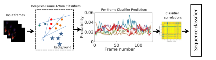
Figure 1: Internals of our correlation pooling scheme. Each video frame passes through a pre-trained set of classifiers, and their classification scores are extracted. The temporal evolution of these scores (third block above) are pooled via our correlation scheme to generate our TCP descriptor, which is then used as the action descriptor for the video.

3.3 Temporal Correlation Pooling

Using the notation defined above, let $S=\langle f_{1},f_{2},\ldots,f_{n}\rangle$ denote a sequence of frames and let $p_{m}(f_{i})$ denote the confidence that a classifier trained for the $m$-th action class predicts $f_{i}$ to belong to class $\ell_{m}$. Further, we assume that the scores $p_{m}(f_{i})$ are normalized, so that $\sum_{m=1}^{M}p_{m}(f_{i})=1,\forall i\in[n]$. Let $\bm{\alpha}^{m}=\left(\alpha^{m}_{1},\alpha^{m}_{2},\ldots,\alpha^{m}_{n}\right)$ be a given vector of weights, where each $\alpha^{m}_{i}\geq 0$ and $\sum_{i=1}^{n}\alpha^{m}_{i}=1$. Then

$$\bm{t}_{m} =\left[\alpha^{m}_{1}p_{m}(f_{1}),\alpha^{m}_{2}p_{m}(f_{2}),\ldots,\alpha^{m}_{n}p_{m}(f_{n})\right]$$ (1)

$$\triangleq\bm{\alpha}^{m}\circ p_{m}(S),$$ (2)

denotes the temporal evolution of the weighted confidence of the $m$-th classifier for the frames in the sequence $S$. We call $\bm{t}_{m}$ a feature trajectory. The weights $\bm{\alpha}$ give different priority to the classifier confidences across time, and is useful when there exists prior information that certain actions happen mostly at some specific regions of a sequence (e.g., beginning/middle/end). We define our temporal correlation pooling action descriptor as $\operatorname*{TCP}:\mathbb{R}^{M\times n}\times\mathbb{R}^{M\times n}\rightarrow\delta_{+}^{M}$, the $jk$-th entry of which is given by:

$$\operatorname*{TCP}(\bm{t}_{j},\bm{t}_{k})=\sum_{i=1}^{n}\alpha_{i}^{j}\alpha_{i}^{k}p_{j}(f_{i})p_{k}(f_{i})=\bm{t}_{j}^{T}\bm{t}_{k},$$ (3)

and captures the similarity between two such feature trajectories $\bm{t}_{j}$ and $\bm{t}_{k}$ from classifiers $p_{j}$ and $p_{k}$, respectively. It is clear that such a similarity computes the co-activations of the classifier scores over the sequence, and thus the co-occurrences of various activities. If $T\in\mathbb{R}^{M\times n}$ is a matrix whose $m$-th row is $\bm{t}_{m}$, then taking into account the auto-correlation nature of TCP, we also define $\operatorname*{TCP}(T)$ in matrix form as:

$$\operatorname*{TCP}(T)=TT^{T}\in\delta_{+}^{M},$$ (4)

where $\delta_{+}^{M}$ is the space of $M\times M$ symmetric positive semi-definite matrices. Note that, we do not center each $\bm{t}_{m}$ to the mean, as is typically done when computing correlation matrices. As a result, the $m$-th diagonal entry of $\operatorname*{TCP}(T)$ is given by:

$$\operatorname*{TCP}(\bm{t}_{m},\bm{t}_{m})=\sum_{i=1}^{n}\left(\alpha_{i}^{m}\right)^{2}p_{m}^{2}(f_{i})\leq\sum_{i=1}^{n}\alpha^{m}_{i}p_{m}(f_{i}),$$ (5)

which is the average of classifier scores, (when the $\alpha_{i}$’s are all set to $1/n$, this reduces to the popular average pooling scheme). Thus, in essence the diagonal entries of TCP captures a lower bound to the first-order statistics. In the sequel, we propose to use $\operatorname*{TCP}(T)$ as our action descriptor. Our full pipeline is depicted in Figure 1.

The basic TCP scheme described above has some shortcomings: (i) it only captures second-order temporal correlations, while higher-order may be more effective, (ii) the TCP matrix will be rank-deficient if the number of frames is less than the number of action classes (which poses difficulties when using Riemannian geometric methods on them Pennec et al. (2006)), and (iii) the size of TCP is quadratic in the number of classes, thus scaling them to large feature vectors may be difficult. We address each of these issues in detail below, thereby improving the representational power of the basic TCP scheme.

3.4 Kernelized Correlation Pooling

From (3), it is easy to see that $\operatorname*{TCP}$ is a symmetric positive semi-definite matrix produced by an inner product between feature trajectories $\bm{t}$. It is well-known that using non-linear feature maps may better capture the complex dependencies in data, leading to superior performance Vedaldi and Zisserman (2012). To this end, we propose to embed the TCP inner products into a reproducing kernel Hilbert space (RKHS) via the kernel trick. Mathematically, we rewrite $\operatorname*{TCP}$ in (3) to kernelized correlation pooling ($\operatorname*{KCP}$), where

$$\operatorname*{KCP}(\bm{t}_{j},\bm{t}_{k})=\sum_{i=1}^{n}\psi\left(\alpha_{i}^{j}p_{j}(f_{i})-\alpha^{k}_{i}p_{k}(f_{i})\right),$$ (6)

where $\psi(x-y)$ is a suitable non-linear positive definite function. Such a reformulation brings possibilities of incorporating rich non-linearities to capture the similarities between feature trajectories. In the sequel, we use the RBF kernel

$$\psi(x-y)=\exp(-\gamma\left\|{x-y}\right\|_{2}^{2}),$$ (7)

with a suitable choice of the bandwidth parameter $\gamma$.

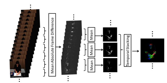
Figure 2: Schematic illustration of the steps involved in generating our SMAID images. We first convert the frames to gray-images, which are then differenced (second frame stack). These difference images are averaged to generate MAID images (third stack), which are then stacked across channels to generate SMAID.

3.5 Block-Diagonal Kernelized Correlation Pooling

While, the above discussion assumed KCP is built on classifier scores, in this section, we extend it to work with any sequence of temporal features. Unfortunately, such an extension is not straightforward, because the size of KCP is quadratic in the feature size. For example, for a typical action recognition dataset, if we use the output of the last fully-connected FC8 layer (assuming a VGG/Alexnet model) and the number of action classes is 101 (used in UCF101), then KCP given a 5151-dimensional descriptor (ignoring SPD symmetry). However, extending this setup to use intermediate layer features say from FC6 or FC7 , which are 4096-dimensional, will result in KCP descriptor size of about 8 million dimensions, posing significant storage and computational difficulties. In this section, we propose a simple workaround for this problem via a KCP approximation, termed block-diagonal kernelized correlation pooling (BKCP).

In a nutshell, our main idea of the BKCP approximation is to reduce a full KCP matrix computed over all the feature dimensions into a block-diagonalized KCP, where each diagonal block of KCP captures the second-order correlations between only a subset of the features. Given that we could treat each block-diagonal of such a matrix as an independent KCP, we could scale the size of BKCP linearly in the feature size. On the downside, we ignore some correlations that could be important. To accommodate this, we repeat this BKCP construction process several times after randomly permuting the feature indexes. Such a scheme is reminiscent of the popular product quantization techniques Jegou et al. (2011) and model averaging schemes Hoeting et al. (1999).

Mathematically, suppose $\theta(f_{i})\in\mathbb{R}^{d},i\in[{n}]$ represents features from some layer of a CNN for frames $f_{i}$. Further, let $\Theta\in\mathbb{R}^{d\times n}$ be a feature trajectory matrix built on $\theta(f_{i})$ such that the $k$-th row $\Theta_{k}$ is given by $\theta_{k}(f_{i}),i=1,2,\cdots n$, which is the $k$-th feature trajectory. BKCP aims to quantize each $\theta(f_{i})$ into the Cartesian product of several smaller features (in distinct sub-dimensions) and then compute the kernelized correlation matrix on such sub-vectors. That is, let $\theta(f_{i})\in\mathbb{R}^{p}\times\mathbb{R}^{p}\times\cdots d/p\text{ times}$. Suppose, we randomly (jointly) permute the dimensions of the feature trajectories using a permutation matrix $\pi\in\Pi\subset\mathcal{P}$, where $\mathcal{P}$ is the set of all $d\times d$ permutation matrices, and we denote this shuffling as $\pi\circ\theta(f_{i})=\pi(\theta)(f_{i})$. Let $\pi(\theta)(f_{i})^{(p(k-1)+1:kp)}\in\mathbb{R}^{p}$, ($k\in[{d/p}]$), denote such a sub-vector of $p$ dimensions of $\pi(\theta)(f_{i})$ starting at dimension $p(k-1)+1$. Then, $\forall u,v\in[{p(k-1)+1,pk}]$, we define the Block KCP (BKCP) approximation to $\operatorname*{KCP}$ for the block at $(p(k-1)+1,p(k-1)+1)$ extending to $(pk,pk)$ in KCP as:

$$\operatorname{BKCP}^{p(k-1)+1:pk}_{\pi}(\Theta_{u},\Theta_{v})=$$

$$\qquad\qquad\sum_{i=1}^{n}\exp\left(-\gamma\left\|{\pi(\theta)_{u}(f_{i})-\pi(\theta)_{v}(f_{i})}\right\|_{2}^{2}\right),$$ (8)

where we have substituted the RBF kernel for KCP as described in the last section and the notation $\pi(\theta)_{u}(f_{i})$ denote the $ui$-th entry of $\Theta$ after permuting its rows by $\pi$. We extend this definition to cover all such permutations of dimensions, and we define the approximation to KCP as:

$$\operatorname{BKCP}^{p(k-1)+1:pk}(\Theta_{u},\Theta_{v})=$$

$$\qquad\qquad\frac{1}{|\Pi|}\sum_{\forall\pi\in\Pi}\operatorname{BKCP}_{\pi}^{p(k-1)+1:pk}(\Theta_{u},\Theta_{v}).$$ (9)

In words, the steps for constructing BKCP descriptors are as follows. Suppose, we use $d$-dimensional features for every frame (i.e., there are $d$ rows in the feature trajectory matrix $\Theta$). In BKCP, first we select a permutation $\pi\in\Pi$, and permute all the rows of $\Theta$ using $\pi$. Then, we compute KCP on each disjoint set of $p$-dimensional blocks (sub-vectors or contiguous set of rows of the permuted $\Theta$). For example, the first set will have features from rows $1$ to $p$; for which we compute the KCP thereby capturing correlations between $1$ to $p$ feature dimensions, resulting in a KCP matrix of size $p\times p$. This KCP matrix is equal to some block in the matrix produced if computing KCP on all $d$ of $\Theta$; however this could be prohibitive if $d$ is large. Similarly, we compute the KCP block for rows from $p+1$ to $2p$, and so forth. We repeat this process for all $\pi\in\Pi$. The goal of selecting different permutations is to ensure that BKCP covers a large set of inter-dimensional feature correlations of the original $d\times d$ KCP matrix. Using the above procedure, we would generate $|\Pi|d/p$ KCP blocks. Finally, these KCP blocks from different permutations are averaged to generate $d/p$ KCPs, which forms the BKCP descriptor. Specifically, if we use $|\Pi|$ permutations, then the first block of BKCP will be the average of all $|\Pi|$ KCP blocks formed from dimensions $1$ to $p$, the second BKCP block will be the average of all KCPs computed on dimensions $p+1$ to $2p$, etc.

This sort of BKCP construction allows creating $d/p$ KCP matrices, which is a better approximation than averaging all KCP blocks together. The latter is not a useful idea because in that case feature correlations captured in each KCP block will be lost (due to averaging a large number of KCPs), and thus performance may degrade. The same happens if we use a very large number of permutations, in which case it is straightforward to show that all the $d/p$ averaged KCP blocks will converge to the same matrix – which is also not useful a representation. We empirically observe this effect in Figures 6(a), 6(b), and 6(c), for CNN features. Empirically, we see that more than 8 permutations will start deteriorating the action recognition accuracy.

From an efficiency standpoint, assuming $d$-dimensional features, KCP as defined in (6) will have a size $d(d-1)/2$, while BKCP will have a size $d(p-1)/2$ (as each block of BKCP is symmetric) which for appropriately chosen and fixed $p$ blocks scales linearly with $d$. Note that we fix the permutation set $\Pi$ for all sequences in a dataset to make sure the BKCP descriptors are comparable.

4 Computational Complexity

Using the notation defined in the previous sections, for a sequence of $n$ frames, represented by $M$ dimensional vectors, the cost of computing the TCP and the KCP descriptors is $\mathcal{O}(M^{2}n)$. As for the BKCP descriptor, assuming $d$-dimensional features for every frame, $|\Pi|$ number of permutations, and using a sub-vector dimension of $p$ (then we have $d/p$ feature blocks), the cost of computing BKCP is $\mathcal{O}(|\Pi|pdn)$. Using suitable values of $\Pi$ and $p$, the cost can be reduced significantly in comparison to finding the full $d\times d$ TCP descriptor. Note that, a naïve compution of TCP using a $d\times n$ feature matrix costs $d^{2}n$ time. Choosing $\Pi$ and $p$ wisely, BKCP computations can be made significantly cheaper. For example, in our experiments, we typically use $d=4096$, $|\Pi|=8$ and $p=16$, resulting in BKCP which is 32$\times$ faster. As noted above, generating and storing the TCP descriptors for the full feature matrix is a practical concern as well.

5 SMAID Image Representations

Success of any pooling scheme depends on the quality of the features (or classifier scores) used. This is because, more noise in the features (or predictions) leads to diluting the feature correlations. While, the two stream model is popular and is empirically seen to be effective, it discards the coupling between optical flow and appearance streams. For example, in Feichtenhofer et al. (2016b), a fusion of intermediate CNN layers is proposed, where the pooling between flow and RGB streams are accounted for earlier than the last layer. Such a fusion synchronizes the two disparate feature maps and allows for joint inference at the last layer. In this section, we propose a much cheaper fusion scheme using differences of frames, that approximates flow and appearance.

For a sub-sequence $S_{\tau+1:\tau+T}=\langle f_{\tau+1},\ldots,f_{\tau+\zeta}\rangle\subseteq S$ containing $\zeta$ consecutive frames, we define the mean absolute image difference (MAID) representation of $S_{\tau+1:\tau+\zeta}$ as:

$$\operatorname*{MAID}(S_{\tau+1:\tau+\zeta})=\frac{1}{\zeta-1}\sum_{j=2}^{\zeta}\left|{f_{\tau+j}-f_{\tau+j-1}}\right|.$$ (10)

As is clear, such a representation aggregates small motions over $\zeta$ consecutive frames and summarizes them in a single object with the same dimensionality as a single frame. However, such a representation loses the long-term temporal evolution of actions; to circumvent this we stack several such MAID images corresponding to consecutive non-overlapping sub-sequences as separate image channels. That is, suppose $S^{\prime}=S_{\tau+1:\tau+\beta\zeta}$ is a subsequence of $S$ containing $\beta\zeta$ frames. Then, we define our Stacked MAID (SMAID) representation as:

$$\operatorname*{SMAID}(S^{\prime})=\operatorname*{\bigotimes}_{j=1}^{\beta}\operatorname*{MAID}(S_{\tau+(j-1)\zeta+1:\tau+j\zeta}),$$ (11)

where the operator $\operatorname*{\bigotimes}$ represents stacking $\operatorname*{MAID}$ images into the third mode of a 3D tensor. To restrict the SMAID cross-channels to only allow temporal evolution of the actions, we reduce the original color images to gray-scale MAID images before stacking them. The overall SMAID pipeline is depicted in Figure 2. See Figure 8 and Figure 9 for more SMAID illustrations. As our representation only uses frame differences and averaging (as against, for example, the fusion scheme in Feichtenhofer et al. (2016b) that needs each frame to be passed through a CNN), our scheme is computationally much cheaper. For example, differencing two frames say of size 256$\times$ 256, takes slightly less than a milli-second in Matlab on a single core desktop.

Next, this SMAID image representation is fed to a three-stream CNN; consisting of separate streams for appearance, flow, and SMAID frames. Due to the demonstrated performance benefits, we chose a 16-layer VGG network Chatfield et al. (2014), pre-trained on the Imagenet dataset, to form the CNN classifiers for the individual data streams. A schematic illustration of our full pipeline is depicted in Figure 3.

6 Classification on the Riemannian Manifold

Now that, we have provided all the details for generating a second-order action descriptor for a given video sequence, let us move on to algorithms for classifying SPD matrices in an SVM setup. Our overall classification pipeline is depicted in Figure 3. As is clear, the kernelized correlation matrices are symmetric positive definite (SPD) objects themselves; each sequence generating one such object. It is well-known that these matrices belong to the strict interior of the cone of positive semi-definite (PSD) matrices. While, PSD can be treated as objects in Euclidean space under the natural Frobenius norm, it is often found that resorting to a non-linear geometry on SPD matrices can avoid unlikely or impossible outcomes (such as, for example, nearest neighbors to an SPD matrix is restricted to be only SPD matrices, instead of PSD), thereby improving application performance Pennec et al. (2006); Arsigny et al. (2006). Typically, this non-linear geometry is imposed via the respective similarity measure used to compare SPD matrices. Among the commonly used such measures Pennec et al. (2006); Cherian et al. (2013); Arsigny et al. (2006), we will be exploring two, namely (i) the Log-Euclidean metric Arsigny et al. (2006) and (ii) the Jensen-Bregman logdet divergence Cherian et al. (2013), as they are known to induce valid Mercer kernels on SPD matrices. We detail each of these measures and their respective kernels below.

6.1 Log-Euclidean Metric

For two KCPs $C_{1},C_{2}\in\delta_{++}^{d}$, the Log-Euclidean distance between them is given by:

$$\operatorname{dist}_{LE}(C_{1},C_{2})=\left\|{\operatorname*{Log}{C_{1}}-\operatorname*{Log}{C_{2}}}\right\|_{F},$$ (12)

where $\operatorname*{Log}$ is the matrix logarithm, which makes an isomorphic mapping between an SPD matrix $C$ and a symmetric matrix $\operatorname*{Log}{C}$, the latter uses the Euclidean geometry and thus similarity could be computed using the standard Frobenius norm. An advantage of using $\operatorname{dist}_{LE}$ is that it decouples the constituent matrices, such that the $\operatorname*{Log}{}$ operator could be applied during data pre-processing, after which evaluating the similarity involves only computing Euclidean distances, which can be done very fast. However, gradients of $\operatorname*{Log}{}$ is an infinite series Arsigny et al. (2006), making end-to-end learning difficult. An RBF kernel using the Log-Euclidean metric for SVM classification is introduced in Li et al. (2013) and has the following form:

$$\operatorname{K}_{LE}(C_{1},C_{2})=\exp\left(-\xi\operatorname{dist}_{LE}(C_{1},C_{2})^{2}\right),$$ (13)

where $\xi$ is a bandwidth parameter. Note that, the Log-Euclidean kernel can be viewed as the limit of the popular power-normalization strategy, which is known to combat burstiness Jégou et al. (2009), i.e., certain classifiers firing more frequently than others. In addition, the Log-Euclidean kernel can be directly applied to each block of our BKCP descriptor separately, thus making the scheme efficient (as otherwise one needs to compute the singular values of a very large KCP matrix).

6.2 Jensen-Bregman Log-Det Divergence

Another popular similarity measure on SPD matrices is the recent Jensen-Bregman Log-Det divergence (JBLD) Cherian et al. (2013) (also called Stein divergence Sra (2011)), which for two KCPs $C_{1}$ and $C_{2}$ has the following form:

$$\operatorname{dist}_{S}(C_{1},C_{2})=\operatorname*{log\det}\left(\frac{C_{1}+C_{2}}{2}\right)-\frac{1}{2}\operatorname*{log\det}{\left(C_{1}C_{2}\right)}.$$ (14)

In contrast to the Log-Euclidean metric, JBLD is not a Riemmannian measure, instead is a symmetric Bregman divergence which captures the information divergence between a function and its first-order Taylor approximation (the function is $-\operatorname*{log\det}$ in this case). It is related to the Bhattacharya distance Jebara and Kondor (2003) between two zero mean Gaussian distributions with covariances $C_{1}$ and $C_{2}$. In contrast to the Log-Euclidean metric that needs to compute the matrix logarithm of the constituent matrices, JBLD needs only the matrix determinant, which is computationally cheaper. In Sra (2011), a kernel is defined using JBLD as defined below:

$$\operatorname{K}_{S}(C_{1},C_{2}) =\exp\left(-\xi\operatorname{dist}_{S}(C_{1},C_{2})\right),$$ (15)

$$\forall\xi \in\left\{\frac{k}{2},k=1,\cdots,d-1\right\}\cup\left[d,\infty\right),$$

where the bandwidth parameter $\xi$ is defined only for certain values. In contrast to the Log-Euclidean metric, JBLD offers computationally cheaper gradients, as will be explored in the next section.

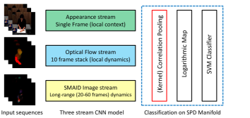
Figure 3: An illustration of our overall CNN architecture and our pooling scheme. We use a non-linear feature pooling scheme based on Riemannian geometry to generate an action descriptor.

7 End-to-End CNN Training

In this section, we explore an end-to-end CNN architecture that learns the action descriptors and the classifiers jointly via gradient back-propagation. As is the case with any end-to-end CNN models, the main challenge in designing this model is to define the gradients of the objective with respect to the inputs. There have been several previous attempts at implementing end-to-end second-order CNN models. In Ionescu et al. (2015), the Log-Euclidean metric is used to define the CNN loss function. While computing gradients of this metric is challenging (as $\operatorname*{Log}{}$ involves an SVD operation which by itself is expensive when it needs to be done a large number of times within optimization schemes such as stochastic gradient descent), it also demands flattening of the matrix, leading to very large fully-connected layers that scales quadratically with the number of data classes. In Huang and Van Gool (2017), a CNN model that takes SPD matrices as input is presented. Another recent attempt ( Yu and Salzmann (2017)) is to map the second-order SPD matrices into a lower-dimensional SPD manifold through parametric second-order transformation, followed by parametric vectorization. However, such parametric transforms also introduce additional capacity to the networks that needs to be learned. In contrast to all these methods, we propose to directly use second-order similarity measures to define loss functions, which as we show below leads to simple and straightforward gradient formulations, without the need for introducing any new parameters into the framework. We explore two such loss functions, namely (i) using the Jensen-Bregman Logdet Divergence as introduced in (14), and (ii) using the simple Frobenius norm.

7.1 End-to-End Learning Using Stein Divergence

Suppose $T\in\mathbb{R}^{M\times n}$ denotes the CNN feature trajectories (from say the FC8 layer of a standard VGG/ Alexnet model) for $n$ frames in a sequence and $M$ action classes. Further, let $Y$ denote an $M\times M$ diagonal ground-truth label matrix for a ground-truth label $\ell$ associated with $T$; the $jj$-th diagonal entry of $Y$ is defined as

$$Y_{jj}=\begin{cases}1/\left(1+(M-1)\epsilon\right),\qquad\text{if }j=\ell_{i}\\ \epsilon/\left(1+(M-1)\epsilon\right),\qquad\forall j\neq\ell_{i}\end{cases}$$ (16)

where we assume $\epsilon$ is a small number (say $10^{-5}$ used in our experiments). This encoding of ground truth class label is similar to the standard one-hot encoding used with a softmax cross-entropy loss framework. However, given that we propose to use similarity measures defined on SPD matrices in our loss, we cast the label in a matrix form and use a small $\epsilon$ regularization to make sure this matrix SPD.

Suppose, we have a training set consisting of such sequences of CNN feature trajectories $\mathcal{T}=\left\{T^{1},T^{2},\cdots T^{N}\right\}$ for video sequences in $\mathcal{S}$ and their associated ground-truth encoded matrices $\mathcal{Y}=\left\{Y^{1},Y^{2},\cdots,Y^{N}\right\}$. Then using the JBLD measure introduced in (14), we define the TCP CNN loss as:

$$\operatorname{loss}(\mathcal{T},\mathcal{Y}):=\sum_{\forall(T,Y)\in\mathcal{T}\times\mathcal{Y}}\bigg{[}\log\det{\left(\frac{Y+\operatorname*{TCP}(T)}{2}\right)}$$

$$\qquad\qquad\quad-\frac{1}{2}\log\det{Y}-\frac{1}{2}\log\det{\left(\operatorname*{TCP}(T)\right)}\bigg{]},$$ (17)

$$\text{\quad where }\operatorname*{TCP}(T)=\frac{1}{n}T{T}^{T}.$$

For implementing back-propagation, we need the gradient of $\operatorname{loss}$ with respect to a data matrix $T$ (with associated label matrix $Y$) and is as follows:

$$\frac{\partial\operatorname{loss}(T,Y)}{\partial T}=\frac{2}{n}\left\{\bigg{(}\operatorname*{TCP}(T)\!+\!Y\bigg{)}^{-1}\!\!\!\!\!\!\!-\frac{1}{2}\operatorname*{TCP}(T)^{-1}\right\}T.$$ (18)

7.2 End-to-End Learning Using Frobenius Norm

A difficulty usually encountered with the gradient defined in (18) is the need to compute the matrix inverse, which is expensive and will also sometimes lead to numerical instability. Thus, we also propose to use the matrix Frobenius norm to define the CNN loss, which avoids these issues. As this loss will not require the label matrix $Y$ to be SPD, we assume $\epsilon=0$ in this case in (16). Reusing the notations from the last section, we define the new loss as:

$$\operatorname{loss}(\mathcal{T},\mathcal{Y}):=\sum_{\forall(T,Y)\in\mathcal{T}\times\mathcal{Y}}\left\|{\operatorname*{TCP}(T)-Y}\right\|_{F}^{2},$$ (19)

and the respective gradient with respect to a data matrix $T$ has the form:

$$\frac{\partial\operatorname{loss}(T,Y)}{\partial T}=\frac{2}{n}\bigg{(}\operatorname*{TCP}(T)-Y\bigg{)}T$$ (20)

Empirically, it is observed that using the softmax output of the FC8 CNN layer for constructing the above losses leads to better convergence of the models.

8 Experiments

In this section, we evaluate the usefulness of our proposed framework on four datasets. Two of these datasets, namely the MPII Cooking activities dataset Rohrbach et al. (2012), and the JHMDB dataset Jhuang et al. (2013), are standard fine-grained benchmarks. We also provide evaluations on HMDB and UCF101 datasets, which are standard benchmarks with fine-grained as well as coarse action categories. As for the CNN architecture, we report results using Alexnet Krizhevsky et al. (2012), VGG-16 Chatfield et al. (2014), and ResNet-152 He et al. (2016), demonstrating that the benefits showcased by our representations are CNN architecture agnostic. Below, we provide details of these datasets, data preparations, evaluation protocols, and our results. Later, in Section 9.8, we provide experimental results on the large-scale Kinetics-600 dataset.

8.1 Datasets

MPII Cooking Activities Dataset Rohrbach et al. (2012):

This dataset consists of high-resolution videos of cooking activities captured by a static camera. The videos are of 14 different people cooking various dishes and consists of 64 distinct activities spread across 3748 video clips and one background activity (1861 clips). There are over 800K frames and the activities range from coarse subject motions such as moving from X to Y, opening refrigerator, etc., to fine-grained actions such as peel, slice, washing hands, cut ends, cut apart, etc. This dataset is challenging due to several reasons, namely (i) the classes are very unbalanced – there are certain activities that have only about 1K frames over the entire dataset, (ii) there is significant intra-class variability as the participants are only asked to prepare one of a set of 14 dishes and allowed to cook in their own styles, and (iii) there are no annotations of objects in the scene, and the tools used for actions are very small (such as spice folder, knife, etc.) and thus hard to detect.

HMDB Dataset Kuehne et al. (2011):

It consists of 6766 videos from 51 different action categories, mostly web videos of low resolution and quality. Each video clip is a few seconds long. The actions in these clips vary significantly in lighting, and viewpoints, and may have significant camera motions making the action recognition task challenging. The dataset includes videos that are not person centered and the actor may undergo occlusions as well.

JHMDB Dataset Jhuang et al. (2013):

This dataset is a subset (960 videos) of the HMDB dataset consisting of 21 actions, but contains videos for which the human limbs can be clearly identified. It was primarily designed for action recognition using human poses. The dataset contains action categories such as brush hair,  pick, pour, push, etc.

UCF101 Dataset Soomro et al. (2012):

This dataset contains 13320 videos spread in 101 action categories. The dataset is different from the above ones in that in addition to several of the categories found in HMDB dataset, it also contains videos on sports activities; such videos usually have strong camera motions, long shots (and thereby person occupying very small portions of the scene), and fast actions. The clips in this dataset are also of low resolution and of web quality. A few illustrative actions in this dataset are cartwheel, somersault, kayaking, Tennis swing, etc. and also includes non-sports actions such as apply eye makeup, brushing teeth, etc., similar to the ones in the HMDB dataset.

Evaluation Protocols:

Following the standard protocols, we use mean average precision over 7-fold cross-validation on the MPII dataset. Other datasets use mean average accuracy on 3-splits. For the former, we use the evaluation code published with the dataset.

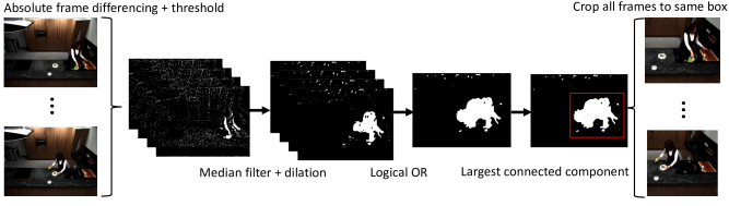
Figure 4: Preprocessing pipeline for the MPII dataset. Our goal is to generate the smallest bounding box (for the full clip) that will contain the moving parts in the video; subsequently cropping the high-resolution frames to this box. As the crop box is computed for all frames, the background is kept constant after the crop, while the relevant action dynamics are contained in this box.

8.2 Preprocessing

The original MPII cooking videos are very high resolution (1624$\times$1224), however the actions happen only at certain parts of the scene. Given that such full resolution frames cannot be directly used to train the CNNs, and resizing the frames to a CNN input resolution might reduce the number of pixels belonging to the actions, an attention mechanism is important to crop the frames around regions around actions. Further, we would also want to use the fact that the camera is static (which will be useful to compute SMAID images). Thus, we use morphological operations to compute these action regions, as detailed below. We found that using a person detector (such as using a faster-RCNN Ren et al. (2015)) per frame – that returns a person bounding box, and then finding a crop box for the sequence that is a rectangular hull of all the frame level boxes – will lead to similar results.

As alluded to above, instead of using a faster RCNN for finding the crop box that needs every frame to be passed through a CNN, we resort to a simple set of morphological operations, that are computationally much cheaper and produces the same result. The preprocessing pipeline is illustrated in Figure 4. Specifically, for every sequence, we first convert the frames to half their sizes, followed by frame-differencing that produces appearance blobs corresponding to the moving parts (mostly parts of human body, such as hands). We then dilate these blobs using a $11\times 11$ dilation filter to capture details surrounding them. This is followed by Gaussian smoothing and connected components analysis to find blobs connected to each other. The connected components are converted to binary masks, and are merged with such components across frames in the sequence (logical OR). For example, in the case when a person moves from say X to Y in the sequence, our scheme results in a binary mask of the person per frame, and such masks are merged (as they will be connected due to the neighborhood) across frames, resulting in one large blob for the motion from X to Y. We then use the largest such merged binary blob and crop the sequence to a box containing this blob. The cropped frames are then resized such that their shorter side is 256 pixels, to be used for training the CNNs. We use these resized frames for computing optical flow using the TVL1 OpenCV implementation. Each flow image is then thresholded to $\pm$ 20 pixels, rescaled to 0–255, and saved as a JPEG image for storage efficiency as described in Simonyan and Zisserman (2014).

For the JHMDB dataset, we use the RGB frames resized such that the shorter side is 256 pixels, and compute optical flow on them directly using the same scheme described above. For the UCF101 and HMDB datasets, we use the pre-processed frames and flow images publicly shared as part of two-stream fusion implementation Feichtenhofer et al. (2016b).

8.3 Experiment Setup

All the three CNN streams (RGB, Flow, and SMAID) are trained separately. Among the end-to-end CNN loss variants (Frobenius norm versus Stein divergence), we use the Frobenius norm due to its superior speed and numerical stability. We found that the performance of Frobenius norm is very similar to the standard softmax cross-entropy loss. We use sub-sequences of 30 frames for computing the correlation matrices in the end-to-end setup. Given a fixed CNN batch size (number of frames), we could not use more frames per sequence, as this limits the number of sequences that could be used in a training batch, and thus restricting the batch diversity (different action classes in the same batch). Less diverse such batches are known to impact convergence. Once the CNNs are trained, we use a forward pass to compute per-frame features, which is then used to generate sequence level TCP descriptors and variants. These descriptors are then used in a Riemannian geometry based SVM classification framework, thus utilizing the power of non-linear geometry. We found that this provided significantly better accuracy than just using the end-to-end learned model.

In all the experiments to follow (except for the ones analyzing the parameters for SMAID), we use the following settings. We use a VGG-16 model pre-trained on UCF101 dataset, to fine-tune the models for JHMDB, MPII Cooking activities, and the HMDB-51 datasets. As alluded to above, we use single RGB images for the RGB stream, a stack of ten consecutive optical flow images for the flow stream, and three-channel 21–45 frames summarized into SMAID images for the respective CNN stream. To train the SMAID CNN stream, we use the RGB stream of the above pre-trained model for initialization of the stream weights, which seemed to perform significantly better than learning from scratch. For fine-tuning, we used a fixed learning rate of $10^{-4}$ and a momentum of 0.9. We used the Caffe toolbox for our CNN implementations. We also applied the standard data augmentation techniques (such as mirroring) on the data inputs. For the RGB stream, the CNN iterations usually converged in about 20k iterations, the optical flow stream 40–60k iterations, and about 70k iterations for the SMAID stream. We also followed the same procedure for the ResNet-152 model by fine-tuning on a UCF101 pre-trained model.

During testing, predictions from each of the three streams (output of FC8 layer in VGG-16 and the FC layer in ResNet-152), are normalized to be in $[0,1]$ after subtracting the minimum value, and are aggregated at the sequence level, kernelized (using a $\gamma=1$), and later vectorized after taking the matrix logarithm. For the MPII dataset, we used the provided training and validation sets. For JHMDB, we used 95% of the training set to fine-tune CNNs, 5% as validation. For the UCF101 dataset, we directly used the pre-trained CNN models for the RGB and FLOW streams. For HMDB dataset, we trained our three streams by fine-tuning those used for UCF101. Note that while we use the pre-trained models from Feichtenhofer et al. (2016b), we do not use their fusion architecture in our evaluations. Instead, we use the setup in Simonyan and Zisserman (2014), but using a VGG-16 or ResNet-152 model.

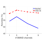
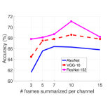
Figure 5: Evaluation of the effect of increasing number of SMAID channels (keeping number of frames per channel fixed at 7) and increasing number of frames per channel (while keeping the number of channels fixed at 3) on the UCF101 dataset split-1 using Alexnet, VGG-16, and ResNet-152 architectures. Alexnet and VGG-16 was trained from scratch, while ResNet-152 was fine-tuned from an ImageNet pre-trained model.

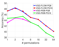
(a) MPII-VGG16

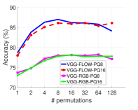
(b) UCF101-VGG16

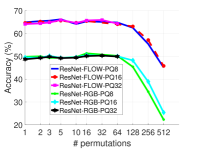
(c) HMDB-ResNet-152

Figure 6: Evaluation of the effect increasing the number of BKCP sub-vector dimensions and the size of the permutation set when constructing BKCP descriptors. Figure 6(a) shows the results on the MPII dataset using VGG16 fc6 features for sub-vector dimensionality 8 and 16 for optical flow and RGB streams. Figure 6(b) shows the same for the UCF101 dataset, and Figure 6(c) shows the results using ResNet-152 pool5 features on the HMDB dataset. The plots are generated after averaging the performance of 5 different random permutation sets for each dataset. The standard deviation of the performances is found to be less than 1% on all the datasets. Best viewed in color.

8.4 SMAID Image Parameters

As noted earlier, SMAID images summarize long-range actions into a compact image representation. There are two parameters for this representation: (i) number of frames that can be effectively summarized in a SMAID channel ($\zeta$ in (10)), and (ii) number of channels that can be stacked to capture the dynamics ($\beta$ in (11)). Depending on the sequences, too many frame differences for (i) might result in a cluttered image that may not be useful for learning actions, while too less frames might lead to very sparse images. For (ii), while a 3-channel stack will render the SMAID as equivalent of an RGB image and thus RGB based CNN architectures could be used, higher-number of channels will require redesigning the network, and also leading to more CNN parameters. See Figure 9 for example frames from the UCF101 dataset for various number of frames encoded per channel in a 3-channel SMAID setup.

To understand the effect of these parameters, we progressively increased (i) and (ii) on a subset of the UCF101 split-1 training set containing videos that had limited camera motion, and evaluated on a small validation subset. The plots use Alexnet, VGG16, and ResNet-152 models, the former two trained from scratch, while the ResNet-152 model is trained from an ImageNet pre-trained model (as training from scratch takes too long due to the depth of the network). In Figure 5, we plot the classification accuracy. The plots reveal that higher number of frames per channel in SMAID leads to performance improvements, but with more than a certain number (for example, 7 for Alexnet, about 10 for VGG and ResNet), the performance drops, perhaps because of increasing clutter (see Figure 9). On the other hand, with increasing number of SMAID channels (beyond three), the performance is seen to decrease for all the models, which is surprising. We think this behavior is perhaps because of the typical network structure that we use, which is designed for RGB images, and is thus inadequate for a SMAID image with more than three channels. In the sequel, we use a 3-channel SMAID stack, with 15 frames per channel for the UCF101 dataset. We chose 15 frames instead of 10 frames as suggested from Figure 5 because the difference between 7 or 10 frames per channel and 15 frames per channel in Figure 5 is only about 1%. Further, 15 frames per channel gives a longer 45 frames summarization of the sequence than say 30 frame-summarization using 10 frames per channel. For the ResNet-152 model, we use 10 frames per channel as the difference to 15 frames per channel is more than 5%. As it is computationally expensive to cross-validate the best SMAID parameters for all our datasets, we repeated these parameter search experiments only for a few discrete settings and choose the best results in our subsequent experiments. We found that the same UCF101 parameters works well for the HMDB dataset. However, we found 7 frames per channel work best for MPII cooking activities and JHMDB datasets. With these configurations, each SMAID image captures subsequences of 45 frames in UCF101 and HMDB-51, and 21 frames in JHMDB and MPII datasets.

We would also like to point out that SMAID with only one frame-difference per channel is equivalent to some of the recent proposals described in Wang et al. (2016) and Sun and Nevatia (2014). However, as is clear from Figure 5, more frames per channel is significantly better. Further, looking back at Figure 5, a single channel SMAID is a grayscale image, similar to a motion history image Davis and Bobick (1997). However, using more channels is clearly beneficial. These two plots substantiates that the design of SMAID is better than existing frame summarization techniques based on frame differencing.

Experiment	MPII-mAP (%)	JHMDB-Avg.Acc.(%)	HMDB-Avg. Acc.(%)		UCF101-Avg. Acc. (%)
	VGG16	VGG16	VGG16	ResNet152	VGG16	ResNet152
RGB	33.9	51.5	40.9	45.4	82.0	83.1
FLOW	37.6	54.8	47.5	59.5	85.1	86.4
SMAID	35.4	61.1	41.1	42.3	72.1	70.1
RF	38.1	55.9	53.6	62.1	88.5	89.5
RS	38.4	62.0	50.1	55.5	85.5	86.7
RFS	39.5	62.6	54.4	63.5	88.8	91.0

Table 1: Sequence level comparison by directly averaging the CNN classifier outputs (not using correlation pooling) on MPII cooking dataset, JHMDB, HMDB and UCF101 (split-1). The goal of this experiment is to show the advantages afforded by the standalone SMAID representation without any correlation pooling. The results on MPII and JHMDB datasets use a VGG-16 architecture, while HMDB and UCF101 use both VGG-16 and ResNet-152 models.

8.5 Parameters for BKCP

The block-diagonal approximation for KCP has two parameters, namely (i) the length of the sub-vectors ($p$ defined in (9)) and the number of feature permutations to be tried to estimate the BKCP descriptor. For the former, as is clear, higher values of $p$ demands higher computations, while lower $p$ will ignore important correlations; in the limit $p=1$ is only the diagonal correlation matrix, which corresponds to average pooling. In Figure 6, we evaluate performance for various choices of these BKCP parameters on MPII cooking activities (Figure 6(a)), UCF101 (Figure 6(b)), and HMDB datasets (Figure 6(c)), using a VGG architecture, on the first two, and a ResNet-152 architecture on the third one. We mainly use $p=8,16$ as higher values lead to higher-dimensional descriptors (and thus are expensive, see Section 4), and also show inferior performance (Figure 6(c)). The latter observation is perhaps due to the fact that such higher dimensional sub-vectors result in mostly ill-conditioned blocks in TCP. This is because in most of our datasets, there are one average 50 to 100 frames per sequence. Given that we use the rectified features (after ReLU in the CNNs), they are mostly sparse. Both these factors result in TCP descriptors that are low-rank for higher $p$ and thus performance degrades. Thus, we find that using sub-vectors of length $p=16$ show good performance overall, and we use this configuration in our experiments to follow.

From the plots in Figures 6(a), 6(b), and 6(c), we also find that a small number of permutations (in the range of 2–8) is sufficient to get a reasonable accuracy on all the datasets, and a higher number hurts. This suggests that the CNN features are perhaps strongly localized in their dimensions, as seen in the plots for a unit permutation set size. Further, we also suspect that averaging over too many randomized cross-dimensional correlations essentially marginalizes out any useful localized cues, thereby leading to poor accuracy. To validate this, we analyzed the average variance of the TCP descriptors for increasing number of permutations. We found that the variance steadily increases for more permutations. For example, it is on average 0.31 for ResNet-152 features for a single permutation, and goes beyond 1.5 when using 32 permutations. With such large variance, the data becomes mostly noise and thus any useful representational benefits are lost – as is clear from the performance drop witnessed in Figure 6(c). Thus, we use a permutation set of size 3 for VGG and 8 for ResNet152, in our subsequent experiments.

9 Results

In this section, we provide systematic evaluations of our various schemes on the four datasets. The notation RGB, FLOW, and SMAID denote the respective frame-level features. We denote the combinations of RGB+FLOW as RF, RGB+SMAID as RS, and RGB+FLOW+SMAID as RFS, where the combinations are either averaged over their softmax CNN outputs for frame-level predictions, or their log-mapped features concatenated when using the correlation pooling schemes.

9.1 Evaluating the SMAID Representation

First, we evaluate our SMAID representation at the frame-level against alternatives such as (i) using only a single stream image model RGB and (ii) using only optical flow stream FLOW. In Table 1, we provide these results on the four datasets. As is clear, SMAID is seen to improve performance on all the datasets, while its benefits are more on the MPII and JHMDB datasets (for example, the improvements from RF to RFS are about 2% on MPII, and 8% on JHMDB) as the camera motion is absent. While, the significance of SMAID is marginal on HMDB and UCF101 datasets – that have strong camera motions – when using a VGG-16 architecture, we find that they show about 2% improvement when using a powerful ResNet-152 model, which is encouraging. We also find that RS provides strong complementarity to the RGB stream (RGB to RS is 33.9 to 38.4 on MPII, 51.5 to 62.0, 45.4 to 55.5 on HMDB, and 83.1 to 86.7 on UCF101) showing about 6-10% improvements. However, as is expected SMAID cannot replace the performance brought out by optical flow as is clear from the table.

Expt	MPII			JHMDB
	TCP	KCP	BKCP	TCP	KCP	BKCP
RGB	49.7	52.7	55.2	44.8	51.8	48.8
FLOW	55.6	60.6	61.4	56.0	61.9	66.0
SMAID	51.3	55.7	59.6	47.2	59.7	55.6
RF	60.0	64.4	65.6	59.1	61.2	70.1
RS	57.2	61.9	64.9	49.1	60.1	63.4
RFS	62.1	66.1	68.0	62.1	72.4	73.6

Table 2: Comparison of temporal correlation pooling (TCP) against KCP and BKCP variants. These results use a VGG-16 model for the two datasets. MPII results use mAP scores and JHMDB reports the mean classification accuracy. All results are on the split-1.

Expt	HMDB						UCF101
	TCP		KCP		BKCP		TCP		KCP		BKCP
	VGG	ResNet	VGG	ResNet	VGG	ResNet	VGG	ResNet	VGG	ResNet	VGG	ResNet
RGB	52.8	55.1	56.7	59.9	58.7	60.3	79.1	82.6	82.2	86.2	76.9	83.9
FLOW	45.9	59.3	53.3	65.2	57.2	65.3	83.1	86.1	86.1	88.9	83.4	88.3
SMAID	49.4	24.9	52.9	37.4	52.1	43.7	74.2	72.2	71.7	75.3	70.7	71.2
RF	57.1	63.6	65.2	69.9	68.1	69.6	86.2	91.1	87.8	94.0	87.5	92.9
RS	55.2	56.7	60.5	61.4	63.0	61.3	82.2	85.1	85.7	86.9	81.2	85.0
RFS	57.8	57.3	66.7	68.4	68.5	71.3	87.2	91.1	88.3	94.5	87.9	93.5

Table 3: Comparison of classification accuracy between TCP, KCP, and BKCP. TCP and KCP uses the outputs of FC8 layers for VGG-16 and FC layer for ResNet-152. BKCP uses FC6 layer features of VGG-16 and pool5 features of ResNet-152. All results are on the split-1.

9.2 Correlation Pooling

Next, we evaluate our correlation pooling (TCP) scheme and its kernelized variants (KCP and BKCP) on CNN features (FC8 and FC layer for VGG16 and ResNet-152 respectively for both TCP and KCP, and FC6 and pool5 of VGG16 and ResNet-152 respectively for BKCP) from the three input modalities. The results are shown in Tables 2 and 3. Comparing these results to those in Table 1, show that KCP improves sequence level performance substantially on all datasets; from 39.5% to 66.1% for RFS on MPII, from 62.6% to 72.4% on JHMDB, from 54.4% on HMDB-51 63.5 to 66.5% and 91.0% to 94.5% on UCF101. Tables 2 and 3 also show that kernelizing the temporal correlations (TCP versus KCP or BKCP) is always useful; demonstrating a consistent 5-10% improvement from its non-kernelized variant. We also find that BKCP performs better than KCP overall. This is unsurprising given that BKCP has more dimensionality, and also captures features in the CNN pipeline more closer to the input images than KCP that directly operates on the CNN classifier outputs – as a result, class confusions are more prominent in BKCP and thereby better correlation descriptors. However, for UCF101 dataset, we find that the effects are reversed almost consistently. This we suspect is due to the larger training size of this dataset – as a result the final CNN features are already very discriminative for the actions. This intuition is consistent with the results in Table 1 for UCF101, where the final frame-level average pooling accuracy is already high. However, we still find that KCP and BKCP is beneficial and improves the average pooling performance by about 2-3%.

9.3 BKCP versus Low-Rank Decomposition

Recall that BKCP is introduced as KCP descriptors turned out to be too expensive for high-dimensional CNN features. However, an alternative would be to use a low-rank decomposition, such as PCA, on these features and then apply KCP on the low-dimensional features obtained after projection onto the principal components. We explore this alternative in Table 4 on the MPII and HMDB datasets. For learning the basis, we randomly sample 1000 sequences from the respective training sets and their associated CNN features, followed by applying an SVD to find the basis. We tried various number of basis (based on the performance on a validation set) and selected 256 basis that seemed to give the best performance in terms of feature dimensionality, computational expenditure, and accuracy. As is clear from the Table 4, using PCA does provide useful lower dimensional KCP representations, however, BKCP still outperforms it. We think this is because as the basis are learned generically over a large portion of the dataset, the sequence level features when projected onto such a basis, may lose information that are perhaps subtle (and thus not captured by any principal component) and important. We see a consistent drop in performance on both RGB and FLOW streams for both the datasets.

9.4 KCP versus Fisher Vectors

In this section, we compare KCP with Fisher vector encodings, which are well-known and successful second-order representations used in a variety of vision applications, including action recognition Newell et al. (2016). In this experiment, we apply Fisher vectors on the output of the last CNN layer (as is used in for generating KCP descriptors). A first step to generate Fisher vectors is to train a Gaussian Mixture model. To this end, similar to our approach in the last section, we sampled 1000 sequences randomly from the respective training set, and used 256 Gaussians in the mixture. Once the mixture model is trained, we used the VLFeat software  to generate Fisher vector encodings for every sequence, which is then classified using a linear classifier. Our results and comparisons to exactly similar features represented using KCP descriptors is provided in Table 5. Again, as observed in the previous section, we see a significant drop in performance when using Fisher vectors against KCP on both HMDB and MPII datasets and for both FLOW and RGB modalities.

Experiment	HMDB-Avg. Acc.(%)	MPII mAP (%)
R-BKCP	52.1	55.2
F-BKCP	66.0	61.4
R-PCA	46.1	40.3
F-PCA	64.8	48.8

Table 4: Comparison of BCKP to low-rank decompositions (PCA). For the latter, we use 256 basis, and applied KCP on the resulting projected features. HMDB uses ResNet-152 pool5 features (2048D), while MPII uses VGG16 features (4096D).

Experiment	HMDB-Avg. Acc.(%)	MPII mAP (%)
R-KCP	49.9	52.7
F-KCP	65.2	60.6
R-Fisher Vec	35.9	30.4
F-Fisher Vec	48.7	38.1

Table 5: Comparison of KCP to Fisher vector encoding. We used 256 Gaussians in the Fisher vector Gaussian mixture model. HMDB and MPII datasets use the outputs of the last fully-connected layers of a ResNet-152 and VGG-16 models respectively.

9.5 KCP Classification Kernel

As reviewed in Section 6, there are popularly two SVM kernels on SPD matrices, the Stein kernel and the Log-Euclidean kernel. In Table 6, we show results comparing these two kernels on the MPII Cooking Activities and the JHMDB datasets. As is clear, either kernel performs differently and generate improvements, suggesting that it is better to cross-validate each of the kernels on the respective datasets to choose the right one. Given that the improvements produced by the log-euclidean kernel on the JHMDB dataset is significantly higher than the improvements by the Stein kernel on the MPII dataset and further noting the computational advantages as described in Section 6.1, we decided to use the log-euclidean kernel in the sequel.

Experiment	MPII	JHMDB
	KCP mAP(%)	KCP Avg.Acc.(%)
LE Kernel	66.1	72.7
Stein kernel	68.5	62.5

Table 6: Comparison of performance when using different kernels in SVM for classifying the kernelized correlation matrices over the three input modalities.

Class Name	# seq	Zhou et al. (2015)	Ours
Change temperature	27	59.26	96.30
Cut apart	97	50.52	62.89
Cut dice	40	12.50	22.50
Cut in	12	25.00	0.00
Cut off ends	27	48.15	3.70
Cut out inside	37	62.16	75.68
Cut slices	91	40.66	81.32
Cut stripes	12	25.00	16.67
Dry	26	92.31	100.00
Fill water from tap	3	100.00	66.67
Grate	19	63.16	78.95
Lid: put on	6	50.00	0.00
Lid: remove	8	87.50	0.00
Mix	5	60.00	0.00
Move from X to Y	70	72.86	75.71
Open egg	5	80.00	40.00
Open tin	7	71.43	71.43
Open/close cupboard	18	88.89	66.67
Open/close drawer	58	48.28	68.97
Open/close fridge	8	87.50	50.00
Open/close oven	1	100.00	0.00
Package X	6	83.33	16.67
Peel	64	76.56	79.69
Plug in/out	6	100.00	33.33
Pour	55	83.64	72.73
Pull out	4	100.00	25.00
Puree	12	75.00	83.33
Put in bowl	127	40.16	88.98
Put in pan/pot	28	32.14	75.00
Put on bread/dough	149	55.70	93.29
Put on cutting-board	57	63.16	45.61
Put on plate	55	30.91	70.91
Read	8	50.00	50.00
Remove from package	15	60.00	53.33
Rip open	6	66.67	0.00
Scratch off	12	58.33	0.00
Screw close	44	75.00	52.27
Screw open	45	68.89	53.33
Shake	72	73.61	83.33
Smell	16	12.50	56.25
Spice	20	80.00	55.00
Spread	12	50.00	25.00
Squeeze	18	66.67	83.33
Stamp	8	62.50	75.00
Stir	38	57.89	86.84
Strew	40	17.50	72.50
Take & put in cupboard	10	80.00	30.00
Take & put in drawer	8	62.50	12.50
Take & put in fridge	9	100.00	66.67
Take & put in oven	3	100.00	100.00
Take & put in spice holder	13	61.54	61.54
Take ingredient apart	39	48.72	43.59
Take out from cupboard	57	94.74	92.98
Take out from drawer	130	85.38	94.62
Take out from fridge	34	94.12	97.06
Take out from oven	3	100.00	0.00
Take out from spice holder	17	82.35	70.59
Taste	12	75.00	16.67
Throw in garbage	39	64.10	84.62
Unroll dough	3	100.00	100.00
Wash hands	45	55.56	37.78
Wash objects	91	96.70	86.81
Whisk	9	77.78	88.89
Wipe clean	10	80.00	20.00
Mean		62.7	70.0

Table 7: A comparison of classification accuracy per class (not mAP) on the MPII dataset against the method in Zhou et al. (2015). Our method uses KCP.

Algorithm	mAP(%)
Holistic + Pose Rohrbach et al. (2012)	57.9
Video Darwin Fernando et al. (2015b)	72.0
Interaction Part Mining Zhou et al. (2015)	72.4
P-CNN Chéron et al. (2015)	62.3
P-CNN + IDT-FV Chéron et al. (2015)	71.4
Semantic Features Zhou et al. (2014)	70.5
Hierarchical Mid-Level Actions Lan et al. (2015)	66.8
Higher-order Pooling Cherian et al. (2017b)	73.1
KCP	66.1
BKCP	68.0
BKCP + KCP	68.6
KCP + Trajectories	73.5
BKCP + Trajectories	72.4
BKCP + KCP + Trajectories	74.7

Table 8: MPII Cooking Activities (7-splits)

Algorithm	Avg. Acc. (%)
P-CNN Chéron et al. (2015)	61.1
P-CNN + IDT-FV Chéron et al. (2015)	72.2
Action Tubes Gkioxari and Malik (2015)	62.5
Stacked Fisher Vectors Peng et al. (2014)	69.03
IDT + FV Wang and Schmid (2013)	62.8
Higher-order Pooling Cherian et al. (2017b)	73.3
KCP	72.7
BKCP	72.4
BKCP + KCP	73.7
KCP + IDT-FV	74.1
BKCP + KCP + IDT-FV	77.3

Table 9: JHMBD Dataset (3-splits)

Algorithm	HMDB-51(%)		UCF101(%)
Two-stream Simonyan and Zisserman (2014)	59.4		88.0
Two-stream Fusion Feichtenhofer et al. (2016b)	69.2		93.5
TSNWang et al. (2016)	69.4		94.2
I3D (Kinetics) Carreira and Zisserman (2017)	80.2		97.9
ActionVLAD+IDT Girdhar et al. (2017)	69.8		93.6
I3D+SVMP Wang et al. (2018)	81.3		–
Kernel Rank Pool Cherian et al. (2018)	74.2		–
IDT+FV Wang and Schmid (2013)	57.2		85.9
IDT+HFV Peng et al. (2016)	61.1		87.9
TDD+IDT Wang et al. (2015)	65.9		91.5
DT+MVSV Cai et al. (2014)	55.9		83.5
Dynamic Image Bilen et al. (2016)	65.2		89.1
ST-ResNet Feichtenhofer et al. (2016a)	70.3		94.6
ST-MultiplierFeichtenhofer et al. (2017)	72.2		94.9
	VGG	ResNet	VGG	ResNet
KCP	65.8	68.7	89.1	91.0
BKCP	68.5	70.0	88.6	91.1
KCP + BKCP	67.8	71.3	89.4	93.7
KCP + IDT-FV	67.2	69.2	92.0	94.5
BKCP + IDT-FV	69.6	72.0	89.3	93.1
BKCP + KCP + IDT-FV	70.5	72.5	92.4	95.4

Table 10: Average classification accuracy (%) over 3-splits on the HMBD-51 and UCF-101 Datasets.

Action	RF	RFS
	mAP (%)	mAP (%)
Change Temperature	32.1	50.7
Dry	46.6	53.6
spice	29.4	34.9
put on cupboard	24.1	18.3

Table 11: Analysis of per-class recognition accuracy on the MPII dataset with avg. pooling when using RGB + FLOW against RGB+FLOW+SMAID.

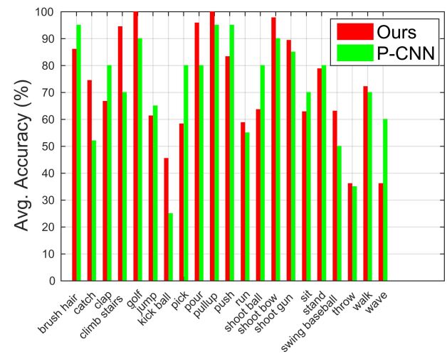
Figure 7: KCP per-class classification accuracy of sequences in the JHMDB dataset in comparison to the results in Chéron et al. (2015).

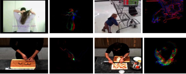
Figure 8: Qualitative SMAID and the associated appearance images from the JHMDB dataset (top) and the MPII Cooking activities dataset (bottom).

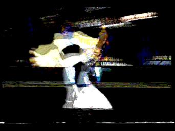
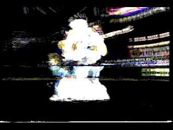
(a) RGB frame

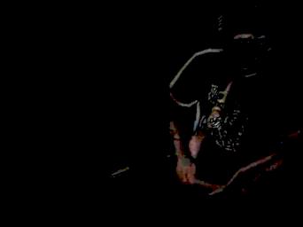
(b) $\zeta$=2

(c) $\zeta$=3

(d) $\zeta$=5

(e) $\zeta$=10

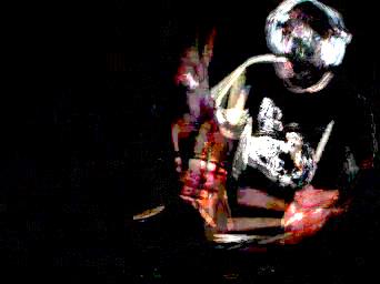
(f) $\zeta$=15

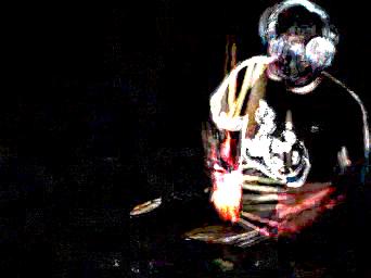
(g) $\zeta$=30

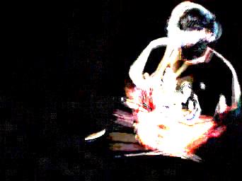
(h) $\zeta$=60

Figure 9: Comparison of 3-channel SMAID images with varying number of frames summarized per channel ($\zeta$) for two sequences from UCF101 dataset. As is clear, higher $\zeta$ leads to cluttered image, while smaller $\zeta$ fails to capture sufficient motion. Also, note that for each SMAID image, the temporal order is mapped to colors Red $<$ Green $<$ Blue.

9.6 Comparisons to the State of the Art

In Tables 8, 9, and 10, we present comparisons of our full framework (RGB + FLOW + SMAID) against state-of-the-art approaches on the four datasets, averaging the performance on all splits. On the MPII cooking activities dataset, our kernelized correlation pooling scheme shows an overall mAP of 68% (Table 2). This is better than the results in recent CNN based approaches such as Chéron et al. (2015) (62.3%) and better than non-CNN based, yet state of the art schemes such as Lan et al. (2015) (66.8%). Further, we see that incorporating trajectory features into our framework substantially improves our accuracy further to 74.7% (Table 8) outperforming all other approaches. On the JHMDB dataset, our correlation pooling scheme provides an average accuracy of 62%, while the kernelization scheme improves this to 72.7%. In comparison to the CNN based results in Chéron et al. (2015), our results are about 10% better. Further, incorporating BKCP and trajectory features increases our performance to 77.3%, which is better than the next best method by about 5.1%. These comparisons clearly demonstrate the effectiveness of our methodology against prior works. On HMDB dataset, our combination of KCP, BKCP, with dense trajectory features demonstrate state of the art performance, better by about 1.3%, on a similar capacity VGG-16 model Feichtenhofer et al. (2016b), and providing about 2.2% improvement over the respective ResNet model (70.3% to 72.5%) when combined with Fisher vector encoded trajectory features. Similar results are seen on UCF101 dataset, with our scheme outperforming a recent state of the art Feichtenhofer et al. (2017) by 0.5%. We also provide comparison to the recent I3D model Carreira and Zisserman (2017), however note that this model was pre-trained using the larger Kinetics-400 dataset Zisserman et al. (2017), and thus the results are not strictly comparable to those on other methods or ours (that do not use external dataset). From the tables, it is clear that our scheme is independent of the CNN architecture and is consistent in the improvements that it produces in comparison to first-order pooling schemes (Table 1 and Table 2).

9.7 Analysis of Results

In this section, we provide more analysis of our results, summarizing when second-order methods improved the performance in the datasets that we use. In Figure 7 and Table 7, we provide the accuracy of each class when using KCP as against those from state of the art methods on the JHMDB and the MPII Cooking activities datasets respectively. On the MPII dataset, we outperform Zhou et al. (2015) on 28 sequences (out of 64), and in most cases the improvement is substantial. On the JHMDB dataset, we outperform the method in Chéron et al. (2015) on 12 sequences against the 21 actions in the dataset. As seen from Table 7, actions such as Dry, Cut apart, Cut slices, etc. that involve subtle motion cues, benefit most from using KCP. In Table 11, we compare MPII cooking activities classes that are most corrected by SMAID images. We see that actions such as Change temperature and spice, that involve subtle motions, benefit significantly from SMAID images. Qualitative SMAID images from the MPII cooking activities and the JHMDB dataset are provided in Figure 8 and Figure 9 using a three-channel SMAID, each channel using 7 frames.

9.8 Experiments on the Kinetics-600 Dataset

The experiments we presented above use relatively smaller datasets, while there are much larger action recognition datasets available now Monfort et al. (2018); Zisserman et al. (2017); Gu et al. (2017). To explore the benefits of our proposed approach to such large scale datasets, we now present experiments on the recently introduced Kinetics-600 Zisserman et al. (2017) dataset, which is one of the largest action recognition datasets. This dataset consists of about 460K trimmed video sequences, each video 10 seconds long and annotated for one of 600 pre-defined categories. The dataset is split into 430K training and 30K validation sequences. However, as the dataset only provides Youtube web-links and not videos themselves, not all videos could be downloaded. At the time we ran our experiments only about 390K videos for training and 26,615 videos for validation were available. The rest of the sequences were unavailable despite several downloading attempts. We present results using the available clips.

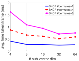
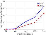
Figure 10: Computational performance analysis of BKCP, TCP, and KCP. Left: Time taken against increasing number of permutations and sub-vector dimensionality in BKCP with a feature dimensionality of 4096. Right: Time taken for TCP and BKCP for increasing number of action classes. Plots show average timing in milli-seconds.

For feature extraction, we used the state-of-the-art I3D action recognition model Carreira and Zisserman (2017), which is pre-trained on the earlier Kinetics-400 dataset. As the intention of our experiments is to show the benefits of our pooling scheme on large scale datasets, we did not fine-tune this model on Kinetics-600, instead we passed the RGB sequences through the pre-trained I3D model (using the Inception-V3 architecture), and extracted features from the last pooling layer (Max5c). These features are of size $2\times 7\times 7\times 1024$, which are average-pooled across the spatial $7\times 7$ dimensions, and reshaped to 2048-D vectors. We used a sliding window over the clips to generate a sequence of such features with a window size of 16 and a temporal stride of 8 frames.

As we cannot apply our KCP descriptor in the proposed setting (as we do not have a network generating the class confusions), we use the BKCP variant. We explore BKCP with a sub-vector dimensionality of 4 and 8, and the number of permutations as one or four. The BKCP descriptors are used to train a multi-layer perceptron (MLP) with a single hidden layer of 4096 dimensions. We used the Adam optimizer for training the model with a learning rate of $10^{-4}$ and a batch size of 512. The model was implemented in TensorFlow and the network was trained for about 30K iterations.

The results of this experiment are provided in Table 12. We compare our BKCP against average pooling (specifically, average pooling all the I3D 2048-D descriptors from a clip, which is technically equivalent to using the original I3D model), followed by training the MLP on these averaged features. The results show that BKCP is much better than using average pooling on the I3D features, and also show that using model averaging over multiple permutations is advantageous, with our best result improving over average pooling by nearly 9%. We also explored higher values of the sub-vector size and the number of permutations, however the performance was found inferior to the results we report in Table 12, a trend consistent with Figure 6(c).

Method	#perm	p	feat dim.	Accuracy (%)
I3D Carreira and Zisserman (2017)	1	1	2048	45.9
BKCP	1	4	3072	49.02
BKCP	4	4	3072	50.9
BKCP	1	8	7168	49.1
BKCP	4	8	7168	54.7
BKCP	8	8	7168	49.8

Table 12: Comparisons on the Kinetics-600 dataset using only the RGB stream. $p$ denotes the sub-vector dimensionality.

RP Fernando et al. (2015b)	GRP Cherian et al. (2017a)	BKRP Cherian et al. (2018)	KRPFSCherian et al. (2018)	BKCP	KCP
1.1	3.8	6.7	9.5	0.43	0.005

Table 13: Avg. run time (time taken / frame) – in milli-seconds using features of 2048D. BKCP used a sub-vector size of 8 and 4 permutations. KCP uses 51 action classes (as in HMDB dataset).

9.9 Run Time Analysis

In this section, we analyze the computational performance of our schemes for various parameter choices. We present two plots in Figures 10 and 10; the former analyzing the time taken by BKCP for various choices of the sub-vector dimension (using a fixed feature dimensionality of 4096) and the number of permutations used in the model averaging, while the latter plotting the performance of TCP and KCP against increasing number of action classes. All the timing experiments used a single core Intel Xeon 2.1GHz CPU and using a Matlab implementation of the algorithms. The timings (in ms) are obtained by averaging over 50 runs. As is clear from the plots, the more the number of permutations used in BKCP, the time taken increases, however is still around 1ms per frame. Further, appropriate choices of the sub-vector dimensionality could improve the effective computational complexity (as we saw in Section 4. As for the plots in Figure 10, it is clear that the time taken increases with the number of action classes, and TCP is slightly cheaper than KCP.

In Table. 13, we compare the run time of our descriptors against some recently introduced pooling schemes, such as rank pooling Fernando et al. (2015b), generalized rank pooling Cherian et al. (2017a), and the kernelized rank pooling Cherian et al. (2018). All these pooling schemes need to solve an optimization scheme for generating the final descriptor. As is clear, our second-order pooling schemes show significantly better run time performance against these recent schemes, and KCP was found to be 100x faster than for example rank pooling, under the same experimental settings. For all the schemes, we used the Matlab implementations and was run under exactly the same settings.

10 Conclusions

In this paper, we proposed a temporal pooling scheme, temporal correlation pooling, based on the correlations between temporal evolution of classifier scores. Our scheme produces positive definite matrices as descriptors, allowing the use rich mathematical (Riemannian) geometries for non-linear feature pooling. While, our basic descriptor scales quadratically against the number of action classes, we proposed a simple approximation to it that scales linearly. We also proposed a novel sub-sequence representation, SMAID, that can dramatically increase the temporal receptive fields of CNNs, thereby improving action classification performance. Using SMAID and temporal correlation pooling schemes, we proposed a novel three-stream end-to-end learnable CNN architecture for action classification. The utility of each of our contributions was substantiated via experiments on four challenging action recognition benchmarks, and the scalability and relevance of the scheme further substantiated via experiments on the Kinetics-600 action recognition dataset.

Acknowledgements: This research was supported by the Australian Research Council (ARC) through the Centre of Excellence for Robotic Vision (CE140100016) and was undertaken with the resources from the National Computational Infrastructure (NCI) at the Australian National University. The authors also thank Dr. Edison Guo (ANU) for helpful discussions. This is a pre-print of an article published in International Journal of Computer vision. The final authenticated version is available online at:
https://doi.org/10.1007/s11263-018-1111-5

References

- Arsigny et al. [2006] Vincent Arsigny, Pierre Fillard, Xavier Pennec, and Nicholas Ayache. Log-euclidean metrics for fast and simple calculus on diffusion tensors. Magnetic resonance in medicine, 56(2):411–421, 2006.
- Baccouche et al. [2011] Moez Baccouche, Franck Mamalet, Christian Wolf, Christophe Garcia, and Atilla Baskurt. Sequential deep learning for human action recognition. In Human Behavior Understanding, pages 29–39. 2011.
- Bilen et al. [2016] Hakan Bilen, Basura Fernando, Efstratios Gavves, Andrea Vedaldi, and Stephen Gould. Dynamic image networks for action recognition. In CVPR, 2016.
- Blank et al. [2005] Moshe Blank, Lena Gorelick, Eli Shechtman, Michal Irani, and Ronen Basri. Actions as space-time shapes. In ICCV. IEEE, 2005.
- Bojanowski et al. [2014] Piotr Bojanowski, Rémi Lajugie, Francis Bach, Ivan Laptev, Jean Ponce, Cordelia Schmid, and Josef Sivic. Weakly supervised action labeling in videos under ordering constraints. In ECCV. 2014.
- Cai et al. [2014] Zhuowei Cai, Limin Wang, Xiaojiang Peng, and Yu Qiao. Multi-view super vector for action recognition. In CVPR, 2014.
- Carreira and Zisserman [2017] Joao Carreira and Andrew Zisserman. Quo vadis, action recognition? a new model and the kinetics dataset. In CVPR, pages 4724–4733. IEEE, 2017.
- Carreira et al. [2012] Joao Carreira, Rui Caseiro, Jorge Batista, and Cristian Sminchisescu. Semantic segmentation with second-order pooling. In ECCV. 2012.
- Chaquet et al. [2013] Jose M Chaquet, Enrique J Carmona, and Antonio Fernández-Caballero. A survey of video datasets for human action and activity recognition. Computer Vision and Image Understanding, 117(6):633–659, 2013.
- Chatfield et al. [2014] Ken Chatfield, Karen Simonyan, Andrea Vedaldi, and Andrew Zisserman. Return of the devil in the details: Delving deep into convolutional nets. arXiv preprint arXiv:1405.3531, 2014.
- Chen and Yuille [2014] Xianjie Chen and Alan L Yuille. Articulated pose estimation by a graphical model with image dependent pairwise relations. In NIPS, 2014.
- Cherian et al. [2013] Anoop Cherian, Suvrit Sra, Arindam Banerjee, and Nikolaos Papanikolopoulos. Jensen-bregman logdet divergence with application to efficient similarity search for covariance matrices. PAMI, 35(9):2161–2174, 2013.
- Cherian et al. [2017a] Anoop Cherian, Basura Fernando, Mehrtash Harandi, and Stephen Gould. Generalized rank pooling for action recognition. In CVPR, 2017a.
- Cherian et al. [2017b] Anoop Cherian, Piotr Koniusz, and Stephen Gould. Higher-order pooling of CNN features via kernel linerization for action recognition. In WACV, 2017b.
- Cherian et al. [2018] Anoop Cherian, Suvrit Sra, Stephen Gould, and Richard Hartley. Non-linear temporal subspace representations for activity recognition. In CVPR, pages 2197–2206, 2018.
- Chéron et al. [2015] Guilhem Chéron, Ivan Laptev, and Cordelia Schmid. P-CNN: Pose-based CNN features for action recognition. arXiv preprint arXiv:1506.03607, 2015.
- Davis and Bobick [1997] James W Davis and Aaron F Bobick. The representation and recognition of human movement using temporal templates. In CVPR. IEEE, 1997.
- Donahue et al. [2014] Jeff Donahue, Lisa Anne Hendricks, Sergio Guadarrama, Marcus Rohrbach, Subhashini Venugopalan, Kate Saenko, and Trevor Darrell. Long-term recurrent convolutional networks for visual recognition and description. arXiv preprint arXiv:1411.4389, 2014.
- Duchenne et al. [2009] Olivier Duchenne, Ivan Laptev, Josef Sivic, Francis Bach, and Jean Ponce. Automatic annotation of human actions in video. In ICCV, 2009.
- Feichtenhofer et al. [2016a] Christoph Feichtenhofer, Axel Pinz, and Richard Wildes. Spatiotemporal residual networks for video action recognition. In NIPS, 2016a.
- Feichtenhofer et al. [2016b] Christoph Feichtenhofer, Axel Pinz, and Andrew Zisserman. Convolutional two-stream network fusion for video action recognition. In CVPR, 2016b.
- Feichtenhofer et al. [2017] Christoph Feichtenhofer, Axel Pinz, and Richard P Wildes. Spatiotemporal multiplier networks for video action recognition. In CVPR. IEEE, 2017.
- Fernando et al. [2015a] Basura Fernando, Efstratios Gavves, Jose M. Oramas, Amir Ghodrati, and Tinne Tuytelaars. Modeling video evolution for action recognition. In CVPR, 2015a.
- Fernando et al. [2015b] Basura Fernando, Efstratios Gavves, Jose M Oramas, Amir Ghodrati, and Tinne Tuytelaars. Modeling video evolution for action recognition. In CVPR, 2015b.
- Gall et al. [2011] Juergen Gall, Angela Yao, Negin Razavi, Luc Van Gool, and Victor Lempitsky. Hough forests for object detection, tracking, and action recognition. PAMI, 33(11):2188–2202, 2011.
- Girdhar et al. [2017] Rohit Girdhar, Deva Ramanan, Abhinav Gupta, Josef Sivic, and Bryan Russell. Actionvlad: Learning spatio-temporal aggregation for action classification. In CVPR, volume 2, page 3, 2017.
- Gkioxari and Malik [2015] Georgia Gkioxari and Jitendra Malik. Finding action tubes. In CVPR, 2015.
- Gu et al. [2017] Chunhui Gu, Chen Sun, David A Ross, Carl Vondrick, Caroline Pantofaru, Yeqing Li, Sudheendra Vijayanarasimhan, George Toderici, Susanna Ricco, Rahul Sukthankar, et al. AVA: a video dataset of spatio-temporally localized atomic visual actions. CoRR, abs/1705.08421, 4, 2017.
- Guo et al. [2013] Kai Guo, Prakash Ishwar, and Janusz Konrad. Action recognition from video using feature covariance matrices. TIP, 2013.
- He et al. [2016] Kaiming He, Xiangyu Zhang, Shaoqing Ren, and Jian Sun. Deep residual learning for image recognition. In CVPR, 2016.
- Herath et al. [2017] Samitha Herath, Mehrtash Harandi, and Fatih Porikli. Going deeper into action recognition: A survey. Image and Vision Computing, 60:4 – 21, 2017. ISSN 0262-8856. Regularization Techniques for High-Dimensional Data Analysis.
- Hoeting et al. [1999] Jennifer A Hoeting, David Madigan, Adrian E Raftery, and Chris T Volinsky. Bayesian model averaging: a tutorial. Statistical science, pages 382–401, 1999.
- Huang and Van Gool [2017] Zhiwu Huang and Luc Van Gool. A riemannian network for spd matrix learning. In AAAI, 2017.
- Ionescu et al. [2015] Catalin Ionescu, Orestis Vantzos, and Cristian Sminchisescu. Matrix backpropagation for deep networks with structured layers. In ICCV, 2015.
- Jebara and Kondor [2003] Tony Jebara and Risi Kondor. Bhattacharyya and expected likelihood kernels. In Learning theory and kernel machines, pages 57–71. Springer, 2003.
- Jégou et al. [2009] H. Jégou, M. Douze, and C. Schmid. On the Burstiness of Visual Elements. CVPR, 2009.
- Jegou et al. [2011] Herve Jegou, Matthijs Douze, and Cordelia Schmid. Product quantization for nearest neighbor search. PAMI, 33(1):117–128, 2011.
- Jhuang et al. [2013] Hueihan Jhuang, Juergen Gall, Silvia Zuffi, Cordelia Schmid, and Michael J Black. Towards understanding action recognition. In ICCV, 2013.
- Ji et al. [2013] Shuiwang Ji, Wei Xu, Ming Yang, and Kai Yu. 3d convolutional neural networks for human action recognition. PAMI, 35(1):221–231, 2013.
- Karpathy et al. [2014] Andrej Karpathy, George Toderici, Sachin Shetty, Tommy Leung, Rahul Sukthankar, and Li Fei-Fei. Large-scale video classification with convolutional neural networks. In CVPR, 2014.
- Klaser et al. [2008] Alexander Klaser, Marcin Marszałek, and Cordelia Schmid. A spatio-temporal descriptor based on 3d-gradients. In BMVC, 2008.
- Koniusz et al. [2016] Piotr Koniusz, Anoop Cherian, and Fatih Porikli. Tensor representations via kernel linearization for action recognition from 3D skeletons. In ECCV, 2016.
- Krizhevsky et al. [2012] Alex Krizhevsky, Ilya Sutskever, and Geoffrey E Hinton. Imagenet classification with deep convolutional neural networks. In NIPS, 2012.
- Kuehne et al. [2011] Hildegard Kuehne, Hueihan Jhuang, Estíbaliz Garrote, Tomaso Poggio, and Thomas Serre. Hmdb: a large video database for human motion recognition. In ICCV. IEEE, 2011.
- Lan et al. [2014] Tian Lan, Tsung-Chuan Chen, and Silvio Savarese. A hierarchical representation for future action prediction. In ECCV. 2014.
- Lan et al. [2015] Tian Lan, Yuke Zhu, Amir Roshan Zamir, and Silvio Savarese. Action recognition by hierarchical mid-level action elements. In ICCV, 2015.
- Laptev [2005] Ivan Laptev. On space-time interest points. International Journal of Computer Vision, 64(2-3):107–123, 2005.
- Le et al. [2011] Quoc V Le, Will Y Zou, Serena Y Yeung, and Andrew Y Ng. Learning hierarchical invariant spatio-temporal features for action recognition with independent subspace analysis. In CVPR, 2011.
- Lei et al. [2012] Jinna Lei, Xiaofeng Ren, and Dieter Fox. Fine-grained kitchen activity recognition using RGB-D. In ACM Conference on Ubiquitous Computing, 2012.
- Li et al. [2013] Peihua Li, Qilong Wang, Wangmeng Zuo, and Lei Zhang. Log-euclidean kernels for sparse representation and dictionary learning. In ICCV, 2013.
- Monfort et al. [2018] Mathew Monfort, Bolei Zhou, Sarah Adel Bargal, Alex Andonian, Tom Yan, Kandan Ramakrishnan, Lisa Brown, Quanfu Fan, Dan Gutfruend, Carl Vondrick, et al. Moments in time dataset: one million videos for event understanding. arXiv preprint arXiv:1801.03150, 2018.
- Newell et al. [2016] Alejandro Newell, Kaiyu Yang, and Jia Deng. Stacked hourglass networks for human pose estimation. In ECCV. Springer, 2016.
- Ni et al. [2014] Bingbing Ni, Vignesh R Paramathayalan, and Philippe Moulin. Multiple granularity analysis for fine-grained action detection. In CVPR, 2014.
- Oneata et al. [2013] Dan Oneata, Jakob Verbeek, and Cordelia Schmid. Action and event recognition with fisher vectors on a compact feature set. In ICCV, 2013.
- Pascanu et al. [2013] Razvan Pascanu, Tomas Mikolov, and Yoshua Bengio. On the difficulty of training recurrent neural networks. ICML, 2013.
- Peng et al. [2014] Xiaojiang Peng, Changqing Zou, Yu Qiao, and Qiang Peng. Action recognition with stacked fisher vectors. In ECCV. Springer, 2014.
- Peng et al. [2016] Xiaojiang Peng, Limin Wang, Xingxing Wang, and Yu Qiao. Bag of visual words and fusion methods for action recognition: Comprehensive study and good practice. CVIU, 2016.
- Pennec et al. [2006] Xavier Pennec, P. Fillard, and N. Ayache. A riemannian framework for tensor computing. International Journal of Computer Vision, 66(1):41–66, 2006.
- Pirsiavash and Ramanan [2014] Hamed Pirsiavash and Deva Ramanan. Parsing videos of actions with segmental grammars. In CVPR, 2014.
- Pishchulin et al. [2014] Leonid Pishchulin, Mykhaylo Andriluka, and Bernt Schiele. Fine-grained activity recognition with holistic and pose based features. In Pattern Recognition, pages 678–689. Springer, 2014.
- Prest et al. [2012] Alessandro Prest, Cordelia Schmid, and Vittorio Ferrari. Weakly supervised learning of interactions between humans and objects. PAMI, 34(3):601–614, 2012.
- Ren et al. [2015] Shaoqing Ren, Kaiming He, Ross Girshick, and Jian Sun. Faster R-CNN: Towards real-time object detection with region proposal networks. In NIPS, pages 91–99, 2015.
- Rohrbach et al. [2012] Marcus Rohrbach, Sikandar Amin, Mykhaylo Andriluka, and Bernt Schiele. A database for fine grained activity detection of cooking activities. In CVPR, 2012.
- Rohrbach et al. [2015] Marcus Rohrbach, Anna Rohrbach, Michaela Regneri, Sikandar Amin, Mykhaylo Andriluka, Manfred Pinkal, and Bernt Schiele. Recognizing fine-grained and composite activities using hand-centric features and script data. arXiv preprint arXiv:1502.06648, 2015.
- Ryoo and Aggarwal [2006] Michael S Ryoo and Jake K Aggarwal. Recognition of composite human activities through context-free grammar based representation. In CVPR, 2006.
- Sadanand and Corso [2012] Sreemanananth Sadanand and Jason J Corso. Action bank: A high-level representation of activity in video. In CVPR, 2012.
- Simonyan and Zisserman [2014] Karen Simonyan and Andrew Zisserman. Two-stream convolutional networks for action recognition in videos. In NIPS, 2014.
- Soomro et al. [2012] Khurram Soomro, Amir Roshan Zamir, and Mubarak Shah. UCF101: a dataset of 101 human actions classes from videos in the wild. arXiv preprint arXiv:1212.0402, 2012.
- Sra [2011] Suvrit Sra. Positive definite matrices and the symmetric stein divergence. Technical report, 2011.
- Srivastava et al. [2015] Nitish Srivastava, Elman Mansimov, and Ruslan Salakhutdinov. Unsupervised learning of video representations using LSTMs. In ICML, 2015.
- Sun and Nevatia [2014] Chen Sun and Ram Nevatia. Discover: Discovering important segments for classification of video events and recounting. In CVPR, 2014.
- Tang et al. [2012] Kevin Tang, Li Fei-Fei, and Daphne Koller. Learning latent temporal structure for complex event detection. In CVPR, 2012.
- Tompson et al. [2015] Jonathan Tompson, Ross Goroshin, Arjun Jain, Yann LeCun, and Christopher Bregler. Efficient object localization using convolutional networks. In CVPR, 2015.
- Tompson et al. [2014] Jonathan J Tompson, Arjun Jain, Yann LeCun, and Christoph Bregler. Joint training of a convolutional network and a graphical model for human pose estimation. In NIPS, 2014.
- Tran et al. [2015] Du Tran, Lubomir D Bourdev, Rob Fergus, Lorenzo Torresani, and Manohar Paluri. Learning spatiotemporal features with 3D convolutional networks. In ICCV, 2015.
- Vedaldi and Zisserman [2012] Andrea Vedaldi and Andrew Zisserman. Efficient additive kernels via explicit feature maps. PAMI, 34(3):480–492, 2012.
- Wang et al. [2013a] Chunyu Wang, Yizhou Wang, and Alan L Yuille. An approach to pose-based action recognition. In CVPR, 2013a.
- Wang and Schmid [2013] Heng Wang and Cordelia Schmid. Action recognition with improved trajectories. In ICCV, 2013.
- Wang et al. [2013b] Heng Wang, Alexander Kläser, Cordelia Schmid, and Cheng-Lin Liu. Dense trajectories and motion boundary descriptors for action recognition. IJCV, 103(1):60–79, 2013b.
- Wang et al. [2017] Jue Wang, Anoop Cherian, and Fatih Porikli. Ordered pooling of optical flow sequences for action recognition. In WACV, 2017.
- Wang et al. [2018] Jue Wang, Anoop Cherian, Fatih Porikli, and Stephen Gould. Video representation learning using discriminative pooling. In Proceedings of the IEEE Conference on Computer Vision and Pattern Recognition, pages 1149–1158, 2018.
- Wang et al. [2015] Limin Wang, Yu Qiao, and Xiaoou Tang. Action recognition with trajectory-pooled deep-convolutional descriptors. In CVPR, 2015.
- Wang et al. [2016] Limin Wang, Yuanjun Xiong, Zhe Wang, Yu Qiao, Dahua Lin, Xiaoou Tang, and Luc Van Gool. Temporal segment networks: Towards good practices for deep action recognition. In ECCV, 2016.
- Wei et al. [2016] Shih-En Wei, Varun Ramakrishna, Takeo Kanade, and Yaser Sheikh. Convolutional pose machines. In CVPR, 2016.
- Wu et al. [2015] Chenxia Wu, Jiemi Zhang, Silvio Savarese, and Ashutosh Saxena. Watch-n-patch: Unsupervised understanding of actions and relations. In CVPR, 2015.
- Yao et al. [2011a] Angela Yao, Juergen Gall, Gabriele Fanelli, and Luc J Van Gool. Does human action recognition benefit from pose estimation?. In BMVC, 2011a.
- Yao and Fei-Fei [2012] Bangpeng Yao and Li Fei-Fei. Action recognition with exemplar based 2.5 d graph matching. In ECCV. 2012.
- Yao et al. [2011b] Bangpeng Yao, Xiaoye Jiang, Aditya Khosla, Andy Lai Lin, Leonidas Guibas, and Li Fei-Fei. Human action recognition by learning bases of action attributes and parts. In ICCV, 2011b.
- Yu and Salzmann [2017] Kaicheng Yu and Mathieu Salzmann. Second-order convolutional neural networks. arXiv preprint arXiv:1703.06817, 2017.
- Yuan et al. [2009] Chunfeng Yuan, Weiming Hu, Xi Li, Stephen Maybank, and Guan Luo. Human action recognition under log-euclidean riemannian metric. In ACCV. 2009.
- Yue-Hei Ng et al. [2015] Joe Yue-Hei Ng, Matthew Hausknecht, Sudheendra Vijayanarasimhan, Oriol Vinyals, Rajat Monga, and George Toderici. Beyond short snippets: Deep networks for video classification. In CVPR, 2015.
- Zhou et al. [2014] Yang Zhou, Bingbing Ni, Shuicheng Yan, Pierre Moulin, and Qi Tian. Pipelining localized semantic features for fine-grained action recognition. In ECCV. 2014.
- Zhou et al. [2015] Yang Zhou, Bingbing Ni, Richang Hong, Meng Wang, and Qi Tian. Interaction part mining: A mid-level approach for fine-grained action recognition. In CVPR, 2015.
- Zisserman et al. [2017] Andrew Zisserman, Joao Carreira, Karen Simonyan, Will Kay, Brian Zhang, Chloe Hillier, Sudheendra Vijayanarasimhan, Fabio Viola, Tim Green, Trevor Back, et al. The kinetics human action video dataset. 2017.
- Zuffi and Black [2013] Silvia Zuffi and Michael J Black. Puppet flow. IJCV, 101(3):437–458, 2013.