Partially separable convexly-constrained optimization
with non-Lipschitzian singularities and its complexity

Abstract

An adaptive regularization algorithm using high-order models is proposed for partially separable convexly constrained nonlinear optimization problems whose objective function contains non-Lipschitzian $\ell_{q}$-norm regularization terms for $q\in(0,1)$. It is shown that the algorithm using an $p$-th order Taylor model for $p$ odd needs in general at most $O(\epsilon^{-(p+1)/p})$ evaluations of the objective function and its derivatives (at points where they are defined) to produce an $\epsilon$-approximate first-order critical point. This result is obtained either with Taylor models at the price of requiring the feasible set to be ’kernel-centered’ (which includes bound constraints and many other cases of interest), or for non-Lipschitz models, at the price of passing the difficulty to the computation of the step. Since this complexity bound is identical in order to that already known for purely Lipschitzian minimization subject to convex constraints [9], the new result shows that introducing non-Lipschitzian singularities in the objective function may not affect the worst-case evaluation complexity order. The result also shows that using the problem’s partially separable structure (if present) does not affect complexity order either. A final (worse) complexity bound is derived for the case where Taylor models are used with a general convex feasible set.

Keywords: complexity theory, nonlinear optimization, non-Lipschitz function, $\ell_{q}$-norm regularization, partially separable problems.

1 Introduction

We consider the partially separable convexly constrained nonlinear optimization problem:

$$\min_{x\in{\cal F}}f(x)=\sum_{i\in{\cal N}}f_{i}(U_{i}x)+\sum_{i\in{\cal H}}|U_{i}x|^{q}=\sum_{i\in{\cal N}}f_{i}(x_{i})+\sum_{i\in{\cal H}}f_{i}(x_{i})$$ (1.1)

where ${\cal F}$ is a non-empty closed convex set, ${\cal N}\cup{\cal H}\stackrel{{\scriptstyle\rm def}}{{=}}{\cal M}$, ${\cal N}\cap{\cal H}=\emptyset$, $f_{i}:\hbox{I\hskip-2.0ptR}^{n}\rightarrow\hbox{I\hskip-2.0ptR}$, $q\in(0,1)$, $f_{i}(x_{i})=|x_{i}|^{q}=|U_{i}x|^{q}$ for $i\in{\cal H}$ and where, for $i\in{\cal M}$, $x_{i}\stackrel{{\scriptstyle\rm def}}{{=}}U_{i}x$ with $U_{i}$ a (fixed) $n_{i}\times n$ matrix with $n_{i}\leq n$. Without loss of generality, we assume that $\|U_{i}\|=1$ for all $i\in{\cal M}$ and that the ranges of the $U_{i}^{T}$ for $i\in{\cal N}$ span $\hbox{I\hskip-2.0ptR}^{n}$ in that the intersection of the nullspaces of the $U_{i}$ is reduced to the origin. In what follows, the “element functions” $f_{i}$ ($i\in{\cal N}$) will be “well-behaved” smooth functions with Lipschitz continuous derivatives. If ${\cal H}\neq\emptyset$, we also require that

$$n_{i}=1$$ (1.2)

and (initially at least) that the feasible set is ’kernel centered’, in the sense that, if $P_{\cal X}[\cdot]$ is the orthogonal projection ont the convex set ${\cal X}$, then, for $i\in{\cal H}$,

$$P_{\ker(U_{i})}[{\cal F}]\subseteq{\cal F}\;\;\mbox{ whenever }\;\;\ker(U_{i})\cap{\cal F}\neq\emptyset$$ (1.3)

in addition of ${\cal F}$ being convex, closed and non-empty. As will be discussed below (after Lemma 4.2), we may assume without loss of generality that, $\ker(U_{i})\cap{\cal F}\neq\emptyset$ (and thus $P_{\ker(U_{i})}[{\cal F}]\subseteq{\cal F}$) for all $i\in{\cal H}$. ’Kernel centered’ feasible sets include boxes (corresponding to bound constrained problems), spheres/cylinders centered at the origin and other sets such as

$$\left\{(x_{1},x_{2})\in\hbox{I\hskip-2.0ptR}^{n_{1}+1}\mid x_{1}\in{\cal F}_{1}\;\;\mbox{and}\;\;g_{1}(x_{1})\leq x_{2}\leq-g_{2}(x_{1})\right\},\;\;\;\;{\cal H}=\{2\},$$ (1.4)

where ${\cal F}_{1}$ is a non-empty closed convex set in $\hbox{I\hskip-2.0ptR}^{n_{1}}$ and $g_{i}(\cdot)$ are convex functions from $\hbox{I\hskip-2.0ptR}^{n_{1}}$ to IR ($i=1,2$, $n_{1}+1\leq n$) such that $g_{i}(x_{1})\leq 0$ ($i=1,2$) for $x_{1}\in{\cal F}_{1}$. Compositions using (1.4) recursively, rotations, cartesian products or intersections of such sets are also kernel-centered.

Problem (1.1) has many applications in engineering and science. Using the non-Lipschitz regularization function in the second term of the objective function $f$ has remarkable advantages for the restoration of piecewise constant images and sparse signals [4, 1, 28], and sparse variable selection, for instance in bioinformatics [14, 27]. Theory and algorithms for solving $q$-norm regularized optimization problems have been developed in [12, 15, 29].

The partially separable structure defined in problem (1.1) is ubiquitous in applications of optimization. It is most useful in the frequent case where $n_{i}\ll n$ and subsumes that of sparse optimization (in the special case where the rows of each $U_{i}$ are selected rows of the identity matrix). Moreover the decomposition in (1.1) has the advantage of being invariant for linear changes of variables (only the $U_{i}$ matrices vary).

Partially separable optimization was proposed by Griewank and Toint in [26], studied for more than thirty years (see [21, 10, 20, 11, 30] for instance) and extensively used in the popular CUTE(st) testing environment [23] as well as in the AMPL [19], LANCELOT [17] and FILTRANE [24] packages, amongst others. In particular, the design of trust-region algorithms exploiting the partially separable decomposition (1.1) was investigated by Conn, Gould, Sartenaer and Toint in [16, 18] and Shahabuddin [33].

Focussing now on the nice multivariate element functions ($i\in{\cal N}$), we note that using the partially separable nature of a function $f$ can be very useful if one wishes to use derivatives of

$$f_{\cal N}(x)\stackrel{{\scriptstyle\rm def}}{{=}}\sum_{i\in{\cal N}}f_{i}(U_{i}x)=\sum_{i\in{\cal N}}f_{i}(x_{i})$$ (1.5)

of order larger than one in the context of the $p$-th order Taylor series

$$T_{f_{{\cal N},p}}(x,s)=f_{\cal N}(x)+\sum_{j=1}^{p}\frac{1}{j!}\nabla_{x}^{j}f_{\cal N}(x)[s]^{j}.$$ (1.6)

Indeed, it may be verified that

$$\nabla_{x}^{j}f_{\cal N}(x)[s]^{j}=\sum_{i\in{\cal N}}\nabla_{x_{i}}^{j}f_{i}(x_{i})[U_{i}s]^{j}.$$ (1.7)

This last expression indicates that only the $|{\cal N}|$ tensors $\{\nabla_{x_{i}}^{j}f_{i}(x_{i})\}_{i\in{\cal N}}$ of dimension $n_{i}^{j}$ needs to be computed and stored, a very substantial gain compared to the $n^{j}$-dimensional $\nabla_{x}^{j}f_{\cal N}(x)$ when (as is common) $n_{i}\ll n$ for all $i$. It may therefore be argued that exploiting derivative tensors of order larger than 2 — and thus using the high-order Taylor series (1.6) as a local model of $f(x+s)$ in the neighbourhood of $x$ — may be practically feasible if $f$ is partially separable. Of course the same comment applies to

$$f_{\cal H}(x)\stackrel{{\scriptstyle\rm def}}{{=}}\sum_{i\in{\cal H}}f_{i}(U_{i}x)=\sum_{i\in{\cal H}}f_{i}(x_{i})$$ (1.8)

whenever the required derivatives of $f_{i}(x_{i})=|x_{i}|^{p}$ ($i\in{\cal H}$) exist.

Interestingly, the use of high-order Taylor models for optimization was recently investigated by Birgin et al. [3] in the context of adaptive regularization algorithms for unconstrained problems. Their proposal belongs to this emerging class of methods pioneered by Griewank [25], Nesterov and Polyak [32] and Cartis, Gould and Toint [6, 7] for the unconstrained case and by these last authors in [8] for the convexly constrained case of interest here. Such methods are distinguished by their excellent evaluation complexity, in that they need at most $O(\epsilon^{-(p+1)/p})$ evaluations of the objective function and their derivatives to produce an $\epsilon$-approximate first-order critical point, compared to the $O(\epsilon^{-2})$ evaluations which might be necessary for the steepest descent and Newton’s methods (see [31] and [5] for details). However, most adaptive regularization methods rely on a non-separable regularization term in the model of the objective function, making exploitation of structure difficult.

The purpose of the present paper is twofold. Its first aim is to show that worst-case evaluation complexity for nonconvex minimization subject to convex constraints is not affected by the introduction of non-Lipschitzian singularities in the objective function. The second and concurrent one is to show that this complexity is not affected either by the use of partially separable structure, if present in the problem.

The remaining of the paper is organized as follows. Section 2 establishes a necessary first-order optimality condition for the non-Lipschitzian case. Section 3 then introduces the partially separable adaptive regularization algorithm for this problem while Section 4 is devoted to its worst-case evaluation complexity analysis for the case where Taylor models are used with a kernel-centered feasible set. Section 5 drops the kernel-centered assumption for non-Lipschitz models and Taylor models. The results are discussed in Section 6 and some final conclusions and perspectives are presented in Section 7.

Notations. In what follow, $\|x\|$ denotes the Euclidean norm of the vector $x$ and $\|T\|_{p}$ the recursively induced Euclidean norm on the $p$-th order tensor $T$ (see [3, 9] for details). The notation $T[s]^{i}$ means that the tensor $T$ is applied to $i$ copies of the vector $s$. For any set ${\cal X}$, $|{\cal X}|$ denotes its cardinality. For any ${\cal I}\subseteq{\cal M}$, we also denote $f_{\cal I}(x)=\sum_{i\in{\cal I}}f_{i}(x)$.

2 First-order necessary conditions

In this section, we first present exact and approximate first-order necessary conditions for a local minimizer of problem (1.1). Such conditions for optimization problems with non-Lipschitzian singularities have been independently defined in the scaled form [15] or in subspaces [2, 14]. In a recent paper [13], KKT necessary optimality conditions for constrained optimization problems with non-Lipschitzan singularities are studied under the relaxed constant positive linear dependence and basic qualification. The above optimality conditions take the singularity into account by no longer requiring that the gradient (for unconstrained problems, say) nearly vanishes at an approximate solution $x_{\epsilon}$ (which would be impossible if the singularity is active) but by requiring that a scaled version of this requirement holds in that $\|X_{\epsilon}\nabla_{x}^{1}f(x_{\epsilon})\|$ is suitably small, where $X_{\epsilon}$ is a diagonal matrix whose diagonal entries are the components of $x_{\epsilon}$. Unfortunately, if the $i$-th component of $x_{\epsilon}$ is small but not quite small enough to consider that the singularity is active for variable $i$ (say it is equal to $2\epsilon$), the $i$-th component of $\nabla_{x}^{1}f(x)$ can be as large as a multiple of $\epsilon^{-1}$. As a result, comparing worst-case evaluation complexity bounds with those known for purely Lipschitz continuous problems (such as those proposed in [3] or [9]) may be misleading, since these latter conditions would never accept an approximate first-order critical point with such a large gradient. In order to avoid these pitfalls, we now propose a stronger definition of approximate first-order critical point for non-Lipschitzian problems where such “border-line” situations do not occur. The new definition is also makes use of subspaces but exactly reduces to the standard condition for Lipschitzian problems if the singularity is not active at $x_{\epsilon}$, even if it is close to it.

Given a vector $x\in\hbox{I\hskip-2.0ptR}^{n}$ and $\epsilon\geq 0$, denote

$${\cal C}(x,\epsilon)\stackrel{{\scriptstyle\rm def}}{{=}}\{i\in{\cal H}\ |\ |U_{i}x|\leq\epsilon\},\quad{\cal R}(x,\epsilon)\stackrel{{\scriptstyle\rm def}}{{=}}\bigcap_{i\in{\cal C}(x,\epsilon)}\ker(U_{i})=\left[\operatorname*{span}_{i\in{\cal C}{(x,\epsilon)}}\{U_{i}^{T}\}\right]^{\bot}$$

and

$${\cal W}(x,\epsilon)\stackrel{{\scriptstyle\rm def}}{{=}}{\cal N}\cup({\cal H}\setminus{\cal C}(x,\epsilon)).$$

For convenience, if $\epsilon=0$, we denote ${\cal C}(x)\stackrel{{\scriptstyle\rm def}}{{=}}{\cal C}(x,0)$, ${\cal R}(x)\stackrel{{\scriptstyle\rm def}}{{=}}{\cal R}(x,\epsilon)$ and ${\cal W}(x)\stackrel{{\scriptstyle\rm def}}{{=}}{\cal W}(x,0)$.

Observe that the definition of ${\cal R}(x,\epsilon)$ above gives that

$${\cal R}(x,\epsilon)^{\perp}\subseteq\operatorname*{span}_{i\in{\cal H}}\{U_{i}^{T}\}.$$ (2.1)

Also note that any $x\in\hbox{I\hskip-2.0ptR}^{n}$ can be decomposed uniquely as $x=y+z$ where $y\in{\cal R}(x)^{\bot}$ and $z\in{\cal R}(x)$. By the definition of ${\cal R}(x)$, it is not difficult to verify that

$$U_{i}z=0,~{}\forall i\in{\cal C}(x)\quad\mbox{and}\quad x\in{\cal R}(x).$$

Finaly note that, although $f(x)$ is nonsmooth if ${\cal H}\neq\emptyset$, $f_{{\cal W}(x,\epsilon)}(x)$ is as differentiable as the $f_{i}(x)$ for $i\in{\cal N}$ and any $\epsilon\geq 0$. This allows us to formulate our first-order necessary condition.

Theorem 2.1

If $x_{*}\in{\cal F}$ is a local minimizer of problem (1.1), then $$\chi_{f}(x_{*})=0,$$ (2.2) where, for any $x\in{\cal F}$, $$\chi_{f}(x_{*})=\chi_{f}(x_{*},0)\stackrel{{\scriptstyle\rm def}}{{=}}\left|\min_{{}_{\stackrel{{\scriptstyle\scriptstyle x+d\in{\cal F}}}{{\scriptstyle d\in{\cal R}(x),\|d\|\leq 1}}}}\nabla_{x}^{1}f_{{\cal W}(x)}(x)^{T}d\right|.$$ (2.3)

• Proof.    Suppose first that ${\cal R}(x_{*})=\{0\}$ (which happens if $x_{*}=0\in{\cal F}$ and $\operatorname*{span}_{i\in{\cal H}}\{U_{i}^{T}\}=\hbox{I\hskip-2.0ptR}^{n}$). Then (2.2)-(2.3) holds vacuously. Now suppose that ${\cal R}(x_{*})$ contains at least one nonzero element. By assumption, there exists $\delta_{x_{*}}>0$ such that

  $$\begin{split}f(x_{*})&=\min\{f_{{\cal N}}(x)+f_{{\cal H}}(x)\ |\ x\in{\cal F},~{}\|x-x_{*}\|\leq\delta_{x_{*}}\}\\ &=\min\{f_{{\cal N}}(y+z)+f_{{\cal H}}(y+z)\ |\ y+z\in{\cal F},y\in{\cal R}(x_{*})^{\bot},z\in{\cal R}(x_{*}),\|y+z-x_{*}\|\leq\delta_{x_{*}}\}\\ &\leq\min\{f_{{\cal N}}(y+z)+\sum_{i\in{\cal H}}|U_{i}(y+z)|^{q}\ |\ y+z\in{\cal F},y=0,z\in{\cal R}(x_{*}),\|z-x_{*}\|\leq\delta_{x_{*}}\}\\ &=\min\{f_{{\cal N}}(z)+\sum_{i\in{\cal H}}|U_{i}z|^{q}\ |\ z\in{\cal F}\cap{\cal R}(x_{*}),\|z-x_{*}\|\leq\delta_{x_{*}}\}\\ &=\min\{f_{{\cal N}}(z)+\sum_{i\in{\cal H}\backslash{\cal C}({x_{*}})}|U_{i}z|^{q}\ |\ z\in{\cal F}\cap{\cal R}(x_{*}),\|z-x_{*}\|\leq\delta_{x_{*}}\}.\end{split}$$

  We now introduce a new problem, which is problem (1.1) reduced to ${\cal R}(x_{*})$, namely,

  $$\begin{split}\min&\quad f_{{\cal W}(x_{*})}(z)=f_{{\cal N}}(z)+\sum_{i\in{\cal H}\backslash{\cal C}(x_{*})}|U_{i}z|^{q},\\ \mbox{s.t.}&\quad z\in{\cal F}\cap{\cal R}(x_{*})\end{split}$$ (2.4)

  where the gradient $\nabla_{z}^{1}f_{{\cal W}(x_{*})}(z)$ is locally Lipschitz continuous in some (bounded) neighborhood of $x_{*}$. It then follows from $x_{*}\in{\cal R}(x_{*})$ that

  $$f_{{\cal W}(x_{*})}(x_{*})=f_{{\cal N}}(x_{*})+\sum_{i\in{\cal H}\backslash{\cal C}(x_{*})}|U_{i}x_{*}|^{q}=f(x_{*}).$$

  Therefore, we have that

  $$f_{{\cal W}(x_{*})}(x_{*})\leq\min\{f_{{\cal W}(x_{*})}(z)\ |\ z\in{\cal F}\cap{\cal C}(x_{*}),\|z-x_{*}\|\leq\delta_{x_{*}}\}$$

  which implies that $x_{*}$ is a local minimizer of problem (2.4). Hence, we have

  $$\nabla_{z}^{1}f_{{\cal W}(x_{*})}(x_{*})^{T}(z-x_{*})\geq 0,\quad z\in{\cal F}\cap{\cal R}(x_{*}).$$ (2.5)

  In addition,

  $$\{d=0\}\subseteq\{d\ \mid\ x_{*}+d\in{\cal F},d\in{\cal R}(x_{*}),\|d\|\leq 1\}\subseteq\{d\ \mid\ x_{*}+d\in{\cal F},d\in{\cal R}(x_{*})\}$$

  which gives the desired result (2.2)-(2.3). $\Box$

We call $x_{*}$ a first-order stationary point of (1.1), if $x_{*}$ satisfies the relation (2.2) in Theorem 2.1. For $\epsilon>0$, we call $x_{\epsilon}$ an $\epsilon$-approximate first-order stationary point of (1.1), if $x_{\epsilon}$ satisfies

$$\chi_{f}(x_{\epsilon},\epsilon)\stackrel{{\scriptstyle\rm def}}{{=}}\left|\min_{{}_{\stackrel{{\scriptstyle\scriptstyle x+d\in{\cal F}}}{{\scriptstyle d\in{\cal R}(x_{\epsilon},\epsilon),\|d\|\leq 1}}}}\nabla_{x}^{1}f_{{\cal W}(x_{\epsilon},\epsilon)}(x_{\epsilon})^{T}d\right|\leq\epsilon.$$ (2.6)

Theorem 2.2

Let $x_{\epsilon}$ be an $\epsilon$-approximate first-order stationary point of (1.1). Then any cluster point of $\{x_{\epsilon}\}_{\epsilon>0}$ is a first-order stationary point of problem (1.1) as $\epsilon\rightarrow 0$.

• Proof.    Suppose that $x_{*}$ is any cluster point of $\{x_{\epsilon}\}_{\epsilon>0}$. Hence there must exist an infinite sequence $\{\epsilon_{k}\}$ converging to zero and an infinite sequence $\{x_{\epsilon_{k}}\}_{k\geq 0}\subseteq\{x_{\epsilon}\}_{\epsilon>0}$ such that $x_{*}=\lim_{k\rightarrow\infty}x_{\epsilon_{k}}$ and $x_{\epsilon_{k}}$ is an $\epsilon_{k}$-approximate first-order stationary point of (1.1) for eack $k\geq 0$. If ${\cal R}(x_{*})=\{0\}$, (2.2) holds vacuously and hence $x_{*}$ is a first-order stationary point. Suppose therefore that ${\cal R}(x_{*})$ contains at least one nonzero element, implying that the dimension of ${\cal R}(x_{*})$ is strictly positive.

  First of all, we claim that there must exist $k_{*}\geq 0$ such that ${\cal R}(x_{\epsilon_{k}},\epsilon_{k})^{\bot}\subseteq{\cal R}(x_{*})^{\bot}$ for any $k\geq k_{*}$. Indeed, if that is not the case, there exists a subsequence of $\{x_{\epsilon_{k}}\}$, say $\{x_{\epsilon_{k_{j}}}\}$, such that $\lim_{j\rightarrow\infty}\epsilon_{k_{j}}=0$ and ${\cal R}(x_{\epsilon_{k_{j}}},\epsilon_{k_{j}})^{\bot}\not\subseteq{\cal R}(x_{*})^{\bot}$ for all $j$. Using now (2.1) and the fact that ${\cal H}$ is a finite set, we obtain that there must exist an $i_{0}\in{\cal H}$ such that $i_{0}\in{\cal C}(x_{\epsilon_{k_{j_{t}}}},\epsilon_{k_{j_{t}}})$ but $i_{0}\notin{\cal C}(x_{*})$ where $\{k_{j_{t}}\}\subseteq\{k_{j}\}$ with $t=1,2,\cdots$. For convenience, we continue to use $\{k_{j}\}$ to denote its subsequence $\{k_{j_{t}}\}$. Hence, we have that

  $$|U_{i_{0}}x_{\epsilon_{k_{j}}}|\leq\epsilon_{k_{j}}.$$

  Let $j$ go to infinity. It then follows from the above inequality that $|U_{i_{0}}x_{*}|=0$, which contradicts the fact that $i_{0}\notin{\cal C}(x_{*})$. Thus, we conclude that, for some $k_{*}\geq 0$ and all $k\geq k_{*}$, ${\cal R}(x_{\epsilon_{k}},\epsilon_{k})^{\bot}\subseteq{\cal R}(x_{*})^{\bot}$. Therefore we have that ${\cal R}(x_{*})\subseteq{\cal R}(x_{\epsilon_{k}},\epsilon_{k})$ for $k\geq k_{*}$.

  For any fixed $\epsilon_{k}$ approximate first-order stationary point $x_{\epsilon_{k}}$, consider the following two minimization problems.

  $$\begin{split}\min&\quad\nabla_{x}^{1}f_{{\cal W}(x_{\epsilon_{k}},\epsilon_{k})}(x_{\epsilon_{k}})^{T}d,\\ \mbox{s.t.}&\quad x_{\epsilon_{k}}+d\in{\cal F},d\in{\cal R}(x_{\epsilon_{k}},\epsilon_{k}),\|d\|\leq 1,\end{split}$$ (2.7)

  and

  $$\begin{split}\min&\quad\nabla_{x}^{1}f_{{\cal W}(x_{\epsilon_{k}},\epsilon_{k})}(x_{\epsilon_{k}})^{T}d,\\ \mbox{s.t.}&\quad x_{\epsilon_{k}}+d\in{\cal F},d\in{\cal R}(x_{*}),\|d\|\leq 1.\end{split}$$ (2.8)

  Since $d=0$ is a feasible point of both problems (2.7) and (2.8), the minimum values of (2.7) and (2.8) are both nonpositive. Moreover, it follows from ${\cal R}(x_{*})\subseteq{\cal R}(x_{\epsilon_{k}},\epsilon_{k})$ that the minimum value of (2.8) is not smaller than that of (2.7).

  Hence, from (2.6), we have that for any $x_{\epsilon_{k}}$,

  $$\left|\min_{{}_{\stackrel{{\scriptstyle\scriptstyle x_{\epsilon_{k}}+d\in{\cal F}}}{{\scriptstyle d\in{\cal R}(x_{*}),\|d\|\leq 1}}}}\nabla_{x}^{1}f_{{\cal W}(x_{\epsilon_{k}},\epsilon_{k})}(x_{\epsilon_{k}})^{T}d\right|\leq\left|\min_{{}_{\stackrel{{\scriptstyle\scriptstyle x_{\epsilon_{k}}+d\in{\cal F}}}{{\scriptstyle d\in{\cal R}(x_{\epsilon_{k}},\epsilon_{k}),\|d\|\leq 1}}}}\nabla_{x}^{1}f_{{\cal W}(x_{\epsilon_{k}},\epsilon_{k})}(x_{\epsilon_{k}})^{T}d\right|\leq\epsilon_{k}.$$ (2.9)

  Suppose that $d_{\epsilon_{k}}$ is a minimizer of problem (2.8), then (2.9) implies that

  $$-\epsilon_{k}\leq\nabla_{x}^{1}f_{{\cal W}(x_{\epsilon_{k}},\epsilon_{k})}(x_{\epsilon_{k}})^{T}d_{\epsilon_{k}}\leq 0,$$ (2.10)

  where $d_{\epsilon_{k}}$ should satisfy that $x_{\epsilon_{k}}+d_{\epsilon_{k}}\in{\cal F}$, $d_{\epsilon_{k}}\in{\cal R}(x_{*})$ and $\|d_{\epsilon_{k}}\|\leq 1$. Note that, since $d_{\epsilon_{k}}\in{\cal R}(x_{*})$,

  $$\begin{split}\nabla_{x}^{1}f_{{\cal W}(x_{\epsilon_{k}},\epsilon_{k})}(x_{\epsilon_{k}})^{T}d_{\epsilon_{k}}&=\left(\nabla_{x}f_{{\cal N}}(x_{\epsilon_{k}})+\sum_{i\in{\cal H}\setminus{\cal C}(x_{\epsilon_{k}})}q|U_{i}x_{\epsilon_{k}}|^{q-1}{\rm sign}(U_{i}x_{\epsilon_{k}})U_{i}^{T}\right)^{T}d_{\epsilon_{k}}\\ &=\nabla_{x}f_{{\cal N}}(x_{\epsilon_{k}})^{T}d_{\epsilon_{k}}+\sum_{i\in{\cal H}\setminus{\cal C}(x_{\epsilon_{k}})}q|U_{i}x_{\epsilon_{k}}|^{q-1}{\rm sign}(U_{i}x_{\epsilon_{k}})U_{i}d_{\epsilon_{k}}\\ &=\nabla_{x}f_{{\cal N}}(x_{\epsilon_{k}})^{T}d_{\epsilon_{k}}+\sum_{i\in{\cal H}}q|U_{i}x_{\epsilon_{k}}|^{q-1}{\rm sign}(U_{i}x_{\epsilon_{k}})U_{i}d_{\epsilon_{k}}.\end{split}$$ (2.11)

  From the compactness of $\{d\ |\ \|d\|\leq 1\}$, we know that there must exist a subsequence of $\{d_{\epsilon_{k}}\}$ such that $d_{\epsilon_{k_{j}}}\rightarrow d_{*}\in{\cal R}(x_{*})$ with $\|d_{*}\|\leq 1$ as $j$ goes to infinity. Since for $i\in{\cal H}\backslash{\cal C}(x_{*})$, we have $\lim_{k\rightarrow\infty}|U_{i}x_{\epsilon_{k}}|^{q-1}=|U_{i}x_{*}|^{q-1}$. Let $k$ go to infinity in (2.10) and (2.11), and we obtain that

  $$0=\nabla_{x}^{1}f_{{\cal W}(x_{\epsilon_{k}},\epsilon_{k})}(x_{*})^{T}d_{*}=\nabla f_{{\cal N}}(x_{*})^{T}d_{*}+\sum_{i\in{\cal H}\backslash{\cal C}(x_{*})}q|U_{i}x_{*}|^{q-1}{\rm sign}(U_{i}x_{*})U_{i}d_{*},$$

  which implies that

  $$\min_{{}_{\stackrel{{\scriptstyle\scriptstyle x_{*}+d\in{\cal F}}}{{\scriptstyle d\in{\cal R}(x_{*}),\|d\|\leq 1}}}}\nabla_{x}^{1}f_{{\cal W}(x_{\epsilon_{k}},\epsilon_{k})}(x_{*})^{T}d=\nabla_{x}^{1}f_{{\cal W}(x_{*})}(x_{*})^{T}d_{*}=0$$

  and completes the proof. $\Box$

3 A partially separable regularization algorithm

We now examine the desired properties of the element functions $f_{i}$ more closely. Assume first that, for $i\in{\cal N}$, each element function $f_{i}$ is $p$ times continuously differentiable and its $p$-th order derivative tensor $\nabla_{x}^{p}f_{i}$ is globally Lipschitz continuous with constant $L_{i}\geq 0$ in the sense that, for all $x_{i},y_{i}\in{\rm range}(U_{i})$,

$$\|\nabla_{x_{i}}^{p}f_{i}(x_{i})-\nabla_{x_{i}}^{p}f_{i}(y_{i})\|_{p}\leq L_{i}\|x_{i}-y_{i}\|.$$ (3.1)

It can be shown (see (4.6) below) that this assumption implies that, for $i\in{\cal N}$,

$$f_{i}(x_{i}+s_{i})=T_{f_{i},p}(x_{i},s_{i})+\frac{1}{(p+1)!}\tau_{i}L_{i}\|s_{i}\|^{p+1}\;\;\mbox{ with }\;\;|\tau_{i}|\leq 1,$$ (3.2)

where $s_{i}=U_{i}s$.

Because the quantity $\tau_{i}L_{i}$ in (3.2) is usually unknown in practice, it is impossible to use (3.2) directly to model the objective function in a neighbourhood of $x$. However, we may replace this term with an adaptive parameter $\sigma_{i}$, which yields the following $(p+1)$-th order model for the $i$-th element ($i\in{\cal N}$):

$$m_{i}(x_{i},s_{i})=T_{f_{i},p}(x_{i},s_{i})+\frac{1}{(p+1)!}\ \sigma_{i}\|s_{i}\|^{p+1}.$$ (3.3)

There is more than one possible choice for defining the element models for $i\in{\cal H}$. The first is to pursue the line of polynomial Taylor-based models, for which we need the following technical result.

Lemma 3.1

We have that, for $i\in{\cal H}$ and all $x,s\in\hbox{I\hskip-2.0ptR}^{n}$ with $U_{i}x\neq 0\neq U_{i}(x+s)$, $$|x_{i}+s_{i}|^{q}=|x_{i}|^{q}+q\sum_{j=1}^{\infty}\frac{1}{j!}\left(\prod_{\ell=1}^{j-1}(q-\ell)\right)|x_{i}|^{q-j}\mu(x_{i},s_{i})^{j},$$ (3.4) where $$\mu(x_{i},s_{i})\stackrel{{\scriptstyle\rm def}}{{=}}\left\{\begin{array}[]{ll}~{}~{}\,s_{i}&\;\;\mbox{if}\;\;x_{i}>0\;\;\mbox{and}\;\;x_{i}+s_{i}>0,\\ -s_{i}&\;\;\mbox{if}\;\;x_{i}<0\;\;\mbox{and}\;\;x_{i}+s_{i}<0,\\ -(2x_{i}+s_{i})&\;\;\mbox{if}\;\;x_{i}>0\;\;\mbox{and}\;\;x_{i}+s_{i}<0,\\ ~{}~{}\,2x_{i}+s_{i}&\;\;\mbox{if}\;\;x_{i}<0\;\;\mbox{and}\;\;x_{i}+s_{i}>0.\end{array}\right.$$ (3.5)

• Proof.    If $y\in\hbox{I\hskip-2.0ptR}_{+}$, it can be verified that the Taylor expansion $|y+z|^{q}$ at $y\neq 0$ and $y+z\in\hbox{I\hskip-2.0ptR}_{+}$ is given by

  $$[y+z]^{q}=y^{q}+q\sum_{j=1}^{\infty}\frac{1}{j!}\left[\prod_{\ell=1}^{j-1}(q-\ell)\right]y^{q-j}z^{j}.$$ (3.6)

  Let us now consider $i\in{\cal H}$. Relation (3.6) yields that, if $x_{i}>0$ and $x_{i}+s_{i}>0$,

  $$|x_{i}+s_{i}|^{q}=|x_{i}|^{q}+q\sum_{j=1}^{\infty}\frac{1}{j!}\left[\prod_{\ell=1}^{j-1}(q-\ell)\right]|x_{i}|^{q-j}s_{i}^{j}.$$ (3.7)

  By symmetry, if we have that if $x_{i}<0$ and $x_{i}+s_{i}<0$, then

  $$|x_{i}+s_{i}|^{q}=|x_{i}|^{q}+q\sum_{j=1}^{\infty}\frac{(-1)^{j}}{j!}\left[\prod_{\ell=1}^{j-1}(q-\ell)\right]|x_{i}|^{q-j}s_{i}^{j}.$$ (3.8)

  Moreover, if $x_{i}>0$ and $x_{i}+s_{i}<0$, then

  $$|x_{i}+s_{i}|^{q}=|-x_{i}|^{q}+q\sum_{j=1}^{\infty}\frac{(-1)^{j}}{j!}\left[\prod_{\ell=1}^{j-1}(q-\ell)\right]|-x_{i}|^{q-j}(2x_{i}+s_{i})^{j}.$$ (3.9)

  Symmetrically, if $x_{i}<0$ and $x_{i}+s_{i}>0$, then again,

  $$|x_{i}+s_{i}|^{q}=|-x_{i}|^{q}+q\sum_{j=1}^{\infty}\frac{1}{j!}\left[\prod_{\ell=1}^{j-1}(q-\ell)\right]|-x_{i}|^{q-j}(2x_{i}+s_{i})^{j}$$ (3.10)

  (3.4)-(3.5) then trivially results from (3.7)-(3.10) and the identity $|-x_{i}|=|x_{i}|$. $\Box$

We now slightly abuse notation by defining

$$T_{|\cdot|^{q},p}(x_{i},s_{i})\stackrel{{\scriptstyle\rm def}}{{=}}\left\{\begin{array}[]{ll}T_{x^{q},p}(x_{i},s_{i})&\;\;\mbox{if }\;\;x_{i}>0\;\;\mbox{and}\;\;x_{i}+s_{i}>0,\\[8.61108pt] T_{(-x)^{q},p}(x_{i},-s_{i})&\;\;\mbox{if }\;\;x_{i}<0\;\;\mbox{and}\;\;x_{i}+s_{i}<0,\\[8.61108pt] T_{(-x)^{q},p}(-x_{i},2x_{i}+s_{i})&\;\;\mbox{if }\;\;x_{i}>0\;\;\mbox{and}\;\;x_{i}+s_{i}<0,\\[8.61108pt] T_{x^{q},p}(-x_{i},2x_{i}+s_{i})&\;\;\mbox{if }\;\;x_{i}<0\;\;\mbox{and}\;\;x_{i}+s_{i}>0.\end{array}\right.$$ (3.11)

We are now in position to define the regularized “two-sided” model for the element function $f_{i}$ ($i\in{\cal H}$) as

$$m_{i}(x_{i},s_{i})\stackrel{{\scriptstyle\rm def}}{{=}}T_{|\cdot|^{q},p}(x_{i},s_{i}).$$ (3.12)

Figure 3.1 illustrates the two-sided model (3.11)-(3.12) for $x_{i}=-{\scriptstyle\frac{1}{2}}$, $p=3$, $q={\scriptstyle\frac{1}{2}}$.

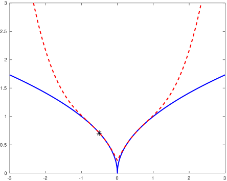
Figure 3.1: The square root function (continuous) and its two-sided model with $p=3$ evaluated at $x_{i}=-{\scriptstyle\frac{1}{2}}$ (dashed)

We may now build the complete model for $f$ at $x$ as

$$m(x,s)=\displaystyle\sum_{i\in{\cal M}}m_{i}(x_{i},s_{i}).$$ (3.13)

The algorithm considered in this paper exploits the model (3.13) as follows. At each iteration $k$, the model (3.13) taken at the iterate $x=x_{k}$ is (approximately) minimized in order to define a step $s_{k}$. If the decrease in the objective function value along $s_{k}$ is comparable to that predicted by the Taylor model, the trial point $x_{k}+s_{k}$ is accepted as the new iterate and the regularization parameters $\sigma_{i,k}$ (i.e. $\sigma_{i}$ at iteration $k$) possibly updated. The process is terminated when an approximate local minimizer is found, that is when, for some $k\geq 0$,

$$\chi_{f}(x_{k},\epsilon)\leq\epsilon.$$ (3.14)

In order to simplify notation in what follows, we make the following definitions:

$${\cal C}_{k}\stackrel{{\scriptstyle\rm def}}{{=}}{\cal C}(x_{k},\epsilon),\;\;\;\;{\cal R}_{k}\stackrel{{\scriptstyle\rm def}}{{=}}{\cal R}(x_{k},\epsilon),\;\;\;\;{\cal W}_{k}\stackrel{{\scriptstyle\rm def}}{{=}}{\cal W}(x_{k},\epsilon),$$

and

$${\cal C}_{k}^{+}\stackrel{{\scriptstyle\rm def}}{{=}}{\cal C}(x_{k}+s_{k},\epsilon),\;\;\;\;{\cal R}_{k}^{+}\stackrel{{\scriptstyle\rm def}}{{=}}{\cal R}(x_{k}+s_{k},\epsilon),\;\;\;\;{\cal W}_{k}^{+}\stackrel{{\scriptstyle\rm def}}{{=}}{\cal W}(x_{k}+s_{k},\epsilon).$$

Having defined the criticality measure (2.3), it is natural to use this measure also for terminating the approximate model minimization: to find $s_{k}$, we therefore minimize $m(x_{k},s)$ over $s$ until, for some constant $\theta\geq 0$ and some exponent $r>1$,

$$\chi_{m}(x_{k},s_{k},\epsilon)=\chi_{m_{{\cal W}_{k}^{+}}}(x_{k},s_{k},\epsilon)\leq\min\left[\,{\scriptstyle\frac{1}{4}}q^{2}\min_{i\in{\cal H}\cap{\cal W}_{k}^{+}}|U_{i}(x_{k}+s_{k})|^{r},\,\theta\|s_{k}\|^{p}\,\right]$$ (3.15)

where

$$\chi_{m_{{\cal W}_{k}^{+}}}(x_{k},s_{k},\epsilon)\stackrel{{\scriptstyle\rm def}}{{=}}\left|\min_{{}_{\stackrel{{\scriptstyle\scriptstyle x_{k}+s_{k}+d\in{\cal F}}}{{\scriptstyle d\in{\cal R}_{k}^{+},\|d\|\leq 1}}}}\nabla_{s}^{1}m_{{\cal W}_{k}^{+}}(x_{k},s_{k})^{T}d\right|.$$ (3.16)

We also require that, once $|U_{i}(x_{k}+s)|<\epsilon$ occurs for some $i\in{\cal H}$ in the course of the model minimization, it is fixed at this value, meaning that the remaining minimization is carried out in ${\cal R}(x_{k}+s,\epsilon)$. Thus the dimension of ${\cal R}(x_{k}+s,\epsilon)$ (and therefore of ${\cal R}(x_{k},\epsilon)$) is monotonically non-increasing during the step computation and across iterations. Note that computing a step $s_{k}$ satisfying (3.15) is always possible since the subspace ${\cal R}(x_{k}+s,\epsilon)$ can only become smaller during the model minimization and since we have seen in Section 2 that $\chi_{m}(x_{k},s_{k})=0$ at any local minimizer of $m_{{\cal W}(x_{k}+s,\epsilon)}(x_{k},s)$.

3.1 The algorithm

We now introduce some notation useful for describing our algorithm. Define

$$x_{i,k}\stackrel{{\scriptstyle\rm def}}{{=}}U_{i}x_{k},\;\;\;\;s_{i,k}\stackrel{{\scriptstyle\rm def}}{{=}}U_{i}s_{k}.$$

Also let

$$\delta f_{i,k}\stackrel{{\scriptstyle\rm def}}{{=}}f_{i}(x_{i,k})-f_{i}(x_{i,k}+s_{i,k})$$

$$\delta f_{k}\stackrel{{\scriptstyle\rm def}}{{=}}f_{{\cal W}_{k}^{+}}(x_{k})-f_{{\cal W}_{k}^{+}}(x_{k}+s_{k})=\sum_{i\in{\cal W}_{k}^{+}}\delta f_{i,k},$$

$$\delta m_{i,k}\stackrel{{\scriptstyle\rm def}}{{=}}m_{i}(x_{i,k},0)-m_{i}(x_{i,k},s_{i,k}),$$

$$\delta m_{k}\stackrel{{\scriptstyle\rm def}}{{=}}m_{{\cal W}_{k}^{+}}(x_{k},0)-m_{{\cal W}_{k}^{+}}(x_{k},s_{k})=\sum_{i\in{\cal W}_{k}^{+}}\delta m_{i,k},$$

and

$$\begin{array}[]{lcl}\delta T_{k}&\stackrel{{\scriptstyle\rm def}}{{=}}&T_{f_{{\cal W}_{k}^{+}},p}(x_{k},0)-T_{f_{{\cal W}_{k}^{+}},p}(x_{k},s_{k})\\[8.61108pt] &=&[T_{f_{{\cal N}},p}(x_{k},0)-T_{f_{{\cal N}},p}(x_{k},s_{k})]+[T_{|\cdot|_{{\cal H}\setminus{\cal C}_{k}^{+},p}}(x_{k},0)-T_{|\cdot|_{{\cal H}\setminus{\cal C}_{k}^{+},p}}(x_{k},s_{k})]\\[8.61108pt] &=&\delta m_{k}+\frac{\displaystyle 1}{\displaystyle(p+1)!}\displaystyle\sum_{i\in{\cal N}}\sigma_{i,k}\|s_{i,k}\|^{p+1}.\end{array}$$ (3.17)

The partially separable adaptive regularization algorithm is now formally stated as Algorithm 3.1.

Algorithm 3.1: Partially Separable Adaptive Regularization
Step 0: Initialization: $x_{0}\in{\cal F}$ and $\{\sigma_{0,i}\}_{i\in{\cal N}}>0$ are given as well as the accuracy $\epsilon\in(0,1]$ and constants $0<\gamma_{0}<1<\gamma_{1}\leq\gamma_{2}$, $\eta\in(0,1)$, $\theta\geq 0$, $\sigma_{\min}\in(0,\min_{i\in{\cal N}}\sigma_{0,i}]$ and $\kappa_{\mbox{\rm\tiny big}}>1$. Set $k=0$. Step 1: Termination: Evaluate $f(x_{k})$ and $\{\nabla_{x}^{1}f_{{\cal W}_{k}}(x_{k})\}$. If $\chi_{f}(x_{k},\epsilon)\leq\epsilon$, return $x_{\epsilon}=x_{k}$ and terminate. Otherwise evaluate $\{\nabla_{x}^{i}f_{{\cal W}_{k}}(x_{k})\}_{i=2}^{p}$. Step 2: Step computation: Compute a step $s_{k}\in{\cal R}_{k}$ such that $x_{k}+s_{k}\in{\cal F}$, $m(x_{k},s_{k})<m(x_{k},0)$ and (3.15) holds. Step 3: Step acceptance: Compute $$\rho_{k}=\frac{\displaystyle\delta f_{k}}{\displaystyle\delta T_{k}}$$ (3.18) and set $x_{k+1}=x_{k}$ if $\rho_{k}<\eta$, or $x_{k+1}=x_{k}+s_{k}$ if $\rho_{k}\geq\eta$. Step 4: Update the “nice” regularization parameters: For $i\in{\cal N}$, if $$f_{i}(x_{i,k}+s_{i,k})>m_{i}(x_{i,k},s_{i,k})$$ (3.19) set $$\sigma_{i,k+1}\in[\gamma_{1}\sigma_{i,k},\gamma_{2}\sigma_{i,k}].$$ (3.20) Otherwise, if either $$\rho_{k}\geq\eta\;\;\mbox{ and }\;\;\delta f_{i,k}\leq 0\;\;\mbox{ and }\;\;\delta f_{i,k}<\delta m_{i,k}-\kappa_{\mbox{\rm\tiny big}}|\delta f_{k}|$$ (3.21) or $$\rho_{k}\geq\eta\;\;\mbox{ and }\;\;\delta f_{i,k}>0\;\;\mbox{ and }\;\;\delta f_{i,k}>\delta m_{i,k}+\kappa_{\mbox{\rm\tiny big}}|\delta f_{k}|$$ (3.22) then set $$\sigma_{i,k+1}\in[\max[\sigma_{\min},\gamma_{0}\sigma_{i,k}],\sigma_{i,k}],$$ (3.23) else set $$\sigma_{i,k+1}=\sigma_{i,k}.$$ (3.24) Increment $k$ by one and go to Step 1.

Note that an $x_{0}\in{\cal F}$ can always be computed by projecting an infeasible starting point onto ${\cal F}$. The idea of the second and third parts of (3.21) and (3.22) is to identify cases where the model $m_{i}$ overestimates the element function $f_{i}$ to an excessive extent, leaving some space for reducing the regularization and hence allowing longer steps. The requirement that $\rho_{k}\geq\eta$ in both (3.21) and (3.22) is intended to prevent a situation where a particular regularization parameter is increased and another decreased at a given unsuccessful iteration, followed by the opposite situation at the next iteration, potentially leading to cycling. Other more elaborate mechanisms can be designed to achieve the same goal, such as attempting to reduce a given regularization parameter at most a fixed number of times before the occurence of a successful iteration, but we do not investigate those alternatives in detail here. The idea of the second and third parts of (3.21) and (3.22) is simply to identify cases where the model $m_{i}$ overestimates the element function $f_{i}$ to an excessive extent, leaving some space for reducing the regularization and hence allowing longer steps.

We note at this stage that the condition $s_{k}\in{\cal R}_{k}$ implies that

$${\cal C}_{k}\subseteq{\cal C}_{k}^{+}\;\;\mbox{ and }\;\;{\cal W}_{k}^{+}\subseteq{\cal W}_{k}.$$

Note that the above algorithm considerably simplifies in the Lipschitzian case where ${\cal H}=\emptyset$, since

$$f_{{\cal W}_{k}}(x)=f_{\cal M}(x)=f(x)$$

for all $k\geq 0$ and all $x\in{\cal F}={\cal F}_{\cal Q}$.

4 Evaluation complexity for ’kernel-centered’ fesible sets

We start our worst-case analysis by formalizing our assumptions for problem (1.1).

• AS.1    The feasible set ${\cal F}$ is closed, convex and non-empty.

• AS.2    Each element function $f_{i}$ ($i\in{\cal N}$) is $p$ times continuously differentiable in an open set containing ${\cal F}$, where $p$ is odd whenever ${\cal H}\neq\emptyset$.

• AS.3   The $p$-th derivative of each $f_{i}$ ($i\in{\cal N}$) is Lipschitz continuous on ${\cal F}$ with associated Lipschitz constant $L_{i}$ (in the sense of (3.1)).

• AS.4   There exists a constant $f_{\rm low}$ such that $f_{\cal N}(x)\geq f_{\rm low}$ for all $x\in{\cal F}$.

• AS.5   There exists a constant $\kappa^{0}_{\cal N}\geq 0$ such that

  $$\|\nabla_{x}^{j}f_{\cal N}(0)\|\leq\kappa_{\cal N}^{0}$$

  for all $j\in\{1,\ldots,p\}$.

Note that AS.4 is necessary for problem (1.1) to be well-defined. Also observe that AS.5 guarantees the existence of a constant $\kappa_{\cal N}\geq\kappa_{\cal N}^{0}$ such that

$$\|\nabla_{x}^{1}f_{\cal N}(x))\|\leq\kappa_{\cal N}\;\;\mbox{for all}\;\;x\in\{x\in{\cal F}\mid\|x\|\leq 1\}.$$ (4.1)

Obviously, AS.2 alone implies (4.1) (without the need of assuming AS.5) if ${\cal F}$ is bounded.

We first observe that our assumptions on the partially separable nature of the objective function imply the following useful bounds.

Lemma 4.1

There exist constants $0<\varsigma_{\min}\leq\varsigma_{\max}$ such that, for all $s\in\hbox{I\hskip-2.0ptR}^{m}$ and all $v\geq 1$ and for any subset ${\cal X}\subseteq{\cal M}$, $$\varsigma_{\min}^{v}\|s_{\cal X}\|^{v}\leq\sum_{i\in{\cal X}}\|s_{i}\|^{v}\leq|{\cal X}|\,\varsigma_{\max}^{v}\,\|s_{\cal X}\|^{v},$$ (4.2) where $s_{\cal X}=P_{\operatorname*{span}_{i\in{\cal X}}\{U_{i}^{T}\}}(s)$.

• Proof.    Assume that, for every $\varsigma>0$ there exists a vector $s_{\varsigma}$ in $\operatorname*{span}_{i\in{\cal X}}\{U_{i}^{T}\}$ of norm 1 such that $\max_{i\in{\cal X}}\|U_{i}s_{\varsigma}\|<\varsigma\|s_{\varsigma}\|=\varsigma$. Then taking a sequence of $\{\varsigma_{i}\}$ converging to zero and using the compactness of the unit sphere, we obtain that the sequence $\{s_{\varsigma_{i}}\}$ has at least one limit point $s_{0}$ with $\|s_{0}\|=1$ such that $\max_{i\in{\cal X}}\|U_{i}s_{0}\|=0$, which is impossible since we assumed that the intersection of the nullspaces of the $U_{i}$ is reduced to the origin. Thus our assumption is false and there is constant $\varsigma_{\min}>0$ such that, for every $s\in\operatorname*{span}_{i\in{\cal X}}\{U_{i}^{T}\}$,

  $$\max_{i\in{\cal X}}\|s_{i}\|=\max_{i\in{\cal X}}\|U_{i}s\|\geq\varsigma_{\min}\|s\|.$$

  The first inequality of (4.2) then follows from the fact that

  $$\sum_{i\in{\cal X}}\|s_{i}\|^{v}\geq\max_{i\in{\cal X}}\|s_{i}\|^{v}\geq\varsigma_{\min}^{v}\|s\|^{v}.$$

  We have also that

  $$\sum_{i\in{\cal X}}\|s_{i}\|^{v}\leq|{\cal X}|\max_{i\in{\cal X}}\|U_{i}s\|^{v}\leq|{\cal X}|\max_{i\in{\cal X}}\left(\|U_{i}\|\|s\|\right)^{v},$$

  which yields the second inequality of (4.2) with $\varsigma_{\max}=\displaystyle\max_{i\in{\cal X}}\|U_{i}\|$. $\Box$

Taken for $v=1$ and ${\cal X}={\cal N}$, this lemma states that $\sum_{i\in{\cal N}}\|\cdot\|$ is a norm on $\hbox{I\hskip-2.0ptR}^{n}$ whose equivalence constants with respect to the Euclidean one are $\varsigma_{\min}$ and $|{\cal N}|\,\varsigma_{\max}$. In most applications, these constants are very moderate numbers.

We now turn to the consequence of the Lipschitz continuity of $\nabla_{x}^{p}f_{i}$ and define, for a given $k\geq 0$ and a given constant $\phi>0$ independent of $\epsilon$,

$${\cal O}_{k,\phi}\stackrel{{\scriptstyle\rm def}}{{=}}\{i\in{\cal W}_{k}^{+}\cap{\cal H}\mid\min[\,|x_{i,k}|,\,|x_{i,k}+s_{i,k}|\,]\geq\phi\}.$$ (4.3)

Note that

$${\cal O}_{k,\phi}={\cal H}\setminus\Big{[}{\cal C}(x_{k},\phi)\cup{\cal C}(x_{k}+s_{k},\phi)\Big{]}.$$

Lemma 4.2

Suppose that AS.2 and AS.3 hold. Then, for $k\geq 0$ and $L_{\max}\stackrel{{\scriptstyle\rm def}}{{=}}\max_{i\in{\cal N}}L_{i}$, $$f_{i}(x_{i,k}+s_{i,k})=m_{i}(x_{i,k},s_{i,k})+\frac{1}{(p+1)!}\Big{[}\tau_{i,k}(p+1)L_{\max}-\sigma_{i,k}\Big{]}\|s_{i,k}\|^{p+1}\;\;\mbox{ with }\;\;|\tau_{i,k}|\leq 1,$$ (4.4) for all $i\in{\cal N}$. If, in addition, $\phi>0$ is given and independent of $\epsilon$, then there exists a constant $L(\phi)$ independent of $\epsilon$ such that $$\|\nabla_{x}^{1}f_{{\cal N}\cup{\cal O}_{k,\phi}}(x_{k}+s_{k})-\nabla_{s}^{1}m_{{\cal N}\cup{\cal O}_{k,\phi}}(x_{k},s_{k})\|\leq L(\phi)\|s_{k}\|^{p}.$$ (4.5)

• Proof.    First note that, if $f_{i}$ has a Lipschitz continuous $p$-th derivative as a function of $U_{i}x$, then (1.7) shows that it also has a Lipschitz continuous $p$-th derivative as a function of $x$. It is therefore enough to consider the element functions as functions of $x_{i}=U_{i}x$.

  AS.3 and (3.1) imply that

  $$f_{i}(x_{i,k}+s_{i,k})=T_{f_{i},p}(x_{i,k},s_{i,k})+\frac{\tau_{i,k}}{p!}L_{\max}\|s_{i,k}\|^{p+1}\;\;\mbox{ with }\;\;|\tau_{i,k}|\leq 1,$$ (4.6)

  for each $i\in{\cal N}$ (see [3] or [9, Section 2.2]), and (4.4) then follows from (3.3).

  Consider now $i\in{\cal O}_{k,\phi}$ and assume first that $x_{i,k}>\phi$ and $x_{i,k}+s_{i,k}>\phi$. Then $f_{i}(x_{i})=x_{i}^{q}$ is infinitely differentiable on the interval $[x_{i,k},x_{i,k}+s_{i,k}]\subset[\phi,\infty)$ and the norm of its $(p+1)$-st derivative tensor is bounded above on this interval by

  $$L_{\cal H}(\phi)\stackrel{{\scriptstyle\rm def}}{{=}}\left|\prod_{\ell=0}^{p+1}(q-\ell)\right|\phi^{q-p-1}.$$ (4.7)

  We then apply the same reasoning as above using the Taylor series expansion of $x_{i}^{q}$ at $x_{i,k}$ and, because of the first line of (3.11), deduce that

  $$f_{i}(x_{i,k}+s_{i,k})=m_{i}(x_{i,k},s_{i,k})+\frac{1}{(p+1)!}\tau_{i,k}(p+1)L_{\cal H}(\phi)|s_{i,k}|^{p+1}\;\;\mbox{ with }\;\;|\tau_{i,k}|\leq 1,$$ (4.8)

  and

  $$\|\nabla_{x}^{1}f_{i}(x_{i,k}+s_{i,k})-\nabla_{s}^{1}m_{i}(x_{i,k},s_{i,k})\|\leq L_{\cal H}(\phi)|s_{i,k}|^{p},$$ (4.9)

  hold in this case (see [3]). The argument is obviously similar if $x_{i,k}<-\phi$ and $x_{i,k}+s_{i,k}<-\phi$, using symmetry and the second line of (3.11). Let us now consider the case where $x_{i,k}>\phi$ and $x_{i,k}+s_{i,k}<-\phi$. The expansion (3.4) then shows that we may reason as for $x_{i,k}<-\phi$ and $x_{i,k}+s_{i,k}<-\phi$ using a Taylor expansion at $-x_{i}$ (which we know by symmetry) and the third line of (3.11). The case where $x_{i,k}<-\phi$ and $x_{i,k}+s_{i,k}>\phi$ is similar, using the fourth line of (3.11). As a consequence, (4.8) and (4.9) hold for every $i\in{\cal O}_{k,\phi}$ with Lipschitz constant $L_{\cal H}(\phi)$. Moreover, using (4.2) and the definitions (4.7),

  $$\sum_{i\in{\cal N}\cup{\cal O}_{k,\phi}}L_{i}\|s_{i}\|^{p+1}\leq\max\left[L_{\max},L_{\cal H}(\phi)\right]\sum_{i\in{\cal N}\cup{\cal O}_{k,\phi}}\|s_{i}\|^{p+1}$$

  from which (4.5) may in turn be derived from (4.9) and (4.2) with

  $$L(\phi)\stackrel{{\scriptstyle\rm def}}{{=}}|{\cal M}|\,\varsigma_{\max}^{p+1}\,\max\left[L_{\max},L_{\cal H}(\phi)\right].$$ (4.10)

  $\Box$

Note that there is no dependence on $\phi$ in $L$ if ${\cal H}=\emptyset$.

We now return to our statement that

$$\ker(U_{i})\cap{\cal F}\neq\emptyset$$ (4.11)

may be assumed without loss of generality for all $i\in{\cal H}$. Indeed, assume that (4.11) fails for $j\in{\cal H}$. Then $j\in{\cal O}_{k,\xi_{j}}$ for all $k\geq 0$, where $\xi_{j}>0$ is the distance between $\ker(U_{j})$ and ${\cal F}$, and we may transfer $j$ from ${\cal H}$ to ${\cal N}$ (possibly modifying $L_{\max}$).

The definition of the model in (3.13) also implies a simple lower bound on model decrease.

Lemma 4.3

For all $k\geq 0$, $$\delta T_{k}\geq\frac{1}{(p+1)!}\,\sigma_{\min}\sum_{i\in{\cal N}}\|s_{i,k}\|^{p+1},$$ (4.12) $s_{k}\neq 0$ and (3.18) is well-defined.

• Proof.    The bound directly follows from (3.17), the observation that the algorithm enforces $\delta m_{k}>0$ and (3.23). Moreover, $\chi_{m}(x_{k},0,\epsilon)=\chi_{f}(x_{k},\epsilon)>\epsilon$. As a consequence, (3.15) cannot hold for $s_{k}=0$ since termination would have then occured in Step 1 of Algorithm 3.1. Hence at least one $\|s_{i,k}\|$ is strictly positive because of (4.2) and (4.12) therefore implies that (3.18) is well-defined. $\Box$

We now verify that the two-sided model (3.12) is an overestimate of the function $|x|^{q}$ for all relevant $x_{i}$ and $s_{i}$.

Lemma 4.4

Suppose that AS.2 holds. Then, for $i\in{\cal H}$ and all $x_{i},s_{i}\in\hbox{I\hskip-2.0ptR}^{n}$ with $x_{i}\neq 0\neq x_{i}+s_{i}$, we have that $$|x_{i}+s_{i}|^{q}\leq m_{i}(x_{i},s_{i}).$$ (4.13)

• Proof.    Since $i\in{\cal H}$ by assumption, this implies that ${\cal H}\neq\emptyset$, and thus, by AS.2, that $p$ is odd. From the mean-value theorem, we obtain that

  $$\begin{array}[]{lcl}|x_{i}+s_{i}|^{q}&=&|x_{i}|^{q}+q\displaystyle\sum_{j=1}^{p}\frac{\displaystyle 1}{\displaystyle j!}\left[\displaystyle\prod_{\ell=1}^{j-1}(q-\ell)\right]|x_{i}|^{q-j}\mu(x_{i},s_{i})^{j}\\[8.61108pt] &&+\frac{\displaystyle 1}{\displaystyle(p+1)!}\left[\displaystyle\prod_{\ell=1}^{p}(q-\ell)\right]|U_{i}z|^{q-p-1}\mu(x_{i},s_{i})^{p+1}\end{array}$$ (4.14)

  for some $z$ such that, using symmetry, $z\in[x,x+s]$ if $(U_{i}x)(U_{i}(x+s))>0$ or $z\in[-x,x+s]$ otherwise. As a consequence, we have that

  $$|U_{i}z|\geq\min[\,|x_{i}|,\,|x_{i}+s_{i}|\,]>0.$$

  Remember now that $p$ is odd. Then, using that $q\in(0,1)$, we have that

  $$\mu(x_{i},s_{i})^{p+1}\geq 0\;\;\mbox{ and }\;\;\displaystyle\prod_{\ell=1}^{p}(q-\ell)<0.$$

  The inequality

  $$|x_{i}+s_{i}|^{q}\leq|x_{i}|^{q}+q\displaystyle\sum_{j=1}^{p}\frac{\displaystyle 1}{\displaystyle j!}\left[\displaystyle\prod_{\ell=1}^{j-1}(q-\ell)\right]|x_{i}|^{q-j}\mu(x_{i},s_{i})^{j}$$ (4.15)

  therefore immediately follows from (4.14), proving (4.13). $\Box$

We next investigate the consequences of the model’s definition (3.12) when the singularity at the origin is approached and show that the two-sided model has to remain large along the steps when $x_{i,k}$ is not too far from the singularity.

Lemma 4.5

Suppose that $p\geq 1$ is odd, $q\in(0,1)$, $i\in{\cal H}$, $|x_{i}|\in(\epsilon,1]$, and $|x_{i}+s_{i}|\geq\epsilon$. Then $$|\nabla_{s_{i}}^{1}m_{i}(x_{i},s_{i})|>{\scriptstyle\frac{1}{2}}q\,|\nabla_{s_{i}}^{1}m_{i}(x_{i},0)|.$$ (4.16)

• Proof.    Following the argument in the proof of Lemma 4.2, it is sufficient to consider that $x_{i}>0$ and $x_{i}+s_{i}>0$. From (3.11) (where $\mu(x_{i},s_{i})=s_{i}$), we have that

  $$\nabla_{s_{i}}^{1}T_{x^{q},p}(x_{i},s_{i})=q\sum_{j=1}^{p}\frac{1}{(j-1)!}\left[\prod_{\ell=1}^{j-1}(q-\ell)\right]x_{i}^{q-j}s_{i}^{j-1}.$$ (4.17)

  Define $s_{i}=\beta x_{i}$. This gives that (4.17) now reads

  $$\nabla_{s_{i}}^{1}T_{x^{q},p}(x_{i},\beta x_{i})=q\sum_{j=1}^{p}\frac{1}{(j-1)!}\left[\prod_{\ell=1}^{j-1}(q-\ell)\right]x_{i}^{q-1}\beta^{j-1},$$ (4.18)

  from which we deduce that

  $$\nabla_{s_{i}}^{1}m_{i}(x_{i},0)=\nabla_{s_{i}}^{1}T_{x^{q},p}(x_{i},0)=qx_{i}^{q-1}.$$ (4.19)

  Suppose first that $s_{i}<0$, i.e. $\beta\in(-1,0)$, and observe that $s_{i}^{j-1}<0$ exactly whenever $\displaystyle\prod_{\ell=1}^{j-1}(q-\ell)<0$, and thus, using $x_{i}\leq 1$ and (4.19), that

  $$\nabla_{s_{i}}^{1}m_{i}(x_{i},s_{i})>qx_{i}^{q-1}=\nabla_{s_{i}}^{1}m_{i}(x_{i},0)\;\;\mbox{ for }\;\;\beta\in(-1,0).$$ (4.20)

  Suppose now that $\beta\in(0,{\scriptstyle\frac{1}{3}})$. Then (4.18) implies that

  $$\begin{array}[]{lcl}\nabla_{s_{i}}^{1}T_{x^{q},p}(x_{i},\beta x_{i})&\geq&qx_{i}^{q-1}-q\displaystyle\sum_{j=2}^{p}\left|\frac{\displaystyle 1}{\displaystyle(j-1)!}\left[\displaystyle\prod_{\ell=1}^{j-1}(q-\ell)\right]\right|x_{i}^{q-1}({\scriptstyle\frac{1}{3}})^{j-1}\\[4.30554pt] &=&qx_{i}^{q-1}\left(1-\displaystyle\sum_{j=2}^{p}\left|\frac{1}{(j-1)!}\left[\displaystyle\prod_{\ell=1}^{j-1}(q-\ell)\right]\right|({\scriptstyle\frac{1}{3}})^{j-1}\right).\end{array}$$

  Observe now that

  $$\left|\frac{1}{(j-1)!}\left[\displaystyle\prod_{\ell=1}^{j-1}(q-\ell)\right]\right|=\left|\prod_{\ell=1}^{j-1}\frac{q-\ell}{\ell}\right|\leq 1,$$ (4.21)

  and therefore

  $$\begin{array}[]{lcl}\nabla_{s_{i}}^{1}T_{x^{q},p}(x_{i},\beta x_{i})&\geq&qx_{i}^{q-1}\left(1-\displaystyle\sum_{j=2}^{p}({\scriptstyle\frac{1}{3}})^{j-1}\right)\\[12.91663pt] &>&qx_{i}^{q-1}\left(1-\displaystyle\sum_{j=2}^{\infty}({\scriptstyle\frac{1}{3}})^{j-1}\right)\\[12.91663pt] &=&qx_{i}^{q-1}\left(1-\frac{{\scriptstyle\frac{1}{3}}}{1-{\scriptstyle\frac{1}{3}}}\right).\end{array}$$

  Using (4.19), this implies that

  $$\nabla_{s_{i}}^{1}T_{x^{q},p}(x_{i},\beta x_{i})\geq\frac{1}{2}\nabla_{s_{i}}^{1}T_{x^{q},p}(x_{i},0)\;\;\mbox{ for }\;\;\beta\in[0,{\scriptstyle\frac{1}{3}}].$$ (4.22)

  Suppose therefore that

  $$\beta>{\scriptstyle\frac{1}{3}}.$$ (4.23)

  We note that (4.18) gives that

  $$\nabla_{s_{i}}^{1}T_{x^{q},1}(x_{i},s_{i})=qx_{i}^{q-1}\;\;\mbox{ and }\;\;\nabla_{s_{i}}^{1}T_{x^{q},t+2}(x_{i},s_{i})=\nabla_{s_{i}}^{1}T_{x^{q},t}(x_{i},s_{i})+qx_{i}^{q-1}h_{t}(\beta)$$

  for $t\in\{1,\ldots,p-2\}$ odd, where

  $$\begin{array}[]{lcl}h_{t}(\beta)&\stackrel{{\scriptstyle\rm def}}{{=}}&\frac{\displaystyle 1}{\displaystyle t!}\left[\displaystyle\prod_{\ell=1}^{t}(q-\ell)\right]\beta^{t}+\frac{\displaystyle 1}{\displaystyle(t+1)!}\left[\displaystyle\prod_{\ell=1}^{t+1}(q-\ell)\right]\beta^{t+1}\\[12.91663pt] &=&\frac{\displaystyle 1}{\displaystyle t!}\left[\displaystyle\prod_{\ell=1}^{t}(q-\ell)\right]\beta^{t}\left(1+\frac{\displaystyle q-(t+1)}{\displaystyle t+1}\beta\right).\end{array}$$ (4.24)

  It is easy to verify that $h_{t}(\beta)$ has a root of multiplicity $t$ at zero and another root

  $$\beta_{0,t}=\frac{t+1}{t+1-q}\in\left(1\,,\,\frac{2}{2-q}\right),$$

  where the last inclusion follows from the fact that $q\in(0,1)$. We also observe that $h_{t}(\beta)$ is a polynomial of even degree (since $t$ is odd). Thus

  $$h_{t}(\beta)\geq 0\;\;\mbox{ for all }\;\;\beta\geq\frac{t+1}{t+1-q}\;\;\mbox{ and }\;\;t\in\{1,\ldots,p\}{\rm~{}odd}.$$ (4.25)

  Now

  $$\begin{array}[]{lcl}\frac{\displaystyle\nabla_{s_{i}}^{1}T_{x^{q},p}(x_{i},\beta x_{i})}{\displaystyle qx_{i}^{q-1}}&=&\frac{\displaystyle\nabla_{s_{i}}^{1}T_{x^{q},p-2}(x_{i},\beta x_{i})}{\displaystyle qx_{i}^{q-1}}+h_{p-2}(\beta)\\[6.45831pt] &=&\frac{\displaystyle\nabla_{s_{i}}^{1}T_{x^{q},1}(x_{i},\beta x_{i})}{\displaystyle qx_{i}^{q-1}}+\displaystyle\sum_{j=1,\,j{\rm~{}odd}}^{p-2}h_{j}(\beta)\\[6.45831pt] &=&1+\displaystyle\sum_{{}_{\stackrel{{\scriptstyle\scriptstyle j=1,\,j{\rm~{}odd}}}{{\scriptstyle h_{j}(\beta)<0}}}}^{p-2}h_{j}(\beta)+\displaystyle\sum_{{}_{\stackrel{{\scriptstyle\scriptstyle j=1,\,j{\rm~{}odd}}}{{\scriptstyle h_{j}(\beta)\geq 0}}}}^{p-2}h_{j}(\beta)\\[6.45831pt] &\geq&1+\displaystyle\sum_{{}_{\stackrel{{\scriptstyle\scriptstyle j=1,\,j{\rm~{}odd}}}{{\scriptstyle h_{j}(\beta)<0}}}}^{p-2}h_{j}(\beta)\end{array}$$ (4.26)

  where we used (4.18) to derive the third equality. Observe now that, because of (4.25),

  $$\begin{array}[]{lcl}\{j\in\{1,\ldots,p-2\}{\rm~{}odd}\mid h_{j}(\beta)<0\}&=&\left\{j\in\{1,\ldots,p-2\}{\rm~{}odd}\mid\beta<\frac{t+1}{t+1-q}\right\}\\[4.30554pt] &\stackrel{{\scriptstyle\rm def}}{{=}}&\{j\in\{1,\ldots,t_{0}\}|\mid j{\rm~{}odd}\}\end{array}$$ (4.27)

  for some odd integer $t_{0}\in\{1,\ldots,p-2\}$. Hence we deduce from (4.24) and (4.26) that

  $$\frac{\displaystyle\nabla_{s_{i}}^{1}T_{x^{q},p}(x_{i},\beta x_{i})}{\displaystyle qx_{i}^{q-1}}\geq 1+\sum_{j=1}^{t_{0}+1}\frac{1}{j!}\left[\prod_{\ell=1}^{j}(q-\ell)\right]\beta^{j}.$$ (4.28)

  Moreover, since $h_{t}(\beta)<0$ for $t\in\{1,\ldots,t_{0}\}$ odd and observing that the second term in the first right-hand side of (4.24) is always positive for $t$ odd, we deduce that the terms in the summation of (4.28) alternate in sign. We also note that they are decreasing in absolute value since

  $$\frac{1}{(t+1)!}\left|\prod_{\ell=1}^{t+1}(q-\ell)\right|\beta^{t+1}-\frac{1}{t!}\left|\prod_{\ell=1}^{t}(q-\ell)\right|\beta^{t}=\frac{1}{t!}\left|\prod_{\ell=1}^{t}(q-\ell)\right|\beta^{t}\left(\frac{t+1-q}{t+1}\,\beta-1\right)$$

  and (4.25) ensures that the term in brackets in the right-hand side is always negative for $q\in(0,1)$ and $t\in\{1,\ldots,t_{0}\}$ odd. Thus, keeping the first (most negative) term in (4.28), we obtain that

  $$\nabla_{s_{i}}^{1}T_{x^{q},p}(x_{i},\beta x_{i})\geq qx_{i}^{q-1}(1+(q-1)\beta)\geq\frac{q}{2-q}\nabla_{s_{i}}^{1}T_{x^{q},p}(x_{i},0)>\frac{q}{2}\nabla_{s_{i}}^{1}T_{x^{q},p}(x_{i},0).$$ (4.29)

  where we used (4.18) to deduce the second inequality. Combining (4.20), (4.22) and (4.29) then yields that (4.16) holds for all $\beta\in(-1,\infty)$, which completes the proof since $s_{i}=\beta x_{i}$. $\Box$

Our next step is to verify that the regularization parameters $\{\sigma_{i,k}\}_{i\in{\cal N}}$ cannot grow unbounded.

Lemma 4.6

Suppose that AS.2 and AS.3 hold. Then, for all $i\in{\cal N}$ and all $k\geq 0$, $$\sigma_{i,k}\in[\sigma_{\min},\sigma_{\max}],$$ (4.30) where $\sigma_{\max}\stackrel{{\scriptstyle\rm def}}{{=}}\gamma_{2}(p+1)L_{\max}$.

• Proof.    Assume that, for some $i\in{\cal N}$ and $k\geq 0$, $\sigma_{i,k}\geq(p+1)L_{i}$. Then (4.4) gives that (3.19) must fail, ensuring (4.30) because of the mechanism of the algorithm. $\Box$

We next investigate the consequences of the model’s definition (3.12) when the singularity at the origin is approached.

Lemma 4.7

Suppose that AS.2 and AS.5 (and thus (4.1)) hold and that ${\cal H}\neq\emptyset$. Let $$\omega\stackrel{{\scriptstyle\rm def}}{{=}}\min\left[1,\left(\frac{4\left[p\,\kappa_{\cal N}+\frac{|{\cal N}|}{p!}\varsigma^{p}\sigma_{\max}\right]}{q^{2}}\right)^{\frac{1}{q-1}}\right],$$ (4.31) and suppose, in addition, that $$\|s_{k}\|\leq 1$$ (4.32) and that, for some $i\in{\cal H}$, $$|x_{i,k}|\in(0,\omega).$$ (4.33) Then $$\|P_{{\cal R}{\{i\}}}[\nabla_{s}^{1}m(x_{k},s_{k})]\|\geq{\scriptstyle\frac{1}{4}}q^{2}\omega^{q-1}\;\;\mbox{ and }\;\;{\rm sgn}\left(P_{{\cal R}{\{i\}}}[\nabla_{s}^{1}m(x_{k},s_{k})]\right)={\rm sgn}(x_{i,k}+s_{i,k})$$ (4.34) where ${\cal R}_{\{i\}}\stackrel{{\scriptstyle\rm def}}{{=}}\operatorname*{span}\{U_{i}^{T}\}$.

• Proof.    Consider $i\in{\cal H}$. Suppose, for the sake of simplicity, that

  $$x_{i,k}>0\;\;\mbox{ and }\;\;x_{i,k}+s_{i,k}>0.$$ (4.35)

  We first observe that Lemma 4.5 implies that

  $$\nabla_{s_{i}}^{1}m_{i}(x_{i,k},s_{i})\geq{\scriptstyle\frac{1}{2}}q\nabla_{s_{i}}^{1}m_{i}(x_{i,k},0)\;\;\mbox{ for all }\;\;s_{i}\neq-x_{i,k}.$$ (4.36)

  Moreover,

  $$\nabla_{s}^{1}m_{\cal N}(x_{k},s_{k})=\nabla_{x}^{1}f_{\cal N}(x_{k})+\sum_{j=2}^{p}\frac{1}{(j-1)!}\nabla_{x}^{j}f_{\cal N}(x_{k})[s_{k}]^{j-1}+\frac{1}{p!}\sum_{\ell\in{\cal N}}\sigma_{\ell,k}s_{\ell,k}\|s_{\ell,k}\|^{p-1}$$

  and thus, using the contractive property of orthogonal projections,(4.32), (4.1) and (4.2), that

  $$\begin{array}[]{lcl}\|P_{{\cal R}{\{i\}}}[\nabla_{s}^{1}m_{\cal N}(x_{k},s_{k})]\|&\leq&\|\nabla_{s}^{1}m_{\cal N}(x_{k},s_{k})\|\\ &\leq&\kappa_{\cal N}[1+(p-1)]+\frac{\displaystyle|{\cal N}|}{\displaystyle p!}\varsigma^{p}\sigma_{\max}\\ &=&p\,\kappa_{\cal N}+\frac{\displaystyle|{\cal N}|}{\displaystyle p!}\varsigma^{p}\sigma_{\max}.\end{array}$$ (4.37)

  We next successively use the linearity of $P_{{\cal R}{\{i\}}}[\cdot]$, the triangle inequality, (4.36), the facts that

  $$\|U_{i}^{T}\|=1\;\;\mbox{ and }\;\;|\nabla_{s_{i}}^{1}m_{i}(x_{k},s_{k})|=q|x_{i,k}|^{q-1}\geq q\omega^{q-1},$$

  the bound (4.37), and (4.31) to deduce that

  $$\begin{array}[]{lcl}\|P_{{\cal R}{\{i\}}}[\nabla_{s}^{1}m(x_{k},s_{k})]\|&=&\|P_{{\cal R}{\{i\}}}[\nabla_{s}^{1}m_{\cal N}(x_{k},s_{k})+\nabla_{s}^{1}\displaystyle\sum_{j\in{\cal H}}m_{j}(x_{k},s_{k})]\|\\[4.30554pt] &=&\|P_{{\cal R}{\{i\}}}[\nabla_{s}^{1}m_{\cal N}(x_{k},s_{k})+\displaystyle\sum_{j\in{\cal H}}U_{j}^{T}\nabla_{s_{j}}^{1}m_{j}(x_{k},s_{k})]\|\\[4.30554pt] &=&\|P_{{\cal R}{\{i\}}}[\nabla_{s}^{1}m_{\cal N}(x_{k},s_{k})]+U_{i}^{T}\nabla_{s_{i}}^{1}m_{i}(x_{k},s_{k})\|\\[4.30554pt] &\geq&\Big{|}\|U_{i}^{T}\nabla_{s_{i}}^{1}m_{i}(x_{k},s_{k})\|-\|P_{{\cal R}{\{i\}}}[\nabla_{s}^{1}m_{\cal N}(x_{k},s_{k})]\|\Big{|}\\[4.30554pt] &\geq&{\scriptstyle\frac{1}{2}}q^{2}\omega^{q-1}-\left[p\,\kappa_{\cal N}+\frac{\displaystyle|{\cal N}|}{\displaystyle p!}\varsigma^{p}\sigma_{\max}\right]\\[4.30554pt] &\geq&{\scriptstyle\frac{1}{4}}q^{2}\omega^{q-1},\end{array}$$

  which proves the first part of (4.34) and, because of (4.36), implies the second, for the case where (4.35) holds. The proof for the cases where

  $$\Big{[}\,x_{i,k}<0\;\;\mbox{ and }\;\;x_{i,k}+s_{i,k}<0\,\Big{]}\;\;\mbox{ or }\;\;x_{i,k}(x_{i,k}+s_{i,k})<0$$

  are identical when making use of the symmetry $m_{i}(x_{i})$ with respect to the origin. $\Box$

Note that, like $\sigma_{\max}$, $\omega$ and $\beta$ only depend on problem data. In particular, they are independent of $\epsilon$. Lemma 4.7 has the following crucial consequence.

Lemma 4.8

Suppose that AS.2, AS.5 and the assumptions (4.32)–(4.33) of Lemma 4.7 hold and that ${\cal H}\neq\emptyset$. Suppose in addition that (3.15) holds at $x_{k},s_{k}$. Then, either $$|x_{i,k}+s_{i,k}|\leq\epsilon\;\;\mbox{ or }\;\;|x_{i,k}+s_{i,k}|\geq\omega\;\;\;\;(i\in{\cal H}).$$ (4.38)

• Proof.    If $j\in{\cal H}\cap{\cal C}(x_{k}+s_{k},\epsilon)$, then clearly $|x_{j,k}+s_{j,k}|\leq\epsilon$, and there is nothing more to prove. Consider therefore any $j\in{\cal H}\setminus{\cal C}_{k}^{+}\subseteq{\cal W}_{k}^{+}$ and observe that the separable nature of the linear optimization problem in (3.16) implies that

  $$\begin{array}[]{lcl}\left|\displaystyle\min_{{}_{\stackrel{{\scriptstyle\scriptstyle x_{k}+s_{k}+d\in{\cal F}}}{{\scriptstyle d\in{\cal R}_{\{j\}},\|d\|\leq 1}}}}P_{{\cal R}_{\{j\}}}[\nabla_{s}^{1}m(x_{k},s_{k})]^{T}d\right|&=&\left|\displaystyle\min_{{}_{\stackrel{{\scriptstyle\scriptstyle x_{k}+s_{k}+d\in{\cal F}}}{{\scriptstyle d\in{\cal R}_{\{j\}},\|d\|\leq 1}}}}\nabla_{s}^{1}m_{{\cal W}_{k}^{+}}(x_{k},s_{k})^{T}d\right|\\[19.37494pt] &\leq&\left|\displaystyle\min_{{}_{\stackrel{{\scriptstyle\scriptstyle x_{k}+s_{k}+d\in{\cal F}}}{{\scriptstyle d\in{\cal R}_{k}^{+},\|d\|\leq 1}}}}\nabla_{s}^{1}m_{{\cal W}_{k}^{+}}(x_{k},s_{k})^{T}d\right|\\[19.37494pt] &=&\chi_{m}(x_{k},s_{k},\epsilon)\\[4.30554pt] &\leq&{\scriptstyle\frac{1}{4}}q^{2}|x_{j,k}+s_{j,k}|^{r}.\end{array}$$ (4.39)

  Observe now that, because of the second part of (4.34) and the fact that $n_{j}=1$ because of (1.2), the optimal value for the convex optimization problem in the left-hand side of this relation is given by

  $$|P_{{\cal R}_{\{j\}}}[\nabla_{s}^{1}m(x_{k},s_{k})]|\,|d_{*}|$$

  where $d_{*}$ is the problem solution and $d_{*}$ has the opposite sign of $P_{{\cal R}_{\{j\}}}[\nabla_{s}^{1}m(x_{k},s_{k})]$. Moreover, the facts that $j\in{\cal H}$ and (1.3) ensure that $x_{j,k}+s_{j,k}+d_{j}=0$ is feasible for the optimization problem on the left-hand side of (4.39), and hence that $|d_{*}|\geq|x_{j,k}+s_{j,k}|$. Hence, we obtain that

  $${\scriptstyle\frac{1}{4}}q^{2}\omega^{q-1}|x_{j,k}+s_{j,k}|\leq{\scriptstyle\frac{1}{4}}q^{2}|x_{j,k}+s_{j,k}|^{r},$$

  and thus, since $\omega\leq 1$, that

  $$|x_{j,k}+s_{j,k}|\geq\omega^{\frac{q-1}{r-1}}\geq\omega,$$

  and the second alternative in (4.38) holds. $\Box$

The rest of our complexity analysis depends on the following partitioning of the set of iterations. Let the index set of the “successful” and “unsuccessful” iterations be given by

$${\cal S}\stackrel{{\scriptstyle\rm def}}{{=}}\{k\geq 0\mid\rho_{k}\geq\eta\}\;\;\mbox{and}\;\;{\cal U}\stackrel{{\scriptstyle\rm def}}{{=}}\{k\geq 0\mid\rho_{k}<\eta\}.$$

We next focus on the case where ${\cal H}\neq\emptyset$ and partition ${\cal S}$ into subsets depending on $|x_{i,k}|$ and $|x_{i,k}+s_{i,k}|$ for $i\in{\cal H}$. We first isolate the set of sucessful iterations which “deactivate” some variable, that is

$${\cal S}_{\epsilon}\stackrel{{\scriptstyle\rm def}}{{=}}\{k\in{\cal S}\mid|x_{i,k}+s_{i,k}|\leq\epsilon\;\;\mbox{for some}\;\;i\in{\cal H}\},$$

as well as the set of successful iterations with large steps

$${\cal S}_{\|s\|}\stackrel{{\scriptstyle\rm def}}{{=}}\{k\in{\cal S}\setminus{\cal S}_{\epsilon}\mid\|s_{k}\|>1\}.$$ (4.40)

Let us now choose a constant $\alpha\geq 0$ such that

$$\alpha=\left\{\begin{array}[]{ll}{\scriptstyle\frac{3}{4}}\omega&\;\;\mbox{if }\;\;{\cal H}\neq\emptyset,\\ 0&\;\;\mbox{otherwise.}\end{array}\right.$$ (4.41)

Then, at iteration $k\in{\cal S}\setminus({\cal S}_{\epsilon}\cup{\cal S}_{\|s\|})$, we distinguish

$$\begin{array}[]{ll}{\cal I}_{\heartsuit,k}\stackrel{{\scriptstyle\rm def}}{{=}}\Big{\{}i\in{\cal H}\setminus{\cal C}_{k}\mid&|x_{i,k}|\in[\alpha,+\infty)\;\;\mbox{and}\;\;|x_{i,k}+s_{i,k}|\in[\alpha,+\infty)\Big{\}},\\[4.30554pt] {\cal I}_{\diamondsuit,k}\stackrel{{\scriptstyle\rm def}}{{=}}\Big{\{}i\in{\cal H}\setminus{\cal C}_{k}\mid&\Big{(}|x_{i,k}|\in[\omega,+\infty)\;\;\mbox{and}\;\;|x_{i,k}+s_{i,k}|\in(\epsilon,\alpha)\Big{)}\\[4.30554pt] &\;\;\mbox{or}\;\;\Big{(}|x_{i,k}|\in(\epsilon,\alpha)\;\;\mbox{and}\;\;|x_{i,k}+s_{i,k}|\in[\omega,+\infty)\Big{)}\Big{\}},\\[4.30554pt] {\cal I}_{\clubsuit,k}\stackrel{{\scriptstyle\rm def}}{{=}}\Big{\{}i\in{\cal H}\setminus{\cal C}_{k}\mid&|x_{i,k}|\in(\epsilon,\omega)\;\;\mbox{and}\;\;|x_{i,k}+s_{i,k}|\in(\epsilon,\omega)\Big{\}}.\\[4.30554pt] \end{array}$$

Using these notations, we further define

$$\begin{array}[]{ll}{\cal S}_{\heartsuit}\stackrel{{\scriptstyle\rm def}}{{=}}\{k\in{\cal S}\setminus({\cal S}_{\epsilon}\cup{\cal S}_{\|s\|})\mid{\cal I}_{\heartsuit,k}={\cal H}\setminus{\cal C}_{k}\},&{\cal S}_{\diamondsuit}\stackrel{{\scriptstyle\rm def}}{{=}}\{k\in{\cal S}\setminus({\cal S}_{\epsilon}\cup{\cal S}_{\|s\|})\mid{\cal I}_{\diamondsuit,k}\neq\emptyset\},\\ {\cal S}_{\clubsuit}\stackrel{{\scriptstyle\rm def}}{{=}}\{k\in{\cal S}\setminus({\cal S}_{\epsilon}\cup{\cal S}_{\|s\|})\mid{\cal I}_{\clubsuit,k}\neq\emptyset\}.\end{array}$$

Figure (4.2) displays the various kinds of steps in ${\cal S}_{\heartsuit,k}$, ${\cal S}_{\diamondsuit,k}$, ${\cal S}_{\clubsuit,k}$ and ${\cal S}_{\epsilon,k}$.

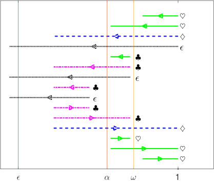
Figure 4.2: The various steps in ${\cal S}\setminus{\cal S}_{\|s\|}$ depending on intervals containing their origin $|x_{i,k}|$ and end $|x_{i,k}+s_{i,k}|$ points. The vertical lines show, in increasing order, $\epsilon$, $\alpha$ and $\omega$. The line type of the represented step indicates that it belongs to ${\cal S}_{\epsilon,k}$ (dotted), ${\cal S}_{\heartsuit,k}$ (solid), ${\cal S}_{\diamondsuit,k}$ (dashed) and ${\cal S}_{\clubsuit,k}$ (dash-dotted).The vertical axis is meaningless.

It is important to observe that the mechanism of the algorithm ensures that, once an $x_{i}$ falls in the interval $[-\epsilon,\epsilon]$ at iteration $k$, it never leaves it (and essentially “drops out” of the calculation). Thus there are no right-oriented dotted steps in Figure 4.2 and also

$$|{\cal S}_{\epsilon}|\leq|{\cal H}|.$$ (4.42)

Moreover Lemma 4.8 ensures that ${\cal I}_{\clubsuit,k}=\emptyset$ for all $k\in{\cal S}$, and hence that

$$|{\cal S}_{\clubsuit}|=0.$$ (4.43)

As a consequence, one has that ${\cal S}_{\epsilon}$, ${\cal S}_{\|s\|}$, ${\cal S}_{\heartsuit}$, and ${\cal S}_{\diamondsuit}$ form a partition of ${\cal S}$. It is also easy to verify that, if $k\in{\cal S}_{\diamondsuit}$ and $i\in{\cal I}_{\diamondsuit,k}$, then

$$\|s_{k}\|\geq\|P_{{\cal R}_{\{i\}}}(s_{k})\|=|s_{i,k}|\geq\omega-\alpha={\scriptstyle\frac{1}{4}}\omega>0,$$ (4.44)

where we have used the contractive property of orthogonal projections.

We now show that the steps at iterations whose index is in ${\cal S}_{\heartsuit}$ are not too short.

Lemma 4.9

Suppose that AS.1-AS.3 and AS.5 hold, that $$\epsilon<\alpha$$ (4.45) and consider $k\in{\cal S}_{\heartsuit}$ before termination. Then $$\|s_{k}\|\geq(\kappa_{\heartsuit}\,\epsilon)^{\frac{1}{p}},$$ (4.46) where $$\kappa_{\heartsuit}\stackrel{{\scriptstyle\rm def}}{{=}}\left[2(L(\alpha)+\theta+\frac{\displaystyle|{\cal N}|}{\displaystyle p!}\,\varsigma_{\max}^{p+1}\,\sigma_{\max})\right]^{-1}.$$ (4.47)

• Proof.    Observe first that, since $k\in{\cal S}_{\heartsuit}\subseteq{\cal S}$, we have that $x_{k+1}=x_{k}+s_{k}$ and, because $\epsilon\leq\alpha$ and ${\cal C}_{k}^{+}\subseteq{\cal C}_{k}$, we deduce that ${\cal C}_{k}={\cal C}_{k}^{+}={\cal C}_{k+1}$ and ${\cal R}_{k}={\cal R}_{k}^{+}={\cal R}_{k+1}$. Moreover the definition of ${\cal S}_{\heartsuit}$ ensures that, for all $i\in{\cal H}\setminus{\cal C}_{k}$,

  $$\min\Big{[}|x_{i,k}|,|x_{i,k}+s_{i,k}|\Big{]}\geq\alpha.$$ (4.48)

  Hence

  $${\cal O}_{*}\stackrel{{\scriptstyle\rm def}}{{=}}{\cal O}_{k,\alpha}={\cal H}\setminus{\cal C}_{k}={\cal H}\setminus{\cal C}_{k}^{+},$$

  and thus

  $${\cal R}_{*}\stackrel{{\scriptstyle\rm def}}{{=}}{\cal R}_{k}={\cal R}_{k}^{+}\;\;\mbox{ and }\;\;{\cal W}_{*}\stackrel{{\scriptstyle\rm def}}{{=}}{\cal W}_{k}={\cal W}_{k}^{+}={\cal N}\cup{\cal O}_{*}.$$ (4.49)

  As a consequence the step computation must have been completed because (3.15) holds, which implies that

  $$\chi_{m}(x_{k},s_{k},\epsilon)=\chi_{m_{{\cal W}_{*}}}(x_{k},s_{k},\epsilon)=\left|\min_{{}_{\stackrel{{\scriptstyle\scriptstyle x_{k}+s_{k}+d\in{\cal F}}}{{\scriptstyle d\in{\cal R}_{*},\|d\|\leq 1}}}}\nabla_{s}m_{{\cal W}_{*}}(x_{k},s_{k})^{T}d\right|\leq\theta\|s_{k}\|^{p}.$$ (4.50)

  Observe also that (4.49), (4.5) with $\phi=\alpha$ (because $k\in{\cal S}_{\heartsuit}$) , (4.30) and (4.2) then imply that

  $$\begin{array}[]{lcl}\|\nabla_{x}^{1}f_{{\cal W}_{*}}(x_{k+1})-\nabla_{s}^{1}m_{{\cal W}_{*}}(x_{k},s_{k})\|&=&\|\nabla_{x}^{1}f_{{\cal N}\cup{\cal O}_{*}}(x_{k+1})-\nabla_{s}^{1}m_{{\cal N}\cup{\cal O}_{*}}(x_{k},s_{k})\|\\[12.91663pt] &\leq&L(\alpha)\|s_{k}\|^{p}+\frac{\displaystyle 1}{\displaystyle(p+1)!}\,\sigma_{\max}\displaystyle\sum_{i\in{\cal N}}\|\,\nabla_{s}^{1}\|s_{i,k}\|^{p+1}\,\|\\[12.91663pt] &\leq&L(\alpha)\|s_{k}\|^{p}+\frac{\displaystyle 1}{\displaystyle p!}\,\sigma_{\max}\displaystyle\sum_{i\in{\cal N}}\|s_{i,k}\|^{p}\\[12.91663pt] &\leq&L(\alpha)\|s_{k}\|^{p}+\frac{\displaystyle|{\cal N}|}{\displaystyle p!}\,\varsigma_{\max}^{p+1}\,\sigma_{\max}\|s_{k}\|^{p}\\[12.91663pt] &=&\left[L(\alpha)+\frac{\displaystyle|{\cal N}|}{\displaystyle p!}\,\varsigma_{\max}^{p+1}\,\sigma_{\max}\right]\|s_{k}\|^{p},\end{array}$$ (4.51)

  and also that

  $$\begin{array}[]{lcl}\chi_{f}(x_{k+1},\epsilon)&=&|\nabla_{x}^{1}f_{{\cal W}_{*}}(x_{k+1})[d_{k+1}]|\\[4.30554pt] &\leq&|\nabla_{x}^{1}f_{{\cal W}_{*}}(x_{k+1})[d_{k+1}]-\nabla_{s}^{1}m_{{\cal W}_{*}}(x_{k},s_{k})[d_{k+1}]|\\[4.30554pt] &&\hskip 28.45274pt+|\nabla_{s}^{1}m_{{\cal W}_{*}}(x_{k},s_{k})[d_{k+1}]|,\end{array}$$ (4.52)

  where the first equality defines the vector $d_{k+1}$ with

  $$\|d_{k+1}\|\leq 1.$$ (4.53)

  Assume now, for the purpose of deriving a contradiction, that

  $$\|s_{k}\|<\left[\frac{\chi_{f}(x_{k+1},\epsilon)}{2(L(\alpha)+\theta+\frac{\displaystyle|{\cal N}|}{\displaystyle p!}\,\varsigma_{\max}^{p+1}\,\sigma_{\max})}\right]^{\frac{1}{p}}$$ (4.54)

  at iteration $k\in{\cal S}_{\heartsuit}$. Using (4.53) and (4.51), we then obtain that

  $$\begin{array}[]{lcl}\lx@intercol\@ADDCLASS{ltx_eqn_lefteqn}$\displaystyle-\nabla_{x}^{1}f_{{\cal W}_{*}}(x_{k+1})[d_{k+1}]+\nabla_{s}^{1}m_{{\cal W}_{*}}(x_{k},s_{k})[d_{k+1}]$\mbox{}\hfil\lx@intercol\\[6.45831pt] &\leq&|\nabla_{x}^{1}f_{{\cal W}_{*}}(x_{k+1})[d_{k+1}]-\nabla_{s}^{1}m_{{\cal W}_{*}}(x_{k},s_{k})[d_{k+1}]|\\[6.45831pt] &=&|(\nabla_{x}^{1}f_{{\cal W}_{*}}(x_{k+1})-\nabla_{s}^{1}m_{{\cal W}_{*}}(x_{k},s_{k}))[d_{k+1}]|\\[6.45831pt] &\leq&\|\nabla_{x}^{1}f_{{\cal W}_{*}}(x_{k+1})-\nabla_{s}^{1}m_{{\cal W}_{*}}(x_{k},s_{k})\|\;\|d_{k+1}\|\\[6.45831pt] &<&(L(\alpha)+\frac{\displaystyle|{\cal N}|}{\displaystyle p!}\,\varsigma_{\max}^{p+1}\,\sigma_{\max})\|s_{k}\|^{p}.\end{array}$$ (4.55)

  From (4.54) and the first part of (4.52), we have that

  $$\begin{array}[]{lcl}-\nabla_{x}^{1}f_{{\cal W}_{*}}(x_{k+1})[d_{k+1}]+\nabla_{s}^{1}m_{{\cal W}_{*}}(x_{k},s_{k}))[d_{k+1}]&<&{\scriptstyle\frac{1}{2}}\chi_{f}(x_{k+1},\epsilon)\\[4.30554pt] &=&-{\scriptstyle\frac{1}{2}}\nabla_{x}^{1}f_{{\cal W}_{*}}(x_{k+1})[d_{k+1}],\end{array}$$

  which in turn ensures that

  $$\nabla_{s}^{1}m_{{\cal W}_{*}}(x_{k},s_{k})[d_{k+1}]<{\scriptstyle\frac{1}{2}}\nabla_{x}^{1}f_{{\cal W}_{*}}(x_{k+1})[d_{k+1}]<0.$$

  Moreover, by definition of $\chi_{f}(x_{k+1},\epsilon)$,

  $$x_{k+1}+d_{k+1}\in{\cal F}\;\;\mbox{and}\;\;d_{k+1}\in{\cal R}_{k+1}={\cal R}_{k}^{+}.$$

  Hence, using (3.16) and (4.53),

  $$|\nabla_{s}^{1}m_{{\cal W}_{*}}(x_{k},s_{k})[d_{k+1}]|\leq\chi_{m_{{\cal W}_{*}}}(x_{k},s_{k},\epsilon).$$ (4.56)

  We may then substitute this inequality in (4.52) to deduce as above that

  $$\begin{array}[]{lcl}\chi_{f}(x_{k+1})&\leq&|\nabla_{x}^{1}f_{{\cal W}_{*}}(x_{k+1})[d_{k+1}]-\nabla_{s}^{1}m_{{\cal W}_{*}}(x_{k},s_{k})[d_{k+1}]|+\chi_{m_{{\cal W}_{*}}}(x_{k},s_{k},\epsilon)\\[8.61108pt] &\leq&(L(\alpha)+\theta+\frac{\displaystyle|{\cal N}|}{\displaystyle p!}\,\varsigma_{\max}^{p+1}\,\sigma_{\max})\|s_{k}\|^{p}\end{array}$$ (4.57)

  where the last inequality results from (4.55), the identity $x_{k+1}=x_{k}+s_{k}$ and (4.50). But this contradicts our assumption that (4.54) holds. Hence (4.54) must fail. The inequality (4.46) then follows by combining this conclusion with the fact that $\chi_{f}(x_{k+1},\epsilon)>\epsilon$ before termination. $\Box$

We are now ready to consider our first complexity result, whose proof uses restrictions of the successful and unsuccessful iteration index sets defined above to $\{0,\ldots,k\}$, which are given by

$${\cal S}_{k}\stackrel{{\scriptstyle\rm def}}{{=}}\{0,\ldots,k\}\cap{\cal S},\;\;\;\;{\cal U}_{k}\stackrel{{\scriptstyle\rm def}}{{=}}\{0,\ldots,k\}\setminus{\cal S}_{k},$$ (4.58)

respectively.

Theorem 4.10

Suppose that AS.1-AS.5 hold and that $$\epsilon\leq\left[\alpha,\left({\scriptstyle\frac{1}{4}}\omega\kappa_{\heartsuit}^{-\frac{1}{p+1}}\right)^{p}\right]\;\;\mbox{ if }\;\;{\cal H}\neq\emptyset.$$ (4.59) Then Algorithm 3.1 requires at most $$\kappa_{\cal S}(f(x_{0})-f_{\rm low})\epsilon^{-{\scriptstyle\frac{p+1}{p}}}+|{\cal H}|$$ (4.60) successful iterations to return a point $x_{\epsilon}\in{\cal F}$ such that $\chi_{f}(x_{\epsilon},\epsilon)\leq\epsilon$, for $$\kappa_{\cal S}=\frac{\displaystyle(p+1)!}{\displaystyle\eta\,\sigma_{\min}\,\varsigma_{\min}^{p+1}}\Big{[}2(L(\alpha)+\theta+\frac{\displaystyle|{\cal N}|}{\displaystyle p!}\,\varsigma_{\max}^{p+1}\,\gamma_{2})\Big{]}^{\frac{p+1}{p}}.$$ (4.61)

• Proof.    Let $k\in{\cal S}$ be index of a successful iteration before termination, and suppose first that ${\cal H}\neq\emptyset$. Because the iteration is successful, we obtain, using AS.4 and Lemma 4.3, that

  $$f(x_{0})-f_{\rm low}\geq f(x_{0})-f(x_{k+1})\geq\displaystyle\sum_{\ell\in{\cal S}_{k}}\Big{[}f(x_{\ell})-f(x_{\ell}+s_{\ell})\Big{]}\geq\eta\displaystyle\sum_{\ell\in{\cal S}_{k}}\Big{[}f(x_{\ell})-T_{f,p}(x_{\ell},s_{\ell})\Big{]}.$$ (4.62)

  In addition to (4.58), let us define

  $${\cal S}_{\epsilon,k}\stackrel{{\scriptstyle\rm def}}{{=}}\{0,\ldots,k\}\cap{\cal S}_{\epsilon},\;\;\;\;{\cal S}_{\|s\|,k}\stackrel{{\scriptstyle\rm def}}{{=}}\{0,\ldots,k\}\cap{\cal S}_{\|s\|},$$ (4.63)

  $${\cal S}_{\heartsuit,k}\stackrel{{\scriptstyle\rm def}}{{=}}\{0,\ldots,k\}\cap{\cal S}_{\heartsuit},\;\;\;\;{\cal S}_{\diamondsuit,k}\stackrel{{\scriptstyle\rm def}}{{=}}\{0,\ldots,k\}\cap{\cal S}_{\diamondsuit}.$$

  We now use the fact that ${\cal S}_{\|s\|,k}\cup{\cal S}_{\heartsuit,k}\cup{\cal S}_{\diamondsuit,k}={\cal S}_{k}\setminus{\cal S}_{\epsilon,k}\subseteq{\cal S}_{k}$, and (4.2) to deduce from (4.62) that

  $$\begin{array}[]{lcl}f(x_{0})-f_{\rm low}&\geq&\eta\left\{\displaystyle\sum_{\ell\in{\cal S}_{\|s\|,k}}\Big{[}f(x_{\ell})-T_{f,p}(x_{\ell},s_{\ell})\Big{]}+\displaystyle\sum_{\ell\in{\cal S}_{\heartsuit,k}}\Big{[}f(x_{\ell})-T_{f,p}(x_{\ell},s_{\ell})\Big{]}\right.\\[17.22217pt] &&\hskip 28.45274pt+\left.\displaystyle\sum_{\ell\in{\cal S}_{\diamondsuit,k}}\Big{[}f(x_{\ell})-T_{f,p}(x_{\ell},s_{\ell})\Big{]}\right\}\\[17.22217pt] &\geq&\frac{\displaystyle\eta\sigma_{\min}}{\displaystyle(p+1)!}\left\{|{\cal S}_{\|s\|,k}|\displaystyle\min_{\ell\in{\cal S}_{\|s\|,k}}\left[\displaystyle\sum_{i\in{\cal N}}\|s_{i,\ell}\|^{p+1}\right]+|{\cal S}_{\heartsuit,k}|\displaystyle\min_{\ell\in{\cal S}_{\heartsuit,k}}\left[\displaystyle\sum_{i\in{\cal N}}\|s_{i,\ell}\|^{p+1}\right]\right.\\[12.91663pt] &&\hskip 28.45274pt+\left.|{\cal S}_{\diamondsuit,k}|\displaystyle\min_{\ell\in{\cal S}_{\diamondsuit,k}}\left[\displaystyle\sum_{i\in{\cal N}}\|s_{i,\ell}\|^{p+1}\right]\right\}\\[12.91663pt] &\geq&\frac{\displaystyle\eta\sigma_{\min}\varsigma_{\min}^{p+1}}{\displaystyle(p+1)!}\left\{|{\cal S}_{\|s\|,k}|\displaystyle\min_{\ell\in{\cal S}_{\|s\|,k}}\|s_{\ell}\|^{p+1}+|{\cal S}_{\heartsuit,k}|\displaystyle\min_{\ell\in{\cal S}_{\heartsuit,k}}\|s_{\ell}\|^{p+1}\right.\\[12.91663pt] &&\hskip 28.45274pt+\left.|{\cal S}_{\diamondsuit,k}|\displaystyle\min_{\ell\in{\cal S}_{\diamondsuit,k}}\|s_{\ell}\|^{p+1}\right\}.\end{array}$$

  Because of of (4.40), (4.63), Lemma 4.9 and (4.44), this now yields that

  $$\begin{array}[]{lcl}f(x_{0})-f_{\rm low}&\geq&\frac{\displaystyle\eta\sigma_{\min}\varsigma_{\min}^{p+1}}{\displaystyle(p+1)!}\left\{|{\cal S}_{\|s\|,k}|+|{\cal S}_{\heartsuit,k}|(\kappa_{\heartsuit}\epsilon)^{\frac{p+1}{p}}+|{\cal S}_{\diamondsuit|,k}(\omega-\alpha)^{p+1}\right\}\\[12.91663pt] &\geq&\frac{\displaystyle\eta\sigma_{\min}\varsigma_{\min}^{p+1}}{\displaystyle(p+1)!}\Big{\{}|{\cal S}_{\|s\|,k}|+|{\cal S}_{\heartsuit,k}|+|{\cal S}_{\diamondsuit,k}|\Big{\}}\min\left[(\kappa_{\heartsuit}\epsilon)^{\frac{p+1}{p}},({\scriptstyle\frac{1}{4}}\omega)^{p+1}\right]\\[12.91663pt] &\geq&\frac{\displaystyle\eta\sigma_{\min}\varsigma_{\min}^{p+1}}{\displaystyle(p+1)!}\,|{\cal S}_{k}\setminus{\cal S}_{\epsilon}|\,(\kappa_{\heartsuit}\epsilon)^{\frac{p+1}{p}}\end{array}$$

  where we used (4.59), the partition of ${\cal S}_{k}\setminus{\cal S}_{\epsilon,k}$ in ${\cal S}_{\|s\|,k}\cup{\cal S}_{\heartsuit,k}\cup{\cal S}_{\diamondsuit,k}$ and the inequality ${\scriptstyle\frac{1}{4}}\omega<1$ to obtain the last inequality. Thus

  $$|{\cal S}_{k}|\leq\kappa_{\cal S}(f(x_{0})-f_{\rm low})\epsilon^{-\frac{p+1}{p}}+|{\cal S}_{\epsilon,k}|,$$ (4.64)

  where $\kappa_{\cal S}$ is given by (4.61). The desired iteration complexity (4.60) then follows from this bound, $|{\cal S}_{\epsilon,k}|\leq|{\cal S}_{\epsilon}|$ and (4.42). $\Box$

To complete our analysis in terms of evaluations rather than successful iterations, we need to bound the total number of all (successful and unsuccessful) iterations.

Lemma 4.11

Assume that AS.2 and AS.3 hold. Then, for all $k\geq 0$, $$k\leq\kappa^{a}|{\cal S}_{k}|+\kappa^{b},$$ where $$\kappa^{a}\stackrel{{\scriptstyle\rm def}}{{=}}1+\frac{|{\cal N}|\,|\log\gamma_{0}|}{\log\gamma_{1}}\;\;\mbox{ and }\;\;\kappa^{b}\stackrel{{\scriptstyle\rm def}}{{=}}\frac{|{\cal N}|}{\log\gamma_{1}}\log\left(\frac{\sigma_{\max}}{\sigma_{\min}}\right).$$

• Proof.    For $i\in{\cal N}$, define

  $${\cal J}_{i,k}\stackrel{{\scriptstyle\rm def}}{{=}}\{j\in\{0,\ldots,k\}\mid\mbox{(\ref{sig-incr}) holds with }k\leftarrow j\},$$

  (the set of iterations where $\sigma_{i,j}$ is increased) and

  $${\cal D}_{i,k}\stackrel{{\scriptstyle\rm def}}{{=}}\{j\in\{0,\ldots,k\}\mid\mbox{(\ref{sig-decr}) holds with }k\leftarrow j\}\subseteq{\cal S}_{k}$$

  (the set of iterations where $\sigma_{i,j}$ in decreased), the final inclusion resulting from the condition that $\rho_{k}\geq\eta$ in both (3.21) and (3.22). Observe also that the mechanism of the algorithm, the fact that $\gamma_{0}\in(0,1)$ and Lemma 4.6 impose that, for each $i\in{\cal N}$,

  $$\sigma_{\min}\gamma_{1}^{|{\cal J}_{i,k}|}\gamma_{0}^{|{\cal S}_{k}|}\leq\sigma_{i,0}\gamma_{1}^{|{\cal J}_{i,k}|}\gamma_{0}^{|{\cal D}_{i,k}|}\leq\sigma_{i,k}\leq\sigma_{\max}.$$

  Dividing by $\sigma_{\min}>0$ and taking logarithms yields that, for all $i\in{\cal N}$ and all $k>0$,

  $$|{\cal J}_{i,k}|\log\gamma_{1}+|{\cal S}_{k}|\log\gamma_{0}\leq\log\left(\frac{\sigma_{\max}}{\sigma_{\min}}\right).$$ (4.65)

  Note now that, if (3.19) fails for all $i\in{\cal N}$ and given that Lemma 4.4 ensures that $f_{i}(x_{i}+s_{i})\leq m_{i}(x_{i},s_{i})$ for $i\in{\cal H}\setminus{\cal C}_{k}^{+}$, then

  $$\delta f_{k}=\sum_{i\in{\cal W}_{k}^{+}}\delta f_{i,k}\geq\sum_{i\in{\cal W}_{k}^{+}}\delta m_{i,k}=\delta m_{k}.$$

  Thus, in view of (3.18), we have that $\rho_{k}\geq 1>\eta$ and iteration $k$ is successful. Thus, if iteration $k$ is unsuccessful, $\sigma_{i,k}$ is increased with (3.20) for at least one $i\in{\cal N}$. Hence we deduce that

  $$|{\cal U}_{k}|\leq\sum_{i\in{\cal N}}|{\cal J}_{i,k}|\leq|{\cal N}|\,\max_{i\in{\cal N}}|{\cal J}_{i,k}|.$$ (4.66)

  The desired bound follows from (4.65) and (4.66) by using the fact that $k=|{\cal S}_{k}|+|{\cal U}_{k}|-1\leq|{\cal S}_{k}|+|{\cal U}_{k}|$, the term -1 in the equality accounting for iteration 0. $\Box$

We may now state our main evaluation complexity result.

Theorem 4.12

Suppose that AS.1, (1.3), AS.2-AS.5 and (4.59) hold. Then Algorithm 3.1 using models (3.12) for $i\in{\cal H}$ requires at most $$\kappa^{a}\left[\kappa_{\cal S}(f(x_{0})-f_{\rm low})\epsilon^{-{\scriptstyle\frac{p+1}{p}}}+|{\cal H}|\right]+\kappa^{b}+1$$ (4.67) iterations and evaluations of $f$ and its first $p$ derivatives to return a point $x_{\epsilon}\in{\cal F}$ such that $\chi_{f}(x_{\epsilon},\epsilon)\leq\epsilon$.

• Proof.    If termination occurs at iteration 0, the theorem obviously holds. Assume therefore that termination occurs at iteration $k+1$, in which case there must be at least one successful iteration. We may therefore deduce the desired bound from Theorem 4.10, Lemma 4.11 and the fact that each successful iteration involves the evaluation of $f(x_{k})$ and $\{\nabla_{x}^{i}f_{{\cal W}_{k}}(x_{k})\}_{i=1}^{p}$, while each unsuccessful iteration only involves that of $f(x_{k})$ and $\nabla_{x}^{1}f_{{\cal W}_{k}}(x_{k})$. $\Box$

Note that we may count derivatives’ evaluations in Theorem 4.12 because only the derivatives of $f_{{\cal W}_{k}}$ are ever evaluated, and these are well-defined. For completeness, we state the complexity bound of the important purely Lipschitzian case.

Corollary 4.13

Suppose that AS.1-AS.4 hold and ${\cal H}=\emptyset$. Then Algorithm 3.1 requires at most $$\kappa^{a}\left[\kappa_{\cal S}(f(x_{0})-f_{\rm low})\epsilon^{-{\scriptstyle\frac{p+1}{p}}}\right]+\kappa^{b}+1$$ iterations and evaluations of $f$ and its first $p$ derivatives to return a point $x_{\epsilon}\in{\cal F}$ such that $$\chi_{f}(x_{\epsilon})\stackrel{{\scriptstyle\rm def}}{{=}}\left|\min_{{}_{\stackrel{{\scriptstyle\scriptstyle x+d\in{\cal F}}}{{\scriptstyle\|d\|\leq 1}}}}\nabla_{x}^{1}f_{{\cal W}(x)}(x)^{T}d\right|\leq\epsilon.$$

• Proof.   Directly follows from Theorem 4.12, ${\cal H}=\emptyset$ and the obesrvation that ${\cal R}(x,\epsilon)=\hbox{I\hskip-2.0ptR}^{n}$ for all $x\in{\cal F}$ since ${\cal C}(x,\epsilon)=\emptyset$. $\Box$

5 Evaluation complexity for general convex ${\cal F}$

The two-sided model (3.12) has clear advantages, the main ones being that, except at the origin where it is non-smooth, it is polynomial and has finite gradients (and higher derivatives) over each of its two branches. It is not however without drawbacks. The first of these is that its prediction for the gradient (and higher derivatives) is arbitrarily inaccurate as the origin is approached, the second being its evaluation cost which is typically higher than evaluating $|x+s|^{q}$ or its derivative directly. In particular, it is the first drawback that required the careful analysis of Lemma 4.5, in turn leading, via Lemma 4.7, to the crucial Lemma 4.8. This is significant because this last lemma, in addition to the use of (3.12) and the requirement that $p$ must be odd, also requires the ’kernel-centered’ assumption (1.3), a sometimes undesirable restriction of the feasible domain geometry.

In the case where evaluating $f_{\cal N}$ is very expensive and the convex ${\cal F}$ is not ’kernel-centered’, it may sometimes be acceptable to push the difficulty of handling the non-Lipschitzian nature of the $\ell_{q}$ norm regularization in the subproblem of computing $s_{k}$, if evaluations of $f_{\cal N}$ can be saved. In this context, a simple alternative is then to use

$$m_{i}(x_{i},s_{i})=|x_{i}+s_{i}|^{q}\;\;\mbox{for}\;\;i\in{\cal H}$$ (5.1)

that is $m_{i}(x_{i},s_{i})=f_{i}(x_{i}+s_{i})$ for $i\in{\cal H}$. The cost of finding a suitable step satisfying (3.15) may of course be increased, but, as we already noted, this cost is irrelevant for worst-case evaluation analysis as long as only the evaluation of $f_{\cal N}$ and its derivatives is taken into account. The choice (5.1) clearly maintains the overestimation property of Lemma 4.4. Moreover, it is easy to verify (using AS.3 and (5.1)) that

$$\|\nabla_{x}f_{{\cal W}_{k}^{+}}(x_{k}+s_{k})-\nabla_{s}^{1}m_{{\cal W}_{k}^{+}}(x_{k},s_{k})\|=\|\nabla_{x}f_{\cal N}(x_{k}+s_{k})-\nabla_{s}^{1}m_{\cal N}(x_{k},s_{k})\|\leq L_{\max}\|s_{k}\|^{p}.$$ (5.2)

This in turn implies that the proof of Lemma 4.9 can be extended without requiring (4.48) and using ${\cal O}_{*}={\cal H}\setminus{\cal C}_{k}^{+}$. The derivation of (4.51) then simplifies because of (5.2) and holds for all $i\in{\cal H}\setminus{\cal C}_{k}^{+}$ with $L(\alpha)=L_{\max}$, so that (4.46) holds for all $k\in{\cal S}$, the assumption (4.45) being now irrelevant. This result then implies that the distinction made between ${\cal S}_{\heartsuit}$, ${\cal S}_{\diamondsuit}$, $S\cal_{\clubsuit}$ and ${\cal S}_{\|s\|}$ is unecessary because (4.46) holds for all $k\in{\cal S}={\cal S}_{\heartsuit}$. Moreover, since we no longer need Lemma 4.8 to prove that ${\cal S}_{\clubsuit}=\emptyset$, we no longer need the restrictions that $p$ is odd and (1.3) either. As consequence, we deduce that Theorem 4.10 holds for arbitrary $p\geq 1$ and for arbitrary convex, closed non-empty ${\cal F}$, without the need to assume (4.59) and with $L(\alpha)$ replaced by $L_{\max}$ in (4.61). Without altering Lemma 4.11, we may therefore deduce the following complexity result.

Theorem 5.1

Suppose that AS.1, AS.2 (without the restriction that $p$ must be odd), AS.3 and AS.4 hold. Then Algorithm 3.1 using the true models (5.1) for $i\in{\cal H}$ requires at most $$\kappa^{a}\left[\kappa_{\cal S}^{\rm true}(f(x_{0})-f_{\rm low})\epsilon^{-{\scriptstyle\frac{p+1}{p}}}+|{\cal H}|\right]+\kappa^{b}+1$$ iterations and evaluations of $f_{\cal N}$ and its first $p$ derivatives to return a point $x_{\epsilon}\in{\cal F}$ such that $\chi_{f}(x_{\epsilon},\epsilon)\leq\epsilon$, where $$\kappa_{\cal S}^{\rm true}=\frac{\displaystyle(p+1)!}{\displaystyle\eta\,\sigma_{\min}\,\varsigma_{\min}^{p+1}}\Big{[}2|{\cal N}|\varsigma^{p+1}\left(L+\theta+\frac{\displaystyle\gamma_{2}}{\displaystyle p!}\right)\Big{]}^{\frac{p+1}{p}}.$$

As indicated, the complexity is expressed in this theorem in terms of evaluations of $f_{\cal N}$ and its derivatives only. The evaluation count for the terms $f_{i}$ ($i\in{\cal H}$) may be higher since these terms are evaluated in computing the step $s_{k}$ using the models (5.1). Note that the difficulty of handling infinite derivatives is passed on to the subproblem solver in this approach.

Moreover, it also results from the analysis in this section that one may consider objective functions of the form

$$f(x)=f_{\cal N}(x)+f_{\cal H}(x)$$

and prove an $O(\epsilon^{-\frac{p+1}{p}})$ evaluation compexity bound if $f_{\cal N}$ has Lipschitz continuous derivatives of order $p$ and if $m_{\cal H}(x_{k},s)=f_{\cal H}(x_{k}+s)$, passing all difficulties associated with $f_{\cal H}$ to the subproblem of computing the step $s_{k}$.

As it turns out, an evaluation complexity bound may also be computed if one insist on using the Taylor’s models (3.12) while allowing the feasible set to be an arbitrary convex, closed and non-empty set. Not surprisingly, the bound is (significantly) worse than that provided by Theorem 4.12, but has the merit of existing. Its derivation is based on the observation that (4.14) in Lemma 4.4 and (4.21) imply that, for $i\in{\cal H}\setminus{\cal C}_{k}^{+}$,

$$|\nabla_{s_{i}}^{1}|x_{i}+s_{i}|^{q}-\nabla_{s_{i}}^{1}m_{i}(x_{i},s_{i})|\leq q\left(\min\Big{[}|x_{i}|,|x_{i}+s_{i}|\Big{]}\right)^{q-p-1}|\mu(x_{i},s_{i})|^{p}\leq q\epsilon^{q-p-1}|s_{i}|^{p}.$$ (5.3)

This bound can then be used in a variant of Lemma 4.9 just like (5.2) was in Section 5. In the updated version of Lemma 4.9, we replace $L(\alpha)$ by

$$L_{*}\stackrel{{\scriptstyle\rm def}}{{=}}|{\cal N}|\,\varsigma_{\max}^{p}\,L_{\max}+|{\cal H}|\,\varsigma_{\max}^{p}\,q$$

and (4.51) now becomes

$$\|\nabla_{x}^{1}f_{{\cal W}_{k}^{+}}(x_{k+1})-\nabla_{s}^{1}m_{{\cal W}_{k}^{+}}(x_{k},s_{k})\|\leq\left[L_{*}\epsilon^{q-p-1}+\frac{\displaystyle|{\cal N}|}{\displaystyle p!}\varsigma^{p}\sigma_{\max}\right]\|s_{k}\|^{p}.$$

This results in replacing (4.57) by

$$\chi_{f}(x_{k+1})\leq(L_{*}\epsilon^{q-p-1}+\theta+\frac{\displaystyle|{\cal N}|}{\displaystyle p!}\,\varsigma_{\max}^{p+1}\,\sigma_{\max})\|s_{k}\|^{p}\leq(L_{*}+\theta+\frac{\displaystyle|{\cal N}|}{\displaystyle p!}\,\varsigma_{\max}^{p+1}\,\sigma_{\max})\epsilon^{q-p-1}\|s_{k}\|^{p}$$ (5.4)

and therefore (4.46) is replaced by

$$\|s_{k}\|\geq\left[2\left(L_{*}+\theta+\frac{\displaystyle|{\cal N}|}{\displaystyle p!}\,\varsigma_{\max}^{p+1}\,\sigma_{\max}\right)\right]^{-\frac{1}{p}}\epsilon^{\frac{p+2-q}{p}}.$$

We may now follow the steps leading to Theorem 5.1 and deduce a new complexity bound.

Theorem 5.2

Suppose that AS.1–AS.4 hold. Then Algorithm 3.1 using the Taylor models (3.12) for $i\in{\cal H}$ requires at most $$\kappa^{a}\left[\kappa_{\cal S}^{*}(f(x_{0})-f_{\rm low})\epsilon^{-{\scriptstyle\frac{(p+2-q)(p+1)}{p}}}+|{\cal H}|\right]+\kappa^{b}+1$$ iterations and evaluations of $f$ and its first $p$ derivatives to return a point $x_{\epsilon}\in{\cal F}$ such that $\chi_{f}(x_{\epsilon},\epsilon)\leq\epsilon$, where $$\kappa_{\cal S}^{*}=\frac{\displaystyle(p+1)!}{\displaystyle\eta\,\sigma_{\min}\,\varsigma_{\min}^{p+1}}\Big{[}2\left(L_{*}+\theta+\frac{\displaystyle|{\cal N}|}{\displaystyle p!}\,\varsigma_{\max}^{p+1}\,\gamma_{2}\right)\Big{]}^{\frac{p+1}{p}}.$$

Observe that, due to the second inequality of (5.4), $\theta$ can be replaced in (3.15) by $\theta_{*}=\theta\epsilon^{q-p-1}$, making the termination condition for the step computation very weak.

6 Further discussion

The above results suggest some additional comments.

• The complexity result in $O(\epsilon^{-(p+1)/p})$ evaluations obtained in Theorem 4.12 is identical in order to that presented in [3] for the unstructured unconstrained and in [9] for the unstructured convexly constrained cases. It is remarkable that incorporating non-Lipschitzian singularities in the objective function does not affect the worst-case evaluation complexity of finding an $\epsilon$-approximate first-order critical point.

• Interestingly, Corollary 4.13 also shows that using partially separable structure does not affect the evaluation complexity either, therefore allowing cost-effective use of problem structure with high-order models.

• The algorithm presented here is considerably simpler than that discussed in [16, 18] in the context of structured trust-regions. In addition, the present assumptions are also weaker. Indeed, an additional condition on long steps (see AA.1s in [18, p.364]) is no longer needed.

• Can one use even order models with Taylor models in the present framework? The main issue is that, when $p$ is even, the two-sided model $T_{|\cdot|^{q},p}(x_{i},s_{i})$ is no longer always an overestimate of $|x_{i}+s_{i}|^{q}$ when $|x_{i}+s_{i}|>|x_{i}|$, as can be verified from (4.14). While this can be taken care of by adding a regularization term to $m_{i}$, the necessary size of the regularization parameter may be unbounded when the iterates are sufficiently close from the singularity. This in turn destroys the good complexity because it forces the algorithm to take much too short steps.

  An alternative is to use mixed-orders models, that is models of even order ($p$, say) for the $f_{i}$ whose index is in ${\cal N}$ and odd order models for those with index in ${\cal H}$. However, this last (odd) order has to be at least as large as $p$, because it is the lowest order which dominates in the crucial Lemma 4.9 where the length is bounded below away from the singularity. The choice of a $(p+1)$-st order model for $i\in{\cal H}$ is then most natural.

• A variant of the algorithm can be stated where it is possible for a particular $x_{i}$ to leave the $\epsilon$-neighbourhood of zero, provided the associated step results in a significant (in view of Theorem 4.10) objective function decrease, such as a multiple of $\epsilon^{(p+1)/p}$ or some $\epsilon$-independent constant. These decreases can then be counted separately in the argument of Theorem 4.10 and cycling is impossible since there can be only a finite number of such decreases.

7 Conclusions

We have considered the problem of minimizing a partially-separable nonconvex objective function $f$ involving non-Lipschitzian $q$-norm regularization terms and subject to general convex constraints. Problems of this type are important in many areas, including data compression, image processing and bioinformatics. We have shown that the introduction of the non-Lipschitzian singularities and the exploitation of problem structure do not affect the worst-case evaluation complexity. More precisely, we have first defined $\epsilon$-approximate first-order critical points for the considered class of problems in a way that make the obtained complexity bounds comparable to existing results for the purely Lipschitzian case. We have then shown that, if $p$ is the (odd) degree of the models used by the algorithm, if the feasible set is ’kernel-centered’ and if Taylor models are used for the $q$-norm regularization terms, the bound of $O(\epsilon^{-\frac{p+1}{p}})$ evaluations of $f$ and its relevant derivatives (derived for the Lipschitzian case in [9]) is preserved in the presence of non-Lipschitzian singularities. In addition, we have shown that partially-separable structure present in the problem can be exploited (especially for high degree derivative tensors) without affecting the evaluation complexity either. We have also shown that, if the difficulty of handling the non-Lipschitzian regularization terms is passed to the subproblem (which can be meaningfull if evaluating the other parts of the objective function is very expensive) in that non-Lipschitz models are used for these terms, then the same bounds hold in terms of evaluation of the expensive part of the objective function, without the restriction that the feasible set be ‘kernel-centered’. A worse complexity bound has finally been provided in the case where one uses Taylor models for the $q$-norm regularization terms with a general convex feasible set.

These objectives have been attained by introducing a new first-order criticality measure as well as the new two-sided model of the singularity given by (3.11), which exploits the inherent symmetry and provides a useful overestimate of the $|x|^{q}$ if its order is chosen odd, without the need for smoothing functions.

References

[1]
W. Bian and X. Chen.
Linearly constrained non-Lipschitzian optimization for image
restoration.
SIAM Journal on Imaging Sciences, 8:2294–2322, 2015.
[2]
W. Bian and X. Chen.
Optimality and complexity for constrained optimization problems with
nonconvex regularization.
Mathematics of Operations Research, (to appear), 2017.
[3]
E. G. Birgin, J. L. Gardenghi, J. M. Martínez, S. A. Santos, and Ph. L.
Toint.
Worst-case evaluation complexity for unconstrained nonlinear
optimization using high-order regularized models.
Mathematical Programming, Series A, 163(1):359–368, 2017.
[4]
A.M. Bruckstein, D.L. Donoho, and M. Elad.
From sparse solutions of systems of equations to sparse modeling of
signals and images.
SIAM Review, 51:34–81, 2009.
[5]
C. Cartis, N. I. M. Gould, and Ph. L. Toint.
On the complexity of steepest descent, Newton’s and regularized
Newton’s methods for nonconvex unconstrained optimization.
SIAM Journal on Optimization, 20(6):2833–2852, 2010.
[6]
C. Cartis, N. I. M. Gould, and Ph. L. Toint.
Adaptive cubic overestimation methods for unconstrained optimization.
Part I: motivation, convergence and numerical results.
Mathematical Programming, Series A, 127(2):245–295, 2011.
[7]
C. Cartis, N. I. M. Gould, and Ph. L. Toint.
Adaptive cubic overestimation methods for unconstrained optimization.
Part II: worst-case function-evaluation complexity.
Mathematical Programming, Series A, 130(2):295–319, 2011.
[8]
C. Cartis, N. I. M. Gould, and Ph. L. Toint.
An adaptive cubic regularization algorithm for nonconvex optimization
with convex constraints and its function-evaluation complexity.
IMA Journal of Numerical Analysis, 32(4):1662–1695, 2012.
[9]
C. Cartis, N. I. M. Gould, and Ph. L. Toint.
Second-order optimality and beyond: characterization and evaluation
complexity in convexly-constrained nonlinear optimization.
Foundations of Computational Mathematics, (submitted),
2016.
[10]
L. Chen, N. Deng, and J. Zhang.
A trust region method with partial-update technique for unary
optimization.
In D. Z. Du, X. S. Zhang, and K. Cheng, editors, Operations
Research and Its Applications. Proceedings of the First International
Symposium, ISORA ’95, pages 40–46, Beijing, 1995. Beijing World Publishing.
[11]
L. Chen, N. Deng, and J. Zhang.
Modified partial-update Newton-type algorithms for unary
optimization.
Journal of Optimization Theory and Applications,
97(2):385–406, 1998.
[12]
X. Chen, D. Ge, and Y. Ye.
Complexity of unconstrained - minimization.
Mathematical Programming, Series A, 143:371–383, 2014.
[13]
X. Chen, L. Guo, Z. Lu, and J.J. Ye.
An augmented Lagrangian method for non-Lipschitz nonconvex
programming.
SIAM Journal on Numerical Analysis, 55:168–193, 2017.
[14]
X. Chen, L. Niu, and Y. Yuan.
Optimality conditions and smoothing trust region Newton method for
non-Lipschitz optimization.
SIAM Journal on Optimization, 23:1528–1552, 2013.
[15]
X. Chen, F. Xu, and Y. Ye.
Lower bound theory of nonzero entries in solutions of
- minimization.
SIAM Journal on Scientific Computing, 32:2832–2852, 2010.
[16]
A. R. Conn, N. I. M. Gould, A. Sartenaer, and Ph. L. Toint.
Convergence properties of minimization algorithms for convex
constraints using a structured trust region.
SIAM Journal on Optimization, 6(4):1059–1086, 1996.
[17]
A. R. Conn, N. I. M. Gould, and Ph. L. Toint.
LANCELOT: a Fortran package for large-scale nonlinear
optimization (Release A).
Number 17 in Springer Series in Computational Mathematics. Springer
Verlag, Heidelberg, Berlin, New York, 1992.
[18]
A. R. Conn, N. I. M. Gould, and Ph. L. Toint.
Trust-Region Methods.
MPS-SIAM Series on Optimization. SIAM, Philadelphia, USA, 2000.
[19]
R. Fourer, D. M. Gay, and B. W. Kernighan.
AMPL: A mathematical programming language.
Computer science technical report, AT&T Bell Laboratories, Murray
Hill, USA, 1987.
[20]
D. M. Gay.
Automatically finding and exploiting partially separable structure in
nonlinear programming problems.
Technical report, Bell Laboratories, Murray Hill, New Jersey, USA,
1996.
[21]
D. Goldfarb and S. Wang.
Partial-update Newton methods for unary, factorable and partially
separable optimization.
SIAM Journal on Optimization, 3(2):383–397, 1993.
[22]
N. I. M. Gould, J. Hogg, T. Rees, and J. Scott.
Solving nonlinear least-squares problems.
Technical report, Rutherford Appleton Laboratory, Chilton, England,
2016.
[23]
N. I. M. Gould, D. Orban, and Ph. L. Toint.
CUTEst: a constrained and unconstrained testing environment
with safe threads for mathematical optimization.
Computational Optimization and Applications, 60(3):545–557,
2015.
[24]
N. I. M. Gould and Ph. L. Toint.
FILTRANE, a Fortran 95 filter-trust-region package for
solving systems of nonlinear equalities, nonlinear inequalities and nonlinear
least-squares problems.
ACM Transactions on Mathematical Software, 33(1):3–25, 2007.
[25]
A. Griewank.
The modification of Newton’s method for unconstrained optimization
by bounding cubic terms.
Technical Report NA/12, Department of Applied Mathematics and
Theoretical Physics, University of Cambridge, Cambridge, United Kingdom,
1981.
[26]
A. Griewank and Ph. L. Toint.
On the unconstrained optimization of partially separable functions.
In M. J. D. Powell, editor, Nonlinear Optimization 1981, pages
301–312, London, 1982. Academic Press.
[27]
J. Huang, J.L. Horowitz, and S. Ma.
Asymptotic properties of bridge estimators in sparse highdimensional
regression models.
Annals of Statistics, 36:587–613, 2018.
[28]
Y.F. Liu, S. Ma, Y.H. Dai, and S. Zhang.
A smoothing SQP framework for a class of composite
minimization over polyhedron.
Mathematical Programming, Series A, 158:467–500, 2016.
[29]
Z. Lu.
Iterative reweighted minimization methods for regularized
unconstrained nonlinear programming.
Mathematical Programming, Series A, 147:277–307, 2014.
[30]
J. Mareček, P. Richtárik, and M. Takáč.
Distributed block coordinate descent for minimizing partially
separable functions.
Technical report, Department of Mathematics and Statistics,
University of Edinburgh, Edinburgh, Scotland, 2014.
[31]
Yu. Nesterov.
Introductory Lectures on Convex Optimization.
Applied Optimization. Kluwer Academic Publishers, Dordrecht, The
Netherlands, 2004.
[32]
Yu. Nesterov and B. T. Polyak.
Cubic regularization of Newton method and its global performance.
Mathematical Programming, Series A, 108(1):177–205, 2006.
[33]
J. S. Shahabuddin.
Structured trust-region algorithms for the minimization of
nonlinear functions.
PhD thesis, Department of Computer Science, Cornell University,
Ithaca, New York, USA, 1996.