Asymptotic Counting
in
Conformal Dynamical Systems

Abstract.

In this monograph we consider the general setting of conformal graph directed Markov systems modeled by countable state symbolic subshifts of finite type. We deal with two classes of such systems: attracting and parabolic. The latter being treated by means of the former.

We prove fairly complete asymptotic counting results for multipliers and diameters associated with preimages or periodic orbits ordered hy a natural geometric weighting. We also prove the corresponding Central Limit Theorems describing the further features of the distribution of their weights.

These results have direct applications to a variety of examples, including the case of Apollonian Circle Packings, Apollonian Triangle, expanding and parabolic rational functions, Farey maps, continued fractions, Mannenville-Pomeau maps, Schottky groups, Fuchsian groups, and many more. A fairly complete collection of asymptotic counting results for them is presented.

Our new approach is founded on spectral properties of complexified Ruelle–Perron–Frobenius operators and Tauberian theorems as used in classical problems of prime number theory.

1. Introduction

1.1. Short General Introduction

We begin with a simple problem formulated for iterated function systems (schemes). Let

$$\varphi_{e}:X\to X,\ \ e\in E,$$

be a countable, either finite or infinite, family of $C^{1+\alpha}$ contracting maps. We can associate to a point $\xi\in X$ the images

$$\varphi_{\omega}(\xi):=\varphi_{\omega_{1}}\circ\cdots\circ\varphi_{\omega_{n}}(\xi)$$

where $\omega_{i}\in E$, and then we associate two natural weights

$$\lambda_{\xi}(\omega):=-\log|(\varphi_{\omega})^{\prime}(\xi)|$$

and

$$\Delta_{\xi}(\omega):=-\log\text{\rm{diam}}(\varphi_{\omega}(X)).$$

Since there is no obvious way to order and count these images in terms of their combinatorial weight (the length of $\omega=(\omega_{1},\cdots,\omega_{n})$) we use instead the two weights introduced above: $\lambda_{\xi}(\omega)$ and $\Delta_{\xi}(\omega)$.

Under mild natural hypotheses we show that there exist two constants $C_{1},C_{2}>0$ (we provide explicit dynamical expressions for them) and $\delta\in(0,+\infty)$ such that

$$\lim_{T\to+\infty}\frac{\#\{\omega\hbox{ : }\lambda_{\xi}(\omega)\leq T\}}{e^{\delta T}}=C_{1}$$

and

$$\lim_{T\to+\infty}\frac{\#\{\omega\hbox{ : }\Delta_{\xi}(\omega)\leq T\}}{e^{\delta T}}=C_{2}.$$

These are the most transparent and simplest highlights of our results; but we prove more. For example, we provide the corresponding asymptotic results when in addition one requires that the points $\varphi_{\omega}(\xi)$ are to fall into a prescribed Borel subset $B$ of $X$. We also count multipliers and diameters if the points $\varphi_{\omega}(\xi)$ are replaced by periodic points of the system, i.e. by fixed points $x_{\omega}$ of the maps $\varphi_{\omega}$. We denote

$$\lambda_{p}(\omega)=-\log|(\varphi_{\omega})^{\prime}(x_{\omega})|.$$

A fuller description of our results is provided below in further subsections of this introduction and in complete detail in appropriate technical sections of the manuscript.

There are natural and instructive parallels of our work and the classical approach to the prime number theorem, as well as with known results on the Patterson-Sullivan orbit counting technology and the asymptotics of Apollonian circles. There are also applications to both expanding and parabolic rational functions, complex continued fractions, Farey maps, Mannenville-Pomeau maps, Schottky groups, Fuchsian groups, including Hecke groups, and more examples. We apply our general results to all of them, thus giving a unified approach which yields both new results and a new approach to established results.

All of these are based on our results for conformal graph directed Markov systems over a countable alphabet. Our counting results (on the symbolic level) are close in spirit to those of Steve Lalley from [25]. These would directly apply to our counting on the symbolic level if the graph directed Markov systems we considered had finite alphabets. However, we need to deal with those systems with a countable alphabet and we obtain our counting results via the study of spectral properties of complexified Ruelle–Perron–Frobenius operators, as used by William Parry and the first–named author, rather than the renewal theory approach of Lalley. It is worth mentioning that our results on the symbolic level could have been formulated and proved with no real additional difficulties in terms of ergodic sums of summable Hölder continuous potentials rather than merely the functions $\lambda_{\xi}(\omega)$ from the next subsection.

We would also like to add that our work was partly inspired by counting results of Kontorovich and Oh for Apollonian packings from [24] (see also [38]–[40]), which in our monograph are recovered and ultimately follow from our more general results for conformal graph directed Markov systems. Nevertheless the level of generality our approach is still entirely different than that of Kontorovich and Oh. We have recently received an interesting preprint [20] of Byron Heersink where he studies the counting problems for the Farey map, Gauss map, and closed geodesics on the modular surface. We would also like to note that a part of the classical work of the first named author and William Parry (including [46], [47], [45], [44]) the method of the complex Perron–Frobenius operator to approach various counting problems in geometry and dynamics has been used by several authors including [42], [35], [48], [3].

We now discuss our results below in more detail.

1.2. Asymptotic Counting Results

In Sections 3 and 9 we recall from [32] the respective concepts of attracting and parabolic countable alphabet conformal graph directed Markov systems. This symbolic viewpoint is convenient for keeping track of the quantities we want to counting. Let $A$ be the associated transition matrix and $\pi_{\mathcal{S}}(\rho)\in X$ is a reference point coded by an infinite sequence $\rho$. Fix any Borel set $B\subset X$ then for $T>0$ we define:

$$N_{\rho}(B,T) :=\#\left\{\omega\in E_{\rho}^{*}\hbox{ : }\varphi_{\omega}(\pi_{\mathcal{S}}(\rho))\in B\hbox{ and }\lambda_{\rho}(\omega)\leq T\right\}$$

and

$$N_{p}(B,T) :=\#\left\{\omega\in E_{p}^{*}\hbox{ : }x_{\omega}\in B\hbox{ and }\lambda_{p}(\omega)\leq T\right\},$$

where

$$E_{\rho}^{*}:=\{\omega\in E_{A}^{*}:\omega\rho\in E_{A}^{*}\},$$

and

$$E_{p}^{*}=\{\omega\in E_{A}^{*}:A_{\omega_{|\omega|}\omega_{1}}=1\},$$

are finite words of symbols, i.e. we count the number of words $\omega\in E_{i}^{*}$ for which the weight $\lambda_{i}(\omega)$ doesn’t exceed $T$ and, additionally, the image $\varphi_{\omega}(\pi_{\mathcal{S}}(\rho))$ is in $B$ if $i=\rho$, or the fixed point $x_{\omega}$ of $\varphi_{\omega}$, is in $B$ if $i=p$. The following result comprises both Theorem 5.9 for attracting conformal GDMSs and Theorem 11.2 for parabolic systems. We refer the reader to the appropriate sections for the detailed definitions of any unfamiliar hypotheses (or to the next subsection for concrete examples where these are known to hold).

Theorem 1.1 (Asymptotic Equidistribution Formula for Multipliers).

Suppose that $\mathcal{S}$ is either a strongly regular finitely irreducible D-generic attracting conformal GDMS or finite alphabet parabolic conformal GDMS.

Fix $\rho\in E_{A}^{\infty}$. If $B\subset X$ is a Borel set such that $\widetilde{m}_{\delta}(\partial B)=0$ (equivalently $\widetilde{\mu}_{\delta}(\partial B)=0$) then,

$$\lim_{T\to+\infty}\frac{N_{\rho}(B,T)}{e^{\delta T}}=\frac{\psi_{\delta}(\rho)}{\delta\chi_{\mu_{\delta}}}\widetilde{m}_{\delta}(B)$$

and

$$\lim_{T\to+\infty}\frac{N_{p}(B,T)}{e^{\delta T}}=\frac{1}{\delta\chi_{\mu_{\delta}}}\widetilde{\mu}_{\delta}(B).$$

Here we use the following notation.

• $\delta=\text{{\rm HD}}(J_{\mathcal{S}})$ is the Hausdorff dimension of the limit set (attractor) of the GDMS $\mathcal{S}$.

• $\widetilde{m}_{\delta}$ is the $\delta$-conformal measure for $\mathcal{S}$.

• $\widetilde{\mu}_{\delta}$ is its $\mathcal{S}$–invariant version.

• $\psi_{\delta}$ is essentially the Radon–Nikodym of $\widetilde{\mu}_{\delta}$ with respect $\widetilde{m}_{\delta}$ but on the symbolic level.

• The quantity $\chi_{\mu_{\delta}}$ is the corresponding Lyapunov exponent.

Our proof of this theorem for attracting systems is based on following five steps:

1. Describing the spectrum of an associated complexified Ruelle-Perron-Frobenius (RPF) operator; done at the symbolic level, culminating in the results in Section 4,

2. Using this information on the RPF operator to find meromorphic extensions of associated complex $\eta$ functions, i.e., Poincaré functions (or series), see Section 6,

3. Using the information on the domain of the Poincaré series to deduce the asymptotic formulae (Theorem 5.8) for $\lambda_{\omega}(\xi)$ on the mixture of the symbolic level (the words $\omega\rho$ are required to belong to a symbolic cylinder $[\tau]$ rather than $\varphi_{\omega}(\pi_{\mathcal{S}}(\rho))$ or $x_{\omega}$ to belong to $B$) and GDMS level, by classical methods from prime number theory based on Tauberian theorems.

4. Having (3) derive the asymptotic formulae for $-\log|\varphi_{\omega}^{\prime}(x_{\omega})|$; i.e. for periodic points $x_{\omega}$ of $\varphi_{\omega}$ by means of sufficiently fine approximations.

5. Deducing the asymptotic formulae for the Borel sets $B\subseteq X$ (Theorem 5.9) from those at the symbolic level (Theorem 5.8).

We can leverage our results for attracting systems to prove the corresponding results for the more delicate case of parabolic systems. This is done by associating with a parabolic system (by a form of inducing) a countable alphabet attracting GDMSs and expressing the corresponding Poincaré series for parabolic systems as infinite sums of the Poincaré series for those associated attracting systems.

Furthermore, the $D$-generic hypothesis of Theorem 1.1 needed for attracting systems is very mild. Moreover, parabolic systems, or more precisely the attracting systems associated to them, are automatically D–generic (see Theorem 9.7), so no genericity hypothesis is needed for them.

Finally, parabolic systems are of equal importance to the attracting systems. Indeed, many of the applications, such as to Farey maps or Apollonian packings for example, are based on parabolic GDMSs. The parabolic systems generate more complex and intriguing counting phenomena, particularly in regard to counting diameters.

We now describe the results for asymptotic counting of diameters. These are more geometrical and more complex than for multipliers, and counting multipliers is intrinsically more of a “dynamical process”. The following theorem comprises Theorem 8.1, Theorem 8.4, Remark 8.5, Theorem 12.1, Theorem 12.2, and Remark 12.3. We again refer the reader to the appropriate section for the detailed definitions of the hypotheses (and to the next subsection for specific examples where these are known to hold). However, for the present, we note that $\Omega$ denotes the set of all parabolic points and $\Omega_{\rho_{1}}\subset\Omega$ denotes the subset whose coding by an infinite sequence $\rho_{1}\in E_{A}^{\infty}$ begins with the symbol $\rho_{1}$. Finally, $\Omega_{\infty}$ denotes the set of parabolic points $x_{a}$ whose corresponding index $p(a)$ (see Proposition 9.4) satisfies $\delta>2p(a)/(1+p(a))$.

Theorem 1.2 (Asymptotic Equidistribution Formula for Diameters).

Suppose that $\mathcal{S}$ is either a strongly regular finitely irreducible D-generic attracting conformal GDMS or a finite irreducible parabolic conformal GDMS.

Denote by $\delta$ the Hausdorff dimension of its limit set $J_{\mathcal{S}}$. Fix $\rho\in E_{A}^{\infty}$ and then a set $Y\subseteq X_{i(\rho)}$ having at least two elements. If $B\subset X$ is a Borel set such that $m_{\delta}(\partial B)=0$ (equivalently $\mu_{\delta}(\partial B)=0$) then,

$$\lim_{T\to+\infty}\frac{D^{\rho}_{Y}(B,T)}{e^{\delta T}}=C_{\rho_{1}}(Y)m_{\delta}(B)=\lim_{T\to+\infty}\frac{E^{\rho}_{Y}(B,T)}{e^{\delta T}},$$

where $C_{\rho_{1}}(Y)\in(0,+\infty]$ is a constant depending only on the system $\mathcal{S}$, the letter $\rho_{1}$ and the set $Y$.

In addition $C_{\rho_{1}}(Y)$ is finite if and only if either

1. $\overline{Y}\cap\Omega_{\infty}=\emptyset$ or

2. $\delta>\max\big{\{}p(a):a\in\Omega_{\rho_{1}}\ \ {\rm and}\ \ x_{a}\in\overline{Y}\big{\}}.$

In particular $C_{\rho_{1}}(Y)$ is finite if the system $\mathcal{S}$ is attracting.

The proof of the results in Theorem 1.2 for diameters are based on Theorem 1.1 for multipliers. The subtlety in the attracting case is that the basic bounded distortion property alone does not suffice to pass from the case of multipliers to the case of diameters; one needs additional approximating steps. For parabolic systems even the basic bounded distortion property is weaker and more involved and a careful analysis of parabolic behavior is needed.

It is worth emphasizing once again the importance of parabolic systems for many applications and classes of examples, including that of Apollonian packings. This is even more pronounced in the case of diameters than multipliers, since the diameters often appear more frequently in the geometric setting.

1.3. Examples

Now we would like to describe some classes of conformal dynamical systems to which we can apply Theorem 1.1 and Theorem 1.2. Often applying these results requires some non-trivial preparation.

Our first class of examples is formed by conformal expanding repellers, see Definition 17.1. The appropriate consequences of Theorem 1.1 and Theorem 1.2 are stated as Theorem 17.8. The primary examples of non-linear conformal expanding repellers are formed by expanding rational functions of the Riemann sphere $\widehat{\mathbb{C}}$. The consequences of Theorem 1.1 and Theorem 1.2 in this context, are given by Theorem 17.22.

Perhaps the the most obvious example related to attracting GDMSs are the Gauss map

$$G(x)=x-[x],$$

and the corresponding Gauss IFS $\mathcal{G}$ consisting of the maps

$$[0,1]\ni x\longmapsto g_{n}(x):=\frac{1}{x+n},\ \ n\in\mathbb{N}.$$

Theorem 17.15 summarizes the consequences of Theorem 1.1 and Theorem 1.2 stated for the Gauss map $G$ itself.

Now let describe some well known parabolic GDMSs to which our results apply. We start with $1$-dimensional systems. Our primary classes of such systems, defined and analyzed in Subsection 18, are illustrated by following.

1. Manneville–Pomeau maps $f_{\alpha}:[0,1]\to[0,1]$ defined by

   $$f_{\alpha}(x)=x+x^{1+\alpha}\hbox{ (mod $1$)},$$

   where $\alpha>0$ is a fixed number, and the Farey map $f:[0,1]\to[0,1]$ defined by

   $$f(x)=\begin{cases}\frac{x}{1-x}&\hbox{ if }0\leq x\leq\frac{1}{2}\\ \frac{1-x}{x}&\hbox{ if }\frac{1-x}{x}\leq x\leq 1.\end{cases}$$

   The appropriate asymptotic counting results, stemming from Theorem 1.1 and Theorem 1.2, are provided by Theorem 18.1 and Theorem 18.9.

2. A large class of conformal parabolic systems is provided by parabolic rational functions of the Riemann sphere $\widehat{\mathbb{C}}$. These are those rational functions (see Subsection 18.2) that have no critical points in the Julia sets but do have rationally indifferent periodic points. The appropriate asymptotic counting results, consequences of Theorem 1.1 and Theorem 1.2, are stated as Corollary 18.9. Probably the best known example of a parabolic rational function is the polynomial

   $$\widehat{\mathbb{C}}\ni z\longmapsto f_{1/4}(z):=z^{2}+\frac{1}{4}\in\widehat{\mathbb{C}}.$$

   It has only one parabolic point, namely $z=1/2$. In fact this is a fixed point of $f_{1/4}$ and $f_{1/4}^{\prime}(1/2)=1$. Another explicit class of such functions is given by the maps of the form

   $$\widehat{\mathbb{C}}\ni z\longmapsto 2+1/z+t$$

   where $t\in\mathbb{R}$.

3. A separate large class of examples is provided by Kleinian groups, namely by finitely generated Shottky groups and essentially all finitely generated Fuchsian groups.

   Convex co-compact (no tangencies) Schottky groups are described and analyzed in detail in Section 19 while general Schottky groups (allowing tangencies) are dealt with in Subsection 20. The appropriate asymptotic counting results, stemming from Theorem 1.1 and Theorem 1.2, are provided by Theorem 19.10 and Theorem 20.

As a particularly famous example, the counting problem of circles in a full Apollonian packing reduces to an appropriate counting problem for a finitely generated Schottky group with tangencies. The full presentation of asymptotic counting in this context, stemming from Theorem 1.1 and Theorem 1.2, is given by Corollary 20.9. We present below a more restricted form (see Theorem 20.13) involving only the counting of diameters; it overlaps with results from [24] (see also [38]–[40]), obtained by entirely different methods.

Theorem 1.3.

Let $C_{1},C_{2},C_{3}$ be three mutually tangent circles in the Euclidean plane having mutually disjoint interiors. Let $C_{4}$ be the circle tangent to all the circles $C_{1},C_{2},C_{3}$ and having all of them in its interior; we then refer to the configuration $C_{1},C_{2},C_{3},C_{4}$ as bounded. Let $\mathcal{A}$ be the corresponding circle packing.

Let $\delta=1.30561\ldots$ be the Hausdorff dimension of the residual set of $\mathcal{A}$ and let $m_{\delta}$ be the Patterson-Sullivan measure of the corresponding parabolic Schottky group $\Gamma$.

If $N_{\mathcal{A}}(T)$ denotes the number of circles in $\mathcal{A}$ of diameter at least $\frac{1}{T}$ then the limit

$$\lim_{T\to+\infty}\frac{N_{\mathcal{A}}(T)}{e^{\delta T}}$$

exists, is positive, and finite. Moreover, there exists a constant $C\in(0,+\infty)$ such that if $N_{\mathcal{A}}(T,B)$ denotes the number of circles in $\mathcal{A}$ of diameter at least $\frac{1}{T}$ and lying in $B$ then

$$\lim_{T\to+\infty}\frac{N_{\mathcal{A}}(T;B)}{e^{\delta T}}=Cm_{\delta}(B)$$

for every open ball $B\subset\mathbb{C}$.

Closely related to $\mathcal{A}$ is the curvilinear triangle $\mathcal{T}$ (or Apollonian triangle) formed by the three edges joining the three tangency points of $C_{1},C_{2},C_{3}$ and lying on these circles. The collection

$$\mathcal{G}:=\{C\in\mathcal{A}\hbox{ : }C\subset\mathcal{T}\}$$

is called the Apollonian gasket generated by the circles $C_{1},C_{2},C_{3}$. As a consequence of Theorem 1.3 we get the following (see Corollary 20.14); it overlaps with results from [24] (see also [38]–[40]), obtained with entirely different methods.

Corollary 1.4.

Let $C_{1},C_{2},C_{3}$ be three mutually tangent circles in the Euclidean plane having mutually disjoint interiors. Let $C_{4}$ be the circle tangent to all the circles $C_{1},C_{2},C_{3}$ and having all of them in its interior; we then refer to the configuration $C_{1},C_{2},C_{3},C_{4}$ as bounded. Let $\mathcal{A}$ be the corresponding circle packing.

If $\mathcal{T}$ is the curvilinear triangle formed by $C_{1}$, $C_{2}$ and $C_{3}$, then the limit

$$\lim_{T\to+\infty}\frac{N_{\mathcal{A}}(T;\mathcal{T})}{e^{\delta T}}$$

exists, is positive, and finite and counts the elements of $\mathcal{G}$. Moreover, there exists a constant $C\in(0,+\infty)$, in fact the one of Theorem 20.13, such that

$$\lim_{T\to+\infty}\frac{N_{\mathcal{A}}(T;B)}{e^{\delta T}}=Cm_{\delta}(B)$$

for every Borel set $B\subset\mathcal{T}$ with $m_{\delta}(\partial B)=0$.

In fact we can provide a more direct proof of Corollary 1.4, by appealing directly to the theory of parabolic conformal IFSs and avoiding the intermediate step of parabolic Schottky groups. Indeed, it follows immediately from Theorem 12.6

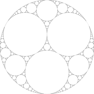
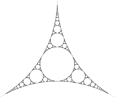
Figure 1. (i) The Standard Apollonian Packing; (ii) The Apollonian Gasket

1.4. Statistical results

A second aim of this monograph is to consider the statistical properties of the distribution of the different weights $\lambda_{\rho}(\omega)$ and $\text{\rm{diam}}(\varphi_{\omega}(X))$ corresponding to words $\omega$ with the same length $n$. In the context of attracting and parabolic GDMSs we have the following Central Limit Theorem, see Part III. We refer the reader to the appropriate section for a detailed definitions of the hypothesis.

Theorem 1.5.

If $\mathcal{S}$ is either a strongly regular finitely irreducible D–generic conformal GDMS or a finite alphabet irreducible parabolic GDMS with $\delta>\frac{2p}{p+1}$ , then there exists $\sigma^{2}>0$ such that if $G\subset\mathbb{R}$ is a Lebesgue measurable set with $\hbox{{\rm Leb}}(\partial G)=0$, then

$$\lim_{n\to+\infty}\mu_{\delta}\left(\left\{\omega\in E_{A}^{\infty}:\frac{-\log\big{|}\varphi_{\omega|_{n}}^{\prime}(\pi_{\mathcal{S}}(\sigma^{n}(\omega)))\big{|}-\chi_{\mu_{\delta}}n}{\sqrt{n}}\in G\right\}\right)=\frac{1}{\sqrt{2\pi}\sigma}\int_{G}e^{-\frac{t^{2}}{2\sigma^{2}}}\,dt.$$

In particular, for any $\alpha<\beta$

$$\lim_{n\to+\infty}\mu_{\delta}\left(\left\{\omega\in E_{A}^{\infty}:\alpha\leq\frac{-\log\big{|}\varphi_{\omega|_{n}}^{\prime}(\pi_{\mathcal{S}}(\sigma^{n}(\omega)))\big{|}-\chi_{\mu_{\delta}}n}{\sqrt{n}}\leq\beta\right\}\right)=\frac{1}{\sqrt{2\pi}\sigma}\int_{\alpha}^{\beta}e^{-\frac{t^{2}}{2\sigma^{2}}}\,dt.$$

The following result is an alternative Central Limit Theorem considering instead the logarithms of the diameters of the images of reference sets.

Theorem 1.6.

Suppose that there $\mathcal{S}$ is either a strongly regular finitely irreducible D–generic conformal GDMS or a finite alphabet irreducible parabolic GDMS with $\delta>\frac{2p}{p+1}$. Let $\sigma^{2}:=\text{{\rm P}}^{\prime\prime}(0)(\neq 0)$. For every $v\in V$ let $Y_{v}\subset X_{v}$ be a set with at least two points. If $G\subset\mathbb{R}$ is a Lebesgue measurable set with $\hbox{\rm Leb}(\partial G)=0$, then

$$\lim_{n\to+\infty}\mu_{\delta}\left(\left\{\omega\in E_{A}^{\infty}:\frac{-\log\hbox{\rm diam}(\varphi_{\omega|_{n}}(Y_{t(\omega_{n})}))-\chi_{\mu_{\delta}}n}{\sqrt{n}}\in G\right\}\right)=\frac{1}{\sqrt{2\pi}\sigma}\int_{G}e^{-\frac{t^{2}}{2\sigma^{2}}}\,dt.$$

In particular, for any $\alpha<\beta$

$$\lim_{n\to+\infty}\mu_{\delta}\left(\left\{\omega\in E_{A}^{\infty}:\alpha\leq\frac{-\log\hbox{\rm diam}(\varphi_{\omega|_{n}}(Y_{t(\omega_{n})}))-\chi_{\mu_{\delta}}n}{\sqrt{n}}\leq\beta\right\}\right)=\frac{1}{\sqrt{2\pi}\sigma}\int_{\alpha}^{\beta}e^{-\frac{t^{2}}{2\sigma^{2}}}\,dt.$$

There are more theorems in this vein proven in Part III, for example the Law of Iterated Logarithm. In order to formulate other statistical results of a slightly different flavor, we define the following measures

$$\mu_{n}(H):=\frac{\sum_{\omega\in H}e^{-\delta\lambda_{\rho}(\omega)}}{\sum_{\omega\in E^{n}_{\rho}}e^{-\delta\lambda_{\rho}(\omega)}}$$

for integers $n\geq 1$ and $H\subset E^{n}_{\rho}$. We also consider the function $\Delta_{n}:E_{A}^{n}\to{\mathbb{R}}$ given by

$$\Delta_{n}(\omega)=\frac{\lambda_{\rho}(\omega)-\chi_{\delta}n}{\sqrt{n}}.$$

Theorem 1.7.

If $\mathcal{S}$ is either a finitely irreducible strongly regular conformal GDMS or a finite alphabet irreducible parabolic GDMS with $\delta>\frac{2p}{p+1}$, then for every $\rho\in E_{A}^{\infty}$ we have that

$$\lim_{n\to+\infty}\int_{E_{\rho}^{n}}\frac{\lambda_{\rho}}{n}d\mu_{n}=\chi_{\mu_{\delta}}=\int_{E_{\rho}^{\infty}}\lambda d\mu_{\delta}.$$

The following theorem describes precisely the magnitude of deviations in this convergence, and is another form of Central Limit Theorem.

Theorem 1.8.

If $\mathcal{S}$ is either a strongly regular finitely irreducible D–generic attracting conformal graph directed Markov system or a finite alphabet irreducible parabolic GDMS with $\delta>\frac{2p}{p+1}$ , then the sequence of random variables $(\Delta_{n})_{n=1}^{\infty}$ converges in distribution to the normal (Gaussian) distribution $\mathcal{N}_{0}(\sigma)$ with mean value zero and the variance $\sigma^{2}=\text{{\rm P}}^{\prime\prime}(\delta)$. Equivalently, the sequence $(\mu_{n}\circ\Delta_{n}^{-1})_{n=1}^{\infty}$ converges weakly to the normal distribution $\mathcal{N}_{0}(\sigma^{2})$. This means that for every Borel set $F\subset\mathbb{R}$ with $\hbox{\rm Leb}(\partial F)=0$, we have

$$\lim_{n\to+\infty}\frac{\sum_{\omega\in E^{n}_{\rho}}\big{|}\varphi_{\omega}^{\prime}(\pi_{\mathcal{S}}(\rho)\big{|}^{\delta}1\!\!\text{{\rm 1}}_{F}\left(\frac{\lambda_{\rho}(\omega|_{n})-\chi_{\delta}n}{\sqrt{n}}\right)}{\sum_{\omega\in E^{n}_{\rho}}\big{|}\varphi_{\omega}^{\prime}(\pi_{\mathcal{S}}(\rho|)\big{|}^{\delta}}=\lim_{n\to+\infty}\mu_{n}(\Delta_{n}^{-1}(F))=\frac{1}{\sqrt{2\pi}\sigma}\int_{F}e^{-t^{2}/2\sigma^{2}}dt.$$

In particular all these theorems hold for all classes of examples described in subsection 1.3, in the case of parabolic systems under the additional hypothesis that $\delta>\frac{2p}{p+1}$, which ensures that the corresponding invariant measure $\mu_{\delta}$ is finite, thus probabilistic after normalization. In the case of continued fractions these take on exactly the same form, in the case of Kleinian groups, including Apollonian circle packings, the same form for associated GDMSs.

However, in giving statements of the Central Limit Theorems for examples we have chosen rational functions to best illustrate them. The first result is a Central Limit Theorem for the distribution of the derivatives of $T$ along orbits.

Theorem 1.9.

Let $f:\widehat{\mathbb{C}}\to\widehat{\mathbb{C}}$ be either an expanding rational function of the Riemann sphere $\widehat{\mathbb{C}}$ or a parabolic rational function of $\widehat{\mathbb{C}}$ with $\delta>\frac{2p}{p+1}$. Then there exists $\sigma^{2}>0$ such that if $G\subset\mathbb{R}$ is a Lebesgue measurable set with $\hbox{{\rm Leb}}(\partial G)=0$, then

$$\lim_{n\to+\infty}\mu_{\delta}\left(\left\{z\in J(f)\hbox{ : }\frac{\log\big{|}(f^{n})^{\prime}(z)\big{|}-\chi_{\mu_{\delta}}n}{\sqrt{n}}\in G\right\}\right)=\frac{1}{\sqrt{2\pi}\sigma}\int_{G}e^{-\frac{t^{2}}{2\sigma^{2}}}\,dt.$$

In particular, for any $\alpha<\beta$

$$\lim_{n\to+\infty}\mu_{\delta}\left(\left\{z\in J(f)\hbox{ : }\alpha\leq\frac{\log\big{|}(f^{n})^{\prime}(z)\big{|}-\chi_{\mu_{\delta}}n}{\sqrt{n}}\leq\beta\right\}\right)=\frac{1}{\sqrt{2\pi}\sigma}\int_{\alpha}^{\beta}e^{-\frac{t^{2}}{2\sigma^{2}}}\,dt.$$

The second result is a Central limit Theorem describing the diameter of the preimages of reference sets.

Theorem 1.10.

Let $f:\widehat{\mathbb{C}}\to\widehat{\mathbb{C}}$ be either an expanding rational function of the Riemann sphere $\widehat{\mathbb{C}}$ or a parabolic rational function of $\widehat{\mathbb{C}}$ with $\delta>\frac{2p}{p+1}$. Then for every $e\in F$ let $Y_{e}\subset R_{e}$ be a set with at least two points. If $G\subset\mathbb{R}$ is a Lebesgue measurable set with $\hbox{\rm Leb}(\partial G)=0$, then

$$\lim_{n\to+\infty}\mu_{\delta}\left(\left\{z\in J(f)\hbox{ : }\frac{-\log\hbox{\rm diam}\big{(}f_{x}^{-n}(Y_{e(z,n)})\big{)}-\chi_{\mu_{\delta}}n}{\sqrt{n}}\in G\right\}\right)=\frac{1}{\sqrt{2\pi}\sigma}\int_{G}e^{-\frac{t^{2}}{2\sigma^{2}}}\,dt$$

where $f_{x}^{-n}$ is a local inverse for $f^{n}$ in a neighbourhood of $x=f^{n}(z)$. In particular, for any $\alpha<\beta$

$$\lim_{n\to+\infty}\mu_{\delta}\left(\left\{z\in J(f)\hbox{ : }\alpha\leq\frac{-\log\hbox{\rm diam}\big{(}f_{x}^{-n}(Y_{e(z,n)})\big{)}-\chi_{\mu_{\delta}}n}{\sqrt{n}}\leq\beta\right\}\right)=\frac{1}{\sqrt{2\pi}\sigma}\int_{\alpha}^{\beta}e^{-\frac{t^{2}}{2\sigma^{2}}}\,dt.$$

Theorem 1.11.

If $f:\widehat{\mathbb{C}}\to\widehat{\mathbb{C}}$ is either an expanding rational function of the Riemann sphere $\widehat{\mathbb{C}}$ or a parabolic rational function of $\widehat{\mathbb{C}}$ with $\delta>\frac{2p}{p+1}$, then for every $\xi\in J(f)$, we have that

$$\lim_{n\to+\infty}\int_{f^{-n}(\xi)}\frac{\log\big{|}(f^{n})^{\prime}\big{|}}{n}d\mu_{n}=\chi_{\delta}.$$

The final result is a Central Limit Theorem which describes the distribution of preimages of a reference point.

Theorem 1.12.

If $f:\widehat{\mathbb{C}}\to\widehat{\mathbb{C}}$ is either an expanding rational function of the Riemann sphere $\widehat{\mathbb{C}}$ or a parabolic rational function of $\widehat{\mathbb{C}}$ with $\delta>\frac{2p}{p+1}$, then the sequence of random variables $(\Delta_{n})_{n=1}^{\infty}$ converges in distribution to the normal (Gaussian) distribution $\mathcal{N}_{0}(\sigma)$ with mean value zero and the variance $\sigma^{2}>0$. Equivalently, the sequence $(\mu_{n}\circ\Delta_{n}^{-1})_{n=1}^{\infty}$ converges weakly to the normal distribution $\mathcal{N}_{0}(\sigma^{2})$. This means that for every Borel set $F\subset\mathbb{R}$ with $\hbox{\rm Leb}(\partial F)=0$, we have

$$\lim_{n\to+\infty}\!\!\frac{\sum_{z\in f^{-n}(\xi)}|(f^{n})^{\prime}(z)|^{-\delta}1\!\!\text{{\rm 1}}_{F}\left(\frac{\log|(f^{n})^{\prime}(z)|-\chi_{\delta}n}{\sqrt{n}}\right)}{\sum_{z\in f^{-n}(\xi)}|(f^{n})^{\prime}(z)|^{-\delta}}=\lim_{n\to+\infty}\mu_{n}(\Delta_{n}^{-1}(F))=\frac{1}{\sqrt{2\pi}\sigma}\int_{F}e^{-t^{2}/2\sigma^{2}}dt.$$

Part I Attracting Conformal Graph Directed Markov Systems

2. Thermodynamic Formalism of Subshifts of Finite Type with Countable Alphabet; Preliminaries

In this section we introduce the basic symbolic setting in which we will be working. We will describe the fundamental thermodynamic concepts, ideas and results, particularly those related to the associated Ruelle-Perron-Frobenius operators, which will play a crucial role throughout the monograph.

Let $\mathbb{N}=\{1,2,\ldots\}$ be the set of all positive integers and let $E$ be a countable set, either finite or infinite, called in the sequel an alphabet. Let

$$\sigma:E^{\mathbb{N}}\to E^{\mathbb{N}}$$

be the shift map, i.e. cutting off the first coordinate and shifting one place to the left. It is given by the formula

$$\sigma\big{(}(\omega_{n})^{\infty}_{n=1}\big{)}=\big{(}(\omega_{n+1})^{\infty}_{n=1}\big{)}.$$

We also set

$$E^{*}=\bigcup_{n=0}^{\infty}E^{n}.$$

to be the set of finite strings. For every $\omega\in E^{*}$, we denote by $|\omega|$ the unique integer $n\geq 0$ such that $\omega\in E^{n}$. We call $|\omega|$ the length of $\omega$. We make the convention that $E^{0}=\{\emptyset\}$. If $\omega\in E^{\mathbb{N}}$ and $n\geq 1$, we put

$$\omega|_{n}=\omega_{1}\ldots\omega_{n}\in E^{n}.$$

If $\tau\in E^{*}$ and $\omega\in E^{*}\cup E^{\mathbb{N}}$, we define the concatenation of $\tau$ and $\omega$ by:

$$\tau\omega:=\begin{cases}\tau_{1}\dots\tau_{|\tau|}\omega_{1}\omega_{2}\dots\omega_{|\omega|}\ \ &{\rm if}\ \omega\in E^{*},\\ \tau_{,}\dots\tau_{|\tau|}\omega_{1}\omega_{2}\dots\ \ &{\rm if}\ \omega\in E^{\mathbb{N}},.\end{cases}$$

Given $\omega,\tau\in E^{\mathbb{N}}$, we define $\omega\wedge\tau\in E^{\mathbb{N}}\cup E^{*}$ to be the longest initial block common to both $\omega$ and $\tau$. For each $\alpha>0$, we define a metric $d_{\alpha}$ on $E^{\mathbb{N}}$ by setting

(2.1) $$d_{\alpha}(\omega,\tau)={\rm e}^{-\alpha|\omega\wedge\tau|}.$$

All these metrics induce the same topology, known to be the product (Tichonov) topology. A real or complex valued function defined on a subset of $E^{\mathbb{N}}$ is uniformly continuous with respect to one of these metrics if and only if it is uniformly continuous with respect to all of them. Also, this function is Hölder with respect to one of these metrics if and only if it is Hölder with respect to all of them although, of course, the Hölder exponent depends on the metric. If no metric is specifically mentioned, we take it to be $d_{1}$.

Now consider an arbitrary matrix $A:E\times E\to\{0,1\}$. Such a matrix will be called the incidence matrix in the sequel. Set

$$E^{\infty}_{A}:=\{\omega\in E^{\mathbb{N}}:\,\,A_{\omega_{i}\omega_{i+1}}=1\,\,\mbox{for all}\,\,i\in{\mathbb{N}}\}.$$

Elements of $E^{\infty}_{A}$ are called $A$-admissible. We also set

$$E^{n}_{A}:=\{\omega\in E^{\mathbb{N}}:\,\,A_{\omega_{i}\omega_{i+1}}=1\,\,\mbox{for all}\,\,1\leq i\leq n-1\},\ n\in{\mathbb{N}},$$

and

$$E^{*}_{A}:=\bigcup_{n=0}^{\infty}E^{n}_{A}.$$

The elements of these sets are also called $A$-admissible. For every $\omega\in E^{*}_{A}$, we put

$$[\omega]:=\{\tau\in E^{\infty}_{A}:\,\,\tau_{|_{|\omega|}}=\omega\}.$$

The set $[\omega]$ is called the cylinder generated by the word $\omega$. The collection of all such cylinders forms a base for the product topology relative to $E^{\infty}_{A}$. The following fact is obvious.

Proposition 2.1.

The set $E^{\infty}_{A}$ is a closed subset of $E^{\mathbb{N}}$, invariant under the shift map $\sigma:E^{\mathbb{N}}\to E^{\mathbb{N}}$, the latter meaning that

$$\sigma(E^{\infty}_{A})\subseteq E^{\infty}_{A}.$$

The matrix $A$ is said to be finitely irreducible if there exists a finite set $\Lambda\subseteq E_{A}^{*}$ such that for all $i,j\in E$ there exists $\omega\in\Lambda$ for which $i\omega j\in E_{A}^{*}$. If all elements of some such $\Lambda$ are of the same length, then $A$ is called finitely primitive (or aperiodic).

The topological pressure of a continuous function $f:E_{A}^{\infty}\to{\mathbb{R}}$ with respect to the shift map $\sigma:E_{A}^{\infty}\to E_{A}^{\infty}$ is defined to be

(2.2) $$\text{{\rm P}}(f):=\lim_{n\to\infty}\frac{1}{n}\log\sum_{\omega\in E_{A}^{n}}\exp\left(\sup_{\tau\in[\omega]}\sum_{j=0}^{n-1}f(\sigma^{j}(\tau))\right).$$

The existence of this limit, following from the observation that the “$\log$” above forms a subadditive sequence, was established in [31], comp. [32]. Following the common usage we abbreviate

$$S_{n}f:=\sum_{j=0}^{n-1}f\circ\sigma^{j}$$

and call $S_{n}f(\tau)$ the $n$th Birkhoff’s sum of $f$ evaluated at a word $\tau\in E_{A}^{\infty}$.

Observe that a function $f:E_{A}^{\infty}\to{\mathbb{R}}$ is (locally) Hölder continuous with an exponent $\alpha>0$ if and only if

$$V_{\alpha}(f):=\sup_{n\geq 1}\{V_{\alpha,n}(f)\}<+\infty,$$

where

$$V_{\alpha,n}(f)=\sup\{|f(\omega)-f(\tau)|e^{\alpha(n-1)}:\omega,\tau\in E_{A}^{\infty}\text{ and }|\omega\wedge\tau|\geq n\}.$$

Observe further that $\text{{\rm H}}_{\alpha}(A)$, the vector space of all bounded Hölder continuous functions $f:E_{A}^{\infty}\to{\mathbb{R}}\,({\rm or\ }{\mathbb{C}})$ with an exponent $\alpha>0$ becomes a Banach space with the norm $||\cdot||_{\alpha}$ defined as follows:

$$||f||_{\alpha}:=||f||_{\infty}+V_{\alpha}(f).$$

The following theorem has been proved in [31], comp. [32], for the class of acceptable functions defined there. Since Hölder continuous ones are among them, we have the following.

Theorem 2.2 (Variational Principle).

If the incidence matrix $A:E\times E\to\{0,1\}$ is finitely irreducible and if $f:E_{A}^{\infty}\to{\mathbb{R}}$ is Hölder continuous, then

$$\text{{\rm P}}(f)=\sup\Big{\{}{\rm h}_{\mu}(\sigma)+\int f\,d\mu\Big{\}},$$

where the supremum is taken over all $\sigma$-invariant (ergodic) Borel probability measures $\mu$ such that $\int f\,d\mu>-\infty$.

We call a $\sigma$-invariant probability measure $\mu$ on $E_{A}^{\infty}$ an equilibrium state of a Hölder continuous function $f:E_{A}^{\infty}\to{\mathbb{R}}$ if $\int-f\,d\mu<+\infty$ and

(2.3) $${\rm h}_{\mu}(\sigma)+\int\!\!f\,d\mu=\text{{\rm P}}(f).$$

If $f:E_{A}^{\infty}\to{\mathbb{R}}$ is a Hölder continuous function, then following [31], and [32] a Borel probability measure $\mu$ on $E_{A}^{\infty}$ is called a Gibbs state for $f$ (comp. also [4], [19], [50], [51], [60] and [59]) if there exist constants $Q\geq 1$ and $\text{{\rm P}}_{\mu}\in{\mathbb{R}}$ such that for every $\omega\in E_{A}^{*}$ and every $\tau\in[\omega]$

(2.4) $$Q^{-1}\leq{\mu([\omega])\over\exp\big{(}S_{|\omega|}f(\tau)-\text{{\rm P}}_{\mu}|\omega|\big{)}}\leq Q.$$

If additionally $\mu$ is shift-invariant, it is then called an invariant Gibbs state. It is readily seen from this definition that if a Hölder continuous function $f:E_{A}^{\infty}\to{\mathbb{R}}$ admits a Gibbs state $\mu$, then

$$\text{{\rm P}}_{\mu}=\text{{\rm P}}(f).$$

From now on throughout this section $f:E_{A}^{\infty}\to{\mathbb{R}}$ is assumed to be a Hölder continuous function with an exponent $\alpha>0$, and it is also assumed to satisfy the following requirement

(2.5) $$\sum_{e\in E}\exp(\sup(f|_{[e]}))<+\infty.$$

Functions $f$ satisfying this condition are called (see [31], and [32]) in the sequel summable. We note that if $f$ has a Gibbs state, then $f$ is summable. This requirement of summability, allows us to define the Perron-Frobenius operator

$${\mathcal{L}}_{f}:C_{b}(E_{A}^{\infty})\to C_{b}(E_{A}^{\infty}),$$

acting on the space of bounded continuous functions $C_{b}(E_{A}^{\infty})$ endowed with $\|\cdot\|_{\infty}$, the supremum norm, as follows:

$${\mathcal{L}}_{f}(g)(\omega):=\sum_{e\in E:A_{e\omega_{1}}=1}\exp(f(e\omega)g(e\omega).$$

Then $\|{\mathcal{L}}_{f}\|_{\infty}\leq\sum_{e\in E}\exp(\sup(f|_{[e]}))<+\infty$ and for every $n\geq 1$

$${\mathcal{L}}_{f}^{n}(g)(\omega)=\sum_{\tau\in E_{A}^{n}:A_{\tau_{n}\omega_{1}}=1}\exp\big{(}S_{n}f(\tau\omega)\big{)}g(\tau\omega).$$

The conjugate operator ${\mathcal{L}}_{f}^{*}$ acting on the space $C_{b}^{*}(E_{A}^{\infty})$ has the following form:

$${\mathcal{L}}_{f}^{*}(\mu)(g):=\mu({\mathcal{L}}_{f}(g))=\int{\mathcal{L}}_{f}(g)\,d\mu.$$

Observe that the operator ${\mathcal{L}}_{f}$ preserves the space $\text{{\rm H}}_{\alpha}(A)$, of all Hölder continuous functions with an exponent $\alpha>0$. More precisely

$${\mathcal{L}}_{f}(\text{{\rm H}}_{\alpha}(A))\subseteq\text{{\rm H}}_{\alpha}(A).$$

We now provide a brief account of those elements of the spectral theory that we will need and use in the sequel. Let $B$ be a Banach space and let $L:B\to B$ be a bounded linear operator. A point $\lambda\in{\mathbb{C}}$ is said to belong to the spectral set (spectrum) of the operator $L$ if the operator $\lambda I_{B}-L:B\to B$ is not invertible, where $I_{B}:B\to B$ is the identity operator on $B$. The spectral radius $r(L)$ of $L$ is defined to be the supremum of moduli of all elements in the spectral set of $L$. It is known that $r(L)$ is finite and

$$r(L)=\lim_{n\to\infty}\|L^{n}\|^{1/n}.$$

A point $\lambda$ of the spectrum of $L$ is said to belong to the essential spectral set (essential spectrum) of the operator $L$ if $\lambda$ is not an isolated eigenvalue of $L$ of finite multiplicity. The essential spectral radius $r_{\rm ess}(L)$ of $L$ is defined to be the supremum of moduli of all elements in the essential spectral set of $L$. It is known (see [36]) that

$$r_{\rm ess}(L)=\varlimsup_{n\to\infty}\inf\big{\{}\|L^{n}-K\|^{1/n}\big{\}},$$

where for every $n\geq 1$ the infimum is taken over all compact operators $K:B\to B$. The operator $L:B\to B$ is called quasi-compact if either $r(L)=0$ or

$$r_{\rm ess}(L)<r(L).$$

The proof of the following theorem can be found in [32]. For the items (a)–(f) see also Corollary 4.3.8 in [7].

Theorem 2.3.

Suppose that $f:E_{A}^{\infty}\to{\mathbb{R}}$ is a Hölder continuous summable function and the incidence matrix $A$ is finitely irreducible. Then

• There exists a unique Borel probability eigenmeasure $m_{f}$ of the conjugate Perron-Frobenius operator ${\mathcal{L}}_{f}^{*}$ and the corresponding eigenvalue is equal to $e^{\text{{\rm P}}(f)}$.

• The eigenmeasure $m_{f}$ is a Gibbs state for $f$.

• The function $f:E_{A}^{\infty}\to{\mathbb{R}}$ has a unique $\sigma$-invariant Gibbs state $\mu_{f}$.

• The measure $\mu_{f}$ is ergodic, equivalent to $m_{f}$ and if $\psi_{f}=d\mu_{f}/dm_{f}$ is the Radon–Nikodym derivative of $\mu_{f}$ with respect to $m_{f}$, then $\log\psi_{f}$ is uniformly bounded.

• If $\int-f\,d\mu_{f}<+\infty$, then the $\sigma$-invariant Gibbs state $\mu_{f}$ is the unique equilibrium state for the potential $f$.

• In case the incidence matrix $A$ is finitely primitive, the Gibbs state $\mu_{f}$ is completely ergodic.

• The spectral radius of the operator ${\mathcal{L}}_{f}$ considered as acting either on $C_{b}(E_{A}^{\infty})$ or $\text{{\rm H}}_{\alpha}(A)$ is in both cases equal to $e^{\text{{\rm P}}(f)}$.

• In either case of (g) the number $e^{\text{{\rm P}}(f)}$ is a simple (isolated in the case of $\text{{\rm H}}_{\alpha}(A)$) eigenvalue of ${\mathcal{L}}_{f}$ and the Radon–Nikodym derivative $\psi_{f}\in\text{{\rm H}}_{\alpha}(A)$ generates its eigenspace.

• The remainder of the spectrum of the operator ${\mathcal{L}}_{f}:\text{{\rm H}}_{\alpha}(A)\to\text{{\rm H}}_{\alpha}(A)$ is contained in a union of finitely many eigenvalues of finite multiplicity (different from $e^{\text{{\rm P}}(f)}$) of modulus $e^{\text{{\rm P}}(f)}$ and a closed disk centered at $0$ with radius strictly smaller than $e^{\text{{\rm P}}(f)}$.
  In particular, the operator ${\mathcal{L}}_{f}:\text{{\rm H}}_{\alpha}(A)\to\text{{\rm H}}_{\alpha}(A)$ is quasi-compact.

  In the case where the incidence matrix $A$ is finitely primitive a stronger statement holds: namely, apart from $e^{\text{{\rm P}}(f)}$, the spectrum of ${\mathcal{L}}_{f}:\text{{\rm H}}_{\alpha}(A)\to\text{{\rm H}}_{\alpha}(A)$ is contained in a closed disk centered at $0$ with radius strictly smaller than $e^{\text{{\rm P}}(f)}$.
  In particular, the operator ${\mathcal{L}}_{f}:\text{{\rm H}}_{\alpha}(A)\to\text{{\rm H}}_{\alpha}(A)$ is quasi-compact.

3. Attracting Conformal Countable Alphabet Graph Directed Markov Systems (GDMSs)
and
Countable Alphabet Attracting Iterated Function Systems (IFSs);
Preliminaries

In this article we consider a slightly more general setting than just the usual conformal iterated function systems, namely the ones better suited to modeling the examples in which we are interested. In later sections we will prove the results in this context and explain how they can be used to derive different geometric and dynamical results, such as those already mention in the introduction.

Let us define a graph directed Markov system (abbr. GDMS) relative to a directed multigraph $(V,E,i,t)$ and an incidence matrix $A:E\times E\to\{0,1\}$. Such systems are defined and studied at length in [27] and [32]. A directed multigraph consists of a finite set $V$ of vertices, a countable (either finite or infinite) set $E$ of directed edges, two functions

$$i,t:E\to V,$$

and an incidence matrix $A:E\times E\to\{0,1\}$ on $(V,E,i,t)$ such that

$$A_{ab}=1\ \ \ {\rm implies}\ \ \ t(b)=i(a).$$

Now suppose that in addition, we have a collection of nonempty compact metric spaces $\{X_{v}\}_{v\in V}$ and a number $\kappa\in(0,1)$, such that for every $e\in E$, we have a one-to-one contraction $\varphi_{e}:X_{t(e)}\to X_{i(e)}$ with Lipschitz constant (bounded above by) $\kappa$. Then the collection

$$\mathcal{S}=\{\varphi_{e}:X_{t(e)}\to X_{i(e)}\}_{e\in E}$$

is called an attracting graph directed Markov system (or GDMS). We will frequently refer to it just as a graph directed Markov system or GDMS. We will however always keep the adjective ”parabolic” when, in later sections, we will also speak about parabolic graph directed Markov systems. We extend the functions $i,t:E\to V$ in a natural way to $E_{A}^{*}$ as follows:

$$t(\omega):=t\big{(}\omega_{|\omega|}\big{)}\ \ \ {\rm and}\ \ \ i(\omega):=i(\omega_{1}).$$

For every word $\omega\in E_{A}^{*}$, say $\omega\in E_{A}^{n}$, $n\geq 0$, let us denote

$$\varphi_{\omega}:=\varphi_{\omega_{1}}\circ\cdots\circ\varphi_{\omega_{n}}:X_{t(\omega)}\to X_{i(\omega)}.$$

We now describe the limit set, also frequently called the attractor, of the system $\mathcal{S}$. For any $\omega\in E^{\infty}_{A}$, the sets $\{\varphi_{\omega|_{n}}\left(X_{t(\omega_{n})}\right)\}_{n\geq 1}$ form a descending sequence of nonempty compact sets and therefore $\bigcap_{n\geq 1}\varphi_{\omega|_{n}}\left(X_{t(\omega_{n})}\right)\neq\emptyset$. Since for every $n\geq 1$,

$$\text{\rm{diam}}\left(\varphi_{\omega|_{n}}\left(X_{t(\omega_{n})}\right)\right)\leq\kappa^{n}\text{\rm{diam}}\left(X_{t(\omega_{n})}\right)\leq\kappa^{n}\max\{\text{\rm{diam}}(X_{v}):v\in V\},$$

we conclude that the intersection

$$\bigcap_{n\in{\mathbb{N}}}\varphi_{\omega|_{n}}\left(X_{t(\omega_{n})}\right)$$

is a singleton and we denote its only element by $\pi_{\mathcal{S}}(\omega)$ or simpler, by $\pi(\omega)$. In this way we have defined a map

$$\pi_{\mathcal{S}}=\pi:E^{\infty}_{A}\to X:=\coprod_{v\in V}X_{v},$$

where $\coprod_{v\in V}X_{v}$ is the disjoint union of the compact topological spaces $X_{v}$, $v\in V$. The map $\pi$ is called the coding map, and the set

$$J=J_{\mathcal{S}}=\pi(E^{\infty}_{A})$$

is called the limit set of the GDMS $\mathcal{S}$. The sets

$$J_{v}=\pi(\{\omega\in E_{A}^{\infty}:i(\omega_{1})=v\}),\;\;v\in V,$$

are called the local limit sets of $\mathcal{S}$.

We call the GDMS $\mathcal{S}$ finite if the alphabet $E$ is finite. Furthermore, we call $\mathcal{S}$ maximal if for all $a,b\in E$, we have $A_{ab}=1$ if and only if $t(b)=i(a)$. In [32], a maximal GDMS was called a graph directed system (abbr. GDS). Finally, we call a maximal GDMS $\mathcal{S}$ an iterated function system (or IFS) if $V$, the set of vertices of $\mathcal{S}$, is a singleton. Equivalently, a GDMS is an IFS if and only if the set of vertices of $\mathcal{S}$ is a singleton and all entries of the incidence matrix $A$ are equal to $1$.

Definition 3.1.

We call the GDMS $\mathcal{S}$ and its incidence matrix $A$ finitely irreducible if there exists a finite set $\Omega\subset E_{A}^{*}$ such that for all $a,b\in E$ there exists a word $\omega\in\Omega$ such that the concatenation $a\omega b$ is in $E_{A}^{*}$. $\mathcal{S}$ and $A$ are called finitely primitive if the set $\Omega$ may be chosen to consist of words all having the same length. If such a set $\Omega$ exists but is not necessarily finite, then $\mathcal{S}$ and $A$ are called irreducible and primitive, respectively. Note that all IFSs are symbolically irreducible.

Remark 3.2.

For every integer $q\geq 1$ define $\mathcal{S}^{q}$, the $q$th iterate of the system $\mathcal{S}$, to be

$$\{\varphi_{\omega}:X_{t(\omega)}\to X_{i(\omega)}:\omega\in E_{A}^{q}\}$$

and its alphabet is $E_{A}^{q}$. All the theorems proved in this monograph hold under the formally weaker hypothesis that all the elements of some iterate $\mathcal{S}^{q}$, $q\geq 1$, of the system $\mathcal{S}$, are uniform contractions. This in particular pertains to the Gauss system of Example 17.14 for which $q=2$ works.

With the aim of moving on to geometric applications, and following [32], we call a GDMS conformal if for some $d\in{\mathbb{N}}$, the following conditions are satisfied.

• For every vertex $v\in V$, $X_{v}$ is a compact connected subset of ${\mathbb{R}}^{d}$, and $X_{v}=\overline{\text{{\rm Int}}(X_{v})}$.

• (Open Set Condition) For all $a,b\in E$ such that $a\neq b$,

  $$\varphi_{a}(\text{{\rm Int}}(X_{t(a)}))\cap\varphi_{b}(\text{{\rm Int}}(X_{t(b)}))=\emptyset.$$

• (Conformality) There exists a family of open connected sets $W_{v}\subset X_{v}$, $v\in V$, such that for every $e\in E$, the map $\varphi_{e}$ extends to a $C^{1}$ conformal diffeomorphism from $W_{t(e)}$ into $W_{i(e)}$ with Lipschitz constant $\leq\kappa$.

• (Bounded Distortion Property (BDP)) There are two constants $L\geq 1$ and $\alpha>0$ such that for every $e\in E$ and every pair of points $x,y\in X_{t(e)}$,

  $$\bigg{|}\frac{|\varphi_{e}^{\prime}(y)|}{|\varphi_{e}^{\prime}(x)|}-1\bigg{|}\leq L\|y-x\|^{\alpha},$$

  where $|\varphi_{\omega}^{\prime}(x)|$ denotes the scaling factor of the derivative $\varphi_{\omega}^{\prime}(x):{\mathbb{R}}^{d}\to{\mathbb{R}}^{d}$ which is a similarity map.

Remark 3.3.

When $d=1$ the conformality is automatic. If $d\geq 2$ and a family $\mathcal{S}=\{\varphi_{e}\}_{e\in E}$ satisfies the conditions (a) and (c), then it also satisfies condition (d) with $\alpha=1$. When $d=2$ this is due to the well-known Koebe’s Distortion Theorem (see for example, [8, Theorem 7.16], [8, Theorem 7.9], or [21, Theorem 7.4.6]). When $d\geq 3$ it is due to [32] depending heavily on Liouville’s representation theorem for conformal mappings; see [23] for a detailed development of this theorem leading up to the strongest current version, and also including exhaustive references to the historical background.

For every real number $s\geq 0$, let (see [27] and [32])

$$\text{{\rm P}}(s):=\lim_{n\to+\infty}\frac{1}{n}\log\left(\sum_{|\omega|=n}\|\varphi_{\omega}^{\prime}\|_{\infty}^{s}\right),$$

where $\|\varphi^{\prime}\|_{\infty}$ denotes the supremum norm of the derivative of a conformal map $\varphi$ over its domain; in our context these domains will be always the sets $X_{v}$, $v\in V$. The above limit always exists because the corresponding sequence is clearly subadditive. The number $\text{{\rm P}}(s)$ is called the topological pressure of the parameter $s$. Because of the Bounded Distortion Property (i.e., Property (d)), we have also the following characterization of topological pressure:

$$\text{{\rm P}}(s):=\lim_{n\to+\infty}\frac{1}{n}\log\left(\sum_{|\omega|=n}|\varphi_{\omega}^{\prime}(z_{\omega})|^{s}\right),$$

where $\{z_{\omega}:\omega\in E_{A}^{*}\}$ is an entirely arbitrary set of points such that $z_{\omega}\in X_{t(\omega)}$ for every $\omega\in E_{A}^{*}$. Let $\zeta:E^{\infty}_{A}\to\mathbb{R}$ be defined by the formula

(3.1) $$\zeta(\omega):=\log|\varphi^{\prime}_{\omega_{1}}(\pi(\sigma(\omega))|.$$

The following proposition is easy to prove; see [32, Proposition 3.1.4] for complete details.

Proposition 3.4.

For every real $s\geq 0$ the function $s\zeta:E^{\infty}_{A}\to\mathbb{R}$ is Hölder continuous and

$$\text{{\rm P}}(s\zeta)=\text{{\rm P}}(s).$$

Definition 3.5.

We say that a nonnegative real number $s$ belongs to $\Gamma_{\mathcal{S}}$ if

(3.2) $$\sum_{e\in E}\|\varphi^{\prime}_{e}\|_{\infty}^{s}<+\infty.$$

Let us record the following immediate observation.

Observation 3.6.

A nonnegative real number $s$ belongs to $\Gamma_{\mathcal{S}}$ if and only if the Hölder continuous potential $s\zeta:E_{A}^{\infty}\to{\mathbb{R}}$ is summable.

We recall from [27] and [32] the following definitions:

$$\gamma_{\mathcal{S}}:=\inf\Gamma_{\mathcal{S}}=\inf\left\{s\geq 0:\sum_{e\in E}\|\varphi_{e}^{\prime}\|_{\infty}^{s}<+\infty\right\}.$$

The proofs of the following two statements can be found in [32].

Proposition 3.7.

If $\mathcal{S}$ is an irreducible conformal GDMS, then for every $s\geq 0$ we have that

$$\Gamma_{\mathcal{S}}=\{s\geq 0:\text{{\rm P}}(s)<+\infty\}$$

In particular,

$$\gamma_{\mathcal{S}}:=\inf\left\{s\geq 0:\text{{\rm P}}(s)<+\infty\right\}.$$

Theorem 3.8.

If $\mathcal{S}$ is a finitely irreducible conformal GDMS, then the function $\Gamma_{\mathcal{S}}\ni s\mapsto\text{{\rm P}}(s)\in{\mathbb{R}}$ is

1. strictly decreasing,

2. real-analytic,

3. convex, and

4. $\lim_{s\to+\infty}\text{{\rm P}}(s)=-\infty$.

We denote

$${\mathcal{L}}_{s}:={\mathcal{L}}_{s\zeta}$$

acting either on $C_{b}(E_{A}^{\infty})$ or on $\text{{\rm H}}_{a}(A)$. Because of Proposition 3.4 and Observation 3.6, our Theorem 2.3 applies to all functions $s\zeta:E_{A}^{\infty}\to{\mathbb{R}}$ giving the following.

Theorem 3.9.

Suppose that the system $\mathcal{S}$ is finitely irreducible and $s\in\Gamma_{\mathcal{S}}$. Then

• There exists a unique Borel probability eigenmeasure $m_{s}$ of the conjugate Perron-Frobenius operator ${\mathcal{L}}_{s}^{*}$ and the corresponding eigenvalue is equal to $e^{\text{{\rm P}}(s)}$.

• The eigenmeasure $m_{s}$ is a Gibbs state for $t\zeta$.

• The function $s\zeta:E_{A}^{\infty}\to{\mathbb{R}}$ has a unique $\sigma$-invariant Gibbs state $\mu_{s}$.

• The measure $\mu_{s}$ is ergodic, equivalent to $m_{s}$ and if $\psi_{s}=d\mu_{s}/dm_{s}$ is the Radon–Nikodym derivative of $\mu_{s}$ with respect to $m_{s}$, then $\log\psi_{s}$ is uniformly bounded.

• If $\chi_{\mu_{s}}:=-\int\zeta\,d\mu_{s}<+\infty$, then the $\sigma$-invariant Gibbs state $\mu_{s}$ is the unique equilibrium state for the potential $s\zeta$.

• In case the the system $\mathcal{S}$ is finitely primitive, the Gibbs state $\mu_{s}$ is completely ergodic.

• The spectral radius of the operator ${\mathcal{L}}_{s}$ considered as acting either on $C_{b}(E_{A}^{\infty})$ or $\text{{\rm H}}_{\alpha}(A)$ is in both cases equal to $e^{\text{{\rm P}}(s)}$.

• In either case of (g) the number $e^{\text{{\rm P}}(s)}$ is a simple (isolated in the case of $\text{{\rm H}}_{\alpha}(A)$) eigenvalue of ${\mathcal{L}}_{s}$ and the Radon–Nikodym derivative $\psi_{s}\in\text{{\rm H}}_{\alpha}(A)$ generates its eigenspace.

• The reminder of the spectrum of the operator ${\mathcal{L}}_{s}:\text{{\rm H}}_{\alpha}(A)\to\text{{\rm H}}_{\alpha}(A)$ is contained in a union of finitely many eigenvalues (different from $e^{\text{{\rm P}}(s)}$) of modulus $e^{\text{{\rm P}}(s)}$ and a closed disk centered at $0$ with radius strictly smaller than $e^{\text{{\rm P}}(s)}$ (if $A$ is finitely primitive, then these eigenvalues of modulus smaller than $e^{\text{{\rm P}}(s)}$ disappear). In particular, the operator ${\mathcal{L}}_{s}:\text{{\rm H}}_{\alpha}(A)\to\text{{\rm H}}_{\alpha}(A)$ is quasi-compact.

Given $s\in\Gamma_{\mathcal{S}}$ it immediately follows from this theorem and the definition of Gibbs states that

(3.3) $$C_{s}^{-1}e^{-\text{{\rm P}}(s)|\omega|}\|\varphi_{\omega}^{\prime}\|_{\infty}^{s}\leq m_{s}([\omega])\asymp\mu_{s}([\omega])\leq C_{s}e^{-\text{{\rm P}}(s)|\omega|}\|\varphi_{\omega}^{\prime}\|_{\infty}^{s}$$

for all $\omega\in E_{A}^{*}$, where $C_{s}\geq 1$ denotes some constant. We put

(3.4) $$\widetilde{m}_{s}:=m_{s}\circ\pi_{\mathcal{S}}^{-1}\ \ \ {\rm and}\ \ \ \widetilde{\mu}_{s}:=\mu_{s}\circ\pi_{\mathcal{S}}^{-1}.$$

The measure $\widetilde{m}_{s}$ is characterized (see [32]) by the following two properties:

(3.5) $$\widetilde{m}_{s}(\varphi_{e}(F))=e^{-\text{{\rm P}}(s)}\int_{F}|\varphi_{e}^{\prime}|\,d\widetilde{m}_{s}$$

for every $e\in E$ and every Borel set $F\subseteq X_{t(e)}$, and

(3.6) $$\widetilde{m}_{s}\big{(}\varphi_{a}(X_{t(a)})\cap\varphi_{b}(X_{t(b)})\big{)}=0$$

whenever $a,b\in E$ and $a\neq b$. By a straightforward induction these extend to

(3.7) $$\widetilde{m}_{s}(\varphi_{\omega}(F))=e^{-\text{{\rm P}}(s)|\omega|}\int_{F}|\varphi_{\omega}^{\prime}|\,d\widetilde{m}_{s}$$

for every $\omega\in E_{A}^{*}$ and every Borel set $F\subseteq X_{t(\omega)}$, and

(3.8) $$\widetilde{m}_{s}\big{(}\varphi_{\alpha}(X_{t(\alpha)})\cap\varphi_{\beta}(X_{t(\beta)})\big{)}=0$$

whenever $\alpha,\beta\in E_{A}^{*}$ and are incomparable.

The following theorem, providing a geometrical interpretation of the parameter $\delta_{\mathcal{S}}$, has been proved in [32] ([27] in the case of IFSs).

Theorem 3.10.

If $\mathcal{S}$ is an finitely irreducible conformal GDMS, then

$$\delta=\delta_{\mathcal{S}}:=\text{{\rm HD}}(J_{\mathcal{S}})=\inf\{s\geq 0:\text{{\rm P}}(s)\leq 0\}\geq\gamma_{\mathcal{S}}.$$

Following [27] and [32] we call the system $\mathcal{S}$ regular if there exists $s\in(0,+\infty)$ such that

$$\text{{\rm P}}(s)=0.$$

Then by Theorems 3.10 and 3.8, such zero is unique and is equal to $\delta_{\mathcal{S}}$. So,

(3.9) $$\text{{\rm P}}(\delta_{\mathcal{S}})=0.$$

Formula (3.3) then takes the following form:

(3.10) $$C_{\delta_{\mathcal{S}}}^{-1}\|\varphi_{\omega}^{\prime}\|_{\infty}^{\delta_{\mathcal{S}}}\leq m_{\delta_{\mathcal{S}}}([\omega])\asymp\mu_{\delta_{\mathcal{S}}}([\omega])\leq C_{\delta_{\mathcal{S}}}\|\varphi_{\omega}^{\prime}\|_{\infty}^{\delta_{\mathcal{S}}}$$

for all $\omega\in E_{A}^{*}$. The measure $\widetilde{m}_{\delta_{\mathcal{S}}}$ is then referred to as the $\delta_{\mathcal{S}}$–conformal measure of the system $\mathcal{S}$.

Also following [27] and [32], we call the system $\mathcal{S}$ strongly regular if there exists $s\in[0,+\infty)$ (in fact in $(\gamma_{\mathcal{S}},+\infty)$) such that

$$0<\text{{\rm P}}(s)<+\infty.$$

Because of Theorem 3.8 each strongly regular conformal GDMS is regular. Furthermore, we record the following two immediate observations.

Observation 3.11.

If $s\in\text{{\rm Int}}(\Gamma_{\mathcal{S}})$, then $\chi_{\mu_{s}}<+\infty$.

Observation 3.12.

A finitely irreducible conformal GDMS $\mathcal{S}$ is strongly regular if and only if

$$\gamma_{\mathcal{S}}<\delta_{\mathcal{S}}.$$

In particular, if the system $\mathcal{S}$ is a strongly regular, then $\delta_{\mathcal{S}}\in\text{{\rm Int}}(\Gamma_{\mathcal{S}})$.

These two observations yield the following.

Corollary 3.13.

If a finitely irreducible conformal GDMS $\mathcal{S}$ is strongly regular, then $\chi_{\mu_{\delta}}<+\infty$.

We will also need the following fact, well-known in the case of finite alphabets $E$, and proved for all countable alphabets in [32].

Theorem 3.14.

If $s\in\text{{\rm Int}}(\Gamma_{\mathcal{S}})$, then

$$\text{{\rm P}}^{\prime}(s)=-\chi_{\mu_{s}}.$$

In particular this formula holds if the system $\mathcal{S}$ is strongly regular and $s=\delta_{\mathcal{S}}$.

We end this section by noting that each finite irreducible system is strongly regular.

4. Complex Ruelle–Perron–Frobenius Operators; Spectrum and D–Genericity

A key ingredient when analyzing the Poincaré series $\eta_{\xi}(s)$ and $\eta_{p}(s)$ mentioned in the introduction is to use complex Ruelle-Perron-Frobenius or Transfer operators. These are closely related to the RPF operators already introduced, except that we now allow the weighting function to take complex values. More precisely, we extend the definition of operators ${\mathcal{L}}_{s}$, $s\in\Gamma_{\mathcal{S}}$, to the complex half-plane

$$\Gamma_{\mathcal{S}}^{+}:=\{s\in{\mathbb{C}}:\text{{\rm Re}}s>\gamma_{\mathcal{S}}\},$$

in a most natural way; namely, for every $s\in\Gamma_{\mathcal{S}}^{+}$, we set

(4.1) $${\mathcal{L}}_{s}(g)(\omega)=\sum_{e\in E:A_{e\omega_{1}}=1}|\varphi_{e}^{\prime}(\pi(\omega))|^{s}g(e\omega).$$

Clearly these linear operators ${\mathcal{L}}_{s}$ act on both Banach spaces $C_{b}(E_{A}^{\infty})$ and $\text{{\rm H}}_{a}(A)$, are bounded, and we have the following.

Observation 4.1.

The function

$$\Gamma_{\mathcal{S}}^{+}\ni s\mapsto{\mathcal{L}}_{s}\in L(\text{{\rm H}}_{a}(A))$$

is holomorphic, where $L(\text{{\rm H}}_{a}(A))$ is the Banach space of all bounded linear operators on $\text{{\rm H}}_{a}(A)$ endowed with the operator norm.

Proposition 4.2.

Let $\mathcal{S}$ be a finitely irreducible conformal GDMS. Then for every $s=\sigma+it\in\Gamma_{\mathcal{S}}^{+}$

1. the spectral radius $r({\mathcal{L}}_{s})$ of the operator ${\mathcal{L}}_{s}:\text{{\rm H}}_{\alpha}(A)\to\text{{\rm H}}_{a}(A)$ is not larger than $e^{\text{{\rm P}}(\sigma)}$ and

2. the essential spectral radius $r_{\rm ess}({\mathcal{L}}_{s})$ of the operator ${\mathcal{L}}_{s}:\text{{\rm H}}_{\alpha}(A)\to\text{{\rm H}}_{a}(A)$ is not larger than $e^{-\alpha}e^{\text{{\rm P}}(\sigma)}$.

Proof.

Assume without loss of generality that $E={\mathbb{N}}$. For every $\omega\in E_{A}^{*}$ choose arbitrarily $\hat{\omega}\in[\omega]$. Now for every integer $n\geq 1$ define the linear operator

$$E_{n}:\text{{\rm H}}_{\alpha}(A)\to\text{{\rm H}}_{a}(A)$$

by the formula

(4.2) $$E_{n}(g):=\sum_{\omega\in E_{A}^{n}}g(\hat{\omega})1\!\!\text{{\rm 1}}_{[\omega]}.$$

Equivalently

$$E_{n}(g)=g(\hat{\omega}),\ \omega\in E_{A}^{\infty}.$$

Of course $||E_{n}(g)||_{\alpha}\leq||g||_{\alpha}$ and $E_{n}$ is a bounded operator with $||E_{n}||_{\alpha}\leq 1$. However, the series (4.2) is not uniformly convergent, i.e. it is not convergent in the supremum norm $||\cdot||_{\infty}$, thus not in the Hölder norm $||\cdot||_{\alpha}$ either. For all integers $N\geq 1$ and $n\geq 1$ denote

$$E_{A}^{n}(N):=\{\omega\in E_{A}^{n}:\forall_{j\leq n}\,\omega_{j}\leq N\}$$

and

$$E_{A}^{n}(N+):=\{\omega\in E_{A}^{n}:\exists_{j\leq n}\,\omega_{j}>N\}.$$

Let us further write

$$E_{n,N}g:=\sum_{\omega\in E_{A}^{n}(N)}g(\hat{\omega})1\!\!\text{{\rm 1}}_{[\omega]}$$

and

$$E_{n,N}^{+}g:=\sum_{\omega\in E_{A}^{n}(N+)}g(\hat{\omega})1\!\!\text{{\rm 1}}_{[\omega]}.$$

Of course $E_{n,N}:\text{{\rm H}}_{\alpha}(A)\to\text{{\rm H}}_{a}(A)$ is a finite–rank operator, thus compact. Therefore, the composite operator ${\mathcal{L}}_{s}E_{n,N}:\text{{\rm H}}_{\alpha}(A)\to\text{{\rm H}}_{a}(A)$ is also compact. We know that

(4.3) $$\|{\mathcal{L}}_{s}^{n}-{\mathcal{L}}_{s}^{n}E_{n,N}\|_{\alpha} =\|({\mathcal{L}}_{s}^{n}-{\mathcal{L}}_{s}^{n}E_{n})+{\mathcal{L}}_{s}^{n}(E_{n}-E_{n,N})\|_{\alpha}=\|{\mathcal{L}}_{s}^{n}(I-E_{n})+{\mathcal{L}}_{s}^{n}E_{n,N}^{+}\|_{\alpha}$$

$$\leq\|{\mathcal{L}}_{s}^{n}(I-E_{n})\|_{\alpha}+\|{\mathcal{L}}_{s}^{n}E_{n,N}^{+}\|_{\alpha}.$$

We will estimate from above each of the last two terms separately. We begin first with the first of these two terms. In the same way as for real parameters $s$, which is done in [32], one proves for all operators ${\mathcal{L}}_{s}:\text{{\rm H}}_{\alpha}(A)\to\text{{\rm H}}_{a}(A)$ the following form of the Ionescu–Tulcea–Marinescu inequality:

(4.4) $$\|{\mathcal{L}}_{s}^{n}g\|_{\alpha}\leq Ce^{\text{{\rm P}}(\sigma)n}\big{(}\|g\|_{\infty}+e^{-\alpha n}\|g\|_{\alpha}\big{)}$$

with some constant $C>0$. This establishes item (1) of our theorem. Since a straightforward calculation shows that $\|g-E_{n}g\|_{\alpha}\leq 2\|g\|_{\alpha}$ and $\|g-E_{n}g\|_{\infty}\leq\|g|_{\alpha}e^{-\alpha n}$ , we therefore get that

$$\|{\mathcal{L}}_{s}^{n}(I-E_{n})g\|_{\alpha}\leq Ce^{\text{{\rm P}}(\sigma)n}\big{(}\|g\|_{\alpha}e^{-\alpha n}+2e^{-\alpha n}\|g\|_{\alpha}\big{)}=3Ce^{\text{{\rm P}}(\sigma)n}e^{-\alpha n}\|g\|_{\alpha}.$$

Thus,

(4.5) $$||{\mathcal{L}}_{s}^{n}(I-E_{n})||_{\alpha}\leq 3Ce^{\text{{\rm P}}(\sigma)n}e^{-\alpha n}.$$

Passing to the estimate of the second term, we have

$${\mathcal{L}}_{s}^{n}E_{n,N}^{+}g(\omega)=\sum_{{\tau\in E_{A}^{n}(N+)\atop\tau\omega\in E_{A}^{\infty}}}g(\hat{\tau})|\varphi_{\tau}^{\prime}(\pi(\sigma(\omega)))|^{s}.$$

Therefore,

$$\|{\mathcal{L}}_{s}^{n}E_{n,N}^{+}g\|_{\alpha} \leq\sum_{\tau\in E_{A}^{n}(N+)}|g(\hat{\tau})|\Big{\|}\big{|}\varphi_{\tau}^{\prime}\circ\pi\circ\sigma\big{|}^{s}\Big{\|}_{\alpha}$$

$$\leq\|g\|_{\infty}\sum_{\tau\in E_{A}^{n}(N+)}\Big{\|}\big{|}\varphi_{\tau}^{\prime}\circ\pi\circ\sigma\big{|}^{s}\Big{\|}_{\alpha}$$

$$\leq\|g\|_{\infty}\sum_{\tau\in E_{A}^{n}(N+)}\Big{\|}\big{|}\varphi_{\tau}^{\prime}\circ\pi\circ\sigma\big{|}^{s}\Big{\|}_{\alpha}.$$

Hence,

(4.6) $$\|{\mathcal{L}}_{s}^{n}E_{n,N}^{+}\|_{\alpha}\leq\sum_{\tau\in E_{A}^{n}(N+)}\Big{\|}\big{|}\varphi_{\tau}^{\prime}\circ\pi\circ\sigma\big{|}^{s}\Big{\|}_{\alpha}.$$

But

$$\Big{\|}\big{|}\varphi_{\tau}^{\prime}\circ\pi\circ\sigma\big{|}^{s}\Big{\|}_{\alpha}\leq C\|\varphi_{\tau}^{\prime}\|_{\infty}^{\sigma}.$$

for all $\tau\in E_{A}^{*}$ with some constant $C>0$. Since the matrix $A:E\times E\to\{0,1\}$ is finitely irreducible, there exists a finite set $\Lambda_{\infty}\subseteq E_{A}^{\infty}$ such that for every $e\in E$ there exists (at least one) $\hat{e}\in\Lambda_{\infty}$ such that $e\hat{e}\in E_{A}^{\infty}$. We further set for every $\tau\in E_{A}^{*}$,

$$\hat{\tau}:=\widehat{\tau_{|\tau|}}.$$

For every $k\in E={\mathbb{N}}$ let

(4.7) $$\xi_{k}:=\sup\{\|\varphi_{n}^{\prime}\|_{\infty}:n\geq k\}\longrightarrow 0\ \ {\rm as}\ \ k\to\infty.$$

Fix an arbitrary $\varepsilon>0$ so small that $\sigma-\varepsilon>\gamma_{\mathcal{S}}$. By the Bounded Distortion Property and (4.7), we then have

(4.8) $$\sum_{\tau\in E_{A}^{n}(N+)}\|\varphi_{\tau}^{\prime}\|_{\infty}^{\sigma} \leq K^{\sigma}\sum_{\tau\in E_{A}^{n}(N+)}|\varphi_{\tau}^{\prime}(\pi(\hat{\tau}))|^{\sigma}$$

$$\leq K^{\sigma}\sum_{\omega\in\Lambda_{\infty}}\sum_{\tau\in E_{A}^{n}(N+)\atop\tau\omega\in E_{A}^{\infty}}|\varphi_{\tau}^{\prime}(\pi(\omega))|^{\sigma}$$

$$=K^{\sigma}\sum_{\omega\in\Lambda_{\infty}}\sum_{\tau\in E_{A}^{n}(N+)\atop\tau\omega\in E_{A}^{\infty}}|\varphi_{\tau}^{\prime}(\pi(\omega))|^{\varepsilon}|\varphi_{\tau}^{\prime}(\pi(\omega))|^{\sigma-\varepsilon}$$

$$\leq K^{\sigma}\xi_{N}^{\varepsilon}\sum_{\omega\in\Lambda_{\infty}}\sum_{\tau\in E_{A}^{n}(N+)\atop\tau\omega\in E_{A}^{\infty}}|\varphi_{\tau}^{\prime}(\pi(\omega))|^{\sigma-\varepsilon}$$

$$\leq K^{\sigma}\#\Lambda_{\infty}\xi_{N}^{\varepsilon}{\mathcal{L}}_{\sigma-\varepsilon}^{n}1\!\!\text{{\rm 1}}(\omega)\leq K^{\sigma}\#\Lambda_{\infty}\xi_{N}^{\varepsilon}\|{\mathcal{L}}_{\sigma-\varepsilon}^{n}\|_{\infty}$$

$$\leq K^{\sigma}\#\Lambda_{\infty}\xi_{N}^{\varepsilon}\|{\mathcal{L}}_{\sigma-\varepsilon}^{n}\|_{\alpha}$$

$$\leq CK^{\sigma}\#\Lambda_{\infty}\xi_{N}^{\varepsilon}e^{\text{{\rm P}}(\sigma-\varepsilon)n},$$

where the last inequality was written due to (4.4) applied with $s=\sigma-1$ and $g=1\!\!\text{{\rm 1}}$. Inserting this to (4.7) and (4.8), we thus get that

$$\|{\mathcal{L}}_{s}^{n}E_{n,N}^{+}\|_{\alpha}\leq CK^{\sigma}\#\Lambda_{\infty}\xi_{N}^{\varepsilon}e^{\text{{\rm P}}(\sigma-\varepsilon)n}.$$

Now, take an integer $N_{n}\geq 1$ so large that $\xi_{N}^{\varepsilon}\leq(K^{\sigma}\#\Lambda_{\infty})^{-1}e^{-\alpha n}$. Inserting this to the above display, we get that

$$\|{\mathcal{L}}_{s}^{n}E_{n,N_{n}}^{+}\|_{\alpha}\leq Ce^{\text{{\rm P}}(\sigma-\varepsilon)n}e^{-\alpha n}.$$

Along with (4.5), (4.3), and the fact that $\text{{\rm P}}(\sigma)\leq\text{{\rm P}}(\sigma-\varepsilon)$, this gives that

$$\|{\mathcal{L}}_{s}^{n}-{\mathcal{L}}_{s}^{n}E_{n,N_{n}}\|_{\alpha}\leq 4Ce^{\text{{\rm P}}(\sigma-\varepsilon)n}e^{-\alpha n}.$$

Therefore,

$$r_{\rm ess}({\mathcal{L}}_{s})\leq\varlimsup_{n\to\infty}\|{\mathcal{L}}_{s}^{n}-{\mathcal{L}}_{s}^{n}\circ E_{n,N_{n}}\|_{\alpha}^{1/n}\leq e^{\text{{\rm P}}(\sigma-\varepsilon)}e^{-\alpha}.$$

Letting $\varepsilon\to 0$ and using continuity of the pressure function $\Gamma_{\mathcal{S}}^{+}\ni t\mapsto\text{{\rm P}}(t)\in{\mathbb{R}}$, we thus get that

$$r_{\rm ess}({\mathcal{L}}_{s})\leq e^{-\alpha}e^{\text{{\rm P}}(\sigma)}.$$

The proof of item (2) is thus complete, and we are done. ∎

We recall that if $\lambda_{0}$ is an isolated point of the spectrum of a bounded linear operator $L$ acting on a Banach space $B$, then the Riesz projector $P_{\lambda_{0}}:B\to B$ of $\lambda_{0}$ (with respect to $L$) is defined as

$$\frac{1}{2\pi i}\int_{\gamma}(\lambda I-L)^{-1}d\lambda$$

where, $\gamma$ is any simple closed rectifiable Jordan curve enclosing $\lambda_{0}$ and enclosing no other point of the spectrum of $L$. We recall that $\lambda_{0}$ is called simple if the range $P_{\lambda_{0}}(B)$ of the projector $P_{\lambda_{0}}$ is $1$-dimensional. Then $\lambda_{0}$ is necessarily an eigenvalue of $L$. We recall the following well-known fact.

Theorem 4.3.

Let $\lambda_{0}$ be an eigenvalue of a bounded linear operator $L$ acting on a Banach space $B$. Assume that the Riesz projector $P_{\lambda_{0}}$ of $\lambda_{0}$ (and $L$) is of finite rank. If there exists a constant $C\in[0,+\infty)$ such that

$$\|L^{n}\|\leq C|\lambda_{0}|^{n}$$

for all integers $n\geq 0$, then (of course) $r(L)=|\lambda_{0}|$, and moreover

$$P_{\lambda_{0}}(B)=\text{{\rm Ker}}(\lambda_{0}I-L).$$

What we will really need in conjunction with Proposition 4.2 is the following.

Lemma 4.4.

If $\mathcal{S}$ is a finitely irreducible conformal GDMS and if $s=\sigma+it\in\Gamma_{\mathcal{S}}^{+}$, then every eigenvalue of ${\mathcal{L}}_{s}:\text{{\rm H}}_{\alpha}(A)\to\text{{\rm H}}_{a}(A)$ with modulus equal to $e^{\text{{\rm P}}(\sigma)}$ is simple.

Proof.

Since $\|{\mathcal{L}}_{s}^{n}\|_{\alpha}\leq 3||{\mathcal{L}}_{\sigma}^{n}||_{\alpha}\leq Ce^{\text{{\rm P}}(\sigma)n}$ for every $n\geq 0$ and some constant $C>0$ independent of $n$, and since the Riesz projector of every eigenvalue of modulus $e^{\text{{\rm P}}(\sigma)}$ of ${\mathcal{L}}_{s}$ is of finite rank (as by Proposition 4.2 such an eigenvalue does not belong to the essential spectrum of ${\mathcal{L}}_{s}$), we conclude from Theorem 4.3 that in order to prove our lemma it suffices to show that

$$\dim\big{(}\text{{\rm Ker}}(\lambda I-{\mathcal{L}}_{s})\big{)}=1$$

for any such eigenvalue $\lambda$. Consider two operators $\hat{\mathcal{L}}_{\sigma},\hat{\mathcal{L}}_{s}:\text{{\rm H}}_{\alpha}(A)\to\text{{\rm H}}_{a}(A)$ given by the formulae

(4.9) $$\hat{\mathcal{L}}_{\sigma}g(\omega):=e^{-\text{{\rm P}}(\sigma)}\frac{1}{\psi_{\sigma}(\omega)}{\mathcal{L}}_{\sigma}(g\psi_{\sigma})(\omega)$$

and

(4.10) $$\hat{\mathcal{L}}_{s}g(\omega):=e^{-\text{{\rm P}}(\sigma)}\frac{1}{\psi_{\sigma}(\omega)}{\mathcal{L}}_{s}(g\psi_{\sigma})(\omega)$$

Both these operators are conjugate respectively to the operators $e^{-\text{{\rm P}}(\sigma)}{\mathcal{L}}_{\sigma}$ and $e^{-\text{{\rm P}}(\sigma)}{\mathcal{L}}_{s}$, $r(\hat{\mathcal{L}}_{\sigma})=1$,

(4.11) $$\hat{\mathcal{L}}_{\sigma}1\!\!\text{{\rm 1}}=1\!\!\text{{\rm 1}}\ \ (\text{{\rm so}}\ \ \hat{\mathcal{L}}_{\sigma}^{n}1\!\!\text{{\rm 1}}=1\!\!\text{{\rm 1}}\ \ \text{{\rm for all}}\ \ n\geq 0),$$

and in order to prove our lemma it is enough to show that

$$\dim\big{(}\text{{\rm Ker}}(\lambda I-\hat{\mathcal{L}}_{s})\big{)}=1$$

for every eigenvalue $\lambda$ of $\hat{\mathcal{L}}_{s}$ with modulus equal to $1$. We shall prove the following.

Claim $1^{0}$: If $u\in\text{{\rm H}}_{\alpha}(A)$, then the sequence

$$\left(\frac{1}{n}\sum_{j=0}^{n-1}\hat{\mathcal{L}}_{\sigma}^{j}u\right)_{n=1}^{\infty}$$

converges uniformly on compact subsets of $E_{A}^{\infty}$ to the constant function equal to $\int_{E_{A}^{\infty}}u\,d\mu_{\sigma}$.

Proof.

The same proof as that of Theorem 4.3 in [32] asserts that any subsequence of the sequence $\left(\frac{1}{n}\sum_{j=0}^{n-1}\hat{\mathcal{L}}_{\sigma}^{j}u\right)_{n=1}^{\infty}$ has a subsequence converging uniformly on compact subsets of $E_{A}^{\infty}$ to a function which is a fixed point of $\hat{\mathcal{L}}_{\sigma}$. By (4.11) and Corollary 7.5 in [32] each such function is a constant. Since the operator $\hat{\mathcal{L}}_{\sigma}$ preserves integrals ($\hat{\mathcal{L}}_{\sigma}^{*}\mu_{\sigma}=\mu_{\sigma}$) against Gibbs/equilibrium measure $\mu_{\sigma}$, it follows that all these constants must be equal to $\int_{E_{A}^{\infty}}u\,d\mu_{\sigma}$. The proof of Claim $1^{0}$ is thus complete. ∎

Now, fix $\lambda\in\text{{\rm Ker}}(\lambda I-\hat{\mathcal{L}}_{s})$ arbitrary and let $g\neq 0\in\text{{\rm Ker}}(\lambda I-\hat{\mathcal{L}}_{s})$ be arbitrary.

Claim $2^{0}$: The function $E_{A}^{\infty}\ni\omega\mapsto|g(\omega)|\in{\mathbb{R}}$ is constant.

Proof.

For every $\omega\in E_{A}^{\infty}$ and every integer $n\geq 0$ we have $|g(\omega)|=|\hat{\mathcal{L}}_{s}^{n}g(\omega)|\leq\hat{\mathcal{L}}_{\sigma}^{n}|g|(\omega)$, and therefore

$$|g(\omega)|\leq\frac{1}{n}\sum_{j=0}^{n-1}\hat{\mathcal{L}}_{\sigma}^{j}|g|(\omega).$$

So, invoking Claim $1^{0}$, we get that

$$|g(\omega)|\leq\int_{E_{A}^{\infty}}|g|\,d\mu_{\sigma}.$$

Since $g$ is continuous and $\text{{\rm supp}}(\mu_{\sigma})=E_{A}^{\infty}$, this implies that

$$|g(\omega)|=\int_{E_{A}^{\infty}}|g|\,d\mu_{\sigma}$$

for all $\omega\in E_{A}^{\infty}$. The proof of Claim $2^{0}$ is thus complete. ∎

Formulae (4.9)–(4.11) give for every $\tau\in E_{A}^{\infty}$ that

$$\hat{\mathcal{L}}_{\sigma}^{n}g(\tau)=\sum_{{\omega\in E_{A}^{n}\atop A_{\omega_{n}\tau_{1}}=1}}\exp\big{(}S_{n}h(\omega\tau)\big{)}g(\omega\tau)$$

and

$$\lambda^{n}g(\tau)=\hat{\mathcal{L}}_{s}^{n}g(\tau)=\sum_{{\omega\in E_{A}^{n}\atop A_{\omega_{n}\tau_{1}}=1}}\exp\big{(}S_{n}h(\omega\tau)\big{)}|\varphi_{\omega}^{\prime}(\pi(\tau))|^{it}g(\omega\tau),$$

where $h:E_{A}^{\infty}\to(-\infty,0)$ is some Hölder continuous function resulting from (4.11) and

$$\sum_{{\omega\in E_{A}^{n}\atop A_{\omega_{n}\tau_{1}}=1}}\exp\big{(}S_{n}h(\omega\tau)\big{)}=1.$$

Since $\lambda^{n}=1$, it follows from the last two formulas and Claim $1^{0}$ that

$$|\varphi_{\omega}^{\prime}(\pi(\tau))|^{it}g(\omega\tau)=\lambda^{n}g(\tau)$$

for all $\omega\in E_{A}^{n}$ with $A_{\omega_{n}\tau_{1}}=1$. Equivalently:

$$g(\omega\tau)=\lambda^{n}|\varphi_{\omega}^{\prime}(\pi(\tau))|^{-it}g(\tau).$$

This implies that if $g_{1}$, $g_{2}$ are two arbitrary functions in $\text{{\rm Ker}}(\lambda I-{\mathcal{L}}_{s})$ such that

$$g_{1}(\tau)=g_{2}(\tau),$$

then $g_{1}$ coincides with $g_{2}$ on the set $\{\omega\tau:\omega\in E_{A}^{*}\ \,A_{\omega_{|om|}\tau_{1}}=1\}$. But since this set is dense in $E_{A}^{\infty}$ and both $g_{1}$ and $g_{2}$ are continuous, it follows that

$$g_{1}=g_{2}.$$

Thus the vector space $\text{{\rm Ker}}(\lambda I-{\mathcal{L}}_{s})$ is $1$-dimensional and the proof is complete. ∎

Now we define

$$E_{p}^{*}:=\{\omega\in E_{A}^{*}:A_{\omega_{|\omega|}\omega_{1}}=1\}.$$

This set will be treated in greater detail in the forthcoming sections and will play an important role throughout the monograph.

For all $t,a\in{\mathbb{R}}$ we denote by $G_{a}(t)$ and $G_{a}^{i}(t)$ the multiplicative subgroups respectively of positive reals $(0,+\infty)$ and of the unit circle $S^{1}:=\{z\in{\mathbb{C}}:|z|=1\}$ that are respectively generated by the sets

$$\big{\{}e^{-a|\omega|}|\varphi_{\omega}^{\prime}(x_{\omega})|^{t}:\omega\in E_{p}^{*}\big{\}}\subseteq(0,+\infty)\ \ \big{\{}e^{-ia|\omega|}|\varphi_{\omega}^{\prime}(x_{\omega})|^{it}:\omega\in E_{p}^{*}\big{\}}\subseteq S^{1},$$

where $x_{\omega}$ is the only fixed point for $\varphi_{\omega}:X_{i(\omega_{1})}\to X_{i(\omega_{1})}$. The following proposition has been proved in [46] in the context of finite alphabets $E$, but the proof carries through without any change to the case of countable infinite alphabets as well.

Proposition 4.5.

Let $\mathcal{S}=\{\varphi_{e}\}_{e\in E}$ be a finitely irreducible conformal GDMS. If $t\in{\mathbb{R}}$ and $a\in{\mathbb{R}}$, then the following conditions are equivalent.

• $G_{a}(t)$ is generated by $e^{2\pi k}$ with some $k\in{\mathbb{N}}_{0}$.

• $\exp(ia+\text{{\rm P}}(\sigma))$ is an eigenvalue for ${\mathcal{L}}_{\sigma+it}:C_{b}(E_{A}^{\mathbb{N}})\to C_{b}(E_{A}^{\mathbb{N}})$ for some $\sigma\in\Gamma_{\mathcal{S}}$.

• $\exp(ia+\text{{\rm P}}(\sigma))$ is an eigenvalue for ${\mathcal{L}}_{\sigma+it}:\text{{\rm H}}_{\alpha}(A)\to\text{{\rm H}}_{\alpha}(A)$ for all $\sigma\in\Gamma_{\mathcal{S}}$.

• There exists $u\in C_{b}(E_{A}^{\infty})\,(\text{{\rm H}}_{a}(A))$ such that the function

  $$E_{A}^{\infty}\ni\omega\mapsto t\zeta(\omega)-a+u(\omega)-u\circ\sigma(\omega)$$

  belongs to $C_{b}(E_{A}^{\infty},2\pi{\mathbb{Z}})\,(\text{{\rm H}}_{a}(E_{A}^{\infty},2\pi{\mathbb{Z}}))$.

• $G_{a}^{i}(t)=\{1\}$.

As a matter of fact [46] establishes equivalence (in the case of finite alphabet) of conditions (a)–(d) but the equivalence of (a) and (e) is obvious.

We call a parameter $t\in{\mathbb{R}}$ $\mathcal{S}$-generic if the above condition (a) fails for $a=0$ and we call it strongly $\mathcal{S}$–generic if it fails for all $a\in{\mathbb{R}}$. We call the system $\mathcal{S}$ D–generic if each parameter $t\in{\mathbb{R}}\setminus\{0\}$ is $\mathcal{S}$–generic and we call it strongly D-generic if each parameter $t\in{\mathbb{R}}\setminus\{0\}$ is strongly $\mathcal{S}$-generic.

Remark 4.6.

We would like to remark that if the GDMS $\mathcal{S}$ is D-generic, then no function $t\zeta:E_{A}^{\infty}\to{\mathbb{R}}$, $t\in{\mathbb{R}}\setminus\{0\}$, is cohomologous to a constant. Precisely, there is no function $u\in C_{b}(E_{A}^{\infty})$ such that

$$t\zeta(\omega)+u(\omega)-u\circ\sigma(\omega)$$

is a constant real-valued function.

The concept of D–genericity will play a pivotal role throughout our whole article. We start dealing with it by proving the following.

Proposition 4.7.

If $\mathcal{S}$ is a finitely irreducible strongly D-generic conformal GDMS and if $s=\sigma+it\in\Gamma_{\mathcal{S}}^{+}$ with $t\in{\mathbb{R}}\setminus\{0\}$, then $r({\mathcal{L}}_{s})<e^{\text{{\rm P}}(\sigma)}$.

Proof.

By Proposition 4.2 the set

$$\sigma({\mathcal{L}}_{s})\cap\big{(}{\mathbb{C}}\setminus\overline{B}(0,e^{-\alpha/2}e^{\text{{\rm P}}(\sigma)})\big{)}$$

is finite and consists only of eigenvalues of ${\mathcal{L}}_{s}$. So, by Proposition 4.5,

$$\sigma({\mathcal{L}}_{s})\cap\big{(}{\mathbb{C}}\setminus\overline{B}(0,e^{-\alpha/2}e^{\text{{\rm P}}(\sigma)})\big{)}\cap\{\lambda\in{\mathbb{C}}:|\lambda|=e^{\text{{\rm P}}(\sigma)}\}=\emptyset.$$

Therefore, using also Theorem 3.9 (g), we get that

$$r({\mathcal{L}}_{s})\leq\max\Big{\{}e^{-\alpha/2}e^{\text{{\rm P}}(\sigma)},\max\big{\{}|\lambda|:\lambda\in\sigma({\mathcal{L}}_{s})\cap\big{(}{\mathbb{C}}\setminus\overline{B}(0,e^{-\alpha/2}e^{\text{{\rm P}}(\sigma)})\big{)}\big{\}}\Big{\}}<e^{\text{{\rm P}}(\sigma)}.$$

The proof is complete. ∎

We now shall provide a useful characterization of D-generic and strongly D-generic systems.

Proposition 4.8.

A finitely irreducible conformal GDMS $\mathcal{S}=\{\varphi_{e}\}_{e\in E}$ is D–generic if and only if the additive group generated by the set

$$\big{\{}\log|\varphi_{\omega}^{\prime}(x_{\omega})|:\omega\in E_{p}^{*}\big{\}}$$

is not cyclic.

Proof.

Suppose first that the system $\mathcal{S}=\{\varphi_{e}\}_{e\in E}$ is not D–generic. This means that there exists $t\in{\mathbb{R}}\setminus\{0\}$ which is not $\mathcal{S}$-generic. This in turn means that the group $G_{0}(t)$ is generated by some non-negative integral power of $e^{2\pi}$, say by $e^{2q\pi}$, $q\in{\mathbb{N}}_{0}$. And this means that for every $\omega\in E_{p}^{*}$,

$$|\varphi_{\omega}^{\prime}(x_{\omega})|^{t}=\exp\big{(}2\pi qk_{\omega}\big{)}$$

with some (unique) $k_{\omega}\in{\mathbb{Z}}$. But then $t\log|\varphi_{\omega}^{\prime}(x_{\omega})|=2\pi qk_{\omega}$ or equivalently

$$\log|\varphi_{\omega}^{\prime}(x_{\omega})|=\frac{2\pi q}{t}k_{\omega}.$$

This implies that the additive group generated by the set

$$\big{\{}\log|\varphi_{\omega}^{\prime}(x_{\omega})|:\omega\in E_{p}^{*}\big{\}}\subseteq{\mathbb{R}}$$

is a subgroup of $\langle\frac{2\pi q}{t}\rangle$, the cyclic group generated by $\frac{2\pi q}{t}$, and is therefore itself cyclic.

For the converse implication suppose that the additive group generated by the set

$$\big{\{}\log|\varphi_{\omega}^{\prime}(x_{\omega})|:\omega\in E_{p}^{*}\big{\}}$$

is cyclic. This means that there exists $\gamma\in(0,+\infty)$ such that

$$\log|\varphi_{\omega}^{\prime}(x_{\omega})|=2\pi\gamma l_{\omega}$$

for all $\omega\in E_{p}^{*}$ and some $l_{\omega}\in-{\mathbb{N}}_{0}$. There then exists $t\in{\mathbb{R}}\setminus\{0\}$ such that $t\gamma\in{\mathbb{N}}$. But then

$$|\varphi_{\omega}^{\prime}(x_{\omega})|^{t}=\exp\big{(}(2\pi t\gamma)l_{\omega}\big{)},$$

implying that the multiplicative group generated by the set

$$\{|\varphi_{\omega}^{\prime}(x_{\omega})|^{t}:\omega\in E_{p}^{*}\big{\}}$$

is a subgroup of $<e^{2\pi t\gamma}>$, the cyclic group generated by $e^{2\pi t\gamma}$, and is therefore itself cyclic. This means that $t\in{\mathbb{R}}\setminus\{0\}$ is not $\mathcal{S}$-generic, and this finally means that the system $\mathcal{S}$ is not D-generic. We are done. ∎

Remark 4.9.

The D–genericity assumption is fairly generic. For example, it holds if there are two values $i,j\in E$ (or the weaker condition $i,j\in E_{A}^{*}$) such that $\frac{\log|\varphi_{i}^{\prime}(x_{i})|}{\log|\varphi_{j}^{\prime}(x_{j})|}$ is irrational; where we recall that $x_{i}$ and $x_{j}$ are the unique fixed points, respectively, of $\varphi_{i}$ and $\varphi_{j}$. On the other hand, it is easy to construct specific conformal GDMSs for which it fails. For example, we can consider maps $\varphi_{i}(x)=\frac{x+1}{2^{i}}$ for $i\geq 1$ and than we can deduce that $\log|\varphi_{i}^{\prime}(x)|\in(\log 2){\mathbb{Z}}$.

Proposition 4.10.

A finitely irreducible conformal GDMS $\mathcal{S}=\{\varphi_{e}\}_{e\in E}$ is strongly D–generic if and only if the additive group generated by the set

$$\big{\{}\log|\varphi_{\omega}^{\prime}(x_{\omega})|-\beta|\omega|:\omega\in E_{p}^{*}\big{\}}$$

is not cyclic for any $\beta\in{\mathbb{R}}$.

Proof.

Suppose first that the system $\mathcal{S}=\{\varphi_{e}\}_{e\in E}$ is not strongly D–generic. This means that there exists $t\in{\mathbb{R}}\setminus\{0\}$ which is not $\mathcal{S}$-generic. This in turn means that for some $a\in{\mathbb{R}}$ the group $G_{a}(t)$ is generated by some non-negative integral power of $e^{2\pi}$, say by $e^{2q\pi}$, $q\in{\mathbb{N}}_{0}$. And this means that for every $\omega\in E_{p}^{*}$,

$$e^{-a|\omega|}|\varphi_{\omega}^{\prime}(x_{\omega})|^{t}=\exp\big{(}2\pi qk_{\omega}\big{)}$$

with some (unique) $k_{\omega}\in{\mathbb{Z}}$. But then $t\log|\varphi_{\omega}^{\prime}(x_{\omega})|-a|\omega|=2\pi qk_{\omega}$ or equivalently

$$\log|\varphi_{\omega}^{\prime}(x_{\omega})|-\frac{a}{t}|\omega|=\frac{2\pi q}{t}k_{\omega}.$$

This implies that the additive group generated by the set

$$\big{\{}\log|\varphi_{\omega}^{\prime}(x_{\omega})|-\frac{a}{t}|\omega|:\omega\in E_{p}^{*}\big{\}}$$

is a subgroup of $<\frac{2\pi q}{t}>$, the cyclic groups generated by $\frac{2\pi q}{t}$, and is therefore itself cyclic.

For the converse implication suppose that the additive group generated by the set

$$\big{\{}\log|\varphi_{\omega}^{\prime}(x_{\omega})|-\beta|\omega|:\omega\in E_{p}^{*}\big{\}}$$

is cyclic for some $\beta\in{\mathbb{R}}$. This means that there exists $\gamma\in(0,+\infty)$ such that

$$\log|\varphi_{\omega}^{\prime}(x_{\omega})|-\beta|\omega|=2\pi\gamma l_{\omega}$$

for all $\omega\in E_{p}^{*}$ and some $l_{\omega}\in{\mathbb{Z}}$. There then exists $t\in{\mathbb{R}}\setminus\{0\}$ such that $t\gamma\in{\mathbb{N}}$. But then

$$e^{-t\beta|\omega|}|\varphi_{\omega}^{\prime}(x_{\omega})|^{t}=\exp\big{(}(2\pi t\gamma)l_{\omega}\big{)},$$

implying that the multiplicative group generated by the set

$$\big{\{}e^{-t\beta|\omega|}|\varphi_{\omega}^{\prime}(x_{\omega})|^{t}:\omega\in E_{p}^{*}\big{\}}$$

is a subgroup of $<e^{2\pi t\gamma}>$, the cyclic group generated by $e^{2\pi t\gamma}$, and is therefore itself cyclic. This means that $t\in{\mathbb{R}}\setminus\{0\}$ is not strongly $\mathcal{S}$-generic, and this finally means that the system $\mathcal{S}$ is not strongly D-generic. We are done. ∎

5. Asymptotic Results for Multipliers; Statements and First Preparations

In this section we keep the setting of the previous one. In this framework we can formulate our main asymptotic result, which has the dual virtues of being relatively easy to prove in this setting and also having many interesting applications, as illustrated in the introduction. In a later section we will also formulate the general result for $C^{2}$ multidimensional contractions, although the basic statements will be exactly the same. We can now define two natural counting functions in the present context corresponding to “preimages” and “periodic points” respectively.

Definition 5.1.

We can naturally order the countable family of the compositions of contractions $\varphi\in E_{A}^{*}$ in two different ways. Fix $\rho\in E_{A}^{\infty}$ arbitrary and set $\xi:=\pi_{\mathcal{S}}(\rho)\in J_{\mathcal{S}}$. Let

$$E_{\rho}^{*}:=\{\omega\in E_{A}^{*}:\omega\rho\in E_{A}^{*}\},$$

and for all integers $n\geq 1$ let

$$E_{\rho}^{n}:=\{\omega\in E_{A}^{n}:\omega\rho\in E_{A}^{*}\}.$$

We recall from the previous section the set

$$E_{p}^{*}=\{\omega\in E_{A}^{*}:A_{\omega_{|\omega|}\omega_{1}}=1\},$$

and for all integers $n\geq 1$ we put

$$E_{p}^{n}:=\{\omega\in E_{A}^{n}:A_{\omega_{n}\omega_{1}}=1\},$$

i.e., the words $\omega$ in $E_{A}^{*}$ such that the words $\omega^{\infty}\in E_{A}^{\infty}$, the infinite concatenations of $\omega$s, are periodic points of the shift map $\sigma:E_{A}^{\infty}\to E_{A}^{\infty}$ with period $n$.

1. Firstly, we can associate the weights

   $$\lambda_{\rho}(\omega):=-\log|\varphi_{\omega}^{\prime}(\xi)|>0,\ \ \omega\in E_{\rho}^{*},$$

   and

2. Secondly, we can use the weights

   $$\lambda_{p}(\omega):=-\log|\varphi_{\omega}^{\prime}(x_{\omega})|>0,\ \ \omega\in E_{p}^{*},$$

   where we recall that $x_{\omega}(=\varphi_{\omega}(x_{\omega}))$ is the unique fixed point for the contraction $\varphi_{\omega}:X_{i(\omega_{1})}\to X_{i(\omega_{1})}$; we note that $t(\omega)=i(\omega_{1})$.

We can associate appropriate counting functions to each of these weights, defined by

$$\pi_{\rho}(T):=\left\{\omega\in E_{\rho}^{*}\hbox{ : }\lambda_{\rho}(\omega)\leq T\right\}\ \hbox{ and }\ \pi_{p}(T):=\left\{\omega\in E_{p}^{*}\hbox{ : }\lambda_{p}(\omega)\leq T\right\},$$

respectively, and their cardinalities

$$N_{\rho}(T):=\#\pi_{\rho}(T)\ \hbox{ and }\ N_{p}(T):=\#\pi_{p}(T),$$

respectively, for each $T>0$, i.e. the number of words $\omega\in E_{i}^{*}$ for which the corresponding weight $\lambda_{i}(\omega)$ doesn’t exceed $T$ for $i=\rho,p$.

The functions $\pi_{\rho}(T)$ and $\pi_{p}(T)$ are clearly both monotone increasing in $T$.

We first prove the following basic result, showing that the rates of growth of these two functions are both equal to the Hausdorff Dimension of the limit set $J_{\mathcal{S}}$.

Proposition 5.2.

If the (finitely irreducible) conformal GDMS $\mathcal{S}$ is strongly regular, then

$$\delta_{\mathcal{S}}=\lim_{T\to+\infty}\frac{1}{T}\log N_{\rho}(T)=\lim_{T\to+\infty}\frac{1}{T}\log N_{p}(T).$$

Proof.

Fix $i\in\{\rho,p\}$. Write $\delta:=\delta_{\mathcal{S}}$. Assume for a contradiction that

$$\varlimsup_{T\to+\infty}\frac{1}{T}\log N_{i}(T)>\delta.$$

There then exists $\varepsilon>0$ and an increasing unbounded sequence $T_{n}\to+\infty$ such that

$$N_{i}(T_{n})\geq e^{(\delta+\varepsilon)T_{n}}.$$

We recall from the definition of a conformal GDMS that $\|\varphi_{e}^{\prime}\|_{\infty}\leq\kappa\in(0,1)$ for all $e\in E$, and then $\|\varphi_{\omega}^{\prime}\|_{\infty}\leq\kappa^{|\omega|}$ for all $\omega\in E_{A}^{*}$. Since

(5.1) $$\lambda_{i}(\omega)+\log\|\varphi_{\omega}^{\prime}\|_{\infty}\geq 0$$

for all $\omega\in E_{A}^{*}$. we conclude that whenever $\omega\in\pi_{i}(T_{n})$, i.e. whenever $\lambda_{i}(\omega)\leq T_{n}$, then

$$|\omega|\leq\frac{T_{n}}{|\log\kappa|}\leq k_{n}:=\left[\frac{T_{n}}{|\log\kappa|}\right]+1,$$

where $[\cdot]$ denotes the integer part. Therefore, we can also bound

$$\sum_{j=1}^{k_{n}}\sum_{\omega\in E^{j}_{A}}\|\varphi_{\omega}^{\prime}\|_{\infty}^{\delta}\geq\sum_{\omega\in\pi_{i}(T_{n})}\|\varphi_{\omega}^{\prime}\|_{\infty}^{\delta}\geq N_{i}(T_{n})e^{-\delta T_{n}}\geq e^{\varepsilon T_{n}}.$$

Hence, there exists $1\leq j_{n}\leq k_{n}$ such that

$$\sum_{\omega\in E^{j_{n}}_{A}}\|\varphi_{\omega}^{\prime}\|_{\infty}^{\delta}\geq\frac{1}{k_{n}}e^{\varepsilon T_{n}}.$$

In particular, $\lim_{n\to\infty}j_{n}=+\infty$. Recalling that each strongly regular system is regular and invoking (3.9), we finally get

$$0 =\text{{\rm P}}(\delta)=\lim_{n\to+\infty}\frac{1}{j_{n}}\log\sum_{\omega\in E_{A}^{j_{n}}}\|\varphi_{\omega}^{\prime}\|_{\infty}^{\delta}\geq\varlimsup_{n\to+\infty}\frac{1}{j_{n}}\log\left(\frac{e^{\varepsilon T_{n}}}{k_{n}}\right)$$

$$\geq\varlimsup_{n\to+\infty}\frac{1}{k_{n}}\log\left(\frac{e^{\varepsilon T_{n}}}{k_{n}}\right)=\varlimsup_{n\to+\infty}\frac{1}{k_{n}}(\varepsilon T_{n}-\log k_{n})$$

$$=\varepsilon\varlimsup_{n\to+\infty}\frac{T_{n}}{k_{n}}=\varepsilon|\log\kappa|>0.$$

This contradiction shows that

(5.2) $$\varlimsup_{T\to+\infty}\frac{1}{T}\log N_{i}(T)\leq\delta.$$

For the lower bound recall that

$$\chi_{\delta}=-\int_{E_{A}^{\infty}}\log|\varphi_{\omega_{1}}^{\prime}(\pi(\sigma(\omega)))|\,d\mu_{\delta}>0$$

is the Lyapunov exponent of the measure $\mu_{\delta}$ with respect to the shift map $\sigma:E_{A}^{\infty}\to E_{A}^{\infty}$. Since the system $\mathcal{S}$ is strongly regular, it follows from Observations 3.12 and 3.11 that $\chi_{\delta}$ is finite. It then further follows from Theorem 3.9 (e) that ${\rm h}_{\mu_{\delta}}$ is finite and

$$\frac{{\rm h}_{\mu_{\delta}}}{\chi_{\delta}}=\delta.$$

Recall that along with (5.1) the Bounded Distortion Property, yields

(5.3) $$0\leq\lambda_{i}(\omega)+\log\|\varphi_{\omega}^{\prime}\|_{\infty}\leq\log C$$

for all $\omega\in E_{A}^{*}$ and some constant $C>1$. Using this and (3.10) we then get for every $\varepsilon>0$ and all integers $n\geq 1$ large enough that

$$\big{\{}\omega\in E_{A}^{n}:\lambda_{i}(\omega) \leq(\chi_{\mu_{\delta}}+\varepsilon)n\big{\}}=$$

$$=\left\{\omega\in E_{A}^{n}:\lambda_{i}(\omega)\leq\left(\frac{{\rm h}_{\mu_{\delta}}}{\delta}+\varepsilon\right)n\right\}$$

$$\supseteq\left\{\omega\in E_{A}^{n}:-\frac{1}{\delta}\log\mu_{\delta}([\omega])\leq\left(\frac{{\rm h}_{\mu_{\delta}}}{\delta}+\varepsilon\right)n+\frac{\log C_{\delta}}{\delta}-\log C\right\}$$

$$\supseteq\left\{\omega\in E_{A}^{n}:-\frac{1}{\delta}\log\mu_{\delta}([\omega])\leq\left(\frac{{\rm h}_{\mu_{\delta}}}{\delta}+2\varepsilon\right)n\right\}$$

$$=\big{\{}\omega\in E_{A}^{n}:\log\mu_{\delta}([\omega])\geq-\big{(}{\rm h}_{\mu_{\delta}}+2\varepsilon\delta\big{)}n\big{\}}.$$

Having this, it follows from Breiman-McMillan-Shannon Theorem that

$$\#\big{\{}\omega\in E_{A}^{n}:\lambda_{i}(\omega)\leq(\chi_{\mu_{\delta}}+\varepsilon)n\big{\}}\geq\exp\big{(}({\rm h}_{\mu_{\delta}}-3\varepsilon\delta)n\big{)}$$

for all integers $n\geq 1$ large enough. Since we also obviously have

$$\pi_{i}\big{(}(\chi_{\mu_{\delta}}+\varepsilon)n\big{)}\supseteq\{\omega\in E_{A}^{n}:\lambda_{i}(\omega)\leq(\chi_{\mu_{\delta}}+\varepsilon)n\big{\}},$$

we therefore get for every $T>0$ large enough,

$$\log N_{i}(T) =\log N_{i}\left((\chi_{\mu_{\delta}}+\varepsilon)\frac{T}{(\chi_{\mu_{\delta}}+\varepsilon)}\right)\geq\log N_{i}\left((\chi_{\mu_{\delta}}+\varepsilon)\left[\frac{T}{(\chi_{\mu_{\delta}}+\varepsilon)}\right]\right)$$

$$\geq({\rm h}_{\mu_{\delta}}-3\varepsilon\delta)\left[\frac{T}{(\chi_{\mu_{\delta}}+\varepsilon)}\right].$$

Therefore,

$$\varliminf_{T\to+\infty}\frac{1}{T}\log N_{i}(T)\geq\frac{{\rm h}_{\mu_{\delta}}-3\varepsilon\delta}{\chi_{\mu_{\delta}}+\varepsilon}.$$

So, letting $\varepsilon\searrow 0$ yields

$$\varliminf_{T\to+\infty}\frac{1}{T}\log N_{i}(T)\geq\frac{{\rm h}_{\mu_{\delta}}}{\chi_{\mu_{\delta}}}=\delta.$$

Along with (5.2) this completes the proof. ∎

In particular, this proposition gives one more characterization of the value of $\delta$. paper

One of our main objectives in this monograph is to provide a wide ranging substantial improvement of Proposition 5.2. This is the asymptotic formula below, formulated at level of conformal graph directed Markov systems, along with its further strengthenings, extensions, and generalizations, both for conformal graph directed Markov systems and beyond. Our first main result is the following.

Theorem 5.3 (Asymptotic Formula).

If $\mathcal{S}$ is a strongly regular finitely irreducible D-generic conformal GDMS, then

$$\lim_{T\to+\infty}\frac{N_{\rho}(T)}{e^{\delta T}}=\frac{\psi_{\delta}(\rho)}{\delta\chi_{\mu_{\delta}}}$$

and

$$\lim_{T\to+\infty}\frac{N_{p}(T)}{e^{\delta T}}=\frac{1}{\delta\chi_{\mu_{\delta}}}.$$

The proof of this theorem will be completed as a special case of Theorem 5.8 (which is proved in Section 7).

Remark 5.4.

If the generic D-genericity hypothesis fails, then we may still have an asymptotic formulae, but of a different type, e.g., there exists $N_{i}(T)\sim C\exp(\delta a[(\log T)/a])$ as $T\to+\infty$. This is illustrated by the example in Remark 4.9 with $a=\log 2$.

In preparation for the proof of Theorem 5.3 we now introduce a version of the main tool that will be used in the sequel. The standard strategy, stemming from number theoretical considerations of distributions of prime numbers, in such results is to use an appropriate complex function defined in terms of all of the weights $\lambda_{\rho}(\omega)$ and then to apply a Tauberian theorem to convert properties of the function into the required asymptotic formula of $N_{\rho}(T)$, i.e. the first formula of Theorem 5.3. The asymptotic formula for $N_{p}(T)$, i.e. the second formula of Theorem 5.3 will be directly derived from the former, i.e. that of $N_{\rho}(T)$. The basic complex function in the symbolic context is the following.

Definition 5.5.

Given $s\in\mathbb{C}$ we define the Poincaré (formal) series by:

$$\eta_{\rho}(s):=\sum_{\omega\in E_{\rho}^{*}}e^{-s\lambda_{\rho}(\omega)}=\sum_{n=1}^{\infty}\sum_{\omega\in E_{\rho}^{n}}e^{-s\lambda_{\rho}(\omega)}.$$

In fact we will need a localized version of this function, which will be introduced and analyzed in Section 6.

For the present, we observe that since

$$\sum_{\omega\in E_{\rho}^{n}}|e^{-s\lambda_{\rho}(\omega)}|=\sum_{\omega\in E_{\rho}^{n}}e^{-\text{{\rm Re}}(s\lambda_{\rho}(\omega))}\asymp\sum_{\omega\in E_{\rho}^{n}}\|\varphi_{\omega}^{\prime}\|_{\infty}^{\text{{\rm Re}}s}\leq\sum_{\omega\in E_{A}^{n}}\|\varphi_{\omega}^{\prime}\|_{\infty}^{\text{{\rm Re}}s}$$

and since

$$\lim_{n\to\infty}\frac{1}{n}\log\left(\sum_{\omega\in E_{\rho}^{n}}\|\varphi_{\omega}^{\prime}\|_{\infty}^{\text{{\rm Re}}s}\right)=\text{{\rm P}}(\text{{\rm Re}}s)<0$$

whenever $\text{{\rm Re}}s>\delta_{\mathcal{S}}$, we get the following preliminary result.

Observation 5.6.

The Poincaré series

$$\eta_{\rho}(s)=\sum_{n=1}^{\infty}\sum_{\omega\in E_{\rho}^{n}}e^{-s\lambda_{\rho}(\omega)}$$

converges absolutely uniformly on each set $\{s\in{\mathbb{C}}:\text{{\rm Re}}s>t\}$, for $t>\delta_{\mathcal{S}}$.

For notational convenience to follow we introduce the following set

$$\Delta_{\mathcal{S}}^{+}:=\{s\in{\mathbb{C}}:\text{{\rm Re}}s>\delta_{\mathcal{S}}\}.$$

As have said, the series $\eta_{\rho}(s)$ will be our main tool to acquire the asymptotic formula for the cardinalities of the sets $\pi_{\rho}(T)$, i.e. of the numbers $N_{\rho}(T)$. An appropriate knowledge of the behavior of the series $\eta_{\rho}(s)$ on the imaginary line $Re(s)=\delta_{\mathcal{S}}$ is required for this end. Indeed, in fact one needs to know that the function $\eta_{\rho}(s)$ has a meromorphic extension to some open neighborhoods of $\overline{\Delta_{\mathcal{S}}^{+}}=\{s\in{\mathbb{C}}:\text{{\rm Re}}s\geq\delta_{\mathcal{S}}\}$ with the only pole at $s=\delta_{\mathcal{S}}$, that this pole is simple and the corresponding residue is to be calculated. This extension of $\eta_{\rho}(s)$ functions will come from an understanding of the spectral properties of the associated complex RPF operators.

With very little additional work, we can actually get slightly finer asymptotic results than those of Theorem 5.3. These count words subject to their weights being less than $T$ and, additionally, their images being located in some part of the limit set.

Definition 5.7.

Let $\rho\in E_{A}^{\infty}$ and let $\tau\in E_{A}^{*}$. Fix any Borel set $B\subset X$. Having $T>0$ we define:

$$\pi_{\rho}(B,T) :=\left\{\omega\in E_{\rho}^{*}\hbox{ : }\varphi_{\omega}(\pi_{\mathcal{S}}(\rho))\in B\hbox{ and }\lambda_{\rho}(\omega)\leq T\right\}$$

and

$$\pi_{p}(B,T) :=\left\{\omega\in E_{p}^{*}\hbox{ : }x_{\omega}\in B\hbox{ and }\lambda_{p}(\omega)\leq T\right\}.$$

We also define

$$\pi_{\rho}(\tau,T) :=\left\{\omega\in E_{\rho}^{*}:\lambda_{\rho}(\tau\omega)\leq T\right\}\ \ \hbox{ and }\ \ \pi_{p}(\tau,T):=\left\{\omega\in E_{p}^{*}:\lambda_{p}(\tau\omega)\leq T\right\}.$$

The corresponding cardinalities of these sets are denoted by:

$$N_{\rho}(B,T):=\#\pi_{\rho}(B,T)\ \ {\rm and}\ \ N_{p}(B,T)=\#\pi_{p}(B,T),$$

and

$$N_{\rho}(\tau,T):=\#\pi_{\rho}(\tau,T)\ \ {\rm and}\ \ N_{p}(\tau,T)=\#\pi_{p}(\tau,T),\$$

i.e. the first pair count the number of words $\omega\in E_{i}^{*}$ for which the weight $\lambda_{i}(\omega)$ doesn’t exceed $T$ and, additionally, the image $\varphi_{\omega}(\pi_{\mathcal{S}}(\rho))$ is in $B$ if $i=\rho$, or the fixed point $x_{\omega}$, of $\varphi_{\omega}$, is in $B$ if $i=p$, while the second pair count the number of words $\omega\in E_{i}^{*}$ for which the weight $\lambda_{i}(\tau\omega)$ doesn’t exceed $T$ (for $i=p,\rho$) and an initial block of $\omega$ coincides with $\tau$.

The following are refinements of the asymptotic results presented in Theorem 5.3, whose proof will be completed in Section 7.

Theorem 5.8 (Asymptotic Equidistribution Formula for Multipliers I).

Suppose that $\mathcal{S}$ is a strongly regular finitely irreducible D-generic conformal GDMS. Fix $\rho\in E_{A}^{\infty}$. If $\tau\in E_{A}^{*}$ then,

(5.4) $$\lim_{T\to+\infty}\frac{N_{\rho}(\tau,T)}{e^{\delta T}}=\frac{\psi_{\delta}(\rho)}{\delta\chi_{\mu_{\delta}}}m_{\delta}([\tau]),$$

and

(5.5) $$\lim_{T\to+\infty}\frac{N_{p}(\tau,T)}{e^{\delta T}}=\frac{1}{\delta\chi_{\mu_{\delta}}}\mu_{\delta}([\tau]).$$

Theorem 5.9 (Asymptotic Equidistribution Formula for Multipliers II).

Suppose that $\mathcal{S}$ is a strongly regular finitely irreducible D-generic conformal GDMS. Fix $\rho\in E_{A}^{\infty}$. If $B\subset X$ is a Borel set such that $\widetilde{m}_{\delta}(\partial B)=0$ (equivalently $\widetilde{\mu}_{\delta}(\partial B)=0$) then,

(5.6) $$\lim_{T\to+\infty}\frac{N_{\rho}(B,T)}{e^{\delta T}}=\frac{\psi_{\delta}(\rho)}{\delta\chi_{\mu_{\delta}}}\widetilde{m}_{\delta}(B)$$

and

(5.7) $$\lim_{T\to+\infty}\frac{N_{p}(B,T)}{e^{\delta T}}=\frac{1}{\delta\chi_{\mu_{\delta}}}\widetilde{\mu}_{\delta}(B).$$

After establishing the results of the next section (6), we will first prove in Section 7 formula (5.4). Then, in the same section, we will deduce from it formula (5.5). Finally, still within Section 7, we will deduce Theorem 5.9 as a consequence of Theorem 5.8. The asymptotic estimates for $N_{\rho}(B,T)$ given in this theorem, will turn out to have wider applications than the basic asymptotic results in Theorem 5.3. This will be apparent, particularly in Section 8 and Section 12 where we apply these results to deduce asymptotics of the diameters of circles.

Remark 5.10.

Theorem 5.8 is formulated for a countable state symbolic system. In fact it could be formulated and proved with no real additional difficulty for ergodic sums of all summable Hölder continuous potentials rather than merely the functions $\lambda_{\rho}(\omega)$. In the particular case of a finite state symbolic system this would recover the corresponding results of Lalley [25].

6. Complex Localized Poincaré Series $\eta_{\rho}$

In order to prove the asymptotic statements of Theorem 5.8 we want to consider a localized Poincaré series, which in turn generalises the Poincaré series introduced in the previous section. Again we denote by $\rho\in E_{A}^{\infty}$ our reference point and set $\xi:=\pi_{\mathcal{S}}(\rho)\in J_{\mathcal{S}}$.

Definition 6.1.

Given $s\in\mathbb{C}$ we define the following localized (formal) Poincaré series. Fixing $\tau\in E_{A}^{*}$ and denoting $q:=|\tau|$, we formally write

$$\eta_{\rho}(\tau,s):=\sum_{{\omega\in E_{\rho}^{*}\atop A_{\tau_{q}\omega_{1}}=1}}e^{-s\lambda_{\rho}(\tau\omega)}.$$

We formally expand the series $\eta_{\rho}(\tau,s)$ as follows.

$$\eta_{\rho}(\tau,s): =\sum_{{\omega\in E_{\rho}^{*}\atop A_{\tau_{q}\omega_{1}}=1}}e^{-s\lambda_{\rho}(\tau\omega)}=\sum_{{\omega\in E_{\rho}^{*}\atop A_{\tau_{q}\omega_{1}}=1}}|\varphi_{\tau\omega}^{\prime}|^{s}(\pi(\rho))=\sum_{{\omega\in E_{\rho}^{*}\atop A_{\tau_{q}\omega_{1}}=1}}|\varphi_{\tau}^{\prime}|^{s}(\pi(\omega\rho))|\varphi_{\omega}^{\prime}|^{s}(\pi(\rho))$$

$$=\sum_{n=1}^{\infty}\sum_{{\omega\in E_{\rho}^{n}\atop A_{\tau_{q}\omega_{1}}=1}}|\varphi_{\tau}^{\prime}|^{s}\circ\pi(\omega\rho)|\varphi_{\omega}^{\prime}|^{s}(\pi(\rho))$$

$$=\sum_{n=1}^{\infty}{\mathcal{L}}_{s}^{n}\big{(}|\varphi_{\tau}^{\prime}|^{s}\circ\pi\big{)}(\rho).$$

Defining the operator ${\mathcal{L}}_{s,\tau}^{(n)}$ from $\text{{\rm H}}_{\alpha}(A)$ to $\text{{\rm H}}_{a}(A)$ by

$$\text{{\rm H}}_{\alpha}(A)\ni g\mapsto{\mathcal{L}}_{s,\tau}^{(n)}g:={\mathcal{L}}_{s}^{n}\big{(}g\cdot(|\varphi_{\tau}^{\prime}|^{s}\circ\pi)\big{)}\in\text{{\rm H}}_{\alpha}(A),$$

we then formally write

$$\eta_{\rho}(\tau,s)=\sum_{n=1}^{\infty}{\mathcal{L}}_{s,\tau}^{(n)}1\!\!\text{{\rm 1}}(\rho).$$

The same argument as that leading to Observation 5.6 leads to the following corresponding result.

Observation 6.2.

For every $\tau\in E_{\rho}^{*}$ the localized Poincaré series $\eta_{\rho}(\tau,s)$ converges absolutely uniformly on each set

$$\{s\in{\mathbb{C}}:\text{{\rm Re}}s>t\}(\subseteq\Delta_{\mathcal{S}}^{+}),$$

$t>\delta_{\mathcal{S}}$, thus defining a holomorphic function on $\Delta_{\mathcal{S}}^{+}$.

Our main result about localized Poincaré series, which is crucial to us for obtaining the asymptotic behavior of $N_{\rho}(\tau,T)$, is the following.

Theorem 6.3.

Assume that the finitely irreducible strongly regular conformal GDMS $\mathcal{S}$ is D-generic. If $\tau\in E_{A}^{*}$ then

• the function $\Delta_{\mathcal{S}}^{+}\ni s\longmapsto\eta_{\rho}(\tau,s)\in{\mathbb{C}}$ has a meromorphic extension to some neighborhood of the vertical line $\text{{\rm Re}}(s)=\delta_{\mathcal{S}}$,

• this extension has a single pole $s=\delta_{\mathcal{S}}$, and

• the pole $s=\delta=\delta_{\mathcal{S}}$ is simple and its residue is equal to $\frac{\psi_{\delta}(\rho)}{\chi_{\mu_{\delta}}}m_{\delta}([\tau])$.

Proof.

By Observation 6.2 and by the Identity Theorem for meromorphic functions, in order to prove the theorem it suffices to do the following.

1. Show that for every $s_{0}=\delta_{\mathcal{S}}+it_{0}\in\Gamma_{\mathcal{S}}^{+}$ with $t_{0}\neq 0$ The function $\eta_{\rho}(\tau,\cdot)$ has a holomorphic extension to some open neighborhood of $s_{0}$ in ${\mathbb{C}}$.

2. Show that the function $\eta_{\rho}(\tau,\cdot)$ has a meromorphic extension to some open neighborhood of $\delta_{\mathcal{S}}$ in ${\mathbb{C}}$ with a simple pole at $\delta_{\mathcal{S}}$.

3. Calculate the residue of this extension at the point $s=\delta_{\mathcal{S}}$ to show that it is equal to $\frac{\psi_{\delta}(\rho)}{\chi_{\mu_{\delta}}}m_{\delta}([\tau])$.

We first deal with item (1). Let $\Lambda\subseteq{\mathbb{C}}$ be the set of all eigenvalues of the operator ${\mathcal{L}}_{s_{0}}:\text{{\rm H}}_{\alpha}(A)\to\text{{\rm H}}_{\alpha}(A)$ whose moduli are equal to $1$. By Proposition 4.2 this set is finite, and, by Lemma 4.4, it consists of only simple eigenvalues. Write

$$\Lambda=\{\lambda_{j}\}_{j=1}^{q},$$

where $q:=\#\Lambda$. Then, invoking Observation 3.6, Observation 4.1, and Proposition 4.2 (along with the fact that $\text{{\rm P}}(\delta_{\mathcal{S}})=0$), we see that the Kato–Rellich Perturbation Theorem applies and it produces holomorphic functions

$$U\ni s\mapsto\lambda_{j}(s)\in{\mathbb{C}},\ \ j=1,2,\ldots,q$$

defined on some sufficiently small neighborhood $U\subseteq\Gamma_{\mathcal{S}}^{+}$ of $s_{0}$ with the following properties for all $j=1,2,\ldots,q$:

• $\lambda_{j}(s_{0})=\lambda_{j}$,

• $\lambda_{j}(s)$ is a simple isolated eigenvalue of the operator ${\mathcal{L}}_{s}:\text{{\rm H}}_{\alpha}(A)\to\text{{\rm H}}_{\alpha}(A)$

Invoking Proposition 4.2 for the third time, we can further write, perhaps with a smaller neighborhood $U$ of $s_{0}$, that

$${\mathcal{L}}_{s}=\sum_{j=1}^{q}\lambda_{j}(s)P_{s,j}+\Delta_{s},$$

where

• $P_{s,j}:\text{{\rm H}}_{\alpha}(A)\to\text{{\rm H}}_{\alpha}(A)$ are projections onto respective $1$-dimensional spaces $\text{{\rm Ker}}\big{(}\lambda_{j}(s)I-{\mathcal{L}}_{s}\big{)}$,

• all functions $U\ni s\mapsto\Delta_{s},P_{s,j}$,  $j=1,2,\ldots,q$, are holomorphic,

• $r(\Delta_{s})\leq e^{-\alpha/2}$ for every $s\in U$, and

• $P_{s,i}P_{s,j}=0$ whenever $i\neq j$ and $\Delta_{s}P_{s,j}=P_{s,j}\Delta_{s}=0$ for all $s\in U$.

In consequence

(6.1) $${\mathcal{L}}_{s}^{n}=\sum_{j=1}^{q}\lambda_{j}^{n}(s)P_{s,j}+\Delta_{s}^{n}$$

for all integers $n\geq 0$. Shrinking $U$ again if necessary, we will have that

$$||\Delta_{s}^{n}||_{\alpha}\leq Ce^{-\frac{\alpha}{3}n}$$

for all integers $n\geq 0$ and some constant $C\in(0,+\infty)$ independent of $n$. Since the system $\mathcal{S}$ is D-generic, it follows from Proposition 4.5 that $\lambda_{j}(s)\neq 1$ for all $s\in U$ and all $j=1,2,\ldots,q$. Denoting by $S_{\infty}(s)$ the holomorphic function

$$U\ni s\longmapsto\Delta_{\infty}(s):=\sum_{n=1}^{\infty}\Delta_{s}^{n}(|\varphi_{\tau}^{\prime}|^{s}\circ\pi)(\rho)$$

and summing equation (6.1) over all $n\geq 1$, we obtain

$$\eta_{\rho}(\tau,s)=\sum_{n=1}^{\infty}{\mathcal{L}}_{s}^{n}\big{(}|\varphi_{\tau}^{\prime}|^{s}\circ\pi\big{)}(\rho)=\sum_{j=1}^{q}\lambda_{j}(s)(1-\lambda_{j}(s))^{-1}P_{s,j}\big{(}|\varphi_{\tau}^{\prime}|^{s}\circ\pi\big{)}(\rho)+\Delta_{\infty}(s)$$

for all $s\in U\cap\{s\in{\mathbb{C}}:\text{{\rm Re}}(s)>\delta_{\mathcal{S}}\}$. But (remembering that $\lambda_{j}(s)\neq 1$) since, all the terms of the right-hand side of this equation are holomorphic functions from $U$ to ${\mathbb{C}}$, the formula

$$U\ni s\mapsto\sum_{j=1}^{q}\lambda_{j}(s)(1-\lambda_{j}(s))^{-1}P_{s,j}\big{(}|\varphi_{\tau}^{\prime}|^{s}\circ\pi\big{)}+\Delta_{\infty}(s)\in{\mathbb{C}}$$

provides the required holomorphic extension of the function $\eta_{\rho}(\tau,s)$ to a neighborhood of $s_{0}$.

Now we shall deal will items (2) and (3). It follows from Theorem 3.9 (h) and (i), and the Kato–Rellich Perturbation Theorem that

(6.2) $${\mathcal{L}}_{s}^{n}=\lambda_{s}^{n}Q_{s}+S_{s}^{n},\ \ n\geq 0,$$

for all $s\in U\subseteq\Gamma_{\mathcal{S}}^{+}$, a sufficiently small neighborhood of $\delta$, where

1. $\lambda_{s}$ is a simple isolated eigenvalues of ${\mathcal{L}}_{s}:\text{{\rm H}}_{\alpha}(A)\to\text{{\rm H}}_{\alpha}(A)$ and the function $U\ni s\mapsto\lambda_{s}\in{\mathbb{C}}$ is holomorphic,

2. $Q_{s}:\text{{\rm H}}_{\alpha}(A)\to\text{{\rm H}}_{\alpha}(A)$ is a projector onto the $1$-dimensional eigenspace of $\lambda_{s}$, and the map $U\ni s\mapsto Q_{s}\in L(\text{{\rm H}}_{\alpha}(A))$ is holomorphic,

3. $\exists_{\kappa\in(0,1)}\,\exists_{C>0}\,\forall_{s\in U}\,\forall_{n\geq 0}$

   $$\|S_{s}^{n}\|_{\alpha}\leq C\kappa^{n},$$

   and the map $U\ni s\mapsto S_{s}\in L(\text{{\rm H}}_{\alpha}(A))$ is holomorphic, and

4. All three operators ${\mathcal{L}}_{s},\,Q_{s}$, and $S_{s}$ mutually commute and $Q_{s}S_{s}=0$.

Let us write

$$H_{\tau,s}:=Q_{s}\big{(}|\varphi_{\tau}^{\prime}|^{s}\circ\pi\big{)}.$$

It follows from (5) that the function $U\ni s\mapsto H_{\tau,s}\in\text{{\rm H}}_{\alpha}(A)$ is holomorphic, whence the function valued map $U\ni s\mapsto H_{s}(\rho)\in{\mathbb{C}}$ is holomorphic too. It follows from (6) that the series

$$S_{\infty}(s):=\sum_{n=1}^{\infty}S_{s}^{n}$$

converges absolutely uniformly to a holomorphic function, whence the function $U\ni s\mapsto\Sigma_{\infty}(s)\in\text{{\rm H}}_{\alpha}(A)$ is holomorphic too. Since, by Theorem 3.8, the function $s\mapsto\lambda_{s}$ is not constant on any neighborhood of $\delta$, it follows from (4) that shrinking $U$ if necessary, we will have that

$$\lambda_{s}\neq 1$$

for all $s\in U\setminus\{\delta\}$. It follows from Theorem 3.8, the definition of $\delta$, and Proposition 4.2 (1) that

$$|\lambda_{s}|<1$$

for all $s\in U\cap\{s\in{\mathbb{C}}:\text{{\rm Re}}(s)>\delta_{\mathcal{S}}\}$. It therefore follows from (6.2) that

$$\eta_{\rho}(s)=\lambda_{s}(1-\lambda_{s})^{-1}H_{\tau,s}(\rho)+S_{\infty}(s)$$

for all $s\in U\cap\{s\in{\mathbb{C}}:\text{{\rm Re}}(s)>\delta_{\mathcal{S}}\}$, and consequently, the map

(6.3) $$U\ni s\mapsto\lambda_{s}(1-\lambda_{s})^{-1}H_{\tau,s}(\rho)+S_{\infty}(s)$$

is a meromorphic extension of $\eta_{\rho}(\tau,\cdot)$ to $U$. We keep the same symbol $\eta_{\rho}(\tau,s)$ for this extension. Now, using Theorem 3.14, we get

$$\lim_{s\searrow\delta}\frac{s-\delta}{1-\lambda_{s}} =-\left(\lim_{s\searrow\delta}\frac{\lambda_{s}-1}{s-\delta}\right)^{-1}=-\left(\lim_{s\searrow\delta}\frac{\lambda_{s}-\lambda_{\delta}}{s-\delta}\right)^{-1}=-\big{(}\lambda_{\delta}^{\prime}\big{)}^{-1}$$

$$=-\left(\frac{d}{ds}\Big{|}_{s=\delta}e^{\text{{\rm P}}(s)}\right)^{-1}=-\big{(}\text{{\rm P}}^{\prime}(\delta)e^{\text{{\rm P}}(\delta)}\big{)}^{-1}=-(\text{{\rm P}}^{\prime}(\delta))^{-1}$$

$$=\frac{1}{\chi_{\mu_{\delta}}}.$$

Since $\lambda_{\delta}=1$ and

$$H_{\delta,\tau}(\rho)=Q_{\delta}\big{(}|\varphi_{\tau}^{\prime}|^{\delta}\circ\pi\big{)}(\rho)=\left(\int_{E_{A}^{\infty}}|\varphi_{\tau}^{\prime}|^{\delta}\circ\pi\,dm_{\delta}\right)\psi_{\delta}(\rho)=\psi_{\delta}(\rho)m_{\delta}([\tau]),$$

we therefore conclude that

$$\text{{\rm res}}_{\delta}\big{(}\eta_{\rho}(\tau,\cdot)\big{)}=\frac{\psi_{\delta}(\rho)}{\chi_{\mu_{\delta}}}m_{\delta}([\tau]).$$

The proof is thus complete. ∎

We can take $\tau$ to be the neutral (empty) word and deduce the corresponding results for the original Poincaré series

Corollary 6.4.

Assume that the finitely irreducible strongly regular conformal GDMS $\mathcal{S}$ is D-generic. Then

• the function $\eta_{\rho}(s)$ has a meromorphic extension to some neighborhood of the vertical line $\text{{\rm Re}}(s)=\delta_{\mathcal{S}}$,

• this extension has a single pole $s=\delta_{\mathcal{S}}$, and

• the pole $s=\delta-\delta_{\mathcal{S}}$ is simple and its residue is equal to $\frac{\psi_{\delta}(\rho)}{\chi_{\mu_{\delta}}}m_{\delta}([\tau])$.

7. Asymptotic Results for Multipliers; Concluding of Proofs

We are now in position to complete the proof of Theorem 5.8 and then, as its consequence, of Theorem 5.9. We aim to apply the Ikehara-Wiener Tauberian Theorem [61], which is a familiar ingredient in the classical analytic proof of the Prime Number Theorem in Number Theory.

Theorem 7.1 (Ikehara-Wiener Tauberian Theorem, [61]).

Let $M$ and $\theta$ be positive real numbers. Assume that $\alpha:[M,+\infty)\to(0,+\infty)$ is monotone increasing and continuous from the left, and also that there exists a (real) number $D>0$ such that the function

$$s\longmapsto\int_{M}^{+\infty}x^{-s}d\alpha(x)-\frac{D}{s-\theta}\in{\mathbb{C}}$$

is analytic in a neighborhood of $\text{{\rm Re}}(s)\geq\theta$. Then

$$\lim_{x\to+\infty}\frac{\alpha(x)}{x^{\theta}}=\frac{D}{\theta}.$$

We can now apply this general result in the present setting to prove the asymptotic equidistribution results. We begin with the proof of formula (5.4) in Theorem 5.8.

Proof of formula (5.4) in Theorem 5.8.

Let $\tau\in E_{A}^{*}$ be an arbitrary. We define the function $M_{\rho}(\tau,\cdot):[1,+\infty)\to{\mathbb{N}}_{0}$ by the formula

$$M_{\rho}(\tau,T):=N_{\rho}(\tau,\log T)=\{\tau\omega\in E_{\rho}^{*}:|\varphi_{\tau\omega}^{\prime}(\xi)|^{-1}\leq T\}.$$

We then have for every $s>\delta$ that

$$\eta_{\rho}(\tau,s)=\int_{1}^{\infty}T^{-s}dM_{\rho}(\tau,T).$$

Now Theorem 6.3 tells us that Theorem 7.1 applies with the function $\alpha$ being equal to $M_{\rho}(\tau,\cdot)$ and with $\theta:=\delta_{\mathcal{S}}$, to give

$$\lim_{T\to+\infty}\frac{M_{\rho}(\tau,T)}{T^{\delta}}=\frac{\psi_{\delta}(\rho)}{\delta\chi_{\mu_{\delta}}}m_{\delta}([\tau]).$$

Consequently

(7.1) $$\lim_{T\to+\infty}\frac{N_{\rho}(\tau,T)}{e^{\delta T}}=\lim_{T\to+\infty}\frac{M_{\rho}(\tau,e^{T})}{e^{\delta T}}=\frac{\psi_{\delta}(\rho)}{\delta\chi_{\mu_{\delta}}}m_{\delta}([\tau]).$$

This means that (5.4) is proved. ∎

Now we move onto the proof of (5.5). However the first step to do this is of quite general character and will be also used in Section 8. We therefore present it as a separate independent procedure. Fix an integer $q\geq 0$. Let $H\subseteq E_{A}^{\infty}$ be a set representable as a (disjoint) union of cylinders of length $q$. Let

$${\mathcal{R}}_{q,H,\rho}(T):=\big{\{}\omega\in\pi_{\rho}(T):|\omega|>q\ {\rm and}\ \omega|_{|\omega|-q+1}^{|\omega|}\in H\big{\}}$$

and the corresponding counting numbers

$$R_{q,H,\rho}(T):=\#{\mathcal{R}}_{q,H,\rho}(T).$$

We shall prove the following.

Lemma 7.2.

If $q\geq 0$ is an integer and $H\subseteq E_{A}^{\infty}$ is a (disjoint) union of cylinders of length $q$, then the limit below exists and

(7.2) $$\lim_{T\to\infty}\frac{R_{q,H,\rho}(T)}{e^{\delta T}}\leq K^{2\delta}(\delta\chi_{\mu_{\delta}})^{-1}m_{\delta}(H).$$

Proof.

As in the proof of formula (5.4) in Theorem 5.8, the Poincaré series corresponding to the counting scheme $\#{\mathcal{R}}_{q,H,\rho}(T)$ is the function $\hat{\eta}_{H,\rho}(s)$, where for any $\gamma\in E_{A}^{\infty}$,

$$\hat{\eta}_{H,\gamma}(s) :=\sum_{\omega\in E_{\gamma}^{*},\,|\omega|\geq q+1\atop\omega|_{|\omega|-q+1}^{|\omega|}\in H}|\varphi_{\omega}^{\prime}(\pi_{\mathcal{S}}(\gamma))|^{s}=\sum_{n=q+1}^{\infty}\sum_{\omega\in E_{\gamma}^{n}\atop\omega|_{n-q+1}^{n}\in H}|\varphi_{\omega}^{\prime}(\pi_{\mathcal{S}}(\gamma))|^{s}$$

$$=\sum_{n=q+1}^{\infty}\sum_{\omega\in E_{\gamma}^{n}\atop\sigma^{n-q}(\omega\gamma)\in H}|\varphi_{\omega}^{\prime}(\pi_{\mathcal{S}}(\gamma))|^{s}=\sum_{n=q+1}^{\infty}\sum_{\omega\in E_{\gamma}^{n}\atop\omega\gamma\in\sigma^{-(n-q)}(H}|\varphi_{\omega}^{\prime}(\pi_{\mathcal{S}}(\gamma))|^{s}$$

$$=\sum_{n=q+1}^{\infty}\sum_{\omega\in E_{\gamma}^{n}}1\!\!\text{{\rm 1}}_{H}\circ\sigma^{n-q}(\omega\gamma)\cdot|\varphi_{\omega}^{\prime}(\pi_{\mathcal{S}}(\gamma))|^{s}$$

$$=\sum_{n=q+1}^{\infty}{\mathcal{L}}_{s}^{n}\big{(}1\!\!\text{{\rm 1}}_{H}\circ\sigma^{n-q}\big{)}(\gamma)=\sum_{n=q+1}^{\infty}{\mathcal{L}}_{s}^{q}\big{(}{\mathcal{L}}_{s}^{n-q}\big{(}1\!\!\text{{\rm 1}}_{H}\circ\sigma^{n-q}\big{)}\big{)}(\gamma)$$

$$=\sum_{n=q+1}^{\infty}{\mathcal{L}}_{s}^{q}\big{(}1\!\!\text{{\rm 1}}_{[F_{q,\rho}^{c}]}{\mathcal{L}}_{s}^{n-q}1\!\!\text{{\rm 1}}\big{)}(\gamma)={\mathcal{L}}_{s}^{q}\left(1\!\!\text{{\rm 1}}_{H}\sum_{n=q+1}^{\infty}{\mathcal{L}}_{s}^{n-q}1\!\!\text{{\rm 1}}\right)(\gamma).$$

Now, the same reasoning as in the proof of Theorem 6.3 shows that the function

$$s\longmapsto\eta_{q}(s):=\sum_{n=q+1}^{\infty}{\mathcal{L}}_{s}^{n-q}1\!\!\text{{\rm 1}}(\gamma)$$

has a meromorphic extension, denoted by the same symbol $\eta_{q}(s)$, to some neighborhood, call it $G$, of the vertical line $\text{{\rm Re}}(s)=\delta_{\mathcal{S}}$ with only pole at $s=\delta_{\mathcal{S}}$. This is again a simple pole with residue equal to $\chi_{\mu_{\delta}}\psi_{\delta}(\gamma)$. Since the operators ${\mathcal{L}}_{s}^{q}$ are locally uniformly bounded at all points of $G$, the function

$$s\longmapsto{\mathcal{L}}_{s}^{q}\left(1\!\!\text{{\rm 1}}_{H}\sum_{n=q+1}^{\infty}{\mathcal{L}}_{s}^{n-q}1\!\!\text{{\rm 1}}\right)(\gamma)$$

has holomorphic extension, which we will still call $\hat{\eta}_{H,\gamma}(s)$, to $G\setminus\{\delta\}$. In addition

$$\lim_{s\to\delta}(\delta-s)\hat{\eta}_{H,\gamma}(s) ={\mathcal{L}}_{\delta}^{q}\left(1\!\!\text{{\rm 1}}_{H}\lim_{s\to\delta}(\delta-s)\eta_{q}(s)\right)(g)={\mathcal{L}}_{\delta}^{q}\left(1\!\!\text{{\rm 1}}_{H}\chi_{\mu_{\delta}}^{-1}\psi_{\delta}\right)(\gamma)$$

$$=\chi_{\mu_{\delta}}^{-1}{\mathcal{L}}_{\delta}^{q}\left(1\!\!\text{{\rm 1}}_{H}\psi_{\delta}\right)(\gamma)\leq\chi_{\mu_{\delta}}^{-1}\|\psi_{\delta}\|_{\infty}{\mathcal{L}}_{\delta}^{q}\left(1\!\!\text{{\rm 1}}_{H}\right)(\gamma)$$

$$\leq K^{\delta}\chi_{\mu_{\delta}}^{-1}{\mathcal{L}}_{\delta}^{q}\left(1\!\!\text{{\rm 1}}_{H}\right)(\gamma)$$

$$\leq K^{2\delta}\chi_{\mu_{\delta}}^{-1}m_{\delta}(H).$$

Therefore, we can apply the Ikehara-Wiener Tauberian Theorem (Theorem 7.1) in exactly the same way as in the proof of (5.4), to conclude that

$$\lim_{T\to\infty}\frac{R_{q,H,\rho}(T)}{e^{\delta T}}=\frac{\text{{\rm res}}_{\delta}(\hat{\eta}_{q,H,\rho})}{\delta}\leq K^{2\delta}(\delta\chi_{\mu_{\delta}})^{-1}m_{\delta}(H).$$

The proof is complete. ∎

Proof of formula (5.5) in Theorem 5.8.

For every $\gamma\in E_{A}^{*}$ fix exactly one $\gamma^{+}\in E_{A}^{\infty}$ such that

$$\gamma\gamma^{+}\in E_{A}^{\infty}.$$

Observe that for every integer $q\geq 1$, every $\gamma\in E_{A}^{q}$, and every $\omega\in E_{A}^{*}$ such that $\gamma\omega\in E_{p}^{*}$, we have

(7.3) $$K_{q}^{-1}|\varphi_{\gamma\omega}^{\prime}(\pi(\gamma\gamma^{+}))|\leq|\varphi_{\gamma\omega}^{\prime}(x_{\gamma\omega})|\leq K_{q}|\varphi_{\gamma\omega}^{\prime}(\pi(\gamma\gamma^{+}))|.$$

It then follows from (7.3) that

(7.4) $$\pi_{p}(\gamma,T)\subseteq\pi_{\gamma\gamma^{+}}(\gamma,T+\log K_{q})$$

and

(7.5) $$\pi_{\gamma\gamma^{+}}(\gamma,T)\subseteq\pi_{p}(\gamma,T+\log K_{q}).$$

Let

$$k:=|\tau|.$$

Using (7.5) and applying formula (5.4) of Theorem 5.9, we obtain that

$$\varliminf_{T\to\infty}\frac{N_{p}(\tau,T)}{e^{\delta T}} \geq\varliminf_{T\to\infty}\sum_{\gamma\in E_{A}^{q}\atop\tau\gamma\in E_{A}^{q+k}}\frac{N_{\tau\gamma(\tau\gamma)^{+}}\big{(}\tau\gamma,T-\log K_{q+k}\big{)}}{\exp\big{(}\delta(T-\log K_{q+k})\big{)}}K_{q+k}^{-\delta}$$

$$\geq K_{q+k}^{-\delta}\sum_{\gamma\in E_{A}^{q}\atop\tau\gamma\in E_{A}^{q+k}}\varliminf_{T\to\infty}\frac{N_{\tau\gamma(\tau\gamma)^{+}}\big{(}\tau\gamma,T-\log K_{q+k}\big{)}}{\exp\big{(}\delta(T-\log K_{q+k})\big{)}}$$

$$=K_{q+k}^{-\delta}\frac{1}{\delta\chi_{\delta}}\sum_{\gamma\in E_{A}^{q}\atop\tau\gamma\in E_{A}^{q+k}}\psi_{\delta}(\tau\gamma(\tau\gamma)^{+})m_{\delta}([\tau\gamma])$$

$$\geq K_{q+k}^{-2\delta}\frac{1}{\delta\chi_{\delta}}\sum_{\gamma\in E_{A}^{q}\atop\tau\gamma\in E_{A}^{q+k}}\mu_{\delta}([\tau\gamma])$$

$$=K_{q+k}^{-2\delta}\frac{1}{\delta\chi_{\delta}}\mu_{\delta}([\tau]).$$

Therefore, taking the limit with $q\to\infty$, we obtain

(7.6) $$\varliminf_{T\to\infty}\frac{N_{p}(\tau,T)}{e^{\delta T}}\geq\frac{1}{\delta\chi_{\delta}}\mu_{\delta}([\tau]).$$

Passing to the proof of the upper bound of the limit supremum, we split $E_{A}^{q}$, in a way that will be specified later, into two disjoint sets $F_{q}$ and its complement $F_{q}^{c}:=E_{A}^{q}\setminus F_{q}$ (each of which naturally consists of words of length $q$) with $F_{q}$ being finite. In particular,

$$E_{A}^{q}=F_{q}\cup F_{q}^{c}.$$

So far we have not imposed any additional hypotheses on the sets $F_{q}$ and $F_{q}^{c}$. This will be done later in the course of the proof. We set

$${\mathcal{R}}_{q,\rho}(T):={\mathcal{R}}_{q,F_{q}^{c}}(T)$$

and

$$R_{q,\rho}(T):=\#{\mathcal{R}}_{q,\rho}(T),$$

and note that because of (7.4), we have

$$\pi_{p}(\tau,T) =\bigcup_{\gamma\in F_{q}\atop\gamma\tau\in E_{A}^{*}}\pi_{\tau\gamma(\tau\gamma)^{+}}\big{(}\tau\gamma,T+\log K_{q+k}\big{)}\cup\bigcup_{\gamma\in F_{q}^{c}\atop\gamma\tau\in E_{A}^{*}}\pi_{\tau\gamma(\tau\gamma)^{+}}\big{(}\tau\gamma,T+\log K_{q+k}\big{)}$$

$$\subseteq\bigcup_{\gamma\in F_{q}\atop\gamma\tau\in E_{A}^{*}}\pi_{\tau\gamma(\tau\gamma)^{+}}\big{(}\tau\gamma,T+\log K_{q+k}\big{)}\cup\bigcup_{\gamma\in F_{q}^{c}}\pi_{\tau\tau^{+}}\big{(}\gamma,T+\log K_{q+k}+\log K\big{)}$$

$$=\bigcup_{\gamma\in F_{q}\atop\gamma\tau\in E_{A}^{*}}\pi_{\tau\gamma(\tau\gamma)^{+}}\big{(}\tau\gamma,T+\log K_{q+k}\big{)}\cup{\mathcal{R}}_{q,\tau\tau^{+}}(T+\log K_{q+k}+\log K).$$

Therefore, using finiteness of the set $F_{q}$, Theorem 5.9, and (7.2), we further obtain

$$\varlimsup_{T\to\infty}\frac{N_{p}(\tau,T)}{e^{\delta T}} \leq\sum_{\gamma\in F_{q}\atop\gamma\tau\in E_{A}^{*}}\frac{N_{\tau\gamma(\tau\gamma)^{+}}\big{(}\tau\gamma,T+\log K_{q+k}\big{)}}{\exp\big{(}\delta(T+\log K_{q+k})\big{)}}K_{q+k}^{\delta}+\varlimsup_{T\to\infty}\frac{R_{q,\tau\tau^{+}}(T+\log K_{q+k}+\log K)}{e^{\delta T}}$$

$$\leq K_{q+k}^{\delta}\frac{1}{\delta\chi_{\delta}}\sum_{\gamma\in F_{q}\atop\gamma\tau\in E_{A}^{*}}\psi_{\delta}(\tau\gamma(\tau\gamma)^{+})m_{\delta}([\tau\gamma])+K^{3\delta}K_{q+k}^{\delta}\frac{1}{\delta\chi_{\delta}}m_{\delta}\big{(}[F_{q}^{c}]\big{)}$$

$$\leq K_{q+k}^{2\delta}\frac{1}{\delta\chi_{\delta}}\sum_{\gamma\in E_{A}^{q}\atop\tau\gamma\in E_{A}^{q+k}}\mu_{\delta}([\tau\gamma])+K^{3\delta}K_{q+k}^{\delta}\frac{1}{\delta\chi_{\delta}}m_{\delta}\big{(}[F_{q}^{c}]\big{)}$$

$$\leq K_{q+k}^{2\delta}\frac{1}{\delta\chi_{\delta}}\mu_{\delta}([\tau])+K^{3\delta}K_{q+k}^{\delta}\frac{1}{\delta\chi_{\delta}}m_{\delta}\big{(}[F_{q}^{c}]\big{)}.$$

Hence, taking finite sets $F_{q,\rho}$ with $m_{\delta}\big{(}[F_{q,\rho}]\big{)}$ converging to one, so that $m_{\delta}\big{(}[F_{q,\rho}^{c}]\big{)}$ converges to zero, we obtain

$$\varlimsup_{T\to\infty}\frac{N_{p}(\tau,T)}{e^{\delta T}}\leq K_{q+k}^{2\delta}\frac{1}{\delta\chi_{\delta}}\mu_{\delta}([\tau]).$$

Therefore, taking the limit with $q\to\infty$, we obtain

$$\varlimsup_{T\to\infty}\frac{N_{p}(\tau,T)}{e^{\delta T}}\leq\frac{1}{\delta\chi_{\delta}}([\tau]).$$

Along with (7.6) this yields

(7.7) $$\lim_{T\to\infty}\frac{N_{p}(\tau,T)}{e^{\delta T}}=\frac{1}{\delta\chi_{\delta}}\mu_{\delta}([\tau]).$$

The proof of formula (5.5) in Theorem 5.8 is thus complete. This simultaneously finishes the proof of all of Theorem 5.8 ∎

Proof of Theorem 5.9.

The same proof, as a consequence of Theorem 5.8 goes through for $i=\rho$ and $i=p$. We therefore denote

$$C_{i}:=\begin{cases}\frac{1}{\delta\chi_{\delta}}\psi_{\delta}(\rho)\ \ \ &{\rm if}\ \ \ i=\rho\\ \frac{1}{\delta\chi_{\delta}}\ \ \ &{\rm if}\ \ \ i=p,\end{cases}$$

$$\nu_{i}:=\begin{cases}m_{\delta}\ \ \ &{\rm if}\ \ \ i=\rho\\ \mu_{d}\ \ \ &{\rm if}\ \ \ i=p\end{cases}\ \ \ {\rm and}\ \ \ \widetilde{\nu}_{i}:=\begin{cases}\widetilde{m}_{\delta}\ \ \ &{\rm if}\ \ \ i=\rho\\ \widetilde{\mu}_{\delta}\ \ \ &{\rm if}\ \ \ i=p.\end{cases}$$

We shall first prove both formulae (5.6) and (5.7) for all sets $B$ that are open. To emphasize this, let us denote an arbitrary open subset of $X$ by $V$. We assume that $\widetilde{\nu}_{i}(\partial V)=0$. Then for every $s\in(0,1)$ there exists a finite set $\Gamma_{s}(V)$ consisting of mutually incomparable elements of $E_{A}^{*}$ such that

$$\bigcup_{\tau\in\Gamma_{s}(V)}\varphi_{\tau}\big{(}X_{t(\tau)}\big{)}\subseteq V\ \ \ \ \ \ \nu_{i}\left(\bigcup_{\tau\in\Gamma_{s}(V)}[\tau]\right)=\widetilde{\nu}_{i}\left(\bigcup_{\tau\in\Gamma_{s}(V)}\varphi_{\tau}\big{(}X_{t(\tau)}\big{)}\right)\geq s\widetilde{\nu}_{i}(V)$$

where the “$=$” sign in this formula is due to (3.8). So, for both $i=\rho,p$, using (7.1), we get that

$$\varliminf_{T\to+\infty}\frac{N_{i}(V,T)}{e^{\delta T}} \geq\sum_{\tau\in\Gamma_{\kappa}(V)}\varliminf_{T\to+\infty}\frac{N_{i}(\tau,T)}{e^{\delta T}}=\sum_{\tau\in\Gamma_{\kappa}(V)}C_{i}\nu_{i}([\tau])$$

$$=C_{i}\nu_{i}\left(\bigcup_{\tau\in\Gamma_{\kappa}(V)}[\tau]\right)$$

$$\geq sC_{i}\widetilde{\nu}_{i}(V).$$

Letting $s\nearrow 1$, we thus obtain

(7.8) $$\varliminf_{T\to+\infty}\frac{N_{i}(V,T)}{e^{\delta T}}\geq C_{i}\widetilde{\nu}_{i}(V).$$

Therefore, we also have

(7.9) $$\varliminf_{T\to+\infty}\frac{N_{i}(\overline{V}^{c},T)}{e^{\delta T}}\geq C_{i}\widetilde{\nu}_{i}(\overline{V}^{c}).$$

But since $\nu_{i}(\partial V)=0$, we have $\nu_{i}(V)+\nu_{i}(\overline{V}^{c})=1$, whence

(7.10) $$\varliminf_{T\to+\infty}\frac{N_{i}(\overline{V}^{c},T)}{e^{\delta T}}\geq C_{i}(1-\widetilde{\nu}_{i}(V)).$$

Therefore, using (7.1) and (7.7), both with $\tau$ replaced by $E_{A}^{\mathbb{N}}$, we get

(7.11) $$C_{i} =\lim_{T\to+\infty}\frac{N_{i}(T)}{e^{\delta T}}\geq\varlimsup_{T\to+\infty}\frac{N_{i}(V,T)+N_{i}(\overline{V}^{c},T)}{e^{\delta T}}$$

$$\geq\varlimsup_{T\to+\infty}\frac{N_{i}(V,T)}{e^{\delta T}}+\varliminf_{T\to+\infty}\frac{N_{i}(\overline{V}^{c},T)}{e^{\delta T}}$$

$$\geq\varlimsup_{T\to+\infty}\frac{N_{i}(V,T)}{e^{\delta T}}+C_{i}\big{(}1-\widetilde{\nu}_{i}(V)\big{)}.$$

Thus,

$$\varlimsup_{T\to+\infty}\frac{N_{i}(V,T)}{e^{\delta T}}\leq C_{i}\widetilde{\nu}_{i}(V).$$

Along with (7.8) this implies

(7.12) $$\lim_{T\to+\infty}\frac{N_{i}(V,T)}{e^{\delta T}}=C_{i}\widetilde{\nu}_{i}(V).$$

Finally, let $B$ be an arbitrary Borel subset of $X$ such that $\widetilde{\nu}_{i}(\partial B)=0$. Then $\overline{B}=B\cup\partial B$ and

$$\widetilde{\nu}_{i}(\overline{B})=\widetilde{\nu}_{i}(B).$$

Since the measure $\nu_{i}$ is outer regular, given $\varepsilon>0$ there exists an open set $G\subseteq X$ such that $B\subseteq G$ and

(7.13) $$\widetilde{\nu}_{i}(G)\leq\widetilde{\nu}_{i}(B)+\varepsilon.$$

Now, for every $x\in\overline{B}$ there exists an open set $V_{x}\subseteq G$, in fact an open ball centered at $x$, such that $x\in V_{x}$ and

$$\widetilde{\nu}_{i}(\partial V_{x})=0.$$

In particular, $\{V_{x}\}_{x\in\overline{B}}$ is a open cover of $\overline{B}$. Since $\overline{B}$ is compact, there thus exists a finite set $F\subseteq\overline{B}$ such that

$$\overline{B}\subseteq V:=\bigcup_{x\in F}V_{x}\subseteq G.$$

Since $F$ is finite, $\partial V\subseteq\bigcup_{x\in F}\partial V_{x}$, whence $\nu_{i}(\partial V)=0$. Therefore, (7.12) applies to $V$ to give

$$\varlimsup_{T\to+\infty}\frac{N_{i}(B,T)}{e^{\delta T}} \leq\varlimsup_{T\to+\infty}\frac{N_{i}(\overline{B},T)}{e^{\delta T}}\leq\lim_{T\to+\infty}\frac{N_{i}(V,T)}{e^{\delta T}}=C_{i}\widetilde{\nu}_{i}(V)$$

$$\leq C_{i}\widetilde{\nu}_{i}(G)$$

$$\leq C_{i}(\widetilde{\nu}_{i}(B)+\varepsilon).$$

Letting $\varepsilon\searrow 0$, we therefore get

(7.14) $$\varlimsup_{T\to+\infty}\frac{N_{i}(B,T)}{e^{\delta T}}\leq C_{i}\widetilde{\nu}_{i}(B).$$

Now, we can finish the argument in the same way as in the case of open sets. Since $\partial B^{c}=\partial B$, we have $m_{\delta}(\partial B^{c})=0$. In particular, (7.14) also yields

$$\varlimsup_{T\to+\infty}\frac{N_{i}(B^{c},T)}{e^{\delta T}}\leq C_{i}\widetilde{\nu}_{i}(B^{c})=C_{i}(1-\widetilde{\nu}_{i}(B)).$$

Therefore, using Theorem 5.3 we can write

$$C_{i} =\lim_{T\to+\infty}\frac{N_{i}(T)}{e^{\delta T}}=\lim_{T\to+\infty}\frac{N_{i}(B,T)+N_{i}(B^{c},T)}{e^{\delta T}}$$

$$\leq\varliminf_{T\to+\infty}\frac{N_{i}(B,T)}{e^{\delta T}}+\varlimsup_{T\to+\infty}\frac{N_{i}(B^{c},T)}{e^{\delta T}}$$

$$\leq\varliminf_{T\to+\infty}\frac{N_{i}(B,T)}{e^{\delta T}}+C_{i}\big{(}1-\widetilde{\nu}_{i}(B)\big{)}.$$

Thus,

$$\varliminf_{T\to+\infty}\frac{N_{i}(B,T)}{e^{\delta T}}\geq C_{i}\widetilde{\nu}_{i}(B).$$

Along with (7.14) this gives

$$\lim_{T\to+\infty}\frac{N_{i}(B,T)}{e^{\delta T}}=C_{i}\widetilde{\nu}_{i}(B),$$

and the proof of the theorem is complete. ∎

8. Asymptotic Results for Diameters

In this section we obtain asymptotic counting properties corresponding to the functions

$$-\log\text{\rm{diam}}\big{(}\varphi_{\omega}(X_{t(\omega)}\big{)},\ \ \omega\in E_{A}^{*}.$$

These are relatively simple consequences of Theorem 5.9, but not quite so simple as one would expect. The subtle difficulty is due to the fact that the functions $N_{i}(B,T)$, $i=\rho,p$ are very sensitive to additive changes. In fact it follows from Theorem 5.9 that for every $u>0$,

$$\lim_{T\to\infty}\frac{N_{i}(B,T+u)}{N_{i}(B,T)}=e^{\delta u}>0.$$

In fact we will do something more general, namely for every $v\in V$ we fix an arbitrary set $Y_{v}\subseteq X_{v}$, having at least two points, and we look at asymptotic counting properties corresponding to the functions

$$-\log\text{\rm{diam}}\big{(}\varphi_{\omega}(Y_{t(\omega)}\big{)}),\ \ \omega\in E_{A}^{*}.$$

Such a generalization is interesting in its own right, but will turn out to be particularly useful when dealing with asymptotic counting properties for diameters in the context of parabolic GDMSs, see Section 12.

So, again $\mathcal{S}$ is a finitely irreducible conformal GDMS, we fix $\rho\in E_{A}^{\infty}$ and put $\xi=\pi_{\mathcal{S}}(\rho)$. We denote

$$\Delta(\omega):=-\log\text{\rm{diam}}\big{(}\varphi_{\omega}(Y_{t(\omega)}\big{)}),\ \ \omega\in E_{A}^{*},$$

with the natural convention that for $\omega=\varepsilon$, being the empty (neutral) word:

$$\Delta(\varepsilon)=-\log\text{\rm{diam}}(Y_{i(\rho)}),$$

and further, for any $T>0$,

$$\mathcal{D}^{\rho}_{Y_{i(\rho)}}(B,T):=\mathcal{D}^{\rho}(B,T):=\{\omega\in E_{\rho}^{*}:\Delta(\omega)\leq T\ {\rm and}\ \varphi_{\omega}(\xi)\in B\},$$

$$D^{\rho}_{Y_{i(\rho)}}(B,T)=D^{\rho}_{Y_{i(\rho)}}(B,T):=\#\mathcal{D}^{\rho}_{Y_{i(\rho)}}(B,T).$$

The main result of this section is the following.

Theorem 8.1.

Suppose that $\mathcal{S}$ is a strongly regular finitely irreducible conformal $D$-generic GDMS. Fix $\rho\in E_{A}^{\infty}$ and $Y\subseteq X_{i(\rho)}$ having at least two points. If $B\subset X$ is a Borel set such that $\widetilde{m}_{\delta}(\partial B)=0$ (equivalently $\widetilde{\mu}_{\delta}(\partial B)=0$) then,

(8.1) $$\lim_{T\to+\infty}\frac{D^{\rho}_{Y}(B,T)}{e^{\delta T}}=C_{\rho}(Y)\widetilde{m}_{\delta}(B),$$

where $C_{\rho}(Y)\in(0,+\infty)$ is a constant depending only on the system $\mathcal{S}$, the word $\rho$ (but see Remark 8.5), and the set $Y$. In addition

(8.2) $$K^{-2\delta}(\delta\chi_{\delta})^{-1}\text{\rm{diam}}^{\delta}(Y)\leq C_{\rho}(Y)\leq K^{2\delta}(\delta\chi_{\delta})^{-1}\text{\rm{diam}}^{\delta}(Y).$$

We first shall prove the following auxiliary result. It is trivial in the case of finite alphabet $E$ but requires an argument in the infinite case.

Lemma 8.2.

With the hypotheses of Theorem 8.1, for every integer $q\geq 1$ let

$$\pi_{i}^{(q)}(B,T):=\pi_{i}(B,T)\cap E_{A}^{q},\ \ i=\rho,p,$$

and

$$N_{i}^{(q)}(B,T):=\#\pi_{i}^{(q)}(B,T).$$

Then

$$\lim_{T\to\infty}\frac{N_{i}^{(q)}(B,T)}{e^{\delta T}}=0.$$

Proof.

Since $N_{i}^{(q)}(B,T)\leq N_{i}^{(q)}(T):=N_{i}^{(q)}(X,T)$, it suffices to prove that

$$\lim_{T\to\infty}\frac{N_{i}^{(q)}(T)}{e^{\delta T}}=0.$$

By considering the iterate $\mathcal{S}^{q}$ of $\mathcal{S}$ it is further evident that it suffices to show that

$$\lim_{T\to\infty}\frac{N_{i}^{(1)}(T)}{e^{\delta T}}=0.$$

To see this consider the Poincaré series

$$s\longmapsto\eta_{\rho}^{(1)}(s):={\mathcal{L}}_{s}1\!\!\text{{\rm 1}}(\rho),$$

notice that it is holomorphic throughout $\{s\in{\mathbb{C}}:\text{{\rm Re}}(s)>\gamma_{\mathcal{S}}\}\supseteq\overline{\Delta_{\mathcal{S}}^{+}}$, and conclude the proof with the help of the Ikehara-Wiener Tauberian Theorem (Theorem 7.1), in the same way as in the proof of Theorem 5.3. ∎

Denote also

$$\mathcal{D}^{(\rho,q)}(B,T):=\mathcal{D}^{\rho}(B,T)\cap E_{\rho}^{q}=\mathcal{D}^{\rho}(B,T)\cap E_{\rho}^{A}.$$

By (BDP)

$$N_{i}^{(\rho,q)}(B,T-\log K)\leq D^{(\rho,q)}(B,T)\leq N_{i}^{(\rho,q)}(B,T+\log K).$$

Therefore, as an immediate consequence of Lemma 8.2, we get the following.

Corollary 8.3.

With the hypotheses of Theorem 8.1, for every integer $q\geq 1$, we have

$$\lim_{T\to\infty}\frac{D^{(\rho,q)}(B,T)}{e^{\delta T}}=0.$$

Now we can turn to the actual proof of Theorem 8.1.

Proof of Theorem 8.1.

Fix an integer $q\geq 0$ and define:

$$K_{q}:=\sup\left\{\frac{|\varphi_{\omega}^{\prime}(y)|}{|\varphi_{\omega}^{\prime}(x)|}:\tau\in E_{A}^{q},\,x,y\in{\rm Conv}\big{(}\varphi_{\tau}(X_{t(\tau)})),\,\omega\in E_{\tau}^{*}\right\}\geq 1,$$

where ${\rm Conv}(F)$ is the convex hull of a set $F\subseteq{\mathbb{R}}^{d}$. In particular $K_{0}=K$, the distortion constant of the system $\mathcal{S}$. (BDP) yields

(8.3) $$\lim_{q\to\infty}K_{q}=1.$$

(BDP) again, along with the Mean Value Theorem, imply that for all $\tau\in E_{\rho}^{*}$ and all $\omega\in E_{\tau}^{*}$, we have that

$$\text{\rm{diam}}\big{(}\varphi_{\omega\tau}(Y)\big{)}=\text{\rm{diam}}\big{(}\varphi_{\omega}\big{(}\varphi_{\tau}(Y)\big{)}\big{)}\leq K_{q}|\varphi_{\omega}^{\prime}(\varphi_{\tau}(\xi))|\text{\rm{diam}}(\varphi_{\tau}(Y))$$

and

$$\text{\rm{diam}}\big{(}\varphi_{\omega\tau}(Y)\big{)}\geq K_{q}^{-1}|\varphi_{\omega}^{\prime}(\varphi_{\tau}(\xi))|\text{\rm{diam}}(\varphi_{\tau}(Y)).$$

Equivalently

(8.4) $$\lambda_{\tau\rho}(\omega)+\Delta(\tau)-\log K_{q}\leq\Delta(\omega\tau)\leq\lambda_{\tau\rho}(\omega)+\Delta(\tau)+\log K_{q}.$$

Denote

$$\mathcal{D}_{\tau}^{\rho}(B,T):=\{\omega\in E_{\tau}^{*}:\omega\tau\in\mathcal{D}^{\rho}(B,T)\}$$

and

$$D_{\tau}^{\rho}(B,T):=\#\mathcal{D}_{\tau}^{\rho}(B,T).$$

Formula (8.4) then gives

(8.5) $$\pi_{\tau\rho}(B,T)\subseteq\mathcal{D}_{\tau}^{\rho}(B,T+\Delta(\tau)+\log K_{q})$$

and

(8.6) $$\mathcal{D}_{\tau}^{\rho}(B,T)\subseteq\pi_{\tau\rho}(B,T-\Delta(\tau)+\log K_{q}).$$

The former equation is equivalent to

$$\mathcal{D}_{\tau}^{\rho}(B,T)\supseteq\pi_{\tau\rho}(B,T-\Delta(\tau)-\log K_{q}).$$

This formula and (8.6) yield

(8.7) $$N_{\tau\rho}\big{(}B,T-\Delta(\tau)-\log K_{q}\big{)}\leq{D}_{\tau}^{\rho}(B,T)\leq N_{\tau\rho}\big{(}B,T-\Delta(\tau)+\log K_{q}\big{)}.$$

since

(8.8) $$\mathcal{D}^{\rho}(B,T)=\bigcup_{\tau\in E_{\rho}^{q}}\mathcal{D}_{\tau}^{\rho}(B,T)\tau\cup\bigcup_{j=0}^{q}\mathcal{D}^{(\rho,j)}(B,T)$$

and since all the terms in this union are mutually disjoint, formula (8.8) yields

$$D^{\rho}(B,T)\geq\sum_{\tau\in E_{\rho}^{q}}D_{\tau}^{\rho}(B,T).$$

By inserting it into formula (8.7), we get

$$D^{\rho}(B,T)\geq\sum_{\tau\in E_{\rho}^{q}}N_{\tau\rho}\big{(}B,T-\Delta(\tau)-\log K_{q}\big{)}.$$

Therefore,

$$\frac{D^{\rho}(B,T)}{e^{\delta}T} \geq\sum_{\tau\in E_{\rho}^{q}}\frac{N_{\tau\rho}\big{(}B,T-\Delta(\tau)-\log K_{q}\big{)}}{\exp\big{(}\delta(T-\Delta(\tau)-\log K_{q})\big{)}}\cdot\frac{\exp\big{(}\delta(T-\Delta(\tau)-\log K_{q})\big{)}}{e^{\delta}T}$$

$$=\sum_{\tau\in E_{\rho}^{q}}\frac{N_{\tau\rho}\big{(}B,T-\Delta(\tau)-\log K_{q}\big{)}}{\exp\big{(}\delta(T-\Delta(\tau)-\log K_{q})\big{)}}K_{q}^{-\delta}e^{-\delta\Delta(\tau)}$$

$$=K_{q}^{-\delta}\sum_{\tau\in E_{\rho}^{q}}\frac{N_{\tau\rho}\big{(}B,T-\Delta(\tau)-\log K_{q}\big{)}}{\exp\big{(}\delta(T-\Delta(\tau)-\log K_{q})\big{)}}e^{-\delta\Delta(\tau)}.$$

Hence, applying Theorem 5.9, we get

(8.9) $$\varliminf_{T\to\infty}\frac{D^{\rho}(B,T)}{e^{\delta}T} \geq K_{q}^{-\delta}\sum_{\tau\in E_{\rho}^{q}}e^{-\delta\Delta(\tau)}\varliminf_{T\to\infty}\frac{N_{\tau\rho}\big{(}B,T-\Delta(\tau)-\log K_{q}\big{)}}{\exp\big{(}\delta(T-\Delta(\tau)-\log K_{q})\big{)}}$$

$$\geq K_{q}^{-\delta}\sum_{\tau\in E_{\rho}^{q}}e^{-\delta\Delta(\tau)}(\chi_{\delta}\delta)^{-1}\psi_{\delta}(\tau\rho)m_{\delta}(B)$$

$$=(\chi_{\delta}\delta)^{-1}m_{\delta}(B)K_{q}^{-\delta}\sum_{\tau\in E_{\rho}^{q}}e^{-\delta\Delta(\tau)}\psi_{\delta}(\tau\rho).$$

This is a good enough lower bound for us but getting a sufficiently good upper bound is more subtle. As in the proof of formula (5.5) in Theorem 5.8, we split $E_{A}^{q}$, at the moment arbitrarily, into two disjoint sets $F_{q}$ and its complement $F_{q}^{c}:=E_{A}^{q}\setminus F_{q}$ (each of which naturally consists of words of length $q$) with $F_{q}$ being finite. In particular,

$$E_{A}^{q}=F_{q}\cup F_{q}^{c}.$$

So far we do not require anything more from the sets $F_{q}$ and $F_{q}^{c}$. We will make specific choices later in the course of the proof. We are now primarily interested in the sets

$${\mathcal{R}}_{q,\rho}(T):={\mathcal{R}}_{q,[F_{q}^{c}],\rho}(T)=\big{\{}\omega\in\pi_{\rho}(T):|\omega|>q\ {\rm and}\ \omega|_{|\omega|-q+1}^{|\omega|}\in F_{q,\rho}^{c}\big{\}}$$

and the corresponding counting numbers

$$R_{q,\rho}(T):=\#{\mathcal{R}}_{q,\rho}(T).$$

We are interested in estimating from above, the upper limit

$$\varlimsup_{T\to\infty}\frac{D^{\rho}(B,T)}{e^{\delta}T}.$$

First of all, Lemma 7.2 yields

(8.10) $$\lim_{T\to\infty}\frac{R_{q,\rho}(T)}{e^{\delta T}}\leq K^{2\delta}\delta^{-1}\chi_{\mu_{\delta}}m_{\delta}\big{(}[F_{q}^{c}]\big{)}.$$

Denote now

$${\mathcal{R}}_{q,\rho}^{*}(T):=\big{\{}\omega\in\mathcal{D}^{\rho}(T):|\omega|>q\ {\rm and}\ \omega|_{|\omega|-q+1}^{|\omega|}\in F_{q}^{c}\big{\}}$$

and the corresponding counting numbers

$$R_{q,\rho}^{*}(T):=\#{\mathcal{R}}_{q,\rho}^{*}(T).$$

It follows from (8.4), applied with $\tau$ being empty (neutral) word, that

$${\mathcal{R}}_{q,\rho}^{*}(T)\subseteq{\mathcal{R}}_{q,\rho}\big{(}T+\log\Delta(\varepsilon)+\log K\big{)}.$$

Along with (7.2) this yields

$$\varlimsup_{T\to\infty}\frac{R_{q,\rho}^{*}(T)}{e^{\delta T}}\leq K^{3\delta}\delta^{-1}\chi_{\mu_{\delta}}m_{\delta}\Delta(\varepsilon)\big{(}[F_{q}^{c}]\big{)}.$$

Now we write

$$\bigcup_{\tau\in E_{\rho}^{q}}\mathcal{D}_{\tau}^{\rho}(B,T)\tau=\bigcup_{\tau\in F_{q}\cap E_{\rho}^{q}}\mathcal{D}_{\tau}^{\rho}(B,T)\tau\cup{\mathcal{R}}_{q,\rho}^{*}(T).$$

Together with (8.8) and (8.7) this yields

$$D^{\rho}(B,T) \leq\sum_{\tau\in F_{q,\rho}\cap E_{\rho}^{q}}D_{\tau}^{\rho}(B,T)\tau+R_{q,\rho}^{*}(T)+\sum_{j=0}^{q}D^{(\rho,j)}(B,T)$$

$$\leq\sum_{\tau\in F_{q,\rho}\cap E_{\rho}^{q}}N_{\tau\rho}(B,T-\Delta(\tau)+\log K_{q})+R_{q,\rho}^{*}(T)+\sum_{j=0}^{q}D^{(\rho,j)}(B,T).$$

Hence, invoking also Corollary‘8.3 and finiteness of the set $F_{q,\rho}$, we get

(8.11) $$\varlimsup_{T\to\infty}\frac{D^{\rho}(B,T)}{e^{\delta T}} \leq K_{q}^{\delta}\sum_{\tau\in F_{q,\rho}\cap E_{\rho}^{q}}e^{-\Delta(\tau)}\varlimsup_{T\to\infty}\frac{N_{\tau\rho}(B,T-\Delta(\tau)+\log K_{q})}{\exp\big{(}\delta(T-\Delta(\tau)+\log K_{q})\big{)}}+\varlimsup_{T\to\infty}\frac{R_{q,\rho}^{*}(T)}{e^{\delta T}}$$

$$\leq(\chi_{\delta}\delta)^{-1}m_{\delta}(B)K_{q}^{\delta}\sum_{\tau\in E_{\rho}^{q}}e^{-\delta\Delta(\tau)}\psi_{\delta}(\tau\rho)+K^{3\delta}(\delta\chi_{\delta})^{-1}\Delta(\varepsilon)m_{\delta}\big{(}[F_{q}]\big{)}.$$

Hence, taking finite sets $F_{q,\rho}$ with $m_{\delta}\big{(}[F_{q,\rho}]\big{)}$ converging to one, with $m_{\delta}\big{(}[F_{q,\rho}^{c}]\big{)}$ converging to zero, we obtain

(8.12) $$\varlimsup_{T\to\infty}\frac{D^{\rho}(B,T)}{e^{\delta T}}\leq K_{q}^{\delta}(\chi_{\delta}\delta)^{-1}m_{\delta}(B)\sum_{\tau\in E_{\rho}^{q}}e^{-\delta\Delta(\tau)}\psi_{\delta}(\tau\rho).$$

Since

$$\psi_{\delta}(\rho)={\mathcal{L}}_{\delta}^{q}\psi_{\delta}(\rho)\preceq\sum_{\tau\in E_{\rho}^{q}}e^{-\delta\Delta(\tau)}\psi_{\delta}(\tau\rho)\preceq{\mathcal{L}}_{\delta}^{q}\psi_{\delta}(\rho)=\psi_{\delta}(\rho),$$

we conclude from (8.9) and (8.12) that both $\varliminf_{T\to\infty}\frac{D^{\rho}(B,T)}{e^{\delta T}}$ and $\varlimsup_{T\to\infty}\frac{D^{\rho}(B,T)}{e^{\delta T}}$ are finite and positive numbers. Furthermore, we conclude from these same two formulae that for every $q\geq 1$,

$$1\leq\frac{\varlimsup_{T\to\infty}\frac{D^{\rho}(B,T)}{e^{\delta T}}}{\varliminf_{T\to\infty}\frac{D^{\rho}(B,T)}{e^{\delta T}}}\leq K_{q}^{2\delta}.$$

Formula (8.3) then yields that the limit $\lim_{T\to\infty}\frac{D^{\rho}(B,T)}{e^{\delta T}}$ exists and is finite and positive. Invoking (8.9) and (8.12) again along with (8.3), we thus deduce the limit

$$\lim_{q\to\infty}\sum_{\tau\in E_{\rho}^{q}}e^{-\delta\Delta(\tau)}\psi_{\delta}(\tau\rho)$$

also exists, is finite and positive. Denoting this limit by $C_{\mathcal{S}}^{\prime}$, we thus conclude that

$$\lim_{T\to\infty}\frac{D^{\rho}(B,T)}{e^{\delta T}}=\frac{1}{\delta\chi_{\delta}}C_{\mathcal{S}}^{\prime}m_{\delta}(B),$$

and so, in order to complete the proof of Theorem 8.1, we only need to estimate $C_{\mathcal{S}}^{\prime}$. Indeed,

$$\sum_{\tau\in E_{\rho}^{q}}e^{-\delta\Delta(\tau)}\psi_{\delta}(\tau\rho) =\sum_{\tau\in E_{\rho}^{q}}\text{\rm{diam}}^{\delta}\big{(}\varphi_{\tau}(Y)\big{)}\psi_{\delta}(\tau\rho)\leq\sum_{\tau\in E_{\rho}^{q}}\|\varphi_{\tau}^{\prime}\|_{\infty}^{\delta}\text{\rm{diam}}^{\delta}(Y)\psi_{\delta}(\tau\rho)$$

$$\leq K^{\delta}\text{\rm{diam}}^{\delta}(Y)\sum_{\tau\in E_{\rho}^{q}}|\varphi_{\tau}^{\prime}(\pi_{\mathcal{S}}(\rho))|^{\delta}\psi_{\delta}(\tau\rho)$$

$$=K^{\delta}\psi_{\delta}(\rho)\text{\rm{diam}}^{\delta}(Y)$$

$$\leq K^{2\delta}\text{\rm{diam}}^{\delta}(Y),$$

and similarly,

$$\sum_{\tau\in E_{\rho}^{q}}e^{-\delta\Delta(\tau)}\psi_{\delta}(\tau\rho)\geq K^{-2\delta}\text{\rm{diam}}^{\delta}(Y).$$

The proof is complete. ∎

We can now consider a slightly different approach to counting diameters. Given a set $B\subseteq X$, we define:

$$\mathcal{E}_{Y}^{\rho}(B,T):=\{\omega\in E_{\rho}^{*}\hbox{ : }\Delta(\omega)\leq T\ \hbox{ and }\ \varphi_{\omega}(Y)\cap B\neq\emptyset\}$$

and

$$E_{Y}^{\rho}(B,T):=\#\mathcal{E}_{Y}^{\rho}(B,T).$$

Theorem 8.4.

Suppose that $\mathcal{S}$ is a strongly regular finitely irreducible conformal $D$-generic GDMS. Fix $\rho\in E_{A}^{\infty}$ and $Y\subseteq X_{i(\rho)}$ having at least two points and such that $\pi_{\mathcal{S}}(\rho)\in Y$. If $B\subset X$ is a Borel set such that $\widetilde{m}_{\delta}(\partial B)=0$ (equivalently $\widetilde{\mu}_{\delta}(\partial B)=0$) then,

(8.13) $$\lim_{T\to+\infty}\frac{E^{\rho}_{Y}(B,T)}{e^{\delta T}}=C_{\rho}(Y)\widetilde{m}_{\delta}(B),$$

where $C_{\rho}(Y)\in(0,+\infty)$ is a constant, in fact the one produced in Theorem 8.1, depending only on the system $\mathcal{S}$, the word $\rho$ (but see Remark 8.5), and the set $Y$. In addition

(8.14) $$K^{-2\delta}(\delta\chi_{\delta})^{-1}\text{\rm{diam}}^{\delta}(Y)\leq C_{\rho}(Y)\leq K^{2\delta}(\delta\chi_{\delta})^{-1}\text{\rm{diam}}^{\delta}(Y).$$

Proof.

Since $\pi_{\mathcal{S}}(\rho)\in Y$ we have that

$$D_{Y}^{\rho}(B,T)\leq E_{Y}^{\rho}(B,T).$$

It therefore follows from Theorem 8.1 that

(8.15) $$\liminf_{T\to+\infty}\frac{E_{Y}^{\rho}(B,T)}{e^{\delta T}}\geq C_{\rho}(Y)\widetilde{m}_{\delta}(B).$$

Since $\mathcal{E}_{Y}^{\rho}(T)=\mathcal{E}_{Y}^{\rho}(X,T)=\mathcal{D}_{Y}^{\rho}(T)$, Theorem 8.1, also yields

(8.16) $$\lim_{T\to+\infty}\frac{E_{Y}^{\rho}(T)}{e^{\delta T}}=C_{S}(Y).$$

Now fix $(\epsilon_{n})_{n=1}^{\infty}$, a sequence of positive numbers converging to zero such that for all $n\geq 1$

$$\widetilde{m}_{\delta}(\partial B(B,\epsilon_{n}))=0.$$

Then $\widetilde{m}_{\delta}(\partial B^{c}(B,\epsilon_{n}))=0$ and $\varphi_{\omega}(Y)$ intersects at most one of the sets $B$ or $B^{c}(B;\epsilon_{k})\cap B^{c}$ if $\Delta(\omega)\geq\log(1/\epsilon_{n})$. Hence applying formula (8.15) to the sets $B^{c}(B,\epsilon_{n})\cap B^{c}$ and using (8.16) we get for every $n\geq 1$ that

$$C_{\rho}(Y) \geq\limsup_{T\to+\infty}\frac{E^{\rho}_{Y}(B,T)+E_{Y}^{\rho}(B^{c}(B,\epsilon_{n}),T)}{e^{\delta T}}$$

$$\geq\limsup_{T\to+\infty}\frac{E^{\rho}_{Y}(B,T)}{e^{\delta T}}+\liminf_{T\to+\infty}\frac{E_{Y}^{\rho}(B^{c}(B,\epsilon_{n}),T)}{e^{\delta T}}$$

$$\geq\limsup_{T\to+\infty}\frac{E^{\rho}_{Y}(B,T)}{e^{\delta T}}+C_{\rho}(Y)\widetilde{m}_{\delta}(B^{c}(B,\epsilon_{n})).$$

But $\lim_{n\to+\infty}\widetilde{m}_{\delta}(B^{c}(B,\epsilon_{n}))=\widetilde{m}_{\delta}(B^{c})=1-m_{\delta}(B)$, (remembering that $\widetilde{m}_{\delta}(\partial B)=0$), and therefore

$$C_{\rho}(Y)\geq\limsup_{T\to+\infty}\frac{E_{Y}^{\rho}(B,T)}{e^{\delta T}}+C_{\rho}(Y)(1-m_{\delta}(B)).$$

Hence

$$\limsup_{T\to+\infty}\frac{E_{Y}^{\rho}(B,T)}{e^{\delta T}}\leq C_{\rho}(Y)m_{\delta}(B).$$

Along with (8.15) this finishes the proof of the first part of the theorem. The second part, i.e. (8.14), is just formula (8.2). ∎

Remark 8.5.

Since the left-hand side of (8.13) depends only on $\rho_{1}$, i.e. the first coordinate of $\rho$, we obtain that the constant $C_{Y}(\rho)$ of Theorem 8.4 and Theorem 8.1, also depends in fact only on $\rho_{1}$. We could have provided a direct argument of this already when proving Theorem 8.1 and this would not affect the proof of Theorem 8.4. However, our approach seems to be most economical.

We say that a graph directed Markov system $\mathcal{S}$ has the property (A) if for every vertex $v\in V$ there exists $a_{v}\in E$ such that

$$i(a_{v})=v$$

and

$$A_{ea_{v}}=1$$

whenever $t(e)=v$. As an immediate consequence of Theorem 8.1, Theorem 8.4 and Remark 8.5, we get the following.

Theorem 8.6.

Suppose that $\mathcal{S}$ is a strongly regular finitely irreducible $D$-generic conformal GDMS with property (A). For any $v\in V$ let $Y_{v}\subseteq X_{v}$ having at least two points fixed. If $B\subset X$ is a Borel set such that $\widetilde{m}_{\delta}(\partial B)=0$ (equivalently $\widetilde{\mu}_{\delta}(\partial B)=0$) and $\rho\in E_{A}^{\infty}$ is with $\rho_{1}=a_{v}$, then,

(8.17) $$\lim_{T\to+\infty}\frac{D^{\rho}_{Y}(B,T)}{e^{\delta T}}=\lim_{T\to+\infty}\frac{E^{\rho}_{Y}(B,T)}{e^{\delta T}}=C_{v}(Y_{v})\widetilde{m}_{\delta}(B),$$

where $C_{v}(Y_{v})\in(0,+\infty)$ is a constant depending only on the vertex $v\in V$ and the set $Y_{v}$. In particular, this holds for $Y_{v}:=X_{v}$, $v\in V$.

Recall, see [7] for example, that a GDMS $\mathcal{S}$ is maximal if $A_{ab}=1$ whenever $t(a)=i(b)$. Since every iterated function system is maximal and finitely irreducible and since each maximal GDMS has property (A), as an immediate consequence of Theorem 8.6, and Remark 8.5 (improved to claim that now $C_{\rho}(Y)$ depends only on $i(\rho_{1})$ and $Y$) we get the following two corollaries.

Corollary 8.7.

Suppose that $\mathcal{S}$ is a strongly regular finitely irreducible $D$-generic maximal conformal GDMS. For any $v\in V$ let $Y_{v}\subseteq X_{v}$ having at least two points be fixed. If $B\subset X$ is a Borel set such that $\widetilde{m}_{\delta}(\partial B)=0$ (equivalently $\widetilde{\mu}_{\delta}(\partial B)=0$) and $\rho\in E_{A}^{\infty}$ is with $i(\rho_{1})=v$, then,

(8.18) $$\lim_{T\to+\infty}\frac{D^{\rho}_{Y}(B,T)}{e^{\delta T}}=\lim_{T\to+\infty}\frac{E^{\rho}_{Y}(B,T)}{e^{\delta T}}=C_{v}(Y_{v})\widetilde{m}_{\delta}(B),$$

where $C_{v}(Y_{v})\in(0,+\infty)$ is a constant depending only on the vertex $v\in V$ and the set $Y_{v}$. In particular, this holds for $Y_{v}:=X_{v}$, $v\in V$.

Corollary 8.8.

Suppose that $\mathcal{S}$ is a strongly regular $D$-generic conformal IFS acting on a phase space $X$. Fix $Y\subseteq X$ having at least two points. If $B\subset X$ is a Borel set such that $\widetilde{m}_{\delta}(\partial B)=0$ (equivalently $\widetilde{\mu}_{\delta}(\partial B)=0$) and $\rho\in E_{A}^{\infty}$, then,

(8.19) $$\lim_{T\to+\infty}\frac{D^{\rho}_{Y}(B,T)}{e^{\delta T}}=\lim_{T\to+\infty}\frac{E^{\rho}_{Y}(B,T)}{e^{\delta T}}=C(Y)\widetilde{m}_{\delta}(B),$$

where $C(Y)\in(0,+\infty)$ is a constant depending only on the set $Y$. In particular, this holds for $Y:=X$.

Part II Parabolic Conformal Graph Directed Markov Systems

9. Parabolic GDMS; Preliminaries

We will want to apply the previous results (Theorem 5.9) to prove counting theorems for a variety of examples. In particular, these results can then be applied to prove the geometric counting problems for Apollonian packings and related topics. In order to do this, that is in order to be in position to apply Theorem 5.9, we formulate these geometric counting problems in the framework of conformal parabolic iterated function systems, and more generally of parabolic graph directed Markov systems. Therefore, we first prove appropriate counting results, i.e. Theorem 11.1, for parabolic systems, which is both an analogue of Theorem 5.9 in this setting and its (Theorem 11.1) quite involved, corollary.

In present section, following [30] and [32], we describe the suitable parabolic setting, canonically associated to it an ordinary (uniformly contracting) conformal graph directed Markov system (a kind of inducing), and we prove Theorem 9.7, which is a somewhat surprising and remarkable result about parabolic systems.

In Section 11, we obtain actual counting results for parabolic systems and in Section  20 we apply them in geometric contexts such as Apollonian packings and the like. In the whole of Section  18 we apply our general theorems, i.e. Theorem 5.9 and Theorem 11.1, to other counting problems naturally arising in the realm of Kleinian groups and one-dimensional systems.

As in Section 3 we assume that we are given a directed multigraph $(V,E,i,t)$ ($E$ countable, $V$ finite), an incidence matrix $A:E\times E\to\{0,1\}$, and two functions $i,t:E\to V$ such that $A_{ab}=1$ implies $t(b)=i(a)$. Also, we have nonempty compact metric spaces $\{X_{v}\}_{v\in V}$. Suppose further that we have a collection of conformal maps $\varphi_{e}:X_{t(e)}\to X_{i(e)}$, $e\in E$, satisfying the following conditions (which are more general than in Section 3 in that we don’t necessarily assume that the maps are uniform contractions).

• (Open Set Condition) $\varphi_{a}(\text{{\rm Int}}(X))\cap\varphi_{b}(\text{{\rm Int}}(X))=\emptyset$ for all $a,b\in E$ with $a\neq b$.

• $|\varphi_{e}^{\prime}(x)|<1$ everywhere except for finitely many pairs $(e,x_{e})$, $e\in E$, for which $x_{i}$ is the unique fixed point of $\varphi_{e}$ and $|\varphi_{e}^{\prime}(x_{e})|=1$. Such pairs and indices $i$ will be called parabolic and the set of parabolic indices will be denoted by $\Omega$. All other indices will be called hyperbolic. We assume that $A_{ee}=1$ for all $e\in\Omega$.

• $\forall n\geq 1\ \forall\omega=(\omega_{1}\omega_{2}...\omega_{n})\in E_{A}^{n}$ if $\omega_{n}$ is a hyperbolic index or $\omega_{n-1}\neq\omega_{n}$, then $\varphi_{\omega}$ extends conformally to an open connected set $W_{t(\omega_{n})}\subseteq{\mathbb{R}}^{d}$ and maps $W_{t(\omega_{n})}$ into $W_{i(\omega_{n})}$.

• If $e\in E$ is a parabolic index, then

  $$\bigcap_{n\geq 0}\varphi_{e^{n}}(X)=\{x_{e}\}$$

  and the diameters of the sets $\varphi_{e^{n}}(X)$ converge to 0.

• (Bounded Distortion Property) $\exists K\geq 1\ \forall n\geq 1\ \forall\omega\in E_{A}^{n}\ \forall x,y\in W_{t(\omega_{n})}$, if $\omega_{n}$ is a hyperbolic index or $\omega_{n-1}\neq\omega_{n}$, then

  $${|\varphi_{\omega}^{\prime}(y)|\over|\varphi_{\omega}^{\prime}(x)|}\leq K.$$

• $\exists\kappa<1\ \forall n\geq 1\ \forall\omega\in E_{A}^{n}$ if $\omega_{n}$ is a hyperbolic index or $\omega_{n-1}\neq\omega_{n}$, then $\|\varphi_{\omega}^{\prime}\|\leq\kappa$.

• (Cone Condition) There exist $\alpha,l>0$ such that for every $x\in\partial X\subseteq{\mathbb{R}}^{d}$ there exists an open cone $\text{Con}(x,\alpha,l)\subseteq\text{{\rm Int}}(X)$ with vertex $x$, central angle of Lebesgue measure $\alpha$, and altitude $l$.

• There exists a constant $L\geq 1$ such that

  $$\bigg{|}\frac{|\varphi_{e}^{\prime}(y)|}{|\varphi_{e}^{\prime}(x)|}-1\bigg{|}\leq L\|y-x\|^{\alpha},$$

  for every $e\in E$ and every pair of points $x,y\in V$.

We call such a system of maps

$$\mathcal{S}=\{\varphi_{e}:e\in E\}$$

a subparabolic conformal graph directed Markov system.

Let us note that conditions (1), (3), (5)–(7) are modeled on similar conditions which were used to examine hyperbolic conformal systems.

Definition 9.1.

If $\Omega\neq\emptyset$, we call the system $\mathcal{S}=\{\varphi_{i}:i\in E\}$ parabolic.

As stated in (2) the elements of the set $E\setminus\Omega$ are called hyperbolic. We extend this name to all the words appearing in (5) and (6). It follows from (3) that for every hyperbolic word $\omega$,

$$\varphi_{\omega}(W_{t(\omega)})\subseteq W_{t(\omega)}.$$

Note that our conditions ensure that $\varphi_{e}^{\prime}(x)\neq 0$ for all $e\in E$ and all $x\in X_{t(i)}$. It was proved (though only for IFSs although the case of GDMSs can be treated completely similarly) in [30] (comp. [32]) that

(9.1) $$\lim_{n\to\infty}\sup_{\omega\in E_{A}^{n}}\big{\{}\text{\rm{diam}}(\varphi_{\omega}(X_{t(\omega)}))\big{\}}=0.$$

As its immediate consequence, we record the following.

Corollary 9.2.

The map $\pi=\pi_{\mathcal{S}}:E_{A}^{\infty}\to X:=\bigoplus_{v\in V}X_{v}$,

$$\{\pi(\omega)\}:=\bigcap_{n\geq 0}\varphi_{\omega|_{n}}(X),$$

is well defined, i.e. this intersection is always a singleton, and the map $\pi$ is uniformly continuous.

As for hyperbolic (attracting) systems the limit set $J=J_{\mathcal{S}}$ of the system $\mathcal{S}=\{\varphi_{e}\}_{e\in e}$ is defined to be

$$J_{\mathcal{S}}:=\pi(E_{A}^{\infty})$$

and it enjoys the following self-reproducing property:

$$J=\bigcup_{e\in E}\varphi_{e}(J).$$

We now, still following [30] and [32], want to associate to the parabolic system $\mathcal{S}$ a canonical hyperbolic system $\mathcal{S}^{*}$. We will then be able to apply the ideas from the previous section to $\mathcal{S}^{*}$. The set of edges is defined as follows:

$$E_{*}:=\big{\{}i^{n}j:n\geq 1,\ i\in\Omega,\ i\neq j\in E,\ A_{ij}=1\big{\}}\cup(E\setminus\Omega)\subseteq E_{A}^{*}.$$

We set

$$V_{*}=t(E_{*})\cup i(E_{*})$$

and keep the functions $t$ and $i$ on $E_{*}$ as the restrictions of $t$ and $i$ from $E_{A}^{*}$. The incidence matrix $A^{*}:E_{*}\times E_{*}\to\{0,1\}$ is defined in the natural (and the only reasonable) way by declaring that $A^{*}_{ab}=1$ if and only if $ab\in E_{A}^{*}$. Finally

$$\mathcal{S}^{*}=\{\varphi_{e}:X_{t(e)}\to X_{t(e)}|\,e\in E^{*}\}.$$

It immediately follows from our assumptions (see [30] and [32] for more details) that the following is true.

Theorem 9.3.

The system $S^{*}$ is a hyperbolic (contracting) conformal GDMS and the limit sets $J_{\mathcal{S}}$ and $J_{\mathcal{S}^{*}}$ differ only by a countable set. If the system $\mathcal{S}$ is finitely irreducible, then so is the system $\mathcal{S}^{*}$.

The price we pay by replacing the non-uniform “contractions” in $\mathcal{S}$ with the uniform contractions in $\mathcal{S}^{*}$ is that even if the alphabet $E$ is finite, the alphabet $E^{*}$ of $\mathcal{S}^{*}$ is always infinite. In particular, already at the first level (just the maps $\varphi_{\omega}$, $\omega\in E^{*}$,), we get more scaling factors to deal with. In order to understand them, we will need the following quantitative result, whose complete proof can be found in [56].

Proposition 9.4.

Let $\mathcal{S}$ be a conformal parabolic GDMS. Then there exists a constant $C\in(0,+\infty)$ and for every $i\in\Omega$ there exists some constant $p_{i}\in(0,+\infty)$ such that for all $n\geq 1$ and for all $z\in X_{i}:=\bigcup_{j\in I\setminus\{i\}}\varphi_{j}(X)$,

$$C^{-1}n^{-{p_{i}+1\over p_{i}}}\leq|\varphi_{i^{n}}^{\prime}(z)|\leq Cn^{-{p_{i}+1\over p_{i}}}.$$

Furthermore, if $d=2$ then all constants $\beta_{i}$ are integers $\geq 1$ and if $d\geq 3$ then all constants $\beta_{i}$ are equal to $1$.

Let us also introduce the following auxiliary system:

$$\mathcal{S}^{-}:=\{\varphi_{e}:e\in E\setminus\Omega\}.$$

As an immediate consequence of Proposition 9.4 we get the following.

Proposition 9.5.

If $\mathcal{S}$ is a finitely irreducible conformal parabolic GDMS, then

$$\Gamma_{\mathcal{S}^{*}}=\Gamma_{\mathcal{S}^{-}}\setminus\left(-\infty,\frac{p_{\mathcal{S}}}{p_{\mathcal{S}}+1}\right]\ \ \ \ \,\gamma_{\mathcal{S}^{*}}=\max\left\{\gamma_{\mathcal{S}^{*}},\frac{p_{\mathcal{S}}}{p_{\mathcal{S}}+1}\right\},$$

where

$$p_{\mathcal{S}}:=\max\{p_{i}:i\in\Omega\}.$$

In particular if the alphabet $E$ is finite, then

$$\Gamma_{\mathcal{S}^{*}}=\left(\frac{p_{\mathcal{S}}}{p_{\mathcal{S}}+1},+\infty\right),\ \ \gamma_{\mathcal{S}^{*}}=\frac{p_{\mathcal{S}}}{p_{\mathcal{S}}+1},$$

and the system $\mathcal{S}^{*}$ is hereditarily (co-finitely) regular.

We set

$$\delta_{\mathcal{S}}:=\delta_{\mathcal{S}}^{*},$$

$$m_{\delta_{\mathcal{S}}}:=m_{\delta_{\mathcal{S}^{*}}}^{*}\ \ \ {\rm and}\ \ \ \widetilde{m}_{\delta_{\mathcal{S}}}:=\widetilde{m}_{\delta_{\mathcal{S}^{*}}}^{*}.$$

Given $\rho\in E_{A^{*}}^{\infty}$, let

$$\Omega_{\rho}:=\{a\in\Omega:A_{a\rho_{1}}=1\}.$$

of course $\Omega_{\rho}$, regarded as a function of $\rho$, depends only on $\rho_{1}$. We will need the following facts proved in [30], comp. [32].

Theorem 9.6.

If $\mathcal{S}$ is a finite alphabet irreducible conformal parabolic GDMS, then

1. $\delta_{\mathcal{S}}=\text{{\rm HD}}(J_{\mathcal{S}})$,

2. The measure $\widetilde{m}_{\delta_{\mathcal{S}}}$ is $\delta$–conformal for the original system $\mathcal{S}$ in the sense that

   $$\widetilde{m}_{\delta_{\mathcal{S}}}(\varphi_{\omega}(F))=\int_{F}|\varphi_{\omega}^{\prime}|^{\delta_{\mathcal{S}}}\,d\widetilde{m}_{\delta_{\mathcal{S}}}$$

   for every $\omega\in E_{A}$ and every Borel set $F\subseteq X_{t(\omega)}$, and

   $$\widetilde{m}_{\delta_{\mathcal{S}}}\big{(}\varphi_{\alpha}(X_{t(\alpha)})\cap\varphi_{\beta}(X_{t(\beta)})\big{)}=0$$

   whenever $\alpha,\beta\in E_{A}^{*}$ and are incomparable.

3. There exists a, unique up to multiplicative constant, $\sigma$–finite shift–invariant measure $\mu_{\delta_{\mathcal{S}}}$ on $E_{A}^{\infty}$, absolutely continuous with respect to $m_{\delta_{\mathcal{S}}}$. The measure $\mu_{\delta_{\mathcal{S}}}$ is equivalent to $m_{\delta_{\mathcal{S}}}$ and

   • The Radon–Nikodym derivative of $\mu_{\delta_{\mathcal{S}}}$ with respect to $m_{\delta}$ is given by the following formula:

     $$\psi_{\delta_{\mathcal{S}}}(\rho):=\frac{d\mu_{\delta_{\mathcal{S}}}}{dm_{\delta_{\mathcal{S}}}}(\rho)=\psi_{\delta_{\mathcal{S}}}^{*}(\rho)+\sum_{a\in\Omega_{\rho}}\sum_{k=1}^{\infty}|\varphi_{a^{k}}^{\prime}(\pi(\rho))|^{\delta}\psi_{\delta_{\mathcal{S}}}^{*}(a^{k}\rho).$$

   • The measure $\mu_{\delta_{\mathcal{S}}}$ (and $\widetilde{\mu}_{\delta_{\mathcal{S}}}:=\mu_{\delta_{\mathcal{S}}}\circ\pi_{\mathcal{S}}^{-1})$ is finite (we then always treat it as normalized so that it is a probability measure) if and only if

     $${\delta_{\mathcal{S}}}>\frac{2p_{\mathcal{S}}}{p_{\mathcal{S}}+1}.$$

     More precisely, the following conditions are equivalent:

     • $\delta_{\mathcal{S}}>\frac{2p_{a}}{p_{a}+1}$,

     • There exists an integer $l\geq 1$ such that $\mu_{\delta_{\mathcal{S}}}([a^{l}])<+\infty$, and

     • For every integer $l\geq 1$, $\mu_{\delta_{\mathcal{S}}}([a^{l}])<+\infty$.

4. Furthermore, we have that

   $$\chi_{\delta_{\mathcal{S}}}:=-\int_{E_{A}^{\infty}}\log\big{|}\varphi_{\omega_{1}}^{\prime}(\pi_{\mathcal{S}}(\omega)\big{|}d\mu_{\delta}=\chi_{\delta_{\mathcal{S}}}^{*}\in(0,+\infty)$$

   and, as for attracting GDMSs, we call $\chi_{\delta_{\mathcal{S}}}$ the Lyapunov exponent of the system $\mathcal{S}$ with respect to measure $\mu_{\delta_{\mathcal{S}}}$.

For future use we denote

$$\Omega_{\infty}=\Omega_{\infty}(\mathcal{S}):=\left\{a\in\Omega:\frac{2p_{a}}{p_{a}+1}\geq\delta_{\mathcal{S}}\right\}.$$

A crucial feature of the hyperbolic systems arising from parabolic systems is that they are automatically $D$-hyperbolic. We have already seen that this is not necessarily true for hyperbolic systems.

Theorem 9.7.

If $\mathcal{S}$ is a finitely irreducible conformal parabolic GDMS with finite alphabet, then $\mathcal{S}^{*}$, the associated contracting (hyperbolic) GDMS, is D-generic.

Proof.

Assume for a contradiction that $\mathcal{S}^{*}$ is not D-generic. According to Proposition 4.8 this means that the additive group generated by the set

$$\big{\{}-\log|\varphi_{\omega}^{\prime}(x_{\omega})|:\omega\in E_{*A^{*}}^{*}\big{\}}\subseteq{\mathbb{R}}$$

is cyclic. Denote its generator by $M>0$. Fix $b\in\Omega$ and then take $\alpha\in E_{A}^{*}$ such that $\alpha_{1}\neq b$ and $\alpha b^{2}\alpha_{1}\in E_{A}^{*}$. Note that then $\alpha b^{2}\alpha_{1}\in E_{*A^{*}}^{*}$ and moreover $\alpha b^{n}\alpha_{1}\in E_{*A^{*}}^{*}$ for all integers $n\geq 2$. For every integer $n\geq 2$ denote by $x_{n}\in J_{\mathcal{S}^{*}}$ the only fixed point of the map $\varphi_{\alpha b^{n}\alpha_{1}}:X_{t(\alpha_{1})}\to X_{t(\alpha_{1})}$. We know from the above that for every $n\geq 2$ there exists an integer $k_{n}\geq 1$ such that

(9.2) $$-\log\big{|}\varphi_{\alpha b^{n}\alpha_{1}}^{\prime}(x_{n})\big{|}=Mk_{n}.$$

By Proposition 9.4 we have that

(9.3) $$\big{|}\varphi_{\alpha b^{n}\alpha_{1}}^{\prime}(x_{n})\big{|}=|\varphi_{\alpha_{1}}^{\prime}(x_{n})|\cdot\big{|}\varphi_{b^{n}}^{\prime}(\varphi_{\alpha_{1}}(x_{n}))\big{|}\cdot\big{|}\varphi_{\alpha}^{\prime}(\varphi_{b^{n}\alpha_{1}}(x_{n}))\big{|}=C_{n}n^{-\frac{p_{b}+1}{p_{b}}}$$

with some $C_{n}\in(C^{-1},C)$, where $C$ is the constant coming from Proposition 9.4. Combining this with (9.2) yields

$$k_{n}=-\frac{1}{M}\log C_{n}+\frac{p_{b}+1}{Mp_{b}}\log n.$$

On the other hand

$$\lim_{n\to\infty}x_{n}=\lim_{n\to\infty}\varphi_{\alpha b^{n}\alpha_{1}}(x_{n})=\varphi_{\alpha}\big{(}\lim_{n\to\infty}\varphi_{b}^{n}(\varphi_{\alpha_{1}}(x_{n}))\big{)}=\varphi_{\alpha}(x_{b})$$

and

$$\lim_{n\to\infty}\varphi_{b^{n}\alpha_{1}}(x_{n})=x_{b}.$$

Keeping in mind that $\varphi_{b}(x_{b})=x_{b}$ and $|\varphi_{b}^{\prime}(x_{b})|=1$ and using the Bounded Distortion Property, we therefore get

$$\lim_{n\to\infty}\frac{\big{|}\varphi_{\alpha b^{n+1}\alpha_{1}}^{\prime}(x_{n+1})\big{|}}{\big{|}\varphi_{\alpha b^{n}\alpha_{1}}^{\prime}(x_{n})\big{|}} =\lim_{n\to\infty}\frac{\big{|}\varphi_{\alpha b^{n+1}\alpha_{1}}^{\prime}(\varphi_{\alpha}(x_{b}))\big{|}}{\big{|}\varphi_{\alpha b^{n}\alpha_{1}}^{\prime}(\varphi_{\alpha}(x_{b}))\big{|}}$$

$$=\lim_{n\to\infty}\frac{\big{|}\varphi_{\alpha}^{\prime}\big{(}\varphi_{b}^{n+1}(\varphi_{\alpha_{1}\alpha}(x_{b}))\big{)}\big{|}\cdot\big{|}\varphi_{b}^{\prime}\big{(}\varphi_{b}^{n}(\varphi_{\alpha_{1}\alpha}(x_{b}))\big{)}\big{|}}{\big{|}\varphi_{\alpha}^{\prime}\big{(}\varphi_{b}^{n}(\varphi_{\alpha_{1}\alpha}(x_{b}))\big{)}\big{|}}$$

$$=\lim_{n\to\infty}\frac{|\varphi_{\alpha}^{\prime}(x_{b})|\cdot|\varphi_{b}^{\prime}(x_{b})|}{|\varphi_{\alpha}^{\prime}(x_{b})|}=|\varphi_{b}^{\prime}(x_{b})|=1.$$

Equivalently:

$$\lim_{n\to\infty}\big{(}-\log|\varphi_{\alpha b^{n+1}\alpha_{1}}^{\prime}(x_{n+1})|-\ (-\log|\varphi_{\alpha b^{n}\alpha_{1}}^{\prime}(x_{n})|\big{)}=0.$$

Using (9.2) this gives that $\lim_{n\to\infty}(k_{n+1}-k_{n})=0.$ Since all $k_{n}$, $n\geq 1$, are integers, this implies that the sequence $(k_{n})_{n=1}^{\infty}$ is eventually constant. However, it follows from (9.2) that $\lim_{n\to\infty}k_{n}=+\infty$, and the contradiction we obtain finishes the proof. ∎

Remark 9.8.

We could generalize slightly the concepts of subparabolic and parabolic systems by requiring in item (2) of their definition that not merely some elements $\varphi_{e}$, $e\in E$, have parabolic fixed points but some finitely many elements $\varphi_{\omega}$, $\omega\in E_{A}^{*}$, have such points. In other words it would suffice to assume that some iterate of the system $\mathcal{S}$ in the sense of Remark 3.2 is parabolic. Indeed, this would not really affect any considerations of this and any next section involving parabolic GDMSs, and such generalization will turn out to be needed in Subsection 18.1 for the Farey map, Subsections 20 and 20.2 when we deal respectively with Schottky groups with tangencies and Apollonian circle packings.

10. Poincaré’s Series for $\mathcal{S}^{*}$, the Associated Countable Alphabet Attracting GDMS

In this section we again let $\mathcal{S}$ be a finitely irreducible conformal parabolic GDMS. Our goal is to describe the Poincaré series and the associated asymptotic (equidistribution) results for the system $\mathcal{S}$. This is achieved by means of the transfer operator associated to the associated hyperbolic system $\mathcal{S}^{*}$.

We begin by formulating the required notation. Fix first $\rho\in E_{A^{*}}^{\infty}$ arbitrary. Denote $\xi:=\pi_{\mathcal{S}^{*}}(\rho)$. Treating $\rho$ in an obvious way as an element of $E_{A}^{\infty}$, we can also write $\xi=\pi_{\mathcal{S}}(\rho)$. Fix next an arbitrary $\tau\in E_{*A^{*}}^{*}$.

Let $\eta_{i}^{*}(\tau,s)$, $i=\rho,p$, be the corresponding Poincaré series for the contracting system $\mathcal{S}^{*}$, and we continue to use

$$\eta_{i}(\tau,s),\ \ i=\rho,p,$$

to denote the Poincaré series for the original (now parabolic) system $\mathcal{S}$. This allows to deduce the analytical properties of $\eta_{i}$ from those for the $\eta_{i}^{*}$, to which we can apply the results already established in Proposition 6.3.

We show that the Poincaré series $\eta_{i}(\tau,s)$ for the parabolic system $\mathcal{S}$ can be expressed in terms of the Poincaré series for $\eta_{i}^{*}(\tau,s)$ for the hyperbolic system $\mathcal{S}^{*}$. In particular, we can deduce properties for $\eta_{i}^{*}(\tau,s)$ which are the analogue of those for $\eta_{i}(\tau,s)$, already established in Proposition 6.3. We can formally write

(10.1) $$\eta_{\rho}(\tau,s) =\sum_{\omega\in E_{\rho}^{*}:\tau\omega\in E_{A}^{*}}|\varphi_{\tau\omega}^{\prime}(\pi(\rho))|^{s}$$

$$=\sum_{\omega\in E_{*,\rho}^{*}\atop\tau\omega\in E_{*A^{*}}^{*}}|\varphi_{\tau\omega}^{\prime}(\pi(\rho))|^{s}+\sum_{a\in\Omega_{\rho}}\sum_{k=1}^{\infty}\sum_{\omega\in E_{*A^{*}}^{*}\atop\tau\omega a\in E_{A}^{*}}|\varphi_{\tau\omega a^{k}}^{\prime}(\pi(\rho))|^{s}$$

$$=\sum_{\omega\in E_{*\rho}^{*}\atop\tau\omega\in E_{*A^{*}}^{*}}|\varphi_{\tau\omega}^{\prime}(\pi(\rho))|^{s}+\sum_{a\in\Omega_{\rho}}\sum_{k=1}^{\infty}\sum_{\omega\in E_{*A^{*}}^{*}\atop\tau\omega a\in E_{A}^{*}}|\varphi_{\tau\omega}^{\prime}(\pi(a^{k}\rho))|^{s}|\varphi_{a^{k}}^{\prime}(\pi(\rho))|^{s}$$

$$=\sum_{\omega\in E_{*\rho}^{*}\atop\tau\omega\in E_{*A^{*}}^{*}}|\varphi_{\tau\omega}^{\prime}(\pi(\rho))|^{s}+\sum_{a\in\Omega_{\rho}}\sum_{k=1}^{\infty}|\varphi_{a^{k}}^{\prime}(\pi(\rho))|^{s}\sum_{\omega\in E_{*A^{*}}^{*}\atop\tau\omega a\in E_{A}^{*}}|\varphi_{\tau\omega}^{\prime}(\pi(a^{k}\rho))|^{s}$$

$$=\eta_{\rho}^{*}(\tau,s)+\sum_{a\in\Omega_{\rho}}\sum_{k=1}^{\infty}|\varphi_{a^{k}}^{\prime}(\pi(\rho))|^{s}\eta_{a^{k}\rho}^{*}(\tau,s).$$

Since by Theorem 9.7 we have that $\mathcal{S}^{*}$ is $D$-generic it follows from the proof of Theorem 6.3 that for every $s_{0}={\delta_{\mathcal{S}}}+it_{0}\in\Gamma_{\mathcal{S}}^{+}$ with $t_{0}\neq 0$ all functions $\eta_{a^{k}\rho}^{*}(\tau,\cdot)$ have holomorphic extensions on a common neighborhood, denoted by $U$, of $s_{0}\in\Gamma_{\mathcal{S}^{*}}^{+}$ of the form

$$U\ni s\longmapsto\sum_{j=1}^{q}\lambda_{j}^{*}(s)(1-\lambda_{j}^{*}(s))^{-1}P_{s,j}^{*}(|\varphi_{\tau}^{\prime}|^{s}\circ\pi)(a^{k}\rho)+S_{\infty}^{*}(s)\in{\mathbb{C}},$$

where all the symbols “$*$” indicate that the appropriate objects pertain to the system $\mathcal{S}^{*}$. Since

$$|P_{s,j}^{*}(|\varphi_{\tau}^{\prime}|^{s}\circ\pi^{*})(a^{k}\rho)|\leq\|P_{s,j}^{*}(|\varphi_{\tau}^{\prime}|^{s}\circ\pi^{*})\|_{\infty}\leq\|P_{s,j}^{*}(|\varphi_{\tau}^{\prime}|^{s}\circ\pi^{*})\|_{\alpha}<+\infty,$$

it follows that all the functions $\eta_{a^{k}\rho}^{*}(\tau,\cdot)$ are uniformly bounded on $U$. Since also ${\delta_{\mathcal{S}}}>\frac{p_{a}}{p_{a}+1}$ and since

(10.2) $$\big{|}|\varphi_{a^{k}}^{\prime}(\pi(\rho))|^{s}\big{|}\leq|\varphi_{a^{k}}^{\prime}(\pi(\rho))|^{\delta_{\mathcal{S}}}\preceq(k+1)^{-\frac{p_{a}+1}{p_{a}}{\delta_{\mathcal{S}}}},$$

we eventually conclude that the series in (10.1) converges absolutely uniformly on $U$, thus representing a holomorphic function. We are therefore left to consider the case of $s_{0}={\delta_{\mathcal{S}}}$. By virtue of (6.3) we then have for every $k\geq 0$ that

$$\eta_{a^{k}\rho}^{*}(\tau,s)=\lambda_{s}^{*}(1-\lambda_{s}^{*})^{-1}H_{\tau,s}^{*}(a^{k}\rho)+\Sigma_{\infty}(s).$$

Substituting this into (10.1), we therefore get

$$\eta_{\rho}(\tau,s)=\eta_{\rho}^{*}(\tau,s)+\lambda_{s}^{*}(1-\lambda_{s}^{*})^{-1}\sum_{a\in\Omega_{\rho}}\sum_{k=1}^{\infty}|\varphi_{a^{k}}^{\prime}(\pi(\rho))|^{s}H_{\tau,s}^{*}(a^{k}\rho)+\sum_{a\in\Omega_{\rho}}\sum_{k=1}^{\infty}|\varphi_{a^{k}}^{\prime}(\pi(\rho))|^{s}\Sigma_{\infty}(s),$$

and by (10.2) both series involved in the above formula converge absolutely uniformly on $U$. Looking up now at the calculations from the end of the proof of Theorem 6.3 and invoking Theorem 9.6 (3) and (4), we conclude that the function $U\ni s\mapsto\eta_{\rho}(\tau,s)$ is meromorphic with a simple pole at $s={\delta_{\mathcal{S}}}$ whose residue is equal to

$$\frac{\psi_{\delta_{\mathcal{S}}}^{*}(\rho)}{\chi_{\delta_{\mathcal{S}}}^{*}}m_{\delta_{\mathcal{S}}}^{*}([\tau]) +\sum_{a\in\Omega_{\rho}}\sum_{k=1}^{\infty}|\varphi_{a^{k}}^{\prime}(\pi(\rho))|^{\delta_{\mathcal{S}}}\psi_{\delta}^{*}(a^{k}\rho)m_{\delta_{\mathcal{S}}}^{*}([\tau])=$$

$$=\frac{1}{\chi_{\delta_{\mathcal{S}}}}\Big{(}\psi_{\delta_{\mathcal{S}}}^{*}(\rho)+\sum_{a\in\Omega_{\rho}}\sum_{k=1}^{\infty}|\varphi_{a^{k}}^{\prime}(\pi(\rho))|^{\delta}\psi_{\delta_{\mathcal{S}}}^{*}(a^{k}\rho)\Big{)}m_{\delta_{\mathcal{S}}}([\tau])$$

$$=\frac{\psi_{\delta_{\mathcal{S}}}(\rho)}{\chi_{\delta_{\mathcal{S}}}}m_{\delta_{\mathcal{S}}}([\tau]).$$

We have thus proved the following.

Theorem 10.1.

If $\mathcal{S}$ is a finite irreducible parabolic conformal GDMS, $\rho\in E_{A^{*}}^{\infty}$, and $\tau\in E_{*A^{*}}^{*}$, then

• The function $\Delta_{\mathcal{S}}^{+}\ni s\longmapsto\eta_{\rho}(\tau,s)\in{\mathbb{C}}$ has a meromorphic extension to some neighbourhood of the vertical line $\text{{\rm Re}}(s)=\delta_{\mathcal{S}}$,

• This extension has a single pole $s=\delta_{\mathcal{S}}$, and

• The pole $s=\delta_{\mathcal{S}}$ is simple and its residue is equal to $\frac{\psi_{\delta_{\mathcal{S}}}(\rho)}{\chi_{\delta_{\mathcal{S}}}}m_{\delta_{\mathcal{S}}}([\tau])$.

11. Asymptotic Results for Multipliers

Now that we have established Theorem 10.1, we are ready to prove the following theorem which, along with its two corollaries below, constitutes the main results of this section.

Theorem 11.1 (Asymptotic Equidistribution of Multipliers for Parabolic Systems I).

Suppose that $\mathcal{S}$ is a finite irreducible parabolic conformal GDMS. Fix $\rho\in E_{A}^{\infty}$. If $\tau\in E_{A}^{*}$ then,

(11.1) $$\lim_{T\to+\infty}\frac{N_{\rho}(\tau,T)}{e^{{\delta_{\mathcal{S}}}T}}=\frac{\psi_{\delta_{\mathcal{S}}}(\rho)}{{\delta_{\mathcal{S}}}\chi_{\mu_{\delta}}}m_{\delta_{\mathcal{S}}}([\tau]),$$

and

(11.2) $$\lim_{T\to+\infty}\frac{N_{p}(\tau,T)}{e^{{\delta_{\mathcal{S}}}T}}=\frac{1}{{\delta_{\mathcal{S}}}\chi_{\mu_{\delta_{\mathcal{S}}}}}\mu_{\delta_{\mathcal{S}}}([\tau]).$$

Proof.

We first prove formula (11.1). If $\rho\in E_{*A^{*}}^{\infty}$ and $\tau\in E^{*}_{*A^{*}}$, this formula follows from Theorem 10.1 in exactly the same way as formula (5.5) in Theorem 5.8 follows from Theorem 6.3.

Now keep $\tau\in E^{*}_{*A^{*}}$ and let $\rho\in E_{A}^{\infty}$ be arbitrary. Then for every $q\geq 1$ large enough there exists $\rho_{q}\in E^{\infty}_{*A^{*}}$ such that

$$\rho|_{q}=\rho_{q}|_{q}.$$

Since $\lim_{q\to\infty}d(\rho,\rho_{q})=0$, the Bounded Distortion Property (BDP) for the attracting system $\mathcal{S}^{*}$ yields a function $q\mapsto\widehat{K}_{q}\in[1,+\infty)$ such that

(11.3) $$\lim_{q\to\infty}\widehat{K}_{q}=1$$

and

$$\widehat{K}_{q}^{-1}\leq\frac{|\varphi_{\tau}^{\prime}(\pi_{\mathcal{S}}(\rho))|}{|\varphi_{\tau}^{\prime}(\pi_{\mathcal{S}}(\rho_{q}))|}\leq\widehat{K}_{q}$$

for all $q\geq 1$ large enough as indicated above. Hence

$$N_{\rho_{q}}(\tau,T-\log\widehat{K}_{q})\leq N_{\rho}(\tau,T)\leq N_{\rho_{q}}(\tau,T+\log\widehat{K}_{q}).$$

Therefore, dividing by $e^{{\delta_{\mathcal{S}}}T}$ we get that

$$\frac{N_{\rho_{q}}(\tau,T-\log\widehat{K}_{q})}{\exp({\delta_{\mathcal{S}}}(T-\log\widetilde{K}_{q}))}\widehat{K}_{q}^{-{\delta_{\mathcal{S}}}}\leq\frac{N_{\rho}(\tau,T)}{e^{{\delta_{\mathcal{S}}}T}}\leq\frac{N_{\rho_{q}}(\tau,T+\log\widehat{K}_{q})}{\exp({\delta_{\mathcal{S}}}(T+\log\widetilde{K}_{q}))}\widehat{K}_{q}^{{\delta_{\mathcal{S}}}}.$$

Since $\rho_{q}\in E^{\infty}_{*A^{*}}$ and $\tau\in E^{*}_{*A^{*}}$ we thus obtain

$$\widehat{K}_{q}^{-{\delta_{\mathcal{S}}}}\frac{\psi_{\delta_{\mathcal{S}}}(\rho)}{{\delta_{\mathcal{S}}}\chi_{\delta_{\mathcal{S}}}}m_{\delta}([\tau])\leq\liminf_{T\to+\infty}\frac{N_{\rho}(\tau,T)}{e^{{\delta_{\mathcal{S}}}T}}\leq\limsup_{T\to+\infty}\frac{N_{\rho}(\tau,T)}{e^{{\delta_{\mathcal{S}}}T}}\leq\widehat{K}_{q}^{{\delta_{\mathcal{S}}}}\frac{\psi_{\delta_{\mathcal{S}}}(\rho)}{{\delta_{\mathcal{S}}}\chi_{\delta_{\mathcal{S}}}}m_{\delta_{\mathcal{S}}}([\tau]).$$

Invoking (11.3) we now conclude that

(11.4) $$\lim_{T\to+\infty}\frac{N_{\rho}(\tau,T)}{e^{{\delta_{\mathcal{S}}}T}}=\frac{\psi_{\delta_{\mathcal{S}}}(\rho)}{{\delta_{\mathcal{S}}}\chi_{\delta_{\mathcal{S}}}}m_{\delta_{\mathcal{S}}}([\tau]).$$

Working in full generality, we now assume that $\rho\in E_{A}^{\infty}$ and $\tau\in E_{A}^{*}$. Then there exists $\mathcal{F}_{\tau}$, a countable collection of mutually incomparable elements of $E^{*}_{*A^{*}}$, each of which extends $\tau$, such that

$$m_{\delta_{\mathcal{S}}}\left([\tau]\setminus\bigcup_{\omega\in\mathcal{F}_{\tau}}[\omega]\right)=0.$$

Noting that then the family $\{[\omega]\hbox{ : }\omega\in\mathcal{F}_{\tau}\}$ consists of mutually disjoint sets, we thus get that from (11.4) that

$$\liminf_{T\to+\infty}\frac{N_{\rho}(\tau,T)}{e^{{\delta_{\mathcal{S}}}T}} \geq\liminf_{T\to+\infty}\frac{\sum_{\omega\in\mathcal{F}_{\tau}}N_{\rho}(\omega,T)}{e^{{\delta_{\mathcal{S}}}T}}\geq\sum_{\omega\in\mathcal{F}_{\tau}}\liminf_{T\to+\infty}\frac{N_{\rho}(\omega,T)}{e^{{\delta_{\mathcal{S}}}T}}$$

$$=\sum_{\omega\in\mathcal{F}_{\tau}}\frac{\psi_{\delta_{\mathcal{S}}}(\rho)}{{\delta_{\mathcal{S}}}\chi_{\mu_{\delta_{\mathcal{S}}}}}m_{\delta_{\mathcal{S}}}([\omega])=\frac{\psi_{\delta_{\mathcal{S}}}(\rho)}{{\delta_{\mathcal{S}}}\chi_{\mu_{\delta_{\mathcal{S}}}}}m_{\delta_{\mathcal{S}}}([\tau]).$$

Having this (and already knowing that the neutral word $\emptyset$ belongs to $E^{*}_{*A^{*}}$) then (11.4) gives that

$$\lim_{T\to+\infty}\frac{N_{\rho}(T)}{e^{{\delta_{\mathcal{S}}}T}}=\frac{\psi_{\delta_{\mathcal{S}}}(\rho)}{{\delta_{\mathcal{S}}}\chi_{\delta_{\mathcal{S}}}}m_{\delta_{\mathcal{S}}}([\emptyset])=\frac{\psi_{\delta_{\mathcal{S}}}(\rho)}{{\delta_{\mathcal{S}}}\chi_{\delta_{\mathcal{S}}}}m_{\delta_{\mathcal{S}}}(E^{\infty}_{*A^{*}})=\frac{\psi_{\delta_{\mathcal{S}}}(\rho)}{{\delta_{\mathcal{S}}}\chi_{\delta_{\mathcal{S}}}},$$

we deduce that

$$\lim_{T\to+\infty}\frac{N_{\rho}(\tau,T)}{e^{{\delta_{\mathcal{S}}}T}}=\frac{\psi_{\delta_{\mathcal{S}}}(\rho)}{e^{{\delta_{\mathcal{S}}}T}}m_{\delta_{\mathcal{S}}}([\tau])$$

in the say way (although it is now in fact simpler) as formula (7.12) is deduced from (7.8) and (7.1), the latter applied with $\tau=\emptyset$ (i.e., the empty word). The proof of formula (11.1) is then complete.

Now we prove formula (11.2). First assume that $\tau$ is not a power of an element from $\Omega$. This means that either

$$\tau=a^{j}\beta$$

where $a\in\Omega$, $j\geq 1$, and $\beta_{1}\neq a$ or

$$\tau=\beta$$

where $\beta_{1}\not\in\Omega$. In either case,

$$\tau=a^{j}\beta,$$

with $j\geq 0$. As in the proof of formula (5.5) in Theorem 5.8, for every $\gamma\in E_{A}^{*}$ fix $\gamma^{+}\in E_{A}^{\infty}$ (which in fact can be selected to depend only on $\gamma_{|\gamma|}$) such that

$$\gamma\gamma^{+}\in E_{A}^{\infty}.$$

Fix $q\geq 1$ and $\gamma\in E_{A}^{q}$ arbitrarily. Consider an arbitrary element $\omega b^{k}\in E_{A}^{*}$, $\omega\in E_{*,A^{*}}^{*}$, $b\in\Omega$ such that $a^{j}\beta\gamma\omega b^{k}\in E_{p}^{*}$. Consider two cases:

Case $1^{0}$. Assume $b\neq a$ if $j\geq 1$. Then

$$\big{|}\varphi^{\prime}_{a^{j}\beta\gamma\omega b^{k}}(x_{a^{j}\beta\gamma\omega b^{k}})\big{|}=\big{|}\varphi^{\prime}_{a^{j}\beta\gamma\omega}\big{(}\pi_{\mathcal{S}}((b^{k}a^{j}\beta\gamma\omega)^{\infty})\big{)}\big{|}\cdot\big{|}\varphi^{\prime}_{b^{k}}\big{(}\pi_{\mathcal{S}}((a^{j}\beta\gamma\omega b^{k})^{\infty})\big{)}\big{|}$$

and

$$\big{|}\varphi^{\prime}_{a^{j}\beta\omega b^{k}}\big{(}\pi_{\mathcal{S}}(a^{j}\beta\gamma\gamma^{+})\big{)}\big{|}=\big{|}\varphi^{\prime}_{a^{j}\beta\gamma\omega}(\pi_{\mathcal{S}}(b^{k}a^{j}\beta\gamma\gamma^{+})\big{)}\big{|}\cdot\big{|}\varphi^{\prime}_{b^{k}}\big{(}\pi_{\mathcal{S}}(a^{j}\beta\gamma\gamma^{+})\big{)}\big{|}.$$

Since $\omega\in E^{*}_{*A^{*}}$ and since either $b\neq a$ if $j\geq 1$ or $\beta_{1}\not\in\Omega$ if $j=0$, by the (BDP) we get that

$${\widetilde{K}}_{q}^{-1}\leq\frac{\big{|}\varphi^{\prime}_{a^{j}\beta\gamma\omega}(\pi_{\mathcal{S}}\big{(}(b^{k}a^{j}\beta\gamma\omega)^{\infty})\big{)}\big{|}}{\big{|}\varphi^{\prime}_{a^{j}\beta\gamma\omega}\big{(}\pi_{\mathcal{S}}(b^{k}a^{j}\beta\gamma\gamma^{+})\big{)}\big{|}}\leq{\widetilde{K}}_{q}$$

and

$${\widetilde{K}}_{q}^{-1}\leq\frac{\big{|}\varphi^{\prime}_{b^{k}}\big{(}\pi_{\mathcal{S}}((a^{j}\beta\gamma\omega b^{k})^{\infty})\big{)}\big{|}}{\big{|}\varphi^{\prime}_{b^{k}}\big{(}\pi_{\mathcal{S}}((a^{j}\beta\gamma\gamma^{+})\big{)}\big{|}}\leq{\widetilde{K}}_{q}$$

with some “distortion” function $q\mapsto{\widetilde{K}}_{q}\in[1,+\infty)$ such that $\lim_{q\to\infty}{\widehat{K}}_{q}=1$. Consequently,

(11.5) $${\widetilde{K}}_{q}^{-2}\leq\frac{\big{|}\varphi^{\prime}_{a^{j}\beta\gamma\omega b^{k}}(x_{a^{j}\beta\gamma\omega b^{k}})\big{|}}{\big{|}\varphi^{\prime}_{a^{j}\beta\gamma\omega b^{k}}(\pi_{\mathcal{S}}((a^{j}\beta\gamma\gamma^{+}))\big{|}}\leq{\widetilde{K}}_{q}^{2}.$$

Case $2^{0}$. Assume $j\geq 1$ and $b=a$. Then

(11.6) $$\big{|}\varphi^{\prime}_{a^{j}\beta\gamma\omega b^{k}}(x_{a^{j}\beta\gamma\omega b^{k}})\big{|}=\big{|}\varphi^{\prime}_{a^{j}\beta\gamma\omega}\big{(}\pi_{\mathcal{S}}((a^{j+k}\beta\gamma\omega)^{\infty})\big{)}\big{|}\cdot\big{|}\varphi^{\prime}_{a^{k}}(\pi_{\mathcal{S}}\big{(}(a^{j}\beta\gamma\omega b^{k})^{\infty})\big{)}\big{|}$$

and

(11.7) $$\big{|}\varphi^{\prime}_{a^{j}\beta\gamma\omega b^{k}}\big{(}\pi_{\mathcal{S}}(a^{j}\beta\gamma\gamma^{+})\big{)}\big{|}=\big{|}\varphi^{\prime}_{a^{j}\beta\gamma\omega}\big{(}\pi_{\mathcal{S}}(a^{j+k}\beta\gamma\gamma^{+})\big{)}\big{|}.\big{|}\varphi^{\prime}_{a^{k}}\big{(}\pi_{\mathcal{S}}(a^{j}\beta\gamma\gamma^{+})\big{)}\big{|}.$$

Again by (BDP) we have that

(11.8) $${\widetilde{K}}_{q}^{-1}\leq\frac{\big{|}\varphi^{\prime}_{a^{j}\beta\gamma\omega}\big{(}\pi_{\mathcal{S}}((a^{j+k}\beta\gamma\omega)^{\infty}))\big{)}\big{|}}{\big{|}\varphi^{\prime}_{a^{j}\beta\gamma\omega}\big{(}\pi_{\mathcal{S}}(a^{j+k}\beta\gamma\gamma^{+})\big{)}\big{|}}\leq{\widetilde{K}}_{q}.$$

By the Chain Rule

(11.9) $$\big{|}\varphi^{\prime}_{a^{k}}(\pi_{\mathcal{S}}(a^{j}\beta\gamma\kappa))\big{|}=\big{|}\varphi^{\prime}_{a^{k+j}}(\pi_{\mathcal{S}}(\beta\gamma\kappa))\big{|}\cdot\big{|}\varphi^{\prime}_{a^{j}}\big{(}\pi_{\mathcal{S}}(\beta\gamma\kappa))\big{|}^{-1}$$

for every $\kappa\in E_{A}^{*}$ such that $\gamma\kappa\in E_{A}^{*}$. Since $\beta_{1}\neq a$ we have that

$${\widetilde{K}}_{q}^{-1}\leq\frac{\big{|}\varphi^{\prime}_{a^{j+k}}\big{(}\pi_{\mathcal{S}}((\beta\gamma\omega a^{k})^{\infty})\big{)}\big{|}}{\big{|}\varphi^{\prime}_{a^{j+k}}\big{(}\pi_{\mathcal{S}}(\beta\gamma\gamma^{+})\big{)}\big{|}}\leq{\widetilde{K}}_{q}$$

and

$${\widetilde{K}}_{q}^{-1}\leq\frac{\big{|}\varphi^{\prime}_{a^{j}}(\pi_{\mathcal{S}}\big{(}(\beta\gamma\omega a^{k})^{\infty})\big{)}\big{|}}{\big{|}\varphi^{\prime}_{a^{j}}\big{(}\pi_{\mathcal{S}}(\beta\gamma\gamma^{+})\big{)}\big{|}}\leq{\widetilde{K}}_{q}.$$

Hence, invoking (11.9) we get that

$${\widetilde{K}}_{q}^{-2}\leq\frac{\big{|}\varphi^{\prime}_{a^{k}}\big{(}\pi_{\mathcal{S}}((a^{j}\beta\gamma\omega a^{k})^{\infty})\big{)}\big{|}}{\big{|}\varphi^{\prime}_{a^{k}}(\pi_{\mathcal{S}}(a^{j}\beta\gamma\gamma^{+})\big{)}\big{|}}\leq{\widetilde{K}}_{q}^{2}.$$

Along with (11.8), (11.6) and (11.7) this yields

(11.10) $${\widetilde{K}}_{q}^{-3}\leq\frac{\big{|}\varphi^{\prime}_{a^{j}\beta\gamma\omega b^{k}}(x_{a^{j}\beta\gamma\omega b^{k}})\big{|}}{\big{|}\varphi^{\prime}_{a^{j}\beta\gamma\omega b^{k}}\big{(}\pi_{\mathcal{S}}(a^{j}\beta\gamma\gamma^{+})\big{)}\big{|}}\leq{\widetilde{K}}_{q}^{3}.$$

Now it follows from (11.5) and (11.10) that

(11.11) $$\pi_{a^{j}\beta\gamma\gamma^{+}}(a^{j}\beta\gamma,T-3\log\widetilde{K}_{q})\subseteq\pi_{p}(\alpha^{j}\beta\gamma,T)\subseteq\pi_{a^{j}\beta\gamma\gamma^{+}}(a^{j}\beta\gamma,T+3\log\widetilde{K}_{q}).$$

Therefore, applying (11.1) we get that

(11.12) $$\liminf_{T\to+\infty}\frac{N_{p}(a^{j}\beta,T)}{e^{{\delta_{\mathcal{S}}}T}} \geq\liminf_{T\to+\infty}\sum_{\gamma\in E_{A}^{q}\atop a^{j}\beta\gamma\in E_{A}^{*}}\frac{N_{\alpha^{j}\beta\gamma\gamma^{+}}(a^{j}\beta\gamma,T-3\log{\widetilde{K}}_{q})}{e^{{\delta_{\mathcal{S}}}T}}$$

$$\geq\sum_{\gamma\in E_{A}^{q}\atop a^{j}\beta\gamma\in E_{A}^{*}}\liminf_{T\to+\infty}\frac{N_{\alpha^{j}\beta\gamma\gamma^{+}}(a^{j}\beta\gamma,T-3\log{\widetilde{K}}_{q})}{e^{{\delta_{\mathcal{S}}}T}}$$

$$=\sum_{\gamma\in E_{A}^{q}\atop a^{j}\beta\gamma\in E_{A}^{*}}\liminf_{T\to+\infty}\frac{N_{\alpha^{j}\beta\gamma\gamma^{+}}(a^{j}\beta\gamma,T-3\log{\widetilde{K}}_{q})}{e^{{\delta_{\mathcal{S}}}(T-3\log{\widetilde{K}}_{q})}}\widetilde{K}_{q}^{-3{\delta_{\mathcal{S}}}}$$

$$={\widetilde{K}}_{q}^{-3{\delta_{\mathcal{S}}}}\sum_{\gamma\in E_{A}^{\infty}\atop a^{j}\beta\gamma\in E_{A}^{*}}\frac{\psi_{\delta_{\mathcal{S}}}(a^{j}\beta\gamma\gamma^{+})}{{\delta_{\mathcal{S}}}\chi_{\delta_{\mathcal{S}}}}m_{\delta_{\mathcal{S}}}([a^{j}\beta\gamma])$$

$$\geq K_{q}^{-1}(a^{j}\beta)\frac{1}{{\delta_{\mathcal{S}}}\chi_{\delta_{\mathcal{S}}}}\mu_{\delta_{\mathcal{S}}}([a^{j}\beta]),$$

with some function $q\mapsto K_{q}(a^{j}\beta)\in[1,+\infty)$ for which $\lim_{q\to+\infty}K_{q}(a^{j}\beta)=1$ and which exists because $a^{j}\beta$ is not a power of an element from $\Omega$. Taking the limit in (11.12) as $q\to+\infty$, we thus get that

(11.13) $$\liminf_{T\to+\infty}\frac{N_{p}(a^{j}\beta,T)}{e^{{\delta_{\mathcal{S}}}T}}\geq\frac{1}{{\delta_{\mathcal{S}}}\chi_{\delta}}\mu_{\delta_{\mathcal{S}}}([a^{j}\beta]).$$

In the general case, i.e., making no assumptions on $\tau\in E_{A}^{*}$ we proceed in the same way as in the proof of formula (11.1). We can fix $\mathcal{F}_{\tau}$, a countable collection of mutually incomparable words extending $\tau$, not being powers (concatenations) of elements from $\Omega$, and such that

$$\mu_{\delta_{\mathcal{S}}}\left([\tau]\setminus\bigcup_{\omega\in\mathcal{F}_{\tau}}\right)=0.$$

Noting that then the family $\{[\omega]\hbox{ : }\omega\in\mathcal{F}_{\tau}\}$ consists of mutually disjoint sets, we thus get that from (11.13) that

(11.14) $$\liminf_{T\to+\infty}\frac{N_{p}(\tau,T)}{e^{{\delta_{\mathcal{S}}}T}} \geq\liminf_{T\to+\infty}\frac{\sum_{\omega\in\mathcal{F}_{\tau}}N_{p}(\omega,T)}{e^{{\delta_{\mathcal{S}}}T}}\geq\sum_{\omega\in\mathcal{F}_{\tau}}\liminf_{T\to+\infty}\frac{N_{p}(\omega,T)}{e^{{\delta_{\mathcal{S}}}T}}$$

$$=\frac{1}{{\delta_{\mathcal{S}}}\chi_{\delta_{\mathcal{S}}}}\sum_{\omega\in\mathcal{F}_{\tau}}\mu_{\delta_{\mathcal{S}}}([\omega])=\frac{1}{{\delta_{\mathcal{S}}}\chi_{\delta_{\mathcal{S}}}}\mu_{\delta_{\mathcal{S}}}([\tau]).$$

For the upper bound we again deal first with words $a^{j}\beta$, i.e., the same as those leading to (11.13). Since the alphabet $E$ is finite it follows from the left hand side of (11.11) and from (11.1) that

(11.15) $$\limsup_{T\to+\infty}\frac{N_{p}(a^{j}\beta,T)}{e^{{\delta_{\mathcal{S}}}T}} \leq\limsup_{T\to+\infty}\sum_{\gamma\in E_{A}^{\infty}\atop a^{j}\beta\gamma\in E_{A}^{*}}\frac{N_{\alpha^{j}\beta\gamma\gamma^{+}}(a^{j}\beta\gamma,T+3\log{\widetilde{K}}_{q})}{e^{{\delta_{\mathcal{S}}}T}}$$

$$\leq\sum_{\gamma\in E_{A}^{\infty}\atop a^{j}\beta\gamma\in E_{A}^{*}}\limsup_{T\to+\infty}\frac{N_{\alpha^{j}\beta\gamma\gamma^{+}}(a^{j}\beta\gamma,T+3\log{\widetilde{K}}_{q})}{e^{{\delta_{\mathcal{S}}}T}}$$

$$=\sum_{\gamma\in E_{A}^{\infty}\atop a^{j}\beta\gamma\in E_{A}^{*}}\limsup_{T\to+\infty}\frac{N_{\alpha^{j}\beta\gamma\gamma^{+}}(a^{j}\beta\gamma,T+3\log{\widetilde{K}}_{q})}{e^{{\delta_{\mathcal{S}}}(T+3\log{\widetilde{K}}_{q})}}{\widetilde{K}}_{q}^{3{\delta_{\mathcal{S}}}}$$

$$={\widetilde{K}}_{q}^{3{\delta_{\mathcal{S}}}}\sum_{\gamma\in E_{A}^{\infty}\atop a^{j}\beta\gamma\in E_{A}^{*}}\frac{\psi_{\delta_{\mathcal{S}}}(a^{j}\beta\gamma\gamma^{+})}{{\delta_{\mathcal{S}}}\chi_{\delta_{\mathcal{S}}}}m_{\delta_{\mathcal{S}}}([a^{j}\beta\gamma])$$

$$\leq K_{q}(a^{j}\beta)\frac{1}{{\delta_{\mathcal{S}}}\chi_{\delta_{\mathcal{S}}}}\mu_{\delta_{\mathcal{S}}}([a^{j}\beta]).$$

Taking the limit $q\to+\infty$ in (11.15) we thus get that

$$\liminf_{T\to+\infty}\frac{N_{p}(a^{j}\beta,T)}{e^{{\delta_{\mathcal{S}}}T}}\leq\frac{1}{{\delta_{\mathcal{S}}}\chi_{\delta_{\mathcal{S}}}}\mu_{\delta_{\mathcal{S}}}([a^{j}\beta]).$$

Along with (11.13) this gives

(11.16) $$\lim_{T\to+\infty}\frac{N_{p}(a^{j}\beta,T)}{e^{{\delta_{\mathcal{S}}}T}}=\frac{1}{{\delta_{\mathcal{S}}}\chi_{\delta_{\mathcal{S}}}}\mu_{\delta_{\mathcal{S}}}([a^{j}\beta]).$$

Passing to the upper bound in the general case, we only need to deal with powers of parabolic elements. Because of (11.14) and Theorem 9.6 (b1)–(b3), formula (11.2) holds for all words $\tau=a^{l}$, $l\geq 1$, where $a\in\Omega$ is such that ${\delta_{\mathcal{S}}}\leq\frac{2p_{a}}{p_{a}+1}$. In what follows, we can thus assume that

$${\delta_{\mathcal{S}}}>\frac{2p_{a}}{p_{a}+1}.$$

Then for every integer $j\geq-1$, we have

(11.17) $$[a^{j+1}]\setminus[a^{j+2}]=\bigcup\big{\{}[a^{j+1}e]:e\in E\setminus\{a\}\ {\rm and}A_{ae}=1\big{\}}.$$

Since the set $E\setminus\{a\}$ is finite it thus follows from (11.16) that

(11.18) $$\frac{N_{p}([a^{j+1}]\setminus[a^{j+2}],T)}{e^{{\delta_{\mathcal{S}}}T}}=\frac{1}{{\delta_{\mathcal{S}}}\chi_{\delta_{\mathcal{S}}}}\mu_{\delta_{\mathcal{S}}}([a^{j+1}]\setminus[a^{j+2}])=\frac{1}{{\delta_{\mathcal{S}}}\chi_{\delta_{\mathcal{S}}}}(\mu_{\delta_{\mathcal{S}}}([a^{j+1}])-\mu_{\delta_{\mathcal{S}}}([a^{j+2}])).$$

Now if $\omega\in[a^{j+1}]\setminus[a^{j+2}]$ then $\omega=a^{j}(a\kappa a^{l})$ with $\kappa_{1},\kappa_{|\kappa|}\in E\setminus\{a\}$, $A_{a\kappa_{1}}=1$, $A_{\kappa_{|\kappa|}a}=1$, and $l\geq 0$. Then

$$e^{-T}\leq\big{|}\varphi^{\prime}_{a^{j}(a\kappa a^{l})}(x_{a^{j}(a\kappa a^{l})})\big{|}=\big{|}\varphi^{\prime}_{a\kappa a^{l}}(x_{a^{j}(a\kappa a^{l})})\big{|}\cdot\big{|}\varphi^{\prime}_{a^{j}}(x_{a\kappa a^{j+l}})\big{|}\asymp(j+2)^{-(p_{a}+1)/p_{a}}\big{|}\varphi^{\prime}_{a\kappa a^{l}}(x_{a^{j}(a\kappa a^{l})})\big{|}.$$

Denoting by $Q\geq 1$ the multiplicative constant corresponding to the “$\asymp$” sign above, we thus get

(11.19) $$\big{|}\varphi^{\prime}_{a\kappa a^{l}}(x_{a^{j}(a\kappa a^{l})})\big{|}\geq Q^{-1}(j+2)^{-\frac{p_{a}+1}{p_{a}}}e^{-T}.$$

Now fix a word $\beta\in E_{A}^{\infty}$ with $\beta_{1}=a$ and $\beta_{2}\neq a$. Then

$$\big{|}\varphi^{\prime}_{a\kappa a^{l}}(x_{a^{j}(a\kappa a^{l})})\big{|}=\big{|}\varphi^{\prime}_{a^{l}}(x_{a^{j}(a\kappa a^{l})})\big{|}\cdot|\varphi^{\prime}_{a\kappa}(x_{a^{j+l}\kappa})|\asymp(j+l+2)^{-\frac{p_{a}+1}{p_{a}}}\cdot j^{\frac{p_{a}+1}{p_{a}}}\big{|}\varphi^{\prime}_{a\kappa}\big{(}\pi_{\mathcal{S}}(\beta)\big{)}\big{|}.$$

It therefore follows from (11.19) that

$$\big{|}\varphi^{\prime}_{ax}(\pi_{\mathcal{S}}(\beta))\big{|}\geq Q^{-2}(j+l+2)^{\frac{p_{a}+1}{p_{a}}}e^{-T}.$$

Equivalently,

$$-\log\big{|}\varphi^{\prime}_{a\kappa}(\pi_{\mathcal{S}}(\beta))\big{|}\leq 2\log Q-\frac{(p_{a}+1)}{p_{a}}\log(j+l+2)+T.$$

Hence

$$a\kappa\in\pi_{\beta}\left([a\kappa_{1}],2\log Q-\frac{(p_{a}+1)}{p_{a}}\log(j+l+2)+T\right).$$

Therefore,

(11.20) $$N_{p}([\alpha^{j+1}]\setminus[a^{j+2}])\leq\sum_{b\in E\setminus\{a\}\atop A_{ab}=1}\sum_{l=0}^{\infty}N_{\beta}\left([ab],2\log Q-\frac{p_{a}+1}{p_{a}}\log(j+l+2)+T\right).$$

By formula (11.1), and since the alphabet $E$ is finite, there exists $T_{1}>0$ such that

(11.21) $$e^{-{\delta_{\mathcal{S}}}S}N_{\beta}([ab],S)\leq\frac{\psi_{\delta_{\mathcal{S}}}(\beta)}{{\delta_{\mathcal{S}}}\chi_{\delta_{\mathcal{S}}}}m_{\delta_{\mathcal{S}}}([ab])\leq\frac{\psi_{\delta_{\mathcal{S}}}(\beta)}{{\delta_{\mathcal{S}}}\chi_{\delta_{\mathcal{S}}}}$$

for every $b\in E\setminus\{a\}$ with $A_{ab}=1$ and every $S\geq T_{1}$. Now

$$2\log Q-\frac{p_{a}+1}{p_{a}}\log(j+l+2)+T\geq T_{1}$$

if and only if

(11.22) $$j+l+2\leq s_{T}:=Q^{\frac{2p_{a}}{p_{a}+1}}\exp\left(\frac{p_{a}}{p_{a}+1}(T-T_{1})\right).$$

In addition, if

(11.23) $$2\log Q-\frac{p_{a}+1}{p_{a}}\log(j+l+2)+T\leq-1$$

then

(11.24) $$N_{\beta}\left([ab],2\log Q-\frac{p_{a}+1}{p_{a}}\log(j+l+2)+T\right)=0.$$

Formula (11.23) just means that

(11.25) $$j+l+2\geq u_{T}:=eQ^{\frac{2p_{a}}{p_{a}+1}}e^{\frac{p_{a}}{p_{a}+1}T}.$$

Therefore, returning to formula (11.20), for every $q\geq 1$ we get that

(11.26) $$\sum_{j=q+1}^{\infty} e^{-{\delta_{\mathcal{S}}}T}N_{p}([\alpha^{j+1}]\setminus[a^{j+2}])\leq$$

$$\!\!\!\!\leq\sum_{b\in E\setminus\{a\}\atop A_{ab}=1}\sum_{j=q}^{\infty}\sum_{l:j+l+2\leq s_{T}}\!\!\frac{N_{\beta}\left([ab],2\log Q-\frac{p_{a}+1}{p_{a}}\log(j+l+2)+T\right)}{\exp\left({\delta_{\mathcal{S}}}(2\log Q-\frac{p_{a}+1}{p_{a}}\log(j+l+2)+T)\right)}Q^{2{\delta_{\mathcal{S}}}}(j+l+2)^{-\frac{p_{a}+1}{p_{a}}{\delta_{\mathcal{S}}}}+$$

$$\ \ \ \ \ \ \ \ \ \ \ \ \ \ \ \ \ \ +\sum_{s_{T}+1\leq j+l+2\leq u_{T}}e^{-{\delta_{\mathcal{S}}}T}N_{\beta}([ab],T_{1})$$

$$\!\!\!\!\leq Q^{2{\delta_{\mathcal{S}}}}\#E\frac{\psi_{\delta_{\mathcal{S}}}(\beta)}{{\delta_{\mathcal{S}}}\chi_{\delta_{\mathcal{S}}}}\sum_{j=q}^{\infty}\sum_{k=j}^{\infty}k^{-\frac{p_{a}+1}{p_{a}}{\delta_{\mathcal{S}}}}+N_{a}e^{-{\delta_{\mathcal{S}}}T}u_{T}^{2}$$

$$\!\!\!\!\leq\widehat{Q}_{1}\sum_{j=q}^{\infty}j^{1-\frac{p_{a}+1}{p_{a}}{\delta_{\mathcal{S}}}}+\widehat{Q}_{2}\exp\left(\left(\frac{2p_{a}}{p_{a}+1}-{\delta_{\mathcal{S}}}\right)T\right)$$

$$\!\!\!\!\leq\widehat{Q}_{3}q^{2-\frac{p_{a}+1}{p_{a}}{\delta_{\mathcal{S}}}}+\widehat{Q}_{2}\exp\left(\left(\frac{2p_{a}}{p_{a}+1}-{\delta_{\mathcal{S}}}\right)T\right),$$

where $N_{a}:=\max\big{\{}N_{\beta}([ab],T_{1})\hbox{ : }b\in E\backslash\{a\},\,A_{ab}=1\big{\}}$, $\widehat{Q}_{1},\widehat{Q}_{2},\widehat{Q}_{3}\geq 1$ are universal constants, and the last inequality holds because ${\delta_{\mathcal{S}}}>\frac{2p_{a}}{p_{a}+1}$.

Applying (11.18) and (11.26) we obtain for all integers $q\geq k+2$ the following estimate

$$\varlimsup_{T\to+\infty}\left|\frac{N_{p}([a^{k}],T)}{e^{{\delta_{\mathcal{S}}}T}}-\frac{1}{{\delta_{\mathcal{S}}}\chi_{\delta_{\mathcal{S}}}}\mu_{\delta_{\mathcal{S}}}([a^{k}])\right|=$$

$$\ \ =\varlimsup_{T\to+\infty}\left|\sum_{j=k-1}^{q}\frac{N_{p}([a^{j+1}]\setminus[a^{j+2}],T)}{e^{{\delta_{\mathcal{S}}}T}}\right.\ +\left.\sum_{j=q+1}^{\infty}\frac{N_{p}([a^{j+1}]\setminus[a^{j+2}],T)}{e^{{\delta_{\mathcal{S}}}T}}-\frac{1}{{\delta_{\mathcal{S}}}\chi_{\delta_{\mathcal{S}}}}\mu_{\delta_{\mathcal{S}}}([a^{k}])\right|$$

$$\ \ \leq\varlimsup_{T\to+\infty}\left|\sum_{j=k-1}^{q}\frac{N_{p}([a^{j+1}]\setminus[a^{j+2}],T)}{e^{{\delta_{\mathcal{S}}}T}}-\frac{1}{{\delta_{\mathcal{S}}}\chi_{\delta_{\mathcal{S}}}}\mu_{\delta_{\mathcal{S}}}([a^{k}])\right|+\varlimsup_{T\to+\infty}\left|\sum_{j=q+1}^{\infty}\frac{N_{p}([a^{j+1}]\setminus[a^{j+2}],T)}{e^{{\delta_{\mathcal{S}}}T}}\right|$$

$$\ \ \leq\frac{1}{{\delta_{\mathcal{S}}}\chi_{\delta_{\mathcal{S}}}}\left|\sum_{j=k-1}^{q}\mu_{\delta_{\mathcal{S}}}([a^{j+1}]\setminus[a^{j+2}])-\mu([a^{k}])\right|+\varlimsup_{T\to+\infty}\widehat{Q}_{2}\sum_{a\in\Omega}\exp\left(\left(\frac{2p_{a}}{p_{a}+1}-{\delta_{\mathcal{S}}}\right)T\right)$$

$$\ \ =\frac{1}{{\delta_{\mathcal{S}}}\chi_{\delta_{\mathcal{S}}}}\big{|}\mu_{\delta_{\mathcal{S}}}([a^{k}]\setminus[a^{q+2}])-\mu([a^{k}])\big{|}$$

$$\ \ =\frac{1}{{\delta_{\mathcal{S}}}\chi_{\delta_{\mathcal{S}}}}\mu_{\delta_{\mathcal{S}}}([a^{q+2}]).$$

But since ${\delta_{\mathcal{S}}}>\frac{2p_{a}}{p_{a}+1}$ we have that $\lim_{q\to\infty}\mu_{\delta_{\mathcal{S}}}([a^{q+2}])=0$ and therefore

$$\varlimsup_{T\to+\infty}\left|\frac{N_{p}([a^{k}],T)}{e^{{\delta_{\mathcal{S}}}T}}-\frac{1}{{\delta_{\mathcal{S}}}\chi_{\delta_{\mathcal{S}}}}\mu_{\delta_{\mathcal{S}}}([a^{k}])\right|=0.$$

This just means that

$$\lim_{T\to\infty}\frac{N_{p}([a^{k}],T)}{e^{{\delta_{\mathcal{S}}}T}}=\frac{1}{{\delta_{\mathcal{S}}}\chi_{\delta_{\mathcal{S}}}}\mu_{\delta_{\mathcal{S}}}([a^{k}]).$$

The proof of our theorem is thus complete. ∎

The proof of the following theorem, based on Theorem 11.1, is exactly the same as the proof of Theorem 5.9 based on Theorem 5.8.

Theorem 11.2 (Asymptotic Equidistribution of Multipliers for Parabolic Systems II).

Suppose that $\mathcal{S}$ is a finite irreducible parabolic conformal GDMS. Fix $\rho\in E_{A}^{\infty}$. If $B\subset X$ is a Borel set such that $\widetilde{m}_{\delta_{\mathcal{S}}}(\partial B)=0$ (equivalently $\widetilde{\mu}_{\delta_{\mathcal{S}}}(\partial B)=0$) then,

(11.27) $$\lim_{T\to+\infty}\frac{N_{\rho}(B,T)}{e^{{\delta_{\mathcal{S}}}T}}=\frac{\psi_{\delta_{\mathcal{S}}}(\rho)}{{\delta_{\mathcal{S}}}\chi_{\mu_{\delta_{\mathcal{S}}}}}\widetilde{m}_{\delta_{\mathcal{S}}}(B)$$

and

(11.28) $$\lim_{T\to+\infty}\frac{N_{p}(B,T)}{e^{{\delta_{\mathcal{S}}}T}}=\frac{1}{{\delta_{\mathcal{S}}}\chi_{\mu_{\delta_{\mathcal{S}}}}}\widetilde{\mu}_{\delta_{\mathcal{S}}}(B).$$

We have as an immediate corollary the following:

Theorem 11.3 (Asymptotic Equidistribution of Multipliers for Parabolic Systems).

Suppose that $\mathcal{S}$ is a finite irreducible parabolic conformal GDMS. Fix $\rho\in E_{A}^{\infty}$. Then

(11.29) $$\lim_{T\to+\infty}\frac{N_{\rho}(T)}{e^{{\delta_{\mathcal{S}}}T}}=\frac{\psi_{\delta_{\mathcal{S}}}(\rho)}{{\delta_{\mathcal{S}}}\chi_{\mu_{\delta_{\mathcal{S}}}}}$$

and

(11.30) $$\lim_{T\to+\infty}\frac{N_{p}(T)}{e^{{\delta_{\mathcal{S}}}T}}=\frac{1}{{\delta_{\mathcal{S}}}\chi_{\mu_{\delta_{\mathcal{S}}}}}\widetilde{\mu}_{\delta_{\mathcal{S}}}(J_{\mathcal{S}}).$$

12. Asymptotic Results for Diameters

We now want to use the asymptotic results established in the previous section to show the asymptotic formulae for diameters of images of a set.

In this section we assume that $\mathcal{S}$ is a finite irreducible conformal parabolic GDMS. Our task here is, for parabolic systems, the same as it was in Section 8 for attracting systems, i.e. to obtain asymptotic counting properties corresponding to the function $-\log\text{\rm{diam}}(\varphi_{\omega}(Y))$, $\omega\in E_{A}^{*}$. The notation here is similar to that in Section 8 but is slightly enhanced. Our strategy now is to use the full generality of Theorem 8.1 and to deduce from it the main result of the current section, which is the following.

Theorem 12.1 (Asymptotic Equidistribution Formula of Diameters for Parabolic Systems, I).

Suppose that $\mathcal{S}$ is a finite irreducible parabolic conformal GDMS. Fix $\rho\in E_{A}^{\infty}$ and $Y\subseteq X_{i(\rho)}$ having at least two points. If $B\subset X$ is a Borel set such that $m_{\delta_{\mathcal{S}}}(\partial B)=0$ (equivalently $\mu_{\delta_{\mathcal{S}}}(\partial B)=0$) then,

(12.1) $$\lim_{T\to+\infty}\frac{D^{\rho}_{Y}(B,T)}{e^{{\delta_{\mathcal{S}}}T}}=C_{\rho}(Y)m_{\delta_{\mathcal{S}}}(B),$$

where $C_{\rho}(Y)\in(0,+\infty]$ is a constant depending only on the system $\mathcal{S}$, the word $\rho$ (but see Remark 12.3), and the set $Y$. In addition $C_{\rho}(Y)$ is finite if and only if either

1. $$\overline{Y}\cap\Omega_{\infty}=(\overline{Y}\cap\Omega_{\infty}\cap\Omega_{\rho})=\emptyset$$

   or

2. $${\delta_{\mathcal{S}}}>\max\big{\{}p(a):a\in\Omega_{\rho}\ \ {\rm and}\ \ x_{a}\in\overline{Y}\big{\}}.$$

Then the function $[\rho_{1}]\ni\omega\longmapsto C_{\omega}(Y)$ is uniformly separated away from zero and bounded above.

Proof.

Recall that

$$\Omega_{\rho}=\{a\in\Omega:A_{a\rho_{1}}=1\}.$$

We know that

$$E_{\rho}^{*}=E_{*\rho}^{*}\cup\bigcup_{a\in\Omega_{\rho}}\bigcup_{k=1}^{\infty}E_{*a}^{*}a^{k}$$

and this union consists of mutually incomparable terms. Therefore,

$$\mathcal{D}_{Y}^{\rho}(B,T)=\mathcal{D}_{Y,\mathcal{S}^{*}}^{\rho}(B,T)\cup\bigcup_{a\in\Omega_{\rho}}\bigcup_{k=1}^{\infty}\mathcal{D}_{\varphi_{a^{k}}(Y),\mathcal{S}^{*}}^{a^{k}\rho}(B,T),$$

and this union consists of mutually disjoint terms. Therefore,

(12.2) $$\frac{D_{Y}^{\rho}(B,T)}{e^{{\delta_{\mathcal{S}}}T}}\geq\frac{D_{Y,\mathcal{S}^{*}}^{\rho}(B,T)}{e^{{\delta_{\mathcal{S}}}T}}+\sum_{a\in\Omega_{\rho}}\sum_{k=1}^{\infty}\frac{D_{\varphi_{a^{k}}(Y),\mathcal{S}^{*}}^{a^{k}\rho}(B,T)}{e^{{\delta_{\mathcal{S}}}T}},$$

and for every $q\geq 1$:

(12.3) $$\frac{D_{Y}^{\rho}(B,T)}{e^{{\delta_{\mathcal{S}}}T}}\leq\frac{D_{Y,\mathcal{S}^{*}}^{\rho}(B,T)}{e^{{\delta_{\mathcal{S}}}T}}+\sum_{a\in\Omega_{\rho}}\sum_{k=1}^{q}\frac{D_{\varphi_{a^{k}}(Y),\mathcal{S}^{*}}^{a^{k}\rho}(B,T)}{e^{{\delta_{\mathcal{S}}}T}}+\sum_{a\in\Omega_{\rho}}\sum_{k=q+1}^{\infty}\frac{D_{\varphi_{a^{k}}(Y),\mathcal{S}^{*}}^{a^{k}\rho}(B,T)}{e^{{\delta_{\mathcal{S}}}T}}.$$

Assume first that $\rho\in E_{*A^{*}}^{\mathbb{N}}$. Then, $a^{k}\rho\in E_{*A^{*}}^{\mathbb{N}}$ for every $a\in\Omega_{\rho}$ and for all integers $k\geq 0$, whence we can invoke Theorem 8.1 and 12.5, to conclude that

(12.4) $$\varliminf_{T\to\infty}\frac{D_{Y}^{\rho}(B,T)}{e^{{\delta_{\mathcal{S}}}T}} \geq\varliminf_{T\to\infty}\frac{D_{Y,\mathcal{S}^{*}}^{\rho}(B,T)}{e^{{\delta_{\mathcal{S}}}T}}+\sum_{a\in\Omega_{\rho}}\sum_{k=1}^{\infty}\varliminf_{T\to\infty}\frac{D_{\varphi_{a^{k}}(Y),\mathcal{S}^{*}}^{a^{k}\rho}(B,T)}{e^{{\delta_{\mathcal{S}}}T}}$$

$$=\Big{(}C_{\rho}^{\mathcal{S}^{*}}(Y)+\sum_{a\in\Omega_{\rho}}\sum_{k=1}^{\infty}C_{a^{k}\rho}^{\mathcal{S}^{*}}(\varphi_{a^{k}}(Y))\Big{)}m_{\delta_{\mathcal{S}}}^{*}(B)$$

$$=\Big{(}C_{\rho}^{\mathcal{S}^{*}}(Y)+\sum_{a\in\Omega_{\rho}}\sum_{k=1}^{\infty}C_{a^{k}\rho}^{\mathcal{S}^{*}}(\varphi_{a^{k}}(Y))\Big{)}m_{\delta_{\mathcal{S}}}(B).$$

Since for every $a\in\Omega_{\rho}$ and for all integers $k\geq 0$

$$\text{\rm{diam}}\big{(}\varphi_{a^{k}}(Y)\big{)}\asymp\begin{cases}(k+1)^{-\frac{1}{p_{a}}}&{\rm if}\ \ \ \overline{Y}\cap\Omega_{\infty}\cap\Omega_{\rho}\neq\emptyset,\\ (k+1)^{-\frac{p_{a}+1}{p_{a}}}&{\rm if}\ \ \ \overline{Y}\cap\Omega_{\infty}\cap\Omega_{\rho}=\emptyset,\end{cases}$$

formula (12.4) along with (8.2), complete the proof of Theorem 12.1 if neither (1) nor (2) hold. So, for the rest of the proof of the present case of $\rho\in E_{*A^{*}}^{\mathbb{N}}$, we assume that at least one of (1) or (2) holds. Then

(12.5) $$C_{\rho}^{\mathcal{S}^{*}}(Y)+\sum_{a\in\Omega_{\rho}}\sum_{k=1}^{\infty}C_{a^{k}\rho}^{\mathcal{S}^{*}}(\varphi_{a^{k}}(Y))<+\infty,$$

and in addition, this number is bounded away from zero and bounded above independently of $\rho\in E_{*A}^{\mathbb{N}}$ because of (8.2).

Now fix $a\in\Omega_{\rho}$. If $\omega\in\mathcal{D}_{\varphi_{a^{k}}(Y),\mathcal{S}^{*}}^{a^{k}\rho}(B,T)$, then

$$\text{\rm{diam}}\big{(}\varphi_{\omega}(\varphi_{a^{k}}(Y))\big{)}\geq e^{-T},$$

and, as

$$\text{\rm{diam}}\big{(}\varphi_{\omega}(\varphi_{a^{k}}(Y))\big{)}\leq\|\varphi_{\omega}^{\prime}\|_{\infty}\text{\rm{diam}}\big{(}\varphi_{a^{k}}(Y)\big{)}\leq Q_{1}\text{\rm{diam}}(\varphi_{\omega}(X_{i(\omega)}))\text{\rm{diam}}\big{(}\varphi_{a^{k}}(Y)\big{)}$$

with some constant $Q_{1}>0$, we thus conclude that

$$\text{\rm{diam}}(\varphi_{\omega}(X_{i(\omega)}))\geq Q_{1}^{-1}e^{-T}\text{\rm{diam}}^{-1}\big{(}\varphi_{a^{k}}(Y)\big{)}.$$

Equivalently,

$$\Delta(\omega)\leq\log Q_{1}+\log\text{\rm{diam}}\big{(}\varphi_{a^{k}}(Y)\big{)}+T.$$

Thus

$$\omega\in\mathcal{D}_{X_{i(a)},\mathcal{S}^{*}}^{a\rho}\big{(}\log Q_{1}+\log\text{\rm{diam}}\big{(}\varphi_{a^{k}}(Y)\big{)}+T\big{)}.$$

In conclusion,

(12.6) $$\mathcal{D}_{\varphi_{a^{k}}(Y),\mathcal{S}^{*}}^{a^{k}\rho}(B,T)\subseteq\mathcal{D}_{X_{i(a)},\mathcal{S}^{*}}^{a\rho}\big{(}\log Q_{1}+\log\text{\rm{diam}}\big{(}\varphi_{a^{k}}(Y)\big{)}+T\big{)}.$$

By virtue of Theorem 8.1 there exists $T_{1}>0$ such that

(12.7) $$\frac{D_{X_{i(a)},\mathcal{S}^{*}}^{a\rho}(B,S)}{e^{{\delta_{\mathcal{S}}}S}}\leq C_{a\rho}^{\mathcal{S}^{*}}(X_{i(a)})+1$$

for all $S\geq T_{1}$. Now, let $k_{2}(T)$ be the least integer such that

$$\log Q_{2}+\log\text{\rm{diam}}\big{(}\varphi_{a^{k}}(Y)\big{)}+T<0.$$

Then

(12.8) $$\mathcal{D}_{X_{i(a)},\mathcal{S}^{*}}^{a\rho}\big{(}\log Q_{2}+\log\text{\rm{diam}}\big{(}\varphi_{a^{k}}(Y)\big{)}+T\big{)}=\emptyset$$

for all $k\geq k_{2}(T)$ and

$$k_{2}(T)\leq\begin{cases}Q_{2}^{p_{a}}e^{p_{a}(T-T_{1})}\ \ &{\rm if}\ \ (2)\ {\rm holds}\\ Q_{2}^{\frac{p_{a}}{p_{a}+1}}e^{\frac{p_{a}}{p_{a}+1}(T-T_{1})}\ \ &{\rm if}\ \ (1)\ {\rm holds}\\ \end{cases}$$

with some constant $Q_{2}\in(0,+\infty)$, which in general depends on $Y$ if (1) holds. Furthermore, let $k_{1}(T)$ be least integer such that

$$\log Q_{2}+\log\text{\rm{diam}}\big{(}\varphi_{a^{k}}(Y)\big{)}+T<T_{1}.$$

Then, on the one hand,

$$\log Q_{2}+\log\text{\rm{diam}}\big{(}\varphi_{a^{k}}(Y)\big{)}+T<T_{1},$$

for all $k\geq k_{1}(T)$ and (so) it follows from (12.6) that

$$\mathcal{D}_{\varphi_{a^{k}}(Y),\mathcal{S}^{*}}^{a^{k}\rho}(B,T)\subseteq\mathcal{D}_{X_{i(a)},\mathcal{S}^{*}}^{a\rho}(T_{1}).$$

On the other hand,

$$\log Q_{2}+\log\text{\rm{diam}}\big{(}\varphi_{a^{k}}(Y)\big{)}+T\geq T_{1}$$

for all $0\leq k\leq k_{1}(T)$. All of this, together with (12.6)–(12.8), yield

(12.9) $$\sum_{k=q+1}^{\infty} \frac{D_{\varphi_{a^{k}}(Y),\mathcal{S}^{*}}^{a^{k}\rho}(B,T)}{e^{{\delta_{\mathcal{S}}}T}}=$$

$$=\sum_{k=q+1}^{k_{1}(T)}\frac{D_{\varphi_{a^{k}}(Y),\mathcal{S}^{*}}^{a^{k}\rho}(B,T)}{e^{{\delta_{\mathcal{S}}}T}}+\sum_{k=k_{1}(T)+1}^{k_{2}(T)}\frac{D_{\varphi_{a^{k}}(Y),\mathcal{S}^{*}}^{a^{k}\rho}(B,T)}{e^{{\delta_{\mathcal{S}}}T}}$$

$$\leq\sum_{k=q+1}^{[Q_{2}e^{p_{a}(T-T_{1})}]}\frac{D_{X_{i(a)},\mathcal{S}^{*}}^{a\rho}\big{(}\log Q_{2}+\log\text{\rm{diam}}\big{(}\varphi_{a^{k}}(Y)\big{)}+T\big{)}}{\exp\big{(}{\delta_{\mathcal{S}}}\big{(}\log Q_{2}+\log\text{\rm{diam}}\big{(}\varphi_{a^{k}}(Y)\big{)}+T\big{)}\big{)}}Q_{2}^{\delta_{\mathcal{S}}}\text{\rm{diam}}^{\delta_{\mathcal{S}}}\big{(}\varphi_{a^{k}}(Y)\big{)}+$$

$$\ \ \ \ \ \ \ \ \ \ \ \ \ \ \ \ +\sum_{k=k_{1}(T)+1}^{k_{2}(T)}\!\!\!\!\frac{D_{X_{i(a)},\mathcal{S}^{*}}^{a\rho}(T_{1})}{e^{{\delta_{\mathcal{S}}}T_{1}}}e^{{\delta_{\mathcal{S}}}(T_{1}-T)}$$

$$\leq Q_{2}^{\delta_{\mathcal{S}}}\sum_{k=q+1}^{k_{1}(T)}\big{(}C_{a\rho}^{\mathcal{S}^{*}}(X_{i(a)})+1\big{)}\text{\rm{diam}}^{\delta_{\mathcal{S}}}\big{(}\varphi_{a^{k}}(Y)\big{)}+\big{(}C_{a\rho}^{\mathcal{S}^{*}}(X_{i(a)})+1\big{)}e^{{\delta_{\mathcal{S}}}(T_{1}-T)}k_{2}(T)$$

$$\leq Q_{2}^{\delta_{\mathcal{S}}}\sum_{k=q+1}^{\infty}\big{(}C_{a\rho}^{\mathcal{S}^{*}}(X_{i(a)})+1\big{)}\text{\rm{diam}}^{\delta_{\mathcal{S}}}\big{(}\varphi_{a^{k}}(Y)\big{)}+\big{(}C_{a\rho}^{\mathcal{S}^{*}}(X_{i(a)})+1\big{)}e^{{\delta_{\mathcal{S}}}(T_{1}-T)}k_{2}(T).$$

Denote by $\Sigma_{1}(q,T)$ the maximum over all $a\in\Omega_{\rho}$ of the first term in the last line of the above formula and by $\Sigma_{2}(T)$ the second term. Because we are assuming (1) or (2), we have that in either case

(12.10) $$\lim_{q\to\infty}\Sigma_{1}(q,T)=0\ \ {\rm and}\ \ \lim_{T\to\infty}\Sigma_{2}(T)=0.$$

Keeping $q\geq 1$ fixed, inserting (12.9) to (12.3), and applying Theorem 8.1, we obtain

$$\varlimsup_{T\to\infty} \frac{D_{Y}^{\rho}(B,T)}{e^{{\delta_{\mathcal{S}}}T}}\leq$$

$$\leq\varlimsup_{T\to\infty}\frac{D_{Y,\mathcal{S}^{*}}^{\rho}(B,T)}{e^{{\delta_{\mathcal{S}}}T}}+\sum_{a\in\Omega_{\rho}}\sum_{k=1}^{q}\varlimsup_{T\to\infty}\frac{D_{\varphi_{a^{k}}(Y),\mathcal{S}^{*}}^{a^{k}\rho}(B,T)}{e^{{\delta_{\mathcal{S}}}T}}+\#\Omega_{\rho}\big{(}\Sigma_{1}(q,T)+\Sigma_{2}(T)\big{)}$$

$$\leq\left(C_{\rho}^{\mathcal{S}^{*}}(Y)+\sum_{a\in\Omega_{\rho}}\sum_{k=1}^{q}C_{a^{k}\rho}^{\mathcal{S}^{*}}(\varphi_{a^{k}}(Y))\right)m_{\delta_{\mathcal{S}}}(B)+\#\Omega\big{(}\Sigma_{1}(q,T)+\Sigma_{2}(T)\big{)}.$$

Therefore, invoking (12.10), we obtain by letting $q\to\infty$, that

$$\varlimsup_{T\to\infty}\frac{D_{Y}^{\rho}(B,T)}{e^{{\delta_{\mathcal{S}}}T}}\leq\left(C_{\rho}^{\mathcal{S}^{*}}(Y)+\sum_{a\in\Omega_{\rho}}\sum_{k=1}^{\infty}C_{a^{k}\rho}^{\mathcal{S}^{*}}(\varphi_{a^{k}}(Y))\right)m_{\delta_{\mathcal{S}}}(B).$$

Along with (12.4) this shows that formula (12.1) holds. The number

$$C_{\rho}^{\mathcal{S}^{*}}(Y)+\sum_{a\in\Omega_{\rho}}\sum_{k=1}^{\infty}C_{a^{k}\rho}^{\mathcal{S}^{*}}(\varphi_{a^{k}}(Y))$$

is finite because of (12.5). Invoking also the sentence following this formula, we conclude the proof in the case of words $\rho\in E_{*A^{*}}^{\mathbb{N}}$.

Now, we pass to the general case, i.e., all we assume is that $\rho\in E_{A}^{\mathbb{N}}$. For every $k\geq 1$ choose $\rho^{(k)}\in E_{*A^{*}}^{\mathbb{N}}$ such that

$$\rho^{(k)}|_{k}=\rho|_{k}.$$

We already know that there exists a constant $M\geq 1$ such that

$$M^{-1}\leq C_{Y}(\rho^{(k)})\leq M$$

for all integers $k\geq 1$. So, passing to a subsequence, we may assume without loss of generality that the limit

$$\lim_{k\to+\infty}C_{Y}(\rho^{(k)})$$

exists and belongs to the interval $[M^{-1},M]$. We denote this limit by $C_{Y}(\rho)$.

Assume first that $B\subseteq X$ is an open set. In order to emphasize the openness of the set $B$ and in order to clearly separate the present setup from the next one, we now denote $B$ by $V$. Fixing $\varepsilon>0$ there then exist $F$, a compact subset of $V$ and a number $r(\varepsilon)>0$ such that

(12.11) $$m_{\delta_{\mathcal{S}}}(V\backslash F)<\varepsilon\ \ \hbox{ and }\ \ m_{\delta_{\mathcal{S}}}(B(V,r(\varepsilon))\backslash V)<\varepsilon$$

and

(12.12) $$m_{\delta_{\mathcal{S}}}(\partial F)=0\ \ \hbox{ and }\ \ m_{\delta_{\mathcal{S}}}(\partial B(V,r(\varepsilon)))=0,$$

where in writing the latter of these four requirements we used the fact that $m_{\delta_{\mathcal{S}}}(\partial V)=0$. Hence there exists $k\geq 1$ so large that for every $\omega\in E_{\rho}$ (simultaneously meaning that $\omega\in E_{\rho_{k}}$, we have that

$$\varphi_{\omega}\big{(}\pi_{\mathcal{S}}(\rho^{(k)})\big{)}\in F_{\varepsilon}\ \ \implies\ \ \varphi_{\omega}(\pi_{\mathcal{S}}(\rho)\in V)$$

and

$$\varphi_{\omega}\big{(}\pi_{\mathcal{S}}(\rho)\big{)}\in V\ \ \implies\ \ \varphi_{\omega}\big{(}\pi_{\mathcal{S}}(\rho^{(k)})\big{)}\in B(V,r(\varepsilon))).$$

Therefore, for every $T>0$,

$$\mathcal{D}_{Y}^{\rho^{(k)}}(F_{\varepsilon},T)\subseteq\mathcal{D}_{Y}^{\rho}(V,T)\subseteq\mathcal{D}_{Y}^{\rho^{(k)}}(B(V,r(\varepsilon)),T)$$

so,

$$D_{Y}^{\rho^{(k)}}(F_{\varepsilon},T)\leq D_{Y}^{\rho}(V,T)\leq D_{Y}^{\rho^{(k)}}(B(V,r(\epsilon)),T).$$

Hence, applying the already proven assertion for words in $E_{*A^{*}}^{\infty}$ one gets

$$C_{\rho^{(k)}}(Y)m_{\delta_{\mathcal{S}}}(F_{\epsilon}) =\lim_{T\to+\infty}\frac{D_{Y}^{(\rho^{(k)})}(F_{\epsilon},T)}{e^{{\delta_{\mathcal{S}}}T}}\leq\liminf_{T\to+\infty}\frac{D_{Y}^{(\rho)}(V,T)}{e^{{\delta_{\mathcal{S}}}T}}\leq\limsup_{T\to+\infty}\frac{D_{Y}^{(\rho)}(V,T)}{e^{{\delta_{\mathcal{S}}}T}}$$

$$\leq\lim_{T\to+\infty}\frac{D_{Y}^{\rho^{(k)}}(B(V,r(\epsilon),T))}{e^{{\delta_{\mathcal{S}}}T}}=C_{\rho^{(k)}}(Y)m_{\delta_{\mathcal{S}}}(B(V,r(\epsilon))).$$

So, letting $k\to+\infty$ and invoking (12.12) we obtain that

$$C_{\rho}(Y)m_{\delta_{\mathcal{S}}}(F_{\epsilon})\leq\liminf_{T\to+\infty}\frac{D_{Y}^{\rho}(V,T)}{e^{{\delta_{\mathcal{S}}}T}}\leq\limsup_{T\to+\infty}\frac{D_{Y}^{\rho}(V,T)}{e^{{\delta_{\mathcal{S}}}T}}\leq C_{\rho}(Y)m_{\delta_{\mathcal{S}}}(B(V,r(\epsilon))).$$

Hence, letting $\epsilon\to 0$ and invoking 12.11 we get that

$$C_{\rho}(Y)m_{\delta_{\mathcal{S}}}(V)\leq\liminf_{T\to+\infty}\frac{D_{Y}^{\rho}(V,T)}{e^{{\delta_{\mathcal{S}}}T}}\leq\limsup_{T\to+\infty}\frac{D_{Y}^{\rho}(V,T)}{e^{{\delta_{\mathcal{S}}}T}}\leq C_{\rho}(Y)m_{\delta_{\mathcal{S}}}(V),$$

and the theorem is fully proved for all open sets $B$. Having shown this, the general case can be taken care of in exactly the same way as the part of the proof of Theorem 5.9, starting right after formula (7.12). This completes the proof. ∎

As in Section 8 we can now, in the context of asymptotics of diameters, present an asymptotic formula. The appropriate definitions in the parabolic setting are the same as in the attracting one, and we briefly recall them now. Given a set $B\subseteq X$, we define:

$$\mathcal{E}_{Y}^{\rho}(B,T):=\{\omega\in E_{\rho}^{*}\hbox{ : }\Delta(\omega)\leq T\ \hbox{ and }\ \varphi_{\omega}(Y)\cap B\neq\emptyset\}$$

and

$$E_{Y}^{\rho}(B,T):=\#\mathcal{E}_{Y}^{\rho}(B,T).$$

Having established Theorem 12.1 in a similar way to the way that Theorem 8.4 was based on Theorem 8.1, gives us the following.

Theorem 12.2 (Asymptotic Equidistribution Formula of Diameters for Parabolic Systems, II).

Suppose that $\mathcal{S}$ is a finite irreducible parabolic conformal GDMS. Fix $\rho\in E_{A}^{\infty}$ and $Y\subseteq X_{i(\rho)}$ having at least two points and such that $\pi_{\mathcal{S}}(\rho)\in Y$. If $B\subset X$ is a Borel set such that $m_{\delta_{\mathcal{S}}}(\partial B)=0$ (equivalently $\mu_{\delta_{\mathcal{S}}}(\partial B)=0$) then,

(12.13) $$\lim_{T\to+\infty}\frac{E^{\rho}_{Y}(B,T)}{e^{{\delta_{\mathcal{S}}}T}}=C_{\rho}(Y)m_{\delta_{\mathcal{S}}}(B),$$

where $C_{\rho}(Y)\in(0,+\infty)$ is a constant (the same as that of Theorem 12.1) depending only on the system $\mathcal{S}$, the word $\rho$ (but see Remark 12.3), and the set $Y$. In addition $C_{\rho}(Y)$ is finite if and only if either

1. $$\overline{Y}\cap\Omega_{\infty}=(\overline{Y}\cap\Omega_{\infty}\cap\Omega_{\rho})=\emptyset$$

   or

2. $${\delta_{\mathcal{S}}}>\max\big{\{}p(a):a\in\Omega_{\rho}\ \ {\rm and}\ \ x_{a}\in\overline{Y}\big{\}}.$$

Then the function $[\rho_{1}]\ni\omega\longmapsto C_{\omega}(Y)$ is uniformly bounded away from zero and bounded above.

Remark 12.3.

We now can essentially repeat Remark 8.5 verbatim with the only change being the replacement of Theorem 8.4 and Theorem 8.1, respectively, by Theorem 12.2 and Theorem 12.1. For the sake of completeness, convenience of the reader, and ease of referencing we summarise:

Since the left-hand side of (12.13) depends only on $\rho_{1}$, i.e. the first coordinate of $\rho$, we obtain that the constant $C_{Y}(\rho)$ of Theorem 12.2 and Theorem 12.1, depends in fact only on $\rho_{1}$. Again, we could have provided a direct argument for this already when proving Theorem  12.1 and this would not affect the proof of Theorem  12.2. Thus our approach seems most economical.

The last three results of this section are derived from the, already established, results, in the same way as the last three results of Section 8 were derived from the earlier results of that section.

Theorem 12.4.

Suppose that $\mathcal{S}$ is a finite irreducible parabolic conformal GDMS with property (A). For any $v\in V$ let $Y_{v}\subseteq X_{v}$ having at least two points. If $B\subset X$ is a Borel set such that $\widetilde{m}_{\delta_{\mathcal{S}}}(\partial B)=0$ (equivalently $\widetilde{\mu}_{\delta_{\mathcal{S}}}(\partial B)=0$) and $\rho\in E_{A}^{\infty}$ is with $\rho_{1}=a_{v}$, then,

(12.14) $$\lim_{T\to+\infty}\frac{D^{\rho}_{Y}(B,T)}{e^{{\delta_{\mathcal{S}}}T}}=\lim_{T\to+\infty}\frac{E^{\rho}_{Y}(B,T)}{e^{{\delta_{\mathcal{S}}}T}}=C_{v}(Y_{v})\widetilde{m}_{\delta_{\mathcal{S}}}(B),$$

where $C_{v}(Y_{v})\in(0,+\infty]$ is a constant depending only on the vertex $v\in V$ and the set $Y_{v}$. In particular, this holds for $Y_{v}:=X_{v}$, $v\in V$. In addition $C_{v}(Y)$ is finite if and only if either

1. $$\overline{Y}\cap\Omega_{\infty}=(\overline{Y}\cap\Omega_{\infty}\cap\Omega_{a_{v}})=\emptyset$$

   or

2. $${\delta_{\mathcal{S}}}>\max\big{\{}p(a):a\in\Omega_{a_{v}}\ \ {\rm and}\ \ x_{a}\in\overline{Y}\big{\}}.$$

Corollary 12.5.

Suppose that $\mathcal{S}$ is a finite irreducible maximal parabolic conformal GDMS. For any $v\in V$ let $Y_{v}\subseteq X_{v}$ having at least two points be fixed. If $B\subset X$ is a Borel set such that $\widetilde{m}_{\delta_{\mathcal{S}}}(\partial B)=0$ (equivalently $\widetilde{\mu}_{\delta_{\mathcal{S}}}(\partial B)=0$) and $\rho\in E_{A}^{\infty}$ is with $i(\rho_{1})=v$, then,

(12.15) $$\lim_{T\to+\infty}\frac{D^{\rho}_{Y}(B,T)}{e^{{\delta_{\mathcal{S}}}T}}=\lim_{T\to+\infty}\frac{E^{\rho}_{Y}(B,T)}{e^{{\delta_{\mathcal{S}}}T}}=C_{v}(Y_{v})\widetilde{m}_{\delta_{\mathcal{S}}}(B),$$

where $C_{v}(Y_{v})\in(0,+\infty)$ is a constant depending only on the vertex $v\in V$ and the set $Y_{v}$. In particular, this holds for $Y_{v}:=X_{v}$, $v\in V$. In addition $C_{v}(Y)$ is finite if and only if either

1. $$\overline{Y}\cap\Omega_{\infty}=(\overline{Y}\cap\Omega_{\infty}\cap\Omega_{v})=\emptyset$$

   or

2. $${\delta_{\mathcal{S}}}>\max\big{\{}p(a):a\in\Omega_{v}\ \ {\rm and}\ \ x_{a}\in\overline{Y}\big{\}}.$$

Corollary 12.6.

Suppose that $\mathcal{S}$ is a finite conformal parabolic IFS acting on a phase space $X$. Fix $Y\subseteq X$ having at least two points. If $B\subset X$ is a Borel set such that $\widetilde{m}_{\delta_{\mathcal{S}}}(\partial B)=0$ (equivalently $\widetilde{\mu}_{\delta_{\mathcal{S}}}(\partial B)=0$) and $\rho\in E_{A}^{\infty}$, then,

(12.16) $$\lim_{T\to+\infty}\frac{D^{\rho}_{Y}(B,T)}{e^{{\delta_{\mathcal{S}}}T}}=\lim_{T\to+\infty}\frac{E^{\rho}_{Y}(B,T)}{e^{{\delta_{\mathcal{S}}}T}}=C(Y)\widetilde{m}_{\delta_{\mathcal{S}}}(B),$$

where $C(Y)\in(0,+\infty)$ is a constant depending only on the set $Y$. In particular, this holds for $Y:=X$. In addition $C(Y)$ is finite if and only if either

1. $$\overline{Y}\cap\Omega_{\infty}=\emptyset$$

   or

2. $${\delta_{\mathcal{S}}}>\max\big{\{}p(a):a\in\Omega\ \ {\rm and}\ \ x_{a}\in\overline{Y}\big{\}}.$$

Part III Central Limit Theorems

We now consider the distribution of weights and the Central Limit Theorems. In this section we will formulate the results in full generality and give the applications in subsequent sections.

Let us consider a conformal, either attracting or parabolic, GDMS. As we did in previous sections, we can associate to finite words $\omega\in E_{A}^{*}$ both the weights $\lambda_{i}(\omega)$ ($i=p,\rho$) and the word length $|\omega|$. We would like to understand how these quantities are related for typical orbits, which leads naturally to the study of Central Limit Theorems. The most familiar and natural formulation of Central Limit Theorems (CLT) is with respect to invariant measures. However, in the present context it is equally natural to give versions for preimages and periodic points.

13. Central Limit Theorems for Multipliers and Diameters: Attracting GDMSs with Invariant Measure $\mu_{\delta_{\mathcal{S}}}$

As an immediate consequence of Theorem 2.5.4, Lemma 2.5.6, Lemma 4.8.8 from [32], and Remark 9.8 from our present monograph, we get the following version of the Central Limit Theorem for attracting systems and Gibbs/equilibrium states.

Theorem 13.1.

If $\mathcal{S}$ is a strongly regular finitely irreducible D–generic conformal GDMS , then there exists $\sigma^{2}>0$ (in fact $\sigma^{2}=\text{{\rm P}}^{\prime\prime}(0)\neq 0$ because of Remark 9.8 and since the system $\mathcal{S}$ is D–generic) such that if $G\subset\mathbb{R}$ is a Lebesgue measurable set with $\hbox{{\rm Leb}}(\partial G)=0$, then

$$\lim_{n\to+\infty}\mu_{\delta_{\mathcal{S}}}\left(\left\{\omega\in E_{A}^{\infty}\hbox{ : }\frac{-\log\big{|}\varphi_{\omega|_{n}}^{\prime}(\pi_{\mathcal{S}}(\sigma^{n}(\omega)))\big{|}-\chi_{\mu_{\delta_{\mathcal{S}}}}n}{\sqrt{n}}\in G\right\}\right)=\frac{1}{\sqrt{2\pi}\sigma}\int_{G}e^{-\frac{t^{2}}{2\sigma^{2}}}\,dt.$$

In particular, for any $\alpha<\beta$

$$\lim_{n\to+\infty}\mu_{\delta_{\mathcal{S}}}\left(\left\{\omega\in E_{A}^{\infty}\hbox{ : }\alpha\leq\frac{-\log\big{|}\varphi_{\omega|_{n}}^{\prime}(\pi_{\mathcal{S}}(\sigma^{n}(\omega)))\big{|}-\chi_{\mu_{\delta_{\mathcal{S}}}}n}{\sqrt{n}}\leq\beta\right\}\right)=\frac{1}{\sqrt{2\pi}\sigma}\int_{\alpha}^{\beta}e^{-\frac{t^{2}}{2\sigma^{2}}}\,dt.$$

Since by the Bounded Distortion Property (BDP) of the definition of attracting GDMSs, the numbers

$$\big{|}\log\hbox{\rm diam}\big{(}\varphi|_{\omega|_{n}}(Y_{t(\omega)})\big{)}-\log|\varphi^{\prime}_{\omega|_{n}}(\pi_{\mathcal{S}}(\sigma^{n}(\omega))|\big{|}$$

are uniformly bounded above and since $\lim_{n\to+\infty}\sqrt{n}=+\infty$ we immediately obtain a version of Theorem 13.1 with $-\log\big{|}\varphi_{\omega|_{n}}^{\prime}(\pi_{\mathcal{S}}(\sigma^{n}(\omega)))\big{|}$ replaced by $-\log\hbox{\rm diam}\big{(}\varphi|_{\omega|_{n}}(Y_{t(\omega)})\big{)}$. This gives the following.

Theorem 13.2.

Suppose that $\mathcal{S}$ is a strongly regular finitely irreducible D–generic conformal GDMS. Let $\sigma^{2}:=\text{{\rm P}}^{\prime\prime}(0)(\neq 0)$. For every $v\in V$ let $Y_{v}\subset X_{v}$ be a set with at least two points. If $G\subset\mathbb{R}$ is a Lebesgue measurable set with $\hbox{\rm Leb}(\partial G)=0$, then

$$\lim_{n\to+\infty}\mu_{\delta_{\mathcal{S}}}\left(\left\{\omega\in E_{A}^{\infty}\hbox{ : }\frac{-\log\hbox{\rm diam}(\varphi_{\omega|_{n}}(Y_{t(\omega_{n})}))-\chi_{\mu_{\delta_{\mathcal{S}}}}n}{\sqrt{n}}\in G\right\}\right)=\frac{1}{\sqrt{2\pi}\sigma}\int_{G}e^{-\frac{t^{2}}{2\sigma^{2}}}\,dt.$$

In particular, for any $\alpha<\beta$

$$\lim_{n\to+\infty}\mu_{\delta_{\mathcal{S}}}\left(\left\{\omega\in E_{A}^{\infty}\hbox{ : }\alpha\leq\frac{-\log\hbox{\rm diam}(\varphi_{\omega|_{n}}(Y_{t(\omega_{n})}))-\chi_{\mu_{\delta_{\mathcal{S}}}}n}{\sqrt{n}}\leq\beta\right\}\right)=\frac{1}{\sqrt{2\pi}\sigma}\int_{\alpha}^{\beta}e^{-\frac{t^{2}}{2\sigma^{2}}}\,dt.$$

Also, as an immediate consequence of the appropriate results from [32] and Remark 9.8 from our present monograph, we get the following Law of Iterated Logarithm.

Theorem 13.3.

Suppose that there $\mathcal{S}$ is a strongly regular finitely irreducible D–generic conformal GDMS. Let $\sigma^{2}:=\text{{\rm P}}^{\prime\prime}(0)>0$. For every $v\in V$ let $Y_{v}\subset X_{v}$ be a set with at least two points. Then for $\mu_{\delta_{\mathcal{S}}}$–a.e. $\omega\in E_{A}^{\infty}$, we have that

$$\limsup_{n\to+\infty}\frac{-\log\big{|}(\varphi_{\omega|_{n}}^{\prime}(\pi_{\mathcal{S}}(\sigma^{n}(\omega)))\big{|}-\chi_{\mu_{\delta_{\mathcal{S}}}}n}{\sqrt{n\log\log n}}=\sqrt{2\pi}\sigma$$

and

$$\limsup_{n\to+\infty}\frac{-\log\hbox{\rm diam}\big{(}\varphi_{\omega|_{n}}(Y_{t(\omega_{n})})\big{)}-\chi_{\mu_{\delta_{\mathcal{S}}}}n}{\sqrt{n\log\log n}}=\sqrt{2\pi}\sigma.$$

Remark 13.4.

It is possible to reverse the roles of the word length and the weights. More precisely, given $\omega\in E_{A}$ and $t\geq 0$ we can define $n=n(t,\omega)$ to be the only integer for which

$$\lambda(\omega|_{n})\leq t<\lambda(\omega|_{n+1}).$$

Ergodicity of measure $\mu_{\delta_{\mathcal{S}}}$ and Birkhoff’s Ergodic Theorem then yield

$$\lim_{t\to+\infty}\frac{t}{n(t,\omega)}=\chi_{\mu_{\delta_{\mathcal{S}}}}$$

for $\mu_{\delta_{\mathcal{S}}}$–a.e. $\omega\in E_{A}^{\infty}$. We claim that there exists $\sigma_{0}^{2}>0$ such that for any $\alpha<\beta$

$$\lim_{t\to+\infty}\mu_{\delta_{\mathcal{S}}}\left(\left\{\omega\in E_{A}^{\infty}\hbox{ : }\alpha\leq\frac{\lambda(\omega|_{n(t,\omega)})-\chi_{\mu_{\delta_{\mathcal{S}}}}t}{\sqrt{t}}\leq\beta\right\}\right)=\frac{1}{\sqrt{2\pi}\sigma}\int_{\alpha}^{\beta}e^{-u^{2}/2\sigma_{0}^{2}}\,du.$$

This is obtained by reinterpreting an approach of Melbourne and Törok, originally applied in the case of suspended flow [33]. In particular, they showed that if a discrete system satisfies a central limit theorem with variance $\sigma^{2}$, then a suitable suspension flows also satisfy the CLT. In the present case one takes $\sigma:E_{A}\to E_{A}$ as the discrete transformation and a roof function $r:E_{A}\to\mathbb{R}$ defined by $r=-\log\big{|}\varphi_{\omega_{1}}^{\prime}(\pi_{\mathcal{S}}(\sigma(\omega)))\big{|}$. For the suspension space $E_{A}^{r}=\{(\omega,u)\hbox{ : }0\leq u\leq r(\omega)\}$ with the identifications $(\omega,r(\omega))\sim(\sigma\omega,0)$ one can consider the suspension flow $\sigma^{r}_{t}:E_{A}^{r}\to E_{A}^{r}$ defined by $\sigma^{r}_{t}(\omega,u)=(\omega,u+t)$, up to the identifications. We can associate to the $\sigma$-invariant probability measure a $\varphi$-invariant probability measure $\widehat{\mu}_{\sigma}$ defined by $d\widehat{\mu}_{\sigma}=d\mu_{\sigma}\times dt/\int rd\mu_{\delta_{\mathcal{S}}}$. Given a function $F:E_{A}^{r}\to\mathbb{R}$ the CLT for the flow gives that

$$\lim_{t\to+\infty}\widehat{\mu}_{\delta_{\mathcal{S}}}\left(\left\{(\omega,u)\in E_{A}^{r}\hbox{ : }\alpha\leq\frac{\int_{0}^{t}F\circ\varphi_{s}(\omega,u)ds-t\int d\hat{\mu}_{\delta_{\mathcal{S}}}}{\sqrt{t}}\leq\beta\right\}\right)=\frac{1}{\sqrt{2\pi}\sigma}\int_{\alpha}^{\beta}e^{-u^{2}/2\sigma_{1}^{2}}\,du,$$

where $\sigma_{1}^{2}=\sigma_{0}^{2}/\chi_{\mu_{\delta_{\mathcal{S}}}}$ cf. [33], §3.We would like to choose $F$ so that $\int_{0}^{t}F\circ\varphi_{s}(\omega,u)ds$ corresponds to $\lambda(\omega|_{n(t,\omega)})$. To this end one chooses a function $F$ which integrates to unity on fibers, i.e., $\int_{0}^{r(\omega)}F(\omega,u)du=1$ for all $\omega\in\Sigma_{A}$, and has support close to $E_{A}\times\{0\}$. Thus the Central Limit Theorem for the suspension flow corresponds to the Central Limit Theorem formulated above in $t$. The variances are related by a factor of $\int rd\mu_{\delta_{\mathcal{S}}}$.

We now turn the the parabolic setting.

14. Central Limit Theorems for Multipliers and Diameters: Parabolic GDMSs with Invariant Measure $\mu{\delta_{\mathcal{S}}}$

We want to consider analogous comparison results in the context of parabolic GDMSs. Following the approach described in Section 9, given a parabolic conformal GDMS $S$ we can associate a conformal GDMS $S^{*}$. In this case the Central Limit Theorem for the measure $\mu_{\delta_{\mathcal{S}}}^{*}$ associated to $\mathcal{S}^{*}$ translates into a Central Limit Theorem for the parabolic system $\mathcal{S}$ and its measure $\mu_{\delta_{\mathcal{S}}}$. This leads to the following results, the first of which is the analogue of Theorem 13.1.

Theorem 14.1.

If $\mathcal{S}$ is a finitely irreducible parabolic conformal GDMS with ${\delta_{\mathcal{S}}}>\frac{2p}{p+1}$, then there exists $\sigma^{2}>0$ such that if $G\subset\mathbb{R}$ is a Lebesgue measurable set with $\hbox{{\rm Leb}}(\partial G)=0$, then

$$\lim_{n\to+\infty}\mu_{\delta_{\mathcal{S}}}\left(\left\{\omega\in E_{A}^{\infty}\hbox{ : }\frac{-\log\big{|}\varphi_{\omega|_{n}}^{\prime}(\pi_{\mathcal{S}}(\sigma^{n}(\omega)))\big{|}-\chi_{\mu_{\delta_{\mathcal{S}}}}n}{\sqrt{n}}\in G\right\}\right)=\frac{1}{\sqrt{2\pi}\sigma}\int_{G}e^{-\frac{t^{2}}{2\sigma^{2}}}\,dt.$$

In particular, for any $\alpha<\beta$

$$\lim_{n\to+\infty}\mu_{\delta_{\mathcal{S}}}\left(\left\{\omega\in E_{A}^{\infty}\hbox{ : }\alpha\leq\frac{-\log\big{|}\varphi_{\omega|_{n}}^{\prime}(\pi_{\mathcal{S}}(\sigma^{n}(\omega)))\big{|}-\chi_{\mu_{\delta_{\mathcal{S}}}}n}{\sqrt{n}}\leq\beta\right\}\right)=\frac{1}{\sqrt{2\pi}\sigma}\int_{\alpha}^{\beta}e^{-\frac{t^{2}}{2\sigma^{2}}}\,dt.$$

Proof.

By Theorem 9.6, the hypothesis that ${\delta_{\mathcal{S}}}>\frac{2p}{p+1}$ precisely means that measure $\mu_{\delta_{\mathcal{S}}}$ is finite, and, as always, we normalize it to be a probability measure. Because of Theorem 9.7 and Remark 9.8 Theorem 14.1 then is a standard consequence of L. S. Young’s tower approach [62], [63], comp. [16], [16], and [16]. ∎

The second result is the parabolic analogue of Theorem 13.2.

Theorem 14.2.

Let $\mathcal{S}$ be a finite alphabet irreducible parabolic GDMS with ${\delta_{\mathcal{S}}}>\frac{2p}{p+1}$. Then there exists $\sigma^{2}>0$ such that if for every $v\in V$, a set $Y_{v}\subset X_{v}$ is given having at least two points and whose closure is disjoint from the set of parabolic fixed points $\Omega$, then for every Lebesgue measurable set $G\subset\mathbb{R}$ with $\hbox{\rm Leb}(\partial G)=0$, we have that

$$\lim_{n\to+\infty}\mu_{\delta_{\mathcal{S}}}\left(\left\{\omega\in E_{A}^{\infty}\hbox{ : }\frac{-\log\hbox{\rm diam}(\varphi_{\omega|_{n}}(Y_{t(\omega_{n})}))-\chi_{\mu_{t}}n}{\sqrt{n}}\in G\right\}\right)=\frac{1}{\sqrt{2\pi}\sigma}\int_{G}e^{-t^{2}/2\sigma}dt.$$

In particular, for any $\alpha<\beta$

$$\lim_{n\to+\infty}\mu_{\delta_{\mathcal{S}}}\left(\left\{\omega\in E_{A}^{\infty}\hbox{ : }\alpha\leq\frac{-\log\hbox{\rm diam}(\varphi_{\omega|_{n}}(Y_{t(\omega_{n})}))-\chi_{\mu_{t}}n}{\sqrt{n}}\leq\beta\right\}\right)=\frac{1}{\sqrt{2\pi}\sigma}\int_{\alpha}^{\beta}e^{-t^{2}/2\sigma}dt.$$

Proof.

Because of Theorem 14.1, it suffices to show that

$$\lim_{n\to+\infty}\mu_{\delta_{\mathcal{S}}}\left(\{\omega\in E_{A}^{\infty}\hbox{ : }\big{|}\log\hbox{\rm diam}(\varphi_{\omega|_{n}}(Y_{t(\omega_{n})})\big{|}-\log\big{|}\varphi_{\omega|_{n}}^{\prime}(\pi_{\mathcal{S}}(\sigma^{n}(\omega))\big{|}\geq n^{1/4}\}\right)=0.$$

To show this, write

$$g_{n}(\omega):=\big{|}\log\hbox{\rm diam}(\varphi_{\omega|_{n}}(Y_{t(\omega_{n})})\big{|}-\log\big{|}\varphi_{\omega|_{n}}^{\prime}(\pi_{\mathcal{S}}(\sigma^{n}(\omega))\big{|}.$$

Since the set $E_{A}^{\mathbb{N}}\setminus E_{A^{*}}^{\mathbb{N}}$ is countable and the measure $\mu_{\delta_{\mathcal{S}}}$ is atomless, it suffices to deal with the elements of $E_{A}^{\mathbb{N}}\backslash E_{A^{*}}^{\mathbb{N}}$ only. Each such element $\omega$ has a unique representation in the form

$$\omega=\tau a^{j}\sigma^{n}(\omega),$$

where $\tau\in E^{*}_{*,A^{*}}$, $a\in\Omega$ and $j=j(\omega)\in\{0,1,\cdots,n-|\tau|\}$. Then for every $n\geq 0$ either

$$\hbox{\rm diam}(\varphi_{\omega|_{n}}(Y_{t(\omega_{n})}))\asymp\|\varphi_{\tau}^{\prime}\|(j+1)^{-1/p_{a}}\ \ \hbox{ or }\ \ \hbox{\rm diam}(\varphi_{\omega|_{n}}(Y_{t(\omega_{n})}))\asymp\|\varphi_{\tau}^{\prime}\|(j+1)^{(p_{a}+1)/p_{a}},$$

respectively, depending on whether $a\in\overline{Y}_{t(\omega_{n})}$ or not. In either case

$$\hbox{\rm diam}(\varphi_{\omega|n}(Y_{t(\omega_{n})}))\asymp\|\varphi_{\tau}^{\prime}\|(j+1)^{-\alpha}$$

where $\alpha\in\{1/p_{a},(p_{a}+1)/p_{a}\}$. Since $\omega\in E_{A}^{\mathbb{N}}\setminus E_{A^{*}}^{\mathbb{N}}$, there exists a largest (finite) $k\geq 0$ such that

$$\omega\in[\tau a^{j+k}].$$

Then

$$\big{|}\varphi^{\prime}_{\omega|_{n}}\big{(}\pi_{\mathcal{S}}(\sigma^{n}(\omega)\big{)}\big{|}\asymp\|\varphi_{\tau}^{\prime}\|(j+k+1)^{-\frac{p_{a}+1}{p_{a}}}(k+1)^{\frac{p_{a}+1}{p_{a}}}.$$

Hence

$$g_{n}(\omega)\leq\frac{p_{a}+1}{p_{a}}\big{(}\log(k+1)+\log(j+k+1)+\alpha\log(j+1)+\Gamma_{+}\big{)}\leq\Gamma\log(j+k+1)$$

where $\Gamma_{+}\in[0,+\infty)$ and $\Gamma\in[1,+\infty)$ are some universal constants independent of $\omega$ and $n$. Then

$$\int_{\omega\in E_{A^{*}}^{\infty}:j(\omega)=j}g_{n}(\omega)d\mu_{\delta_{\mathcal{S}}}(\omega)\leq\Sigma_{j}:=\Gamma\sum_{\tau\in E_{A}^{n-j}(*)}\sum_{a\in\Omega}\sum_{b\neq a\atop A_{ab}=1}\sum_{k=0}^{\infty}\log(j+k+1)\mu_{\delta_{\mathcal{S}}}([\tau a^{j+k}b]),$$

where $E_{A}^{n-j}(*)$ denotes the set of all finite words of “real” length $n-j$ that belong to $E^{*}_{*A*}$. Now represent each element $\tau\in E_{A}^{n-j}(*)$ uniquely as $c^{l}d\gamma$, where $l\geq 0$, $c\in\Omega$, $d\neq c$. Then both $c^{l}d$ and $\gamma$ belong to $E^{*}_{*A^{*}}$, and we can write

$$\Sigma_{j}=\Gamma\sum_{c\in\Omega}\sum_{d\neq c\atop A_{cd}=1}\sum_{\gamma\in E^{*}_{*A^{*}}}\sum_{l=0}^{n-j-1}\sum_{a\in\Omega}\sum_{b\neq a\atop A_{ab}=1}\sum_{k=0}^{\infty}\log(j+k+1)\mu_{\delta_{\mathcal{S}}}([c^{l}d\gamma a^{j+k}b]).$$

Now since the Radon-Nikodym derivative $\frac{d\mu_{\delta_{\mathcal{S}}}}{dm_{\delta_{\mathcal{S}}}}$ is comparable to $l+1$ on $c^{l}d$ and since the three words $c^{l}d$, $\gamma$ and $a^{j+k}b$, belong to $E_{*A^{*}}$, we obtain

$$\Sigma_{j} \asymp\sum_{c\in\Omega}\sum_{d\neq c\atop A_{cd}=1}\sum_{\gamma\in E^{*}_{*A^{*}}\atop d\gamma\in E_{A}^{n-k-l-1}}\sum_{l=0}^{n-j-1}\sum_{a\in\Omega}\sum_{b\neq a\atop A_{ab}=1}\sum_{k=0}^{\infty}\log(j+k+1)(l+1)m_{\delta_{\mathcal{S}}}([c^{l}d\gamma a^{j+k}b])$$

$$\asymp\sum_{c\in\Omega}\sum_{d\neq c\atop A_{cd}=1}\!\sum_{\gamma\in E^{*}_{*A^{*}}\atop d\gamma\in E_{A}^{n-k-l-1}}\!\sum_{l=0}^{n-j-1}\sum_{a\in\Omega}\sum_{b\neq a\atop A_{ab}=1}\sum_{k=0}^{\infty}\log(j+k+1)(l+1)m_{\delta_{\mathcal{S}}}([c^{l}d])m_{\delta_{\mathcal{S}}}([\gamma])m_{\delta_{\mathcal{S}}}([a^{j+k}b])$$

$$\preceq\sum_{c\in\Omega}\sum_{a\in\Omega}\sum_{l=0}^{\infty}\sum_{k=1}^{\infty}\log(j+k+1)(l+1)^{1-\frac{p_{a}+1}{p_{a}}{\delta_{\mathcal{S}}}}(j+k+1)^{-\frac{p_{a}+1}{p_{a}}{\delta_{\mathcal{S}}}}$$

$$\asymp\sum_{a\in\Omega}\sum_{k=0}^{\infty}\log(j+k+1)(j+k+1)^{-\frac{p_{a}+1}{p_{a}}{\delta_{\mathcal{S}}}}$$

where the last comparability sign we wrote because $1-\frac{p_{a}+1}{p_{a}}{\delta_{\mathcal{S}}}<-1$ for all $c\in\Omega$. Therefore,

$$\int_{E_{A}^{\infty}}g_{n}d\mu_{\delta_{\mathcal{S}}} =\sum_{j=0}^{n}\int_{\{\omega\in E_{A^{*}}^{\infty}:j(\omega)=j\}}g_{n}(\omega)d\mu_{(}\omega)$$

$$\preceq\sum_{j=0}^{\infty}\sum_{a\in\Omega}\sum_{k=1}^{\infty}\log(j+k)(j+k)^{-\frac{p_{a}+1}{p_{a}}{\delta_{\mathcal{S}}}}$$

$$\asymp D:=\sum_{j=0}^{\infty}\sum_{k=1}^{\infty}\log(j+k)(j+k)^{-\frac{p+1}{p}{\delta_{\mathcal{S}}}}<+\infty,$$

where, we recall, $p=\max\{p_{a}\hbox{ : }a\in\Omega\}$ and the constant $D$ is finite since $\frac{p+1}{p}{\delta_{\mathcal{S}}}>2$. Therefore, Tchebschev’s Inequality tells us that

$$\mu_{\delta_{\mathcal{S}}}\big{(}\{\omega\in E_{A}^{\infty}\hbox{ : }g_{n}(\omega)\geq n^{1/4}\}\big{)}\leq\frac{\int_{E_{A}^{\infty}}g_{n}d\mu_{\delta_{\mathcal{S}}}}{n^{1/4}}\leq Dn^{-1/4},$$

and the proof is complete. ∎

Remark 14.3.

There are a variety of even stronger results, e.g., Functional Central Limit Theorems and Invariance Principles, based on approximation by Brownian Motion, which should also hold with a little more work. Similarly, there are other complementary results such as large deviation results.

Remark 14.4.

There are possible stronger results of other kinds as well. For example, in both the hyperbolic and parabolic settings there is the possibility of estimating error terms and obtaining local limit theorems as in [14] and [15].

15. Central Limit Theorems: Asymptotic Counting Functions for Attracting GDMSs

In this subsection we work in the setting of attracting GDMSs. We again fix $\rho\in E_{A}^{\infty}$. For any $n\geq 1$ and $\omega\in E_{\rho}^{n}$ consider the weights

$$e^{-{\delta_{\mathcal{S}}}\lambda_{\rho}(\omega)}=|\varphi_{\omega}^{\prime}(\pi(\rho))|^{\delta_{\mathcal{S}}}.$$

More precisely, for every set $H\subset E_{\rho}^{n}$, we define

(15.1) $$\mu_{n}(H):=\frac{\sum_{\omega\in H}e^{-{\delta_{\mathcal{S}}}\lambda_{\rho}(\omega)}}{\sum_{\omega\in E^{n}_{\rho}}e^{-{\delta_{\mathcal{S}}}\lambda_{\rho}(\omega)}}=\frac{\mathcal{L}_{\delta_{\mathcal{S}}}^{n}1\!\!\text{{\rm 1}}_{[H]}(\rho)}{\mathcal{L}_{\delta_{\mathcal{S}}}^{n}1\!\!\text{{\rm 1}}(\rho)}.$$

Define the function $\lambda:E_{A}^{\infty}\to\mathbb{R}$ by the formula:

$$\lambda(\omega)=-\log|\varphi_{\omega_{1}}^{\prime}(\sigma(\omega))|.$$

In particular, for every $\tau\in E^{*}_{\rho}$, say $\tau\in E^{n}_{\rho}$,

$$\lambda_{\rho}(\tau)=\sum_{j=0}^{n-1}\lambda\big{(}\sigma^{j}(\tau\rho)\big{)}.$$

We first prove the following.

Theorem 15.1.

If $\mathcal{S}$ is a finitely irreducible strongly regular conformal GDMS, then for every $\rho\in E_{A}^{\infty}$ we have that

(15.2) $$\lim_{n\to+\infty}\int_{E_{\rho}^{n}}\frac{\lambda_{\rho}}{n}d\mu_{n}=\chi_{\mu_{\delta_{\mathcal{S}}}}=\int_{E_{\rho}^{\infty}}\lambda d\mu_{\delta_{\mathcal{S}}}.$$

Proof.

The idea of the proof is to represent the integral

$$\int_{E_{\rho}^{n}}\frac{\lambda_{\rho}}{n}d\mu_{n}$$

as the ratio of (sums of) Perron–Frobenius operators, and then to use the spectral properties of the operator $\mathcal{L}_{\delta_{\mathcal{S}}}$. However, there is a difficulty in such an approach which does not appear in the case of a finite alphabet. The character of this difficulty is that although the function $\lambda:E_{A}^{\infty}\to\mathbb{R}$ is always Hölder continuous, in the case of infinite alphabet it is unbounded. The remedy comes from the fact that $\mathcal{L}_{\delta_{\mathcal{S}}}(1\!\!\text{{\rm 1}})$ is a Hölder continuous bounded function. Beginning the proof, we have

$$\int_{E_{\rho}}^{n}\frac{\lambda_{\rho}}{n}d\mu_{n} =\frac{\frac{1}{n}\mathcal{L}_{\delta_{\mathcal{S}}}^{n}\big{(}\sum_{j=0}^{n-1}\lambda\circ\sigma^{j}\big{)}(\rho)}{\mathcal{L}_{\delta_{\mathcal{S}}}^{n}(1\!\!\text{{\rm 1}})(\rho)}=\frac{\frac{1}{n}\sum_{j=0}^{n-1}\mathcal{L}_{\delta_{\mathcal{S}}}^{n}(\lambda\circ\sigma^{j})(\rho)}{\mathcal{L}_{\delta_{\mathcal{S}}}^{n}(1\!\!\text{{\rm 1}})(\rho)}$$

$$=\frac{\frac{1}{n}\sum_{j=0}^{n-1}\mathcal{L}_{\delta_{\mathcal{S}}}^{n-j}\big{(}\mathcal{L}_{\delta_{\mathcal{S}}}^{j}(\lambda\circ\sigma^{j})\big{)}(\rho)}{\mathcal{L}_{\delta_{\mathcal{S}}}^{n}(1\!\!\text{{\rm 1}})(\rho)}$$

$$=\frac{\frac{1}{n}\sum_{j=0}^{n-1}\mathcal{L}_{\delta_{\mathcal{S}}}^{n-j}\big{(}\lambda\mathcal{L}_{\delta_{\mathcal{S}}}^{j}1\!\!\text{{\rm 1}}\big{)}(\rho)}{\mathcal{L}_{\delta_{\mathcal{S}}}^{n}(1\!\!\text{{\rm 1}})(\rho)}$$

$$=\frac{\frac{1}{n}\sum_{j=0}^{n-1}\mathcal{L}_{\delta_{\mathcal{S}}}^{n-(j+1)}\big{(}\mathcal{L}_{\delta_{\mathcal{S}}}(\lambda\mathcal{L}_{\delta_{\mathcal{S}}}^{j}1\!\!\text{{\rm 1}})\big{)}(\rho)}{\mathcal{L}_{\delta_{\mathcal{S}}}^{n}(1\!\!\text{{\rm 1}})(\rho)}.$$

Now a straightforward calculation based on the strong regularity of the system $\mathcal{S}$ shows that the Hölder norms of the functions $\mathcal{L}_{\delta_{\mathcal{S}}}(\lambda\mathcal{L}_{\delta_{\mathcal{S}}}^{i}1\!\!\text{{\rm 1}})$, $i\geq 0$, are uniformly bounded above. With the fact that the sequence $(\mathcal{L}_{\delta_{\mathcal{S}}}^{i}g)_{i=0}^{\infty}$ converges uniformly (in fact exponentially fast) to $\int gdm_{\delta_{\mathcal{S}}}\psi_{\delta_{\mathcal{S}}}$ for every bounded Hölder continuous function $g:E_{A}^{\infty}\to\mathbb{R}$ we conclude that the sequence $(\mathcal{L}_{\delta_{\mathcal{S}}}(\lambda\mathcal{L}_{\delta_{\mathcal{S}}}^{j}1\!\!\text{{\rm 1}}))_{j=0}^{\infty}$ converges uniformly to $\mathcal{L}_{\delta_{\mathcal{S}}}(\lambda\psi_{\delta_{\mathcal{S}}})$. So, fixing $\epsilon>0$, we can find $k_{1}\geq 1$ such that

$$\|\mathcal{L}_{\delta_{\mathcal{S}}}(\lambda\mathcal{L}_{\delta_{\mathcal{S}}}^{j}1\!\!\text{{\rm 1}})-\mathcal{L}_{\delta_{\mathcal{S}}}(\lambda\psi_{\delta_{\mathcal{S}}})\|_{\alpha}\leq\epsilon$$

for all $j\geq k_{1}$. Furthermore, there exist $N\geq k_{2}\geq k_{1}$ such that for all $n\geq N$ and all $j\leq n-k_{2}$,

$$\Big{\|}\mathcal{L}_{\delta_{\mathcal{S}}}^{n-j}(\lambda\mathcal{L}_{\delta_{\mathcal{S}}}^{j}1\!\!\text{{\rm 1}})-\int\mathcal{L}_{\delta_{\mathcal{S}}}(\lambda\psi_{\delta_{\mathcal{S}}})dm_{\delta_{\mathcal{S}}}\psi_{\delta_{\mathcal{S}}}\Big{\|}_{\alpha}\leq\epsilon.$$

But $\int\mathcal{L}_{\delta_{\mathcal{S}}}(\lambda\psi_{\delta_{\mathcal{S}}})dm_{\delta_{\mathcal{S}}}=\int\lambda\psi_{\delta_{\mathcal{S}}}dm_{\delta_{\mathcal{S}}}=\int\lambda d\mu_{\delta_{\mathcal{S}}}$ and $M:=\sup\{\|\mathcal{L}_{\delta_{\mathcal{S}}}^{n}1\!\!\text{{\rm 1}}\|_{\alpha}\hbox{ : }n\geq 0\}$ is finite. So we can conclude that

$$\Big{\|}\mathcal{L}_{\delta_{\mathcal{S}}}^{n-(j+1)}\mathcal{L}_{\delta_{\mathcal{S}}}(\lambda\mathcal{L}_{\delta_{\mathcal{S}}}^{j}1\!\!\text{{\rm 1}})-\int\lambda d\mu_{\delta_{\mathcal{S}}}\psi_{\delta_{\mathcal{S}}}\Big{\|}_{\alpha}\leq(1+M)\epsilon$$

for all $n\geq N$ and all $k_{1}\leq j\leq n-k_{2}$. Hence

$$\int\lambda d\mu_{\delta_{\mathcal{S}}}-(1+M)\epsilon\leq\liminf_{n\to+\infty}\int_{E_{\mathcal{S}}^{n}}\frac{\lambda_{\delta_{\mathcal{S}}}}{n}d\mu\leq\limsup_{n\to+\infty}\int_{E_{\mathcal{S}}^{n}}\frac{\lambda_{\delta_{\mathcal{S}}}}{n}d\mu\leq\int\lambda d\mu_{\delta_{\mathcal{S}}}+(M+1)\epsilon.$$

Letting $\epsilon\to 0$, then concludes the proof. ∎

Now we are next going to prove versions of the Central Limit Theorem (CLT) that involve counting. This requires some preparatory steps.

We define the functions $\Delta_{n}:E_{\rho}^{n}\to\mathbb{R}$ by the formulae

(15.3) $$\Delta_{n}(\omega):=\frac{\lambda_{\rho}(\omega)-\chi_{\delta_{\mathcal{S}}}n}{\sqrt{n}}$$

and consider the sequence $(\mu_{n}\circ\Delta_{n}^{-1})_{n=1}^{\infty}$ of probability distributions on $\mathbb{R}$. Observe that for every Borel set $F\subset\mathbb{R}$, we have that

(15.4) $$\mu_{n}\circ\Delta_{n}^{-1}(F)=\frac{\mathcal{L}_{\delta_{\mathcal{S}}}^{n}1\!\!\text{{\rm 1}}_{[\Delta_{n}^{-1}(F)]}(\rho)}{\mathcal{L}_{\delta_{\mathcal{S}}}^{n}1\!\!\text{{\rm 1}}(\rho)} =\frac{\mathcal{L}_{\delta_{\mathcal{S}}}^{n}(1\!\!\text{{\rm 1}}_{F}\circ\Delta_{n})(\rho)}{\mathcal{L}_{\delta_{\mathcal{S}}}^{n}1\!\!\text{{\rm 1}}(\rho)}$$

$$=\frac{\sum_{\omega\in E^{n}_{\rho}}e^{-{\delta_{\mathcal{S}}}\lambda_{p}(\omega)}1\!\!\text{{\rm 1}}_{F}(\Delta_{n}(\omega))}{\sum_{\omega\in E^{n}_{\rho}}e^{-{\delta_{\mathcal{S}}}\lambda_{p}(\omega)}}$$

$$=\frac{\sum_{\omega\in E^{n}_{\rho}}e^{-{\delta_{\mathcal{S}}}\lambda_{p}(\omega)}1\!\!\text{{\rm 1}}_{F}\left(\frac{\lambda_{\rho}(\omega)-\chi_{\delta_{\mathcal{S}}}n}{\sqrt{n}}\right)}{\sum_{\omega\in E^{n}_{\rho}}e^{-{\delta_{\mathcal{S}}}\lambda_{p}(\omega)}}$$

where in the third term the function $\Delta_{n}$ is considered as defined on $E_{A}^{\mathbb{N}}$ by the formula

$$\Delta_{n}(\omega)=\frac{\lambda_{\rho}(\omega|_{n})-\chi_{\delta_{\mathcal{S}}}n}{\sqrt{n}}.$$

Our last counting result for attracting systems is the following.

Theorem 15.2.

If $\mathcal{S}$ is a strongly regular finitely irreducible D–generic attracting conformal graph directed Markov system, then the sequence of random variables $(\Delta_{n})_{n=1}^{\infty}$ converges in distribution to the normal (Gaussian) distribution $\mathcal{N}_{0}(\sigma)$ with mean value zero and the variance $\sigma^{2}=\text{{\rm P}}^{\prime\prime}({\delta_{\mathcal{S}}})$ (the latter being positive because of Remark 9.8 and since the system $\mathcal{S}$ is D–generic). Equivalently, the sequence $(\mu_{n}\circ\Delta_{n}^{-1})_{n=1}^{\infty}$ converges weakly to the normal distribution $\mathcal{N}_{0}(\sigma^{2})$. This means that for every Borel set $F\subset\mathbb{R}$ with $\hbox{\rm Leb}(\partial F)=0$, we have

(15.5) $$\lim_{n\to+\infty}\mu_{n}(\Delta_{n}^{-1}(F))=\frac{1}{\sqrt{2\pi}\sigma}\int_{F}e^{-t^{2}/2\sigma^{2}}dt.$$

Proof.

This theorem is equivalent to showing that the characteristic functions (or Fourier transforms) of the measures $\mu_{n}\circ\Delta_{n}^{-1}$ converge to the characteristic function of $\mathcal{N}_{0}(\sigma^{2})$, i.e., to the function ${\mathbb{R}}\ni t\longmapsto e^{-\sigma^{2}t^{2}/2}$. By the formula (6.2) we have for every $t\in\mathbb{R}$ that

$$\int_{\mathbb{R}}e^{itx}d\mu_{n}\circ\Delta_{n}^{-1}(x) =\int_{E_{\rho}^{n}}e^{it\Delta_{n}(\omega)}d\mu_{n}(\omega)=\frac{\mathcal{L}_{\delta_{\mathcal{S}}}^{n}(e^{it\Delta_{n}})(\rho)}{\mathcal{L}_{\delta_{\mathcal{S}}}^{n}1\!\!\text{{\rm 1}}(\rho)}$$

$$=e^{-t\chi_{\delta_{\mathcal{S}}}\sqrt{n}}\frac{\mathcal{L}_{{\delta_{\mathcal{S}}}-\frac{it}{\sqrt{n}}}^{n}1\!\!\text{{\rm 1}}(\rho)}{\mathcal{L}_{\delta_{\mathcal{S}}}^{n}1\!\!\text{{\rm 1}}(\rho)}$$

$$=e^{-t\chi_{\delta_{\mathcal{S}}}\sqrt{n}}\left(\frac{\lambda_{{\delta_{\mathcal{S}}}-\frac{it}{\sqrt{n}}}^{n}Q_{{\delta_{\mathcal{S}}}-\frac{it}{\sqrt{n}}}(1\!\!\text{{\rm 1}})(\rho)+S^{n}_{{\delta_{\mathcal{S}}}-\frac{it}{\sqrt{n}}}1\!\!\text{{\rm 1}}(\rho)}{\psi_{\delta_{\mathcal{S}}}(\rho)+S_{\delta_{\mathcal{S}}}^{n}1\!\!\text{{\rm 1}}(\rho)}\right).$$

It therefore follows from items (4), (5) and (6) following formula 6.2 that

$$\lim_{n\to+\infty}\int_{\mathbb{R}}e^{itx}d\mu_{n}\circ\Delta_{n}^{-1}(x)=\lim_{n\to+\infty}e^{-it\chi_{\delta_{\mathcal{S}}}\sqrt{n}}\lambda_{{\delta_{\mathcal{S}}}-\frac{it}{\sqrt{n}}}^{n}.$$

Denote by $\log\lambda_{s}$, $s$ bbelongingSelonging to some sufficiently small neighborhood of ${\delta_{\mathcal{S}}}$, the principle branch of the logarithm of $\lambda_{s}$, i.e., that determined by the requirement that $\log\lambda_{\delta_{\mathcal{S}}}=0$. Since $\log\lambda_{s}=\text{{\rm P}}(s)$ for real $s>\gamma_{s}$ and since $\text{{\rm P}}^{\prime}(0)=-\chi_{\delta_{\mathcal{S}}}$, we therefore get that

$$\lambda_{s}=\exp(\log\lambda_{s})=\exp\left(-\chi_{\delta_{\mathcal{S}}}(s-\delta)+\frac{{\delta_{\mathcal{S}}}^{2}}{2}(s-{\delta_{\mathcal{S}}})^{2}+O(|s-{\delta_{\mathcal{S}}}|^{3})\right).$$

So for $s={\delta_{\mathcal{S}}}-\frac{it}{\sqrt{n}}$ we get

$$\lambda_{{\delta_{\mathcal{S}}}-\frac{it}{\sqrt{n}}}=\exp\left(i\frac{t\chi_{\delta_{\mathcal{S}}}}{\sqrt{n}}-\frac{\sigma^{2}t^{2}}{2n}+O(n^{-3/2})\right).$$

Therefore,

$$e^{-it\chi_{\delta_{\mathcal{S}}}\sqrt{n}}\lambda^{n}_{{\delta_{\mathcal{S}}}-\frac{it}{\sqrt{n}}} =e^{-it\chi_{\delta_{\mathcal{S}}}\sqrt{n}}\exp\left(it\chi_{\delta_{\mathcal{S}}}\sqrt{n}-\frac{\sigma^{2}t^{2}}{2}+O(n^{-1/2})\right)$$

$$=\exp\left(-\frac{\sigma^{2}t^{2}}{2}+O(n^{-1/2})\right).$$

So finally

$$\lim_{n\to+\infty}\int_{\mathbb{R}}e^{itx}d\mu_{n}\circ\Delta_{n}^{-1}(x)=\exp\left(-\sigma^{2}t^{2}/2\right).$$

Thus since ${\mathbb{R}}\ni t\longmapsto\exp\left(-\sigma^{2}t^{2}/2\right)$ is the characteristic function of the Gaussian distribution $\mathcal{N}_{0}(\sigma^{2})$, the proof is complete. ∎

16. Central Limit Theorems: Asymptotic Counting Functions for Parabolic GDMSs

We want to extend the Central Limit Theorem for counting functions from the previous (attracting GDNSs) subsection to the case of parabolic GDMSs. We are in the same setting as in Section 9 i.e., $\mathcal{S}=\{\varphi_{e}\}_{e\in E}$ is a finite irreducible conformal parabolic GDMS. Furthermore, the functions $\Delta_{n}$ and measures $\mu_{n}$ have formally the same definitions as their “attracting” counterparts given in Subsection 13 respectively by formulae (15.3) and (15.1). We start with the following analogue of Theorem 15.1.

Theorem 16.1.

If $\mathcal{S}$ is a finitely irreducible parabolic conformal GDMS for which

$$\delta_{\mathcal{S}}>\frac{2p_{\mathcal{S}}}{p_{\mathcal{S}}+1},$$

i.e the invariant measure $\mu_{\delta_{\mathcal{S}}}$ is finite (so a probability after normalization), then for every $\rho\in E_{A^{*}}^{\infty}$

$$\lim_{n\to+\infty}\int\frac{\lambda_{\rho}}{n}d\mu_{n}=\int_{E_{A}^{\infty}}\lambda d\mu_{\delta_{\mathcal{S}}}=\chi_{\delta_{\mathcal{S}}}.$$

Proof.

Since the behavior of iterates of the Perron–Frobenius operator $\mathcal{L}_{\delta_{\mathcal{S}}}$ is now (in the parabolic context) more complicated than in the attracting case, we need to provide a conceptually different proof than that of Theorem 15.1. We will make an essential use of Birkhoff’s Ergodic Theorem instead.

Firstly, we fix $\epsilon>0$. Then it follows from Birkhoff’s Ergodic Theorem, along with both Lusin’s Theorem and Egorov’s Theorem, that there exists an integer $N_{\epsilon}\geq 1$ and a measurable set $F(\epsilon)\subset E_{A}^{\infty}$ such that $m_{\delta_{\mathcal{S}}}(F(\epsilon))>1-\epsilon$ (remembering that $m_{\delta_{\mathcal{S}}}$ is equivalent to $\mu_{\delta_{\mathcal{S}}}$) for every $\tau\in F(\epsilon)$ and every integer $n\geq N_{\epsilon}$,

$$\left|\frac{\sum_{j=0}^{n-1}\lambda\circ\sigma^{j}(\tau)}{n}-\chi_{\delta_{\mathcal{S}}}\right|\leq\epsilon.$$

For all $n\geq N_{2}$ let

$$F_{\rho}(\epsilon,n):=\{\omega\in E_{\rho}^{n}\hbox{ : }\omega\rho\in F(\epsilon)\}\ \ \hbox{ and }\ \ F_{\rho}^{c}(\epsilon,n):=\{\omega\in E_{\rho}^{n}\hbox{ : }\omega\rho\in F^{c}(\epsilon)\}$$

Then

(16.1) $$\Bigg{|}\sum_{\omega\in F_{\rho}(\epsilon,n)}\frac{\lambda_{\rho}(\omega)}{n} \frac{|\varphi_{\omega}^{\prime}(\pi(\rho))|^{\delta_{\mathcal{S}}}}{\mathcal{L}_{\delta_{\mathcal{S}}}^{n}1\!\!\text{{\rm 1}}(\rho)}-\sum_{\omega\in F_{\rho}(\epsilon,n)}\chi_{\delta_{\mathcal{S}}}\frac{|\varphi_{\omega}^{\prime}(\pi(\rho))|^{\delta_{\mathcal{S}}}}{\mathcal{L}_{\delta_{\mathcal{S}}}^{n}1\!\!\text{{\rm 1}}(\rho)}\Bigg{|}=$$

$$=\left|\sum_{\omega\in F_{\rho}(\epsilon,n)}\left(\frac{\lambda_{\rho}(\omega)}{n}-\chi_{\delta_{\mathcal{S}}}\right)\frac{|\varphi_{\omega}^{\prime}(\pi(\rho))|^{\delta_{\mathcal{S}}}}{\mathcal{L}_{\delta_{\mathcal{S}}}^{n}1\!\!\text{{\rm 1}}(\rho)}\right|$$

$$=\left|\frac{\lambda_{\rho}(\omega)}{n}-\chi_{\delta_{\mathcal{S}}}\right|\sum_{\omega\in F_{\rho}(\epsilon,n)}\frac{|\varphi_{\omega}^{\prime}(\pi(\rho))|^{\delta_{\mathcal{S}}}}{\mathcal{L}_{\delta_{\mathcal{S}}}^{n}1\!\!\text{{\rm 1}}(\rho)}$$

$$=\left|\frac{\lambda_{\rho}(\omega)}{n}-\chi_{\delta_{\mathcal{S}}}\right|\leq\epsilon.$$

Now given a positive number $M$ and an arbitrary function $g:E_{A}^{\infty}\to\mathbb{R}$ for which $|g|\leq M$, we have that

$$\left|\sum_{\omega\in F_{\rho}^{c}(\epsilon,n)}g(\omega\rho)\frac{|\varphi_{\omega}^{\prime}(\pi(\rho))|^{\delta_{\mathcal{S}}}}{\mathcal{L}_{\delta_{\mathcal{S}}}^{n}1\!\!\text{{\rm 1}}(\rho)}\right| \leq\frac{M}{\mathcal{L}_{\delta_{\mathcal{S}}}^{n}1\!\!\text{{\rm 1}}(\rho)}\sum_{\omega\in F_{\rho}^{c}(\epsilon,n)}|\varphi_{\omega}^{\prime}(\pi(\rho))|^{\delta_{\mathcal{S}}}\leq\frac{M^{\prime}}{\mathcal{L}_{\delta_{\mathcal{S}}}^{n}1\!\!\text{{\rm 1}}(\rho)}\sum_{\omega\in F_{\rho}^{c}(\epsilon,n)}m_{\delta_{\mathcal{S}}}([\omega])$$

$$=\frac{M^{\prime}}{\mathcal{L}_{\delta_{\mathcal{S}}}^{n}1\!\!\text{{\rm 1}}(\rho)}m_{\delta_{\mathcal{S}}}(F_{\rho}^{c}(\epsilon,n))$$

$$\leq\frac{M^{\prime}}{\mathcal{L}_{\delta_{\mathcal{S}}}^{n}1\!\!\text{{\rm 1}}(\rho)}\epsilon,$$

with some appropriate constant $M^{\prime}>0$. Now it follows from Theorem E of [22] that there exists a constant $Q_{\rho}\geq 1$, depending on $\rho$ (in fact depending only on $\hbox{\rm dist}(\pi(\rho),\Omega)$) such that

$$Q_{\rho}^{-1}\leq\mathcal{L}_{\delta_{\mathcal{S}}}^{n}(\rho)\leq Q_{\rho}$$

for every integer $n\geq 0$. We therefore get

(16.2) $$\left|\sum_{\omega\in F_{\rho}^{c}(\epsilon,n)}g(\omega\rho)\frac{|\varphi_{\omega}^{\prime}(\pi(\rho))|^{\delta_{\mathcal{S}}}}{\mathcal{L}_{\delta_{\mathcal{S}}}^{n}1\!\!\text{{\rm 1}}(\rho)}\right|\leq M^{\prime}Q_{\rho}\epsilon.$$

Since

$$0\leq\frac{1}{n}\sum_{j=0}^{n-1}\lambda\circ\sigma^{j}\leq M$$

for every $n\geq 1$, applying (16.1) and also (16.2) for both

$$g=\frac{1}{n}\sum_{j=0}^{n-1}\lambda\circ\sigma^{j}\ \ \ {\rm and}\ \ \ g=\chi_{\delta_{\mathcal{S}}},$$

we get the following bound:

$$\left|\int_{E_{\rho}^{n}}\frac{\lambda_{\rho}}{n}d\mu_{n}-\chi_{\delta_{\mathcal{S}}}\right|\leq$$

$$\leq\left|\left(\int_{F_{\rho}(\epsilon,n)}\frac{\lambda_{\rho}}{n}d\mu_{n}-\int_{F_{\rho}(\epsilon,n)}\chi_{\delta_{\mathcal{S}}}d\mu_{n}\right)+\left(\int_{F_{\rho}^{c}(\epsilon,n)}\frac{\lambda_{\rho}}{n}d\mu_{n}-\int_{F_{\rho}^{c}(\epsilon,n)}\chi_{\delta_{\mathcal{S}}}d\mu_{n}\right)\right|$$

$$\leq\left|\int_{F_{\rho}(\epsilon,n)}\frac{\lambda_{\rho}}{n}d\mu_{n}-\int_{F_{\rho}(\epsilon,n)}\chi_{\delta_{\mathcal{S}}}d\mu_{n}\right|+\left|\int_{F_{\rho}(\epsilon,n)^{c}}\frac{\lambda_{\rho}}{n}d\mu_{n}-\int_{F_{\rho}(\epsilon,n)^{c}}\chi_{\delta_{\mathcal{S}}}d\mu_{n}\right|$$

$$\leq\left|\sum_{\omega\in F_{s}(\epsilon,n)}\frac{\lambda_{\rho}(\omega)}{n}\frac{|\varphi_{\omega}^{\prime}(\pi(\rho))|^{\delta_{\mathcal{S}}}}{\mathcal{L}_{\delta_{\mathcal{S}}}^{n}1(\rho)}-\sum_{\omega\in F_{s}(\epsilon,n)}\chi_{\delta_{\mathcal{S}}}\frac{|\varphi_{\omega}^{\prime}(\pi(\rho))|^{\delta_{\mathcal{S}}}}{\mathcal{L}_{\delta_{\mathcal{S}}}^{n}1(\rho)}\right|+\left|\int_{F_{\rho}^{c}(\epsilon,n)}\frac{\lambda_{\rho}}{n}d\mu_{u}\right|+\left|\int_{F_{\rho}^{c}(\epsilon,n)}\chi_{\delta_{\mathcal{S}}}d\mu_{u}\right|$$

$$\leq\epsilon+\left|\sum_{\omega\in F_{s}^{c}(\epsilon,n)}\frac{\lambda_{\rho}(\omega)}{n}\frac{|\varphi_{\omega}^{\prime}(\pi(\rho))|^{\delta_{\mathcal{S}}}}{\mathcal{L}_{\delta_{\mathcal{S}}}^{n}1\!\!\text{{\rm 1}}(\rho)}\right|+\left|\sum_{\omega\in F_{s}^{c}(\epsilon,n)}\chi_{\delta_{\mathcal{S}}}\frac{|\varphi_{\omega}^{\prime}(\pi(\rho))|^{\delta_{\mathcal{S}}}}{\mathcal{L}_{\delta_{\mathcal{S}}}^{n}1\!\!\text{{\rm 1}}(\rho)}\right|$$

$$\leq\epsilon+M^{\prime}Q_{\rho}\epsilon+M^{\prime}Q_{\rho}\epsilon$$

$$\leq(1+2M^{\prime}Q_{\rho})\epsilon.$$

Hence, letting $\epsilon\to 0$ we obtained

$$\int_{E_{\rho}^{n}}\frac{\lambda_{\rho}}{n}d\mu_{n}=\chi_{\delta_{\mathcal{S}}}$$

and the proof is complete. ∎

Our main theorem in this subsection is the following.

Theorem 16.2.

If $\mathcal{S}$ is a finitely irreducible parabolic conformal GDMS for which

$$\delta_{\mathcal{S}}>\frac{2p_{\mathcal{S}}}{p_{\mathcal{S}}+1},$$

i.e the invariant measure $\mu_{\delta_{\mathcal{S}}}$ is finite (so a probability after normalization), then the sequence of random variables $(\Delta_{n})_{n=1}^{\infty}$ converges in distribution to the normal (Gaussian) distribution $\mathcal{N}_{0}(\sigma^{2})$ with mean value zero and the variance $\sigma^{2}=P^{\prime\prime}_{*}({\delta_{\mathcal{S}}})>0$. Equivalently, the sequence $(\mu_{n}\circ\Delta_{n}^{-1})_{n=1}^{\infty}$ converges weakly to the normal distribution $\mathcal{N}_{0}(\sigma^{2})$. This means that for every Borel set $F\subset\mathbb{R}$ with $\hbox{\rm Leb}(\partial F)=0$, we have

(16.3) $$\lim_{n\to+\infty}\mu_{n}(\Delta_{n}^{-1}(F))=\frac{1}{\sqrt{2\pi}\sigma}\int_{F}e^{-t^{2}/2\sigma^{2}}dt.$$

Proof.

Using our previous notation recall that

$$\psi_{\delta_{\mathcal{S}}}=\frac{d\mu_{\delta_{\mathcal{S}}}}{dm_{\delta_{\mathcal{S}}}}.$$

Then

$$\mathcal{L}_{\delta_{\mathcal{S}}}\psi_{\delta_{\mathcal{S}}}=\psi_{\delta_{\mathcal{S}}},$$

and we can define the operator $\widehat{\mathcal{L}}_{\delta_{\mathcal{S}}}:L^{1}(\mu_{\delta_{\mathcal{S}}})\to L^{1}(\mu_{\delta_{\mathcal{S}}})$ by the formulae

$$\widehat{\mathcal{L}}_{\delta_{\mathcal{S}}}(g)=\frac{1}{\psi_{\delta_{\mathcal{S}}}}\mathcal{L}_{\delta_{\mathcal{S}}}(g\psi_{\delta_{\mathcal{S}}}).$$

Then

$$\widehat{\mathcal{L}}_{\delta_{\mathcal{S}}}(1\!\!\text{{\rm 1}})=1\!\!\text{{\rm 1}}$$

and $\widehat{\mathcal{L}}_{\delta_{\mathcal{S}}}$ is the Perron–Frobenius operator associated to the measure–preserving symbolic dynamical system $(\sigma,\mu_{\delta_{\mathcal{S}}})$. Following Gouëzel [17], for every integer $q\geq 1$ we consider the set

$$Z_{q}:=\bigcup_{b\in\Omega}\bigcup_{e\in E\setminus\{b\}\atop A_{be}=1}\{b^{k}e\hbox{ : }1\leq k\leq q\}\cup(E\setminus\Omega)$$

and the first return map $\sigma_{q}:Z_{q}\to Z_{q}$. Still following [17], given an integer $n\geq 1$ we define an operator $\widehat{\mathcal{L}}_{\delta_{\mathcal{S}}}^{(n)}:L^{1}(\mu_{\delta_{\mathcal{S}}})\to L^{1}(\mu_{\delta_{\mathcal{S}}})$ by the formula

$$\widehat{\mathcal{L}}_{\delta_{\mathcal{S}}}^{(n)}(g):=1\!\!\text{{\rm 1}}_{Z_{q}}\widehat{\mathcal{L}}_{\delta_{\mathcal{S}}}^{n}(g1\!\!\text{{\rm 1}}_{Z_{q}}).$$

Now our setting entirely fits into the hypothesis of section 2, 3 and 4 of Gouëzel’s paper [17]. In particular, Theorem 2.1 (especially its formula (2)), Theorem 3.7 and Lemma 4.4 of [17] apply to give (compare the last formula of the proof of Proposition 4.6 in [17]) for any $\tau\in Z_{q}$ and any $t\in\mathbb{R}$ that

(16.4) $$\lim_{n\to+\infty}\left|\widehat{\mathcal{L}}_{\delta_{\mathcal{S}}}^{(n)}(e^{it\Delta_{n}})(\rho)-\mu_{\delta_{\mathcal{S}}}(Z_{q})^{2}e^{-\sigma^{2}/2t^{2}}\right|=0.$$

Now there exists $q_{0}\geq 0$ such that $\rho\in Z_{q_{0}}$. Fix $\epsilon>0$. Take $q\geq q_{0}$ sufficiently large, say, $q\geq q_{1}\geq q_{0}$ that

(16.5) $$1-\mu_{\delta_{\mathcal{S}}}(Z_{q})^{2}<\epsilon.$$

Then by (16.4)

(16.6) $$\limsup_{n\to+\infty}\left|\widehat{L}_{\delta_{\mathcal{S}}}^{(n)}(e^{it\Delta_{n}})(\rho)-e^{-\sigma^{2}/2t^{2}}\right|\leq\epsilon e^{-\sigma^{2}/2t^{2}}.$$

Now define $\mu_{n}^{\prime}$ analogously to (15.1), i.e., for $H\subset E^{n}_{*,\rho}$:

$$\mu_{n}^{\prime}(H)=\sum_{\omega\in H}e^{-{\delta_{\mathcal{S}}}\lambda_{\rho}(\omega)}.$$

Then the same calculation as (21.2) gives

$$\int_{\mathbb{R}}e^{itx}d\mu_{n}^{\prime}\circ\Delta_{n}^{-1}(x)=\widehat{\mathcal{L}}_{\delta_{\mathcal{S}}}^{n}(e^{it\Delta_{n}})(\rho)=\widehat{\mathcal{L}}_{\delta_{\mathcal{S}}}^{(n)}(e^{it\Delta_{n}})(\rho)+\widehat{\mathcal{L}}_{\delta_{\mathcal{S}}}(1\!\!\text{{\rm 1}}_{Z_{q}^{c}}e^{it\Delta_{n}})(\rho).$$

But

(16.7) $$\left|\widehat{\mathcal{L}}_{\delta_{\mathcal{S}}}(1\!\!\text{{\rm 1}}_{Z_{q}^{c}}e^{it\Delta_{n}})(\rho)\right|\leq\left|\widehat{\mathcal{L}}_{\delta_{\mathcal{S}}}(1\!\!\text{{\rm 1}}_{Z_{q}^{c}})(\rho)\right|=\widehat{\mathcal{L}}_{\delta_{\mathcal{S}}}(1\!\!\text{{\rm 1}}_{Z_{q}^{c}})(\rho),$$

and according to Theorem E in [22] we can write

$$\lim_{n\to+\infty}\widehat{\mathcal{L}}_{\delta_{\mathcal{S}}}(1\!\!\text{{\rm 1}}_{Z_{q}^{c}})(\rho)=\mu_{\delta_{\mathcal{S}}}(1\!\!\text{{\rm 1}}_{Z_{q}^{c}})=1-\mu_{\delta_{\mathcal{S}}}(1\!\!\text{{\rm 1}}_{Z_{q}}).$$

Combining this along with (16.4), (16.6) and (16.7) gives

$$\limsup_{n\to+\infty}\left|\int_{\mathbb{R}}e^{itx}d\mu_{n}^{\prime}\circ\Delta_{n}^{-1}(x)-e^{-\sigma^{2}/2t^{2}}\right|\leq\epsilon e^{-\sigma^{2}/2t^{2}}+1-\mu_{\delta_{\mathcal{S}}}(Z_{q})\leq(1+e^{-\sigma^{2}/2t^{2}})\epsilon.$$

Hence

$$\lim_{n\to+\infty}\int_{\mathbb{R}}e^{itx}d\mu_{n}^{\prime}\circ\Delta_{n}^{-1}(x)=e^{-\sigma^{2}/2t^{2}}.$$

Therefore, formula (16.3) holds with $\mu_{n}$ replaced $\mu_{n}^{\prime}$. Because of this, because the measures $\mu_{n}$ and $\mu_{n}^{\prime}$ are equivalent for all $n\geq 1$, and since, by Theorem E of [22] again, for the sequence $(\mu_{n}^{\prime})_{n=1}^{\infty}$,

$$\lim_{n\to+\infty}\frac{d\mu_{n}}{d\mu_{n}^{\prime}}(x)=1$$

uniformly with respect to all $x\in\mathbb{R}$, we finally conclude that the formula (16.3) holds for measures $\mu_{n}$, $n\geq 1$. Thus the proof of Theorem 16.2 is complete. ∎

Part IV Examples and Applications, I

17. Attracting/Expanding Conformal Dynamical Systems

In this section we deal with some conformal dynamical systems that are expanding and we show that their, appropriately organized, inverse holomorphic branches form conformal attracting GDMSs. We also examine in greater detail some special countable alphabet conformal attracting GDMSs.

17.1. Conformal Expanding Repellers

In this section we deal with conformal expanding repellers. We do it by applying the theory developed in the previous sections. In fact it suffices to work here with conformal GDMSs modeled on finite alphabets $E$. However, most of the results proved in this section are entirely new.

Let us start with the the definition of a conformal expanding repeller, the primary object of interest in this subsection.

Definition 17.1.

Let $U$ be an open subset of ${\mathbb{R}}^{d}$, $d\geq 1$. Let $X$ be a compact subset of $U$. Let $f:U\to{\mathbb{R}}^{d}$ be a conformal map. The map $f$ is called a conformal expanding repeller if the following conditions are satisfied:

1. $f(X)=X$,

2. $|f^{\prime}|_{X}|>1$,

3. there exists an open set $V$ such that $\overline{V}\subset U$ and

   $$X=\bigcap_{k=0}^{\infty}f^{-n}(V),$$

   and

4. the map $f|_{X}:X\to X$ is topologically transitive.

Note that $f$ is not required to be one-to-one; in fact usually it is not one-to-one. Abusing notation slightly we frequently refer also to the set $X$ alone as a conformal expanding repeller. In order to use a uniform terminology we also call $X$ the limit set of $f$.

Typical examples of conformal expanding repellers are provided by the following.

Proposition 17.2.

If $f:\hat{\mathbb{C}}\to\hat{\mathbb{C}}$ is a rational function of degree $d\geq 2$, such that the map $f$ restricted to its Julia set $J(f)$ is expanding, then $J(f)$ is a conformal expanding repeller.

The basic concept associated with such repellers which will be used in this section is given by the following definition.

Definition 17.3.

A finite cover ${\mathcal{R}}=\{R_{e}:e\in F\}$ of $X$ is said to be a Markov partition of the space $X$ for the mapping $T$ if the following conditions are satisfied.

• $R_{e}=\overline{\text{{\rm Int}}R_{e}}$  for all $e\in F$.

• $\text{{\rm Int}}R_{a}\cap\text{{\rm Int}}R_{b}=\emptyset$  for all $a\neq b$.

• $\text{{\rm Int}}R_{b}\cap f(\text{{\rm Int}}R_{a})\neq\emptyset\ \Longrightarrow\ R_{b}\subset f(R_{a})$  whenever   $a,b\in F$.

The elements of a Markov partition will be called cells in the sequel. The basic theorem about Markov partitions proved, for ex. in [50], is this.

Theorem 17.4.

Any conformal expanding repeller $f:X\to X$ admits Markov partitions of arbitrarily small diameters.

Fix $\beta>0$ so small that for every $x\in X$ and every $n\geq 0$ there exists $f_{x}^{-n}:B(f^{n}(x),4\beta)\to{\mathbb{R}}^{d}$, a unique continuous branch of $f^{-n}$ sending $f^{n}(x)$ to $x$. Theorem 17.4 guarantees us the existence of ${\mathcal{R}}=\{R_{j}:j\in F\}$, a Markov partition of $f$ with all cells of diameter smaller than $\beta$. Having such a Markov partition ${\mathcal{R}}$ we now associate to it a finite graph directed Markov system. The set of vertices is equal to ${\mathcal{R}}$ while the alphabet $E$ is defined as follows.

$$E:=\big{\{}(i,j)\in F\times F:\text{{\rm Int}}R_{j}\cap f(\text{{\rm Int}}R_{i})\neq\emptyset\big{\}}.$$

Now, from the above for every $(i,j)\in E$ there exists a unique conformal map $f_{i,j}^{-1}:B(R_{j},\beta)\to{\mathbb{R}}^{d}$ such that

$$f_{i,j}^{-1}(R_{j})\subseteq R_{i}.$$

Define the incidence matrix $A:E\times E\to\{0,1\}$ by

$$A_{(i,j)(k,l)}=\begin{cases}1\ &\text{{\rm if }}\ l=i\\ 0\ &\text{{\rm if }}\ l\neq i.\end{cases}$$

We further define:

$$t(i,j)=j\ \ \text{{\rm and }}\ \ i(i,j)=i.$$

Of course

$$\mathcal{S}_{\mathcal{R}}=\{f_{i,j}^{-1}:(i,j)\in E\}$$

forms a finite conformal directed Markov system, and $\mathcal{S}_{\mathcal{R}}$ is irreducible since the map $f:X\to X$ is transitive. Let

$$\pi_{\mathcal{R}}:=\pi_{\mathcal{S}_{\mathcal{R}}}:E_{A}^{\infty}\to X$$

be the canonical projection onto the limit set $J_{\mathcal{S}}$ of the conformal GDMS $\mathcal{S}$ which is easily seen to be equal to $X$.

Returning to the actual topic of the paper, i.e., counting inverse images and periodic points, we fix a point $\xi\in X$, a Markov Partition

$$\mathcal{R}=\{R_{e}:e\in F\},$$

with

(17.1) $$\xi\in\bigcup_{e\in F}{\rm Int}(R_{e}).$$

So, there exists a unique element $e(\xi)\in F$ such that $\xi\in\text{{\rm Int}}(R_{e(\xi)})$, and we fix a radius $\alpha>0$ so small that

$$B(\xi,\alpha)\subset R_{e(\xi)}.$$

Furthermore, there exists a unique code of $\xi$, i.e. a unique infinite word $\rho\in E_{A}^{\infty}$ such that

$$\pi_{\mathcal{R}}(\rho)=\xi.$$

Using our usual notation we set

(17.2) $$\lambda(z)=\log|(f^{n(z)})^{\prime}(z)|,$$

where $z$ is an inverse image of $\xi$ under an iterate of $f$ and the integer $n(z)\geq 0$ is uniquely determined by the following two conditions:

(17.3) $$f^{n(z)}(z)=\xi$$

and

(17.4) $$f^{k}(z)\neq\xi\ \hbox{ for every integer \ $0\leq k<k(z)$}.$$

We immediately note that if $\xi$ is not periodic then condition (17.3) alone determines $n(z)$ uniquely. We further note that that if $\omega\rho$ is a (unique by (17.1)) coding of $z$ ($\omega\in E_{\rho}^{*}$) then

$$\lambda(z)=\lambda_{\rho}(\omega).$$

We denote the set of all inverse images of $\xi$ under iterates of $f$ by $f^{-*}(\xi)$, i.e.

$$f^{-*}(\xi):=\bigcup_{n=0}^{\infty}f^{-n}(\xi).$$

We call $z:=(x,n)\in X\times\mathbb{N}$, a periodic pair of $f$ (of period $n$) if

$$f^{n}(x)=x.$$

We then denote $x$ by $\hat{z}$ and $n$ by $n(z)$. Of course $x$ is a periodic point of $f$ (of period $n$). We emphasize that we do not assume $n$ to be a prime (least) period of $x$. We set

$$\lambda_{p}(z):=\log|(f^{n(z)})^{\prime}(\hat{z})|.$$

We denote by $\widehat{\hbox{Per}}(f)$ (respectively $\widehat{\hbox{Per}}_{n}(f)$) the set of all periodic pairs (of period $n$) and by $\hbox{Per}(f)$ (respectively $\hbox{Per}_{n}(f)$) the set of all periodic points (of period $n$) of $f$.

Given $T\geq 0$ we set

$$\pi_{\xi}(f,T):=\{z\in f^{-*}(\xi):\lambda(z)\leq T\}$$

and

$$\pi_{p}(f,T)=\{z\in\widehat{\hbox{Per}}(f):\lambda_{p}(z)\leq T\}.$$

Furthermore, given a set $B\subset X$, we denote

$$\pi_{\xi}(f,B,T):=B\cap\pi_{\xi}(f,T)\ \hbox{ and }\ \pi_{p}(f;B,T):=B\cap\pi_{p}(f,T).$$

As in the case of graph directed Markov systems we denote

$$N_{\xi}(f,T):=\#\pi_{\xi}(f,T),\ \ N_{\xi}(f;B,T):=\#\pi_{\xi}(f;B,T)$$

and

$$N_{p}(f,T):=\#\pi_{p}(f,T),\ \ N_{p}(f,B,T):=\#\pi_{p}(f,B,T).$$

Given a set $Y\subset B(\xi,\alpha)$ we denote

$$\mathcal{D}^{\xi}_{Y}(f;B,T):=\{z\in f^{-*}(\xi)\cap B\hbox{ : }\log\hbox{diam}\big{(}f_{\hat{z}}^{-n(z)}(Y)\big{)}\leq T\},$$

$$\mathcal{E}^{\xi}_{Y}(f;B,T):=\big{\{}z\in f^{-*}(\xi)\hbox{ : }\log\hbox{diam}\big{(}f_{\hat{z}}^{-n(z)}(Y)\big{)}\leq T\ \ {\rm and}\ \ f_{\hat{z}}^{-n(z)}(Y)\cap B\neq\emptyset\big{\}},$$

and then

$$D^{\xi}_{Y}(f;B,T):=\#\mathcal{D}^{\xi}_{Y}(f;B,T)\ \ {\rm and}\ \ E^{\xi}_{Y}(f;B,T):=\#\mathcal{E}^{\xi}_{Y}(f;B,T).$$

Now we record a straightforward, but basic observation which links this section to the previous ones. It is the following.

Observation 17.5.

If $f:X\to X$ is a conformal expanding repeller, then with the notation as above

$$N_{\xi}(f;B,T)=N_{\rho}(B,T),\ \ D_{Y}^{\xi}(f;B,T)=D_{Y}^{\rho}\rho(B,T)$$

and

$$\Gamma N_{p}(B,T)\leq N_{p}(f;B,T)\leq N_{\rho}(B,T)$$

with some universal constant $\Gamma\in(0,+\infty)$. In addition,

$$N_{p}(f;B,T)=N_{p}(B,T)$$

whenever $B\subseteq\bigcup_{e\in F}{\rm Int}(R_{e})$.

We call a conformal expanding repeller $f:X\to X$ $D$–generic if and only if the additive group generated by the set

$$\{\lambda_{p}(z):z\in\widehat{\hbox{Per}}(f)\}$$

is not cyclic. It is immediate from the definition of the graph directed Markov system $\mathcal{S}_{\mathcal{R}}$ and Proposition 4.8 that we have the following.

Proposition 17.6.

A conformal expanding repeller $f:X\to X$ is $D$–generic if and only if the conformal graph directed Markov system $\mathcal{S}_{\mathcal{R}}$ is $D$–generic.

A concept of essentially non–linear conformal expanding repellers was introduced by Dennis Sullivan in [55] and explored in detail in [50]. One of its many characterizations (see [50] for them) is that there is no conformal atlas covering $X$ with respect to which the map $f$ is affine, i.e. a similarity composed with a translation. Analogously as for graph directed Markov systems, with the help of Chapter 10 from [50], we get the following proposition, which adds considerably to our knowledge that $D$–generic conformal expanding repellers abound.

Proposition 17.7.

An essentially non–linear conformal expanding repeller $f:X\to X$ is $D$–generic.

As a fairly direct consequence of Theorem 5.9 and Theorem 8.1, we get the following.

Theorem 17.8.

Let $f:X\to X$ be a $D$–generic conformal expanding repeller and let $\delta:=\text{{\rm HD}}(X)$.

1. Let $m_{\delta}$ be the unique $\delta$-conformal measure for $f$ on $X$, which coincides with the normalized $\delta$–dimensional Hausdorff measure on $X$.

2. Let $\mu_{\delta}$ be the unique $f$-invariant Borel probability measure on $X$ absolutely continuous (in fact known to be equivalent) with respect to $m_{\delta}$.

3. Let $\psi_{\delta}:=\frac{d\mu_{\delta}}{dm_{\delta}}$.

4. Fix $\xi\in X$ arbitrarily and $Y\subset B(\xi,\alpha)$, an arbitrary set consisting of at least two distinct points.

5. Let $B\subset X$ be an arbitrary Borel set such that $m_{\delta}(\partial B)=0$ (equivalently that $\mu_{\delta}(\partial B)=0$).

Then

(17.5) $$\lim_{T\to+\infty}\frac{N_{\xi}(f;B,T)}{e^{\delta T}}=\frac{\psi_{\delta}(\xi)}{\delta\chi_{\delta}}m_{\delta}(B),$$

(17.6) $$\lim_{T\to+\infty}\frac{N_{p}(f;B,T)}{e^{\delta T}}=\frac{1}{\delta\chi_{\delta}}\mu_{\delta}(B),$$

and

(17.7) $$\lim_{T\to+\infty}\frac{D_{Y}^{\xi}(f;B,T)}{e^{\delta T}}=\lim_{T\to+\infty}\frac{E_{Y}^{\xi}(f;B,T)}{e^{\delta T}}=C_{\xi}(Y)m_{\delta}(B),$$

where $C_{\xi}(Y)\in(0,+\infty)$ is a constant depending only on the repeller $f$, the point $\xi\in X$, and the set $Y$. In addition

(17.8) $$K^{-2\delta}(\delta\chi_{\delta})^{-1}\text{\rm{diam}}^{\delta}(Y)\leq C_{\xi}(Y)\leq K^{2\delta}(\delta\chi_{\delta})^{-1}\text{\rm{diam}}^{\delta}(Y),$$

and the function

$$\xi\longmapsto C_{\xi}(Y)\in(0,+\infty)$$

is locally constant on some sufficiently small neighborhood of $Y$.

Proof.

By making use of Observation 17.5, formulae (17.5) and (17.7) are immediate consequences of formula (5.6) of Theorem 5.9, along with Theorem 8.1 and Theorem 8.4, once we notice that the measures $m_{\delta}$ and $\mu_{\sigma}$ are respectively $\delta$-conformal and invariant, equivalent to $m_{\delta}$, for both the conformal expanding repeller $f:X\to X$ and the associated conformal GDMS $\mathcal{\mathcal{S}}_{\mathcal{R}}$. In order to get formula (17.6) one uses formula (5.7) of Theorem 5.9, and also, in a straightforward way, the fact that $\mu_{\mathcal{S}}(\partial\mathcal{R})=0$. The fact the function $\xi\longmapsto C_{\xi}(Y)$ is locally constant follows from Remark 8.5. ∎

From the results of Section III, in particular the versions of the Central Limit Theorem, proved for attracting conformal GDMSs, we directly get the following consequences for expanding repellers.

Theorem 17.9.

Let $f:X\to X$ be a $D$–generic conformal expanding repeller and let $\delta:=\text{{\rm HD}}(X)$. With notation of Theorem 17.8, there exists $\sigma^{2}>0$ (in fact $\sigma^{2}=\text{{\rm P}}^{\prime\prime}(0)>0$) such that if $G\subset\mathbb{R}$ is a Lebesgue measurable set with $\hbox{{\rm Leb}}(\partial G)=0$, then

$$\lim_{n\to+\infty}\mu_{\delta}\left(\left\{z\in X\hbox{ : }\frac{\log\big{|}(f^{n})^{\prime}(z)\big{|}-\chi_{\mu_{\delta}}n}{\sqrt{n}}\in G\right\}\right)=\frac{1}{\sqrt{2\pi}\sigma}\int_{G}e^{-\frac{t^{2}}{2\sigma^{2}}}\,dt.$$

In particular, for any $\alpha<\beta$

$$\lim_{n\to+\infty}\mu_{\delta}\left(\left\{z\in X\hbox{ : }\alpha\leq\frac{\log\big{|}(f^{n})^{\prime}(z)\big{|}-\chi_{\mu_{\delta}}n}{\sqrt{n}}\leq\beta\right\}\right)=\frac{1}{\sqrt{2\pi}\sigma}\int_{\alpha}^{\beta}e^{-\frac{t^{2}}{2\sigma^{2}}}\,dt.$$

For every point $z\in X$ and every integer $n\geq 0$ let $e(z,n)\in F$ be such that

$$f^{n}(z)\in R_{e}.$$

Theorem 17.10.

Let $f:X\to X$ be a $D$–generic conformal expanding repeller and let $\delta:=\text{{\rm HD}}(X)$. With notation of Theorem 17.8, there exists $\sigma^{2}>0$ (in fact $\sigma^{2}=\text{{\rm P}}^{\prime\prime}(0)>0$) such that if $G\subset\mathbb{R}$ is a Lebesgue measurable set with $\hbox{{\rm Leb}}(\partial G)=0$, then

$$\lim_{n\to+\infty}\mu_{\delta}\left(\left\{z\in X\hbox{ : }\frac{-\log\hbox{\rm diam}\big{(}f_{x}^{-n}(Y_{e(z,n)})\big{)}-\chi_{\mu_{\delta}}n}{\sqrt{n}}\in G\right\}\right)=\frac{1}{\sqrt{2\pi}\sigma}\int_{G}e^{-\frac{t^{2}}{2\sigma^{2}}}\,dt.$$

In particular, for any $\alpha<\beta$

$$\lim_{n\to+\infty}\mu_{\delta}\left(\left\{z\in X\hbox{ : }\alpha\leq\frac{-\log\hbox{\rm diam}\big{(}f_{x}^{-n}(Y_{e(z,n)})\big{)}-\chi_{\mu_{\delta}}n}{\sqrt{n}}\leq\beta\right\}\right)=\frac{1}{\sqrt{2\pi}\sigma}\int_{\alpha}^{\beta}e^{-\frac{t^{2}}{2\sigma^{2}}}\,dt.$$

The next result is a law of the iterated logarithm.

Theorem 17.11.

Let $f:X\to X$ be a $D$–generic conformal expanding repeller and let $\delta:=\text{{\rm HD}}(X)$.

For every $e\in F$ let $Y_{e}\subset R_{e}$ be a set with at least two points. There exists $\sigma^{2}>0$ (in fact $\sigma^{2}:=\text{{\rm P}}^{\prime\prime}(0)>0$) such that for $\mu_{\delta}$–a.e. $z\in X$, we have that

$$\limsup_{n\to+\infty}\frac{\log\big{|}(f^{n})^{\prime}(z)\big{|}-\chi_{\mu_{\delta}}n}{\sqrt{n\log\log n}}=\sqrt{2\pi}\sigma$$

and

$$\limsup_{n\to+\infty}\frac{-\log\hbox{\rm diam}\big{(}f_{x}^{-n}(Y_{e(z,n)})\big{)}-\chi_{\mu_{\delta}}n}{\sqrt{n\log\log n}}=\sqrt{2\pi}\sigma.$$

Let $\xi\in X$ be fixed. For every set $H\subset f^{-n}(\xi)$, define

(17.9) $$\mu_{n}(H):=\frac{\sum_{z\in H}\big{|}(f^{n})^{\prime}(z)\big{|}^{-\delta}}{\sum_{z\in f^{-n}(\xi)}\big{|}(f^{n})^{\prime}(z)\big{|}^{-\delta}}.$$

Theorem 17.12.

If $f:X\to X$ is a conformal expanding repeller, then for every $\xi\in X$, we have that

(17.10) $$\lim_{n\to+\infty}\int_{f^{-n}(\xi)}\frac{\log\big{|}(f^{n})^{\prime}\big{|}}{n}d\mu_{n}=\chi_{\delta}.$$

Analogously to (15.3) we define the functions $\Delta_{n}:f^{-n}(\xi)\to\mathbb{R}$ by the formulae

(17.11) $$\Delta_{n}(z):=\frac{\log\big{|}(f^{n})^{\prime}(z)\big{|}-\chi_{\mu_{\delta}}n}{\sqrt{n}}$$

and consider the sequence $(\mu_{n}\circ\Delta_{n}^{-1})_{n=1}^{\infty}$ of probability distributions on $\mathbb{R}$.

We have the following.

Theorem 17.13.

If $f:X\to X$ is a $D$–generic conformal expanding repeller, then the sequence of random variables $(\Delta_{n})_{n=1}^{\infty}$ converges in distribution to the normal (Gaussian) distribution $\mathcal{N}_{0}(\sigma)$ with mean value zero and the variance $\sigma^{2}=P^{\prime\prime}(\delta)>0$. Equivalently, the sequence $(\mu_{n}\circ\Delta_{n}^{-1})_{n=1}^{\infty}$ converges weakly to the normal distribution $\mathcal{N}_{0}(\sigma^{2})$. This means that for every Borel set $F\subset\mathbb{R}$ with $\hbox{\rm Leb}(\partial F)=0$, we have

(17.12) $$\lim_{n\to+\infty}\mu_{n}(\Delta_{n}^{-1}(F))=\frac{1}{\sqrt{2\pi}\sigma}\int_{F}e^{-t^{2}/2\sigma^{2}}dt.$$

17.2. 1–Dimensional Attracting Conformal GDMSs and 1–Dimensional Conformal Expanding Repellers

In this subsection we briefly discuss $1$–Dimensional systems. We start with the following.

Example 17.14.

Theorem 5.9, Theorem 8.1, and Theorem 8.4 hold in particular if a system $\mathcal{S}$ in one–dimensional, i.e., if $X$ is a compact interval of $\mathbb{R}$. Perhaps the the best known and one of the most often considered, is the infinite IFS $\mathcal{G}$ formed by all continuous inverse branches of the Gauss map

$$G(x)=x-[x].$$

So $\mathcal{G}$ consists of the maps

$$[0,1]\ni x\longmapsto g_{n}(x):=\frac{1}{x+n},\ \ n\in\mathbb{N}.$$

and with $q=2$ in the sense of Remark 3.2 it becomes a conformal IFS.

Looking at the fixed points of $g_{1}$, $g_{2}$, and $g_{3}$ one immediately concludes that the Gauss system $\mathcal{G}$ is $D$–generic. It is also known (see ex. [29]) to be strongly regular, even more, in the terminology of [32], it is hereditarily regular. So, Theorem 5.9, 8.1 and 8.4 do indeed apply to this system. Because of importance of the Gauss map we formulate below all the above mentioned applications expressed in the language of the Gauss map itself rather than the associated IFS $\mathcal{G}$. We adopt the, naturally adjusted, notation of Subsection 17.1.

We begin with the growth estimates.

Theorem 17.15.

If $G:[0,1]\to[0,1]$ is the Gauss map, then with notation of subsection 17.1 we have the following. Fix $\xi\in[0,1]$. If $B\subset[0,1]$ is a Borel set such that ${\rm Leb}(\partial B)=0$ and $Y\subset[0,1]$ is any set having at least two elements, then

$$\lim_{T\to+\infty}\frac{N_{\xi}(G;B,T)}{e^{T}}=\frac{\psi_{1}(\xi)}{\chi_{1}}{\rm Leb}(B),$$

$$\lim_{T\to+\infty}\frac{N_{p}(G;B,T)}{e^{T}}=\frac{1}{\chi_{1}}\mu_{1}(B),$$

and

$$\lim_{T\to+\infty}\frac{D_{Y}^{\xi}(G;B,T)}{e^{T}}=\lim_{T\to+\infty}\frac{E_{Y}^{\xi}(G;B,T)}{e^{T}}=C(Y){\rm Leb}(B),$$

where $C(Y)\in(0,+\infty]$ is a constant depending only on the map $G$ and the set $Y$.

We next formulate a Central Limit Theorem for diameters.

Theorem 17.16.

Let $G:[0,1]\to[0,1]$ be the Gauss map. Let $\sigma^{2}:=\text{{\rm P}}^{\prime\prime}(0)>0$. With the notation of Theorem 17.8 we have the following. Let $Y\subset[0,1]$ be a set with at least two points. If $H\subset\mathbb{R}$ is a Lebesgue measurable set with $\hbox{\rm Leb}(\partial H)=0$, then

$$\lim_{n\to+\infty}\mu_{1}\left(\left\{z\in[0,1]\hbox{ : }\frac{-\log\hbox{\rm diam}\big{(}G_{x}^{-n}(Y)\big{)}-\chi_{\mu_{1}}n}{\sqrt{n}}\in H\right\}\right)=\frac{1}{\sqrt{2\pi}\sigma}\int_{H}e^{-\frac{t^{2}}{2\sigma^{2}}}\,dt.$$

In particular, for any $\alpha<\beta$

$$\lim_{n\to+\infty}\mu_{1}\left(\left\{z\in[0,1]\hbox{ : }\alpha\leq\frac{-\log\hbox{\rm diam}\big{(}G_{x}^{-n}(Y)\big{)}-\chi_{\mu_{1}}n}{\sqrt{n}}\leq\beta\right\}\right)=\frac{1}{\sqrt{2\pi}\sigma}\int_{\alpha}^{\beta}e^{-\frac{t^{2}}{2\sigma^{2}}}\,dt.$$

The law of the iterated logarithm takes the following form.

Theorem 17.17.

Let $G:[0,1]\to[0,1]$ be the Gauss map. Let $\sigma^{2}:=\text{{\rm P}}^{\prime\prime}(0)>0$. With notation of Theorem 17.8 we have the following. Let $Y\subset[0,1]$ be a set with at least two points. Then for ${\rm Leb}$–a.e. $z\in[0,1$, we have that

$$\limsup_{n\to+\infty}\frac{\log\big{|}(G^{n})^{\prime}(z)\big{|}-\chi_{\mu_{1}}n}{\sqrt{n\log\log n}}=\sqrt{2\pi}\sigma$$

and

$$\limsup_{n\to+\infty}\frac{-\log\hbox{\rm diam}\big{(}G_{x}^{-n}(Y)\big{)}-\chi_{\mu_{1}}n}{\sqrt{n\log\log n}}=\sqrt{2\pi}\sigma.$$

Finally, we have a Central Limit Theorem for counting functions.

Theorem 17.18.

If $G:[0,1]\to[0,1]$ is the Gauss map, then for every $\xi\in[0,1]$, we have that

$$\lim_{n\to+\infty}\int_{G^{-n}(\xi)}\frac{\log\big{|}(G^{n})^{\prime}\big{|}}{n}d\mu_{n}=\chi_{1}.$$

Theorem 17.19.

If $G:[0,1]\to[0,1]$ is the Gauss map, then the sequence of random variables $(\Delta_{n})_{n=1}^{\infty}$ converges in distribution to the normal (Gaussian) distribution $\mathcal{N}_{0}(\sigma)$ with mean value zero and the variance $\sigma^{2}=P^{\prime\prime}(\delta)>0$. Equivalently, the sequence $(\mu_{n}\circ\Delta_{n}^{-1})_{n=1}^{\infty}$ converges weakly to the normal distribution $\mathcal{N}_{0}(\sigma^{2})$. This means that for every Borel set $F\subset\mathbb{R}$ with $\hbox{\rm Leb}(\partial F)=0$, we have

(17.13) $$\lim_{n\to+\infty}\mu_{n}(\Delta_{n}^{-1}(F))=\frac{1}{\sqrt{2\pi}\sigma}\int_{F}e^{-t^{2}/2\sigma^{2}}dt.$$

Remark 17.20.

Theorem 17.8 holds in particular if $f:X\mapsto X$ is a conformal expanding repeller with $X$ a compact subset (a topological Cantor set) of $\mathbb{R}$.

17.3. Hyperbolic (Expanding) Rational Functions of the Riemann Sphere $\widehat{\mathbb{C}}$

One of the most celebrated conformal expanding repellers are hyperbolic (expanding) rational functions of the Riemann sphere $\widehat{{\mathbb{C}}}$ restricted to the Julia sets and already mentioned in subsection 17.1. For the sake of completeness and convenience of the reader, let us briefly describe them. Let $f:\widehat{\mathbb{C}}\to\widehat{\mathbb{C}}$ be a rational function of degree $d\geq 2$. Let $J(f)$ denote the Julia sets of $f$ and let

$$\text{Crit}(f):=\{c\in\widehat{\mathbb{C}}:f^{\prime}(c)=0\}$$

be the set of all critical (branching) points of $f$. Put

$$\text{{\rm PC}}(f):=\bigcup_{n=1}^{\infty}f^{n}(\text{Crit}(f))$$

and call it the postcritical set of $f$. The rational map $f:\widehat{\mathbb{C}}\to\widehat{\mathbb{C}}$ is said to be hyperbolic (expanding) if the restriction $f|_{J(f)}:J(f)\to J(f)$ satisfies

(17.14) $$\inf\{|f^{\prime}(z)|:z\in J(f)\}>1$$

or, equivalently,

(17.15) $$|f^{\prime}(z)|>1$$

for all $z\in J(f)$. Another, topological, characterization of expandingness is the following.

Fact 17.21.

A rational function $f:\widehat{\mathbb{C}}\to\widehat{\mathbb{C}}$ is expanding if and only if

$$J(f)\cap\overline{\text{{\rm PC}}(f)}=\emptyset.$$

It is immediate from this characterization that all the polynomials $z\mapsto z^{d}$, $d\geq 2$, are expanding along with their small perturbations $z\mapsto z^{d}+\varepsilon$; in fact expanding rational functions are commonly believed to form a vast majority amongst all rational functions. This is known at least for polynomials with real coefficients.

It is known from [64] (see also Section 3 of [49]) that the only essentially linear expanding rational functions are the maps of the form

$$\widehat{\mathbb{C}}\ni z\longmapsto f_{d}(z)=:z^{d}\in\widehat{\mathbb{C}},\ \ |d|\geq 2.$$

In consequence the only non $D$-generic rational functions of the Riemann sphere $\widehat{\mathbb{C}}$ are these functions $f_{d}$. So, as an immediate consequence of Theorem 17.8, we get the following.

Theorem 17.22.

Let $f:\widehat{\mathbb{C}}\to\widehat{\mathbb{C}}$ be a hyperbolic (expanding) rational function of the Riemann sphere $\widehat{\mathbb{C}}$ not of the form $\widehat{\mathbb{C}}\ni z\longmapsto z^{d}\in\widehat{\mathbb{C}}$, $|d|\geq 2$. Let $\delta:=\text{{\rm HD}}(J(f))$.

1. Let $m_{\delta}$ be the unique $\delta$-conformal measure for $f$ on the Julia set $J(f)$, which coincides with the normalized $\delta$–dimensional Hausdorff measure on $J(f)$.

2. Let $\mu_{\delta}$ be the unique $f$-invariant Borel probability measure on $J(f)$ absolutely continuous (in fact known to be equivalent) with respect to $m_{\delta}$.

3. Let $\psi_{\delta}:=\frac{d\mu_{\delta}}{dm_{\delta}}$.

4. Fix $\xi\in J(f)$ arbitrary and $Y\subset B(\xi,\alpha)$ (where $\alpha>0$ is sufficiently small as described in subsection 17.1), an arbitrary set consisting of at least two distinct points.

5. Let $B\subset J(f)$ be an arbitrary Borel set such that $m_{\delta}(\partial B)=0$ (equivalently that $\mu_{\delta}(\partial B)=0$).

Then

(17.16) $$\lim_{T\to+\infty}\frac{N_{\xi}(f;B,T)}{e^{\delta T}}=\frac{\psi_{\delta}(\xi)}{\delta\chi_{\delta}}m_{\delta}(B),$$

(17.17) $$\lim_{T\to+\infty}\frac{N_{p}(f;B,T)}{e^{\delta T}}=\frac{1}{\delta\chi_{\delta}}\mu_{\delta}(B),$$

and

(17.18) $$\lim_{T\to+\infty}\frac{D_{Y}^{\xi}(f;B,T)}{e^{\delta T}}=\lim_{T\to+\infty}\frac{E_{Y}^{\xi}(f;B,T)}{e^{\delta T}}=C_{\xi}(Y)m_{\delta}(B),$$

where $C_{\xi}(Y)\in(0,+\infty)$ is a constant depending only on the repeller $f$, the point $\xi\in J(f)$, and the set $Y$. In addition

(17.19) $$K^{-2\delta}(\delta\chi_{\delta})^{-1}\text{\rm{diam}}^{\delta}(Y)\leq C_{\xi}(Y)\leq K^{2\delta}(\delta\chi_{\delta})^{-1}\text{\rm{diam}}^{\delta}(Y),$$

and the function

$$\xi\longmapsto C_{\xi}(Y)\in(0,+\infty)$$

is locally constant on some sufficiently small neighborhood of $Y$.

Fixing a Markov partition for the map $f:J(f)\to J(f)$, as immediate consequences of Theorems 17.9 – 17.19 we get the following stochastic laws, primarily Central Limit Theorems, for the dynamical system $(f,\mu_{\delta})$.

We begin with a Central Limit Theorem for the expansion on orbits.

Theorem 17.23.

Let $f:\widehat{\mathbb{C}}\to\widehat{\mathbb{C}}$ be a hyperbolic (expanding) rational function of the Riemann sphere $\widehat{\mathbb{C}}$ not of the form $\widehat{\mathbb{C}}\ni z\longmapsto z^{d}\in\widehat{\mathbb{C}}$, $|d|\geq 2$. With notation of Theorem 17.8 there exists $\sigma^{2}>0$ (in fact $\sigma^{2}=\text{{\rm P}}^{\prime\prime}(0)>0$) such that if $G\subset\mathbb{R}$ is a Lebesgue measurable set with $\hbox{{\rm Leb}}(\partial G)=0$, then

$$\lim_{n\to+\infty}\mu_{\delta}\left(\left\{z\in J(f)\hbox{ : }\frac{\log\big{|}(f^{n})^{\prime}(z)\big{|}-\chi_{\mu_{\delta}}n}{\sqrt{n}}\in G\right\}\right)=\frac{1}{\sqrt{2\pi}\sigma}\int_{G}e^{-\frac{t^{2}}{2\sigma^{2}}}\,dt.$$

In particular, for any $\alpha<\beta$

$$\lim_{n\to+\infty}\mu_{\delta}\left(\left\{z\in J(f)\hbox{ : }\alpha\leq\frac{\log\big{|}(f^{n})^{\prime}(z)\big{|}-\chi_{\mu_{\delta}}n}{\sqrt{n}}\leq\beta\right\}\right)=\frac{1}{\sqrt{2\pi}\sigma}\int_{\alpha}^{\beta}e^{-\frac{t^{2}}{2\sigma^{2}}}\,dt.$$

We next have a Central Limit Theorem for diameters.

Theorem 17.24.

Let $f:\widehat{\mathbb{C}}\to\widehat{\mathbb{C}}$ be a hyperbolic (expanding) rational function of the Riemann sphere $\widehat{\mathbb{C}}$ not of the form $\widehat{\mathbb{C}}\ni z\longmapsto z^{d}\in\widehat{\mathbb{C}}$, $|d|\geq 2$. Let $\sigma^{2}:=\text{{\rm P}}^{\prime\prime}(0)>0$. With the notation of Subsection 17.1 for every $e\in F$ let $Y_{e}\subset R_{e}$ be a set with at least two points and if $G\subset\mathbb{R}$ is a Lebesgue measurable set with $\hbox{\rm Leb}(\partial G)=0$, then

$$\lim_{n\to+\infty}\mu_{\delta}\left(\left\{z\in J(f)\hbox{ : }\frac{-\log\hbox{\rm diam}\big{(}f_{x}^{-n}(Y_{e(z,n)})\big{)}-\chi_{\mu_{\delta}}n}{\sqrt{n}}\in G\right\}\right)=\frac{1}{\sqrt{2\pi}\sigma}\int_{G}e^{-\frac{t^{2}}{2\sigma^{2}}}\,dt.$$

In particular, for any $\alpha<\beta$

$$\lim_{n\to+\infty}\mu_{\delta}\left(\left\{z\in J(f)\hbox{ : }\alpha\leq\frac{-\log\hbox{\rm diam}\big{(}f_{x}^{-n}(Y_{e(z,n)})\big{)}-\chi_{\mu_{\delta}}n}{\sqrt{n}}\leq\beta\right\}\right)=\frac{1}{\sqrt{2\pi}\sigma}\int_{\alpha}^{\beta}e^{-\frac{t^{2}}{2\sigma^{2}}}\,dt.$$

The following is a version of the law of the iterated function scheme.

Theorem 17.25.

Let $f:\widehat{\mathbb{C}}\to\widehat{\mathbb{C}}$ be a hyperbolic (expanding) rational function of the Riemann sphere $\widehat{\mathbb{C}}$ not of the form $\widehat{\mathbb{C}}\ni z\longmapsto z^{d}\in\widehat{\mathbb{C}}$, $|d|\geq 2$. Let $\sigma^{2}:=\text{{\rm P}}^{\prime\prime}(0)>0$. With the notation of Subsection 17.1 for every $e\in F$ let $Y_{e}\subset R_{e}$ be a set with at least two points and if $G\subset\mathbb{R}$ is a Lebesgue measurable set with $\hbox{\rm Leb}(\partial G)=0$, then for $\mu_{\delta}$–a.e. $z\in J(f)$, we have that

$$\limsup_{n\to+\infty}\frac{\log\big{|}(f^{n})^{\prime}(z)\big{|}-\chi_{\mu_{\delta}}n}{\sqrt{n\log\log n}}=\sqrt{2\pi}\sigma$$

and

$$\limsup_{n\to+\infty}\frac{-\log\hbox{\rm diam}\big{(}f_{x}^{-n}(Y_{e(z,n)})\big{)}-\chi_{\mu_{\delta}}n}{\sqrt{n\log\log n}}=\sqrt{2\pi}\sigma.$$

Theorem 17.26.

If $f:\widehat{\mathbb{C}}\to\widehat{\mathbb{C}}$ is a hyperbolic (expanding) rational function of the Riemann sphere $\widehat{\mathbb{C}}$, then for every $\xi\in J(f)$, we have that

(17.20) $$\lim_{n\to+\infty}\int_{f^{-n}(\xi)}\frac{\log\big{|}(f^{n})^{\prime}\big{|}}{n}d\mu_{n}=\chi_{\delta}.$$

Finally, we have a Central Limit Theorem for counting.

Theorem 17.27.

If $f:\widehat{\mathbb{C}}\to\widehat{\mathbb{C}}$ is a hyperbolic (expanding) rational function of the Riemann sphere $\widehat{\mathbb{C}}$ not of the form $\widehat{\mathbb{C}}\ni z\longmapsto z^{d}\in\widehat{\mathbb{C}}$, $|d|\geq 2$, then the sequence of random variables $(\Delta_{n})_{n=1}^{\infty}$ converges in distribution to the normal (Gaussian) distribution $\mathcal{N}_{0}(\sigma)$ with mean value zero and the variance $\sigma^{2}=P^{\prime\prime}(\delta)>0$. Equivalently, the sequence $(\mu_{n}\circ\Delta_{n}^{-1})_{n=1}^{\infty}$ converges weakly to the normal distribution $\mathcal{N}_{0}(\sigma^{2})$. This means that for every Borel set $F\subset\mathbb{R}$ with $\hbox{\rm Leb}(\partial F)=0$, we have

(17.21) $$\lim_{n\to+\infty}\mu_{n}(\Delta_{n}^{-1}(F))=\frac{1}{\sqrt{2\pi}\sigma}\int_{F}e^{-t^{2}/2\sigma^{2}}dt.$$

18. Conformal Parabolic Dynamical Systems

Now we move onto dealing with parabolic systems. We consider first 1–dimensional examples.

18.1. 1–Dimensional Parabolic IFSs

Theorems 11.1, 12.1 and 12.2 hold in particular if a parabolic system $\mathcal{S}$ is $1$–dimensional, i.e., if $X$ is a compact interval of $\mathbb{R}$. Perhaps the best known, and one of the most often considered, are the $1$-dimensional parabolic IFSs formed by (two) continuous inverse branches of Manneville–Pomeau maps $f_{\alpha}:[0,1]\to[0,1]$ defined by the

$$f_{\alpha}(x)=x+x^{1+\alpha}\hbox{ (mod $1$)},$$

where $\alpha>0$ is a fixed number and by the (two) continuous inverse branches of the Farey map (for this one Remark 9.8 applies with $q=2$)

$$f(x)=\begin{cases}\frac{x}{1-x}&\hbox{ if }0\leq x\leq\frac{1}{2}\\ \frac{1-x}{x}&\hbox{ if }\frac{1-x}{x}\leq x\leq 1.\end{cases}$$

Observe that for parabolic points,

$$\Omega(f)=\Omega(f_{\alpha})=\{0\}$$

for all $\alpha>0$. Furthermore,

$$p(f)=1\ \ {\rm and}\ \ p(f_{\alpha})=\alpha$$

for all $\alpha>0$, and

$$\Omega_{\infty}(f_{\alpha})=\begin{cases}\emptyset&{\rm if}\ \ \alpha<1\\ \{0\}&{\rm if}\ \ \alpha\geq 1,\end{cases}$$

while

$$\Omega_{\infty}(f)=\{0\}.$$

Of course for both systems, arising from $f_{\alpha}$ and $f$, the corresponding $\delta$ number is equal to $1$ and $m_{\delta}$ is the Lebesgue measure ${\rm Leb}$.

Another large class of $1$-dimensional parabolic maps, actually comprising the above, whose continuous inverse branches form a $1$-dimensional parabolic GDMS can be found in [58]. In conclusion, using also Corollary 12.6, we have the following results which apply to all of them.

Theorem 18.1.

If $f:[0,1]\to[0,1]$ is the Farey map, then with notation of subsection 17.1 we have the following. Fix $\xi\in[0,1]$. If $B\subset[0,1]$ is a Borel set such that ${\rm Leb}(\partial B)=0$ and $Y\subset[0,1]$ is any set having at least two elements, then

(18.1) $$\lim_{T\to+\infty}\frac{N_{\xi}(f;B,T)}{e^{T}}=\frac{\psi_{1}(\xi)}{\chi_{1}}{\rm Leb}(B),$$

(18.2) $$\lim_{T\to+\infty}\frac{N_{p}(f;B,T)}{e^{T}}=\frac{1}{\chi_{1}}\mu_{1}(B),$$

and

(18.3) $$\lim_{T\to+\infty}\frac{D_{Y}^{\xi}(f;B,T)}{e^{T}}=\lim_{T\to+\infty}\frac{E_{Y}^{\xi}(f;B,T)}{e^{T}}=C(Y){\rm Leb}(B),$$

where $C(Y)\in(0,+\infty]$ is a constant depending only on the map $f$ and the set $Y$. In addition $C(Y)$ is finite if and only if

$$0\notin\overline{Y}.$$

Although this is not needed for our results in this monograph, it is interesting that a simple calculation reveals that the attracting “*” IFS of Section 9 associated with the Farey IFS is just the Gauss IFS $\mathcal{G}$ described in Remark 17.14.

As the next theorem shows, the counting situation is more complex in the case of Manneville-Pomeau maps.

Theorem 18.2.

If $\alpha>0$ and $f_{\alpha}:[0,1]\to[0,1]$ is the corresponding Manneville-Pomeau map, then with the notation of subsection 17.1 we have the following. Fix $\xi\in[0,1]$. If $B\subset[0,1]$ is a Borel set such that ${\rm Leb}(\partial B)=0$ and $Y\subset[0,1]$ is any set having at least two elements, then

(18.4) $$\lim_{T\to+\infty}\frac{N_{\xi}(f_{\alpha};B,T)}{e^{T}}=\frac{\psi_{1}(\xi)}{\chi_{1}}{\rm Leb}(B),$$

(18.5) $$\lim_{T\to+\infty}\frac{N_{p}(f_{\alpha};B,T)}{e^{T}}=\frac{1}{\chi_{1}}\mu_{1}(B),$$

and

(18.6) $$\lim_{T\to+\infty}\frac{D_{Y}^{\xi}(f_{\alpha};B,T)}{e^{T}}=\lim_{T\to+\infty}\frac{E_{Y}^{\xi}(f_{\alpha};B,T)}{e^{T}}=C(Y){\rm Leb}(B),$$

where $C(Y)\in(0,+\infty]$ is a constant depending only on the map $f_{\alpha}$ and the set $Y$. In addition $C(Y)$ is finite if and only if either

1. $0\notin\overline{Y}$ or

2. $\alpha<1.$

In general, we have the following.

Theorem 18.3.

If $f$ is generated by a parabolic Cantor set of [58], then with notation of subsection 17.1, we have the following.

Fix $\xi$ belonging to the limit set of the iterated function system associated to $f$. If $B\subset X$ is a Borel set such that $m_{\delta}(\partial B)=0$ and $Y\subset[0,1]$ is any set having at least two elements and contained in a sufficiently small ball centered at $\xi$, then

(18.7) $$\lim_{T\to+\infty}\frac{N_{\xi}(f;B,T)}{e^{\delta T}}=\frac{\psi_{\delta}(\xi)}{\delta\chi_{\delta}}m_{\delta}(B),$$

(18.8) $$\lim_{T\to+\infty}\frac{N_{p}(f;B,T)}{e^{\delta T}}=\frac{1}{\delta\chi_{\delta}}\mu_{\delta}(B),$$

and

(18.9) $$\lim_{T\to+\infty}\frac{D_{Y}^{\xi}(f;B,T)}{e^{\delta T}}=\lim_{T\to+\infty}\frac{E_{Y}^{\xi}(f;B,T)}{e^{\delta T}}=C_{\xi}(Y)m_{\delta}(B),$$

where $C_{\xi}(Y)\in(0,+\infty]$ is a constant depending only on the map $f$, the point $\xi$, and the set $Y$. In addition $C_{\xi}(Y)$ is infinite if and only if

$$\xi\in\Omega_{\infty}(f)\cap\overline{Y}\ \ {\rm and}\ \ p(\xi)\leq\delta.$$

With respect to the stochastic laws, as an immediate consequence of the results in Subsections 14 and 16 we get that the following results hold for systems considered in the current subsection.

We begin with a Central Limit Theorem for the expansion along orbits.

Theorem 18.4.

Let $T$ be either a Manneville-Pomeau map $f_{\alpha}$ with $\alpha<1$, or generally, the map generated by a parabolic Cantor set of [58] with $\Omega_{\infty}(T)=\emptyset$. Let $J$ be either the interval $[0,1]$ (Manneville-Pomeau) or the parabolic Cantor set. Let $\sigma^{2}=\text{{\rm P}}^{\prime\prime}(0)>0$. With the notation of Subsection 17.1 if $G\subset\mathbb{R}$ is a Lebesgue measurable set with $\hbox{{\rm Leb}}(\partial G)=0$, then

$$\lim_{n\to+\infty}\mu_{\delta}\left(\left\{z\in J\hbox{ : }\frac{\log\big{|}(T^{n})^{\prime}(z)\big{|}-\chi_{\mu_{\delta}}n}{\sqrt{n}}\in G\right\}\right)=\frac{1}{\sqrt{2\pi}\sigma}\int_{G}e^{-\frac{t^{2}}{2\sigma^{2}}}\,dt.$$

In particular, for any $\alpha<\beta$

$$\lim_{n\to+\infty}\mu_{\delta}\left(\left\{z\in J\hbox{ : }\alpha\leq\frac{\log\big{|}(T^{n})^{\prime}(z)\big{|}-\chi_{\mu_{\delta}}n}{\sqrt{n}}\leq\beta\right\}\right)=\frac{1}{\sqrt{2\pi}\sigma}\int_{\alpha}^{\beta}e^{-\frac{t^{2}}{2\sigma^{2}}}\,dt.$$

We next have a Central Limit Theorems for diameters.

Theorem 18.5.

Let $T$ be either a Manneville-Pomeau map $f_{\alpha}$ with $\alpha<1$, or generally, the map generated by a parabolic Cantor set of [58] with $\Omega_{\infty}(T)=\emptyset$. Let $J$ be either the interval $[0,1]$ (Manneville-Pomeau) or the parabolic Cantor set. Let $\sigma^{2}=\text{{\rm P}}^{\prime\prime}(0)>0$. With the notation of Subsection 17.1, for every $e\in F$ let $Y_{e}\subset R_{e}$ be a set with at least two points, then if $G\subset\mathbb{R}$ is a Lebesgue measurable set with $\hbox{\rm Leb}(\partial G)=0$ we have

$$\lim_{n\to+\infty}\mu_{\delta}\left(\left\{z\in J\hbox{ : }\frac{-\log\hbox{\rm diam}\big{(}T_{x}^{-n}(Y_{e(z,n)})\big{)}-\chi_{\mu_{\delta}}n}{\sqrt{n}}\in G\right\}\right)=\frac{1}{\sqrt{2\pi}\sigma}\int_{G}e^{-\frac{t^{2}}{2\sigma^{2}}}\,dt.$$

In particular, for any $\alpha<\beta$

$$\lim_{n\to+\infty}\mu_{\delta}\left(\left\{\omega\in J\hbox{ : }\alpha\leq\frac{-\log\hbox{\rm diam}\big{(}T_{x}^{-n}(Y_{e(z,n)})\big{)}-\chi_{\mu_{\delta}}n}{\sqrt{n}}\leq\beta\right\}\right)=\frac{1}{\sqrt{2\pi}\sigma}\int_{\alpha}^{\beta}e^{-\frac{t^{2}}{2\sigma^{2}}}\,dt.$$

Next, we have a Central Limit Theorem for preimages.

Theorem 18.6.

Let $T$ be either a Manneville-Pomeau map $f_{\alpha}$ with $\alpha<1$, or generally, the map generated by a parabolic Cantor set of [58] with $\Omega_{\infty}(T)=\emptyset$. Let $J$ be either the interval $[0,1$ (Manneville-Pomeau) or the parabolic Cantor set. Then for every $\xi\in J$, we have that

$$\lim_{n\to+\infty}\int_{T^{-n}(\xi)}\frac{\log\big{|}(T^{n})^{\prime}\big{|}}{n}d\mu_{n}=\chi_{\delta}.$$

Finally, we have a Central Limit Theorem for counting.

Theorem 18.7.

Let $T$ be either a Manneville-Pomeau map $f_{\alpha}$ with $\alpha<1$, or generally, the map generated by a parabolic Cantor set of [58] with $\Omega_{\infty}(T)=\emptyset$. Let $J$ be either the interval $[0,1$ (Manneville-Pomeau) or the parabolic Cantor set. Then for every $\xi\in J$ the sequence of random variables $(\Delta_{n})_{n=1}^{\infty}$ converges in distribution to the normal (Gaussian) distribution $\mathcal{N}_{0}(\sigma)$ with mean value zero and the variance $\sigma^{2}=\text{{\rm P}}^{\prime\prime}(\delta)>0$. Equivalently, the sequence $(\mu_{n}\circ\Delta_{n}^{-1})_{n=1}^{\infty}$ converges weakly to the normal distribution $\mathcal{N}_{0}(\sigma^{2})$. This means that for every Borel set $F\subset\mathbb{R}$ with $\hbox{\rm Leb}(\partial F)=0$, we have

(18.10) $$\lim_{n\to+\infty}\mu_{n}(\Delta_{n}^{-1}(F))=\frac{1}{\sqrt{2\pi}\sigma}\int_{F}e^{-t^{2}/2\sigma^{2}}dt.$$

18.2. Parabolic Rational Functions

Now we pass to the counting applications for parabolic rational functions. We recall that if $f:\widehat{\mathbb{C}}\to\widehat{\mathbb{C}}$ is a rational function then $\xi\in\widehat{\mathbb{C}}$ is called a rationally indifferent (or just parabolic) periodic point of $f$ if $f^{p}(\xi)=\xi$ for some integer $p\geq 1$ and $(f^{p})^{\prime}(\xi)$ is a root of unity. It is well known and easy to to see that then $\xi\in J(f)$, the Julia set of $f$. The following theorem has been proved in [9].

Theorem 18.8.

If $f:\widehat{\mathbb{C}}\to\widehat{\mathbb{C}}$ is a rational function, then the following two conditions are equivalent.

1. $f|_{{\mathcal{J}}(f)}:J(f)\to J(f)$ is expansive.

2. $|f^{\prime}(z)|>0$ for all $z\in J(f)$, i.e. $J(f)$ contains no critical point of $f$.

In addition, if (a) or (b) hold then the map $\widehat{f}:\widehat{\mathbb{C}}\to\widehat{\mathbb{C}}$ is not expanding iff $J(f)$ contains a parabolic periodic point. Following [9] and [10] we then call the map $\widehat{f}:\widehat{\mathbb{C}}\to\widehat{\mathbb{C}}$ parabolic.

Probably, the best known example of a parabolic rational function is the polynomial

$$\widehat{\mathbb{C}}\ni z\longmapsto f_{1/4}(z):=z^{2}+\frac{1}{4}\in\widehat{\mathbb{C}}.$$

It has only one parabolic point, namely $z=1/2$. In fact this is a fixed point of $f_{1/4}$ and $f_{1/4}^{\prime}(1/2)=1$. It was independently proved in [57] and [64] that

(18.11) $$\delta:=\text{{\rm HD}}(\mathcal{J}_{1/4})>1.$$

With the arguments parallel to those in the proof of Theorem  17.8, as a consequence of Theorem 11.2, Theorem 12.1 and Theorem 12.2, we get the following.

Corollary 18.9.

If $f:\widehat{\mathbb{C}}\to\widehat{\mathbb{C}}$ is a parabolic rational function then with notation of Subsection 17.1, we have the following.

Fix $\xi\in J(f)$. If $B\subset\widehat{\mathbb{C}}$ is a Borel set such that $m_{\delta}(\partial B)=0$ and $Y\subset\widehat{\mathbb{C}}$ is any set having at least two elements and contained in a sufficiently small ball centered at $\xi$, then

(18.12) $$\lim_{T\to+\infty}\frac{N_{\xi}(f;B,T)}{e^{\delta T}}=\frac{\psi_{\delta}(\xi)}{\delta\chi_{\delta}}m_{\delta}(B),$$

(18.13) $$\lim_{T\to+\infty}\frac{N_{p}(f;B,T)}{e^{\delta T}}=\frac{1}{\delta\chi_{\delta}}\mu_{\delta}(B),$$

and

(18.14) $$\lim_{T\to+\infty}\frac{D_{Y}^{\xi}(f;B,T)}{e^{\delta T}}=\lim_{T\to+\infty}\frac{E_{Y}^{\xi}(f;B,T)}{e^{\delta T}}=C_{\xi}(Y)m_{\delta}(B),$$

where $C_{\xi}(Y)\in(0,+\infty]$ is a constant depending only on the map $f$, the point $\xi$, and the set $Y$. In addition $C_{\xi}(Y)$ is infinite if and only if

$$\xi\in\Omega_{\infty}(f)\cap\overline{Y}\ \ {\rm and}\ \ p(\xi)\leq\delta.$$

As in the previous subsection, the stochastic laws appear an immediate consequence of the results in Subsections 14 and 16 we get the following.

We begin with a Central Limit Theorem for the expansion along orbits.

Theorem 18.10.

Let $f:\widehat{\mathbb{C}}\to\widehat{\mathbb{C}}$ be a parabolic rational function of the Riemann sphere $\widehat{\mathbb{C}}$ with $\delta>\frac{2p}{p+1}$. With notaion of Theorem 17.8 we have the following.

There exists $\sigma^{2}>0$ (in fact $\sigma^{2}=\text{{\rm P}}^{\prime\prime}(0)>0$) such that if $G\subset\mathbb{R}$ is a Lebesgue measurable set with $\hbox{{\rm Leb}}(\partial G)=0$, then

$$\lim_{n\to+\infty}\mu_{\delta}\left(\left\{z\in J(f)\hbox{ : }\frac{\log\big{|}(f^{n})^{\prime}(z)\big{|}-\chi_{\mu_{\delta}}n}{\sqrt{n}}\in G\right\}\right)=\frac{1}{\sqrt{2\pi}\sigma}\int_{G}e^{-\frac{t^{2}}{2\sigma^{2}}}\,dt.$$

In particular, for any $\alpha<\beta$

$$\lim_{n\to+\infty}\mu_{\delta}\left(\left\{z\in J(f)\hbox{ : }\alpha\leq\frac{\log\big{|}(f^{n})^{\prime}(z)\big{|}-\chi_{\mu_{\delta}}n}{\sqrt{n}}\leq\beta\right\}\right)=\frac{1}{\sqrt{2\pi}\sigma}\int_{\alpha}^{\beta}e^{-\frac{t^{2}}{2\sigma^{2}}}\,dt.$$

We next have a Central Limit Theorem for diameters.

Theorem 18.11.

Let $f:\widehat{\mathbb{C}}\to\widehat{\mathbb{C}}$ be a parabolic rational function of the Riemann sphere $\widehat{\mathbb{C}}$ with $\delta>\frac{2p}{p+1}$. Let $\sigma^{2}:=\text{{\rm P}}^{\prime\prime}(0)>0$. With notaion of Subsection 17.1 we have the following.

For every $e\in F$ let $Y_{e}\subset R_{e}$ be a set with at least two points. If $G\subset\mathbb{R}$ is a Lebesgue measurable set with $\hbox{\rm Leb}(\partial G)=0$, then

$$\lim_{n\to+\infty}\mu_{\delta}\left(\left\{z\in J(f)\hbox{ : }\frac{-\log\hbox{\rm diam}\big{(}f_{x}^{-n}(Y_{e(z,n)})\big{)}-\chi_{\mu_{\delta}}n}{\sqrt{n}}\in G\right\}\right)=\frac{1}{\sqrt{2\pi}\sigma}\int_{G}e^{-\frac{t^{2}}{2\sigma^{2}}}\,dt.$$

In particular, for any $\alpha<\beta$

$$\lim_{n\to+\infty}\mu_{\delta}\left(\left\{z\in J(f)\hbox{ : }\alpha\leq\frac{-\log\hbox{\rm diam}\big{(}f_{x}^{-n}(Y_{e(z,n)})\big{)}-\chi_{\mu_{\delta}}n}{\sqrt{n}}\leq\beta\right\}\right)=\frac{1}{\sqrt{2\pi}\sigma}\int_{\alpha}^{\beta}e^{-\frac{t^{2}}{2\sigma^{2}}}\,dt.$$

Finally, we have a Central Limit Theorem for counting.

Theorem 18.12.

If $f:\widehat{\mathbb{C}}\to\widehat{\mathbb{C}}$ is a parabolic rational function of the Riemann sphere $\widehat{\mathbb{C}}$ with $\delta>\frac{2p}{p+1}$, then for every $\xi\in J(f)$, we have that

(18.15) $$\lim_{n\to+\infty}\int_{f^{-n}(\xi)}\frac{\log\big{|}(f^{n})^{\prime}\big{|}}{n}d\mu_{n}=\chi_{\delta}.$$

Theorem 18.13.

If $f:\widehat{\mathbb{C}}\to\widehat{\mathbb{C}}$ is a parabolic rational function of the Riemann sphere $\widehat{\mathbb{C}}$ with $\delta>\frac{2p}{p+1}$, then the sequence of random variables $(\Delta_{n})_{n=1}^{\infty}$ converges in distribution to the normal (Gaussian) distribution $\mathcal{N}_{0}(\sigma)$ with mean value zero and the variance $\sigma^{2}=P^{\prime\prime}(\delta)>0$. Equivalently, the sequence $(\mu_{n}\circ\Delta_{n}^{-1})_{n=1}^{\infty}$ converges weakly to the normal distribution $\mathcal{N}_{0}(\sigma^{2})$. This means that for every Borel set $F\subset\mathbb{R}$ with $\hbox{\rm Leb}(\partial F)=0$, we have

(18.16) $$\lim_{n\to+\infty}\mu_{n}(\Delta_{n}^{-1}(F))=\frac{1}{\sqrt{2\pi}\sigma}\int_{F}e^{-t^{2}/2\sigma^{2}}dt.$$

Note that for the map $f_{1/4}:\widehat{\mathbb{C}}\to\widehat{\mathbb{C}}$,

$$p\big{(}f_{1/4}\big{)}=p_{1/4}=\max\{p(a)\hbox{ : }a\in\Omega\}=1,$$

so by (18.11) we have that,

(18.17) $$\delta>p_{1/4}=p\big{(}f_{1/4}\big{)}=\frac{2p_{1/4}}{2p_{1/4}+1}.$$

Thus, we arrive at the following result known from [9], [10], and (for the concluding argument) [1].

Theorem 18.14.

For the map $f_{1/4}:\widehat{\mathbb{C}}\to\widehat{\mathbb{C}}$, $\Omega_{\infty}=\emptyset$ and the invariant measure $\mu_{\delta}$ is finite, so a probability after normalization.

Recalling also that the set $J(f_{1/4})$ is connected, as a consequence of all in this subsection, we get the following.

Corollary 18.15.

If $f_{1/4}:\widehat{\mathbb{C}}\to\widehat{\mathbb{C}}$ is parabolic quadratic polynomial

$$\widehat{\mathbb{C}}\ni z\longmapsto f_{1/4}(z):=z^{2}+\frac{1}{4}\in\widehat{\mathbb{C}},$$

then with notation of Subsection 17.1, we have the following.

Fix $\xi\in J(f_{1/4})$. If $Y\subset\widehat{\mathbb{C}}$ is any set having at least two elements and contained in a sufficiently small ball centered at $\xi$, then there exists a constant $C_{\xi}(Y)\in(0,+\infty)$ such that if $B\subset\widehat{\mathbb{C}}$ is a Borel set with $m_{\delta}(\partial B)=0$, then

(18.18) $$\lim_{T\to+\infty}\frac{N_{\xi}(f_{1/4};B,T)}{e^{\delta T}}=\frac{\psi_{\delta}(\xi)}{\delta\chi_{\delta}}m_{\delta}(B),$$

(18.19) $$\lim_{T\to+\infty}\frac{N_{p}(f_{1/4};B,T)}{e^{\delta T}}=\frac{1}{\delta\chi_{\delta}}\mu_{\delta}(B),$$

and

(18.20) $$\lim_{T\to+\infty}\frac{D_{Y}^{\xi}(f_{1/4};B,T)}{e^{\delta T}}=\lim_{T\to+\infty}\frac{E_{Y}^{\xi}(f_{1/4};B,T)}{e^{\delta T}}=C_{\xi}(Y)m_{\delta}(B).$$

Remark 18.16.

Because of (18.17) all the hypotheses of Theorems 18.10 – 18.13 are satisfied for the map $f_{1/4}:\widehat{\mathbb{C}}\to\widehat{\mathbb{C}}$; so, in particular, all these theorems hold for the map $f=f_{1/4}$.

On the other hand if $f:\widehat{\mathbb{C}}\to\widehat{\mathbb{C}}$ is a parabolic rational function with $\text{{\rm HD}}(J(f))\leq 1$, which is the case for many maps, in particular those of the form $\widehat{\mathbb{C}}\ni z\mapsto 2+1/z+t$ where $t\in\mathbb{R}$ or parabolic Blaschke products, then

$$\delta\leq 1\leq p_{a}$$

for every point $a\in\Omega(f)$. Thus also

$$\Omega_{\infty}(f)=\Omega(f)$$

and, as an immediate consequence of Corollary 18.9, we get the following.

Corollary 18.17.

If $f:\widehat{\mathbb{C}}\to\widehat{\mathbb{C}}$ is a parabolic rational function with $\text{{\rm HD}}(J(f))\leq 1$, then with notation of Subsection 17.1, we have the following.

Fix $\xi\in J(f)$. If $B\subset\widehat{\mathbb{C}}$ is a Borel set such that $m_{\delta}(\partial B)=0$ and $Y\subset\widehat{\mathbb{C}}$ is any set having at least two elements and contained in a sufficiently small ball centered at $\xi$, then

(18.21) $$\lim_{T\to+\infty}\frac{N_{\xi}(f;B,T)}{e^{\delta T}}=\frac{\psi_{\delta}(\xi)}{\delta\chi_{\delta}}m_{\delta}(B),$$

(18.22) $$\lim_{T\to+\infty}\frac{N_{p}(f;B,T)}{e^{\delta T}}=\frac{1}{\delta\chi_{\delta}}\mu_{\delta}(B),$$

and

(18.23) $$\lim_{T\to+\infty}\frac{D_{Y}^{\xi}(f;B,T)}{e^{\delta T}}=\lim_{T\to+\infty}\frac{E_{Y}^{\xi}(f;B,T)}{e^{\delta T}}=C_{\xi}(Y)m_{\delta}(B),$$

where $C_{\xi}(Y)\in(0,+\infty]$ is a constant depending only on the map $f$, the point $\xi$, and the set $Y$. In addition $C_{\xi}(Y)$ is finite if and only if

$$\xi\notin\Omega(f)\cap\overline{Y}.$$

Part V Examples and Applications, II: Kleinian Groups

In this part we apply our counting results to some large classes of Kleinian Groups. These include all finitely generated Schottky groups and essentially all finitely generated Fuchsian groups. The applications described in this section would actually fit into two previous sections: Convex co-compact (hyperbolic) groups would fit to Section 17 while parabolic ones would fit to Section 18. However, because of their distinguished character and specific methods used to deal with them, we collect all applications to Kleinian groups in one separate part.

19. Finitely Generated Schottky Groups with no Tangencies

Fix an integer $d\geq 1$. Fix also an integer $q\geq 2$. Let

$$B_{j},\ \ j=\pm 1,\pm 2,\cdots,\pm q,$$

be open balls in ${\mathbb{R}}^{d}$ with mutually disjoint closures. For every $j=1,2,\cdots,q$ let

$$g_{j}:\widehat{\mathbb{R}}^{d}\to\widehat{\mathbb{R}}^{d}$$

be a conformal self-map of the one point compactification of $\mathbb{R}^{d}$ (thus making $\widehat{\mathbb{R}}^{d}$ conformally equivalent to the unit sphere $S^{d}\subset\mathbb{R}^{d+1}$) such that

(19.1) $$g_{j}(B_{-j}^{c})=\overline{B}_{j}.$$

The group $G$ generated by the maps $g_{j}$, $j=1,\ldots,q$, is called a hyperbolic Schottky group; hyperbolic alluding to the lack of tangencies. If there is no danger of misunderstanding, we will frequenly skip in this section the adjective “hyperbolic”, speaking simply about Schottky groups. Note that if we set

$$g_{j}:=g_{-j}^{-1}$$

for all $j=-1,\ldots,-q$ then (19.1) holds for all $j=\pm 1,\pm 2,\cdots,\pm q$.

Denote by $\mathbb{H}^{d}$ the space $\mathbb{R}^{d}\times(0,+\infty)$ endowed with the Poincaré metric. The Poincaré Extension Theorem ensures that all the maps $g_{j}$, $j=1,\ldots,q$, uniquely extend to conformal self-maps of

$$\overline{\mathbb{H}}^{d}:=\mathbb{R}^{d}\times[0,1),$$

also denoted by $g_{j}$, onto itself. Their restrictions to $\mathbb{H}^{d}$, which are again also denoted by $g_{j}$, are isometries with respect to the Poincaré metric $\rho$ on $\mathbb{H}^{d}$. The group generated by these isometries in discrete, is also denoted by $G$, and is also called the Schottky group generated by the maps $g_{j}$, $j=1,\ldots,q$. For every $j=\pm 1,\pm 2,\cdots,\pm q$ denote by $\hat{B}_{j}$ the half-ball in $\mathbb{H}^{d+1}$ with the same center and radius as those of $B_{j}$. We recall the following well-known standard fact.

Fact 19.1.

The region

$${\mathcal{R}}:=\mathbb{H}^{d+1}\setminus\bigcup_{j=1}^{q}(\hat{B}_{j}\cup\hat{B}_{-j})$$

is a fundamental domain for the action of $G$ on $\mathbb{H}^{d+1}$ and

$$\hat{\mathbb{R}}^{d}\setminus\bigcup_{j=1}^{q}(B_{j}\cup B_{-j})$$

is a fundamental domain for the action of $G$ on $\hat{\mathbb{R}}^{d}$.

For any $z\in\overline{\mathbb{H}}^{d+1}$ the set of cluster points of the set $Gz$ is contained in

$$\bigcup_{j=1}^{q}\overline{B}_{j}\cup\overline{B}_{-j},$$

and is independent of $z$. We call it the limit set of $G$ and denote it by $\Lambda(G)$. This set is compact, perfect, $G(\Lambda(G))=\Lambda(G)$ and $G$ acts minimally on $\Lambda(G)$. We denote

$$V:=\{\pm 1,\pm 2,\ldots,\pm q\},\ \ E:=V\times V\setminus\{(i,-i)\hbox{ : }i\in V\},$$

and introduce an incidence matrix $A:E\times E\to\{0,1\}$ by declaring that

$$A_{(a,b),(c,d)}=\begin{cases}1&\hbox{ if }b=c\cr 0&\hbox{ if }b\neq c\end{cases}$$

Furthermore, we set for all $(a,b)\in E$, $t(a,b)=b$ and $i(a,b)=a$, and

$$g_{(a,b)}:=g_{a}|_{\overline{B}_{b}}:\overline{B}_{b}\to\overline{B}_{a}.$$

In this way we have associated to $G$ the conformal graph directed Markov system

$$\mathcal{S}_{G}:=\{g_{e}:e\in E\}.$$

By the very definition of this system, for every $\omega\in E_{A}^{*}$, say $\omega=(a_{1},b_{1})(a_{2},b_{2})\ldots(a_{n},b_{n})$, we have that

$$g_{\omega}=g_{(a_{1},b_{1})}\circ g_{(a_{2},b_{2})}\circ\ldots\circ g_{(a_{n},b_{n})}|_{\overline{B}_{b_{n}}}=g_{a_{1}}\circ g_{a_{2}}\circ\ldots\circ g_{a_{n}}|_{\overline{B}_{b_{n}}}:\overline{B}_{b_{n}}\to\overline{B}_{a_{1}}.$$

Of course,

$$\Lambda(G)=J_{\mathcal{S}_{G}}$$

and we make the following observation:

Observation 19.2.

The projection map

$$\pi=\pi_{G}:=\pi_{\mathcal{S}_{G}}:E_{A}^{\mathbb{N}}\to\Lambda(G)$$

is a homeomorphism, in particular, a bijection.

We will now make some preparatory comments on our approach to counting problems for the group $G$ by means of the conformal GDMS $\mathcal{S}_{G}$. For any element $\xi\in\Lambda(G)$ there exists a unique $k\in V$ such that $\xi\in\overline{B}_{k}$ and by Observation 19.2, a unique $\rho\in E_{A}^{\infty}$ such that

$$\xi=\pi_{G}(\rho);$$

of course $i(\rho)=k$. Set

$$G_{\xi}:=\{g_{\omega}:\omega\in E_{\rho}^{*}\}=\{g_{\omega}:\omega\in E_{A}^{*},\,t(\omega)=i(\rho)=k\}:=G_{k}.$$

The next obvious observation is the following.

Observation 19.3.

The maps

$$E_{\rho}^{*}\ni\omega\mapsto g_{\omega}\in G\ \ {\rm and}\ \ E_{\rho}^{*}\ni\omega\longmapsto g_{\omega}(\xi)\in G(\xi)$$

are both $1$-to-$1$.

For every $g=g_{\omega}\in G_{\xi}$, $\omega\in E_{\rho}^{*}$, we denote

$$\lambda_{\xi}(g)=-\log|g^{\prime}(\xi)|=-\log|g_{\omega}^{\prime}(\xi)|=\lambda_{\rho}(\omega).$$

Furthermore, for every set $Y\subset\overline{B}_{k}$ we denote

$$\Delta_{\omega}(Y)=-\log(\hbox{diam}(g_{\omega}(Y)))$$

Now we move onto the discussion of periodic points of the system $\mathcal{S}_{G}$ along with periodic orbits of the geodesic flow and closed geodesics on the hyperbolic manifold $\mathbb{H}^{d+1}/G$.

Indeed, first of all we recall the following.

Observation 19.4.

The map $E_{p}^{*}\ni\omega\longmapsto g_{\omega}\in G$ is 1-to-1.

Now, if $\omega\in E_{p}^{*}$ then

$$g_{\omega}(\overline{B}_{t(\omega)})\subset\overline{B}_{t(\omega)}$$

and the map $g_{\omega}:\overline{B}_{t(\omega)}\to\overline{B}_{t(\omega)}$ has a unique fixed point. Call it $x_{\omega}$. We know that the map ${\overline{g}}_{\omega}:{\widehat{\mathbb{R}}}^{d}\to{\widehat{\mathbb{R}}}^{d}$ has exactly one other fixed point. Call it $y_{\omega}$. Denoting by $-\omega$ the word

$$(-\alpha_{n},-\alpha_{n-1})(-\alpha_{n-1},-\alpha_{n-2})(-\alpha_{n-2},-\alpha_{n-3})\cdots(-\alpha_{2},-\alpha_{1})(-\alpha_{1},-\alpha_{n})$$

and marking that $\omega=(\alpha_{1},\beta_{1})(\alpha_{2},\beta_{2})\cdots(\alpha_{n},\beta_{n})$ belongs to $E_{p}^{*}$, we see that $-\omega\in E_{p}^{*}$ and $g_{-\omega}=g_{\omega}^{-1}$ as elements of the group $G$. Then $x_{-\omega}\in{\overline{B}}_{-\alpha_{n}}\neq{\overline{B}}_{\beta_{n}}$. So as $g_{\omega}(x_{-\omega})=x_{-\omega}$ we must have $y_{\omega}=x_{-\omega}$. Therefore, we have the following.

Proposition 19.5.

If $\omega\in E_{p}^{*}$ then $\gamma_{\omega}$, the geodesic in $\mathbb{H}^{d+1}$ joining $y_{\omega}$ and $x_{\omega}$ (oriented from $y_{\omega}$ to $x_{\omega}$), is fixed by $g_{\omega}$, crosses the fundamental domain $\mathcal{R}$, $\gamma_{\omega}/G$ is a closed geodesic on $\mathbb{H}^{d+1}/G$ with length

(19.2) $$\lambda_{p}(\omega)=-\log|g_{\omega}^{\prime}(x_{\omega})|,$$

and simultaneously represents a periodic orbit of the geodesic flow on the unit tangent bundle of $\mathbb{H}^{d+1}/G$ with the periodic equal to $\lambda_{p}(\omega)$.

On the other hand, if $\gamma$ is a closed oriented geodesic in $\mathbb{H}^{d+1}/G$ then its full lift $\widetilde{\gamma}$ in $\mathbb{H}^{d+1}$ consists of a countable union of mutually disjoint geodesics in $\mathbb{H}^{d+1}$. Then the set $\widetilde{\gamma}\cap\mathcal{R}$ is not empty and each of its connected components is an oriented geodesic joining two distinct faces of $\mathcal{R}$. Fix $\Delta$, one of the such connected components. Let $\widehat{\Delta}$ be the full geodesic in $\mathbb{H}^{d+1}$ containing $\Delta$ and oriented in the direction of $\Delta$. Fix $z\in\widehat{\Delta}$ arbitrarily. Denote by $l(\gamma)$ the length of $\gamma$. Let $z^{*}$ be the unique point on $\widehat{\Delta}$ such that $\rho(z^{*},z)=l(\gamma)$ and the segment $[z,z^{*}]$ is oriented in the direction of $\widehat{\Delta}$. Since both points $z$ and $z^{*}$ project to the same element of $\mathbb{H}^{d+1}/G$, there exists a unique element $g_{\gamma,\Delta}\in G$ such that $g_{\gamma,\Delta}(z)=z^{*}$. Since $\gamma$ has no self intersections it follows that

$$g_{\gamma,\Delta}(\widetilde{\Delta})=\widetilde{\Delta}.$$

Denote be $x_{\Delta}$ and $y_{\Delta}$ the endpoints of $\widehat{\Delta}$ labeled so that the direction of $\widehat{\Delta}$ is from $y_{\Delta}$ to $x_{\Delta}$. Let $a,b$ be unique elements of $V$ such that $x_{\Delta}\in\overline{B}_{a}$ and $y_{\Delta}\in\overline{B}_{b}$. Let $\widehat{\omega}_{\Delta}\in E_{A}^{*}$ and $k\in V$ be the unique elements respectively of $E_{A}^{*}$ and $V$ such that

$$g_{\gamma,\Delta}=g_{\widehat{\omega}_{\Delta}}\ \ \hbox{ and }\ \ t(\widehat{\omega}_{\Delta})=k,$$

the first equality meant in the group $G$. We will prove the following.

Claim 1. $k=-b$

Proof.

By our choice of the endpoints $x_{\Delta}$ and $y_{\Delta}$, $y_{\Delta}$ is an attracting fixed point of $g_{k}^{-1}(g_{\widehat{\omega_{\Delta}}})^{-1}=(g_{\widehat{\omega}_{\Delta}}\circ g_{k})^{-1}$. Since also $y_{\Delta}\in\overline{B}_{b}$, we thus conclude that

(19.3) $$g_{-k}\circ(g_{\widehat{\omega}_{\Delta}})^{-1}(\overline{B}_{b})\subseteq\overline{B}_{b}.$$

Consequently, $-k=b$, and Claim 1 is proved. ∎

Since also $a\neq b$ as $\Delta$ intersects $\mathcal{R}$, we thus conclude that

(19.4) $$\omega_{\gamma,\Delta}:=\widehat{\omega}_{\Delta}(-b,a)\in E_{A}^{*}\ \ \hbox{ and }\ \ g_{\gamma,\Delta}=g_{\omega_{\gamma,\Delta}}.$$

In addition, by the same token as (19.3) we get that $g_{\widehat{\omega}_{\Delta}}\circ g_{k}(\overline{B_{a}})\subset\overline{B_{a}}$. Thus $i(\widehat{\omega}_{\Delta})=a$. Consequently

$$\omega_{\Delta}\in E_{p}^{*}.$$

In addition,

$$\lambda_{p}(\omega_{\gamma,\Delta})=\lambda(g_{\omega_{\gamma,\Delta}})=\lambda(g_{\gamma,\Delta})=\rho(z^{*},z)=l(\gamma)$$

and

$$\gamma_{\omega_{\gamma,\Delta}}/G=\gamma.$$

Denote by $\mathcal{C}(\gamma)$ the set of all connected components of $\widetilde{\gamma}\cap\mathcal{R}$. Of course we have the following.

Observation 19.6.

The function $\mathcal{C}(\gamma)\ni\Delta\longmapsto\omega_{\gamma,\Delta}\in E_{p}^{*}$ is one-to-one.

We shall prove the following.

Proposition 19.7.

The map $E_{p}^{*}\longmapsto\gamma_{\omega}/G$ is a surjection from $E_{p}^{*}$ onto $\mathcal{C}(G)$, the set of all closed oriented geodesics on $\mathcal{H}^{d+1}/G$. Furthermore, if $\gamma$ is a closed oriented geodesic on $\mathbb{H}^{d+1}/G$ then

$$\text{{\rm Per}}(\gamma):=\{\omega\in E_{p}^{*}:\gamma_{\omega}/G=\gamma\}=\{\omega_{\gamma,\Delta}\in E_{p}^{*}:\Delta\in\mathcal{C}(\gamma)\}$$

and $\text{{\rm Per}}(\gamma)$ forms a full periodic cycle, i.e. the orbit of any element of $\omega\in\text{{\rm Per}}(\gamma)$ under the map $\sigma^{*}:\omega\longmapsto\sigma(\omega)\omega_{1}$.

Proof.

The first part of this proposition has already been proved. More precisely, it is contained in Proposition 19.5 and formula (19). The inclusion

$$\{\omega_{\Delta}\in E_{p}^{*}\hbox{ : }\Delta\in\mathcal{C}(\gamma)\}\subset\{\omega\in E_{p}^{*}\hbox{ : }\gamma_{\omega}/G=\gamma\}$$

follows immediately from (19). The inclusion

$$\text{{\rm Per}}(\gamma)=\{\omega_{\Delta}\in E_{p}^{*}\hbox{ : }\gamma_{\omega}/G=\gamma\}\subset\{\omega_{\gamma,\Delta}\in E_{p}^{*}\hbox{ : }\Delta\in\mathcal{C}(\gamma)\}$$

follows from the fact that for each $\omega\in E_{p}^{*}$ the geodesic $\gamma_{\omega}$ crosses $\mathcal{R}$. So formula (19.7) is established. Now,

$$g_{\sigma(\omega)\omega_{1}}(g_{\omega_{1}}^{-1}(x_{\omega}))=g_{\omega_{1}}^{-1}\circ g_{\omega_{1}}\circ g_{\sigma(\omega)}(x_{\omega})=g_{\omega_{1}}^{-1}\circ g_{\omega}(x_{\omega})=g^{-1}_{\omega_{1}}(x_{\omega}).$$

Similarly,

$$g_{\sigma(\omega))\omega_{1}}(g_{\omega_{1}}^{-1}(y_{\omega}))=g_{\omega_{1}}^{-1}(y_{\omega}).$$

Also, by the Chain Rule,

$$l(g_{\sigma(\omega)\omega_{1}})=\lambda_{p}(\sigma(\omega)\omega_{1})=\lambda_{p}(\omega)=l(g_{\omega}).$$

Therefore, noting also that $g_{\omega_{1}}^{-1}(\gamma_{\omega})$ crosses $\mathcal{R}$, we get

$$\gamma_{\sigma(\omega)\omega_{1}}=g_{\omega_{1}}^{-1}(\gamma_{\omega})\ \ \hbox{ and }\ \ \gamma_{\sigma(\omega)\omega_{1}}/G=\gamma_{\omega}/G=\gamma.$$

So, $\sigma(\omega)\omega_{1}\in\text{{\rm Per}}(\gamma)$ and we have proved that $\text{{\rm Per}}(\gamma)$ is a union of full periodic cycles. Let $\omega\in\text{{\rm Per}}(\gamma)$ be arbitrary. Put $n:=|\omega|$. Since

$$\sum_{j=0}^{n-1}l(\gamma_{\sigma^{*j}(\omega)}\cap\mathcal{R})=l(\gamma)=\sum_{\Delta\in\mathcal{C}(\gamma)}|\Delta|,$$

since all elements $\gamma_{\sigma^{*j}(\omega)}\cap\mathcal{R}$ are mutually disjoint, and since $\{\gamma_{\sigma^{*j}(\omega)}\cap\mathcal{R}\hbox{ : }0\leq j\leq n-1\}\subset\mathcal{C}(\gamma)$ we can conclude

$$\{\gamma_{\sigma^{*j}(\omega)}\cap\mathcal{R}\hbox{ : }0\leq j\leq n-1\}=\mathcal{C}(\gamma).$$

Along with (19.7) and Observation 19.6 this yields the last assertion of Proposition 19.7 and the proof of this proposition is complete ∎

Denote by $\widehat{G}\subset G$ the set of those elements in $G$ for which $\gamma_{g}$, the oriented geodesic in $\mathbb{H}^{d+1}$ from its repelling fixed points $y_{g}$ to its attracting fixed point $x_{g}$ crosses the fundamental domain $\mathcal{R}$. We can now complete Observation 19.4 by proving the following.

Proposition 19.8.

The map $E_{p}^{*}\ni\omega\longmapsto g_{\omega}\in G$ is a bijection from $E_{p}^{*}$ onto $\widehat{G}$.

Proof.

Observation 19.4 tells us that this map is one-to-one and Proposition  19.5 tells us that its range is contained in $\widehat{G}$. Thus, in order to complete the proof we have to show that $\widehat{G}$ is contained in this range. So fix $g\in\widehat{G}$. Let $\alpha$ be the projection on $\mathbb{H}^{d+1}/G$ of the geodesic $\gamma_{g}$ such that $l(\alpha)=\alpha(g)$. Then $g=g_{\omega_{\alpha},\Delta}$ where $\Delta=\gamma_{g}\cap\mathcal{R}$. Since $\omega_{\alpha,\Delta}\in E_{p}^{*}$ we are done. ∎

Propositions 19.5 and 19.7 provide a full description of closed oriented geodesics and periodic orbits of the geodesic flow in terms of symbolic dynamics and graph directed Markov systems. For the picture to be complete we also describe all periodic points of the group $G$.

Proposition 19.9.

The map

$$E_{p}^{*}\ni\omega\longmapsto\langle\omega\rangle=\{g\circ g_{\omega}\circ g^{-1}\hbox{ : }g\in G\}$$

has the following properties:

1. $\langle\omega\rangle=\langle\tau\rangle\ \Leftrightarrow\ \langle\omega\rangle\cap\langle\tau\rangle\neq\emptyset\ \Leftrightarrow\ \tau=\sigma^{*j}(\omega)$ for some $j\geq 0$.

2. Each element $g\circ g_{\omega}\circ g^{-1}$ has precisely two fixed points $g(x_{\omega})$ and $g(y_{\omega}$). In addition

   $$(g\circ g_{\omega}\circ g^{-1})^{\prime}(g(x_{\omega}))=g_{\omega}^{\prime}(x_{\omega})\ \hbox{ and }\ (g\circ g_{\omega}\circ g^{-1})^{\prime}(g(y_{\omega}))=g_{\omega}^{\prime}(y_{\omega})$$

3. For each $h\in G\setminus\{\text{{\rm Id}}\}$ there exists a unique periodic cycle such that

   1. there exists $\omega\in E_{p}^{*}$ in this periodic cycle and a unique $g\in G$, depending on $\omega$, such that $h=g\circ g_{\omega}\circ g^{-1}$,

   2. for each $\omega\in E_{p}^{*}$ in this periodic cycle there exists a unique $g\in G$, depending on $\omega$, such that $h=g\circ g_{\omega}\circ g^{-1}$.

The proof of this proposition is straightforward and we omit it.

Now we pass to the main goal of this monograph, i.e., counting estimates. We deal with these in the symbol space and on both $\mathbb{H}^{d+1}$ and $\mathbb{H}^{d+1}/G$. We start with appropriate definitions.

Let $B$ denote a Borel subset of ${\mathbb{R}}^{d}$. Set

$$\pi_{\xi}(G;T,B):=\{g\in G_{\xi}\hbox{ : }\lambda_{\xi}(g)\leq T\hbox{ and }g(\xi)\in B\}$$

$$\pi_{\xi}(G;T):=\pi_{\xi}(G;T,{\mathbb{R}}^{d})=\{g\in G_{\xi}\hbox{ : }\lambda_{\xi}(g)\leq T\}$$

$$\pi_{p}(G;T,B):=\{\omega\in E_{p}^{*}\hbox{ : }\lambda_{p}(\omega)=l(\gamma_{\omega})\leq T\hbox{ and }x_{\omega}\in B\},$$

$$\pi_{p}(G;T):=\pi_{p}(G;T,{\mathbb{R}}^{d})=\{\omega\in E_{p}^{*}\hbox{ : }\lambda_{p}(\omega)=l(\gamma_{\omega})\leq T\},$$

$$\widehat{\pi}_{p}(G,T):=\{g\in\widehat{G}\hbox{ : }l(\gamma_{g})\leq T\}$$

Having $k\in V=\{\pm j\}_{j=1}^{q}$ and $Y\subset\overline{B}_{k}$ put

$$\Delta_{g}(Y):=-\log\big{(}\text{\rm{diam}}(g(Y))\big{)}.$$

We further denote

$$\mathcal{D}_{\xi}(G;T,B,Y):=\{g\in G_{k}\hbox{ : }\Delta_{g}(Y)\leq T\ \hbox{ and }\ g(\xi)\in B\},$$

$$\mathcal{E}_{k}(G;T,B,Y)=\{g\in G_{k}\hbox{ : }\Delta_{g}(Y)\leq T\ \hbox{ and }\ g(Y)\cap B\neq\emptyset\},$$

and

$$\mathcal{E}_{k}(G;T,Y):=\mathcal{E}_{k}(G;T,{\mathbb{R}}^{d},Y)=\{g\in G_{k}\hbox{ : }\Delta_{g}(Y)\leq T\}.$$

We denote by $N_{\xi}(G;T,B)$, $N_{\xi}(G;T)$, $N_{p}(G;T,B)$, $N_{p}(G;T)$, $\widehat{N}_{p}(G;T)$, $D_{\xi}(G;T,B,Y)$, $E_{k}(G;T,B,Y)$ and $E_{k}(G;T,Y)$ the corresponding cardinalities.

As an immediate consequence of Theorem 5.9, Theorem 8.1, and Theorem 8.4 along with Observation 19.3, Proposition 19.5, Observation 19.4, Observation 19.6 and Proposition 19.8 we get the following.

Theorem 19.10.

Let $G=\langle g_{j}\rangle_{j=1}^{q}$ be a hyperbolic finitely generated Schottky group acting on $\hat{\mathbb{R}}^{d}$, $d\geq 2$.

• Let $\delta_{G}$ be the Poincaré exponent of $G$; it is known to be equal to $\text{{\rm HD}}(\Lambda(G))$.

• Let $m_{\delta_{G}}$ be the Patterson-Sullivan conformal measure for $G$ on $\Lambda(G)$.

• Let $\mu_{\delta_{G}}$ be the $\mathcal{S}_{G}$-invariant measure on $\Lambda(G)$ equivalent to $m_{\delta_{G}}$.

• Fix $k\in\{\pm 1,\pm 2,\cdots,\pm q\}$ and $\xi\in\Lambda(G)\cap\overline{B}_{k}$.

Let $B\subseteq{\mathbb{R}}^{d}$ be a Borel set with $m_{\delta_{G}}(\partial B)=0$ (equivalently $\mu_{\delta_{G}}(\partial B)=0$) and let $Y\subseteq\overline{B}_{k}$ be a set having at least two distinct points. Then with some constant $C_{k}(Y)\in(0,+\infty)$, we have that

$$\lim_{T\to+\infty}\frac{N_{\xi}(G;T,B)}{e^{\delta_{G}T}}=\frac{\psi_{\delta_{G}}(\xi)}{\delta_{G}\chi_{\delta_{G}}}m_{\delta_{G}}(B),\ \ \ \ \ \lim_{T\to+\infty}\frac{N_{\xi}(G;T)}{e^{\delta_{G}T}}=\frac{\psi_{\delta_{G}}(\xi)}{\delta_{G}\chi_{\delta_{G}}},$$

$$\lim_{T\to+\infty}\frac{N_{p}(G;T,B)}{e^{\delta_{G}T}}=\frac{1}{\delta_{G}\chi_{\delta_{G}}}\mu_{\delta_{G}}(B),\ \ \ \ \ \lim_{T\to+\infty}\frac{N_{p}(G;T)}{e^{\delta_{G}T}}=\frac{1}{\delta_{G}\chi_{\delta_{G}}},$$

$$\lim_{T\to+\infty}\frac{\widehat{N}_{p}(G;T)}{e^{\delta_{G}T}} =\frac{1}{\delta_{G}\chi_{\delta_{G}}},$$

$$\lim_{T\to+\infty}\frac{D_{\xi}(G;T,B,Y)}{e^{\delta_{G}T}} =C_{k}(Y)m_{\delta_{G}}(B),$$

$$\lim_{T\to+\infty}\frac{E_{k}(G;T,B,Y)}{e^{\delta_{G}T}} =C_{k}(Y)m_{\delta_{G}}(B),$$

$$\lim_{T\to+\infty}\frac{E_{k}(G;T,Y)}{e^{\delta_{G}T}} =C_{k}(Y).$$

Theorem 13.1 – Theorem 13.3 for the conformal GDMS $\mathcal{S}_{G}$, associated to the group $G$, are valid without changes. Therefore, we do not repeat them here. However, we present the appropriate versions of Theorems 15.1 and 15.2 as their formulations are closer to the group $G$. In order to get appropriate expressions in the language of the group $G$ itself, given $\xi\in\Lambda(G)$, and an integer $n\geq 1$, we set

$$G_{\xi}^{n}:=\{g_{\omega}:\omega\in E_{\rho}^{n}\}\subseteq G_{\xi}.$$

Furthermore, we define a probability measure $\mu_{n}$ on $G_{\xi}^{n}$ by setting that

(19.5) $$\mu_{n}(H):=\frac{\sum_{g\in H}e^{-\delta\lambda_{\xi}(g)}}{\sum_{\omega\in G_{\xi}^{n}}e^{-\delta\lambda_{\xi}(g)}}$$

for every set $H\subset G_{\xi}^{n}$. As an immediate consequence of Theorem 15.1 we get the following.

Theorem 19.11.

If $G=\langle g_{j}\rangle_{j=1}^{q}$ is a hyperbolic finitely generated Schottky group acting on $\hat{\mathbb{R}}^{d}$, $d\geq 2$, then for every $\xi\in\Lambda(G)$ we have that

$$\lim_{n\to+\infty}\int_{G_{\xi}^{n}}\frac{\lambda_{\xi}}{n}d\mu_{n}=\chi_{\mu_{\delta}}.$$

Now define the functions $\Delta_{n}:G_{\xi}^{n}\to\mathbb{R}$ by the formulae

$$\Delta_{n}(g)=\frac{\lambda_{\xi}(g)-\chi n}{\sqrt{n}},$$

As an immediate consequence of Theorem 15.2 we get the following.

Theorem 19.12.

If $G=\langle g_{j}\rangle_{j=1}^{q}$ is a hyperbolic finitely generated Schottky group acting on $\hat{\mathbb{R}}^{d}$, $d\geq 2$, then for every $\xi\in\Lambda(G)$ the sequence of random variables $(\Delta_{n})_{n=1}^{\infty}$ converges in distribution to the normal (Gaussian) distribution $\mathcal{N}_{0}(\sigma)$ with mean value zero and the variance $\sigma^{2}=\text{{\rm P}}_{\mathcal{S}_{G}}^{\prime\prime}(\delta)>0$. Equivalently, the sequence $(\mu_{n}\circ\Delta_{n}^{-1})_{n=1}^{\infty}$ converges weakly to the normal distribution $\mathcal{N}_{0}(\sigma^{2})$. This means that for every Borel set $F\subset\mathbb{R}$ with $\hbox{\rm Leb}(\partial F)=0$, we have

(19.6) $$\lim_{n\to+\infty}\mu_{n}(\Delta_{n}^{-1}(F))=\frac{1}{\sqrt{2\pi}\sigma}\int_{F}e^{-t^{2}/2\sigma^{2}}dt.$$

20. Generalized (allowing tangencies) Schottky Groups

In this section we keep to the same setting and the same notation as in Subsection 19. except that we now do not assume that the closures $\overline{B}_{j}$, $j=\pm 1,\cdots,\pm q$ to be disjoint but merely that the open balls $B_{j}$, $j=\pm 1,\cdots,\pm q$ themselves are mutually disjoint.

20.1. General Schottky Groups

We also assume that if an element $g\in G\setminus\{\text{{\rm Id}}\}$ has a fixed point (call it $z_{q}$) in $\partial B_{j}$ for some $j\in\{\pm 1,\cdots,\pm q\}$ then $g$ is parabolic. Then $z_{g}$ is a unique fixed point of $g$ and there exists a unique $j^{*}\in\{\pm 1,\cdots,\pm q\}\setminus\{j\}$ such that

$$z_{g}\in\overline{B}_{j}\cap\overline{B}_{j^{*}}.$$

We refer to $z_{g}$ as a parabolic fixed point of $G$ (and of $g$). We denote by $p(g)\geq 1$ its rank. We further denote by $\Omega(G)$ the set of all parabolic fixed points of $G$. Any such group $G$ is called a generalized Schottky group (GSG). If $G$ has at least one parabolic element, it is called a parabolic Schottky group (PSG). We associate to the group $G$ the conformal GDMS $\mathcal{S}_{G}$ in exactly the same way as for hyperbolic (i.e. without tangencies) Schottky groups in Section 19. Since any generalized Schottky group $G$ is geometrically finite, the number of conjugacy classes of parabolic elements of $G$ and the number of orbit classes of parabolic fixed points of $G$, i.e. $\Omega(G)/G$, are both finite. In consequence, we have the following.

Observation 20.1.

The conformal GDMS $\mathcal{S}_{G}$ associated to $G$ is attracting if $G$ has no parabolic fixed points and it is (finite) parabolic (in the sense of Remark 9.8) if $G$ has some parabolic fixed points.

and

Observation 20.2.

We have that:

• Each parabolic fixed point of $G$ has a representative in

  $$\bigcup_{-q\leq j<k\leq q}\overline{B}_{j}\cap\overline{B}_{k},$$

  and

• $$\Omega(\mathcal{S}_{G})=\Omega(G)\cap\bigcup_{-q\leq j<k\leq q}\overline{B}_{j}\cap\overline{B}_{k}.$$

We define

(20.1) $$p_{G}:=p(\mathcal{S}_{G}):=\sup\{p(g):g\in\Omega(G)\}.$$

So, as an immediate consequence of Theorems 11.2, 12.1, and 12.2, in the same way as Theorem 19.10, i.e., along with Observation  19.3, Proposition 19.5, Observation 19.4, Observation 19.6 and Proposition 19.8, we get the following.

Theorem 20.3.

Let $G=\langle g_{j}\rangle_{j=1}^{q}$ be a parabolic Schottky group acting on $\mathbb{R}^{d}$, $d\geq 2$.

• Let $\delta_{G}$ be the Poincaré exponent of $G$; which is known to be equal to $\text{{\rm HD}}(\Lambda(G))$.

• Let $m_{\delta_{G}}$ be the Patterson-Sullivan conformal measure for $G$ on $\Lambda(G)$.

• Let $\mu_{\delta_{G}}$ be the $\mathcal{S}_{G}$-invariant measure on $\Lambda(G)$ equivalent to $m_{\delta_{G}}$.

• Fix $k\in\{\pm 1,\pm 2,\cdots,\pm q\}$ and $\xi\in\Lambda(G)\cap\overline{B}_{k}$.

Let $B\subseteq{\mathbb{R}}^{d}$ be a Borel set with $m_{\delta_{G}}(\partial B)=0$ (equivalently $\mu_{\delta_{G}}(\partial B)=0$) and let $Y\subseteq\overline{B}_{k}$ be a set having at least two distinct points. Then with some constant $C_{k}(Y)\in(0,+\infty)$, we have that

$$\lim_{T\to+\infty}\frac{N_{\xi}(G;T,B)}{e^{\delta_{G}T}}=\frac{\psi_{\delta_{G}}(\xi)}{\delta_{G}\chi_{\delta_{G}}}m_{\delta_{G}}(B),\ \ \ \ \ \lim_{T\to+\infty}\frac{N_{\xi}(G;T)}{e^{\delta_{G}T}}=\frac{\psi_{\delta_{G}}(\xi)}{\delta_{G}\chi_{\delta_{G}}},$$

$$\lim_{T\to+\infty}\frac{N_{p}(G;T,B)}{e^{\delta_{G}T}}=\frac{1}{\delta_{G}\chi_{\delta_{G}}}\mu_{\delta_{G}}(B),\ \ \ \ \ \lim_{T\to+\infty}\frac{N_{p}(G;T)}{e^{\delta_{G}T}}=\frac{1}{\delta_{G}\chi_{\delta_{G}}},$$

$$\lim_{T\to+\infty}\frac{\widehat{N}_{p}(G;T)}{e^{\delta_{G}T}} =\frac{1}{\delta_{G}\chi_{\delta_{G}}},$$

$$\lim_{T\to+\infty}\frac{D_{\xi}(G;T,B,Y)}{e^{\delta_{G}T}} =C_{k}(Y)m_{\delta_{G}}(B),$$

$$\lim_{T\to+\infty}\frac{E_{k}(G;T,B,Y)}{e^{\delta_{G}T}} =C_{k}(Y)m_{\delta_{G}}(B),$$

$$\lim_{T\to+\infty}\frac{E_{k}(G;T,Y)}{e^{\delta_{G}T}} =C_{k}(Y).$$

In addition, $C_{k}(Y)>0$ is finite if and only if

1. $$\overline{Y}\cap\Omega_{\infty}(\mathcal{S}_{G})=(\overline{Y}\cap\Omega_{\infty}(\mathcal{S}_{G})\cap\partial B_{k})=\emptyset$$

   or

2. $$\delta_{G}>\max\big{\{}p(g):z_{g}\in\partial B_{k}\big{\}}.$$

As in the case of hyperbolic Schottky groups, there are also Central Limit Theorems on the distribution of the preimages for parabolic Schottky groups. Theorem 14.1 and Theorem 14.2 for the parabolic conformal GDMS $\mathcal{S}_{G}$, associated to the group $G$, take the same form. Therefore, we do not repeat them here. However, we present the appropriate versions of Theorems 16.1 and 16.2 as their formulations are closer to the actual group $G$. As in the case of hyperbolic groups, in order to get appropriate expressions in the language of the group $G$ itself, given $\xi\in\Lambda(G)$, and an integer $n\geq 1$, we set

$$G_{\xi}^{n}:=\{g_{\omega}:\omega\in E_{\rho}^{n}\}\subseteq G_{\xi}.$$

Furthermore, we define a probability measure $\mu_{n}$ on $G_{\xi}^{n}$ by setting that

(20.2) $$\mu_{n}(H):=\frac{\sum_{g\in H}e^{-\delta\lambda_{\xi}(g)}}{\sum_{\omega\in G_{\xi}^{n}}e^{-\delta\lambda_{\xi}(g)}}$$

for every set $H\subset G_{\xi}^{n}$. As an immediate consequence of Theorem 16.1 we get the following.

Theorem 20.4.

If $G=\langle g_{j}\rangle_{j=1}^{q}$ is a parabolic finitely generated Schottky group acting on $\hat{\mathbb{R}}^{d}$, $d\geq 2$, and

$$\delta_{G}>\frac{2p_{G}}{p_{G}+1},$$

i.e the invariant measure $\mu_{\delta}$ is finite (so a probability after normalization), then for every $\xi\in\Lambda(G)$ we have that

$$\lim_{n\to+\infty}\int_{G_{\xi}^{n}}\frac{\lambda_{\xi}}{n}d\mu_{n}=\chi_{\mu_{\delta}}.$$

Again as in the hyperbolic (no tangencies) case, we define the functions $\Delta_{n}:G_{\xi}^{n}\to\mathbb{R}$, $n\in{\mathbb{N}}$, by the formulae

$$\Delta_{n}(g)=\frac{\lambda_{\xi}(g)-\chi n}{\sqrt{n}}.$$

As an immediate consequence of Theorem 16.2 we get the following.

Theorem 20.5.

If $G=\langle g_{j}\rangle_{j=1}^{q}$ is a parabolic finitely generated Schottky group acting on $\hat{\mathbb{R}}^{d}$, $d\geq 2$, and

$$\delta_{G}>\frac{2p_{G}}{p_{G}+1},$$

i.e., the invariant measure $\mu_{\delta}$ is finite (thus a probability measure after normalization), then for every $\xi\in\Lambda(G)$ the sequence of random variables $(\Delta_{n})_{n=1}^{\infty}$ converges in distribution to the normal (Gaussian) distribution $\mathcal{N}_{0}(\sigma)$ with mean value zero and the variance $\sigma^{2}=\text{{\rm P}}_{\mathcal{S}_{G}^{*}}^{\prime\prime}(\delta)>0$. Equivalently, the sequence $(\mu_{n}\circ\Delta_{n}^{-1})_{n=1}^{\infty}$ converges weakly to the normal distribution $\mathcal{N}_{0}(\sigma^{2})$. This means that for every Borel set $F\subset\mathbb{R}$ with $\hbox{\rm Leb}(\partial F)=0$, we have

$$\lim_{n\to+\infty}\mu_{n}(\Delta_{n}^{-1}(F))=\frac{1}{\sqrt{2\pi}\sigma}\int_{F}e^{-t^{2}/2\sigma^{2}}dt.$$

20.2. Apollonian Circle Packings

We now describe the application of Theorem 20.3 to Apollonian circle packings, as explained in the introduction. This can be formulated in the framework we described in the introduction to this section. Some additional information related to the subject of this section and the one following it can be found in works such as [2], [6], [12], [13], [24], [18], [34], [38]–[40], [41], and [52]. Of course we make no claims for this list to be even remotely complete.

Let $C_{1},C_{2},C_{3},C_{4}$ be four distinct circles in the Euclidean (complex) plane, each of which shares a common tangency point with each of the others. We assume that the bounded component of the complement of one of these circles contains the bounded components of the complements of the remining three circles. Without loss of genrality $C_{4}$ is this circle enclosing the three other. We refer to such configuration of circles $C_{1},C_{2},C_{3},C_{4}$ as bounded. This name will be justified in a moment. We can now choose the new four circles $K_{1},K_{2},K_{3},K_{4}$ that are dual to the original four tangent circles, i.e., those circles that pass through the three of the four possible tangent points between the initial circles $C_{1},C_{2},C_{3},C_{4}$. We label them (uniquely) so that

$$C_{i}\cap K_{i}=\emptyset$$

for all $i=1,2,3,4$. Figure 3 depicts this construction.

Figure 2. The Tangent Circles $C_{1},C_{2},C_{3},C_{4}$ and Dual Circles $K_{1},K_{2},K_{3},K_{4}$

We associate to the dual circles $K_{1},K_{2},K_{3},K_{4}$ the respective inversions $g_{1},g_{2},g_{3},g_{4}$ in these four dual circles. More precisely, if $K_{i}$, $i=1,2,3,4$, is a circle with center $a_{i}\in\mathbb{C}$ and radius $r_{i}>0$ then we define

$$g_{i}(z)=\frac{1}{r_{i}^{2}}\frac{z-a_{i}}{|z-a_{i}|^{2}}+a_{i},\$$

Denote by $B_{1},B_{2},B_{3}$ and $B_{4}$ the open balls (disks) enclosed, respectively, by the circles $K_{1},K_{2},K_{3},K_{4}$. Let

$$G:=\langle g_{1},g_{2},g_{3},g_{4}\rangle$$

be the group generated by the four inversions $g_{1},g_{2},g_{3},g_{4}$. Let $\Gamma$ be the subgroup of $G$ consisting of its all orientation preserving elements. Observe that $\Gamma$ is a free group generated by three elements, for example by

$$\gamma_{1}:=g_{4}\circ g_{1},\ \ \gamma_{2}:=g_{4}\circ g_{2},\ \ \gamma_{3}:=g_{4}\circ g_{3}.$$

Now noting that the the balls

$$B_{1},\ \ B_{2},\ \ B_{3};\ \ B_{-1}:=g_{4}(B_{1}),\ \ B_{-2}:=g_{4}(B_{2}),\ \ B_{-3}:=g_{4}(B_{3}),$$

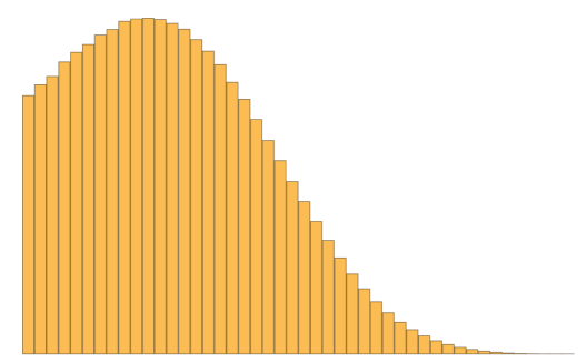
Figure 4. We plot a portion of the weighted histogram of the 6,377,292 values $-\log r$ where $r$ is a circle of generation $n=14$ for standard Apollonian circle packing. There are 46 bins with a weighting corresponding to $r^{\delta}$.

are mutually disjoint (see Figure 4), and that for every $i=1,2,3$:

$$\gamma_{i}(\overline{B}_{i})=g_{4}\circ g_{i}(\overline{B}_{i})=g_{4}(B_{i}^{c})=(g_{4}(B_{i}))^{c}=B_{-i}^{c}$$

we get the following.

Figure 3. Circles, Disks, and Generators of $G$

Observation 20.6.

$\Gamma=\langle\gamma_{1},\gamma_{2},\gamma_{3}\rangle$ is a parabolic Schottky group.

In addition,

Observation 20.7.

The parabolic Schottky group $\Gamma$ has six conjugacy classes of parabolic elements whose representatives are

$$\gamma_{1},\ \ \gamma_{2},\ \ \gamma_{3},\ \ \gamma_{1}\gamma_{2}^{-1},\ \ \gamma_{1}\gamma_{3}^{-1},\ \ \gamma_{2}\gamma_{3}^{-1},$$

with the corresponding parabolic fixed points being the only elements, respectively, of

$$\overline{B}_{1}\cap\overline{B}_{4},\ \ \overline{B}_{2}\cap\overline{B}_{4},\ \ \overline{B}_{3}\cap\overline{B}_{4},\ \ \overline{B}_{-1}\cap\overline{B}_{-2},\ \ \overline{B}_{-1}\cap\overline{B}_{-3},\ \ \overline{B}_{-2}\cap\overline{B}_{-3}.$$

Observation 20.8.

The limit set $\Lambda(\Gamma)$ coincides with the residual set of the Apollonian circle packing generated by the circles $C_{1},C_{2},C_{3},C_{4}$. In addition (see [5], [28], and Theorem 9.6), we have the following.

1. $\delta_{\Gamma}=\text{{\rm HD}}(\Lambda(\Gamma))>1$,

2. $p(g)=1$ for every parabolic element of $\Gamma$, and so

   $$\delta_{\Gamma}>\sup\{p(g)\},$$

   where $g\in\Gamma$ ranges of all parabolic elements of $G$,

3. $\Omega_{\infty}\big{(}\mathcal{S}_{\Gamma}\big{)}=\emptyset$, and so $\mu_{\delta_{\Gamma}}$, the probability $\mathcal{S}_{\Gamma}$-invariant measure on $\Lambda(\Gamma)$, is finite, thus probability after normalization.

Hence, as an immediate consequence of Theorem 20.3, we get the following.

Corollary 20.9.

Let $C_{1},C_{2},C_{3},C_{4}$ be a bounded configuration of four distinct circles in the plane, each of which shares a common tangency point with each of the others. Let $\Gamma$ be the corresponding parabolic Schottky group.

• Let $\delta_{\Gamma}$ be the Poincaré exponent of $\Gamma$; it is known to be equal to $\text{{\rm HD}}(\Lambda(\Gamma))$.

• Let $m_{\delta_{\Gamma}}$ be the Patterson-Sullivan conformal measure for $\Gamma$ on $\Lambda(\Gamma)$.

• Let $\mu_{\delta_{\Gamma}}$ be the probability $\mathcal{S}_{\Gamma}$-invariant measure on $\Lambda(\Gamma)$ equivalent to $m_{\delta_{\Gamma}}$.

• Fix $k\in\{\pm 1,\pm 2,\pm 3\}$ and $\xi\in\Lambda(\Gamma)\cap\overline{B}_{k}$.

Then for every set $Y\subset\overline{B_{k}}$ having at least two distinct points there exists a constant $C_{k}(Y)\in(0,+\infty)$ such that for every Borel set $B\subset{\mathbb{R}}^{d}$ with $m_{\delta_{\Gamma}}(\partial B)=0$ (equivalently $\mu_{\delta_{\Gamma}}(\partial B)=0$), we have that

$$\lim_{T\to+\infty}\frac{N_{\xi}(\Gamma;T,B)}{e^{\delta_{\Gamma}T}}=\frac{\psi_{\delta_{\Gamma}}(\xi)}{\delta_{\Gamma}\chi_{\delta_{\Gamma}}}m_{\delta_{\Gamma}}(B),\ \ \ \ \ \lim_{T\to+\infty}\frac{N_{\xi}(\Gamma;T)}{e^{\delta_{\Gamma}T}}=\frac{\psi_{\delta_{\Gamma}}(\xi)}{\delta_{\Gamma}\chi_{\delta_{\Gamma}}},$$

$$\lim_{T\to+\infty}\frac{N_{p}(\Gamma;T,B)}{e^{\delta_{\Gamma}T}}=\frac{1}{\delta_{\Gamma}\chi_{\delta_{\Gamma}}}\mu_{\delta_{\Gamma}}(B),\ \ \ \ \ \lim_{T\to+\infty}\frac{N_{p}(\Gamma;T)}{e^{\delta_{\Gamma}T}}=\frac{1}{\delta_{\Gamma}\chi_{\delta_{\Gamma}}},$$

$$\lim_{T\to+\infty}\frac{\widehat{N}_{p}(\Gamma;T)}{e^{\delta_{\Gamma}T}} =\frac{1}{\delta_{\Gamma}\chi_{\delta_{\Gamma}}},$$

$$\lim_{T\to+\infty}\frac{D_{\xi}(\Gamma;T,B,Y)}{e^{\delta_{\Gamma}T}} =C(Y)m_{\delta_{G}}(B),$$

$$\lim_{T\to+\infty}\frac{E_{k}(\Gamma;T,B,Y)}{e^{\delta_{\Gamma}T}} =C_{k}(Y)m_{\delta_{\Gamma}}(B),$$

$$\lim_{T\to+\infty}\frac{E_{k}(\Gamma;T,Y)}{e^{\delta_{\Gamma}T}} =C_{k}(Y).$$

Making use of Observation 20.8, as an immediate consequence respectively of Theorem 20.4 and Theorem 20.5, we get the following two theorems.

Theorem 20.10.

Let $C_{1},C_{2},C_{3},C_{4}$ be a bounded configuration of four distinct circles in the plane, each of which shares a common tangency point with each of the others. If $\Gamma$ is the corresponding parabolic Schottky group, then for every $\xi\in\Lambda(\Gamma)$ we have that

$$\lim_{n\to+\infty}\int_{\Gamma_{\xi}^{n}}\frac{\lambda_{\xi}}{n}d\mu_{n}=\chi_{\mu_{\delta}}.$$

The next theorem is a Central Limit Theorem for diameters of circles in the Apollonian Circle Packing.

Theorem 20.11.

Let $C_{1},C_{2},C_{3},C_{4}$ be a bounded configuration of four distinct circles in the plane, each of which shares a common tangency point with each of the others. If $\Gamma$ is the corresponding parabolic Schottky group, then for every $\xi\in\Lambda(\Gamma)$ the sequence of random variables $(\Delta_{n})_{n=1}^{\infty}$ converges in distribution to the normal (Gaussian) distribution $\mathcal{N}_{0}(\sigma)$ with mean value zero and the variance $\sigma^{2}=\text{{\rm P}}_{\mathcal{S}_{\Gamma}^{*}}^{\prime\prime}(\delta)>0$. Equivalently, the sequence $(\mu_{n}\circ\Delta_{n}^{-1})_{n=1}^{\infty}$ converges weakly to the normal distribution $\mathcal{N}_{0}(\sigma^{2})$. This means that for every Borel set $F\subset\mathbb{R}$ with $\hbox{\rm Leb}(\partial F)=0$, we have

$$\lim_{n\to+\infty}\mu_{n}(\Delta_{n}^{-1}(F))=\frac{1}{\sqrt{2\pi}\sigma}\int_{F}e^{-t^{2}/2\sigma^{2}}dt.$$

In Figure 2 we illustate the Central Limit Theorem for the diameters in the standard Apollonian Circle Packing in Theorem 20.5.

Now, we consider the actual counting of the circles in the Apollonian circle packing generated by the bounded configuration of the circles $C_{1},C_{2},C_{3}$ and $C_{4}$. The following immediate observation is crucial to this goal.

Observation 20.12.

The elements of $\mathcal{A}$, the Apollonian circle packing generated by the bounded configuration of the circles $C_{1},C_{2},C_{3},C_{4}$, is bounded and coincide with the following disjoint union

$$\{C_{1},C_{2},C_{3},C_{4}\}\cup\bigcup_{j=1}^{3} (\Gamma_{j}\cup\{\text{{\rm Id}}\})(g_{j}(C_{j}))\cup\bigcup_{j=1}^{3}\bigcup_{i=1,i\neq j}^{4}(\Gamma_{i}\cup\{\text{{\rm Id}}\})(g_{i}\circ g_{j}(C_{j}))\cup$$

$$\cup\{g_{4}(C_{4})\}\cup\cup_{j=1}^{3}(\Gamma_{j}\cup\{\text{{\rm Id}}\})(g_{j}\circ g_{4})(C_{4}),$$

and for $j=1,2,3$ and $i\in\{1,2,3\}\setminus\{j\}$ we have that

$$g_{j}(C_{j})\subset\overline{B}_{j},\ \ g_{i}\circ g_{j}(C_{j})\subset\overline{B}_{i},\ \ g_{4}\circ g_{j}(C_{j})\subset\overline{B}_{-j},\ \ g_{j}\circ g_{4}(C_{4})\subset\overline{B}_{j}.$$

For every $T>0$ and every set $B\subset\mathbb{C}$, we denote

$$\mathcal{D}(T;B):=\big{\{}C\in\mathcal{A}\hbox{ : }-\log\hbox{\text{\rm{diam}}}(C)\leq T\hbox{ and }C\cap B\neq\emptyset\big{\}},$$

$$\mathcal{D}(T):=\mathcal{D}(T;{\mathbb{C}})$$

$$N_{\mathcal{A}}(T;B):=\#\mathcal{D}(T;B)\ \ \hbox{ and }\ \ N_{\mathcal{A}}(T):=\#\mathcal{D}(T).$$

As an immediate consequence of Corollary 20.9 and Observation 20.12 we get the following result proved in [24] (see also [38]–[40]) by entirely different methods.

Theorem 20.13.

Let $C_{1},C_{2},C_{3},C_{4}$ be a bounded configuration of four distinct circles in the plane, each of which shares a common tangency point with each of the others. Let $\mathcal{A}$ be the corresponding circle packing.

Let $\delta=1.30561\ldots$ be the Hausdorff dimension of the residual set of $\mathcal{A}$ and let $m_{\delta}$ be the Patterson-Sullivan measure of the corresponding parabolic Schottky group $\Gamma$.

Then the limit

$$\lim_{T\to+\infty}\frac{N_{\mathcal{A}}(T)}{e^{\delta T}}$$

exists, is positive, and finite. Moreover, there exists a constant $C\in(0,+\infty)$ such that

$$\lim_{T\to+\infty}\frac{N_{\mathcal{A}}(T;B)}{e^{\delta T}}=Cm_{\delta}(B)$$

for every Borel set $B\subset\mathbb{C}$ with $m_{\delta}(\partial B)=0$.

20.3. Apollonian Triangle

Now we consider the Apollonian triangle. Let $C_{1},C_{2},C_{3}$ be three mutually tangent circles in the plane having mutually disjoint interiors. Let $C_{4}$ be the circle tangent to all the circles $C_{1},C_{2},C_{3}$ and having all of them in its interior, i.e. the configuration $C_{1},C_{2},C_{3},C_{4}$ is bounded.

We look at the curvilinear triangle $\mathcal{T}$ formed by the three edges joining the three tangency points of $C_{1},C_{2},C_{3}$ and lying on these circles. The bounded collection

$$\mathcal{G}:=\{C\in\mathcal{A}\hbox{ : }C\subset\mathcal{T}\}$$

is called the Apollonian gasket generated by the circles $C_{1},C_{2},C_{3}$. Since $\partial\mathcal{T}\cap\Lambda(\Gamma)=\partial\mathcal{T}$ has Hausdorff dimension $1$, since $\delta>1$ and since $m_{\delta}$ is a constant multiple of $\delta$–dimensional Hausdorff measure restricted to $\Lambda(\Gamma)$, we have that $m_{\delta}(\partial T)=0$. Another, a more general argument for this, would be to invoke Corollary 1.4 from [11]. Therefore, as an immediate consequence of Theorem 20.13 we get the following result, also proved by Kontorovich and Oh in [24] (see also [38]–[40]) with entirely different methods.

Corollary 20.14.

Let $C_{1},C_{2},C_{3}$ be three mutually tangent circles in the plane having mutually disjoint interiors. Let $C_{4}$ be the circle tangent to all the circles $C_{1},C_{2},C_{3}$ and having all of them in its interior, i.e. the configuration $C_{1},C_{2},C_{3},C_{4}$ is bounded. Let $\mathcal{A}$ be the corresponding (bounded) circle packing.

Let $\delta=1.30561\ldots$ be the Hausdorff dimension of the residual set of $\mathcal{A}$ and let $m_{\delta}$ be the Patterson-Sullivan measure of the corresponding parabolic Schottky group $\Gamma$.

If $\mathcal{T}$ is the curvilinear triangle formed by $C_{1}$, $C_{2}$ and $C_{3}$, then the limit

$$\lim_{T\to+\infty}\frac{N_{\mathcal{A}}(T;\mathcal{T})}{e^{\delta T}}$$

exists, is positive, and finite; we just count the elements of $\mathcal{G}$. Moreover, there exists a constant $C\in(0,+\infty)$, in fact the one of Theorem 20.13, such that

$$\lim_{T\to+\infty}\frac{N_{\mathcal{A}}(T;B)}{e^{\delta T}}=Cm_{\delta}(B)$$

for every Borel set $B\subset\mathcal{T}$ with $m_{\delta}(\partial B)=0$.

Now we will provide a somewhat different proof of Corollary  20.14, by appealing directly to the theory of parabolic conformal IFSs and avoiding the intermediate step of parabolic Schottky groups. Indeed, let $C_{0}$ be the circle inscribed in $\mathcal{T}$ and tangent to the circles $C_{1}$, $C_{2}$ and $C_{3}$. Let $x_{1},x_{2}$ and $x_{3}$ be the vertices of the curvilinear triangle $\mathcal{T}$, i.e., for $i=1,2,3$, $x_{i}$ is the only element of the intersection $K_{i}\cap K_{4}$. Let

$$\varphi_{i}:\widehat{\mathbb{C}}\to\widehat{\mathbb{C}}$$

be the Möbius transformation fixing the point $x_{i}$ and mapping the other vertices $x_{j}$ and $x_{k}$, respectively, onto the only points of the intersections $C_{0}\cap C_{j}$ and $C_{0}\cap C_{k}$. Then

$$\mathcal{S}=\{\varphi_{1},\varphi_{2},\varphi_{3}\}$$

is a parabolic IFS defined on $\overline{B}_{4}$, $x_{i}$ is a parabolic fixed point of $\varphi_{i}$, $i=1,2,3$, and

$$\mathcal{G}=\{\varphi_{\omega}(C_{0})\hbox{ : }\omega\in\{1,2,3\}^{*}\},$$

see Figure 5. We therefore obtain Corollary 20.14 immediately from Theorem 12.6.

Figure 5. Apollonian Triangle

Remark 20.15.

In the context of limit sets, such as circle packings, there is scope for finding error terms in the above asymptotic formulae, see ex. [26] and [43]. It could also done using the techniques worked out in our present manuscript. However, in the general setting of conformal graph directed Markov systems quite delicate technical hypotheses might well be required.

Remark 20.16.

For these analytic maps it would be equally possible to work with Banach spaces of analytic functions, rather than Hölder continuous functions. This would have the advantage that the transfer operator operator is compact (even trace class or nuclear) and might help to simplify some of the arguments as well as being useful in explicit numerical computations. On the other hand, working with Hölder functions allows the results to be applied to a far greater range of examples.

Remark 20.17.

In higher dimensions, we can consider the packing of the sphere $S^{d}$ by mutually tangent $d$-spheres. The same analysis gives a corresponding asymptotic for the diameters of spheres. In an overlapping setting and with entirely different metods this question has been addressed in Oh’s paper [37].

21. Fuchsian Groups

We recall that a Fuchsian group $\Gamma$ is a discrete group of orientation preserving Poincaré isometries acting on the unit disk

$$\mathbb{D}=\{z\in\mathbb{C}\hbox{ : }|z|<1\}$$

in the complex plane. A Poincaré isometry means that the Poincaré metric

$$\frac{|dz|}{1-|z|^{2}}$$

is preserved, equivalently the map is a holomorphic homeomorphism of the disk $\mathbb{D}$ onto itself. The limit set $\Lambda(\Gamma)$ of $\Gamma$ is a compact perfect subset of $S^{1}=\partial\mathbb{D}=\{z\in\mathbb{C}\hbox{ : }|z|=1\}$. Assume that $\Gamma$ is finitely generated and denote a minimal (in the sense of inclusion) set of its generators by $\{g_{j}\}_{j=\pm 1}^{\pm q}$ where $g_{j}=g_{j}^{-1}$. Assume that $q\geq 2$, so that $\Gamma$ is non-elementary. Following [53] (see also [54]) we call $\Gamma$ non-exceptional if at least one of the following conditions holds (corresponding to conditions (10.1)-(10.3) from [25]):

1. $\mathbb{D}/\Gamma$ is not compact;

2. The generating set has at least $5$ elements (i.e., $q\geq 5$) and every non-trivial relation has length $5$; and

3. At least $3$ of the generating relations have length at least $7$.

In particular finitely generated every parabolic Fuchsian group is non-exceptional as the condition (1) above is satisfied. In the language of conformal GDMSs, C. Series proved in [53] (see also [54]) the following:

Theorem 21.1.

If $\Gamma$ is a non-exceptional Fuchsian group then there exists a finite irreducible pre-parabolic GDMS $\mathcal{S}_{\Gamma}$ with an incidence matrix $A$, a finite set of vertices $V$ and a finite alphabet $E=\{\pm 1,\pm 2,\cdots,\pm q\}$ such that

1. For every $j\in E$ the corresponding element of $\mathcal{S}_{\Gamma}$ is $g_{j}:X_{t(j)}\to X_{i(j)}$

2. All sets $X_{v}$, $v\in V$ are closed subarcs of $S^{1}$

3. The map $E_{A}^{*}\ni\omega\mapsto g_{\omega}\in\Gamma$ is a bijection

4. $\Lambda(\Gamma)=\mathcal{J}_{\mathcal{S}_{\Gamma}}$

5. The map $\pi_{\mathcal{S}_{\Gamma}}:E_{A}^{\infty}\to\mathcal{J}_{\mathcal{S}_{\Gamma}}=\Lambda(\Gamma)$ is a continuous surjection and it is $1$-to-$1$ except at countably many points, where it is $2$-to-$1$.

Similarly to (but not exactly) as in Section 19, given $e\in E$ we define

$$\Gamma_{e}:=\{\gamma\omega\in E_{A}^{*}\ \hbox{ and }\ \omega_{1}=e\}.$$

Then having $\rho\in A_{A}^{\mathbb{N}}$ we set

$$\Gamma_{\rho}:=\Gamma_{\rho_{1}}$$

Again, similarly as in Section 19, we denote

$$\lambda_{\rho}(\gamma)=-\log|\gamma^{\prime}(\pi_{\Gamma}(\rho))|=-\log|\gamma_{\omega}^{\prime}(\pi_{\Gamma}(\omega))|=\lambda_{\rho}(\omega)$$

for every $\omega\in E^{*}_{\rho}$ ($\gamma=\gamma_{\omega}\in\Gamma_{\rho_{1}}=\Gamma_{\rho}$) and

$$\Delta(Y):=-\log(\hbox{\rm diam}(\gamma_{\omega}(Y)))$$

if $Y\subset X_{t(\rho_{1})}$. Also

$$\lambda_{p}(\omega)=-\log|\gamma_{\omega}^{\prime}(x_{\omega})|$$

if $\omega\in E_{p}^{*}$

Let $B$ denote a Borel subset of the set $S^{1}$. Set

$$\pi_{\rho}(\Gamma;T,B):=\{\gamma\in\Gamma_{\rho}\hbox{ : }\lambda_{\rho}(\gamma)\leq T\hbox{ and }\gamma(\pi_{\Gamma}(\rho))\in B\}$$

$$\pi_{\rho}(\Gamma;T):=\pi_{\xi}(\Gamma;T,S^{1})=\{\gamma\in\Gamma_{\rho}\hbox{ : }\lambda_{\rho}(\gamma)\leq T\}$$

$$\pi_{p}(\Gamma;T,B):=\{\omega\in E_{p}^{*}\hbox{ : }\lambda_{p}(\omega)=l(\gamma_{\omega})\leq T\hbox{ and }x_{\omega}\in B\},$$

$$\pi_{p}(\Gamma;T):=\pi_{p}(\Gamma;T,S^{1})=\{\omega\in E_{p}^{*}\hbox{ : }\lambda_{p}(\omega)=l(\gamma_{\omega})\leq T\},$$

$$\widehat{\pi}_{p}(\Gamma,T):=\{\gamma\in\widehat{\Gamma}\hbox{ : }l(\gamma_{\gamma})\leq T\}$$

With $e:=\rho_{1}$ we further denote

$$\mathcal{D}_{\rho}(\Gamma;T,B,Y):=\{\gamma\in\Gamma_{e}\hbox{ : }\Delta_{\gamma}(Y)\leq T\ \hbox{ and }\ \gamma(\pi_{\Gamma}(\rho))\in B\},$$

$$\mathcal{E}_{e}(\Gamma;T,B,Y)=\{\gamma\in\Gamma_{e}\hbox{ : }\Delta_{\gamma}(Y)\leq T\ \hbox{ and }\ \gamma(Y)\cap B\neq\emptyset\},$$

and

$$\mathcal{E}_{e}(\Gamma;T,Y):=\mathcal{E}_{e}(\Gamma;T,S^{1},Y)=\{\gamma\in\Gamma_{e}\hbox{ : }\Delta_{\gamma}(Y)\leq T\}.$$

We denote by $N_{\xi}(\Gamma;T,B)$, $N_{\xi}(\Gamma;T)$, $N_{p}(\Gamma;T,B)$, $N_{p}(\Gamma;T)$, $\widehat{N}_{p}(\Gamma;T)$, $D_{\xi}(\Gamma;T,B,Y)$, $E_{e}(\Gamma;T,B,Y)$ and $E_{e}(\Gamma;T,Y)$ the corresponding cardinalities.

As immediate consequences of Theorem 5.9, Theorem 8.1, Theorem 8.4, Theorems 11.2, 12.1, and 12.2, along with Theorem 21.1 and Fuchsian counterparts of Proposition 19.5, Observation 19.6 and Proposition 19.8, following from [53] and [54], we get the following.

Theorem 21.2.

Let $\Gamma=\langle\gamma_{j}\rangle_{j=1}^{q}$ be a finitely generated non-exceptional Fuchsian group.

• Let $\delta_{\Gamma}$ be the Poincaré exponent of $\Gamma$; it is known to be equal to $\text{{\rm HD}}(\Lambda(\Gamma))$.

• Let $m_{\delta_{\Gamma}}$ be the Patterson-Sullivan conformal measure for $G$ on $\Lambda(\Gamma)$.

• Let $\mu_{\delta_{\Gamma}}$ be the $\mathcal{S}_{\Gamma}$-invariant measure on $\Lambda(\Gamma)$ equivalent to $m_{\delta_{\Gamma}}$.

• Fix $e\in E=\{\pm 1,\pm 2,\cdots,\pm q\}$ and $\rho\in E_{A}^{\infty}$ with $\rho_{1}=e$.

Let $B\subseteq S^{1}$ be a Borel set with $m_{\delta_{\Gamma}}(\partial B)=0$ (equivalently $\mu_{\delta_{\Gamma}}(\partial B)=0$) and let $Y\subseteq X_{t(e)}$ be a set having at least two distinct points. Then with some constant $C_{e}(Y)\in(0,+\infty]$, we have that

$$\lim_{T\to+\infty}\frac{N_{\xi}(\Gamma;T,B)}{e^{\delta_{\Gamma}T}}=\frac{\psi_{\delta_{\Gamma}}(\xi)}{\delta_{\Gamma}\chi_{\delta_{\Gamma}}}m_{\delta_{\Gamma}}(B),\ \ \ \ \ \lim_{T\to+\infty}\frac{N_{\xi}(\Gamma;T)}{e^{\delta_{\Gamma}T}}=\frac{\psi_{\delta_{\Gamma}}(\xi)}{\delta_{\Gamma}\chi_{\delta_{\Gamma}}},$$

$$\lim_{T\to+\infty}\frac{N_{p}(\Gamma;T,B)}{e^{\delta_{\Gamma}T}}=\frac{1}{\delta_{\Gamma}\chi_{\delta_{\Gamma}}}\mu_{\delta_{\Gamma}}(B),\ \ \ \ \ \lim_{T\to+\infty}\frac{N_{p}(\Gamma;T)}{e^{\delta_{\Gamma}T}}=\frac{1}{\delta_{\Gamma}\chi_{\delta_{\Gamma}}},$$

$$\lim_{T\to+\infty}\frac{\widehat{N}_{p}(\Gamma;T)}{e^{\delta_{\Gamma}T}} =\frac{1}{\delta_{\Gamma}\chi_{\delta_{\Gamma}}},$$

$$\lim_{T\to+\infty}\frac{D_{\xi}(\Gamma;T,B,Y)}{e^{\delta_{\Gamma}T}} =C_{e}(Y)m_{\delta_{\Gamma}}(B),$$

$$\lim_{T\to+\infty}\frac{E_{k}(\Gamma;T,B,Y)}{e^{\delta_{\Gamma}T}} =C_{e}(Y)m_{\delta_{\Gamma}}(B),$$

$$\lim_{T\to+\infty}\frac{E_{k}(\Gamma;T,Y)}{e^{\delta_{\Gamma}T}} =C_{e}(Y).$$

In addition, $C_{e}(Y)>0$ is finite if and only if

$$\overline{Y}\cap\Omega(\mathcal{S}_{\Gamma})=\emptyset,$$

in particular if $\Gamma$ has no parabolic points, i.e. if it is convex co-compact.

Theorem 13.1 – Theorem 13.3 hold for the conformal GDMS $\mathcal{S}_{\Gamma}$, associated to the group $\Gamma$, without changes. Therefore, we do not repeat them here. However, as in Section 19, we present the appropriate versions of Theorems 15.1 and 15.2 as their formulations are closer to the group $\Gamma$. In order to get appropriate expressions in the language of the group $\Gamma$ itself, given $\rho\in E_{A}^{\infty}$, and an integer $n\geq 1$, we set

$$\Gamma_{\rho}^{n}:=\{\gamma_{\omega}:\omega\in E_{\rho}^{n}\}\subseteq\Gamma_{\rho}.$$

Furthermore, we define a probability measure $\mu_{n}$ on $\Gamma_{\rho}^{n}$ by setting that

(21.1) $$\mu_{n}(H):=\frac{\sum_{\gamma\in H}e^{-\delta\lambda_{\rho}(\gamma)}}{\sum_{\gamma\in\Gamma_{\rho}^{n}}e^{-\delta\lambda_{\rho}(\gamma)}}$$

for every set $H\subset\Gamma_{\rho}^{n}$. As an immediate consequence of Theorem 15.1 we get the following.

Theorem 21.3.

If $\Gamma=\langle\gamma_{j}\rangle_{j=1}^{q}$ is a finitely generated non-exceptional convex co-compact (i. e. without parabolic fixed points) Fuchsian group, then for every $\rho\in E_{A}^{\infty}$ we have that

$$\lim_{n\to+\infty}\int_{\Gamma_{\rho}^{n}}\frac{\lambda_{\rho}}{n}d\mu_{n}=\chi_{\mu_{\delta}}.$$

Now define the functions $\Delta_{n}:\Gamma_{\rho}^{n}\to\mathbb{R}$ by the formulae

$$\Delta_{n}(\gamma)=\frac{\lambda_{\xi}(\gamma)-\chi n}{\sqrt{n}}.$$

As an immediate consequence of Theorem 15.2 we get the following.

Theorem 21.4.

If $\Gamma=\langle\gamma_{j}\rangle_{j=1}^{q}$ is a finitely generated non-exceptional convex co-compact (i. e. without parabolic fixed points) Fuchsian group, then for every $\rho\in E_{A}^{\infty}$ the sequence of random variables $(\Delta_{n})_{n=1}^{\infty}$ converges in distribution to the normal (Gaussian) distribution $\mathcal{N}_{0}(\sigma)$ with mean value zero and the variance $\sigma^{2}=\text{{\rm P}}_{\mathcal{S}_{\Gamma}}^{\prime\prime}(\delta)>0$. Equivalently, the sequence $(\mu_{n}\circ\Delta_{n}^{-1})_{n=1}^{\infty}$ converges weakly to the normal distribution $\mathcal{N}_{0}(\sigma^{2})$. This means that for every Borel set $F\subset\mathbb{R}$ with $\hbox{\rm Leb}(\partial F)=0$, we have

(21.2) $$\lim_{n\to+\infty}\mu_{n}(\Delta_{n}^{-1}(F))=\frac{1}{\sqrt{2\pi}\sigma}\int_{F}e^{-t^{2}/2\sigma^{2}}dt.$$

21.1. Hecke Groups

A special class of Fuchsian parabolic (so non-exceptional) groups are Hecke groups. These are easiest to express in the Lobachevsky model of hyperbolic geometry and plane rather than in the Poincaré one. The 2-dimensional hyperbolic (Lobachevsky) plane is the set

$${\mathbb{H}}:=\{z\in{\mathbb{C}}:\text{{\rm Im}}z>0\}$$

endowed with the Riemannian metric

$$\frac{|dz|}{\text{{\rm Im}}z}.$$

Given $\varepsilon>0$ the corresponding Hecke group is defined as follows

$$\Gamma_{\epsilon}:=\big{\langle}z\mapsto-1/z,\,z\mapsto z+1+\epsilon\big{\rangle}.$$

This group has an elliptic element order $2$ which is the map $z\longmapsto-1/z$ and one (conjugacy class) of parabolic elements which is the map $z\longmapsto z+1+\epsilon$. Its (parabolic) fixed point is $\infty$. In particular all the limit sets $\Lambda(\Gamma_{\varepsilon})$ are unbounded, and therefore the Hecke groups $\Gamma_{\varepsilon}$ do not really fit into the setting of our current manuscript. However, any Möbius transformation

$$H:{\mathbb{D}}\to{\mathbb{H}}$$

is an isometry with respect to corresponding Poincaré metrics and the map

$$\Gamma_{\varepsilon}\ni\gamma\longmapsto H^{-1}\circ\gamma\circ H$$

establishes an algebraic isomorphism between $\Gamma_{\varepsilon}$ and the group

$$\hat{\Gamma}_{\varepsilon}:=\{H^{-1}\circ\gamma\circ H:\gamma\in\Gamma_{e}\}.$$

Of course, the conjugacy $H$ between $\hat{\Gamma}_{\varepsilon}$ and $\Gamma_{\varepsilon}$ congregates elements of $\hat{\Gamma}_{\varepsilon}$ and $\Gamma_{\varepsilon}$ viewed as isometric actions. The groups $\hat{\Gamma}_{\varepsilon}$ are Fuchsian parabolic (so non-exceptional) groups acting on ${\mathbb{D}}$ and perfectly fit into the setting of Section 21. In particular, Theorem 21.2 holds for them.

References

- [1] J. Aaronson, M. Denker, M. Urbański, Ergodic theory for Markov fibered systems and parabolic rational maps, Transactions of A.M.S. 337 (1993), 495-548.
- [2] P. Arnoux and S. Starosta, The Rauzy Gasket, in Further Developments in Fractals and Related Fields (Part of the series Trends in Mathematics), (2013), 1-23.
- [3] A. Avila, P. Hubert, A. Skripchenko, On the Hausdorff dimension of the Rauzy gasket, Preprint 2013.
- [4] R. Bowen, Equlibrium states and the ergodic theory of Anosov diffeomorphisms, Lect. Notes in Math. 470 (1975), Springer Verlag.
- [5] D. Boyd, The sequence of radii of the Apollonian packing. Math. Comp. 39 (1982), no. 159, 249–254.
- [6] S. Bullett and G. Mantica: Group theory of hyperbolic circle packings, Nonlinearity 5, (1992), 1085-1109.
- [7] V. Chousionis, J. Tyson, M. Urbański, Conformal graph directed Markov systems on Carnot groups, Preprint 2016.
- [8] J. Conway, Functions of Complex Variable II, Springer-Verlag, New York, 1995.
- [9] M. Denker, M. Urbański, Hausdorff and conformal measures on Julia sets with a rationally indifferent periodic point, J. London Math. Soc. 43 (1991), 107-118.
- [10] M. Denker, M. Urbański, On absolutely continuous invariant measures for expansive rational maps with rationally indifferent periodic points, Forum Math. 3(1991), 561-579.
- [11] L. Flaminio and R. J. Spatzier, Geometrically fnite groups, Patterson-Sullivan measures and Ratner’s rigidity theorem, Invent. Math., 99 (1990),601-626.
- [12] E. Fuchs, Notes on Apollonian Circle Packings (SWIM), http://www.math.princeton.edu/efuchs/
- [13] R.L. Graham, J.C. Lagarias, C.L. Mallows, A.R. Wilks, C.H. Yan, Apollonian circle packings: geometry and group theory. I. The Apollonian group, Journal of Number Theory, 100 (2003), 1-45.
- [14] S. Gouëzel, Berry-Esseen theorem and local limit theorem for non uniformly expanding maps, Ann. I. Poincaré Probabilités et Statistiques, 41 (2005) 997-1024
- [15] S. Gouëzel, Local limit theorem for nonuniformly partially hyperbolic skew-products and Farey sequences, Duke Mathematical Journal 147:192-284, 2009.
- [16] S. Gouëzel, Statistical properties of a skew product with a curve of neutral points, Ergod. Th. and Dynam. Sys., 27 (2007), 123–151.
- [17] S. Gouëzel, Central limit theorem and stable laws for intermittent maps, Probab. Theory and Related Fields, 128 (2004), 82–122.
- [18] R. Graham, J. Lagarias, C. Mallows, A. Wilks, C, Yan, Apollonian circle packings: number theory, J. Number Theory 100 (2003) 1-45.
- [19] P. Hanus, D. Mauldin, and M. Urbański, Thermodynamic formalism and multifractal analysis of conformal infinite iterated function systems, Acta Math. Hungarica, 96 (2002), 27-98.
- [20] B. Heersink, Distribution of the Periodic Points of the Farey Map, Preprint 2017.
- [21] E. Hille, Analytic Function Theory Volume II, AMS Chelsea Publishing, Providence, Rhode Island, 1962.
- [22] H. Hu, Equilibriums of some non-Holder potentials, Transactions of the American Mathematical Society, 360 (2008), 2153-2190
- [23] T. Iwaniec, G. Martin, Geometric Function Theory and Non-linear Analysis, Clarendon Press, Oxford, 2001.
- [24] A. V. Kontorovich and H. Oh, Apollonian Circle Packings and Closed Horospheres on Hyperbolic 3-Manifolds, Journal of the American Mathematical Society 24 (2011), 603-648.
- [25] S. Lalley, Renewal theorems in symbolic dynamics, with applications to geodesic flows, noneuclidean tesselations and their fractal limits, Acta. Math. 163 (1989), 1-55.
- [26] M. Lee, H. Oh, Effective circle count for Apollonian packings and closed horospheres, GAFA, 23 (2013), 580–621.
- [27] D. Mauldin and M. Urbański, Dimensions and measures in infinite iterated function systems, Proc. London Math. Soc. (3) 73 (1996) 105-154.
- [28] D. Mauldin and M. Urbański, Dimension and measures for a curvilinear Sierpinski gasket or Apollonian packing, Adv. Math., 136 (1998), no. 1, 26-38.
- [29] D. Mauldin and M. Urbański, Conformal iterated function systems with applications to the geometry of continued fractions, Transactions of A.M.S. 351 (1999), 4995-5025.
- [30] D. Mauldin and M. Urbański, Parabolic iterated function systems, Ergod. Th. & Dynam. Sys. 20 (2000), 1423-1447.
- [31] D. Mauldin and M. Urbański, Gibbs states on the symbolic space over an infinite alphabet, Israel. J. of Math., 125 (2001), 93-130.
- [32] D. Mauldin and M. Urbański, Graph Directed Markov Systems: Geometry and Dynamics of Limit Sets, Cambridge University Press (2003).
- [33] I. Melbourne and A. Torok, Statistical limit theorems for suspension flows. Israel J. Math. 144 (2004), 191–209.
- [34] D. Mumford, C. Series and D. Wright, Indra’s Pearls: The Vision of Felix Klein, Cambridge University Press 2002.
- [35] F. Naud, Expanding maps on Cantor sets and analytic continuation of zeta functions, Ann of ENS, 38, (2005), p. 116-153.
- [36] R. D. Nussbaum, The radius of the essential spectrum, Duke Math. J. 37 (1970), 473-478.
- [37] H. Oh, Harmonic analysis, Ergodic theory and Counting for thin group, In ”Thin groups and superstrong approximation”, edited by Breuillard and Oh, MSRI publ.61 Cambridge Univ. Press, 2014.
- [38] H. Oh and N. Shah, Equidistribution and Counting for orbits of geometrically finite hyperbolic groups, Journal of AMS 26 (2013), 511-562.
- [39] H. Oh and N. Shah, Counting visible circles on the sphere and Kleinian groups, preprint (2010).
- [40] H. Oh and N. Shah, The asymptotic distribution of circles in the orbits of Kleinian groups, Inventiones Math. 187 (2012), 1-35.
- [41] J. Parker, Kleinian circle packings, Topology 34 (1995), 489-496.
- [42] I. D. Morris, A rigorous version of R. P. Brent’s model for the binary Euclidean algorithm, Preprint 2014.
- [43] W. Pan, Effective equidistribution of circles in the limit sets of Kleinian groups, Journal of Modern Dynamics, 11 (2017), 189–217.
- [44] W. Parry and M. Pollicott, An analogue of the prime number theorem for closed orbits of Axiom A flows. Annals of Math. 118 (1983), 573–591.
- [45] W. Parry and Mark Pollicott, Zeta functions and the periodic orbit structure of hyperbolic dynamics, Asterisque 268, (1990).
- [46] M. Pollicott, A complex Ruelle-Perron-Frobenius theorem and two counterexamples, Ergod. Th. & Dynam. Sys. 4 (1984), 135-146.
- [47] M. Pollicott, Meromorphic Extensions for Generalized Zeta Functions, Inventiones Math. 85 (1986), 147-164.
- [48] M. Pollicott, R. Sharp, Exponential error terms for Growth functions on negatively curved surfaces, Amer. J. Math. 120 (2008), 1019-1042.
- [49] F. Przytycki, M. Urbański, Rigidity of tame rational functions, Bull. Pol. Acad. Sci., Math., 47.2 (1999), 163-182.
- [50] F. Przytycki, M. Urbański, Conformal Fractals — Ergodic Theory Methods, Cambridge University Press 2010.
- [51] D. Ruelle, Thermodynamic formalism, Encycl. Math. Appl. 5, Addison-Wesley 1978.
- [52] P. Sarnak, ”Integral Apollonian Packings”, MAA Lecture – January, 2009.
- [53] C. Series, Geometrical Markov coding of geodesics on surfaces of constant negative curvature, Ergodic Theory Dynam. Systems 6.4 (1986) 601–625.
- [54] C. Series, The infinite word problem and limit sets in fuchsian groups. Ergodic Theory Dynamical Systems, 1 (1981), 337-360.
- [55] D. Sullivan, Quasiconformal homeomorphisms in dynamics, topology and geometry, Prof. International Congress of Mathematicians, 1986 1216–1228.
- [56] T. Szarek, M. Urbański, and A. Zdunik, Continuity of Hausdorff Measure for Conformal Dynamical Systems, Discrete and Continuous Dynamical Systems, Series A., 33 (2013), 4647–4692.
- [57] M. Urbański, On Hausdorff dimension of Julia set with a rationally indifferent periodic point, Studia Math. 97 (1991), 167 – 188.
- [58] M. Urbański, Parabolic Cantor sets, Fund. Math. 151 (1996), 241-277.
- [59] M. Urbański, Hausdorff measures versus equilibrium states of conformal infinite iterated function systems, Periodica Math. Hung., 37 (1998), 153-205.
- [60] P. Walters, An introduction to ergodic theory, Springer 1982.
- [61] N. Wiener, Fourier Integral and Certain of Its Applications, Dover, 1959.
- [62] L.-S. Young. Statistical properties of dynamical systems with some hyperbolicity. Ann. of Math., 147 (1998) 585–650.
- [63] L.-S. Young, Recurrence times and rates of mixing, Israel J. Math., 110 (1999), 153-188.
- [64] A. Zdunik, Parabolic orbifolds and the dimension of maximal measure for rational maps, Inv. Math. 99 (1990), 627-649.