Vaidya Spacetime in the Diagonal Coordinates
Abstract
We have analyzed the transformation from initial coordinates of the Vaidya metric with light coordinate to the most physical diagonal coordinates . An exact solution has been obtained for the corresponding metric tensor in the case of a linear dependence of the mass function of the Vaidya metric on light coordinate . In the diagonal coordinates, a narrow region (with a width proportional to the mass growth rate of a black hole) has been detected near the visibility horizon of the Vaidya accreting black hole, in which the metric differs qualitatively from the Schwarzschild metric and cannot be represented as a small perturbation. It has been shown that, in this case, a single set of diagonal coordinates is insufficient to cover the entire range of initial coordinates outside the visibility horizon; at least three sets of diagonal coordinates are required, the domains of which are separated by singular surfaces on which the metric components have singularities (either or .). The energy-momentum tensor diverges on these surfaces; however, the tidal forces turn out to be finite, which follows from an analysis of the deviation equations for geodesics. Therefore, these singular surfaces are exclusively coordinate singularities that can be referred to as false firewalls because there are no physical singularities on them. We have also considered the transformation from the initial coordinates to other diagonal coordinates , in which the solution is obtained in explicit form, and there is no energy-momentum tensor divergence.
1 INTRODUCTION
The Vaidya metric describes the spacetime produced by a spherically symmetric radial radiation flow. This metric has the form Vaidya43 ; Vaidya51 ; Vaidya53
| (1) |
In particular, the Vaidya metric describes a nonstationary accreting or emitting black hole. In this metric, is an arbitrary mass function that depends (in the case of accretion) on coordinate , where is the advanced light coordinate or (in the case of emission of radiation) on coordinate , where is the retarded light coordinate. For , metric (1) describes a Schwarzschild black hole of mass . Here and below, we are using units of measurement in which for the velocity of light and for the gravitational constant.
Vaidya metric (1), which is one of a few known exact solutions in the general theory of relativity, has a large number of astrophysical and theoretical applications. In particular, it is used to describe the quantum evaporation of black holes VolZagFro76 ; Hiscock81 ; Kuroda84 ; Beciu84 ; Kaminaga90 ; Zheng94 ; Farley06 ; Sawayama06 or the emission of radiation by astrophysical objects Knutsen84 ; Barreto93 ; Adams94 ; Maharaj02 ; Sungwook10 ; Alishahiha14 . This metric is also employed in investigations of gravitational collapse and the formation of naked singularities HiscockWilliamsEardley ; Kuroda84b ; Papapetrou85 ; WauLak86b ; Dwivedi89 ; Dwivedi91 ; Joshi92 ; Joshi92b ; Joshi93 ; Dwivedi95 ; Ghosh01 ; Mkenyeleye14 . However, the interpretation of physical results obtained in this metric is complicated because this metric is written in terms of coordinates , where is not a directly measurable physical quantity. It is known that, in some simple cases, the expressions that describe the transition to double zero coordinates can be derived WauLak86 , but a transition to more physical diagonal coordinates involves analytic difficulties, and the explicit form of the corresponding coordinate transformation is generally unknown LinSchMis65 .
In this study, we analyze the coordinate transformations from the standard coordinates of the Vaidya metric to diagonal coordinates in the case of a linear mass function , , where parameter characterizes the accretion or emission rate. Using this Ansatz, we solve the problem of transforming the Vaidya metric to the diagonal coordinates fully analytically by calculating all metric coefficients. Vaidya metric (1) with a linear mass function has been considered previously in a large number of publications in various aspects VolZagFro76 ; Hiscock81 ; LevinOri ; Shao05 ; AbdallaChirenti ; YangJeng06 ; BengtssonSenovilla09 . However, the form of the Vaidya metric in diagonal coordinates was not obtained in these publications. We obtained the first such solution in we , where special diagonal coordinates were used (these coordinates will be considered in Section 3) below). In this work, we will also obtain the solution for another (more physical) choice of diagonal coordinates .
The transition to the diagonal coordinates makes the Vaidya problem closer to the actual situation because these coordinates correspond to the results of physical measurements that could have been taken by a static observer. Using the diagonal coordinates, it is clear how the accretion process is seen by the static observer of a black hole or, in a more general form, the physical structure of space-time in the presence of a radial radiant flux. Therefore, this formulation of the problem is extremely close to the physically realizable situation.
It turned out that, even in the region beyond the gravitational radius , in the -region, a single set of diagonal coordinates or is insufficient to cover the entire range of variations in initial coordinates in metric (1), but several sets of diagonal coordinates are required, the ranges of variations in which are separated by surfaces with singularities of the metric (either or ). These sets served as the charts that cover the entire manifold with allowance for physical limitation . At the boundaries of these charts, the energy-momentum tensor experiences a divergence, which, however, is not associated with the presence of physical caustics in the distribution of accreted radiation. Analysis of the deviation equations of geodesics shows that tidal forces on the boundary surfaces are finite; therefore, these surfaces are physically coordinate singularities that can be referred to as false firewalls.
Initial Vaidya metric (1) is geodetically incomplete and requires analytic expansion for describing the global geometry of space-time. One of the expansions was proposed by Izrael Israel67 in general form for the global geometry of eternal space-time with infinite ladders of black and white holes. Other approaches were used in Kuroda84 ; Fayosyx95 , in which additional spacetime regions were constructed, as well as in HiscockWilliamsEardley ; Krori74 ; Waugh86 , where special mass fractions were employed. The application of new diagonal coordinates enabled us to reveal the global structure of the space-time for the Vaidya metric with linear mass function . The main instruments of analysis are exact expressions for the radial light geodesics. As a result, we have constructed a geodetically complete (with physical limitation ) space-time and the corresponding conformal Carter–Penrose diagrams.
2 VAIDYA METRIC IN DIAGONAL COORDINATES
In this section, we choose coordinates of curvatures as diagonal coordinates, in which the metric has the form LL-2
| (2) |
or, after the redefinition of the coefficients for convenience,
| (3) |
where and are certain functions that can be determined from the Einstein equations. Let us introduce mass function connected by definition with and by the following relation:
| (4) |
2.1 Transition to Diagonal Coordinates
We will seek the transformation of coordinates of the initial Vaidya metric to diagonal coordinates as follows:
| (5) |
Substituting these relations into (1) and equating the resulting coefficients to the corresponding coefficients in Eq. (3), we obtain the system of equations
| (6) |
We write the second of these equations in the form
| (7) |
and multiply it by :
| (8) |
We consider the linear mass function
| (9) |
In the case of accretion, we have and . In the case of emission, we obtain and . Consequently, for both cases, and . Then, Eq. (8) assumes the form
| (10) |
Denoting
| (11) |
we write the solution to Eq. (10) in the following
implicit form:
| (12) |
Let us first consider the case when . Evaluating the integral in Eq. (12), we obtain
| (13) |
where the following notation has been introduced:
| (14) |
and
| (15) |
and is a certain as yet unknown function.
Let us now find coefficient . Differentiating Eq. (13) with respect to and substituting
| (16) |
we obtain
| (17) |
Function has singular points and ; therefore, the entire domain splits into four parts as follows:
| (18) |
in each of which we must carry out separate calculations. It should be noted that free parameters and can be different in different regions, and the relation between them must be established by joining the solution. The time can be redefined as follows: ; therefore, we can choose
| (19) |
where the sign in each specific case is determined from the condition as follows:
| (20) |
In all domains (18), we obtain the same expression from Eqs. (6) as follows:
| (21) |
Thus, we have determined all metric coefficients in parametric form as (21), , and (13), where is a parameter.

The differential transformation to new coordinates has the form
| (22) |
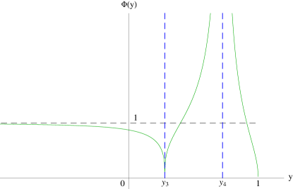
It was noted in LinSchMis65 that the expression for the differential analogous to (22) could have been obtained by evaluating the integrating factor. It is important that in the new metric is a function of only; i.e., , where . Figure 1 shows the sections of function (in the case of accretion) by planes.
Let us consider the limiting transition to the Schwarzschild metric for . In Fig. 1, the Schwarzschild metric is above point B; therefore, asymptotically flat infinity is outside the thick shell. Within the shell, between points A and B, we have , , , and for ; hence, expression (21) has the asymptotic form (it should be recalled that ) as follows:
| (23) |
At any radius for , we obtain and, ultimately, , i.e., the Schwarzschild metric. The deviation of the Schwarzschild metric is only observed in a narrow region of width approximately equal to near the gravitational radius.
2.2 Light Beams in the Diagonal Metric
Let us consider the propagation of light beams in the Vaidya metric corresponding to accretion (). The behavior of the emergent zeroth geodesic determines the event horizon. For linear function , light geodesics in the coordinates were analyzed in VolZagFro76 . From relation in the Vaidya metric (1), we obtain the following equation for the emergent beam:
| (24) |
Using Eq. (22), we can easily show that this equation in the coordinates has the form . The structure of solutions to Eq. (24) for function is analogous to the structure of above solutions (13) and (14) for sections . The equations of motion of the emergent light beam in parametric form can be written as
| (25) | |||||
| (26) |
where
| (27) |
parameter is the same as before, and constant labels the beams. Integral (25) has a rather cumbersome form and cannot be evaluated analytically; however, the exact form of function will not be required for further analysis. There is a separatrix that divides the solutions bounded in the radius from unfounded solutions. This means that, for each radius, there is an instant such that a photon emitted prior to this instant can go to infinity. However, if a photon is emitted later, it only reaches a finite radius. This behavior of light geodesics will be clarified in Section 3, where the meaning of surfaces and will be considered.
If a linear approximation, terminates at a certain , the visibility horizon in the coordinates is the emergent light beam passing through the point of joining of two regions (via point B in Fig. 1). The method of joining of different regions should be considered separately.
Let us now consider the incident (propagating to the center) beams and determine the time of flight of a photon until it crosses the visibility horizon. It should be noted that the event of crossing occurs under the global event horizon and, hence, is inaccessible for observation from outside the event horizon. The incident radial beam obeys the equation , which has the form in the coordinates. Substituting and determined in accordance with Eq. (21), we obtain
where is the Appell hypergeometric function and and are the initial and final values of parameter . In evaluating the integral in Eq. (2.2), we take into account the fact that we consider the beam with ; therefore, can be removed from the integrand. It can be seen from relation (2.2) that the light beam reaches surface during finite coordinate time and surface over infinite time . Consequently, the beam can cross the visibility horizon if the initial point of its trajectory is chosen for . It should be noted that the partial analog of is the infinite time of attainment of the gravitational radius of a Schwarzschild black hole by test particles, which is determined by the singular behavior of the Schwarzschild coordinates on the event horizon. The case under investigation differs in that the condition is observed on surface outside the visibility horizon due to the influence of accreting matter on the metric.
In the slow accretion limit (but ), for , , we obtain the time of flight up until the visibility horizon is crossed
| (29) |
In the case of limiting the transition to the Schwarzschild metric with , the left branch of solution (13) (Fig. 1, curves 1, 2) becomes degenerate, and we must choose the right branch (curve 5) of the solution for . This is due to the fact that, as noted above, accretion near the visibility horizon changes the geometry qualitatively. If we perform a limiting transition in this way (choose the right branch), we find that , , , , and expression (2.2) is transformed into the exact expression for the time of flight of a photon in the Schwarzschild metric.
2.3 Geometrical and Physical Meanings of Surfaces and
To clarify the origin of lines and , which are absent in the Schwarzschild solution for , we analyze the surfaces . Let us first calculate the square of the normal to these surfaces. Since it is an invariant, this can be done in any metric (most easily, in initial Vaidya metric (1)). We denote this invariant by as follows:
| (30) |
where and are defined by formulas (27).
Let us calculate invariant along the emergent light beam, substituting expression and from Eq. (26) into expression (30) as follow:
| (31) | |||||
Above all, it can be seen that there are no singularities on lines and . The singularities observed earlier on lines and are of purely coordinate origin and correspond to the termination of operation of the coordinate systems on lines and . In fact, the action of individual systems of coordinates terminates on these surfaces; these surfaces are the boundaries of the coordinate charts covering the entire manifold, while several sets of coordinates are required to cover the entire spacetime in the diagonal coordinates. In addition, we have for and for in the exponent, while in all cases. This means that invariant changes its sign on lines and and may vanish or turn to infinity. If we move along the incident beam, when , invariant (30) vanishes for and . Nevertheless, lines and are not physical singularities of the metric either, these lines are eliminable coordinate singularities (this will be shown in Section 3).
To clarify the physical meaning of surfaces and , we calculate the energy-momentum tensor using the resultant exact solutions. The first three Einstein equations in metric (2) in the general case have the form LL-2
| (32) | |||||
| (33) | |||||
| (34) |
We denote . For the radial motion of photons to the center, we can write , , , , . The energy-momentum tensor has the form , , . Expression (32) yields
| (35) |
then
| (36) |
The case when corresponds to accretion and corresponds to emission. Substituting the expressions into (33), we obtain
| (37) |
Let us now consider the special case of linear dependence . Substituting
| (38) |
into (36) and raising the index, we obtain
| (39) |
Let us consider these expressions along the incident light beam. In this case,, , and, hence, is a regular function for and. At the same time, the expression obtained from (21) (it should be recall that ),
| (40) |
has singularities at points and . The equation for the light beam gives ; therefore, we have
| (41) |
along the incident beam. Therefore, energy-momentum tensor components and vanish for and turn to infinity for for the kinematic reason (due to the existence of limiting points for a light beam moving in coordinates . For photons, is the surface of infinitely large red shift (); accretion has led to splitting of the former Schwarzschild horizon, while is the surface of infinitely large blue shift (); the emergence of this surface distinguishes qualitatively the resultant metric from the Schwarzschild metric. It is also important to note that lines and are spatially similar. It should be emphasized that the divergence of and is not associated with the existence of physical caustic and is of purely coordinate origin. The operation of coordinate systems terminates on lines and , and singularities appear in the behavior of the coordinates. These singularities are also determined by the character of time coordinate because radius , which is an invariant, does not experience changes on lines and . It is impossible to get rid of these singularities using this coordinate system.
Let us analyze the above-mentioned coordinate singularities using the deviation equations for geodesics in the case of massive particles as follows:
| (42) |
where is the interval chosen as an affine parameter, is a vector tangent to a geodesic line, and is the vector separating two geodesic lines. Let us choose a purely spatial radial vector in diagonal coordinate system (3); then, this vector in the Vaidya metric has the form . In both systems, the radial component of vector is . Let us calculate the right-hand side of Eq. (42) first in Vaidya metric (1), then transform it to a diagonal metric (3). In the Vaidya metric, Eq. (42) only contains component , while other components of the curvature tensor contain angular indices and do not appear in the result. Ultimately, we obtain the following expression for the spatial part in the diagonal coordinates:
| (43) |
Let us consider the behavior of the emergent geodesic with in the Vaidya metric. For this, we write the following equation for the radial component of the geodesic:
| (44) |
where
| (45) |
and can be determined from the normalization condition in the form
| (46) |
Let us consider Eq. (44) in the limiting case . Then,
| (47) |
where
| (48) |
It can easily be seen that and for ; therefore, for . Since , this means that quantity remains negative and does not vanish anywhere in region . Therefore, the deviation of geodesics has no singularities at the boundaries of the operation of coordinate systems and for . Physically, this means that the tidal forces acting on falling bodies are finite, and singularities for and are of purely coordinate origin. These singularities can be classified as the violation of metric analyticity, which is not associated with the divergence of algebraic invariants of the curvature tensor BroRub08 .
In the case of the emergent beam, additional singularities appear for and ; these singularities will be considered in Section 3 using other coordinates.
2.4 Accretion for
Let us now suppose that In this case, and are complex-conjugate numbers. Evaluating the integral in expression (12), we obtain
| (49) | |||||
| (50) |
Function is multivalued due to the arctangent, but it does not affect the result because the twiddle factor in expression (49) can be compensated for by the choice of function , i.e., by the appropriate redefinition of the time coordinate. Applying the same method as in Section 2.1, we obtain
| (51) |
In the intermediate case of , we observe the coincidence of two surfaces and
| (52) |
| (53) |
In a certain sense, this case is an analog of an extreme black hole with two coinciding horizons.
We will not analyze the global geometry of the resultant solutions in the coordinates in detail because this can be done much more easily and effectively in other coordinates , which will be introduced in Section 3, where the Carter-Penrose diagrams for all accretion cases will also be constructed. In the coordinates, the analytic solution will be obtained in explicit form, while the solution in the coordinates can only be obtained in parametric form.
2.5 Behavior of Divergence for as
An interesting feature is the divergence at the visibility horizon of a Vaidya black hole for . This behavior is opposite to that at the gravitation radius of a Schwarzschild black hole, where . Accretion considerably changes the geometry near the visibility horizon on account of the nonstationary nature of the black hole. In this section, we explain why this occurs. As an example, let us consider the case of weak accretion. Relation and Eqs. (33), (34) give
| (54) |
from which we have
| (55) |
Integrating the latter relation, we obtain
| (56) |
where is an arbitrary function that can be excluded by redefining time , and the integral in Eq. (56) is evaluated for . The dependence on and also appears in terms of variable in function , but the integral is evaluated along the line , i.e., time is a parameter in the integral.
The integral in the exponent in expression (56) can be expressed in the form
where, as before, the integral is evaluated for . For , the latter integral on the right-hand side of expression (2.5) can be evaluated easily, and expression (56) implies that, in this case, the Schwarzschild metric with is realized.
Let us now consider the case when , i.e., with accretion in our situation. For , we can write . Then, the integral on the right-hand side of Eq. (2.5) can be written in the following simple form:
| (58) |
where . If we consider the motion of a specific photon, we have , and integral (58) is bounded.
Let us trace the transition from the metric with accretion of photons, for which on the visibility horizon, to the Schwarzschild metric with at the gravitational radius. The reason for such a radical transformation is that variable at the end of accretion (in the range of values of ) tends to . As a result, the integral in expression (2.5) tends to , which can be seen from (58). This integral becomes numerically equal to the second logarithm in expression (2.5). For this reason, two infinities are cancelled out at the visibility horizon, and ultimately in the Schwarzschild metric. Thus, we can state that the Schwarzschild metric is a degenerate special case.
3 COORDINATES
For a detailed analysis of the global geometry of the Vaidya metric with a linear mass function , it is expedient to transform Vaidya metric (1) to the orthogonal system with certain new coordinates and (see we for details) as follows:
| (60) |
with two metric functions and . The first new variable will be defined later; for the second variable, we choose . For , calculations analogous to those in Section 2.1 yield
| (61) |
where
| (62) |
and is an arbitrary function,
| (63) |
| (64) |
The roots of the equation were written in (15), while the roots of the equation are given by expressions (27). Note that .
By redefining time variable , we can always make . Then, the continuity of the limiting transition to the Schwarzschild metric for always requires that with .

As a result, we have determined the explicit dependence of all metric functions in expression (60) on coordinates and . In evaluating the integral in Eq. (62), we encounter three significantly different situations, i.e., (i) powerful accretion for , (ii) moderate accretion for , and (iii) weak accretion for .
Let us consider invariant (30) in the coordinates. We will refer to a region of space-time as the region in which and as the region a region in which . In the regions, is the time coordinate and is the space coordinate; conversely, is the space coordinate in regions and is the time coordinate in regions.
The metric assumes the following simple form after the conformal transformation:
| (65) | |||||
It can be seen that zero geodesics are defined by the equations
| (66) |
In the case of accretion, the upper superscript “+” corresponds to emergent beams and the lower subscript “-” corresponds to incident zeroth beams, and vice versa in the case of the Vaidya metric formed by emergent radiation.
Taking into account expression (65), we construct the Carter-Penrose diagrams in the vs. coordinates using the following transformation:
with corresponding shifts and variable of the axes whenever required.

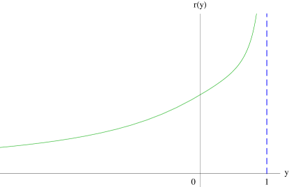
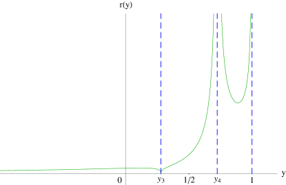
Let us begin with the case of high-power accretion (). Then, and, hence, we are in the region. Integration in Eq. (62) yields
| (67) | |||||
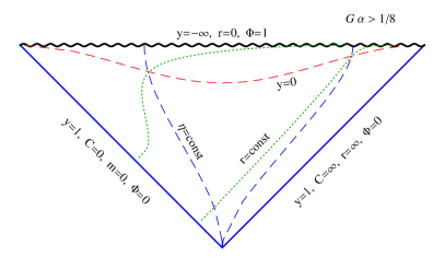
The behavior of function is qualitatively the same in the entire region (see Fig. 2). However, dependence behaves differently in the intervals , , and (see Figs. 2, 3). In accordance with expression (67), radius for is a monotonically increasing function of (from for to for ). We will refer to the case with as superpower accretion and the case with as simply strong accretion. It should also be noted that curves and are spacelike curves.
Apart from natural boundaries such as and infinities, the Carter-Penrose diagrams also display horizons of different types (zeroth, timelike, and spacelike), which represent the boundaries of diagrams; in this case, spherically symmetric spacetime consists of a certain set of triangles and squares separated by common boundaries. It should be noted that we have imposed additional physical requirement . As a result, physical spacetime may turn out to be geodetically incomplete.
Since by definition, our physical limitation leads to inequalities , , while implies that . Therefore, the boundaries are and . Everywhere, we have , i.e., the - region lies within the boundaries, where lines are spacelike ( plays the role of time, and this time increases from below), while the lines (or ) are timelike. Then, we see that boundaries () are spacelike and singular because invariant for .
At first glance, the boundaries for are zeroth boundaries. However, since and are in the denominator of and can vanish or turn to infinity, a more meticulous analysis is required. We will use two congruences of zeroth geodesics. Let us first consider incident beams for which . These beams begin from , where , , and enter the spacetime singularity . In can be seen that the boundary is indeed the zeroth infinity of past, where and . The value of along this boundary varies from to , while and .
The origin of the second boundary is more complicated. Let us consider the second congruence of zeroth geodesics for which . They begin from , where , , and for . Therefore, the boundary under investigation is a zeroth boundary, along which , , , and varies from to . Consequently, it is no longer infinite, but is the edge of zeroth beams that initiate accretion. This spacetime is obviously not geodetically complete (see Fig. 4). Analogous arguments for and lead to the diagrams shown in Figs. 5 and 6.
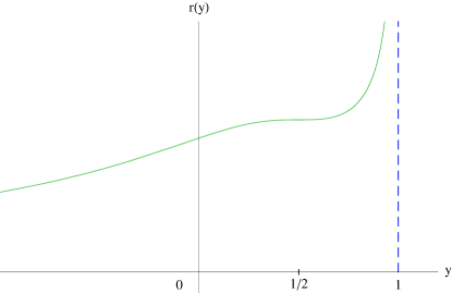
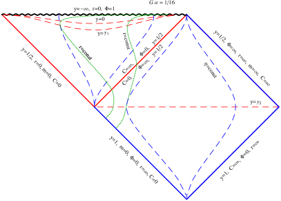
In the intermediate case of , function has the form
| (68) |
and
| (69) |
| (70) | |||||
(see Fig. 7). The Carter-Penrose diagram consists of two parts, viz., a triangle and a square joined together (and separated) by double horizon . Regions lie on both sides of this horizon, and lines are spacelike.
The triangle consists of spacelike singular lines, where , and two zeroth boundaries . One of these boundaries is a double horizon, while the other is a boundary zeroth beam with and . Operations with double horizons require carefulness because and . Let us consider the beams with , which produce accretion. It can be seen that for , and it is just the end of the range of coordinates in the triangle. For , we have , and it is the beginning of the new spatial range of coordinates in the square. For the boundary beam with , both and are equal to zero along . Invariant diverges, but point is a coordinate singularity (the determinant of the metric tensor is equal to zero at this point; see the description of the construction in Fig. 8).
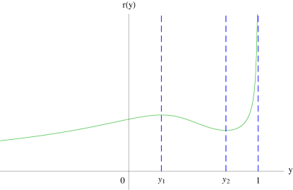
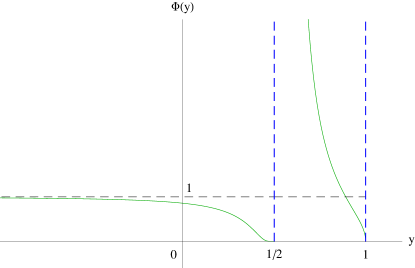
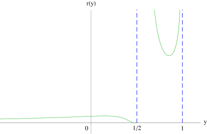
In the case of weak accretion (), the double horizon splits into two horizons for and . The new horizons appear due to the fact that, here, we are dealing with unbounded accretion with an infinite increase in the black hole mass. Function now assumes the form
| (71) |
and
| (72) |
| (73) |
(see the graphs in Fig. 9).
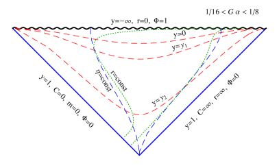
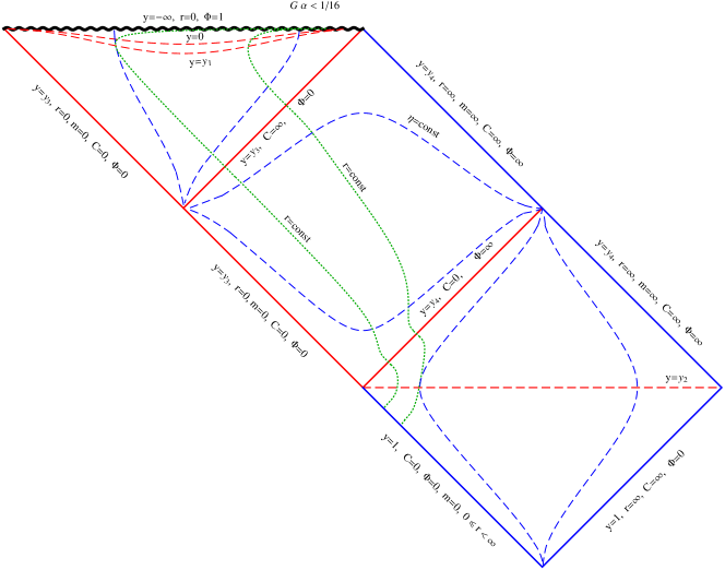
In this case, the global geometry is more complicated. The Carter-Penrose diagram consists of one triangle and two squares. The structure of the boundaries of the triangles remains the same as before (but now ), and we have the region in which the line is timelike, while is spacelike. The region also appears, the boundaries of which are new horizons and . The left boundary consists of two parts for . The latter is just the extreme zeroth beam of accretion with , , , and , while the upper boundary with and is an event horizon between the region and the region. The right boundary also consists of two parts for . The upper part of the boundary is the last accretion beam with , , , and (zeroth infinity of future), while the lower boundary is a cosmological horizon connecting the region and the outer region (). The second square () has the same structure except for the fact that now . As mentioned above, such spacetime is not geodetically complete (see the corresponding diagram in Fig. 10).
4 CONCLUSIONS
In this study, we have obtained the transformation of coordinates from the standard representation of the Vaidya metric with a linear mass function to two diagonal systems of coordinates and . The advantage of the linear model under investigation lies in the possibility of analytic calculation of all metric functions and light geodesics. It turns out that, in the presence of even weak accretion near the horizon, there is a narrow region in which the solution differs from the Schwarzschild solution not only quantitatively, but also qualitatively. Namely, apart from the visibility horizon, there are surfaces in diagonal coordinates with metric singularities and , which are surfaces of the infinite red and blue shifts, respectively. These surfaces serve as the boundaries of various coordinate systems, and their appearance distinguishes qualitatively the resultant metric of an accreting black hole from the Schwarzschild metric. It has been shown that one coordinate system with diagonal coordinates is insufficient for covering the entire spacetime; several such systems are required. The difference from the Schwarzschild metric (for example, in the case of very weak accretion) is associated with the divergence of coordinate time t for a radial light beam incident on the surface located outside the visibility horizon of a Vaidya black hole. In this case, the coordinate time of radially propagating photons on the visibility horizon turns out to be finite.
The divergence of the energy-momentum tensor components and on these surfaces is not associated with the presence of physical caustic, but is of purely coordinate origin. Indeed, analysis of the deviation equations for geodesics has shown that tidal forces are finite on surfaces and in the region (for ). For this reason, these surfaces are exclusively coordinate singularities, which can be referred to as false firewalls.
In the second set of diagonal coordinates , we have determined the maximal analytic continuation of the Vaidya metric in various cases that correspond to different accretion rates and have managed to construct a complete set of Carter-Penrose diagrams. These diagrams contain a set of spacetime regions separated by horizons and boundary lines (either or ), on which the operation of the coordinate systems terminates. The spacetime on the constructed diagrams is geodetically incomplete because we have imposed the physical condition of nonnegativity of mass function (); however, this construction is the maximum possible in the given physical formulation of the problem.
This study was supported by the Russian Foundation for Basic Research (project no. 15-02-05038-a).
References
- (1) P. C. Vaidya, Current Sci. 12, 183, (1943).
- (2) P. Vaidya, Proc. Indian Acad. Sci. A 33 264 (1951).
- (3) P. Vaidya, Nature 171, 260 (1953).
- (4) I. V. Volovich, V. A. Zagrebnov and V. P. Frolov, Theor. Math. Phys. 29, 1012 (1976).
- (5) W. A. Hiscock, Phys. Rev. D 23, 2823 (1981).
- (6) Y. Kuroda, Prog. Theor. Phys. 71, 1422 (1984).
- (7) M. I. Beciu, Phys. Lett. A 100, 77 (1984).
- (8) Y. Kaminaga, Class. Quantum Grav. 7, 1135 (1990).
- (9) Z. Zheng, C. Q. Yang and Q. A. Ren, Gen. Rel. Grav. 26, 1055 (1994).
- (10) A. N. St. J. Farley and P. D. D’Eath, Gen. Rel. Grav. 38, 425 (2006).
- (11) S. Sawayama, Phys. Rev. D 73, 064024 (2006).
- (12) H. Knutsen, Astron. Space Sci. 98, 207 (1984).
- (13) W. Barreto, Astron. Space Sci. 201, 191 (1993).
- (14) R. C. Adams, B. B. Cary and J. M. Cohen, Astron. Space Sci. 213, 205 (1994).
- (15) S. D. Maharaj, G. Govender and M. Govender, Gen. Rel. Grav. 44, 1089 (2012).
- (16) S. E. Hong, D. Hwang and E. D. Stewart and D. Yeom, Class. Quant. Grav. 27, 045014 (2010).
- (17) M. Alishahiha, A. F. Astaneh and M. R. M. Mozaffar, Phys. Rev. D 90, 046004 (2014).
- (18) W. A. Hiscock, L. G. Williams and D. M. Eardley, Phys. Rev. D 26, 751 (1982).
- (19) Y. Kuroda, Prog. Theor. Phys. 72, 63 (1984).
- (20) A. Papapetrou, A Random Walk in General Relativity, ed. J. Krishna-Rao, Wiley Eastern, New Delhi (1985), p 184.
- (21) B. Waugh and K. Lake, Phys. Lett. A 116, 154 (1986).
- (22) I. H. Dwivedi and P. S. Joshi, Class. Quantum Grav. 6, 1599 (1989).
- (23) I. H. Dwivedi and P. S. Joshi, Class. Quantum Grav. 8, 1339 (1991).
- (24) P. S. Joshi and I. H. Dwivedi, Gen. Rel. Grav. 24 129, (1992).
- (25) P. S. Joshi and I. H. Dwivedi, Phys. Rev. D 45, 2147 (1992).
- (26) P. S. Joshi and I. H. Dwivedi, Phys. Rev. D 47, 5357 (1993).
- (27) I. H. Dwivedi and P. S. Joshi, Commun. Math. Phys. 166, 117 (1994).
- (28) S. G. Ghosh and N. Dadhich, Phys. Rev. D 64, 047501 (2001).
- (29) M. D. Mkenyeleye, R. Goswami and S. D. Maharaj, Phys. Rev. D 90, 064034 (2014).
- (30) B. Waugh and K. Lake, Phys. Rev. D 34, 2978 (1986).
- (31) R. W. Lindquist, R. A. Schwartz, C. W. Misner, Physical Review 137, 1364 (1965).
- (32) O. Levin and A. Ori, Phys. Rev. D 54, 2746 (1996).
- (33) C.-G. Shao, B. Wang, E. Abdalla and R.-K. Su, Phys. Rev. D 71, 044003 (2005).
- (34) E. Abdalla and C. B. M. H. Chirenti, Phys. Rev. D 74, 084029 (2006).
- (35) I-C. Yang and C.-C. Jeng, Chin. J. Phys. 45, 497 (2006).
- (36) I. Bengtsson and J. M. M. Senovilla, Phys. Rev. D 79, 024027 (2009).
- (37) W. Israel, Phys. Lett. A 24, 184 (1967).
- (38) F. Fayos, M. M. Martín-Prats and J. M. M. Senovilla, Class. Quantum Grav. 12, 2565 (1995).
- (39) K. D. Krori and J. Barua, J. Phys. A: Math. Gen. 7, 2125 (1974).
- (40) B. Waugh and K. Lake, Phys. Rev. D 34, 2978 (1986).
- (41) V. A. Berezin, V. I. Dokuchaev, Yu. N. Eroshenko, Class. Quantum Grav. 33, 145003 (2016); arXiv:1603.00849 [gr-qc].
- (42) L. D. Landau and E. M. Lifshitz, The Classical Theory of Fields (Pergamon, Oxford, 1975).
- (43) K. A. Bronnikov and S. G. Rubin, Black Holes, Cosmology and Extra Dimensions (World Scientific, 2012).