$\theta$-parareal schemes

Abstract

A weighted version of the parareal method for parallel-in-time computation of time dependent problems is presented. Linear stability analysis for a scalar weighing strategy shows that the new scheme may enjoy favorable stability properties with marginal reduction in accuracy at worse. More complicated matrix-valued weights are analyzed and applied in numerical examples. The weights are optimized using information from past iterations, providing a systematic framework for using the parareal iterations as an approach to multiscale coupling. The advantage of the method is demonstrated using numerical examples, including some well-studied nonlinear Hamiltonian systems.

1 Introduction

Parallelization of computation for spatial domain, such as the standard domain decomposition methods, has been extensively developed and successfully applied to many important applications. Due to causality, parallel-in-time computations have not been as successful as parallel computations in space. However, numerical simulations will not benefit from available exa-scale computing power unless parallelization-in-time can be performed. Despite recent advances, the presence of strong causalities in the sense that local perturbations are not damped out by the system’s dissipation, e.g. in hyperbolic problems and fast oscillations in the solutions, typically hinders the efficiency of such types of algorithms. For example, approaches involving shooting and Newton’s solvers may become virtually unusable. It is widely recognized that robust and convergent numerical computation using such parallel-in-time algorithms still remains a main challenge.

Several attempts for designing time-parallel algorithms for evolutionary problems have been proposed. The common idea is to decompose the time domain of interest into several subintervals. In each subinterval, the given equation is solved in parallel with time-boundary conditions given at one or both ends of each subinterval. The time-boundary conditions are coupled via some specific algorithms, typically of iterative nature. With multiple shooting methods, see e.g. [12, 13], one solves a two-point boundary value problem in each subinterval, and uses a Newton’s iterations to couple all the boundary conditions together. Particularly for problems with oscillations, Newton iterations may not converge. A different approach, termed parareal, was proposed by Lions, Maday and Turinici in [15]. In the parareal framework, one solves an initial value problem in each subinterval with a high-accuracy “fine solver”, starting from the time-boundary conditions computed by a stable “coarse” solver. The coarse solution at the boundary of each subintervals is “corrected” iteratively by adding back the difference between the fine and the coarse solutions computed in the previous iteration. The standard parareal scheme was found to work quite well for dissipative problems. Loosely speaking, the parareal iterations typically converge quite well to the desired solution as long as it is stable.

In order to widen the range of applicability of parareal and increase its stability, several methods, combining parareal with other approaches, have been suggested. For example, Minion [16] proposes a “deferred spectral correction” scheme. Farhat and Chandesris [5] add a Newton-type iteration to reduce the jumps between the fine and coarse solutions. Gander et. al. [8] analyze the Krylov subspace approach of [5] for linear Ordinary Differential Equations (ODEs). The main idea is to use past iterations to form a subspace that can improve the coarse integrator. Although this method is applicable for low dimensional systems, it would become insufficient for high dimensional problems due to difficulties in orthogonalization in a large subspace. In [7], the authors manipulate the principle of superposition in linear ODEs to decouple inhomogeneous equations. Applying fast exponential integrators that are highly efficient for the homogenized part, the method is applicable to high-dimensional linear problems. Applications of parareal methods to Hamiltonian dynamics have been analyzed in [6]. Additional approaches applying symplectic integrators with applications to molecular dynamics include [2, 11]. Dai et. al. [3] proposed a symmetrized parareal version coupled with projections to the constant energy manifold.

In [14], a multiscale parareal scheme is proposed for dynamical systems possessing fast dissipative dynamics. It is found that the fast dissipative dynamics deteriorate the convergence of the “standard” parareal scheme, and suitable projections of the fast variables may improve the convergence property of such types of systems. In [1], a parareal like multiscale coupling schemes are proposed for highly oscillatory dynamical systems. In that work, the coarse integrator in the standard parareal scheme is replaced by a multiscale integrator that solves an effective system derived from the given highly oscillatory one. The coarse solutions are enhanced by an “alignment” process that uses the current fine solutions. The idea of aligning the fine and coarse solutions and propagating corrections on the coarse grid is also similar to the correction method proposed in [5]. Both of these approaches may be considered a special case of the general weighing scheme proposed in this paper. Several works have addressed the applicability of parareal methods to hyperbolic equations. It has been shown, that hyperbolic problems pose stability issues for parareal iterations, especially with large steps [4, 18, 5]. Applications include structural models [5], acoustic advection problems [17] and Partial Differential Equations (PDEs) with highly oscillatory forcing [10].

In this paper, we propose time-parallel algorithms motivated by the parareal methods of [15], due to its simple, derivative free, iterative structure. The main goal is to enhance the stability of the parareal iterations by taking a weighted linear combination of the previous and current iterations. The new method is termed $\theta$-parareal due to its formal resemblance to the known $\theta$-schemes for discretizing time dependent partial differential equations. Particular emphasis is given to oscillatory dynamical systems with essentially no dissipation. Furthermore, we provide a systematic approach for coupling computations involving different but in some sense “nearby” time dependent problems.

The paper is organized as follows. Section 2 presents our main approach and analyzes some of its important properties. Section 3 presents numerical examples. We conclude in section 4.

2 $\theta$-parareal

Consider ODEs of the form,

$$\frac{d}{dt}u=f(u),\>u(0)=u_{0}.$$

We are interested in a numerical approximation of the solution in a bounded time segment $[0,T]$. Throughout the paper it is assumed that solutions exist in $[0,T]$ and are sufficiently smooth.

Let $u_{n}^{(k)}\in\mathbb{C}^{d}$ denote the solution computed by the parareal schemes at iteration $k$ and time $t_{n}=nH.$ Let $F_{H}$ and $C_{H}$ denote the numerical propagators used as the fine (high accuracy but expansive) and coarse (low accuracy but cheap) integrators up to time $H$. The parareal scheme proposed in [15] is defined by the following simple iterations,

$$u_{n+1}^{(k+1)}=C_{H}u_{n}^{(k+1)}+\left(F_{H}u_{n}^{(k)}-C_{H}u_{n}^{(k)}\right),\,\,\,n,k=0,1,2,\dots,$$ (1)

with the initial conditions

$$u_{0}^{(k)}=u_{0},\,\,\,k=0,1,2,\dots.$$ (2)

The first (zero) iteration is taken as

$$u_{n+1}^{(0)}=C_{H}u_{n}^{(0)},\,\,\,n=0,1,2,\dots.$$

We shall refer to (1) as the standard parareal scheme.

Consider a weighted version of the parareal update,

$$u_{n+1}^{(k+1)}=\theta C_{H}u_{n}^{(k+1)}+(1-\theta)C_{H}u_{n}^{(k)}+\left(F_{H}u_{n}^{(k)}-C_{H}u_{n}^{(k)}\right),$$

leading to a more symmetric form,

$$u_{n+1}^{(k+1)}=\theta C_{H}u_{n}^{(k+1)}+\left(F_{H}u_{n}^{(k)}-\theta C_{H}u_{n}^{(k)}\right),$$ (3)

where $\theta$ are mappings from $\mathbb{C}^{d}$ to $\mathbb{C}^{d}$, which may depend on $k$ and $n$. In the general case, the weights $\theta$ will be denoted $\theta_{n}^{(k)}$, i.e.,

$$u_{n+1}^{(k+1)}=\theta_{n+1}^{(k+1)}C_{H}u_{n}^{(k+1)}+\left(F_{H}u_{n}^{(k)}-\theta_{n+1}^{(k+1)}C_{H}u_{n}^{(k)}\right).$$ (4)

We start with the simplest case where $\theta$ is a real number, then a complex number and finally linear operators. We note that the method can still be parallelized as the initial condition for the fine integrator only depends on the previous iteration. We view $\theta C_{H}$ as a new coarse integrator, and investigate in what (simple) ways $\theta$ can enhance stability and accuracy of the original parareal ($\theta\equiv 1$).

We shall first show that the new schemes preserve the “exact causal property” as the original parareal scheme, i.e., that, given in $H$, the method will always converge to the fine solutions $(F_{H})^{n}u_{0}$ after $T/H$ iterations. Indeed, we notice that if $u_{n}^{(k)}=u_{n}^{(k+1)},$ then the recurrence relations in (1) or (3) reduce to advancing from $t_{n}$ to $t_{n}+H$ using the fine scale integrator, i.e., $u_{n}^{(k)}=(F_{H})^{n}u_{0}$ is a fixed point. More precisely, given the initial condition (2) we see that

$$u_{1}^{(1)}=\theta_{1}^{(1)}C_{H}u_{0}+(F_{H}u_{0}-\theta_{1}^{(1)}C_{H}u_{0})=F_{H}u_{0},$$

and

$$u_{1}^{(k)}=\theta_{1}^{(k)}C_{H}u_{0}^{(k)}+(F_{H}u_{0}^{(k-1)}-\theta_{1}^{(k)}C_{H}u_{0}^{(k-1)})=F_{H}u_{0},k=1,2,\dots.$$

By induction,

$$u_{j}^{(k+1)}=(F_{H})^{j}u_{0},\,\,\,j\leq k,$$

which implies that,

$$u_{k+1}^{(k+1)} =\theta_{k+1}^{(k+1)}C_{H}u_{k}^{(k+1)}+(F_{H}u_{k}^{(k)}-\theta_{k+1}^{(k+1)}C_{H}u_{k}^{(k)})=(F_{H})^{k+1}u_{0},\,\,\,k=0,1,2,\dots.$$

Hence, we have the following exact causality property:

Theorem 2.1.

Let $u_{n}^{(k)}$ solve (1) and (2). Then,

$$u_{n}^{(k)}=(F_{H})^{n}u_{0},\,\,\,\,\forall k\geq n.$$

The surprising thing about this result is that it holds even if the effective coarse integrator $\theta C_{H}$ is not consistent with the ODE.

We now consider a simple case in which $\theta,$ $C_{H}$ and $F_{H}$ are linear operators, independent of $n$ and $k$. In order to study the stability and convergence of the $\theta$-scheme, let $v_{n+1}^{(k)}$ denote the correction term $F_{H}u_{n}^{(k)}-\theta C_{H}u_{n}^{(k)}$. Then $\theta$-parareal can be written as,

$$u_{n+1}^{k+1} = \theta C_{H}u_{n}^{(k+1)}+v_{n+1}^{(k)}$$

$$= (\theta C_{H}\circ\theta C_{H})u_{n-1}^{(k+1)}+\theta C_{H}v_{n}^{(k)}+v_{n+1}^{(k)}$$

$$\vdots$$

$$= (\theta C_{H})^{n+1}u_{0}^{(k+1)}+\sum_{j=1}^{n+1}\left(\prod_{i=j+1}^{n+1}\theta C_{H}\right)v_{j}^{(k)}.$$

Here we use the notation,

$$(\theta C_{H})^{\ell}u=(\prod_{j=1}^{\ell}\theta C_{H})u=\underbrace{\theta C_{H}\circ\theta C_{H}\cdots\theta C_{H}}_{\ell\text{ times}}u.$$

For a fixed $k$, the stability of the time marching is determined by $(\theta C_{H})^{n}$. Having a stable coarse solver is crucial in stabilizing the parareal solution because the correction is often small up to the order of accuracy. However, it will be interesting to consider examples in which, introducing the factor $\theta$ can stabilize iterations. Suppose one runs the parareal scheme in a time interval consisting of $N$ coarse sub-intervals. Define, $U^{(k)}:=(u_{0}^{(k)},u_{1}^{(k)},\cdots,u_{N}^{(k)})^{T},$ $I_{0}=\left(u_{0},0,\ldots,0\right)^{T}$, and

$$A=\left(\begin{array}[]{ccccc}I&0&\ldots&0&0\\ -\theta C_{H}&I&\ldots&0&0\\ 0&-\theta C_{H}&\ddots&0&0\\ \vdots&\vdots&\ddots&\vdots&\vdots\\ 0&0&\ldots&-\theta C_{H}&I\end{array}\right),B=\left(\begin{array}[]{ccccc}0&0&\ldots&0&0\\ F_{H}-\theta C_{H}&0&\ldots&0&0\\ 0&F_{H}-\theta C_{H}&\ddots&0&0\\ \vdots&\vdots&\ddots&\vdots&\vdots\\ 0&0&\ldots&F-\theta C_{H}&0\end{array}\right).$$

Then, the $\theta$-parareal iteration can be written in matrix form as,

$$AU^{(k+1)}=BU^{(k)}+I_{0},$$

with initial condition $U^{(0)}=(u_{0},C_{H}u_{0},\cdots,(C_{H})^{N}u_{0}).$ Thus, we obtain an explicit expression of $U^{(k)}$,

$$U^{(k+1)}=A^{-1}BU^{(k)}+A^{-1}I_{0}.$$

We readily see that $U^{*}=(u_{0},F_{H}u_{0},\cdots,(F_{H})^{N}u_{0})$ is a fixed point, $U^{*}=A^{-1}BU^{*}+A^{-1}I_{0}$. Denoting the signed error $E_{n}^{(k)}=U^{(k)}-U^{*},$ it is given by,

$$E^{(k+1)}=A^{-1}BE^{(k)}=\left(\begin{array}[]{cccccc}0\\ I&0\\ \theta C_{H}&I&0\\ (\theta C_{H})^{2}&\ddots&\ddots&\ddots\\ \vdots&\ddots&C_{H}&I&0\\ (\theta C_{H})^{N-1}&\cdots&(\theta C_{H})^{2}&\theta C_{H}&I&0\end{array}\right)(F_{H}-\theta C_{H})E^{(k)},$$

where $E^{(0)}=(0,(F_{H}-C_{H})u_{0},(F_{H}^{2}-C_{H}^{2})u_{0},\cdots,(F_{H}^{N}-C_{H}^{N})u_{0})^{T}$. We find the following theorem.

Theorem 2.2.

Let $e_{n}^{(k)}:=u_{n}^{(k)}-(F_{H})^{n}u_{0},$ $n=0,1,\cdots,N,$ and $k\leq n.$ The following inequality holds,

$$|e_{n}^{(k+1)}|\leq\|F_{H}-\theta C_{H}\|_{\infty}\sum_{j=0}^{n-k-2}\|\theta C_{H}\|_{\infty}^{j}\,|e_{n}^{(k)}|.$$ (5)

Note that this estimate can be derived from Theorem 4.5 in [9] by formally replacing $C_{H}$ with $\theta C_{H}$ and $F_{H}$ with the exact solution operator that advances the solution by a time length $H$. Nonetheless, the difference is important for the discussion below and provides insight into how a parareal method would perform, depending on the stability of $F_{H}$, $C_{H}$, $N$, and the accuracy of $C_{H}$. We would like to see under what conditions the parareal iterations decrease the errors. This translates to finding conditions that render the amplification factor $Q_{n,k}:=|F_{H}-\theta C_{H}|\sum_{j=0}^{n-k-2}|\theta C_{H}|^{j}<1.$ We immediately see that a deciding factor is whether $\sum_{j=0}^{n-k-2}|\theta C_{H}|^{j}$ is uniformly bounded in $n$.

Theorem 2.3.

(nonlinear variable coefficient case) Let $e_{n}^{(k)}:=u_{n}^{(k)}-(F_{H})^{n}u_{0},$ $n=0,1,\cdots,N,$ and $k\leq n.$ Then $u_{n}^{(k)}$ is given by,

$$u_{n+1}^{k+1}=\left[\prod_{j=1}^{n+1}\theta_{j}^{(k)}C_{H}\right]u_{0}^{k+1}+\sum_{j=1}^{n+1}\left[\prod_{i=j+1}^{n+1}\theta_{i}^{(k)}C_{H}\right](F_{H}u_{j-1}^{k}-\theta_{j-1}^{(k)}C_{H}u_{j-1}^{k}).$$

Furthermore, the following inequality holds,

$$|e_{n}^{(k+1)}|\leq\|F_{H}-\theta C_{H}\|_{\infty}\sum_{j=0}^{n-k-2}\|\theta C_{H}\|_{\infty}^{j}\,|e_{n}^{(k)}|.$$ (6)

The proof is similar to the linear case. We see that the solution is composed of coarse solution and a series of propagating correction.

2.1 Linear theory

We consider a diagonalizable linear system of first order differential equations,

$$\frac{d}{dt}U=AU,\,\,\,U(t)\in\mathbb{R}^{d},$$ (7)

where the $d\times d$ complex matrix $A$ can be diagonalized, $A=P\Lambda P^{-1}$ and $\Lambda=\text{diag}(\lambda_{1},\cdots,\lambda_{d})$. By a change of variable $U\mapsto P^{-1}U$, the system is decoupled into $d$ linear scalar equations on the complex plane. Consequently, the system obtained by applying a typical linear numerical integrator can be diagonalized in the same fashion. We consider using standard one-step linear integrators as our choice of $F_{H}$ and $C_{H}$. Therefore, $F_{H}u$ and $C_{H}u$ simply multiply $u$ by suitable complex numbers. In addition, we will consider $\theta\in\mathbb{C}$, which obviously commutes with $P$ and $P^{-1}.$ Overall, in this section we consider initial value problems of the model scalar equation,

$$u^{\prime} =\lambda u,\,\,\,\lambda\in\mathbb{C},$$ (8)

$$u(0) =u_{0}.$$

Dissipation helps.

Here, by dissipation, we mean that all eigenvalues of $A$ have negative real parts. We start by analyzing the standard parareal $(\theta=1)$. For problems with dissipation, stable and consistent solvers will naturally have an amplification factors that is strictly less than one. Suppose that the coarse solver is strictly stable in the sense that $|C_{H}|\leq r_{0}<1,$

$$1<\sum_{j=0}^{m-1}|C_{H}|^{j}=\frac{1-r_{0}^{m}}{1-r_{0}}<\frac{1}{1-r_{0}}.$$

Assume that $F_{H}$ and $C_{H}$ are consistent with the same equation, that $F_{H}$ is $p$-th order method with step size $h\ll H$, and $C_{H}$ is a $q$-th order method with step size $H$. For $u_{0}$ in a compact subset of the complex plane,

$$|F_{H}u_{0}-C_{H}u_{0}|\leq K_{1}e^{Re[\lambda H]}h^{p}+K_{2}H^{q+1},$$

where $K_{1}$ and $K_{2}$ are two constants that depend on $\lambda$, the solvers, $h$ and $H$. As a result, the stability of a standard parareal ($\theta=1$) for $k<n\leq N$ requires that,

$$K_{1}e^{|\lambda|H}h^{p}+K_{2}H^{q+1}<1-r_{0}.$$

If Re$\lambda<0$, then the terms on the Left Hand Side (LHS) are bounded in time and the inequality holds for sufficiently small step sizes. However, with oscillatory problems ($\lambda$ purely imaginary), the exponential terms may prohibit a large ratio of $H/h$, which limits the attractiveness of the parareal approach.

Next, we define the amplification factor, which is an upper bound on the grows of the parareal error.

$$Q_{N^{\prime},k}=|F_{H}-\theta C_{H}|\sum_{j=0}^{N^{\prime}-k-2}|\theta C_{H}|^{j}.$$

Comparing with the the error bounds (6), it is clear that the parareal iteration will not be stable unless $Q_{N^{\prime},k}<1$. We make several observations regarding this bound.

• The parareal iteration can produce solutions that converge globally to the one computed by the fine solver, even if $F_{H}$ and $C_{H}$ do not solve the same equation. The iterations will converge as long as (i) the coarse solver is strictly stable, i.e. $|C_{H}|\leq r_{0}<1$, and (ii) the gap between the fine solver and the coarse solver is sufficiently small; i.e. $|F_{H}u_{0}-C_{H}u_{0}|<1-r_{0}.$ One simple way to guaranty that is to choose a coarse solver that can at least approximately propagate the causality of the given problem.

• The above estimates and observations apply when we formally replace $C_{H}$ by $\theta C_{H}.$

• If the problem is dissipative, then $|C_{H}|<1$, and parareal is stable as long as $C_{H}$ (or $\theta C_{H}$) are sufficiently close. However, in general, there exists a maximal value of coarse steps, $N^{{}^{\prime}}$, that depends on inverse powers of $H$ ($h<H$) such that for $n<N^{\prime}$ the errors $|e_{n}^{(k)}|$ decreases as $k$ increases, while for $n\geq N^{\prime}$, the error $|e_{n}^{(k)}|$ grows exponentially as $k$ increases. For example, if $\theta=1,$ $|C_{H}|=1,$ $k=1$, then we need to pick an $N^{\prime}$ such that i.e.,

  $$Q_{N^{\prime},1}\leq K_{3}H^{q+1}N^{\prime}<1.$$

  Note that this estimate is note sharp. See, for example, Gander and Hairer [6] provide sharp bounds for the number of allowed steps in solving Hamiltonian systems using symplectic integrators.

Purely oscillatory problems are more challenging.

We focus our discussion around the typical case when the coarse solver is border-line stable; i.e. $|C_{H}|=1$ and $0<\delta\leq|F_{H}|\leq 1$, where $\delta$ is a lower bound of $|F_{H}|$. A significant implication is that the parareal iterations will become unstable after several coarse steps because $\sum_{j=0}^{N-k-2}|C_{H}|^{j}=N-k-1$. In this case, we see that stability can be gained by multiplying $C_{H}$ by a factor $\theta$. In the extreme case of $\theta=0,$ the errors in the parareal iterations trivially satisfy,

$$|e_{n}^{(k+1)}|\leq|F_{H}|\,|e_{n}^{(k)}|.$$

The errors do not necessarily decrease (for $n>k$), unless $|F_{H}|<1;$ i.e. unless the fine solver is strictly linearly stable. For the case $0<\theta<1$,

$$1<\sum_{j=0}^{N-k-2}|\theta C_{H}|^{j}=\frac{1-\theta^{N-k-2}}{1-\theta}<\frac{1}{1-\theta}.$$

The amplification factor is thus bounded by

$$Q_{n,k} \leq|F_{H}-\theta C_{H}|\sum_{j=0}^{n-k-2}|\theta C_{H}|^{j}$$

$$\leq\min\left\{|F_{H}|+\theta,\left(K_{1}h^{p}+K_{2}H^{q+1}+(1-\theta)\right)\right\}\frac{1-\theta^{N-k-2}}{1-\theta},$$

The term $K_{1}h^{p}H+K_{2}H^{q+1}$ come from the local errors of $F_{H}$ and $C_{H}$. When $K_{1}$ and $K_{2}$ are reasonably small, i.e., the numerical schemes resolves the solution of the differential equation with sufficiently high accuracy, $Q_{n,k}$ is minimized for $\theta=1$. However, if the coarse solver does not resolve the differential equation well, then $K_{2}$ can be very large. This is the case if $C_{H}$ is some multiscale solver which solves a different differential equation, or when there are Dirac$\delta$-like impulses in the system. In such a case, it is reasonable to assume that

$$|F_{H}|+\theta<K_{1}h^{p}+K_{2}H^{q+1}+(1-\theta).$$ (9)

In this case, using an appropriate value of $\theta$ may stabilize the parareal iterations. For example, one may take a $\theta$ that falls into the range,

$$(|F_{H}|+\theta)\frac{1}{1-\theta}<1,\,\,\,i.e.,\,\,\,0\leq\theta<\frac{1-|F_{H}|}{2}.$$

Again, we see that it is necessary to have $|F_{H}|<1;$ i.e., if $\theta$ is taken to be a real number then some dissipation in the fine solver is necessary for stability .

In the more challenging cases in which $|C_{H}|=1$ and $|F_{H}|=1$, the parareal iterations needs to be stabilized in another way. We first look at the following motivating example.

Example 2.4.

We consider using the A-stable Trapezoidal rule as both the coarse and fine integrators, $C_{H}=(1+\lambda H/2)/(1-\lambda H/2)$ and $F_{H}=\left((1+\lambda h/2)/(1-\lambda H/2)\right)^{H/h}.$ Let $\lambda=-3$ and $H=1$, so that $|C_{H}|=1/5$ and

$$\sum_{j=0}^{m-1}|C_{H}|^{j}=\frac{5}{4}(1-\frac{1}{5^{N}})<\frac{5}{4}$$

is bounded independent of $N.$ It is clear that parareal iterations easily converge in this case. Next, consider the oscillatory case with $\lambda=3i$ and $H=1.$ Now, we have $|C_{H}|=|F_{H}|=1$ and

$$\sum_{j=0}^{m-1}|C_{H}|^{j}=m.$$

We see that the standard parareal algorithm performs poorly compared to the dissipative case. However, since $C_{H}=(-5+12i)/13$, it is possible to multiply $C_{H}$ by a complex constant $\theta=re^{i\phi_{H}}$ to minimize the difference $F_{H}u-\theta C_{H}$. For example, taking $h=H/20$, $F_{H}=(1591+240i)/1609$ and $\theta=F_{H}/C_{H}\approx-0.24-0.97i$ will drastically improve the convergence and stability of the scheme. The interpretation is that multiplication by $\theta$ rotates the coarse solution $C_{H}u$ to have a similar phase as $F_{H}u$. This is a direct analogy to the “phase alignment” procedure proposed in [1].

In fact, following the old idea of of linear stability of a scheme for ordinary differential equations, one can systematically look at the stability property of a “$\theta$-parareal” scheme, for $\theta\in\mathbb{C}$,

Definition 2.5.

(Region of parareal-stability) For each $N>0$ and $\xi_{0}\in\mathbb{C}$, define the set

$$\mathcal{R}_{\{\lambda H=\xi_{0}\}}^{N}:=\{\theta\in\mathbb{C}:|F_{H}-\theta C_{H}|\sum_{j=0}^{N-2}|\theta C_{H}|^{j}\leq 1\}.$$ (10)

We shall refer to $\mathcal{R}_{\{\lambda H=\xi_{0}\}}^{N}$ as the region of parareal-stability for the model equation (8). Taking $\theta\in\mathcal{R}_{\{\lambda H=\xi_{0}\}}^{N}$ in (3) for solving (8), guaranties that the resulting errors $|e_{j}^{(k)}|$ will decrease to $0$ as $k$ increases for all $0\leq j\leq N$ .

Figures 1 and 2 show a few examples of the regions of parareal-stability of different choices $C_{H}$, $F_{H}$, and $H$. We see that for large $|\lambda H|$, stabilization of the parareal scheme may require $\theta$ to have non-zero imaginary part; i.e., the coarse solutions need to be rotated.

We have seen that, particularly for problems involving oscillations, the deciding factor for stability and performance of parareal iterations lies in how well $C_{H}$ approximates $F_{H}$. For oscillatory problems and “marginally stable” integrators, for example in system that preserve certain energy or invariance, it is necessary to bridge the gap between the coarse and fine integrators by suitable rotations. Figure 3 shows the amplification factors $Q_{n,0}$ of the standard parareal method involving Forward and backward Euler schemes and the corresponding cases for the $\theta$-parareal scheme, with $\theta$ in $\mathcal{R}_{\{\lambda H=0.1i\}}^{N}$. The results demonstrate that when the number of step is large ($N=10^{4}$ in simulations), stability becomes a critical issue.

Summarizing this example, it is our objective to choose an optimized choice of $\theta$ to achieve $|F_{H}-\theta C_{H}|\ll|F_{H}-C_{H}|$ while keeping $\sum_{j=0}^{N}|\theta C_{H}|^{j}$ to a moderate size for some $N$. $\theta C_{H}$ can be viewed as an improved coarse solver. In the next section, we present two strategies for achieving this objective.

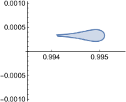
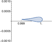
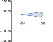
Figure 1: Oscillatory example: The region of parareal-stability for (left) forward Euler, (center) trapezoidal rule and (right) backward Euler as both the fine and coarse integrators. Parameters are $\lambda H=0.1i$ and $N=10^{4}$. Note that $\theta=1$ is not always included in the stability region.

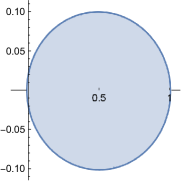
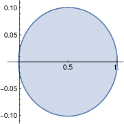
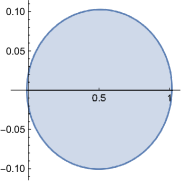
Figure 2: Dissipative example: The region of parareal-stability for (left) forward Euler, (center) trapezoidal rule and (right) backward Euler as both the fine and coarse integrators. Parameters are $\lambda H=-0.02+0.1i$ and $N=10^{4}$. Note that $\theta=1$ is included in the stability region, as expected for dissipative systems.

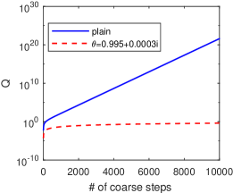
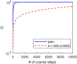
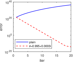
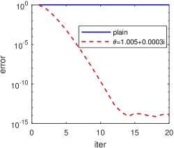
Figure 3: Convergence of the parareal iterations for a scalar linear ODE. Top row: The amplification factor $Q_{m,0}=|F_{H}-\theta C_{H}|\sum_{j=0}^{m-2}|\theta C_{H}|^{j}$. Bottom row shows the computed errors with parameters $\lambda H=0.1i$ and $N=10^{4}$. $F_{H}$ is taken to be the exact solution operator. The left column shows the results from $C_{H}$ being forward Euler scheme, and the right column the implicit Euler.

2.2 “Sequentializing” parareal

Let $a=|F_{H}-\theta C_{H}|$ and, for oscillatory problems, $b=\sum|\theta C_{H}|^{j}=N-k-2.$ Assuming a coarse solver with step size $H$ and order $q$, $a\sim H^{q+1}$, which implies, following the stability analysis, that $N<H^{-(q+1)}$. Therefore, we should not run parareal for more than $N\sim H^{-(q+1)}$ time steps.

In order to overcome this limitation, we propose the divide the the time interval of interest $[0,T]$ to $s$ subintervals of equal length and preform parareal sequentially. A similar idea has been suggested in [6]. As we describe below, this does not significantly reduce the computational cost for moderate values of $s$.

Computational cost

Assume that the coarse and fine integrators apply numerical schemes using step sizes $H$ and $h$, respectively. Let $n_{CPU}$ denote the number of CPUs available and assume that $n_{CPU}<T/H$ . Then, the computational cost of $K$ standard parareal iterations consists of coarse solver, fine solver operations and extra cost for data transfer between processors

$$C_{p}=K\left(\dfrac{T}{H}+\dfrac{T}{n_{CPU}h}+c_{com}\right)$$

where $c_{com}$ is the cost of communication. Sequential parareal processes a shorter time interval at once, $t=T/s$. Then, assuming that $n_{CPU}<T/(Hs)$, the computational cost of sequential parareal is,

$$C_{sp}=sK\left(\dfrac{T}{Hs}+\dfrac{T}{n_{CPU}hs}+c_{com}\right)\backsimeq C_{p}+sKc_{com}.$$

Therefore, if the number of processors is not very large (compared to the maximal theoretical gain using parareal, $T/H$ ) and the communication in a parallel cluster is efficient, then the computational cost of sequential parareal is comparable to standard parareal.

2.3 Optimized choices of $\theta$

Formula (3) and the error estimate (6) suggest that $\theta$ needs to bring the coarse scheme to be closer to the fine one. Indeed, if we can find, without a significant computational overhead, an operator $\theta$ such that $\theta C_{H}u\equiv F_{H}u$ for all $u\in\mathbb{R}^{d}$, then the parareal scheme is reduced to simply

$$u_{n+1}^{(k+1)}=\theta C_{H}u_{n}^{(k+1)}\equiv F_{H}u_{n}^{(k+1)}.$$ (11)

This means that we shall enjoy the accuracy of the fine integrator.

In practice, it is more reasonable to approximate $F_{H}u_{n}^{(k+1)}$ point-wise, using the data gathered from the evaluations of $F_{H}$ at previously computed points $\{u_{n}^{(k)}\}$. Accordingly, we shall use the notation $\theta_{n}^{(k)}C_{H}$ to be the approximation defined near $u_{n}^{(k+1)}$. Of course, the idea of “recycling” the computed data to improve the coarse solver is not new. Some existing parareal algorithms that apply similar approaches have been suggested and analyzed in [5] and [18]. The point of view of this paper is different as our focus is on increasing the stability of iterations, even at the cost of high-order accuracy.

Given a choice of coarse and fine integrators, we assume the $\theta_{n}^{(k)}$ is an operator that acts on all previous coarse points $\{u_{n}^{(j)}\}_{j=0}^{k}$ into the states space. For simplicity, we will restrict the discussion to affine linear maps, denoted $\Theta:\mathbb{R}^{d\times(k+1)}\to\mathbb{R}^{d}$ . We consider two approaches in construction of $\theta_{n}^{(k)}$. The first is a variational approach which directly attempt to minimize the mismatch between the fine and coarse integrators over a suitable set of points $\Omega_{n}^{(k)}$ that includes $\{u_{n}^{(j)}\}_{j=0}^{k}$ and possibly additional points in its vicinity,

$$\theta_{n}^{(k)}=\arg_{\theta\in\Theta}\text{$\min$}{}_{u\in\Omega_{n}^{(k)}}||F_{H}u-\theta C_{H}u||,$$ (12)

where $||\cdot||$ can be the operator or other suitable norm. In particular, if $C_{H}$ is invertible, then we may simply take

$$\theta_{n}^{(k)}\equiv F_{H}C_{H}^{-1}.$$

We remark that while such approaches may be doable for smaller systems, it is not practical for large systems unless some low-rank approximation of $F_{H}$ can be computed efficiently in $\Omega_{n}^{(k)}$.

Interpolation

Assuming that $\theta$ is affine and that $\Omega_{n}^{(k)}$ is a finite set, then the minimization (12) can be obtained using linear interpolation. Here, we consider the case where, $k\geq d$, the set $\Omega_{n}^{(k)}$ includes the last $d+1$ parareal approximations for the $n$’th coarse step, $\Omega_{n}^{(k)}=\left\{u_{n}^{(k-d)},\dots,u_{n}^{(k)}\right\}$. Hence, the linear operator $\theta:\mathbb{R}^{d\times(k+1)}\to\mathbb{R}^{d}$ satisfies

$$\theta_{n}^{(k)}C_{H}(u_{n}^{(k-j)})=F_{H}u_{n}^{(k-j)},\,\,\,j=0\dots d,$$ (13)

In the next section, we shall present some numerical simulations using the following construction

$$\theta_{n}^{(k)}C_{H}(w):=C_{H}w+I_{n}^{(k)}(w;\{u_{n}^{(k-j)}\}_{j=0}^{d}),$$ (14)

where $I_{n}^{(k)}(w;\Omega_{n}^{(k)})$ are affine approximations of the function $\kappa(u):\mathbb{R}^{d}\to\mathbb{R}^{d},$

$$\kappa(u):=\left[F_{H}-C_{H}\right]u,$$

which linearly interpolate the points in a set $\Omega_{n}^{(k)}$; i.e.

$$I_{n}^{(k)}(u_{n}^{(k-j)};\{u_{n}^{(k-j)}\}_{j=0}^{d})=\kappa(u_{n}^{(k-j)})=\left[F_{H}-C_{H}\right]u_{n}^{(k-j)},\,\,\,j=0\dots d.$$ (15)

For brevity, we shall write below $I_{n}^{(k)}w=I_{n}^{(k)}(w;\{u_{n}^{(k-j)}\}_{j=0}^{d})$. Using, (14) and (15),

$$\theta_{n}^{(k)}C_{H}u_{n}^{(k)}=C_{H}u_{n}^{(k)}+I_{n}^{(k)}u_{n}^{(k)}=C_{H}u_{n}^{(k)}+\left[F_{H}-C_{H}\right]u_{n}^{(k)}=F_{H}u_{n}^{(k)}.$$

Substituting into the$\theta$-parareal update,

$$u_{n+1}^{(k+1)}=\theta_{n}^{(k)}C_{H}u_{n}^{(k+1)}+F_{H}u_{n}^{(k)}-\theta_{n}^{(k)}C_{H}u_{n}^{(k)}=\theta_{n}^{(k)}C_{H}u_{n}^{(k+1)}=\left[C_{H}+I_{n}^{(k)}\right]u_{n}^{(k+1)}.$$ (16)

2.3.1 Error estimates

Let us consider the interpolative approach from the view point of a linear approximation of the function $\kappa(u).$ An “ideal” parareal update (11), in the sense that $u_{n}^{(k)}=F_{H}^{n}u_{0}$, could be written as

$$u_{n+1}^{(k+1)}=C_{H}u_{n}^{(k+1)}+\kappa(u_{n}^{(k+1)}).$$ (17)

However, $\kappa(u_{n}^{(k+1)})$ are not known and need to be approximated. In this formulation, standard parareal amounts to approximating $\kappa(u_{n}^{(k+1)})$ by $\kappa(u_{n}^{(k)})$. We may make use of Taylor series to design higher order approximation of $\kappa$ near the computed values. Expanding $\kappa$ around $u_{n}^{(k)},$we have

$$\kappa(w)=\kappa(u_{n}^{(k)})+D_{\kappa}(u_{n}^{(k)})(w-u_{n}^{(k)})+R_{2}(w-u_{n}^{(k)}),$$ (18)

where $R_{2}$ is the second order (in the sense of small distance to $u_{n}^{(k)})$ remainder term. In this way, the “ideal” parareal update then formally becomes,

$$u_{n+1}^{(k+1)}=C_{H}u_{n}^{(k+1)}+\kappa(u_{n}^{(k)})+D_{\kappa}(u_{n}^{(k)})(u_{n}^{(k+1)}-u_{n}^{(k)})+R_{2}(u_{n}^{(k+1)}-u_{n}^{(k)}).$$ (19)

We may define a parareal update by truncating the higher order terms, $R_{2}$ in the expansion of $\kappa$ around $u_{n}^{(k)}$. The following Lemma shows that $\kappa(u_{n}^{(k)})+D_{\kappa}(u_{n}^{(k)})(w-u_{n}^{(k)})$ can be approximated to second order by linear interpolation.

Lemma 2.6.

Let $x\in\mathbb{R}^{d}$ and let $\Omega=\left\{x_{0},\dots,x_{d}\right\}\subset\mathbb{R}^{d}$ be a set of $d+1$ interpolation points in $B_{\epsilon}(x)=\left\{w:\left|w-x\right|<\epsilon\right\}$ for some $\epsilon>0$. Let

$$V=\left[\begin{array}[]{cccc}x_{0}&\;x_{1}&\;\cdots&\;x_{d}\\ 1&1&\;\cdots&\;1\end{array}\right],$$

a $(d+1)\times(d+1)$ matrix, and assume that $\det V\neq 0$. Let $\kappa:\mathbb{R}^{d}\to\mathbb{R}^{d}$ denote a $C^{2}$ function in the $\epsilon$-ball. Let $l:\mathbb{R}^{d}\to\mathbb{R}^{d}$ denote the unique affine function, $l(w)=l_{0}+Aw$, such that $\kappa(w)=l(w)$ for all $w=x_{0}\dots x_{d}$. Then,

$$\left|\kappa(x)-l(x)\right|\leq C\frac{\epsilon^{2}}{\sigma_{\min}},$$

for some constant $C>0$, where $\sigma_{\min}$ is the smallest singular value of $V$.

Proof.

Without loss of generality, we take $x=0$. Denote

$$l(w)=L\left[\begin{array}[]{c}w\\ 1\end{array}\right],$$

where $L$ is a $d\times(d+1)$ matrix that satisfies

$$LV=F=\left[\kappa(x_{0})\;\cdots\;\kappa(x_{d})\right].$$

Since $V$ is invertible, $L:=FV^{-1}$ is uniquely defined. Also, expanding $\kappa$ in a Taylor series around $0$ and evaluating at $x_{j},$

$$\kappa(x_{j})=\kappa(0)+\nabla\kappa(0)x_{j}+O(\epsilon^{2}),$$

or, arranging these $d+1$ columns in a matrix,

$$F=\kappa(0)\left[1\;\cdots\;1\right]+\nabla\kappa(0)\left[x_{0}\;\cdots\;x_{d}\right]+O(\epsilon^{2})=\left[\nabla\kappa(0)\;\kappa(0)\right]V+O(\epsilon^{2}).$$

Multiplying by $V^{-1}$ we conclude that $L=\left[\nabla\kappa(0)\;\kappa(0)\right]+O(\epsilon^{2}/\sigma_{\min})$. As a result,

$$l(0)=\left[\nabla\kappa(0)\;\kappa(0)\right]\left[\begin{array}[]{c}0\\ \vdots\\ 0\\ 1\end{array}\right]+O(\epsilon^{2}/\sigma_{\min})=\kappa(0)+O(\epsilon^{2}/\sigma_{\min}),$$

which proves the Lemma. ∎

Returning to interpolative $\theta$-parareal, we take $x_{j}=u_{n}^{(k-j)}$. Assume that, at time step $n$, parareal reached accuracy $\epsilon$ in the last $d+1$ iterations, i.e.,

$$\max_{j=0\dots d}|u_{n}^{(k-j)}-F_{H}^{n}u_{0}|<\epsilon.$$

Then, using Lemma 2.6 with $x=u_{n}^{(k+1)}$, the linear interpolation $I_{n}^{(k)}(w;\left\{u_{n}^{(k+1)}\right\}_{j=0}^{d})$ satisfies,

$$I_{n}^{(k)}u_{n}^{(k+1)}=\kappa(u_{n}^{(k+1)})+O(\epsilon^{2}/\sigma_{\min}).$$

Using (17) implies that

$$|u_{n+1}^{(k+1)}-F_{H}^{n+1}u_{0}|=O(\epsilon^{2}/\sigma_{\min}).$$ (20)

We conclude that, after every $d+1$ iterations of the interpolative $\theta$-parareal, the error $\epsilon$ is reduced to $O(\epsilon^{2}/\sigma_{\min})$. We keep $\sigma_{\text{min }}$, the smallest singular value of $V$, in the above formula to reflect a potential problem when $V$ is not well-conditioned. Viewing from another angle, it also suggest an opportunity in considering interpolation in lower dimensional subspaces.

2.3.2 Interpolation in lower dimensional subspaces

Starting from a given initial condition, structure preserving schemes will produce numerical solutions which lie on certain invariant manifolds, immersed in the higher dimensional phase space. There are two possible simple approaches that could be used to make the interpolation well-defined:

1. Add a suitable number of additional data points near $u_{n}^{(k)}$ to allow a unique linear interpolation.

2. Interpolate $\kappa(u)=F_{H}u-C_{H}u$ in a lower dimensional subspace.

In this paper, we discuss the second strategy. For convenience, we shall present the algorithm is a slightly different setup. Denote

$$W_{n}^{(k)}:=\left[\begin{array}[]{ccc}u_{n}^{(k)}&\;\cdots&\;u_{n}^{(k-d)}\\ 1&\cdots&1\end{array}\right].$$

The main idea is to work with the singular value decomposition of $W_{n}^{(k)}.$

Assume that the singular values of the matrix $W_{n}^{(k)}$ satisfy $\sigma_{j}\leq\epsilon,\,\,\,\ell<j\leq d,$ where $\epsilon$ is a chosen tolerance. Let $\tilde{U}\tilde{\Sigma}\tilde{V}^{T}$ be the truncated singular value decomposition corresponding to $\sigma_{1}\dots\sigma_{\ell}.$ Then, interpolation can be performed in the subspace spanned by the first $\ell$ singular vectors,

$$\tilde{I}_{n,\Delta}^{(k)}:=\left[\begin{array}[]{ccc}\kappa(u_{n}^{(k)})&\;\cdots&\;\kappa(u_{n}^{(k-j)})\end{array}\right]\tilde{V}\tilde{\Sigma}^{-1}\tilde{U}^{T}.$$

The interpolative parareal iteration (16) becomes

$$u_{n+1}^{(k+1)}:=C_{H}u_{n}^{(k+1)}+\tilde{I}_{n,\Delta}^{(k)}\left[\begin{array}[]{c}u_{n}^{(k+1)}\\ 1\end{array}\right].$$

To further improve stability, we may consider abandoning the approximation of $\kappa(u)$ if the interpolated values are too far away from the previously computed ones. For example, in the computations presented in the next section, we use the criterion

$$\|\tilde{I}_{n,\Delta}^{(k)}(u_{n}^{(k+1)})\|<2\max_{j}\|\kappa(u_{n}^{(j)})\|.$$

If the above criterion is not met by the computation, the algorithm switches back to the plain parareal which uses a lower order approximation of $\kappa.$ We summarize our proposed method in Algorithm 1.

1. $k=0$: Compute the coarse approximation $u_{n}^{(0)}=C_{H}u_{n-1}^{(0)}$. Set $\left[\begin{array}[]{c}W_{n}^{(0)}\end{array}\right]=\left[\begin{array}[]{cccc}u_{n}^{(0)}&\;u_{n}^{(0)}&\;\cdots&\;u_{n}^{(0)}\end{array}\right].$

2. $k=1$: Compute $\kappa(u_{n}^{(0)})=F_{H}u_{n-1}^{(0)}-C_{H}u_{n-1}^{(0)}$ in parallel.

   $K_{n}^{(0)}=\left[\begin{array}[]{cccc}\kappa(u_{n}^{(0)})&\;\kappa(u_{n}^{(0)})&\;\cdots&\;\kappa(u_{n}^{(0)})\end{array}\right].$

   $u_{n}^{(1)}=C_{H}u_{n-1}^{(1)}+\kappa(u_{n}^{(0)}).$

   $\left[\begin{array}[]{c}W_{n}^{(1)}\end{array}\right]=\left[\begin{array}[]{cccc}u_{n}^{(1)}&\;u_{n}^{(0)}&\;\cdots&\;u_{n}^{(0)}\end{array}\right].$

3. For $k\geq 2$, compute $\kappa(u_{n}^{(k-1)})$ in parallel.

   $K_{n}^{(k-1)}=\left[\begin{array}[]{ccc}\kappa(u_{n}^{(k-1)})&|&K_{n}^{(k-2)}\left[:,2:d\right]\end{array}\right].$

   1. Compute SVD of $\left[\begin{array}[]{c}W_{n}^{(k-1)}\end{array}\right]=U\Sigma V^{T}$.

   2. Select $m$ largest singular values such that $\nicefrac{{\sigma_{1}}}{{\sigma_{m}}}>tol$.
      (In numerical examples, we set $tol=10^{-14}$.)
      Define $\tilde{U}=U\left[:,1:m\right]$, $\tilde{V}=V\left[:,1:m\right]$, $\tilde{\Sigma}=\Sigma\left[1:m,1:m\right]$.

   3. $\theta$-Parareal update:

      If $m=1$:

      $u_{n}^{(k)}=C_{H}u_{n-1}^{(k)}+\kappa(u_{n}^{(k-1)})$.

      Else:

      $I_{n,\Delta}^{(k-1)}=K_{n}^{(k-1)}\tilde{V}\tilde{\Sigma}^{-1}\tilde{U}^{T}.$

      $\kappa^{*}=I_{n,\Delta}^{(k-1)}\left[\begin{array}[]{c}u_{n-1}^{(k)}\\ 1\end{array}\right].$

      If $\kappa^{*}>2\max_{j}\left\{\|K_{n}^{(k-1)}\left[:,j\right]\|\right\}$:

      $u_{n}^{(k)}=C_{H}u_{n-1}^{(k)}+\kappa(u_{n}^{(k-1)})$.

      Else:

      $u_{n}^{(k)}=C_{H}u_{n-1}^{(k)}+v_{n}^{(k-1)}$.

      End

      End

   4. Update the matrix: $W_{n}^{(k)}=\left[\begin{array}[]{ccc}\begin{array}[]{c}u_{n}^{(k)}\\ 1\end{array}&|&W_{n}^{(k-1)}\left[:,2:d\right]\end{array}\right].$

Algorithm 1 Lower dimensional interpolation based $\theta$-parareal algorithm.

3 Numerical examples

We demonstrate some of the properties of the proposed scheme in two areas: (1) multiscale coupling and (2) simulation of Hamiltonian systems in long time intervals. We focus on the case in which the number of coarse steps is significantly larger than allowed by the stability analysis of the standard parareal, i.e., $N\gg H^{-q-1}$.

Example 3.1.

A single harmonic oscillator. Consider,

$$\left[\begin{array}[]{c}q^{\prime}\\ p^{\prime}\end{array}\right]=\left[\begin{array}[]{cc}0&1\\ -\omega^{2}&0\end{array}\right]\left[\begin{array}[]{c}q\\ p\end{array}\right]$$

where $\omega$ is the stiffness constant. Figure 4 depicts result obtained using Velocity Verlet for both the fine and coarse integrators with step sizes $h$ and $H$, respectively. Initial conditions are $q_{0}=1,\;p_{0}=-1$. Denoting,

$$Q_{\Delta t}=\left[\begin{array}[]{cc}1-\dfrac{1}{2}\omega^{2}\Delta t^{2}&\Delta t\\ -\omega^{2}\Delta t+\dfrac{1}{4}\omega^{4}\Delta t^{3}&\;1-\dfrac{1}{2}\omega^{2}\Delta t^{2}\end{array}\right],$$

yields, $F_{H}=$ $(Q_{h})^{H/h}=P\Lambda_{h}^{H/h}P^{-1}$ and $C_{H}=Q_{H}.$ Here, $P$ is the diagonalizing matrix. Hence, in this example the optimal value of $\theta$ is constant, $\theta=F_{H}C_{H}^{-1}$.

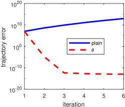
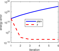
Figure 4: Maximum error of standard (solid) and $\theta$-parareal (dashed) on harmonic oscillator. The stiffness is $\omega=1$ and final time is $T=10^{3}$. Fine and coarse integrator are Velocity Verlet with step sizes $H=0.5,\;h=10^{-2}$.

Example 3.2.

Inhomogeneous linear system with variable-coefficients and singular pulses-like forcing. A low dimensional example. Consider the following forced linear system with varying coefficients,

$$\left[\begin{array}[]{c}x^{\prime}\\ y^{\prime}\end{array}\right]=A(t)\left[\begin{array}[]{c}x\\ y\end{array}\right]+b(t),$$

where $A(t)$ is a time dependent matrix of purely imaginary eigenvalues, and $b(t)$ is an external force. Figure 5, depicts results using the midpoint rule as a coarse integrator and fourth order Runge-Kutta (RK4) as a fine one. Initial conditions are $x_{0}=1,\;y_{0}=0$. The coefficient matrix is $A(t)=\left[\begin{array}[]{cc}0&1\\ -(\cos(t)^{2}+1)&0\end{array}\right]$ and the forcing term is $b(t)=\sum_{i=1}^{40}e^{-50(t-t_{i})^{2}}$ where $t_{i}$ are chosen randomly in $[0,T]$. Similar to the example above, the optimal $\theta$ is given by $\theta=\tilde{F}_{H}\tilde{C}_{H}^{-1}$. However, in this example it is time-dependent. Disregarding the forcing term,

$$\tilde{C}_{H}=\boldsymbol{1}+H\left(A(t)+\dfrac{1}{2}HA(t+\dfrac{1}{2}H)\right)$$

$$\tilde{F}_{H}=\left[\boldsymbol{1}+hA(t)+\dfrac{h^{2}}{2}A\left(t+\dfrac{h}{2}\right)A(t)+\dfrac{h^{3}}{6}A^{2}\left(t+\dfrac{h}{2}\right)A(t)+\dfrac{h^{4}}{24}A(t+h)A^{2}\left(t+\dfrac{h}{2}\right)A(t)\right]^{H/h}.$$

Thus, $\theta$ needs to be computed at every coarse time step. However, it is the same for all iterations.

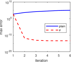
Figure 5: Error of standard (solid) and $\theta$-parareal (dashed) methods for the variable coefficient system with time varying frequencies and forcing, example 3.2. The coarse integrator is midpoint with stepsize $H=0.5$ and fine integrator is RK4 with stepsize $h=10^{-2}$. Final time $T=100$.

Example 3.3.

“De-homogenization”. In this example, we show how parareal can be used to “fill-in” the details in multiscale numerically homogenized solutions. Again, the motivation of this high-dimensional example is to demonstrate how the parareal scheme can be stabilized using a simple multiplication by a small real number $\theta$. The main point out of this example is not about an optimal solution of the PDE, but rather the feasibility of using the parareal framework for multiscale computation.

We consider the following heat equation with highly oscillatory coefficient,

$$u_{t}^{\epsilon}=\frac{\partial}{\partial x}\left(a(x,\frac{x}{\epsilon})u_{x}^{\epsilon}\right),\,\,\,0\leq x\leq 1,t>0,$$ (21)

with

$$a(x,y)=a_{0}+\sin(2\pi y)(1-e^{-100(x-0.133104)^{2}}),\,\,\,a_{0}=1.1\,\text{or}\,1.01.$$

Initial condition are $u^{\epsilon}(x,0)=x(1-x)$ and $u(0)=u(1)=0.$

The fine integrator $F_{H}$ evolves the discretized system derived from centered differencing for the right hand side of the differential equation using the classical 3-point stencil on a uniform mesh, $\{x_{j}=j\Delta x:j=1,2,\cdots,M-1\}$, with $\Delta x=\epsilon/20,\epsilon=0.04$. In parallel, each fine integration runs 50 Crank-Nicholson (CN) steps with step size $h=H/50$, with $H=2\Delta x$. The coarse integrator solves the homogenized equation

$$\bar{u}_{t}-\bar{A}\ \bar{u}_{xx}=0,\ \ \bar{A}=\begin{cases}\sqrt{0.21},&a_{0}=1.1,\\ 0.141774,&a_{0}=1.01,\end{cases}$$ (22)

on the same spatial grid, with the same initial and boundary conditions as above. Time steps are either Implicit Euler (IE) or CN, running $100$ coarse steps using $H=2\Delta x$.

Denoting the discrete solution as $u_{n}^{(k)}=(u_{1,n}^{(k)},u_{2,n}^{(k)},\cdots,u_{M-1,n}^{(k)}),$ where $u_{j,n}^{(k)}$ is the computed solution at grid node $x_{j}$ and time $nH$ at the $k$-th parareal iteration, the relative errors are given by

$$e_{n}^{(k)}:=\frac{||u_{n}^{(k)}-u_{n}^{\epsilon}||_{h}}{||u_{n}^{\epsilon}||_{h}},$$

where $u_{n}^{\epsilon}$ is the reference solution at $t=nH$, computed using Crank-Nicholson with step size $h$. The norm $||\cdot||_{h}$ is the usual 2-norm for grid functions, e.g. $||u_{n}^{(k)}||_{h}:=\left(\sum_{j=1}^{M-1}|u_{j,n}^{(k)}|^{2}\Delta x\right)^{1/2}$. We report the errors at $n=75,$ which is at 3/4 of the total simulated time steps. The purpose is simply to avoid being too close to the largest parareal iterations that we simulate.

Standard parareal ($\theta=1$) yields unstable iterations with both IE and CN, unless there is dissipation. Figure 6 depicts a comparison, with dissipation term, between different values of $\theta$ applied to the IE or CN schemes as coarse time integrators. CN scheme require smaller values of $\theta$ (i.e., the stability region is narrower). On the Fourier domain, we see that the amplification factor for IE is

$$\hat{Q}_{IE}(\omega)=\frac{1}{1+4\sigma\sin^{2}\xi/2},$$

and that of CN is

$$\hat{Q}_{CN}(\omega)=\frac{1-2\sigma\sin^{2}\xi/2}{1+2\sigma\sin^{2}\xi/2},$$

where $\sigma=\bar{A}\Delta t/\Delta x^{2}$ and $\xi=\omega\Delta x$. We see first that the parareal iterations with IE are more stable because $|\hat{Q}_{IE}|$ is smaller than $|\hat{Q}_{CN}|$ in general. Furthermore, for large $\sigma,$ $\hat{Q}_{CN}$ is close to $-1$ for $\xi\neq 0$. In our simulations, we used $\sigma=2\Delta x^{-1}$ (i.e. $\Delta t\sim\Delta x$), thus the coupling is highly unstable because $|C_{H}|\approx 1$. Figure 6 shows that a smaller value of $\theta$ is needed to stabilize the parareal iterations with CN. The price of using a smaller $\theta$ is that $|F_{H}-\theta C_{H}|$ is bigger and the overall amplification factor is not as small as that using IE.

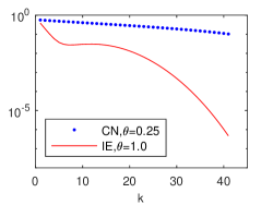
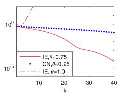
Figure 6: Stability of the multiscale couplings, considered in Example 3.3. The two subplots show the relative errors computed by different values of $\theta$ applied to the IE (Implicit Euler) and CN (Crank-Nicolson) schemes as coarse time integrators. The left subplot shows the relative errors for the case $a_{0}=1.1$ and the right subplot shows the errors for the case $a_{0}=1.01.$ The latter case is less diffusive and corresponding requires more stabilization.

Example 3.4.

Linear wave equation

$$u_{tt}=c^{2}(x)\Delta u,\,\,\,0\leq x<1,t\geq 0$$

with periodic boundary condition in $x$ and the initial conditions

$$u(x,0)=u_{0}(x):=0.1\exp(-50(x-0.5)^{2})$$

and $u_{t}(x,0)=0.$ The coarse solver will solve this problem using the wave speeds $c(x)=\bar{c}(x)\equiv 1$, and the fine solver will use the wave speed

$$c^{2}(x)=1-0.2e^{-2000(x-0.133104)^{2}}-0.1e^{-2000(x-0.733104)^{2}}.$$ (23)

Both shall use the following notations to denote the numerical approximation to the solution $u(x,t)$ and $u_{t}(x,t$):

$$\mathbf{u}_{n,j}=\left(\begin{array}[]{c}u_{n,j}\\ p_{n,j}\end{array}\right)\approx\left(\begin{array}[]{c}u(j\Delta x,n\Delta t)\\ u_{t}(j\Delta x,n\Delta t)\end{array}\right),$$

where $\Delta x$ and $\Delta t$ are respectively the grid spacings in $x$ and in $t$ used in the finite difference scheme

$$p_{n+1,j} =p_{n,j}+\Delta t\,c^{2}(j\Delta x)D_{+}^{x}D_{-}^{x}u_{n,j}-\alpha\Delta t\Delta x^{3}D_{-}^{t}(D_{+}^{x}D_{-}^{x})^{2}u_{n,j},$$ (24)

$$u_{n+1,j} =u_{n,j}+\Delta t\,p_{n+1,j},$$ (25)

with initial conditions $u_{0,j}=u_{0}(j\Delta x)$ and $p_{0,j}=0,$ $j=0,1,\cdots,\Delta x^{-1}-1$ and the boundary condition $u_{n,M}=u_{n,0},$ $n=0,1,2,\cdots,N.$ We will use $\alpha<1/15.$ The last term in (24) is a discretization of the damping term $\alpha\Delta x^{3}u_{txxxx}$ which damps out very high frequency Fourier components of solutions. The stability condition for this scheme requires that $\Delta t\leq\Delta x/2.$ We shall use the same scheme for both the coarse and the fine solver. The only difference is that the coarse solver will solve on a grid with spacing $\Delta x=H,$ $\Delta t=H/2$, and the fine on a grid with $\Delta x=H/40,$ and $\Delta t=H/80.$

We present numerical results computed by the following iterations:

$$\mathbf{u}_{n+1}^{(k+1)}=\theta_{n}^{(k)}C_{H}\mathbf{u}_{n+1}^{(k+1)}+\mathcal{P}F_{H}\mathcal{R}\mathbf{u}_{n}^{(k)}-\theta_{n}^{(k)}C_{H}\mathbf{u}_{n}^{(k)},\,\,\,0<\theta_{n}^{(k)}\leq 1.$$ (26)

Here $\mathcal{R}$ is the reconstruction operator that takes a grid function defined on $H\mathbb{Z}\cap[0,1)$ to a grid function defined on the finer grid $h\mathbb{Z}\cap[0,1)$; $\mathcal{P}$ is the projection operator that maps the grid function defined on $h\mathbb{Z}\cap[0,1)$ to a grid function on the coarser grid $H\mathbb{Z}\cap[0,1)$. In the following simulations, $\mathcal{R}$ is defined by the cubic interpolation that assuming the grid function to be periodic on $[0,1),$ while $\mathcal{P}$ is simply taken to be the pointwise restriction assuming that $H$ is divisible by $h$.

In Figures 7 and 8, we present a result computed using

$$\theta_{n}^{(k)}=\begin{cases}1,&n\leq 750\,\,\,\text{and}\,\,\,k>3,\\ 1-\frac{3}{4}(nH)\,10^{-3},&\text{otherwise.}\end{cases}$$

The simulation involves $800$ coarse steps. We found that both the stabilization term (the last term in (24)) as well as $\theta_{n}^{(k)}$ being smaller than 1 for large $n$ play important role in the stability of the parareal iterations. Standard parareal scheme typically become very unstable in the setup considered in this example. We also observe that even though the initial errors is improved by over 90% after only few iterations, improvement by further iterations is rather small. More elaborate stabilization is required if one wishes to speed up the convergence rate.

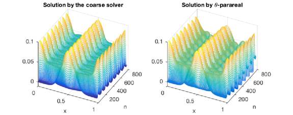
Figure 7: Example 3.4 (wave equation). Left: Solution computed by the coarse solver, without parareal coupling to the fine solver. Right: The $\theta$-parareal solution computed at $k=12$.

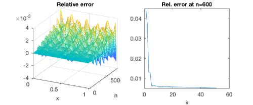
Figure 8: Example 3.4 (wave equation). Left: Pointwise errors of the $\theta$-parareal solution at $k=5$. Right: The relative error at $T_{n}=12$ (i.e. 600 coarse steps) as a function of the parareal iteration number $k$.

Example 3.5.

A spin orbit example. The following example low-dimensional Hamiltonian system as been studied in [11].

$$\left[\begin{array}[]{c}q^{\prime}\\ p^{\prime}\end{array}\right]=\left[\begin{array}[]{c}p\\ -2\epsilon\sin(q)-2\alpha\sin(2q+\phi)+14\alpha\sin(2q-\phi)\end{array}\right].$$

The initial condition is $\left[q_{0},p_{0}\right]=\left[1,0\right]$. Figure 9 presents results for standard and $\theta$-parareal where the optimal value $\theta$ is approximated at each iteration and time step using the interpolation method described in Algorithm 1. Standard parareal is unstable after a large number of steps.

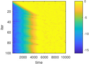
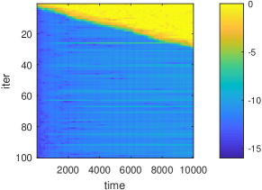
Figure 9: Log (base 10) errors of standard parareal (left) and lower dimensional interpolation based $\theta$-parareal (right) on spin orbit problem, example 3.5. The parameter is $T=10^{4},\epsilon=0.01,\alpha=10^{-4},\phi=0.2$. Velocity Verlet is used for both fine and coarse integrators with $h=10^{-2}$ and $H=1$.

Example 3.6.

The Kepler one-body problem in 2D. Consider,

$$\left[\begin{array}[]{c}q^{\prime}\\ p^{\prime}\end{array}\right]=\left[\begin{array}[]{c}p\\ -\dfrac{q}{\|q\|^{3}}\end{array}\right],\,\,\,q(0)=1-e,\;p(0)=\sqrt{\dfrac{1+e}{1-e}},$$

where $q(t)$, $p(t)\in\mathbb{R}^{2}$ and $0\leq e<1$ is the eccentricity. Larger eccentricity corresponds to stiffer problem.

In Figure 10 we present a comparison of the results computed by the standard parareal and by the interpolative $\theta$-parareal as described in Algorithm 1. Both fine and coarse solvers apply Velocity Verlet with step sizes $h=10^{-4}$ and $H=0.02$. We see that on intermediate time intervals (up to around $T=100$), the interpolative approach significantly improves both the accuracy and stability of parareal. At longer times, accuracy deteriorates for both methods, although slower with $\theta$-parareal. Sequentializing sets of parareal simulations to integrate shorter time intervals at a time greatly improves the overall accuracy of long time scales for this types of nonlinear Hamiltonian dynamics.

Figure 11 shows the local errors, $|F_{H}u_{n}^{(k+1)}-\theta_{n}^{(k)}C_{H}(u_{n}^{(k+1)})|$ with $N=1000/H=50000$ at different iterations.

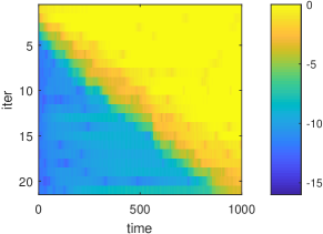
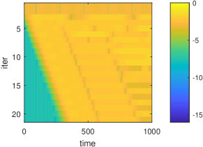
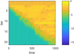
Figure 10: Log (base 10) errors of the plain parareal (left) and interpolative $\theta$-parareal (right) in trajectory (top) and energy (bottom) for Kepler system of 1 planet in 2D, example 3.6. The errors is presented in $\log_{10}$. Eccentricity is $e=0.5$. Fine and coarse integrator are Velocity Verlet with steps $h=10^{-4}$ and $H=0.02$. The largest trajectory error is about the diameter of the orbit.

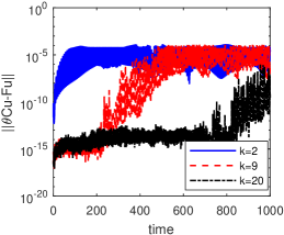
Figure 11: Example 3.6: Local errors of the improved coarse integrator $\theta_{n}^{(k)}C_{H}$.

Example 3.7.

The two-body Kepler problem in 3 dimensions. The two planets are described by $\mathbb{R}^{3}$, $j=1,2,$ leading to a nonlinear system in $\mathbb{R}^{12}$.

$$\left[\begin{array}[]{c}q_{1}^{\prime}\\ q_{2}^{\prime}\\ p_{1}^{\prime}\\ p_{2}^{\prime}\end{array}\right]=\left[\begin{array}[]{c}p_{1}\\ p_{2}\\ -\dfrac{q_{1}}{\|q_{1}\|^{3}}-10^{-5}\dfrac{q_{1}-q_{2}}{\|q_{1}-q_{2}\|^{3}}\\ -\dfrac{q_{2}}{\|q_{2}\|^{3}}+10^{-5}\dfrac{q_{1}-q_{2}}{\|q_{1}-q_{2}\|^{3}}\end{array}\right],$$

with the initial conditions is

$$q_{1}=\left[\begin{array}[]{c}1-e_{1}\\ 0\\ 0\end{array}\right],\;q_{2}=\left[\begin{array}[]{c}\cos(\pi/4)(1-e_{2})\\ 0\\ \sin(\pi/4)(1-e_{2})\end{array}\right],\;p_{1}=\left[\begin{array}[]{c}0\\ \sqrt{\dfrac{1+e_{1}}{1-e_{1}}}\\ 0\end{array}\right],\;p_{2}=\left[\begin{array}[]{c}0\\ \sqrt{\dfrac{1+e_{2}}{1-e_{2}}}\\ 0\end{array}\right].$$

In Figure 12, we present a comparison of the results computed by the standard parareal and by the interpolative $\theta$-parareal as described in Algorithm 1. Both the fine and coarse solvers are Velocity Verlet with step sizes $h=10^{-4}$ and $H=0.02$. Figure 13 shows the dimensions of the subspaces in which interpolations is computed and the corresponding computed errors.

In Figure 14, we further compare the results reported above to the one computed by sequentially applying the interpolative $\theta$-parareal algorithm in smaller time intervals, each of which involves $N^{\prime}=500/H=25000$ steps. We see that smaller total coarse time steps results in smaller amplification factor, which consequently results in a significantly improved accuracy.

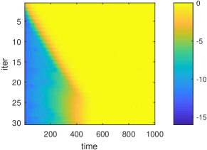
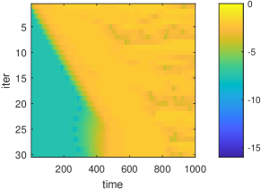
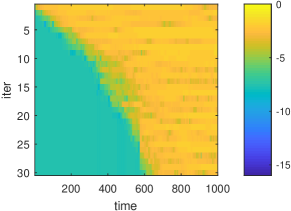
Figure 12: Log (base 10) errors of plain parareal (left column) and $\theta$-parareal lower dimension (right column). Errors in trajectory (top row) and energy (bottom row) for a Kepler system of 2 planets in 3D, example 3.8. Eccentricities are $e_{1,2}=0.4,0.5$. Fine and coarse integrator are Velocity Verlet with $h=10^{-4}$ and $H=0.02$. The interaction coefficient between the two masses is $g_{12}=10^{-5}$.

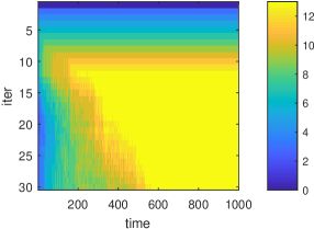
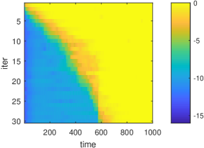
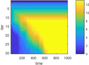
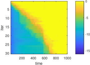
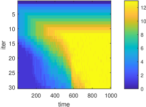
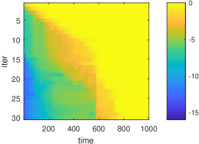
Figure 13: Number of singular values used in the subspace interpolation parareal (left column) and its corresponding errors (right column) for the two body Kepler problem in 3D, example 3.8. The tolerance parameter $tol$ in Algorithm 1 is set to $10^{-14}$ (top row), $10^{-10}$ (middle row), $10^{-6}$ (bottom row).

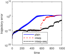
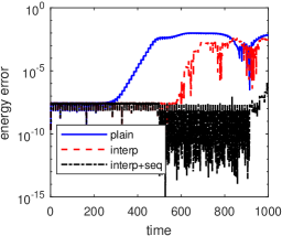
Figure 14: Error of lower dimensional interpolation $\theta$-parareal with sequential approach comparing to standard parareal on Kepler system of 2 planets in 3D, example 3.8. After $K=30$ iterations. For sequential parareal, the cut-off time is at $t=500$.

4 Summary

In this paper, we proposed a class of parallel-in-time numerical integrators, built on top of the framework of the parareal schemes. The integrators are conceived specifically with the objectives of allowing stable coupling between the chosen coarse- and fine- integrators, which may be consistent with similar but different differential equations.

The stability of parareal iterations is largely determined by the sums of amplification factor of the coarse integrator. While for dissipative problems, the amplification factor of typical schemes will be strictly less than one, purely oscillatory problems tend to preserve certain invariances and thus the amplification factor has modulus $1$. In this case, we have shown that the $\theta$-parareal method we suggest may enjoy favorable stability properties compared to the standard $\theta=1$ case.

The simplest form of the proposed scheme is a small modification to the original parareal scheme, obtained by multiplying the coarse integrator by a constant. Hamiltonian or high-dimensional systems require more complicated methods, for example, using interpolation of data points obtained in previous iterations. We analyzed the convergence of such approaches, and presented numerical simulations that enjoyed a few more digits in accuracy when compared to the results computed by the standard parareal algorithms.

References

[1]
G. Ariel, S. J. Kim, R. Tsai.
Parareal multiscale methods for highly oscillatory dynamical systems.
SIAM Journal on Scientific Computing, 38(6):A3540–A3564, 2016.
[2]
G. Bal, Q. Wu.
Symplectic parareal.
Domain decomposition methods in science and engineering XVII,
wolumen 60 serii Lect. Notes Comput. Sci. Eng., strony 401–408.
Springer, Berlin, 2008.
[3]
X. Dai, C. Le Bris, F. Legoll, Y. Maday.
Symmetric parareal algorithms for hamiltonian systems.
ESAIM: Mathematical Modelling and Numerical Analysis -
Mod?lisation Math?matique et Analyse Num?rique, 47(3):717–742, 2013.
[4]
X. Dai, Y. Maday.
Stable parareal in time method for first-and second-order hyperbolic
systems.
SIAM Journal on Scientific Computing, 35(1):A52–A78, 2013.
[5]
C. Farhat, M. Chandesris.
Time-decomposed parallel time-integrators: theory and feasibility
studies for fluid, structure, and fluid-structure applications.
International Journal for Numerical Methods in Engineering,
58(9):1397–1434, 2003.
[6]
M. Gander, E. Hairer.
Analysis for parareal algorithms applied to Hamiltonian
differential equations.
J. Comp. Appl. Math., 259:2–13, 2014.
[7]
M. J. Gander, S. G?ttel.
PARAEXP: A Parallel Integrator for Linear Initial-Value Problems.
SIAM Journal on Scientific Computing, 35(2):C123–C142, 2013.
[8]
M. J. Gander, M. Petcu.
Analysis of a Krylov Subspace Enhanced Parareal Algorithm for
Linear Problem.
ESAIM: Proc., 25:114–129, 2008.
[9]
M. J. Gander, S. Vandewalle.
Analysis of the parareal time-parallel time-integration method.
SIAM Journal on Scientific Computing, 29(2):556–578, 2007.
[10]
T. Haut, B. Wingate.
An asymptotic parallel-in-time method for highly oscillatory pdes.
SIAM Journal on Scientific Computing, 36(2):A693–A713, 2014.
[11]
H. Jiménez-Pérez, J. Laskar.
A time-parallel algorithm for almost integrable hamiltonian systems.
arXiv preprint arXiv:1106.3694, 2011.
[12]
H. B. Keller.
Numerical solution of two point boundary value problems.
SIAM, 1976.
[13]
M. Kiehl.
Parallel multiple shooting for the solution of initial value
problems.
Parallel computing, 20(3):275–295, 1994.
[14]
F. Legoll, T. Lelievre, G. Samaey.
A micro-macro parareal algorithm: application to singularly perturbed
ordinary differential equations.
SIAM J. Sci. Comput., 2013.
[15]
J.-L. Lions, Y. Maday, G. Turinici.
A "parareal" in time discretization of pde’s.
Comptes Rendus de l’Academie des Sciences, 332:661–668, 2001.
[16]
M. Minion.
A hybrid parareal spectral deferred corrections method.
Communications in Applied Mathematics and Computational
Science, 5(2):265–301, 2011.
[17]
D. Ruprecht.
Wave propagation characteristics of parareal.
arXiv preprint arXiv:1701.01359, 2017.
[18]
D. Ruprecht, R. Krause.
Explicit parallel-in-time integration of a linear acoustic-advection
system.
Computers & Fluids, 59:72–83, 2012.