A Decomposition Algorithm to Solve the Multi-Hop Peer-to-Peer Ride-Matching Problem

Abstract

In this paper, we mathematically model the multi-hop Peer-to-Peer (P2P) ride-matching problem as a binary program. We formulate this problem as a many-to-many problem in which a rider can travel by transferring between multiple drivers, and a driver can carry multiple riders. We propose a pre-processing procedure to reduce the size of the problem, and devise a decomposition algorithm to solve the original ride-matching problem to optimality by means of solving multiple smaller problems. We conduct extensive numerical experiments to demonstrate the computational efficiency of the proposed algorithm and show its practical applicability to reasonably-sized dynamic ride-matching contexts. Finally, in the interest of even lower solution times, we propose heuristic solution methods, and investigate the trade-offs between solution time and accuracy.

Neda Masoud

Assistant Professor

Department of Civil and Environmental Engineering

University of Michigan Ann Arbor, Ann Arbor, MI, USA, 48109

nmasoud@umich.edu

Corresponding author

R. Jayakrishnan

Professor

Department of Civil and Environmental Engineering

University of California Irvine, Irvine, CA, USA, 92697

rjayakri@uci.edu

1 Introduction

Recent advances in communication technology coupled with increasing environmental concerns, road congestion, and the high cost of vehicle ownership have directed more attention to the opportunity cost of empty seats traveling throughout the transportation networks every day. Peer-to-peer (P2P) ridesharing is a good way of using the existing passenger-movement capacity on the vehicles, thereby addressing the concerns about the increasing demand for transportation that are too costly to address via infrastructural expansion.

Although limited versions of P2P ridesharing systems initially emerged in the US in the 1990s, they did not receive enough support from the targeted population to continue operating. Inadequate and non-targeted marketing, insufficient flexibility and convenience, and absence of appropriate technology were some of the factors that contributed to the lack of success in implementation of the first generation of ridesharing systems.

A second generation of ridesharing systems emerged after considerable improvements in communications technology in the past few years. Making use of GPS-enabled cell phones in more recent ridesharing systems allows for accessing online information on the location of participants, making ridesharing more accessible and providing people with a sense of security. These factors combined with the high cost of travel (both financial and environmental) have played an important role in the higher levels of interest in ridesharing systems in the recent years. The high growth rate of Transportation Network Companies (TNC) such as Uber and Lyft in the USA and elsewhere in the world is an indicator of increasing levels of acceptance in the concept of outsourcing rides.

In line with the demand side, the supply side of P2P ridesharing has experienced growth as well. According to the 2009 national household travel survey (NHTS), out of an average of 4 seats available in a vehicle, only 1.7 is being actually used (Figure 1). This number is as low as 1.2 for work-based trips. In addition, number of trips per household in the US has been experiencing a decreasing trend since 1995. On the contrary, the general trend in the number of vehicles owned by households has been increasing. These statistics suggest that carpooling in households is declining, and that the number of empty seats available on traveling vehicles is increasing.

This increase on the supply side of ridesharing, coupled with the rise on the demand side, imply an optimistic future for P2P ridesharing services. This potential was recognized by the US congress in June 2012. Section 1501 of the Moving Ahead for Progress in the 21st Century (MAP-21) transportation act expanded the definition of “carpooling” to include “real-time ridesharing” as well, making ridesharing eligible for the federal funds that were previously available only for carpooling projects.

In this paper, we define P2P dynamic ridesharing to include all one-time rideshares with any type of arrangement, whether it is on-the-fly or pre-arranged, between peer drivers and riders. Dynamic ridesharing differs from more traditional carpooling services in that in carpooling shared trips are scheduled for an extended period of time, and are not one time occurrences. Furthermore, the nature of carpooling programs does not ask for real-time ride-matching.

Drivers in a ridesharing system drive to perform activities of their own, and not for the mere purpose of transporting riders. Each driver can have multiple riders on board at any point in time. In addition, to increase the number of served rider requests, the system provides multi-hop itineraries for riders, where riders may transfer between vehicles.

We define a set of stations in the network where riders and drivers can start and end their trips, and riders can transfer between vehicles. The system finds matches for riders by optimally routing drivers in the network. In order to guarantee a high quality of service, both riders and drivers provide a time window to specify the start and end of their trips, and a maximum ride time. Furthermore, riders can specify the maximum number of transfers they are willing to make, and drivers can put a limit on the number of riders they want to have on board at each moment in time. The term “real-time” emphasizes the capability of the system to make ride-matches in a short period of time, for implementation with frequent re-optimizations using newer data over time.

A P2P ride-matching algorithm is central to successful implementation of a ridesharing system. Ride-matching refers to the problem of matching riders (passengers) and drivers in a ridesharing system. A successfully matched rider receives from the system an itinerary of his/her trip that includes information on the scheduled route, and the drivers with whom the travel is planned. Drivers receive itineraries that include the schedules to pick up and drop off riders.

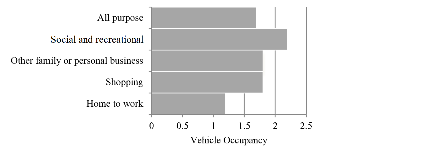
Figure 1: Average vehicle occupancy in the US in 2009 for different trip purposes (U.S. Department of Transportation, 2009)

2 Literature Review

The Multi-hop P2P ride-matching problem can be formulated as a special case of the general pick-up and delivery problem (GPDP). GPDP consists of devising a set of routes to satisfy transportation requests with given loads, and origin/destination locations. Vehicles that operate these routes each have a certain origin, destination, and capacity (Savelsbergh and Sol (1995)).

The dial-a-ride problem (DARP) is a special case of the GPDP, where all vehicles share the same origin and destination depot, and the loads to be transported are people. Although DARP is usually used in systems that aim at transporting elderly or handicapped people, this problem is very close to the ride-matching problem in ridesharing systems.

In its basic form, DARP considers a depot where a fleet of homogeneous vehicles start their trips in the morning, and to which they return at the end of their shifts. Each passenger is assumed to make the entire trip in the same vehicle, i.e., the possibility of transfers between vehicles is not considered. Variants of DARP that are more application-friendly consider time windows for the pick-up and delivery of passengers (Jaw et al., 1986; Psaraftis, 1983). Cordeau and Laporte (2007a, b) provide an overview of the literature on DARP.

In reality, the problem of transporting passengers is often more complex than the basic form of DARP. Some agencies have their fleet located at stations throughout their operating area. This has motivated the development of the multi-depot formulation for DARP (MD-DARP) (Cordeau and Laporte 2007a). Recently, Carnes et al. (2013) and Braekers et al. (2014) have added heterogeneity into the mix, and studied the multi-depot heterogeneous DARP (MD-H-DARP). These studies include heterogeneity among vehicles (multiple depots, capacity, level of service, and operating costs) as well as passengers (level of care, accompanying individuals, required resources, and total number of passengers).

An additional degree of flexibility that has recently been added to the original DARP is the possibility for passengers to transfer between multiple vehicles/modes of transportation, leading to the emergence of the DARP with transfers (DARPT). Masson et al. (2014a), Stein (1978), and Liaw et al. (1996) are the only papers that have studied this variant of the problem, to the best of our knowledge. Masson et al. (2014a) limit the number of potential transfers to one. Stein (1978) does not put a constraint on the capacity of vehicles, and works with demand at an aggregate level, rather than the individual passengers’ travel desires. Liaw et al. (1996) use heuristic algorithms to propose multi-modal routes to para-transit users. In their study, they try to route para-transit vehicles to carry passengers from their homes to bus stops, and from bus stops to their destinations.

The P2P ride-matching problem has attracted attention in academia only in the very recent years. Ride-matching problems share some of the characteristics of the more advanced DARPs, such as multiple depots and heterogeneous vehicles and passengers. Drivers in ridesharing systems are traveling to perform activities, and have distinct origin and destination locations (multi-depot), different vehicle capacities (heterogeneity), and rather narrow travel time windows. These factors can lead to the matching problems in ridesharing systems being spatiotemporally sparse, in general. One characteristic that differentiates the ride-matching problem from DARP is the fact that the set of vehicles in a ridesharing system is neither fixed (i.e., not a certain fleet size is available on a regular basis) nor deterministic (i.e., the system does not know in advance the time windows and origins and destinations of drivers’ trips). In addition, drivers who make their vehicles available in ridesharing systems are peers to the passengers who are looking for rides, and therefore measures of quality of service that are reserved only for passengers in DARPs should be extended to drivers as well in ridesharing systems.

Agatz et al. (2012) and Furuhata et al. (2013) classify ride-sharing systems based on different criteria, and discuss the challenges ridesharing systems face. In its simplest form, the ride-matching problem matches each driver with a single rider. This can be modeled as a maximum-weight bipartite matching problem that minimizes the total rideshare cost (Agatz et al., 2011).

There are also ride-matching problems that are more complex and try to take advantage of the full unused capacity of vehicles by allowing multiple riders in each vehicle. This form of ridesharing is similar to the carpooling problem where a large employer encourages its employees to share rides to and from work (Baldacci et al., 2004 and Wolfler Calvo et al., 2004). The taxi-sharing problem, as formulated by Hosni et al. (2014), also tries to reduce the cost of taxi services by having people share their rides. Herbawi and Weber (2012) have studied the problem of matching one driver with multiple riders in the context of ridesharing, and have proposed non-exact evolutionary multi-objective algorithms. Di Febbraro et al. (2013) formulate an optimization problem to model the many-to-one ridesharing systems (in which each rider is paired with only one driver, though each driver can carry multiple riders), and use optimization engines to solve it. Stiglic et al. (2015) manage to increase the number of served riders by having riders walk to meeting points, where multiple riders can be picked up by a driver. The number of stops for each driver, however, is limited to a maximum of two.

Herbawi and Weber (2011a, b) model another variant of the ride-matching problem in which a single rider can travel by transferring between multiple drivers. They propose a genetic algorithm to solve this one-to-many matching problem. Masson et al. (2014b) study a similar problem in a multi-modal environment, where goods are carried using a combination of excess bus capacities and city freighters. They propose an adaptive large neighborhood heuristic algorithm to solve the problem. Coltin and Veloso (2014) show the fuel efficiency that including transfers in the riders’ itineraries can offer, using three heuristic algorithms.

Many-to-many matching problems allow drivers to have multiple passengers on board at each point in time, and riders to transfer between drivers (Agatz et al., 2010). Cortés et al. (2010) were the first to formally formulate a many-to-many pick-up and delivery problem. They introduced an exact branch-and-cut solution method. The largest example they solved, however, consisted of 6 requests, two vehicles, and one transfer point. To the best of our knowledge, there are only two studies that model many-to-many ridesharing systems. Agatz et al. (2010) is one of the first to take an optimization approach toward modeling many-to-many ridesharing systems. In their study, the authors discuss modeling multi-modal ridesharing systems that allow for transfers between different modes of transport. However, they do not discuss a solution methodology. Ghoseiri (2013) formulates a mixed integer problem (MIP) to model the many-to-many ridesharing system. Their proposed solution heuristic limits the number of transfers to a maximum of two.

In addition to multi-hop ridesharing, a solution methodology that can handle unlimited number of transfers can be used to optimize multi-modal transportation networks, where, for example, ridesharing is combined with public transportation. In such a scenario, each public transport line acts as a driver with a fixed route in the ridesharing system. In case of a multi-modal network, allowing for higher numbers of transfers and devising algorithms that can accomplish routing and scheduling of passengers in real-time become an integral part of the system.

In this paper, we model a multi-hop P2P ridesharing system as a binary optimization problem, and propose an efficient algorithm to solve the corresponding ride-matching problem to optimality. Our model allows drivers to carry multiple riders at the same time, and riders to transfer between vehicles, and/or different modes of transportation. This leads to higher system performance, which can, to some degree, compensate for the inherent spatiotemporal sparsity in ridesharing systems. In contrary to some ridesharing systems who either assume a given route for drivers, or allow for only limited detours from a given route, we leave the routing of the drivers to the system as a default, unless drivers specifically ask to take certain routes. In order to ensure that the higher performance of the system does not come at the cost of poor quality of service, we require both drivers and riders to have specified a maximum ride time, and for riders to have set a limit on the number of transfers. To ensure that rides can be successfully accomplished within the requested time windows specified by participants, the formulation is devised to use time-dependent travel time matrices.

The contributions of this paper to the literature are three-fold; we formulate the many-to-many ride-matching problem as a binary program in a time-expanded network, introduce a pre-processing procedure to reduce the size of the proposed optimization problem, and devise a decomposition algorithm to solve the large-scale ride-matching problem to optimality by means of iteratively solving smaller problems. The combination of the three aforementioned methodological contributions allows for the ride-matching problem to be solved in a very short period of time, enabling dynamic implementation of multi-hop ridesharing.

In the rest of the paper, we first introduce the ridesharing system to provide the context in which we need to solve the ride-matching problem. The rest of the paper focuses on formulating and solving the ride-matching problem. We start by formulating the multi-hop P2P ride-matching problem as an optimization problem. Since solving this problem directly using optimization engines is computationally prohibitive, we introduce a pre-processing procedure to limit the size of the input sets to the optimization problem, and a decomposition algorithm to solve the problem more efficiently in terms of computing time. Finally we address the scalability of the problem and real-time implementation strategies for the underlying system, and introduce heuristics to speed up reaching a high quality solution.

3 Ridesharing System

The ridesharing system defined in this paper contains a set of participants $P$. These participants are divided into a set of riders, $R$, who are looking for rides, and a set of drivers, $D$, who are willing to provide rides ($P=R\cup D$). Drivers may have different incentives to participate in the ridesharing system, including monetary compensation, using high occupancy vehicle (HOV) lanes, or reduced-cost parking, among others. Different driver incentives for ridesharing can translate into different objective functions for the corresponding ride-matching problem.

To facilitate pick-ups and drop-offs, a set of stations, $S$, are identified in the network. Stations are pre-specified locations where participants can start and end their trips, and riders can switch between drivers and/or to other modes of transport, such as transit. Strategic identification of stations is central to the performance of the system. Lessons learned from the previous P2P ridesharing systems suggest that it is better for riders to be picked up/dropped off at pre-specified locations, rather than their homes (or the exact location where their trips start/end) for two reasons (Heinrich, 2010). First, these locations could be hard to find for drivers, and therefore riders could miss their scheduled rides. In addition, drivers could have a hard time finding an appropriate location to park their vehicles. Second, some drivers and riders would understandably be reluctant to reveal their home address to others. In addition, as shown by Stiglic et al. (2015), introducing stations can increase the number of successful matches, as a result of increasing the spatial proximity between trips.

Every active participant $p$ of the rideshare system provides to the system their origin and destination stations ($OS_{p}$ and $DS_{p}$, respectively), the earliest acceptable time to depart from the origin station, $T_{p}^{ED}$, the latest acceptable time to arrive at the destination station, $T_{p}^{LA}$, and their maximum ride time, $T_{p}^{TB}$. Subsequently, the travel time window for participant $p$ can be defined as $TW_{p}=[T_{p}^{ED},T_{p}^{LA}]$. In addition, each participant is asked to provide a notification deadline by which they need to be informed of any matches made for them. Figure 2 demonstrates some of the parameters of the system.

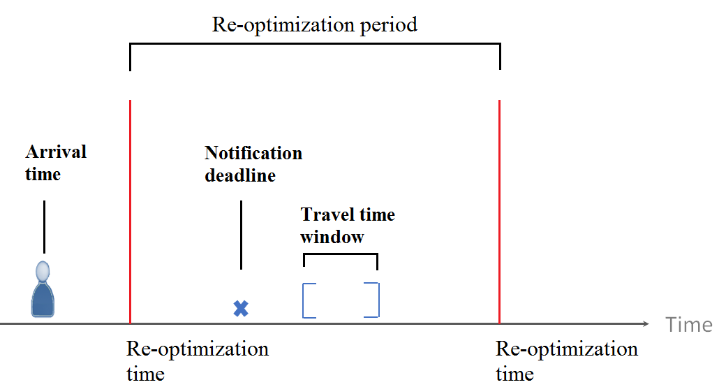
Figure 2: System parameters

Drivers should announce the capacity of their vehicles, $C_{d}$. This could simply be the physical vehicle capacity, or the maximum number of riders a driver is willing to carry in their vehicle at any point in time. Riders can specify the maximum number of transfers (change of vehicles), $V_{r}$, they are willing to make to get to their destinations.

We discretize the study time horizon into an ordered set of indexed time intervals of small duration, $\Delta t$, to allow for using time-dependent travel-time matrices. We define set $T_{p}$ to contain the indices for all time intervals within the range $TW_{p}=[T_{p}^{ED},T_{p}^{LA}]$ for participant $p$.

In a system discretized in both time and space, we define a node $i$, $n_{i}$, as a tuple $(t_{i},s_{i})$, where $t_{i}$ is the time interval one may be located at station $s_{i}$. Subsequently, a link $\ell$ is defined as $(n_{i},n_{j})=(t_{i},s_{i},t_{j},s_{j})$, where $t_{i}$ is the time interval one has to leave station $s_{i}$, in order to arrive at station $s_{j}$ during time interval $t_{j}$. We generate links between neighboring stations only, i.e., a link exists between stations $s_{i}$ and $s_{j}$ if traveling from $s_{i}$ to $s_{j}$ does not require passing through another station. Naturally, the links are determined by the travel time matrix, which could be time-dependent, and travel times used must ensure that a traveler leaving at the very end of the time interval of $t_{i}$ can arrive at least by the very end of the time interval $t_{j}$. We denote the set of links by $L$.

Figure 3 demonstrates an example of a link in a time-expanded network. If a participant leaves station 1 at time interval $1$, they arrive at station $2$ at time interval $2$. The starting and ending nodes of this trip are $n_{s}=(t_{s},s_{s})=(1,1)$, and $n_{e}=(t_{e},s_{e})=(2,2)$, respectively. The resulting link is $\ell=(t_{s},s_{s},t_{e},s_{e})=(1,1,2,2)$. In this figure we can also see link $(2,2,3,4)$. These two links together form a path that leaves station $1$ at time interval $1$, and arrives at station $4$ at time interval $3$.

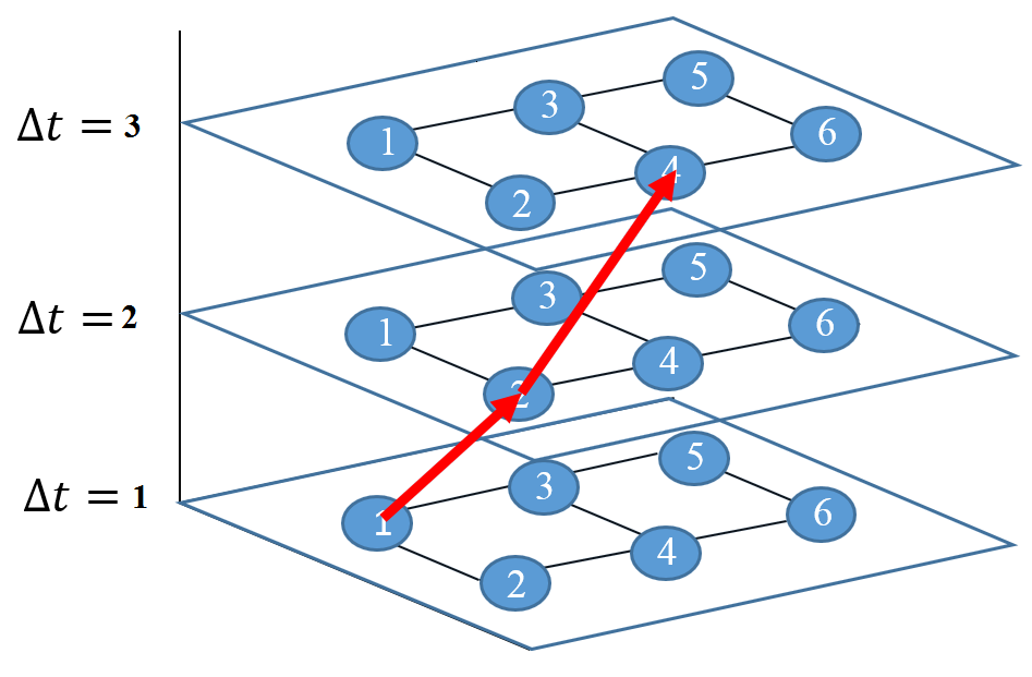
Figure 3: Example of links in a time-expanded network

The goal of the ridesharing system in this paper is to maximize the matching rate (although the proposed methodology can be used for a variety of objective functions.) For now, let us assume that drivers leave the route choice to the system. This does not preclude the case of drivers who want to follow their own fixed routes, as those routes can be specified as successive nodes and entered into the formulation as fixed parameters.

We include a dummy driver, $d^{\prime}$, in the set of drivers, and form the set $D^{\prime}=D\cup\{d^{\prime}\}$. The dummy driver has neither a real origin or destination, nor a travel time window. The motivation behind introducing the dummy driver will be explained in the following section.

The implementation strategy of a ridesharing system should be determined based on the nature of customer arrivals. Here, we adapt a general rolling time horizon framework in which the system is re-optimized periodically at pre-specified points in time called “re-optimization times”. We call the time window between two consecutive re-optimization times the “re-optimization period” (Figure 2). Re-optimizing the system allows for enhancing the reliability of the system and improving its performance by incorporating the latest information on link travel times and customer arrivals, respectively. In a rolling time horizon framework, at each re-optimization time the system solves a matching problem that includes all registered participants whose notification deadlines are after the re-optimization time. In addition, all previously matched drivers who have not finished their trips at the re-optimization time can be included in the matching problem as well, albeit if they have empty seats left, and considering their prior commitments. After solving the problem at each re-optimization time, the itineraries of matched drivers and riders whose notification deadlines lie within the first re-optimization period will be fixed and announced to them.

As previously mentioned, the rolling time horizon framework is a general framework whose parameters (i.e., the re-optimization period and re-optimization times) can be calibrated based on the distribution of customer arrivals. In an extreme case where all system participants register their trips before the onset of the planning horizon (e.g., before the start of a morning peak hour), the general rolling time horizon framework turns into a static framework. On the other side of the spectrum, if all participants arrive in real-time (i.e., their arrival times and notification deadlines are less than a few minutes apart), the rolling time horizon framework can be used to serve such a dynamic system by selecting very small re-optimization periods (e.g., 1-min periods).

4 The Multi-hop P2P Ride-Matching Problem

The role of the ride-matching problem is to devise itineraries that can take riders to their destinations by optimally routing drivers. Itineraries have to comply with the riders’ specified maximum number of transfers, the capacity of drivers’ vehicles, and the participants’ travel time windows and maximum ride times. The ride-matching problem will devise itineraries for the matched riders in the system, and all drivers, matched or not.

To mathematically model the ride-matching problem, we use four sets of decision variables, as defined in (1)-(4).

$$x_{\ell}^{d} =\begin{cases}1&\mbox{Driver $d$ travels on link $\ell$}\\ 0&\mbox{Otherwise}\end{cases}$$ (1)

$$y_{\ell}^{rd} =\begin{cases}1&\mbox{Rider $r$ travels on link $\ell$ with driver $d$}\\ 0&\mbox{Otherwise}\end{cases}$$ (2)

$$z_{r} =\begin{cases}1&\mbox{Rider $r$ is matched}\\ 0&\mbox{\mbox{Otherwise}}\end{cases}$$ (3)

$$u_{r}^{d} =\begin{cases}1&\mbox{Driver $d$ contributes to the itinerary for rider $r$}\\ 0&\mbox{\mbox{Otherwise}}\end{cases}$$ (4)

Equation (5a) presents the objective function of the problem. A ride-matching problem can have various objectives, ranging from maximizing profits to minimizing the total miles/hours traveled in the network. This objective can vary depending on the nature of the agency that is managing the system (public or private), the level of acceptance of the system in the target community, and the ridesharing incentives. For a ridesharing system in its infancy, it is logical to maximize the matching rate. We use this objective for the ridesharing system in this paper.

The first term in (5a) maximizes the total number of served riders, while the second term minimizes the total number of transfers in the system, and is added only for the purposes described in Proposition 1 (in the Appendix). The weight $W_{r}$ should be set to a proper value (any value smaller than $\nicefrac{{1}}{{V_{r}}}$, where $V_{r}$ is the maximum number of transfers rider $r$ is willing to make) to ensure that serving the maximum number of riders remains the primary objective of the system.

The sets of constraints that define the ridesharing system are presented in (5b)-(5z). Constraint sets (5b)-(5g) route drivers in the network. Constraint set (5b) directs drivers in set $D$ out of their origin stations, and (5c) ensures that they end their trips at their destination stations. Note that we do not use a separate set of constraints to enforce the travel time windows for drivers. Such constraints can be satisfied automatically by limiting the set of links in constraint sets (5b) and (5c) to the ones whose time intervals are within the driver’s travel time window (in set $T_{d})$.

Constraint set (5g) is for flow conservation, enforcing that a driver entering a station in a time interval, exits the station in the same time interval. Notice that participants might not physically leave a station. Members of the link set $L$ in the form $(t,s,t+1,s)$ represent the case where a participant is physically remaining at station $s$ for one time interval, but technically leaving node $(t,s)$ for node $(t+1,s)$. In addition, constraint set (5g) enforces the multi-hop property of the ridesharing system. Riders can enter a node with a driver, and exit it with a different driver, suggesting a transfer between the two drivers (or modes of transportation). Constraint set (5h) limits the total travel time by drivers based on their maximum ride times.

Max $$\;\;\sum_{\medspace\medspace\medspace r\in R}z_{r}-\sum_{r\in R}W_{r}\sum_{d\in D}u_{r}^{d}$$ (5a)

Subject to: $$\sum_{{}^{{}_{s_{i}=OS_{d}(t_{i},t_{j})\in T{}_{d}}^{\quad\>\;\;\quad\ell\in L:}}}\!\!\!\!\!\!\!\!\!\!x_{\ell}^{d}\>\>\>\>-\quad\!\!\!\!\!\!\!\!\!\sum_{{}^{{}_{s_{j}=OS_{d};t_{i},t_{j}\in T{}_{d}}^{\quad\>\;\;\quad\ell\in L:}}}\!\!\!\!\!\!\!\!\!\!x_{\ell}^{d}=1 \forall d\in D$$ (5b)

$$\sum_{{}^{{}_{s_{j}=DS_{d};t_{i},t_{j}\in T{}_{d}}^{\quad\>\;\;\quad\ell\in L:}}}\!\!\!\!\!\!\!\!\!\!x_{\ell}^{d}\>\>\>\>-\quad\!\!\!\!\!\!\!\!\!\sum_{{}^{{}_{s_{i}=DS_{d};t_{i},t_{j}\in T{}_{d}}^{\quad\>\;\;\quad\ell\in L:}}}\!\!\!\!\!\!\!\!\!\!x_{\ell}^{d}=1 \forall d\in D$$ (5c)

$$\;\;\sum_{{}_{\ell=(t_{i},s_{i},t,s)\in L}^{\qquad t_{i},s_{i}}}\!\!\!\!\!x_{\ell}^{d}\>\>\>=\!\!\!\!\!\!\sum_{{}_{\ell=(t,s,t_{j},s_{j})\in L}^{\qquad t_{j},s_{j}}}\!\!\!\!\!x_{\ell}^{d} \!\!\!\begin{array}[]{l}\forall d\in D\\ \forall t\in T_{d}\\ \forall s\in S\backslash\{OS_{d}\cup DS_{d}\}\end{array}$$ (5g)

$$\;\;\sum_{{}^{\ell\in L}}(t_{j}-t_{i})x_{\ell}^{d}\leq\frac{T_{d}^{TB}}{\Delta t} \forall d\in D$$ (5h)

$$\>\>\sum_{{}^{d\in D^{\prime}}}\!\!\!\sum_{{}^{{}_{s_{i}=OS_{r};t_{i},t_{j}\in T{}_{r}}^{\quad\>\;\;\quad\ell\in L:}}}\!\!\!\!\!\!y_{\ell}^{rd}-\sum_{{}^{\quad d\in D^{\prime}}}\!\!\!\sum_{{}^{{}_{s_{j}=OS_{r};t_{i},t_{j}\in T{}_{r}}^{\quad\>\;\;\quad\ell\in L:}}}\!\!\!\!\!\!y_{\ell}^{rd}=z_{r} \forall r\in R$$ (5i)

$$\>\>\sum_{{}^{d\in D^{\prime}}}\!\!\!\sum_{{}^{{}_{s_{j}=DS_{r};t_{i},t_{j}\in T{}_{r}}^{\quad\>\;\;\quad\ell\in L:}}}\!\!\!\!\!\!y_{\ell}^{rd}-\sum_{{}^{d\in D^{\prime}}}\!\!\!\sum_{{}^{{}_{s_{i}=DS_{r};t_{i},t_{j}\in T{}_{r}}^{\quad\>\;\;\quad\ell\in L:}}}\!\!\!\!\!\!y_{\ell}^{rd}=z_{r} \forall r\in R$$ (5j)

$$\>\>\sum_{{}^{d\in D^{\prime}}}\!\!\!\sum_{{}^{{}_{\ell=(t_{i},s_{i},t,s)\in L}^{\qquad t_{i},s_{i}:}}}\!\!\!\!\!y_{\ell}^{rd}=\sum_{{}^{\quad d\in D^{\prime}}}\!\!\!\sum_{{}^{{}_{\ell=(t,s,t_{j},s_{j})\in L}^{\qquad t_{j},s_{j}:}}}\!\!\!\!\!y_{\ell}^{rd} \!\!\!\begin{array}[]{l}\forall r\in R\\ \forall t\in T_{r}\\ \forall s\in S\backslash\{OS_{r}\cup DS_{r}\}\end{array}$$ (5n)

$$\>\>\sum_{d\in D^{\prime}}\>\>\>\>\sum_{{}^{\ell\in L}}(t_{j}-t_{i})y_{\ell}^{rd}\leq\frac{T_{r}^{TB}}{\Delta t} \forall r\in R$$ (5o)

$$\>\>\sum_{r\in R}y_{\ell}^{rd}\leq C_{d}x_{\ell}^{d} \!\!\!\begin{array}[]{l}\forall d\in D\\ \forall\ell\in L\end{array}$$ (5r)

$$\;\;u_{r}^{d}\geq y_{\ell}^{rd} \!\!\!\begin{array}[]{l}\forall r\in R\\ \forall d\in D\\ \forall\ell\in L\end{array}$$ (5v)

$$\;\;u_{r}^{d}\leq\sum_{\ell\in L}y_{\ell}^{rd} \!\!\!\begin{array}[]{l}\forall r\in R\\ \forall d\in D\end{array}$$ (5y)

$$\>\>\sum_{d\in D}u_{r}^{d}-1\leq V_{r} \forall r\in R$$ (5z)

Rider $r$’s itinerary is determined by variable $y_{\ell}^{rd}$. A value of $1$ for this variable indicates that the rider is traveling on link $\ell$ in driver $d$’s vehicle. By definition, this variable implies that a rider should always be accompanied by a driver. However, in reality, a rider does not need to be accompanied when he/she is traveling on a link in the form $(t,s,t+1,s)$, i.e., staying at station $s$, waiting to make a transfer. To incorporate this element into the formulation, we introduce the dummy driver $d^{\prime}$. As mentioned before, the dummy driver does not have a real origin or destination in the network. The set of links used by the dummy driver is also different from the members of the link set $L$. We define the set of links for the dummy driver as $L^{\prime}=\{(t,s,t+1,s),\forall(t,s)\in T\times S\}$. This set includes all the links that represent staying at a station for one time interval.

Constraint sets (5i)-(5n) route riders in the network, and are analogous to (5b)-(5g), except for a small variation. While the optimization problem generates itineraries for all drivers, matched or not, this is not the case for riders. Only riders who are successfully matched will receive itineraries. This difference is reflected in the formulation by replacing $1$ on the ride hand side of constraint sets (5b)-(5c) by $z_{r}$ in constraint sets (5i)-(5j). Constraint set (5o) sets a limit on the riders’ maximum ride times.

Constraint set (5r) serves two purposes. First, it ensures that riders are accompanied by drivers throughout their trips. Second, it ensures that vehicle capacities are not exceeded. Constraint sets (5v)-(5z) collectively set a limit on the total number of transfers for each rider. Constraint sets (5v) and (5y) register drivers who contribute to each rider’s itinerary (refer to Proposition 2 in the Appendix). Constraint set (5z) restricts the number of transfers by each rider (refer to Proposition 1 in the Appendix). Finally, all decision variables of the problem defined in (1)-(4) are binary variables.

Although the formulation in model (5) is defined for a ridesharing system in its infancy, it is easy to include additional terms in the objective function or introduce additional decision variables and constraint sets to cover different objectives ridesharing systems may have throughout their lifetime. For instance, we can minimize the total travel time by riders and drivers by adding terms $\sum_{d\in D}\sum_{r\in R}\sum_{\ell\in L}(t_{j}-t_{i})y_{\ell}^{rd}$ and $\sum_{d\in D}\sum_{\ell\in L_{d}}(t_{j}-t_{i})x_{\ell}^{d}$ to the objective function, respectively. It is possible to minimize/maximize the number of matched drivers by introducing the decision variable $z_{d}^{\prime}$ that takes the value of 1 is driver $d$ is matched, and $0$ otherwise. In this case, the unit values on the right hand sides of constraint sets (5b) and (5c) should be replaced with $z_{d}^{\prime},$ and the term $W^{\prime}\sum_{d\in D}z_{d}^{\prime}$ should be added to the objective function.

In the formulation presented in model (5), we do not consider an exclusive service time for participants. This can be a realistic assumption, since we are concerned with people and not goods. However, if service times are required due to practical considerations, they can be easily integrated by making small changes in the definition of the link sets and constraint sets (5g) and (5n). Originally, we defined a link between two stations $s_{i}$ and $s_{j}$ if the two stations were neighboring stations in the network. To account for service times, we have to redefine the link sets to include links between any two stations. If a rider travels from their origin station to station $k$, and then from station $k$ to their destination station, this implies a transfer at station $k$. To include service times, equations (5g) and (5n) should be replaced with constraint sets (6) and (7), respectively, where $t_{s}$ is the service time (in number of time intervals).

$$\!\!\!\!\!\!\!\!\sum_{{}_{\ell=(t_{i},s_{i},t,s)\in L}^{\qquad t_{i},s_{i}}}\!\!\!\!\!\!x_{\ell}^{d}\qquad=\!\!\!\!\!\!\!\sum_{{}_{\ell=(t+t_{s},s,t_{j},s_{j})\in L}^{\qquad t_{j},s_{j}}}\!\!\!\!\!\!x_{l}^{d}\quad\forall d\in D,\forall t\in T_{d},\forall s\in S\backslash\{OS_{d}\cup DS_{d}\}$$ (6)

$$\sum_{{}^{d\in D^{\prime}}}\!\!\!\!\!\!\sum_{{}_{\ell=(t_{i},s_{i},t,s)\in L}^{\qquad\!\!\!\!t_{i},s_{i}:}}\!\!\!\!\!\!y_{\ell}^{rd}=\sum_{{}^{d\in D^{\prime}}}\!\!\!\!\!\!\!\!\sum_{{}_{\ell=(t+t_{s},s,t_{j},s_{j})\in L}^{\qquad t_{j},s_{j}:}}\!\!\!\!\!\!\!\!y_{\ell}^{rd}\quad\forall r\in R,\forall t\in T_{r},\forall s\in S\backslash\{OS_{r}\cup DS_{r}\}$$ (7)

Solving the optimization problem in model (5) is computationally prohibitive, even for small instances of the problem. Therefore, in its original form, the ride-matching problem in model (5) is not appropriate for time-sensitive applications. In the next section, we introduce a pre-processing procedure that reduces the size of the input sets to the optimization problem. Subsequently, we propose a decomposition algorithm that attempts to solve the original ride-matching problem by means of iteratively solving multiple smaller problems called “sub-problems”.

5 Pre-processing Procedure

The goal of the pre-processing procedure is to limit the number of accessible links for each participant, and identify and eliminate drivers who cannot be part of a rider’s itinerary due to lack of spatiotemporal compatibility between their trips. At the onset, it should be noted that this procedure does not limit the search space of the optimization problem, but only narrows it by cutting down practically infeasible ranges, and therefore it does not affect the optimality of the solution.

As explained before, we present a link, $\ell$, as a 4-tuple $(t_{i},s_{i},t_{j},s_{j})$. Participants can potentially reach any station in the network in any time interval within their travel time window, making the size of the set of links, $L$, as large as $O(|T||S|)$, where $|T|$ is the number of time intervals in the study time horizon, and $|S|$ is the number of stations in the network.

The premise of the pre-processing procedure is that the spatiotemporal constraints enforced by maximum ride times and travel time windows of participants limit their access to members of the link set $L$. We use this information to construct the set of links accessible to riders and drivers, denoted by $L_{r}$ and $L_{d}$, respectively.

The origin and destination stations, maximum ride times, and travel time windows of participants can be used to define a region in the network in the form of an ellipse, inside which participants have a higher degree of space proximity, i.e., the percentage of accessible stations within this region is at least as high as the same percentage within the entire network. We call the region inside and on the circumference of the ellipse associated with participant $p$ the reduced graph of the participant, denoted by $G_{p}$ (reduced graph of rider $r$/driver $d$ is denoted as $G_{r}/G_{d}$). The focal points of the ellipse are the participant’s origin and destination stations. The length of the major axes between the focal points is the straight distance between the origin and destination stations, and the transverse diameter of the ellipse is an upper-bound on the distance that can be traveled by the participant in $\frac{T_{p}^{TB}}{\Delta t}$ number of time intervals, within the participant’s travel time window.

We know that for each point on the circumference of an ellipse, sum of the distances from the two focal points is always constant, and equal to the transverse diameter of the ellipse. By setting the length of the transverse diameter to the maximum distance a participant can travel given their travel time window, we ensure that none of the stations outside of the participant’s reduced graph are accessible to them.

After the reduced graphs are generated, we use the link reduction algorithm presented in Algorithm 1 to construct sets $L_{r}$ and $L_{d}$. The algorithm finds the set of links for participant $p$ in two steps: a forward movement followed by a backward movement. Both forward and backward movements are iterative procedures. We start the algorithm by defining sets $T_{s}$ and $L(s)$ for all stations $s\in G_{p}$ and initializing them to be empty, where $T_{s}$ is the set of time intervals during which station $s$ can be reached, and $L(s)$ is the set of links terminating at station $s$ (line 2).

Algorithm 1 Link reduction algorithm

Generate a link set $L_{p}$ for participant $p$

$01\quad$Initialize

$02\quad$ $T_{s}=\emptyset,\;L(s)=\emptyset,\;\forall s\in G_{p}$

$03\quad$ Step1. Forward movement

$04\quad$ $S_{act}=\{OS_{p}\}$

$05\quad$ $\bar{S}_{act}=\emptyset$

$06\quad$ $T_{OS_{p}}=\{\frac{T^{ED}_{p}}{\Delta t},\frac{T^{ED}_{p}}{\Delta t}+1,\frac{T^{ED}_{p}}{\Delta t}+2,...,\frac{T_{p}^{LA}-T_{static}(OS_{p},DS_{p})}{\Delta t}\}$

$07\quad$ While $S_{act}\not=\emptyset$

$08\quad$ $\qquad s_{1}\leftarrow S_{act}(1)$

$09\quad$      For $s\in\{S\backslash OS_{p}\}$

$10\quad$            Set $T_{s_{1}}=T_{s_{1}}\cup\{t_{1}\}$ such that $\exists\>\ell=(t,s,t_{1},s_{1})\in L(s),\forall(t,t_{1})\in T_{p}^{2}$

$11\quad$      End For

$12\quad$ $\qquad S_{act}=S_{act}\backslash\{s_{1}\}$

$13\quad$ $\qquad\bar{S}_{act}=\bar{S}_{act}\cup\{s_{1}\}$

$14\quad$      For $s_{2}\in S:(s_{1},s_{2})\in G_{p}$

$15\quad$           If $s_{2}\cap\bar{S}_{act}=\emptyset$

$16\quad$ $\qquad\qquad\qquad S_{act}=S_{act}\cup\{s_{2}\}$

$17\quad$                For $t\in T_{s_{1}}$

$18\quad$                $\qquad L(s_{2})=L(s_{2})\cup\{(t,s_{1},t+T_{dynamic}(t,s_{1},s_{2})^{\dagger}$$,s_{2})\}$

$19\quad$                End For

$20\quad$           Else

$21\quad$                For $t\in T_{s_{1}}$

$22\quad$                     If $T_{s_{2}}\cap\big{\{}t+T_{dynamic}(t,s_{1},s_{2})\big{\}}\neq\emptyset$

$23\quad$ $\qquad\qquad\qquad\qquad\qquad L(s_{2})=L(s_{2})\cup\{(t,s_{1},t+T_{dynamic^{\dagger}}(t,s_{1},s_{2}),s_{2})\}$

$24\quad$                     End If

$25\quad$                End For

$26\quad$           End If

$27\quad$      End For

$28\quad$ End While

$29\quad$ Step 2. Backward movement

$30\quad$ $L_{del}=\{(t_{1},s_{1},t_{2},s_{2})\in L_{p}:(s_{2}=DS_{p})\wedge(t_{2}>\frac{T_{p}^{LA}}{\Delta t})\}$

$31\quad$ While $L_{del}\not=\emptyset$

$32\quad$ $\qquad\ell(t_{1},s_{1},t_{2},s_{2})\leftarrow L_{del}(1)$

$33\quad$ $\qquad L_{del}=L_{del}\backslash\{\ell\}$

$34\quad$ $\qquad L_{p}(s_{2})=L_{p}(s_{2})\backslash\{\ell\}$

$35\quad$      For $s_{1}\in G_{p}$

$36\quad$           For $(t,s):(t,s,t_{1},s_{1})\in L_{p}(s_{1})$

$37\quad$ $\qquad\qquad\quad L_{del}=L_{del}\cup\{(t,s,t_{1},s_{1})\}$

$38\quad$           End For

$39\quad$      End For

$40\quad$ End While

$41\quad$ Generating Link set $L_{p}$

$42\quad$ $L_{p}=\bigcup_{s\in G_{p}}L(s)$

$43\quad$ ${}^{\dagger}T_{dynamic}(t,s_{1},s_{2}):$ travel time between stations $s_{1}$ and $s_{2}$ at time interval $t$

In each iteration the forward movement generates a set of links originating from one of the stations in the reduced graph of participant $p$. We start the forward movement by defining the set of active stations, $S_{act}$, and initializing this set with the origin station of participant $p$ (line 4). The time intervals during which this origin station can be reached can be easily computed using the equation in line 6, where $T_{static}(s_{1},s_{2})$ denotes the shortest path travel time between stations $s_{1}$ and $s_{2}$. Set $T_{OS_{p}}$ in line 6 maintains indices of time intervals during individual $p$’s travel time window. To ensure that no feasible links are eliminated, $T_{static}$ should contain underestimated link travel times, say, for example, the travel times during non-peak hours. The algorithm then selects the first member of the active stations set, denoted by $s_{1}$ (line 8), and updates the set of time intervals during which $s_{1}$ can be reached by examining all the previously generated links that terminate at $s_{1}$ (lines 9-11). Once station $s_{1}$ has been processed (i.e., the time intervals during which this station can be reached are obtained), this station will be removed from set $S_{act}$ (line 12), and added to set $\bar{S}_{act}$ (line 13), which maintains a list of previously processed stations. Note that adding station $s_{1}$ to set $\bar{S}_{act}$ does not mean that the set $T_{s_{1}}$ is finalized; we might need to revise this set later, as the participant may need to visit a station more than once if their travel time window allows (e.g., a driver may visit a station twice to pick up different passengers that start their trips at different time intervals).

Next, outgoing links from $s_{1}$ whose end stations are inside the reduced graph are identified (line 14) and their end stations are added to the set of active stations (line 16). At this point, we have information on the starting station $(s_{1})$, ending stations ($s_{2}:(s_{1},s_{2})\in G_{p})$ and the starting time intervals at $s_{1}$ $(T_{s_{1}})$. The ending time intervals for each $s_{2}$ can be easily looked up from a dynamic (i.e., time-dependent) travel time matrix, $T_{dynamic}$, completing the information required to construct the set of links originating at $s_{1}$ (lines 17-19). Note that once we identify station $s_{2}$ on the reduced graph, the process of generating $L(s_{2})$ will be slightly different depending on whether $s_{2}$ is a member of set $\bar{S}_{act}$ (lines 17-19) or not (lines 21-25), ensuring that a single link is not added to the link set multiple times. We iterate the forward movement until the set of active stations becomes empty.

Figure 4 demonstrates an example of the forward movement for a participant who is traveling from station $14$ to station $8$, with $TW_{p}=[1,40](\Delta t=1$ min$)$, maximum ride time of $40$ minutes, and shortest path travel time of $38$ minutes. Link travel times (in minutes) are shown on the graph. It is assumed that the travel time remains constant on each link. Note that this assumption is made only for simplicity, and using time-dependent travel times would be just as straightforward. The set of links for each station is computed during the forward movement, and is presented in the Figure 4. These links are not final, however, and have to be refined during the backward movement.

The backward movement simply scans through the set of links generated for each station by the forward movement and refines these sets by removing the time intervals that are identified as infeasible based on the participant’s latest arrival time. The backward movement starts by identifying links that take the participant to his/her destination station after the participant’s latest arrival time, and adds these links to set $L_{del}$, which is initially defined as an empty set (line 30). The algorithm then goes through the members of set $L_{del}$ one by one. For each member $\ell=(t_{1},s_{1},t_{2},s_{2})$, it removes $\ell$ from set $L_{p}(s_{2})$ (line 34), identifies links with end nodes $(t_{1},s_{1})$ (line 36), and adds these links to set $L_{del}$ (line 37). The backward movement ends when set $L_{del}$ becomes empty. At this point, the union of all the remaining links $L(s),\forall s\in G_{p}$ yields the set of links for participant $p$ (line 42).

In the example shown in Figure 4, since the latest arrival time is at $\Delta t=40$, links with ending time intervals $41$ and $42$ should be removed from the set of links for the destination station. Tracking back the stations from destination to origin, the time intervals for the stations that have led to the infeasible time intervals at the destination station are identified and removed (see Algorithm 1 for details). For the example in Figure 4, after completing the backward movement, the set of links, $L_{p}$, is derived and listed in the figure.

Figure 4: An example of forward and backward movements for a participant with $OS_{p}=14$, $DS_{p}=3$, $\Delta t=1$ min, $TW_{p}=[1,40]$, and $T_{p}^{TB}=40$ min

Once the set of links for participants are generated, we can use these sets to reduce the size of some other sets in the optimization problem, namely the set of riders and drivers. We can reduce the size of the rider set $R$ by filtering riders out of the problem based on their accessibility to potential drivers. For a rider to be served, they should have spatiotemporal proximity with at least one driver at both their origin and destination stations. Riders of set $R$ who do not enjoy this spatiotemporal proximity can be filtered out.

In addition, in order for a driver $d$ to be able to contribute to the itinerary of a rider $r$, the intersection of link sets of the two should not be empty, i.e., $L_{r}\bigcap L_{d}\neq\emptyset$. We denote by $M$ the set of tuples $(r,d)\in R\times D$ for whom $L_{r}\bigcap L_{d}\neq\emptyset$ and therefore could potentially be matched. For members of set $M$, we construct a set $L_{rd}=\{L_{r}\bigcap L_{d}\}$. Furthermore, we add tuples $(r,d^{\prime})$ to set $M$, and set $L_{rd^{\prime}}=L^{\prime}$ for all the unfiltered riders $r\in R$.

Note that the ellipses that form boundaries of the reduced graphs strictly prevent any feasible links from being cut off, and therefore the link set $L$ can be safely replaced by $L_{p},\forall p\in P$. Furthermore, since the potential drivers for each rider are determined based on the reduced graphs, no potential driver is excluded from the set of eligible drivers for each rider. Hence, using the refined input sets generated by the pre-processing procedure in the ride-matching problem does not affect the optimal matching of riders and drivers.

6 Decomposition Algorithm

The decomposition algorithm attempts to solve the original ride-matching problem via iteratively solving a number of smaller problems called “sub-problems” that are easier to solve. The algorithm pseudo-code is described in Algorithm 2, in Appendix B. The basic idea is that in each iteration the algorithm solves a number of sub-problems that can represent the entire system. If the solutions to these sub-problems do not have any conflicts, the algorithm is terminated and the union of solutions to the sub-problems yields the global optimum for the original problem (proof in section 6.2.1). The algorithm flowchart is displayed in Figure 5.

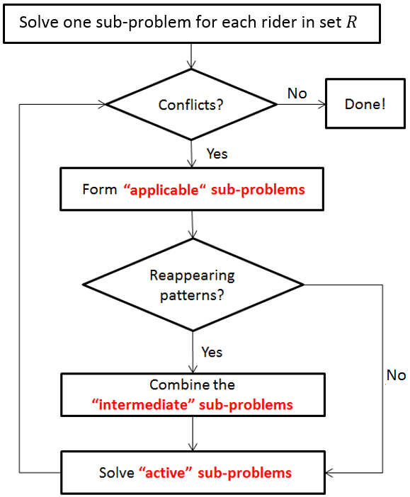
Figure 5: The decomposition algorithm flowchart

Let $R_{i}^{k}$ and $D_{i}^{k}$ denote the set of riders and drivers in sub-problem $k$ of iteration $i$, respectively. Each sub-problem includes a subset of riders in the problem. Once the subset of riders for sub-problem $k$ in iteration $i$ is determined, the set of drivers can be formed as $D_{i}^{k}=\{d|\forall r\in R_{i}^{k},(r,d)\in M\}$.

The algorithm starts by solving $|R|$ sub-problems, each including one of the riders in set $R$. In the case of there being no conflicts between the solutions, the solution to the original problem is readily available. This happens if each rider is matched with a different driver, or if multiple riders are matched with the same driver and the driver is capable of performing all the pick-up and drop-off assignments for the assigned riders. If not, conflicts are identified. Note that existence of conflicts between drivers’ paths in different sub-problems implies that the union of solutions to the sub-problems is infeasible to the original ride-matching problem.

In each iteration, in the case of there being conflicts between solutions of the sub-problems in the previous iteration, we form the set of “applicable” sub-problems. An “applicable” sub-problem is comprised of: $(i)$ sub-problems from the previous iteration from which riders have been excluded (with the remaining set of riders), and $(ii)$ a group of riders from the last iteration’s sub-problems with identical driver assignment (if these assignments conflict in time or space). Note that in the latter case if there are multiple groups of riders with identical but conflicting driver assignments, any such groups can be selected to form the new sub-problem. Sub-problems in the previous iteration that are not applicable sub-problems will be carried out to the next iteration without any change.

After the new set of sub-problems are formed, first we have to check to see if there are any loops between iterations. If the set of sub-problems in the current iteration is similar to the set of sub-problems in a previous iteration, the algorithm will be looping between iterations if no measures are taken. To prevent this, we re-define sub-problems in the current iteration by forming an “intermediate” sub-problem whenever a loop is identified. An “intermediate” sub-problem combines the sub-problems from the previous iteration that contribute to the loop, and hence prevent it (refer to Algorithm 2 in Appendix B for details.)

After all the new sub-problems are determined, a decision has to be made on whether a sub-problem needs to be solved or not. Sub-problems that need to be solved are called “active” sub-problems. These sub-problems are the ones whose optimal solutions cannot be readily obtained from the previous solutions. Sub-problems that have already been solved in the previous iterations (such as non-applicable sub-problems) are not active. In addition, if a sub-problem is the union of multiple sub-problems in a previous iteration, and the solutions of these sub-problems do not conflict, the solution to the sub-problem can be readily obtained by combining the solutions of the non-conflicting sub-problems. The algorithm stops if the solutions to the current iteration’s sub-problems do not have any conflicts, i.e., each driver is assigned to one route only.

Note that using this decomposition algorithm, a large problem could be solved in the first iteration, or we might end up solving multiple sub-problems before having to solve the original problem in the last iteration. The main merit of this algorithm is that sub-problems in each iteration can be solved independently. This also indicates that parallel computing implementations are possible.

After performing the pre-processing procedure and while applying the decomposition algorithm, we use a refined version of the the optimization problem in model (10), presented in Appendix C. This refined problem (model 10) is very similar to model 5, with two major differences: (i) Constraint sets (5h) and (5o) are now redundant, since the requirement to not exceed the maximum ride time is met when we form the reduced graphs and perform the forward and backward movements in the pre-processing procedure, and (ii) input sets in model (10) are more refined owing to both the pre-processing procedure and the decomposition algorithm.

6.1 Illustrative Example

Assume that a ridesharing system has 6 riders and 4 drivers, and that all drivers have spatiotemporal proximity with all riders, i.e., $\forall\>(r,d)\in R\times D,\;(r,d)\in M$. The iterations of the decomposition algorithm are displayed in Figure 6. As the interest is in showing the nature of the creation of sub-problems, the actual network on which this problem is solved is left out. The active sub-problems during each iteration are displayed in blue in the figure. The sub-problems whose solutions do not change throughout the iterations of the algorithm are displayed in green.

In iteration 1, each rider constitutes an active sub-problem. The solutions show that riders 1, 3, and 6 all have driver 1 in their solution, but in conflicting paths. Therefore, an active sub-problem of $\{r_{1},r_{3},r_{6}\}$ is formed and solved in the second iteration. Also, since rider 2 was not able to find any matches even without facing competition from other riders, he/she will not be able to find a match in the current configuration of the system. Sub-problems $\{r_{4}\}$ and $\{r_{5}\}$ are not active sub-problems and their solutions are readily available.

The solution to the active sub-problem $\{r_{1},r_{3},r_{6}\}$ in iteration 2 indicates that the optimal matches for riders 5 and 6 are in conflict (they are both matched with driver 2, but through different paths.) So they form the applicable sub-problem $\{r_{5},r_{6}\}$. Also, since rider 6 was removed from the sub-problem $\{r_{1},r_{3},r_{6}\}$, the solution obtained for this sub-problem for riders 1 and 3 might not be optimal anymore. Therefore, a new applicable sub-problem $\{r_{1},r_{3}\}$ is formed. However, not both of these newly formed sub-problems are active. The optimal match for rider 5 is driver 2, and the optimal match for rider 6 is driver 1. Since these two do not have any conflicts, the solution to the $\{r_{5},r_{6}\}$ sub-problem is readily available.

The only active sub-problem in iteration 3 is $\{r_{1},r_{3}\}$. The solution to this sub-problem suggests that two new applicable sub-problems $\{r_{1},r_{3},r_{6}\}$ and $\{r_{5}\}$ need to be formed, which along with two sub-problems $\{r_{4}\}$ and $\{r_{2}\}$ should constitute the set of sub-problems for iteration 4. However, we had the exact same set of sub-problems iteration 2. Therefore, in order to avoid looping, a new (intermediate) sub-problem $\{r_{1},r_{3},r_{6},r_{5}\}$ is formed in iteration 4. After solving this sub-problem, we find that there are no more conflicts. Hence, the global solution to the original problem is obtained in iteration 4. A total of 9 sub-problems needed to be solved for this solution to be obtained. However, in iteration 1, all 6 active sub-problems could be solved simultaneously.

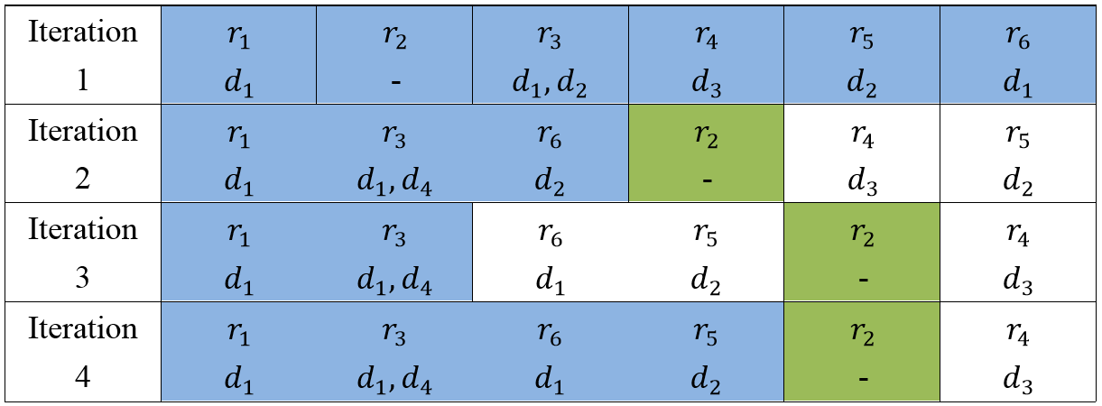
Figure 6: Iterations of the decomposition algorithm

It is possible to use a simpler version of the algorithm which is easier to implement, but may take longer to solve. In this simplified version, if any two riders in two sub-problems have conflicts, all the riders in the two sub-problems are combined into a new sub-problem in the following iteration. This will lead to potentially fewer iterations, but larger sub-problems to be solved in each iteration.

Let us apply this simplified algorithm to the example above. The sub-problems in each iteration are presented in Figure 7. Here, after solving the active sub-problem $\{r_{1},r_{3},r_{6}\}$ in iteration 2, and studying the solutions of all sub-problems, it turns out that riders 6 and 5 are both matched with driver 2, but through conflicting paths. Therefore, in the next iteration the two sub-problems $\{r_{1},r_{3},r_{6}\}$ and $\{r_{5}\}$ are combined. In this particular example, using the simplified version of the algorithm leads to reaching the optimal solution in fewer iterations, and less amount of time, since in Figure 7 we are skipping iteration 3 in Figure 6. Although reaching the optimal solution in fewer iterations is expected using the simplified version of the algorithm, a smaller solution time is not a typical behavior to be expected from the simplified version of the algorithm.

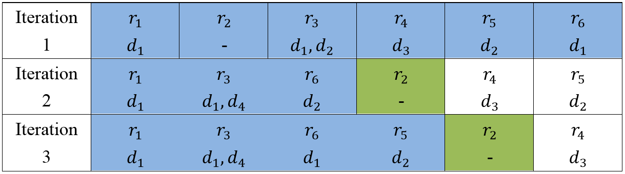
Figure 7: Iterations of the simplified decomposition algorithm

6.2 Properties of the Decomposition Algorithm

6.2.1 Optimality

During each iteration of the decomposition algorithm, we are in fact solving a relaxation of the original ride-matching problem. In the original optimization problem each driver can be assigned to a single route. By including a driver in multiple sub-problems, we might have the driver being routed differently in each. In fact, we are relaxing the constraint sets that force each driver to take a single route. Throughout the iterations, we are trying to find conflicts of this nature, and merge the sub-problems whose solutions demonstrate such a conflict, in an attempt to find a solution with no conflicts.

If the optimal solution to this relaxation satisfies the omitted set of constraints, then this solution would be optimal to the original problem as well. We have based the stopping criterion of our algorithm on this factual principle. After the final iteration of the algorithm, there exist no more conflicts between any given driver’s routes in different sub-problems. Therefore, what we find through the use of the decomposition algorithm is indeed an optimal solution to the relaxation of the original problem that does not violate the set of omitted constraints. Hence the solution found is the globally optimal solution to the original problem.

It should be noted that throughout the iterations, the union of the sub-problem solutions form an infeasible solution to the original problem. It is only in the last iteration, where there are no conflicts among driver assignments, when the first feasible solution is obtained, and this feasible solution is in fact the optimal solution. Furthermore, note that although the pre-processing procedure may eliminate some of the drivers from the pool of drivers available for each rider, it does not affect the optimality of the final matching. The omitted drivers could not have contributed to the solution in any case, since they did not have spatiotemporal proximity to the riders. Additionally, note that the proposed algorithm is optimal as long as maximizing the matching rate (or any rider-related terms, such as minimizing the total VMT by riders) remains the primary objective of the system. Otherwise, the decomposition algorithm provides a bound on the optimal solution.

6.2.2 Bounds

In this section we discuss computing upper and lower bounds on the optimal value of the optimization problem in model (5) after each iteration of the decomposition algorithm. We compute the bounds for the objective function in (5a), but the concept can be easily extended to a variety of objective functions.

Clearly, if a ride-matching problem is solved to optimality, the upper and lower bounds would be similar. However, if there is a time limit on reaching a solution, we might be obliged to settle for a sub-optimal solution (as will be described later in section 8.3). In that case, upper and lower bounds on the optimal solution can be computed after completion of each iteration to provide insight on the quality of the solution.

The main objective in model (5) is to find the maximum number of served riders, and the second term in (5a) has been added only for technical reasons (to ensure that the constraint sets work properly, as explained in Proposition 1 in Appendix A.) Therefore, while solving the sub-problems, we include this term, but use only the value of the first term as the value of the objective function of the problem while deriving bounds.

In section 6.2.1, we discussed that the solution reached in every iteration of the decomposition algorithm is infeasible, until the last iteration. This infeasibility is caused by conflicts between itineraries of common drivers in different sub-problems. When such conflicts exist, the best case scenario is for all the riders who are receiving conflicting itineraries to be eventually served in the system. Therefore, the upper bound in each iteration can be computed as the sum of the number of served riders in all sub-problems, regardless of the conflicting driver itineraries. It should be noted that the upper bound is strictly non-increasing with the number of iterations. The reason is that when two sub-problems have conflicting assignments during a given iteration, the riders who are receiving conflicting itineraries will be included in the same sub-problem in the following iteration. If all such conflicting riders can be served, then the upper bound to the objective function does not change. Otherwise, the upper bound will decrease.

The lower bound in each iteration can be obtained by solving a set packing problem. The optimal solution to sub-problems of a typical iteration provides us with information on the riders with conflicting itineraries, and drivers who form the itineraries of such riders. To find the tightest lower bound, we have to find the maximum number of riders who could be served under the current configuration (i.e., assuming that the driver routes are fixed.) This is analogous to solving a set packing problem where the universe is the set of drivers, and the sub-sets are drivers who form each rider’s itinerary. It should be noted that unlike the upper bound that has a non-increasing trend with the number of iterations, the lower bound is not necessarily non-decreasing with iterations. In addition, note that the lower bound corresponds to a feasible solution, while the upper bound corresponds to a possibly infeasible solution. Figure 8 shows the lower and upper bounds for the example in section 6.1. Clearly the lower and upper bounds meet at the final iteration.

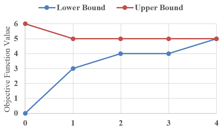
Figure 8: Bounds on the objective function value for the example in section 6.1

As we mentioned in the beginning of this section, we can follow a similar logic to compute bounds for a variety of objective functions, as long as serving the maximum number of riders remains the primary objective of the system. Since we are solving a relaxation of the original ride-matching problem at each iteration, no matter the objective function, sum of the objective functions of sub-problems always provides an upper bound on the original problem. To obtain a lower bound at each iteration, similar to what we did for the objective function in (10a), we have to derive a feasible global assignment from the solutions of sub-problems at each iteration by solving a set packing problem. At each iteration, once we find the set of riders who can be served, the drivers who serve them and the itineraries of these riders and drivers are readily available, and can be used to calculate any measures that are included in the objective function to obtain a lower bound.

7 Numerical Study

To evaluate the performance of the proposed decomposition algorithm, we generate and solve 420 random instances of the ride-matching problem. Each problem instance has a different size in terms of number of riders and drivers, and is generated in a grid networks with 49 stations. The results reported here are averaged over 10 runs for each problem instance.

The number of participants $|P|$ in the problem instances varies between 20 and 400, and the number of riders $|R|$ between 1 and $|P|$. Origins and destinations of trips are selected uniformly at random among the 49 stations. Earliest departure times of all trips are generated randomly within a one hour time period. The maximum ride time for a participant $p$ is generated randomly based on a “travel time budget factor” of 1.1, indicating that the particpant’s maximum ride time takes a value within the window $[tt_{(OS_{p},DS_{p})},1.1\thinspace tt_{(OS_{p},DS_{p})}]$, where $tt_{s_{1},s_{2}}$ is the travel time between stations $s_{1}$ and $s_{2}$. The latest arrival times are simply the sum of the earliest departure times and the maximum ride times of participants. Each vehicle is assumed to have 4 empty seats, and each rider is assumed to accept up to three transfers.

The ride-matching instances are solved on a PC with Core i7 3 GHz and 8GB of RAM. The optimization problems are coded in AMPL, and solved using CPLEX 12.6.00 with standard tuning.

In addition to solving the 420 problem instances with the stated default parameter values, we solve additional problem instances in the following sections to conduct sensitivity analysis over some of the parameters of the problem, including the number of stations, the spatiotemporal proximity of trips, and the maximum ride times of participants. The parameter values used in the rest of the paper are the default values, unless otherwise specified. Furthermore, the results presented in the rest of the paper are for solving the static versions of problems, unless otherwise specified.

7.1 Pre-processing

In this section we look at the running time of the pre-processing procedure, and examine its impact on the size of the ride-matching problem that needs to be solved. Figure 9a shows the contour plot of the pre-processing time as a function of the size of the problem. The pre-processing time is the sum of two components: the time required to generate the set of feasible links for each participant, and the time required to find the set of feasible drivers for each rider. The former component consists of the time spent on generating reduced graphs, and forming sets of feasible links for participants using forward and backward movements. This task can be completed when a participant registers a request in the system, and hence is not a bottleneck when it comes to solving the ride-matching problem in real-time in a rolling time horizon implementation. Even if a large number of participants join the system at the same time, the computations can be done independently, and implemented in a parallel computing system.

The latter component of the pre-processing time consists of the time required to compare each rider’s set of feasible links to those of the drivers. Similar to the first component, these computations can be done once a rider joins the system (with all registered drivers), and updated continuously as drivers keep joining the system.

The total pre-processing time depends on the size of the problem. For the 420 problem instances solved in this section, the maximum time was 3.5 seconds. The distribution of the pre-processing times over the range of sizes of the randomly generated instances are displayed in Figure 9a. The pre-processing procedure managed to reduce the average size of the link sets for participants to $0.01$ of the size of the original link set $L$.

Not only does the pre-processing procedure lead to indirect savings in solution times by limiting the size of the input sets to the optimization problem, but more importantly a quick scan of the participants’ feasible links can lead to direct and more considerable savings in solution times. For a rider to be served, he/she should have spatiotemporal proximity with at least one driver at both origin and destination stations. Whether such proximity exists can be easily examined using the sets of feasible links. Riders who do not enjoy spatiotemporal proximity at both origin and destination stations can be filtered out from the system. Figure 9b shows the percentage of riders filtered out from each problem instance during the pre-processing procedure. This figure suggests that, for a given number of riders, the lower the number of drivers, the higher the number of filtered riders, as expected.

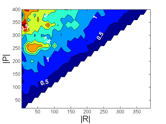
(a) Pre-processing time (sec)

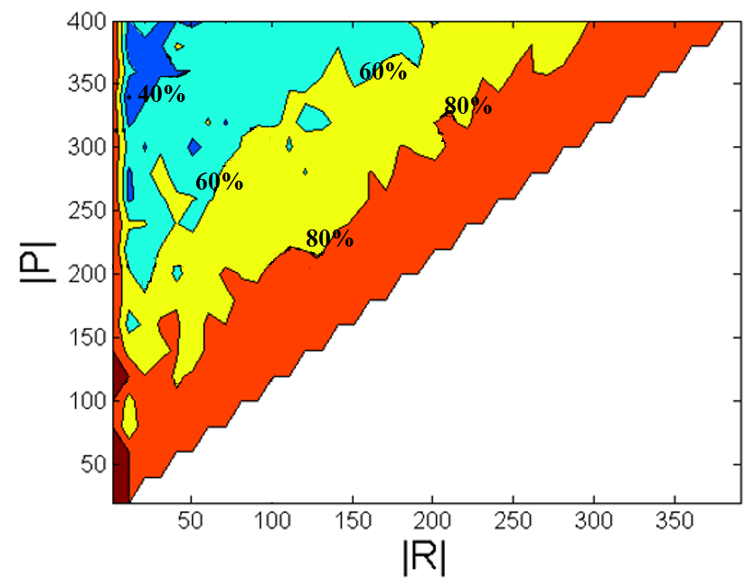
(b) Percentage of filtered riders

Figure 9: The pre-processing procedure

7.2 Value of a Multi-hop Solution

A ridesharing system can use a variety of approaches to match riders with drivers. Ride-matching methods could differ in multiple aspects, ranging from the flexibility in routing of drivers, to the type of routes devised for riders (single- or multi-hop). Matching methods can be formulated as optimization problems, and solved to optimality. However, different ride-matching methods lead to different system performance levels.

In this section, in order to investigate the effectiveness of the ridesharing system defined in this study, we compare its performance with a few more common ride-matching methods. Figure 10 compares the cumulative number of served riders in the 420 randomly-generated problem instances using five different matching methods. The problem instances in this figure are sorted by the number of participants.

The first matching method labeled as the “OD-based” in Figure 10 matches riders and drivers who share the same origin and destination locations, if their travel time windows allow. The second matching method, labeled as “Single-hop, Fixed-route” matches each rider with a single driver, where the drivers’ routes are pre-specified and fixed (although they still have flexibility in departure time.) The third matching method labeled as “Multi-hop, Fixed-route” allows riders to transfer between drivers. The drivers’ routes, however, remain pre-specified. The fourth matching method labeled as “Single-hop, Flexible-route” matches each rider with one driver only. In this method, however, the ridesharing system takes over routing of the drivers. The fifth and final matching method labeled as “Multi-hop, Flexible-route” allows riders to transfer between drivers. The driver routes are not pre-specified, and will be determined by the system.

As Figure 10 indicates, the “OD-based” matching method provides the least number of matches. The “Single-hop, Fixed-route” method does significantly better, since using this method not only can drivers carry the riders who share the same origin and destination locations with them (as in the “OD-based” method), but also they can carry passengers whose origin and destination locations lie on their pre-specified routes. The “Multi-hop, Fixed-route” matching method produces results that are slightly superior to the “Single-hop, Fixed-route” method, implying that allowing riders to transfer between drivers is in general beneficial to the system.

The “Single-hop, Flexible-route” and “Multi-hop, Flexible-route” methods lead to considerable improvements in the number of matches. This implies that having the system route drivers can be one of the most influential features of a ridesharing system. Comparison of the “Single-hop, Flexible-route” and “Multi-hop, Flexible-route” methods suggests that allowing transfers in the system is the second most important factor, after routing drivers. In addition, comparing the “Single-hop, Flexible-route” and “Multi-hop, Flexible-route” methods with “Single-hop, Fixed-route” and “Multi-hop, Fixed-route” methods suggests that the value of a multi-hop solution becomes more prominent when the driver routes are not pre-specified.

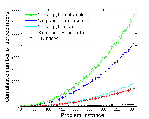
Figure 10: Cumulative number of served riders using five different matching algorithms

Figure 10 measures the efficiency of the matching methods based on the number of served riders. What this figure fails to demonstrate is how measures of quality of service, such as number of transfers and waiting times in transfer stations for riders, and the average vehicle occupancy and the extra time spent in the network by drivers compare between these methods. Table 1 displays these measures of quality of service along with some additional metrics to assess the five matching methods from different perspectives.

The results presented in this table are averaged over 10 runs with 400 participants, 200 of which are drivers and 200 are riders. This problem configuration is selected because it yields the highest number of served riders, regardless of the matching method. The earliest departure times of all trips are randomly generated within a 60 minute time period, and the trip origin and destination stations are selected randomly among the 49 stations. The quality of service measures in this table are averaged over all participants in all randomly-generated problems.

Table 1 suggests that in addition to serving higher number of riders, the multi-hop matching methods also engage higher number of drivers, compared to their single-hop counterparts. Although the ultimate purpose of a ridesharing system is serving riders, involving higher number of drivers is important as well, because users who do not get matched might stop registering in the system after a few failed attempts. Another interesting point is that in multi-hop matching methods the number of matched drivers is higher than the number of served riders. In spite of this observation, the average number of riders a driver in a multi-hop system carries is slightly higher than the average number of riders carried by a driver in a single-hop system.

Another interesting observation is that vehicle occupancies are highest in a multi-hop fixed-route system. In such a system, because driver’s routes are fixed, a smaller percentage of drivers get matched. However, drivers who get matched are the ones who drive on “popular” routes, and therefore end up with higher occupancy rates. In other words, although the system is not routing drivers, those drivers who try to optimally route themselves will benefit more compared to the case where the system routes all drivers.

Table 1 suggests that the measures of quality of service stay within reasonable ranges for all matching methods. It should be noted, however, that these measures correlate with the problem parameters in general, and are more sensitive to some parameters than others, as we will see in the following sections.

Table 1: Quality of service measures for the five matching methods in a system with relatively low spatiotemporal proximity among trips

		Riders					Drivers
		Num. (%)	Min\avg.\max	Min\avg.\max		Num. (%)	Min\avg.\max	Min\avg.\max
Matching method		served	num. transfers	wait in transfer (min)		involved	extra travel time (min)	riders on board
OD-based		5 (3%)	NA	NA		5 (3%)	NA	1.0\1.0\1.0
Single-hop, Fixed-route		11 (6%)	NA	NA		8 (4%)	NA	1.0\1.4\3.1
Multi-hop, Fixed-route		16 (8%)	0.0\0.6\1.9	0.0\0.4\2.5		18 (9%)	NA	1.0\1.4\3.2
Single-hop, Flexible-route		32 (16%)	NA	NA		26(13%)	0.0\3.0\8.1	1.0\1.2\2.3
Multi-hop, Flexible-route		52 (26%)	0.0\0.5\2.6	0.0\0.6\2.1		62(31%)	0.0\2.1\6.9	1.0\1.3\1.8

Table 2: Quality of service measures for the five matching methods in a system with relatively high spatiotemporal proximity among trips

		Riders					Drivers
		Num. (%)	Min\avg.\max	Min\avg.\max		Num. (%)	Min\avg.\max	Min\avg.\max
Matching method		served	num. transfers	wait in transfer (min)		involved	extra travel time (min)	riders on board
OD-based		21(11%)	NA	NA		19(10%)	NA	1.0\1.1\2.4
Single-hop, Fixed-route		79(40%)	NA	NA		62(31%)	NA	1.0\1.3\4.2
Multi-hop, Fixed-route		89(45%)	0.0\1.5\2.5	0.0\0.9\3		104(52%)	NA	1.0\1.9\3.1
Single-hop, Flexible-route		104(52%)	NA	NA		79(35%)	0.0\2.5\6.1	1.0\1.3\2.9
Multi-hop, Flexible-route		152(76%)	0.0\2.2\2.9	0.0\1.3\5		181(86%)	0.0\4.7\8.8	1.0\1.3\3.6

The problem instances whose performance we studied in Table 1 represent a ridesharing system that is spatiotemporally sparse. To compare the matching methods in a more realistic setting, we generated 10 random instances of a ridesharing system with higher spatiotemporal proximity among trips (Table 2). Similar to the problem instance studied in Table 1, this problem instance contains 400 participants, 200 of which are riders and 200 are drivers. The earliest departure times of all trips is generated within a 30 minute time period. The network is clustered into two sets of non-intersecting sections, where all trip origins are randomly selected from stations located in one of the sections, and all trip destinations from the other. This trip generation procedure significantly increases the spatiotemporal proximity among trips. The number of served riders and matched drivers using all five ride-matching methods along with some measures of quality of service are demonstrated in Table 2. This table suggests that all matching methods serve higher number of riders in a more spatiotemporally-dense ridesharing system.

7.3 Percentage of Satisfied Riders’ Requests

Figure 11 displays the contour plots of the percentage of satisfied riders for the 420 randomly generated problem instances. As intuition suggests, for a given number of riders, the percentage of served requests increases with the number of drivers in the system. Analyzing this type of graph can be especially helpful when one is interested in the critical mass of participants required to keep the system up and running, or when looking to set marketing strategies. For example, if we have 100 registered riders in a network where the origin and destination of trips are completely random, and aim to serve at least 40% of the unfiltered riders, then we know we need at least 230 drivers (330 participants), and can tailor our marketing strategies accordingly.

Note that the percentages shown in Figure 11 are the result of uniformly distributed OD patterns in the problem instances, which is the worst case scenario with a much less chance of joint rides than found in real networks, where trip distributions imply high demands for certain OD pairs, hence increasing the spatial proximity of trips in the network. It is expected that real networks can operate with much better ratios between drivers and riders. As a consequence, marketing attempts in real networks can be targeted towards the more popular OD pairs.

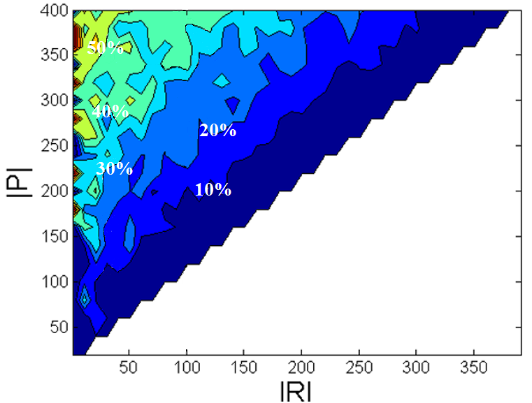
Figure 11: Percentage of un-filtered riders served

7.4 Algorithm Performance

Figures 12a and 12b compare the time required to solve the randomly generated ride-matching problems to optimality, without and with the decomposition algorithm, respectively. Solution times in these figures were obtained by solving models (5) and (10), respectively, using the CPLEX optimization engine. Comparison of these two figures suggests considerable savings in solution times can be obtained using the decomposition algorithm, without any trade-offs in terms of solution accuracy. Note that solution times reported in Figures 12a and 12b have been obtained for solving the optimization problems after applying the pre-processing procedure. The majority of the raw versions of the 420 problem instances cannot be solved without reducing the size of the problem instances (will run out of memory.)

Figure 13 shows the number of iterations of the decomposition algorithm it takes to solve the problems to optimality. Note that the higher numbers of iterations correspond to problems with higher solution times. None of the problem instances require more than 7 iterations to be solved to optimality using the decomposition algorithm.

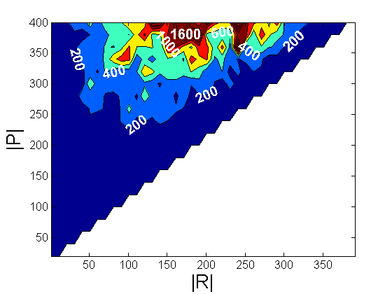
(a) Original matching problem solution times (sec)

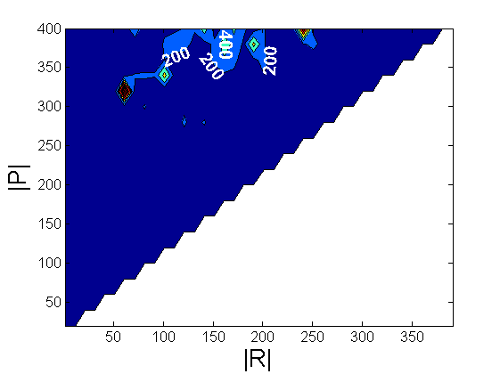
(b) Decomposition algorithm solution times (sec)

Figure 12: Improvements in solution times. Contour plots of solution times in seconds.

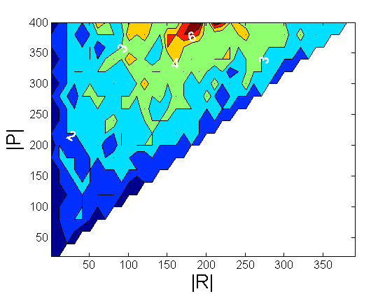
Figure 13: Number of decomposition algorithm iterations

7.5 Transfers

Transfers usually connote discomfort, and understandably so; since public transportation commonly runs under a fixed schedule, transit users might have to experience longer travel times and endure high waiting times in transfers. Note, however, that ridesharing systems of the future could be fundamentally different in nature, and better user-acceptance of transfers is possible depending on the ease of transfers, coordination of transfers in time, and reduction in transfer times offered by such systems (Taylor et al., 2009). This will naturally depend on the market penetration of the system as well as user-side behavioral changes, which are out of the scope of this paper. While this remains speculative, in this study we allow riders to specify their maximum number of transfers, and incorporate the maximum ride times requested by riders and drivers in our models. These input parameters could vary among individuals depending on their accessibility to personal vehicles, and their values of time. As an individual riders’ own transfer preferences are incorporated, this will help ease concerns on the perceived quality of service being affected by transfers.

A further reason to model a multi-hop ridesharing system is to a provide a general framework that can combine ridesharing systems with other modes of transportation, as discussed in section 2. It is straight-forward to include, say, a transit system simply as a set of high-capacity “drivers” with fixed routes in the formulation. In such cases, more than one transfer between the transit system and the rideshare mode is reasonable (one transfer from the rideshare vehicle to transit, and a second one from the final transit station to the rideshare vehicle.) Such multi-modal applications highlight the need for algorithms that do not systemically limit the number of transfers.

Figure 14 shows the cumulative distribution of number of transfers in the 420 problem instances solved in this section. Even though in our numerical experiments we assume that riders are comfortable with up to 3 transfers, this figure suggests that a considerable portion of trips can be served with zero to one transfer, and riders in over 90% of the problem instances can be fully served with no more than two transfers, which has serious implications when it comes to implementing a ridesharing system. This figure also suggests that transfers become necessary when the number of drivers is relatively low compared to the number of riders, as intuition suggests.

(a) Percentage of served riders with zero transfers

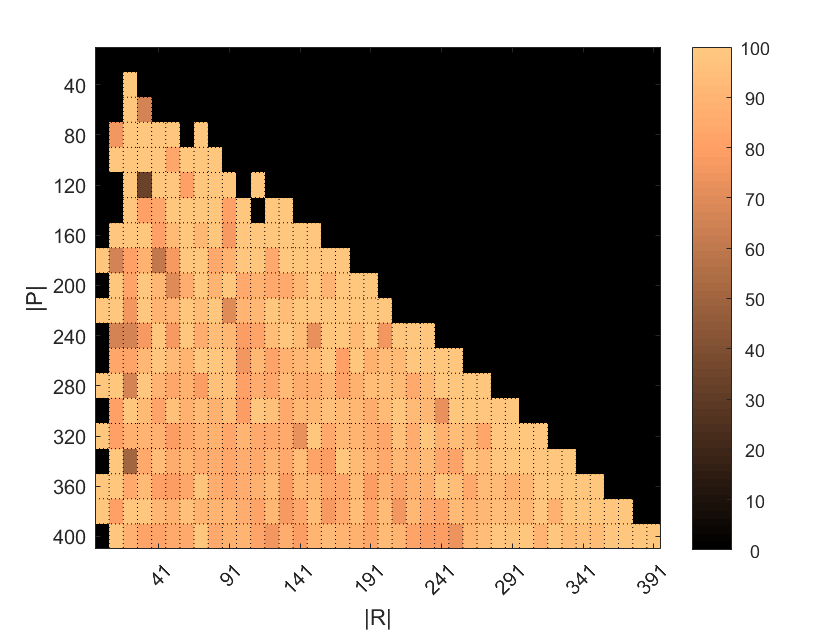
(b) Percentage of served riders with one or fewer transfers

(c) Percentage of served riders with two or fewer transfers

(d) Percentage of served riders with three or fewer transfers

Figure 14: Distribution of transfers

7.6 Sensitivity Analysis

In order to perform sensitivity analysis over some of the parameters of the ride-matching problem, we generate and solve two additional series of matching problems. All these problems contain 400 participants, with equal number of riders and drivers. This configuration is selected because Figures 11 and 12 suggest that problems with equal number of riders and drivers produce the highest number of matches and require the most computational resources. For the following problems, we maximize an objective function that includes two main terms: sum of the total number of served riders, ($\sum_{r\in R}z_{r}$), and sum of the weighted travel times by riders, $(-\sum_{r\in R}W_{r}\sum_{d\in D:(r,d)\in M}\sum_{\ell=(t_{i},s_{i},t_{j},s_{j})\in L_{rd}}(t_{j}-t_{i})y_{\ell}^{rd})$. The term $W_{r}=1/(T_{r}^{TB}+1)$ (where $T_{r}^{TB}$ is the maximum ride time for rider $r$) is considered as the weight for the travel time of rider $r$ in this objective function to ensure that maximizing the total number of served riders remains the main priority of the system. In the extreme scenario under which all riders use their entire travel time budget, this term ensures that the expression $\sum_{r\in R}W_{r}\sum_{d\in D:(r,d)\in M}\sum_{\ell=(t_{i},s_{i},t_{j},s_{j})\in L_{rd}}(t_{j}-t_{i})y_{\ell}^{rd}$ remains less than $1$, prioritizing the objective of maximizing the total number of served riders.

Table 3 shows the performance of the decomposition algorithm in solving 5 problem instances in a network with 49 stations. The field “release period” in this table indicates the period of time during which the earliest departure times of participants are generated. For this field, we used two values of 30 and 60 minutes. Problem instances with release period of 30 minutes incorporate higher temporal proximity between trips.

The field “Dir. trips” in Table 3 has a binary value. Value of zero for this field is used when the trip origin and destination locations are generated randomly in the network. In problem instances with value of 1 for this field, we use a clustered network. In a clustered network, trips experience a higher degree of spatial proximity.

Finally, we used two values of 1.1 and 1.2 as participants’ travel time budget factors to represent their flexibility on how much time they are willing to spend in the network. Value of 1.1/1.2 for this parameter indicates that all participants are assumed to have maximum ride times that are 1.1/1.2 times their shortest path travel times.

The field “Optimal” in Table 3 indicates whether a problem was solved to optimality (Y), or we ran out of memory when solving at least one of the sub-problems (the original problem in case of a static problem), and had to report the solution obtained by the heuristic described in section 8.3.

All these problem instances have been solved as both static problems, and dynamic problems with different re-optimization periods. For each problem instance, “NA” under the “Re-optimization period” indicates that the problem is solved in a static setting, assuming all participants to have registered their trips before the onset of the planning horizon when the matching problem is solved. Other values under this field show the re-optimization period. We assume that the entire demand for the re-optimization period $i$ arrives within the window $[(i-1)k,ik]$, where $k$ is the length of the re-optimization period. In addition, after each re-optimization period, we fix the itineraries of all matched riders and drivers, and include the fixed itineraries of matched drivers in the problems solved for the following re-optimization periods, if their travel time windows allow.

Not surprisingly, static versions of all five problem instances have the highest matching rates and the largest solution times compared to their dynamic counterparts, since static problems include all participants. Following the same logic, given a fixed number of participants, longer re-optimization periods translate into a larger pool of participants in the matching problems, and higher matching rates.

For each problem, we provide statistics on the number of rider transfers (based on the itineraries of matched riders), and the waiting time of riders during transfers (based on the itineraries of riders who experience transfers.) As a general trend, all these values decrease with the length of the re-optimization period, although the average waiting time of riders during transfers is in general negligible, especially given the potential uncertainties in travel times.

Table 3 also reports the number of matched drivers, and the statistics on the extra travel time by the matched drivers (compared to their shortest path travel times.) This table suggests that the number of matched drivers decreases with the length of the re-optimization period. However, no monotonic relationship can be observed between the drivers’ extra time in the network and the length of the re-optimization period.

Compared to the first problem instance, problem instances 4, 5, and 6 incorporate higher temporal, spatial, and spatiotemporal proximity among trips, respectively. Although all these problem instances lead to higher number of served riders compared to the first problem instance, it is interesting to note that the effect of higher spatial proximity on the number of served riders is more significant than that of higher temporal proximity. An interesting point to notice is that at 5-min re-optimization periods, all the problem instances can be solved in less than 1 minute.

The highest number of served riders is obtained in problem instance 2, where the participants’ time budgets is the highest. However, notice that the measures of quality of service, namely the average extra travel time for drivers, and the average number of transfers and transfer wait time for riders, are also considerably higher compared to other problem instances. The matching rate and quality of service measures reported on problem instance 3 in which riders are (naturally) assumed to have a higher maximum ride time than drivers lie between those of instances 1 and 2.

Table 4 displays problem instances similar to the ones in Table 3 in terms of problem parameters, but in a network with 100 stations. We should point out that we could not solve the static version of problem instance 5 to optimality (ran out of memory), and instead used the heuristic approach described in section 8.3. The two numbers reported under the “Num. served” field show the lower and upper bounds on the optimal solution (the lower bound solution is the feasible solution that can be eventually used). Note that if such a problem is encountered by a system due to lack of computational capacity, they could opt for re-optimizing the system more periodically.

In general, Table 4 demonstrates the same trends as in Table 3. The most prominent difference that can be observed comparing the two tables is that Table 4 has fewer number of served riders. This is an expected result, since by increasing the number of stations and keeping the same number of participants, we are in fact decreasing the spatial proximity among trips. In practice, however, increased number of stations could lead to potentially higher levels of demand, as higher number of stations translates into higher accessibility to the ridesharing system.

Table 3: Sensitivity study over the problem parameters. All instances are generated with 400 participants composing of 200 riders and 200 drivers in a randomly generated network with 49 stations

					Riders				Drivers			Solution
Problem	Dir.	Release	Time budget	Re-optimization	Num.	Min\avg.\max	Min\avg.\max		Num.	Min\avg.\max		time	Optimal
Instance	trips	period	rider/driver	period	served	num. transfers	wait in transfer		Involved	extra time		(sec)	Y/LB
				(min)			(min)			(min)
$1$	$0$	$60$	$1.1/1.1$	NA	69	0.0\0.9\3.0	0.0\0.6\3.0		98	1.0\2.7\3.0		518	Y
$1$	$0$	$60$	$1.1/1.1$	$10$	27	0.2\0.5\1.0	0.0\0.3\1.8		44	1.8\3.0\3.4		16	Y
$1$	$0$	$60$	$1.1/1.1$	$5$	20	0.4\0.4\0.8	0.0\0.4\1.2		36	1.1\2.2\3.2		6	Y
$2$	$0$	$60$	$1.2/1.2$	NA	150	0.0\2.1\2.1	0.0\2.5\4.1		144	0.0\11.2\15		1920	Y
$2$	$0$	$60$	$1.2/1.2$	$10$	72	0.0\0.6\1.7	0.0\1.3\3.1		105	2.9\8.5\11		174	Y
$2$	$0$	$60$	$1.2/1.2$	$5$	67	0.0\0.4\1.7	0.0\0.4\3.3		87	3.6\6.5\9.2		29	Y
$3$	$0$	$60$	$1.2/1.1$	NA	112	0.0\0.7\2.4	0.0\1.5\3.1		123	0.1\3.1\5.4		718	Y
$3$	$0$	$60$	$1.2/1.1$	$10$	43	0.0\0.4\1.2	0.0\0.8\3.0		80	2.0\3.0\5.1		53	Y
$3$	$0$	$60$	$1.2/1.1$	$5$	38	0.0\0.4\0.9	0.0\0.4\2.1		67	2.6\4.2\4.2		11	Y
$4$	$0$	$30$	$1.1/1.1$	NA	87	0.0\0.9\30	0.0\0.7\1.5		115	0.75\2.3\3.3		2357	Y
$4$	$0$	$30$	$1.1/1.1$	$10$	54	0.0\0.7\2.3	0.0\0.6\3.3		80	1.7\3.1\4.2		201	Y
$4$	$0$	$30$	$1.1/1.1$	$5$	48	0.0\0.4\1.5	0.0\0.5\3.7		68	0.5\2.5\4.3		12	Y
$5$	$1$	$60$	$1.1/1.1$	NA	137	0.0\2.1\3.0	0.0\1.7\7.0		158	0.0\2.4\8.0		1104	Y
$5$	$1$	$60$	$1.1/1.1$	$10$	73	0.0\0.8\2.3	0.0\0.6\2.8		107	0.0\2.4\7.06		52	Y
$5$	$1$	$60$	$1.1/1.1$	$5$	57	0.0\0.6\1.7	0.0\0.6\1.8		85	0.3\3.0\3.4		22	Y
$6$	$1$	$30$	$1.1/1.1$	NA	152	0.0\2.2\3.0	0.0\1.3\8.0		192	0.0\2.3\8.0		2750	Y
$6$	$1$	$30$	$1.1/1.1$	$10$	116	0.0\0.8\2.6	0.0\0.5\3.7		133	0.0\2.5\8.0		142	Y
$6$	$1$	$30$	$1.1/1.1$	$5$	101	0.0\0.6\1.5	0.0\0.4\2.2		112	0.1\1.9\6.2		48	Y

Table 4: Sensitivity study over the problem parameters. All instances are generated with 400 participants composing of 200 riders and 200 drivers in a randomly generated network with 100 stations

					Riders				Drivers			Solution
Problem	Dir.	Release	Time budget	Re-optimization	Num.	Min\avg.\max	Min\avg.\max		Num.	Min\avg.\max		time	Optimal
Instance	trips	period	rider/driver	period	served	num. transfers	wait in transfer		Involved	extra time		(sec)	Y/LB
				(min)			(min)			(min)
$1$	$0$	$60$	$1.1/1.1$	NA	61	0.0\1.8\2.7	0.0\1.8\10		94	0.0\4.4\7.0		501	Y
$1$	$0$	$60$	$1.1/1.1$	$10$	18	0.5\1.1\1.8	0.2\1.1\3.7		39	0.5\5.9\9.1		40	Y
$1$	$0$	$60$	$1.1/1.1$	$5$	11	0.3\0.5\0.7	0.1\0.4\0.8		20	0.3\3.9\8.2		36	Y
$2$	$0$	$60$	$1.2/1.2$	NA	138	0.0\2.4\2.5	0.3\2.4\6.2		124	0.0\16.2\20.2		1339	Y
$2$	$0$	$60$	$1.2/1.2$	$10$	59	0.1\1.6\2.1	0.0\1.0\5.1		83	1.0\14.3\19.8		515	Y
$2$	$0$	$60$	$1.2/1.2$	$5$	39	0.0\0.4\0.9	0.1\0.9\3.9		63	2.1\12.2\18.2		316	Y
$2$	$0$	$60$	$1.2/1.2$	$2$	32	0.0\0.3\0.6	0.0\0.7\3.1		40	0.1\8.1\14.0		115	Y
$3$	$0$	$60$	$1.1/1.2$	NA	85	0.1\1.8\2.5	0.3\2.1\4.1		102	0.0\2.1\6.2		1020	Y
$3$	$0$	$60$	$1.1/1.2$	$10$	35	0.3\1.5\1.9	0.1\1.2\4.0		49	0.2\3.9\7.1		180	Y
$3$	$0$	$60$	$1.1/1.2$	$5$	21	0.2\0.4\1.1	0.1\0.8\3.8		30	0.1\3.9\7.3		115	Y
$4$	$0$	$30$	$1.1/1.1$	$2$	36	0.2\1.0\1.5	0.2\0.8\2.0		63	0.1\4.5\8.2		866	Y
$4$	$0$	$30$	$1.1/1.1$	$10$	23	0.1\0.8\1.7	0.3\1.7\3.4		42	0.1\4.1\9.1		339	Y
$4$	$0$	$30$	$1.1/1.1$	$5$	15	0.0\0.4\0.7	0.3\0.7\2.3		23	0.1\3.2\7.6		31	Y
$5$	$1$	$60$	$1.1/1.1$	NA	132	0.5\2.4\2.9	0.4\1.9\4.1		145	0.0\6.7\8.9		856	Y
$5$	$1$	$60$	$1.1/1.1$	$10$	29	0.1\0.8\1.2	0.0\0.7\2.1		49	0.1\4.0\7.1		124	Y
$5$	$1$	$60$	$1.1/1.1$	$5$	19	0.1\0.7\0.9	0.1\0.4\1.9		32	0.2\4.5\7.1		30	Y
$6$	$1$	$30$	$1.1/1.1$	NA	[78 128]	0.4\2.4\2.7	0.1\1.3\3.8		161	0.2\6.2\10.1		753	LB
$6$	$1$	$30$	$1.1/1.1$	$10$	61	0.1\1.0\1.2	0.1\1.0\2.1		99	0.3\4.9\6.9		2140	Y
$6$	$1$	$30$	$1.1/1.1$	$5$	40	0.1\0.8\1.2	0.1\0.8\1.9		64	0.1\2.7\4.5		447	Y
$6$	$1$	$30$	$1.1/1.1$	$2$	28	0.0\0.5\0.7	0.1\0.7\1.5		42	0.0\1.0\3.1		123	Y

7.6.1 Maximum Ride Time

Since drivers in a risharing system are traveling based on their own schedules, it is safe to assume that they are less likely to have significant travel time budget factors (i.e., the total time one is willing to spend in the network as a percentage of one’s shortest path travel time). Riders in a ridesharing system, on the other hand, are more likely to consider rather larger travel time budget factors due to their possible lack of access to a private vehicle and/or the low frequency and potentially longer travel times of public transportation. It is reasonable to assume that increasing the travel time budget factor of participants would improve the matching rate by allowing larger detours from one’s shortest path and more flexibility in one’s departure and arrival times, but it would at the same time increase solution times as a result of larger link sets in the optimization problem. Figure 15 demonstrates this trade-off.

All the problem instances in Figure 15 include 200 riders and 200 drivers. The travel time budget factor of 1.1 is considered for drivers, and the rest of the parameter values are the default values from section 7. Figure 15 suggests that as we increase the rider travel time budget factor, both the matching rate and solution time demonstrate an increasing trend. While solution times increase exponentially with riders’ travel time budget factor, the increase in the matching rate seems to have a higher rate initially, up to the travel budget factor of 1.3, after which the rate of increase in the matching rate decreases. This is due to the fact that drivers’ availabilty in the network is bounded by their rather small travel time budget factor of 1.1, and although increasing the riders’ travel time budget factor helps improve the matching rate to some degree, higher improvement in the matching rate can be obtained by increasing driver-hours spent in the network (e.g., if current drivers stay in the network for longer and/or more drivers join the system.)

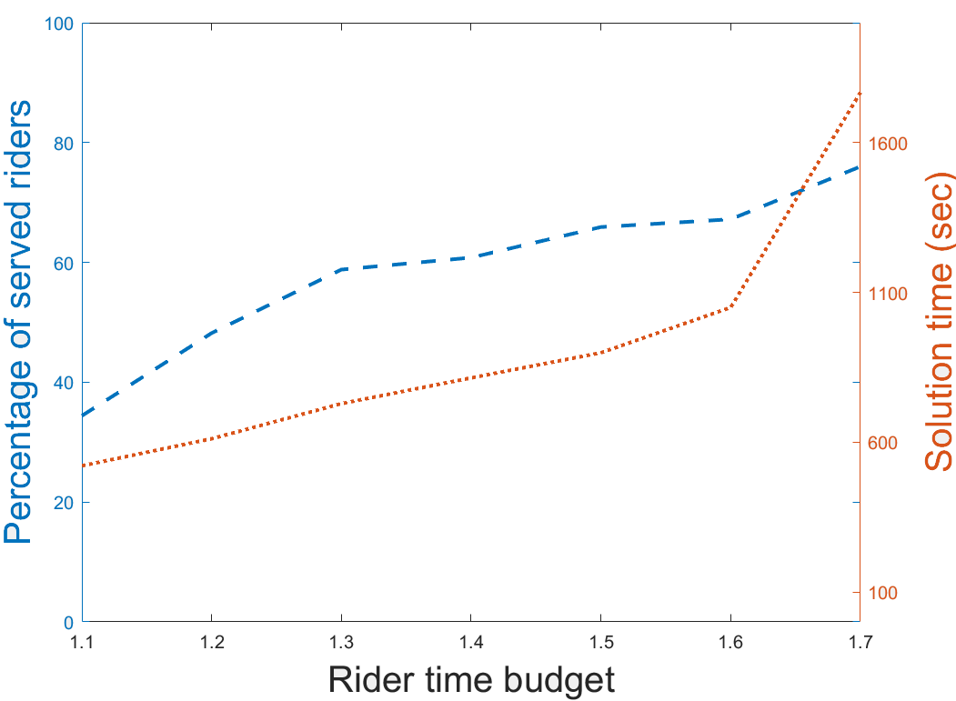
Figure 15: Impact of rider and driver maximum ride times on the matching rate and solution time

In the following section, we present methods to make the solution algorithm more appropriate for dynamic implementations by reducing the solution times even further.

8 Application in Practice

The scalability of the solution algorithm to solve the ride-matching problem may become an issue in practice. Larger area of coverage by ridesharing companies leads to larger number of stations, and potentially larger number of participants. Larger problems can lead to higher solution times and reduce the effectiveness of the proposed algorithm in dynamic applications.

Forming reduced graphs for participants can address this problem to a large extent. Even though a ridesharing company could cover a very large area, the distance traveled by participants is usually within a limited (but not necessarily small) circumference of their homes, i.e., within city limits, and therefore their reduced graphs contain a limited number of stations. It is only in rarer cases that people might require to, or be willing to, travel longer distances in a dynamic rideshare system. Thus it may be expected that larger reduced graphs would be rarer.

In order for the ridesharing system to cover longer (such as inter-city) trips, the system can locate one or two important stations in each city, and use only those set of stations for riders with long-distance trips. In addition, drivers who are selected to be included in the ride-matching problems with such riders can be limited to those who are making inter-city trips themselves. Using drivers with shorter trip lengths in such settings would not be practical due to the large number of transfers that forming an itinerary with short-distance drivers would require.

In the interest of lower solution times, in this section we suggest two different approaches to simplify the problem and obtain high quality heuristic solutions to the ride-matching problem within a reasonable time period.

8.1 Restricting the Number of Transfer Stations

In the ride-matching problem in model (5), itineraries are devised assuming transfers can occur at any station. In practice, we can identify stations where transfers are more likely to happen, and limit the set of transfer stations. Let us denote by $S_{T}$ the set of stations where transfers are allowed. The flow conservation constraint (5n) should then be replaced by two sets of constraints, (8) and (9). Constraint set (8) and (9) both model flow conservation. Constraint set (8) covers stations where transfers are allowed, and (9) covers the rest of the stations.

$$\!\!\!\sum_{{}^{d\in D^{\prime}}}\!\!\!\sum_{{}^{{}_{\ell=(t_{i},s_{i},t,s)\in L}^{\qquad t_{i},s_{i}:}}}\!\!\!\!\!y_{\ell}^{rd}=\sum_{{}^{\quad d\in D^{\prime}}}\!\!\!\sum_{{}^{{}_{\ell=(t,s,t_{j},s_{j})\in L}^{\qquad t_{j},s_{j}:}}}\!\!\!\!\!y_{\ell}^{rd}\quad\quad\begin{array}[]{l}\forall r\in R\\ \forall t\in T_{r}\\ \forall s\in S_{T}\backslash\{OS_{r}\cup DS_{r}\}\end{array}$$ (8)

$$\!\!\!\sum_{{}^{\>\>\>{}_{\ell=(t_{i},s_{i},t,s)\in L}^{\>\>\>\>\>\>\>\>\>t_{i},s_{i}:}}}\!\!\!\!\!y_{\ell}^{rd}=\!\!\!\sum_{{}^{{}_{\>\>\>\ell=(t,s,t_{j},s_{j})\in L}^{\>\>\>\>\>\>\>\>\>\>\>\>\>t_{j},s_{j}:}}}\!\!\!\!\!y_{\ell}^{rd}\quad\quad\quad\quad\qquad\qquad\begin{array}[]{l}\forall r\in R,\forall d\in D\\ \forall t\in T_{r}\\ \forall s\in S\backslash\{S_{T}\cup OS_{r}\cup DS_{r}\}\end{array}$$ (9)

To study the impact of limiting transfers to certain stations on the quality of the solutions and solution times, we experimented with the 420 randomly generated problem instances. For each problem instance, we studied the solution to model (5) where all stations are transfer stations, and identified the top 80% of stations where transfers occur. We then limited transfers to those stations only. Figure 16 shows the ratio of reduction in solution times (new solution times divided by the old solution times). The computational time reduction can range from 0 to 60%. It is interesting, however, to observe that the higher savings in solution times are obtained for problem instances with higher original solution times (see Figure 12a).

In terms of solution quality, number of served riders using the top 80% transfer stations remained on average within 95% of the number of served riders in the original solution, suggesting that the trade-off between the solution time and quality in dynamic settings may be in favor of restricting the number of transfer stations. These results are similar to the results found by Masson et al. (2014b). In their study of a multi-modal system designed to carry goods using a combination of excess bus capacities and city freighters, they found that 60% of the transfers took place in two bus stops that were closer to a large body of customers.

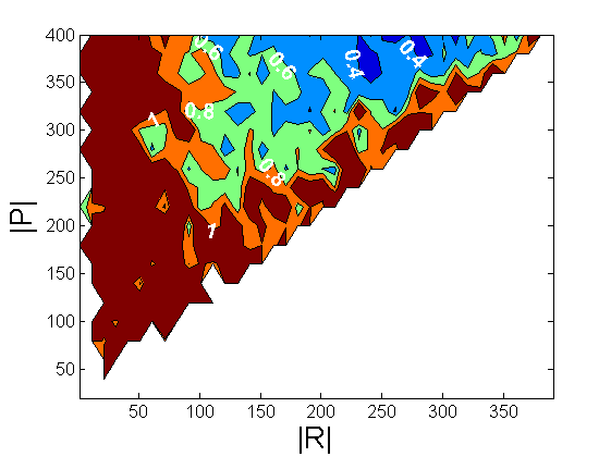
Figure 16: Ratio of new to old solution times after limiting the number of transfer stations

8.2 Selecting a time interval

In the numerical experiments in this paper, we discretized the study time horizon into 1-minute time intervals. In this section, we study the impact of using larger time intervals on the solution times, and discuss when using larger time intervals is appropriate.

The impact of using a larger time interval on solution times is not obvious without running experiments. On one hand, using a larger time interval will lead to smaller link sets produced by the pre-processing procedure. On the other hand, using a larger time interval causes a higher degree of temporal proximity among trips, which can lead to higher solution times. Figure 17 shows the solution times for the 420 randomly generated problems, solved using the decomposition algorithm with 5-minute time intervals. This figure suggests that utilizing larger time intervals leads to lower solution times. It should be noted that as participants’ maximum ride times become larger, so do the size of the link sets, and therefore the savings in solution times due to incorporating higher time intervals become more significant. Using larger time intervals, in addition to yielding lower solution times, can make it less probable for travel time uncertainties to cause individuals to miss their rides, especially during transfers.

Another issue that should be discussed is under what circumstances it is appropriate to use larger time intervals. In practice, individuals tend to report their schedules in five-minute increments at the finest, i.e., it is not typical to hear an individual planning to leave no later than 2:21 P.M., and therefore in general using larger time intervals (e.g., 5 min intervals) seems appropriate. For a ridesharing system that is integrated with a high-frequency transit system with minute-level time schedule, however, using smaller time intervals might be more suitable.

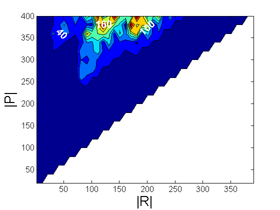
Figure 17: Solution times with 5-min time intervals

8.3 Heuristic solutions

In each iteration of the decomposition algorithm, a solution to the original ride-matching problem is available. In section 6.2.2, we saw that we can obtain a heuristic feasible solution in each iteration of the decomposition algorithm by solving a set packing problem. In this section we study the impact of stopping the decomposition algorithm at certain time limits and retrieving the best heuristic solution. The results are displayed in Figure 18.

Figure 18 suggests that the additional number of served riders obtained from allowing the computations to continue beyond 240 seconds is negligible. Comparing Figures 18 and 10 suggests that even at a computational cut-off time of 120 seconds, the number of served riders is higher than or comparable to the number of served riders in the other four ride-matching methods described in section 7.2. In fact, for several of the problems, even 60 seconds is sufficient. The fact that computations can be accomplished in a mere 2-minute period again validates the applicability of the optimizations schemes in dynamic settings.

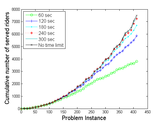
Figure 18: Quality of heuristic solutions

9 Conclusion

In this paper, we formulated the multi-hop P2P ride-matching problem as a binary program. The formulation has a very tight linear relaxation, and its structure limits the necessity for branching only to very specific cases. We proposed a pre-processing procedure to reduce the size of the input sets to this optimization problem, and an exact and finite decomposition algorithm to solve the problem by iteratively solving smaller sub-problems. Sub-problems in each iteration are independent of each other, making it possible for computations to be done in parallel. The computational savings achieved by the proposed algorithm can make it applicable for real-time applications. Furthermore, the fact that the proposed algorithm allows for as many transfers as necessary makes it suitable for use in multi-modal networks.

We conducted extensive numerical experiments to study the impact of multi-hop ridesharing on the number of served riders by comparing matching rates of five different matching algorithms with different degrees of flexibility. These experiments demonstrated the higher efficiency and throughput of a multi-hop ridesharing system. Another interesting observation was that the value of a multi-hop solution becomes more prominent when driver routes are determined by the system, and are not pre-specified. Furthermore, we conducted sensitivity study over different parameters, including the ratio of riders and drivers in the system, the spatiotemporal distribution of trips, and the maximum ride times requested by individuals.

We discussed different approaches, including clustering of trips in time and space and extracting heuristic solutions in each iteration of the algorithm, to make the proposed methodology applicable to dynamic, real-life sized problems. It is hoped that the algorithms presented and their variants will be applied in the near future to a variety of socially and economically beneficial ridesharing systems, and perhaps even to the scenarios of shared rides in automated or driverless vehicles that are further distant in the future.

Appendix A Proof of Proposition

Proposition 1.

Number of connections for rider $r$ can be calculated using term $\sum_{d\in D}u_{r}^{d}-1$.

Proof.

If driver $d$ carries rider $r$ on any link, then $u_{r}^{d}=1$. Therefore, the term $\sum_{d\in D}u_{r}^{d}-1$ provides the number of connections, only if a driver does not pick up a rider multiple times. Without loss of generality, we use the example in Figure 19 to show by contradiction that such a scenario cannot happen. Figure 19 shows a rider’s itinerary. On the first and third links, the rider is traveling with $d_{1}$, and on the second link, he/she is traveling with $d_{2}$. If $d_{1}$ travels on both $\ell_{1}$ and $\ell_{3}$, at some point $d_{1}$ must have traveled from node 2 to node 3, and the rider could have accompanied him on that ride too, reducing the number of transfers from 2 to 0. The term $-W_{r}\sum u_{r}^{d}$ in the maximization objective function ensures that the route with zero transfers is selected as the optimal solution. Alternatively, one could leave out this term from the objective function, and use post-processing to refine the solution. ∎

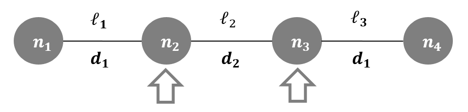
Figure 19: An undesirable match

Proposition 2.

(5v) and (5y) register all drivers who collectively form each rider’s itinerary.

Proof.

From (5v) we have $u_{r}^{d}\;\geq\;y_{\ell}^{rd}$. If $y_{\ell}^{rd}=1$, $u_{r}^{d}$ is forced to be 1. If $y_{\ell}^{rd}=0$, $u_{r}^{d}$ can take either 0 or 1. Constraint set (5y) ensures that in the latter case, $u_{r}^{d}$ takes its lower bound. ∎

Appendix B Decomposition Algorithm

We start the algorithm by setting the iteration counter, $i$, to 1 (line 2), and the sub-problem counter, $k$, to 0 (line 3). Each rider forms a new sub-problem in the first iteration of the algorithm, and the type of all sub-problems is set as active (lines 4-9). In Algorithm 2, $R_{i}^{k}$ denotes the set of riders in sub-problem $k$ of iteration $i$, and $SP_{i}$ denotes the set of sub-problems in iteration $i$. $Active(k)$ indicates whether the type of sub-problem $k$ is active (1) or not (0).

The second step of the algorithm involves solving the set of active sub-problems in the current iteration. We keep in set $D_{i}^{k}$ the list of all matched drivers in sub-problem $k$ of iteration $i$ (line 13), and in set $D_{i}$ the list of all drivers who have been matched in iteration $i$ (line 14). Furthermore, we use sets $Y_{i,k},$ $X_{i,k}^{d}$, and $Z_{i,k}^{r}$ to keep track of the itineraries of all riders, driver $d$ ($\forall d\in D)$, and whether rider $r$ $(\forall r\in R)$ has been matched in sub-problem $k$ of iteration $i$, respectively (lines 15-17).

In step 3 we check the stopping criterion of the algorithm. We start by setting the value of the indicator variable $Terminate(d)$ to zero (line 21). If driver $d$ is shown to have the same itinerary under all sub-problems, the value of the indicator variable $Terminate(d)$ will be set to 1 (lines 22-24). If the value of $Terminate(d)$ becomes 1 for all drivers, then the union of solutions to the sub-problems will yield the optimal solution to the original optimization problem $(X^{*})$ (lines 26-29).

Algorithm 2 The decomposition algorithm $01\quad$ Step 1. Initialize $02\quad$ $i\leftarrow 1$ $03\quad$ $k\leftarrow 0$ $04\quad$ For each rider $r\in R$ $05\quad$ $\qquad k\leftarrow k+1.$ $06\quad$       Set $R_{i}^{k}=\{r\}.$ $07\quad$       Set $Active(k)\leftarrow 1.$ $08\quad$ End For $09\quad$ Set $SP_{i}=\{1,...,|R|\}.$ $10\quad$ Step 2. Solve the (active) sub-problems $11\quad$ For each sub-problem $k\in SP_{i}$ for which $Active(k)=1$ $12\quad$       Solve sub-problem $k$. $13\quad$       Let $D_{i}^{k}=\{d\in D\;|\;\sum_{r\in R_{i}^{k},\ell\in L_{rd}}y{}_{\ell}^{rd*}\geq 1\}.$ $14\quad$       Let $D_{i}=\bigcup_{k\in SP_{i}}D_{i}^{k}.$ $15\quad$       Let $Y_{i,k}=\big{(}y{}_{\ell}^{rd*}\big{)}_{r\in R_{i}^{k},d\in D_{i}^{k},\ell\in L_{rd}}.$ $16\quad$       Let $X_{i,k}^{d}=\big{(}x_{\ell}^{d*}\big{)}_{\ell\in L_{d}},\;\forall d\in D_{i}^{k}.$ $17\quad$       Let $Z_{i,k}^{r}=z_{r}^{*},\;\forall r\in R_{i}^{k}.$ $18\quad$ End For $19\quad$ Step 3. Termination Criterion $20\quad$ For each driver $d\in D_{i}$ $21\quad\qquad Terminate(d)\leftarrow 0$. $22\quad$       If $X_{i,m}^{d}=X_{i,n}^{d}$ for all $(m,n)\in D_{i}^{m}\times D_{i}^{n}$ $23\quad$ $\qquad\qquad Terminate(d)\leftarrow 1.$ $24\quad$       End If $25\quad$ End For $26\quad$ If $\sum_{d\in D_{i}}Terminate(d)=|D|$ then $27\quad\qquad$ Stop. $28\quad$ Final optimal solution $X^{*}=U_{k\in SP_{i}}\big{(}Y_{i,j},\cup_{d\in D}X_{i,k}^{d},\cup_{r\in R}Z_{i,k}^{r}\big{)}$. $29\quad$ Else $30\quad$       Continue to Step 4. $31\quad$ End If

If the algorithm does not terminate in step 3, we move forward to step 4 to form the set of sub-problems for the next iteration (line 33). We start step 4 by defining set $R^{\prime}$ to include all riders that need to be allocated to sub-problems in the new iteration, and initialize it with $R$ (line 35). Next, we go through the list of matched drivers in the previous iteration (in no particular order). For each driver, we find the riders in set $R^{\prime}$ that have the driver on their itinerary. These riders (if belonging to different sub-problems) will from a new sub-problem in the current iteration (line 42), and are removed from set $R^{\prime}$ (line 43). We mark all such sub-problems $k$ as applicable by setting the value of indicator $Applicable(k)$ to 1 (line 43).

At this point, there could still be riders that do not belong to any sub-problems in the new iteration. Next, we go through the sub-problems from the previous iteration one by one (lines 47-58). For a given sub-problem $j$ from the previous iteration, we find all riders $r$ who do not belong to any sub-problems in the current iteration (i.e., $r\in R^{\prime}$). If such riders exist, they will from a new sub-problem in the current iteration. If it turns out that we are importing an entire sub-problem from the previous iteration to the current iteration, then this sub-problem does not need to be solved again, and so we set the applicability indicator of the sub-problem to zero (lines 49-51). Otherwise, if we are importing only a part of a sub-problem from the previous iteration as a new sub-problem to the current iteration, then the solution from the previous iteration is not necessarily optimal anymore, and so we set the applicability indicator of the new sub-problem to 1 (lines 53-55). We next move to Step 5.

Algorithm 2 (continued) The decomposition algorithm $32\quad$ Step 4. Form the set of sub-problems for the next iteration $33\quad$ $i\leftarrow i+1$ $34\quad$ $k\leftarrow 0$ $35\quad$ Let $R^{\prime}=R$. $36\quad$ For each driver $d\in D_{i-1}$ such that there are at least two sub-problems $(m,n)\in SP_{i-1}\times SP_{i-1}$ $37\quad$ with $d\in D_{i-1}^{m}$ and $d\in D_{i-1}^{n}$ $38\quad$       Let $R_{temp}=$ set of all riders $r\in R^{\prime}$ that have driver $d$ on their optimal path $39\quad$       in any sub-problems $k\in SP_{i-1}$. $40\quad$       If $R_{temp}\not=\emptyset$ then $41\quad$             Form a new sub-problem: $k\leftarrow k+1$. $42\quad$             Set $R_{i}^{k}=R_{temp}$. $43\quad$             Update $R^{\prime}\leftarrow R^{\prime}\backslash R_{temp}$. $44\quad$             Set $Applicable(k)\leftarrow 1$. $45\quad$       End If $46\quad$ End For $47\quad$ For $j\in SP_{i-1}$ $48\quad$       If $|R_{i-1}^{j}\cap R^{\prime}|=|R_{i-1}^{j}|$ then $49\quad$             Form a new sub-problem: $k\leftarrow k+1$. $50\quad$             Set $R_{i}^{k}=R_{i-1}^{j}$. $51\quad$             Set $Applicable(k)\leftarrow 0$. $52\quad$       Elseif $R_{i-1}^{j}\cap R^{\prime}\neq\emptyset$ and $|R_{i-1}^{j}\cap R^{\prime}|<|R_{i-1}^{j}|$ $53\quad$             Form a new sub-problem: $k\leftarrow k+1$. $54\quad$             Set $R_{i}^{k}=R_{i-1}^{j}\cap R^{\prime}$. $55\quad$             Set $Applicable(k)\leftarrow 1$. $56\quad$       End If $57\quad$ End For

In step 5, we prevent the algorithm from looping between iterations. After forming the set of sub-problems for the current iteration, we compare these sub-problems with sub-problems from previous iterations. If it turns out that two iterations have the exact same set of sub-problems, we form a new intermediate sub-problem in the current iteration by finding two sub-problems from the previous iteration such that each of these two sub-problems includes a subset of riders in a sub-problem in the current iteration (lines 62-63). These two sub-problems form a new sub-problem in the current iteration (line 64). Naturally, riders in this newly formed sub-problem are eliminated from their original sub-problems (line 65), and the newly formed intermediate sub-problem is marked as applicable (line 66).

The last step of the algorithm is to find the active sub-problems: those whose solutions cannot be derived from the solutions of previously solved sup-problems. There are two cases where sub-problems are not active: first, if the exact same sub-problem has been solved before, in which case the solution is readily available (lines 78-82); second, if a sub-problem $k$ is a union of a set of sub-problems from a previous iteration, and the solutions to these sub-problems do not have any conflicts in terms of itineraries of drivers. In this case, the solution to sub-problem $k$ would be the union of the solutions to this set of sub-problems (lines 87-90). Next, we go back to Step 2, where we solve the active sub-problems (line 96).

Algorithm 2 (continued) The decomposition algorithm $58\quad$ Step 5. Check for repeating patterns and form intermediate sub-problems $59\quad$ For $j\in 1$ to $i-2$ $60\quad$       If iterations $i$ and $j$ have the same set of sub-problems, then $61\quad$             For sub-problem $k\in SP_{i}$ $62\quad$                   Find two sub-problems $m,n\in SP_{i-1}$ such that they each share $63\quad$                   at least one rider with $R_{i}^{k}$. $64\quad$                   Add a sub-problem $k$ to $SP_{i}$ with combined set of riders $R_{i}^{m}\cup R_{i}^{n}$. $65\quad$                   Delete all riders in $R_{i}^{m}\cup R_{i}^{n}$ from sub-problems in $SP_{i}$. $66\quad$                   Set $Applicable(k)\leftarrow 1.$ $67\quad$                   Exit For loop. $68\quad$             End For $69\quad$       End If $70\quad$ End For $71\quad$ Step 6. Identify active sub-problems $72\quad$ For each sub-problem $k\in SP_{i}$ such that $Applicable(k)=1$ $73\quad$       Set $Active(k)\leftarrow 1$ $74\quad$       For each iteration $j=1$ to $i-1$ $75\quad$             For each sub-problem $n\in SP_{j}$ $76\quad$                   While $Active(k)=1$ $77\quad$                         If $R_{i}^{k}=R_{j}^{n}$ then $78\quad$                               The solution to $k$ is already available: $79\quad$                               Set $Y_{i,k}=Y_{j,n}$. $80\quad$                               Set $X_{i,k}^{d}=X_{j,n}^{d}$$\;\forall d\in D_{j}^{n}.$ $81\quad$                               Set $Z_{i,k}^{r}=Z_{j,n}^{r}\;\forall r\in R_{n}^{j}$. $82\quad$                               Set $Active(k)\leftarrow 0$. $83\quad$                         Elseif there exist a set of sub-problems $N\in SP_{j}$ such that $84\quad$                        $R_{i}^{k}=\cup_{n\in N}R_{j}^{n}$, and the solutions to sub-problems in set $N$ $85\quad$                         have no conflict (i.e., $\forall m,n\in N$ and $\forall d\in D_{j}^{m}\cap D_{j}^{n}\;:\;X_{j,m}^{d}=X_{j,n}^{d}$ ) $86\quad$                               The solution to $k$ is the union of the solutions to $n\in N$: $87\quad$                               Set $Y_{i,k}=\big{(}Y_{j,n}\big{)}_{n\in N}$. $88\quad$                               Set $X_{i,k}^{d}=X_{j,n}^{d}$$\;\forall d\in\bigcup_{n\in N}D_{j}^{n}.$ $89\quad$                               Set $Z_{i,k}^{r}=Z_{j,n}^{r}\;\forall r\in\bigcup_{n\in N}R_{n}^{j}$. $90\quad$                               Set $Active(k)\leftarrow 0$. $91\quad$                         End If $92\quad$                   End While $93\quad$             End For $94\quad$       End For $95\quad$ End For $96\quad$ Go to Step 2

Below we have presented a summary of Algorithm 2, and have elaborated on how one should move between steps of this algorithm. In addition to the summary below, the algorithm flowchart in Figure 5 showcases the connections between different steps of the algorithm. Step 1: Set the number of iterations to 1. Initialize the decomposition algorithm by forming the first iteration’s set of sub-problems (i.e., one sub-problem for each rider.) Set the state of all sub-problems as active. Go to Step 2.
Step 2: Solve the active sub-problems. Go to Step 3.
Step 3: Check the termination Criterion. If the criterion is satisfied, then stop. Otherwise, go to Step 4.
Step 4: Increment the number of iterations by 1. For this new iteration construct the set of sub-problems. Go to Step 5.
Step 5: Look for repeating patterns. If such patterns exist, adjust the iteration’s sub-problems by creating intermediate sub-problems. Go to Step 6.
Step 6: Identify active sub-problems in the current iteration. Go to Step 2.

Appendix C Revised version of the P2P multi-hop matching problem

Each sub-problem $k$ in iteration $i$ of the decomposition algorithm needs to be solved using the optimization problem in model (10). In the interest of simplicity of notation, let us denote $R_{i}^{k}$ and $D{}_{i}^{k}$, i.e., the rider and drivers sets in sub-problem $k$ in iteration $i$, by $R_{\kappa}$ and $D_{\kappa}$, respectively.

Max $$\;\;\sum_{r\in R_{\kappa}}z_{r}\>\>\>-\sum_{r\in R_{\kappa}}W_{r}\sum_{d\in D_{\kappa}:(r,d)\in M}u_{r}^{d}$$ (10a)

Subject to: $$\sum_{{}^{{}_{s_{i}=OS_{d}}^{\>\>\>\ell\in L_{d}:}}}x_{\ell}^{d}\>\>\>\>-\sum_{{}^{{}_{s_{j}=OS_{d}}^{\>\;\>\ell\in L_{d}:}}}x_{\ell}^{d}=1 \forall d\in D_{\kappa}$$ (10b)

$$\sum_{{}^{{}_{s_{j}=DS_{d}}^{\>\>\>\ell\in L_{d}:}}}x_{\ell}^{d}\>\>\>\>-\sum_{{}^{{}_{s_{i}=DS_{d}}^{\>\>\>\ell\in L_{d}:}}}x_{\ell}^{d}=1 \forall d\in D_{\kappa}$$ (10c)

$$\!\!\!\!\!\!\!\sum_{{}_{\ell=(t_{i},s_{i},t,s)\in L_{d}}^{\qquad t_{i},s_{i}}}\!\!\!\!\!x_{\ell}^{d}\>\>\>=\!\!\!\!\!\!\sum_{{}_{\ell=(t,s,t_{j},s_{j})\in L_{d}}^{\qquad t_{j},s_{j}}}\!\!\!\!\!x_{\ell}^{d} \!\!\!\begin{array}[]{l}\forall d\in D_{\kappa}\\ \forall t\in T_{d}\\ \forall s\in G_{d}\backslash\{OS_{d}\cup DS_{d}\}\end{array}$$ (10g)

$$\!\!\!\sum_{{}^{{}_{\quad(r,d)\in M}^{\quad d\in D_{\kappa}^{\prime}:}}}\!\!\!\sum_{{}^{{}_{\quad s_{i}=OS_{r}}^{\quad\ell\in L_{rd}:}}}\!\!\!\!\!\!y_{\ell}^{rd}-\sum_{{}^{{}_{\quad(r,d)\in M}^{\quad d\in D_{\kappa}^{\prime}:}}}\!\!\!\sum_{{}^{{}_{\quad s_{j}=OS_{r}}^{\quad\ell\in L_{rd}:}}}\!\!\!\!\!\!y_{\ell}^{rd}=z_{r} \forall r\in R_{\kappa}$$ (10h)

$$\!\!\!\sum_{{}^{{}_{\quad(r,d)\in M}^{\quad d\in D_{\kappa}^{\prime}:}}}\!\!\!\sum_{{}^{{}_{\quad s_{j}=DS_{r}}^{\quad\ell\in L_{rd}:}}}\!\!\!\!\!\!y_{\ell}^{rd}-\sum_{{}^{{}_{\quad(r,d)\in M}^{\quad d\in D_{\kappa}^{\prime}:}}}\!\!\!\sum_{{}^{{}_{\quad s_{i}=DS_{r}}^{\quad\ell\in L_{rd}:}}}\!\!\!\!\!\!y_{\ell}^{rd}=z_{r} \forall r\in R_{\kappa}$$ (10i)

$$\!\!\!\sum_{{}^{{}_{\quad(r,d)\in M}^{\quad d\in D_{\kappa}^{\prime}:}}}\!\!\!\sum_{{}^{\>\>\>{}_{\ell=(t_{i},s_{i},t,s)\in L}^{\>\>\>\>\>\>\>\>\>t_{i},s_{i}:}}}\!\!\!\!\!y_{\ell}^{rd}=\!\!\!\sum_{{}^{{}_{\quad(r,d)\in M}^{\quad d\in D_{\kappa}^{\prime}:}}}\!\!\!\sum_{{}^{{}_{\>\>\>\ell=(t,s,t_{j},s_{j})\in L}^{\>\>\>\>\>\>\>\>\>\>\>\>\>t_{j},s_{j}:}}}\!\!\!\!\!y_{\ell}^{rd} \!\!\!\begin{array}[]{l}\forall r\in R_{\kappa}\\ \forall t\in T_{r}\\ \forall s\in G_{r}\backslash\{OS_{r}\cup DS_{r}\}\end{array}$$ (10m)

$$\!\!\!\!\!\!\!\!\!\!\!\!\sum_{{}^{{}_{\quad\quad(r,d)\in M,\ell\in L_{rd}}^{\quad\quad\>\>\>\>r\in R_{\kappa}:}}}\!\!\!\!\!\!\!\!\!y_{\ell}^{rd}\leq C_{d}x_{\ell}^{d} \!\!\!\begin{array}[]{l}\forall d\in D_{\kappa}\\ \forall\ell\in L_{d}\end{array}$$ (10p)

$$\;\;u_{r}^{d}\geq y_{\ell}^{rd} \!\!\!\begin{array}[]{l}\begin{array}[]{l}\forall(r,d)\in M\\ \forall\ell\in L_{rd}\end{array}\end{array}$$ (10t)

$$\;\;u_{r}^{d}\leq\sum_{\ell\in L_{rd}}y_{\ell}^{rd} \begin{array}[]{l}\forall(r,d)\in M\end{array}$$ (10v)

$$\!\!\!\sum_{{}^{{}_{\quad(r,d)\in M}^{\quad d\in D_{\kappa}^{\prime}:}}}y_{\ell}^{rd}-1\leq V_{r} \>\>\forall r\in R_{\kappa}$$ (10w)

References

- Agatz et al. (2010) Agatz, N., A. Erera, M. Savelsbergh, and X. Wang (2010). Sustainable passenger transportation: Dynamic ride-sharing.
- Agatz et al. (2012) Agatz, N., A. Erera, M. Savelsbergh, and X. Wang (2012). Optimization for dynamic ride-sharing: A review. European Journal of Operational Research 223(2), 295–303.
- Agatz et al. (2011) Agatz, N. A., A. L. Erera, M. W. Savelsbergh, and X. Wang (2011). Dynamic ride-sharing: A simulation study in metro atlanta. Transportation Research Part B: Methodological 45(9), 1450–1464.
- Baldacci et al. (2004) Baldacci, R., V. Maniezzo, and A. Mingozzi (2004). An exact method for the car pooling problem based on lagrangean column generation. Operations Research 52(3), pp. 422–439.
- Braekers et al. (2014) Braekers, K., A. Caris, and G. K. Janssens (2014). Exact and meta-heuristic approach for a general heterogeneous dial-a-ride problem with multiple depots. Transportation Research Part B: Methodological 67(0), 166 – 186.
- Carnes et al. (2013) Carnes, T. A., S. G. Henderson, D. B. Shmoys, M. Ahghari, and R. D. MacDonald (2013). Mathematical programming guides air-ambulance routing at Ornge. Interfaces 43(3), 232–239.
- Coltin and Veloso (2014) Coltin, B. and M. Veloso (2014). Ridesharing with passenger transfers. In Intelligent Robots and Systems (IROS 2014), 2014 IEEE/RSJ International Conference on, pp. 3278–3283. IEEE.
- Cordeau and Laporte (2007a) Cordeau, J.-F. and G. Laporte (2007a). The dial-a-ride problem: models and algorithms. Annals of Operations Research 153(1), 29–46.
- Cordeau and Laporte (2007b) Cordeau, J.-F. and G. Laporte (2007b). The dial-a-ride problem: models and algorithms. Annals of Operations Research 153(1), 29–46.
- Cortés et al. (2010) Cortés, C. E., M. Matamala, and C. Contardo (2010). The pickup and delivery problem with transfers: Formulation and a branch-and-cut solution method. European Journal of Operational Research 200(3), 711–724.
- Di Febbraro et al. (2013) Di Febbraro, A., E. Gattorna, and N. Sacco (2013). Optimizing dynamic ride-sharing systems. Presented in the TRB 2013 annual meeting.
- Furuhata et al. (2013) Furuhata, M., M. Dessouky, F. Ordóñez, M.-E. Brunet, X. Wang, and S. Koenig (2013). Ridesharing: The state-of-the-art and future directions. Transportation Research Part B: Methodological 57, 28–46.
- Ghoseiri (2013) Ghoseiri, K. (2013). Dynamic rideshare optimized matching problem. Ph.D. Dissertation at University of Maryland.
- Heinrich (2010) Heinrich, S. (2010). Implementing real-time ridesharing in the san francisco bay area. Ph.D. Dissertation at San Jose State University.