Species tree estimation using ASTRAL: how many genes are enough?

Abstract

Species tree reconstruction from genomic data is increasingly performed using methods that account for sources of gene tree discordance such as incomplete lineage sorting. One popular method for reconstructing species trees from unrooted gene tree topologies is ASTRAL. In this paper, we derive theoretical sample complexity results for the number of genes required by ASTRAL to guarantee reconstruction of the correct species tree with high probability. We also validate those theoretical bounds in a simulation study. Our results indicate that ASTRAL requires $O(f^{-2}\log n)$ gene trees to reconstruct the species tree correctly with high probability where $n$ is the number of species and $f$ is the length of the shortest branch in the species tree. Our simulations, some under the anomaly zone, show trends consistent with the theoretical bounds and also provide some practical insights on the conditions where ASTRAL works well.

Index terms— Phylogenetics, Species tree estimation, Incomplete lineage sorting, Sample complexity, ASTRAL.

1 Introduction

Evolutionary relationships between organisms are typically represented in the form of a phylogeny known as a species tree. Each branching point in a species tree represents a historical speciation event. On the other hand, phylogenies of individual parts of genomes of extant species do not always follow the same patterns as the speciation events. This discordance can be due to various biological processes that include incomplete lineage sorting (ILS), duplication and loss, horizontal gene transfer, and hybridization [34, 16, 8]. These processes can impact not only functional genes but any region of the genome; however, following the convention, we use the term gene tree to refer to a tree specific to a single region of the genome. The potential discordance between gene trees and species tree has motivated a growing set of methods for inferring species trees while accounting for these differences [20, 31, 35, 36, 30, 23, 12, 32, 37, 13, 2, 1]. Most existing techniques focus on one of the biological causes of discordance (but there are exceptions [50, 9, 41, 54]). In particular ILS, a ubiquitous cause of discordance found in many datasets [3, 39, 48], has been the subject of much interest.

ILS is best understood by considering the interplay between phylogenetics and the population genetic coalescent process [25]. The most widely used model to study ILS is the multispecies coalescent model (MSC) [38, 40]. Under the MSC model, to generate a gene tree, the Kingman’s coalescent process [25] is followed on each species tree branch, which represents a population and is often assumed to have a fixed population size; all lineages that reach the top of a branch are copied to the ancestral population, which follows its own coalescent process. When two lineages from two different species fail to coalesce in their lowest common ancestral population, they both go back to an earlier branch where alleles from other species are also present; there, the two lineages may first coalesce with lineages from those other species before coalescing with each other. When this happens, the resulting lineage tree differs from the species tree, and is said to experience ILS.

When only concerned with gene tree topologies, species tree branch lengths can be specified in coalescent units (the number of generations divided by the effective population size) [16]. A species tree with branch lengths in coalescent units uniquely defines a distribution on gene tree topologies [17] under the MSC model.

Species tree estimation despite ILS is possible using an array of methods that use various strategies, including co-estimation of gene trees and species tree [29, 23, 27], species tree estimation without gene trees [12, 10], and two-step approaches, which first estimate all gene trees independently and then combine them using a summary method (e.g., [37, 13, 32, 31]). Since gene tree inference typically produces unrooted trees, summary methods that operate on unrooted trees are more useful. An early unrooted method was NJst [30], which can be considered [5] the unrooted version of STAR, and is implemented efficiently in a tool called ASTRID [52]. A newer suite of methods called ASTRAL [35, 36] has also been designed and has been widely used on biological datasets (e.g.,  [53, 28, 22, 44, 6, 3, 11, 45, 19, 55, 24]).

The ASTRAL suite of tools seek to solve the Maximum Quartet Support Species Tree (MQSST) problem. Each quartet of leaves can have one of three unrooted tree topologies and, for each quartet selected from the full set of leaves, the species tree will induce one of the three topologies. The quartet score of a species tree with respect to a set of gene trees is the sum of the number of induced quartet topologies shared between the species tree and each gene tree (see Appendix A.1 for a formal definition). The MQSST problem is to find the species tree with the maximum quartet score with respect to a set of input gene trees. The problem is NP-hard [26], and this has led to the development of several versions of ASTRAL (Table 1). The exact version of ASTRAL, which we call ASTRAL*, uses dynamic programming to solve the problem exactly in exponential time. ASTRAL* has limited scalability, motivating the definition of a constrained version of the MQSST problem that restricts the species tree to draw its branches from a predefined set of bipartitions. In ASTRAL-I, the constraint set is the set of bipartitions in the input gene trees [35]. ASTRAL-II further expands the constraint set heuristically using several complicated and empirically motivated strategies [36] that evade straightforward mathematical formulation.

ASTRAL*, ASTRAL-I, and ASTRAL-II are all statistically consistent estimators of the species tree given true gene trees [35]. The proof of consistency follows from a result by Allman et al. that shows that, for any quartet of leaves, the species tree topology has no less than a 1/3 probability of matching each gene tree [4]; thus, the most likely quartet gene tree matches the species tree. However, this result does not extend to more than four species. In fact, for five species or more, there always exist species trees where the probability of an unrooted gene tree matching the unrooted species tree is less than some other tree topology [14]. A species tree that does not match the most likely gene tree is said to be in the “anomaly zone” [15, 14, 43].

Table 1: Versions of ASTRAL, their constraint set ($X$), and time complexity with $n$ (the number of species), $m$ (the number of genes), and $|X|$.

Version	Constrain set ($X$)	Time
ASTRAL*	Unconstrained (i.e., exact)	$O(nm3^{n})$
ASTRAL-I	Gene tree bipartitions	$O(n^{4}m^{3})$
ASTRAL-II	ASTRAL-I$+$heuristic additions	$O(nm|X|^{2})$

Despite widespread use of the ASTRAL suite and its high accuracy in simulations [35, 36, 52, 46], little is understood about its sample complexity. In this context, the sample complexity is simply the number of genes ($m$) required to guarantee correct species tree reconstruction with high probability. Sample complexity is typically established asymptotically and with respect to the number of species ($n$) or the length of the shortest branch in the species tree ($f$).

Under the MSC model, shorter branches in coalescent units result in increased gene tree discordance and consequently increase the difficulty of reconstructing the species tree. Sample complexity results have been established for some methods that are not in wide use. For instance, for sufficiently small $f$, the GLASS and STEAC algorithms, which use both gene tree branch length and topology, need the number of true gene trees to scale linearly with $f^{-1}$ and $f^{-2}$, respectively [42]. For summary methods, no better bound has yet been found. More specifically, for algorithms that only use gene tree topology, the best demonstrated data requirement is $f^{-2}$. It is worth noting that these results are all assuming that true gene trees are known. We revisit the issue of gene tree error and review known results for methods that do not rely on input gene trees in the discussion section.

The only previous sample complexity results specifically relevant to ASTRAL-II is the bipartition cover results established by Uricchio et al. [51]. They establish loose upper bounds on the required number of genes such that each bipartition in the species tree is observed in at least one of the gene trees with high probability. While this result does not help in analyzing the data requirement of ASTRAL*, it can be used to limit the complexity of ASTRAL-I and ASTRAL-II once the complexity of ASTRAL* is established.

In this paper, we establish the first theoretical bounds for the sample complexity of ASTRAL*. We show that the sufficient number of true gene trees required by ASTRAL* to reconstruct the correct species tree with high probability grows quadratically with the inverse of the shortest branch length in the species tree and logarithmically with the number of species. We further show that the necessary number of genes for ASTRAL* to reconstruct the species tree has a similar asymptotic behavior. We then test the data requirements of ASTRAL-II in simulations and show that its empirical data requirements match the theoretical results for ASTRAL*. Our simulation study focuses on datasets with extremely short branches, including some conditions that fall under the anomaly zone, and the results indicate that ASTRAL-II can be made arbitrarily accurate given enough true gene trees even under very difficult conditions. We also test the data requirement of NJst [30], as implemented in the ASTRID [52] software package, in simulations and show that the relative performance of ASTRAL-II and NJst depends on the shape of the species tree.

2 Theoretical bounds

We first present theoretical bounds on the number of gene trees required by the exact ASTRAL* algorithm to reconstruct the true species tree with high probability. We present the main results here and leave the proofs for the appendix.

Let $n$ be the number of leaves in the species tree, and let $m$ denote the number of gene trees, all generated from the species tree according to the MSC model. We use $f$ to denote the length of the shortest species tree branch (as an unrooted tree). For each quartet of leaves, there are three possible unrooted tree topologies that can be induced by each gene tree. Under the MSC model, we know that for each quartet $q_{i}$, the probability that a gene tree will be congruent with the species tree is $p_{i}=1-\frac{2}{3}e^{-d_{i}}$, and the other two configurations have equal probability ($r_{i}=(1-p_{i})/2$) of occurring; here, $d_{i}$ gives the length of the path between the two endpoints of the middle edge of the quartet topology in the species tree, measured in coalescent units [4]. ASTRAL* returns a fully binary species tree which shares the maximum number of induced quartets with the input gene trees [35] (Appendix A.1). We say ASTRAL* has an error when there exists a bipartition in the reconstructed tree that does not appear in the true species tree.

2.1 Upper bounds

We first ask how many gene trees are sufficient for ASTRAL* to reconstruct the true species tree with high probability.

Theorem 2.1.

Consider a model species tree with minimum branch length $f<\log(\sqrt{2})$. Then, for any $\epsilon>0$, ASTRAL* returns the true species tree with probability at least $1-\epsilon$ if the number of input error-free gene trees satisfies

$$m>\frac{9}{2}\log\bigg{(}\frac{4{n\choose 4}}{\epsilon}\bigg{)}\frac{1}{(1-e^{-f})^{2}}.$$ (1)

Remark.

In the limit of small $f$, we can use the fact that $\lim_{f\downarrow 0}\frac{1-e^{-f}}{f}\uparrow 1$, and thus for $f$ small enough we have $\frac{1-e^{-f}}{f}\geq\sqrt{0.9}$, and so a sufficient condition on the number of gene trees required is

$$m>20\log\bigg{(}\frac{n}{6\epsilon}\bigg{)}\frac{1}{f^{2}}.$$ (2)

That is, for small values of $f$, $m=\Omega(f^{-2}\log n)$ gene trees are sufficient for ASTRAL* to return the correct species tree with an arbitrarily high probability.

Our proofs, shown in Appendix A.2, are based on the observation that quartet scores follow a multinomial distribution and therefore, for a large number of genes, we expect the frequencies to concentrate tightly around their means. We use Hoeffding’s inequality to get the required concentration.

2.2 Lower bounds

We now show that there exist species trees for which $\Omega(f^{-2}\log n)$ gene trees are also necessary.

2.2.1 Quartet species trees ($n=4$)

It is simpler to first analyze the case of $n=4$, i.e., reconstructing a single quartet. Let $\mathcal{Y}=\{q_{1},q_{2},q_{3}\}$ be the set of three possible topologies, let $\{n_{11},n_{12},n_{13}\}$ be their frequencies out of $m$ gene trees and let $Q=\{p,r,r\}$ be the corresponding probability distribution on $\mathcal{Y}$ according to the MSC model. Let $E$ denote the event that ASTRAL* returns the wrong species tree. Observe that, for $n=4$, the error event of ASTRAL* is equivalent to $n_{11}<\max\{n_{12},n_{13}\}$. Let $F$ denote the event $\{n_{11}<m/3\}$, which requires $\max(n_{12},n_{13})>m/3$. ASTRAL* returns the tree associated with the highest frequency; thus, $P(E)\geq P(F)$.

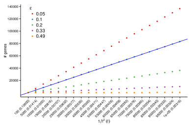
Figure 1: The number of genes below which a certain level of error ($\epsilon$) is unavoidable according to the Binomial distribution. Values on the x axis show $1/f^{2}$ where $f$ is the branch length in coalescent units ($f$ is shown parenthetically). The y axis shows the largest value of $m$ where the CDF of a binomial with parameter $1-{2}/{3}e^{-f}$ evaluated at ${m/}{3}$ is above the error level $\epsilon$. A line is fitted to points for each $\epsilon$ (shown for each line).

Before proving the lower bounds, we first present a simple numerical experiment. Suppose we want to find the $m$ below which the error probability is at least $\epsilon$ for any $\epsilon\in[0,0.5)$. We know that $P(F)$ is a lower bound on $P(E)$, and that it has the following closed form expression

$$P(F)=\sum_{i=0}^{\lfloor m/3\rfloor}{m\choose i}p^{i}(1-p)^{m-i},$$ (3)

which is simply the Cumulative Distribution Function (CDF) of a binomial calculated at $\lfloor m/3\rfloor$, where $p=1-\frac{2}{3}e^{-f}$. For given $f$ and $\epsilon$, we can compute the value of $P(F)$ for various choices of $m$. In Figure 1, we show the largest $m$ for which the computed $P(F)$ is larger than $\epsilon$. As $f^{-2}$ increases, the required number of binomial trials grows almost linearly with $f^{-2}$, with a slope that increases with decreasing $\epsilon$, as expected. This experiment suggests that for $m=\mathcal{O}(f^{-2})$, the reconstruction error for one quartet can be made arbitrarily close to $1/2$. Our next result formalizes this intuition.

Theorem 2.2.

For a species tree with $n=4$ leaves, let $f$ be the length of the single internal branch in the unrooted species tree. Then, for any $\epsilon\in[0,0.5)$, there exists an $f_{0}>0$ and a constant $d_{\epsilon}$, such that for all $m\leq d_{\epsilon}/f^{2}$ with $f\leq f_{0}$, the probability that ASTRAL* outputs the wrong quartet is at least $\epsilon$.

This theorem shows that with only four species and $m=\mathcal{O}(f^{-2})$ genes, the probability of error for ASTRAL* can be made arbitrarily close to 1/2. Thus, the lower bound and the upper bound asymptotically match as $f$ decreases.

The proof, shown in Appendix A.3, essentially uses the Berry-Esséen theorem to first approximate the binomial with a Gaussian distribution and then shows that for sufficiently small $f$, when the number of observations is below $\mathcal{O}(f^{-2})$, the Gaussian has a sufficiently large probability of deviating from its mean enough to become below 1/3.

2.2.2 Species trees of arbitrary size ($n>4$)

If all quartets in a gene tree were generated independently, extending Theorem  2.2 to more species would be trivial. However quartets have a complicated dependence structure. To establish a complement to our upper bound, it suffices to show that there exists a tree where $m=\mathcal{O}(f^{-2}\log n)$ gene trees would result in a high probability of error. We start with a simpler claim that establishes the lower bound with respect to $f$—but not $n$.

Claim 2.1.

For any $n$ and $\epsilon\in[0,0.5)$, there exists a species tree with $n$ leaves and shortest branch length $f$ such that when ASTRAL* is used with $m\leq d^{\prime}_{\epsilon}/f^{2}$ gene trees, for some constant $d^{\prime}_{\epsilon}$, the probability that ASTRAL* reconstructs the wrong tree is at least $\epsilon$.

The proof, detailed in Appendix A.4, simply uses trees of the form $(((u,v),w),\mathcal{X})$, where $\mathcal{X}$ is an arbitrary tree with $(n-3)$ leaves (represented by the set $X=[n-3]$) that is connected to the root with a very long branch. By making this branch sufficiently long, we ensure that with high probability all quartets with leaves $\{x,u,v,w\}$ for $x\in X$ have the same frequencies in the gene trees; this observation enables us to reduce the problem to the case of $n=4$ and make use of Theorem  2.2.

By construction, our result in Claim 2.1 does not depend on $n$. To match the lower bound, we strengthen this result to an upper bound that depends on both $f$ and $n$.

Theorem 2.3.

For any $\rho\in(0,1)$ and $a\in(0,1)$, there exist constants $f_{0}$ and $n_{0}$ such that the following holds. For all $n\geq n_{0}$ and $f\leq f_{0}$, there exists a species tree with $n$ leaves and shortest branch length $f$ such that when ASTRAL* is used with $m\leq\frac{a}{5}\frac{\log n}{f^{2}}$ gene trees, the event $E$ that ASTRAL* reconstructs the wrong tree has probability

$$P(E)\geq 1-\rho.$$ (4)

Remark.

The above result tells us that, for all $n$ large enough, there exists a species tree such that when ASTRAL* is used with $m\leq\frac{a\log n}{5f^{2}}$ gene trees, the probability of error is bounded away from zero. This lower bound can be made arbitrarily close to 1 (as $n$ goes to infinity).

The proof (Appendix A.5) uses ideas similar to Claim 2.1; instead of using one construct of the form $((u,v),w)$ matched with $x\in\mathcal{X}$ (as we did for Claim 2.1), we use $n/3$ such constructs (each called a triplet). We show that each triplet, when matched with one more leaf to build a quartet, has a probability of error of at least $\Omega(\frac{1}{n^{a}})$. We then argue that when branches above all triplets are long enough, error events for individual triplets can be made independent conditioned on each triplet coalescing in its root branch. Finally, the conditional independence of $\Omega(n)$ error events and the $\Omega(\frac{1}{n^{a}})$ lower bounds are used to derive the bound.

2.3 Summary of results

We showed that the upper bound on the required number of genes for ASTRAL* to reconstruct the correct species tree with high probability grows as $f^{-2}\log n$. We further proved that there exist parts of the species tree space where this upper bound is tight in the sense that the probability of error can be bounded strictly away from zero when the number of input gene trees is of order $f^{-2}\log n$. Thus, ASTRAL* requires $\Omega(f^{-2}\log n)$ gene trees to universally guarantee correct species tree reconstruction with high probability.

3 Simulations

We now study the performance of ASTRAL-II and the NJst approach [30] in simulations. We seek to find the number of genes required by each method to recover the true unrooted species tree with high probability. We test ASTRAL-II, version 4.10.10 [36] and NJst as implemented in ASTRID [52].

3.1 Simulation procedures

Testing sample complexity in simulations requires care. We seek the minimum number of genes with which methods stay under a specific level of error for specific model trees.

3.1.1 Model species trees

We study three different tree forms, shown in Figure 2(a), all with exactly $n=8$ species and varying branch lengths (in coalescent units). The three forms we test are a fully unbalanced tree where all internal branches have length $f$, a fully balanced tree where all internal unrooted branches have length $f$, and a balanced tree where the two branches incident on the root have length 30 (i.e., very long) and the remaining branches have length $f$. We refer to these trees as caterpillar, balanced, and double-quartet, respectively. We use nine values for $f$ in the range $[0.005,0.1]$, spaced so that $1/f^{2}$ is divided into equal chunks.

Table 2: Anomaly zone Conditions. For each each species tree topology and the smallest and the largest value of $f$, we show the rank of the species tree topology among the 10395 unrooted gene trees, its probability, and the probability of the most likely gene tree other than the species tree.

Tree	$f$	ST rank	$p(S)\times 10^{4}$	$p(g^{t})\times 10^{4}$
Caterpillar	0.1	50	$8.708$	$13.671$
Caterpillar	0.005	6028	$0.698$	$2.420$
Balanced	0.1	1	$28.096$	$23.170$
Balanced	0.005	1	$2.5694$	$2.5690$
Double-quartet	0.1	1	$247.843$	$143.215$
Double-quartet	0.005	1	$128.457$	$124.679$

The unrooted anomaly zone requires at least two consecutive short branches (often defined as below 0.1) [14]. Based on calculations carried by the hybrid-coal software [56],the caterpillar tree is in the anomaly zone, but the balanced tree and the double quartet trees are not (Table 2). More importantly, most of the branch lengths we have used are extremely short and go beyond what one might expect in most real biological datasets. With $f=0.1$, assuming a diploid population size of 100,000, the branch would represent 20,000 generations (or roughly 100,000 years assuming a generation time of 5 years). In our simulations with $f=0.1$, the percent of quartets that agree with each branch (computed by ASTRAL-II [47]) is never more than 46%. Thus, $f=0.1$ represents short branches, but is within ranges observed in biological datasets. On the other end, using the same assumptions, $f=0.005$ corresponds to a branch of only 1,000 generations, which is perhaps unrealistically short, and close to the range where biologists would consider a hard polytomy. In our simulations, all branches except the one long internal branch in the double-quartet tree (note that in the unrooted version, the double-quartet tree has only one long branch) result in high levels of discordance. For $f<0.1$, the quartet support for species tree branches is very close to 1/3 (i.e., random) and is never more than 36%.

Thus, we emphasize that our choice of branch lengths is motivated by a desire to explore the ability to reconstruct the species tree under extreme conditions and establishing trends in data requirement; we refer the reader to earlier publications for simulations seeking to emulate realistic conditions [35, 36].

For each species tree, gene trees are generated according to the MSC model using the Dendropy package [49].

3.1.2 Number of replicates and $\epsilon$

We seek to find the smallest number of gene trees, $m$, so that the probability of incorrect tree reconstruction by each method is no more than $\epsilon=0.1$. Computing the exact $\epsilon$ for a given $m$ in simulations requires an infinite number of replicates. In our simulations, for each species tree, we simulate 401 replicate datasets, with varying number of genes. To approximately achieve $\epsilon=0.1$, we search for the smallest $m$ such that in no more than 40 replicates each method outputs an incorrect species tree. Using normal approximation for binomial, observing 40 error events out of 401 replicates gives us a 90% confidence interval of $(0.075,0.124)$ for $\epsilon$. Getting 90% confidence intervals of $0.1\pm 0.01$ would require close to 2,500 replicates, which is computationally infeasible given the number of genes required per replicate.

3.1.3 Binary search for $m$

Finding $m$ requires running ASTRAL-II and NJst with increasing numbers of genes until reaching error levels below the specified threshold. Since our choices of $f$ require tens of thousands of gene trees, this approach would become computationally impractical. Instead, we use a binary search to find a tight window around the true value of $m$. The binary search starts with an initial range for $m$, picked as a guess by dividing results presented in Theorem 2.1 by 20. We set $m$ to the midpoint of the range and estimate $\epsilon$ by counting the number of replicates where each method outputs an incorrect tree. Based on the estimated $\epsilon$, we then decide to narrow down the range to the portion above or below the midpoint, and we repeat the process. We stop when the range becomes narrow enough (1/20 of our initial guess). We depict final ranges and fit lines to their midpoints. Additionally, we check that upper and lower halves have been each chosen at least in one iteration of the binary search. This is to ensure that the true $m$ is within our initial range, and in occasions where this was not true, we expanded the initial range.

3.2 Results

Results of our simulations are shown in Figure 2. As expected, decreasing $f$ results in increased data requirements for both methods. The average number of genes required by ASTRAL-II ranges from 206, 255, or 297 genes, respectively for the balanced, caterpillar, or double-quartet trees with $f=0.1$, to $48948$, $59528$, and $93750$ genes with $f=0.005$. Matching our theoretical results, the number of genes required by ASTRAL-II increased proportionally to $1/f^{2}$. Similarly, NJst seems to have data requirements that scale with $1/f^{2}$ under these model conditions. Interestingly, the tree shape had a substantial and somewhat surprising impact on the exact number of required genes.

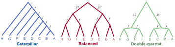
(a)

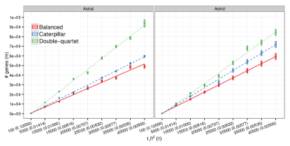
(b)

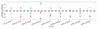
(c)

Figure 2: Data requirement of ASTRAL-II and NJst (implemented in ASTRID) in simulations with $\epsilon=0.1$. For each of the three different species tree shapes (panel a) and values of $f$, the length of the shortest branch, 401 replicate datasets are simulated using the MSC model, each with up to $10^{5}$ gene trees. (b) A binary search is used to find an approximate range for the smallest number of genes with which ASTRAL-II (left) or NJst (right) recover the correct tree in at least 90% of the 401 replicates. Boxes show these ranges and the horizontal lines show the midpoint of each range. A line is fitted to midpoints for each tree shape. (c) The ratio of the number of genes required by ASTRAL-II to the number required by NJst; below 1.0 indicates ASTRAL-II is better.

With both methods, the caterpillar tree required slightly more genes than the balanced tree, a result that we don’t find surprising as we will discuss. However, counter-intuitively, when the first two branches in the balanced tree were made extremely large (i.e., the double-quartet tree), the data requirement for both methods went up, and the increase was more dramatic for ASTRAL-II. For example, for $f=0.00816$, the balanced tree requires 21,096 gene trees, while the double-quartet requires 36,115, an increase of about 70%. Comparing the data requirement of ASTRAL-II and NJst reveals that ASTRAL-II typically required between 10 to 20% fewer genes for the caterpillar and balanced trees, while NJst required fewer genes for the double quartet tree.

The results show that the data requirement of ASTRAL-II and its relative performance depend on the tree shape as well as on the exact pattern of branch lengths. We provide possible explanations for the surprising results in the Discussion section. The results also suggest that the sample complexity of NJst might be also quadratic with respect to $1/f$.

4 Discussion

The results we presented heavily rely on properties of the MSC model, which assumes that genes evolve in an i.i.d. fashion. This assumption, which is perhaps biologically unrealistic, enables us to treat true gene trees as draws from a multinomial distribution over the discrete space of all tree topologies, and hence provide a nice mathematical framework for studying sample complexity. The main remaining difficulty in analyzing the MSC process is the fact the tree space is combinatorial and hard to enumerate. Luckily, using quartets provides a way to address this challenge because there are only three possibilities for an unrooted tree topology, and moreover, the anomaly zone does not exist. The analysis of ASTRAL* sample complexity for quartets mostly reduces to analyzing the concentration of a multinomial distribution with three probabilities $(1-\frac{2}{3}e^{-f},\frac{1}{3}e^{-f},\frac{1}{3}e^{-f})$; thus, we can use the well-established Hoeffding concentration inequality and the standard union bound technique to deal with dependencies for upper bounds. In the case of lower-bounds, even though the quartet case reduces to analyzing the CDF of binomials (Fig. 1), the binomial CDF function has a complex dependence on the parameter $m$, which motivates us to use the Berry-Esséen theorem (which essentially is a stronger version of the Central Limit Theorem) and also more strong bounds specific to binomials. Extending lower bound results from quartets to arbitrary $n$ is not quite as easy as the upper bounds because simple methods like union bounds are not available. Instead, we exploit the properties of the MSC model to design species trees with sufficiently long branches, and this makes the quartets independent conditioned on events of an arbitrarily high probability. To summarize, the key to obtaining our results is to reduce large $n$ cases to $n=4$, and to then turn the problem into the analysis of binomial distributions defined by MSC model.

4.1 Gene tree error

Throughout the paper, we assumed a random sample of true gene trees generated by the MSC model is given. However, in practice, the gene trees are reconstructed from sequence data, and hence might contain errors. Moreover, processes other than ILS may contribute to gene tree discordance. These violations of assumptions have the potential to invalidate our results. One may suspect that when violations are not severe, many of our conclusions may remain intact. We can address this conjecture using a simplistic error model.

Assume that each gene tree quartet can be incorrectly estimated with probability not exceeding some constant $e_{0}$, and also assume these events are independent across different quartets. In the event of an error, each of the two alternative topologies is assumed to be equally likely (i.e., has $1/2$ conditional probability). This model is not a realistic model of gene tree reconstruction error for a variety of reasons. Quartets and their error events are not independent. Moreover, the assumption of having unbiased error is very strong, and does not necessarily follow from properties of tree reconstruction under any of the realistic models of sequence evolution. Nevertheless, the following result provides insights about robustness of our results.

Let us denote by $Q_{i}$ the probability distribution according to the MSC model for the quartet $i$, i.e., $Q_{i}=\{p_{i},r_{i},r_{i}\}$ is the probability distribution on the set of the three possible topologies of the $i^{th}$ quartet. Then under the above error assumption, the observed quartets will have a probability distribution $Q_{i}^{\prime}=\{p_{i}^{{}^{\prime}},r_{i}^{{}^{\prime}},r_{i}^{{}^{\prime}}\}$, with $p_{i}^{{}^{\prime}}\geq p_{i}(1-e_{0})+r_{i}e_{0}$, and $r_{i}^{{}^{\prime}}\leq r_{i}(1-e_{0}/2)+p_{i}e_{0}/2$. As long as $p_{i}^{{}^{\prime}}>r_{i}^{{}^{\prime}}$, the upper bound for $m$ will have the same form as in Eq.5, but with larger constants. A sufficient condition for this to happen is $p_{i}(1-e_{0})+r_{i}e_{0}>1/3$ or $e_{0}<2/3$. Thus, with this particular error model, up to 66% of gene trees can be incorrectly estimated and our sufficient conditions for correct reconstruction using ASTRAL* will not asymptotically change, indicating some level of robustness.

A rigorous analysis of the data requirement in the presence of gene tree error requires considering gene tree inference requirements. Since a sufficient condition for accurate gene tree inference is having genes with length that scales as $f^{-2}$ [21], one may expect that $m$ and the length of each gene both growing like $f^{-2}$ will be sufficient to bound error. This will result in total data requirement that scales with $f^{-4}$. The METAL [13] method that estimates species tree directly from sequence data has $f^{-2}$ overall data requirement (using short constant-length genes), but it has remained theoretical and its performance on data remains untested.

4.2 ASTRAL-I and ASTRAL-II

The constrained versions, ASTRAL-I and ASTRAL-II (see Table 1), proceed similarly to ASTRAL*, with the added constraint that they restrict the species tree to draw its bipartitions from a fixed set ($X$). ASTRAL-I sets $X$ to the input set of gene trees, and ASTRAL-II further expands the set of allowable bipartitions using various heuristics. Clearly, any sufficient condition for ASTRAL-I to recover the true species tree will also be sufficient for ASTRAL-II, but necessary conditions for ASTRAL-II need not be as restrictive as ASTRAL-I.

Analyzing the data requirement of ASTRAL-I requires answering the following question: how many genes are needed before every bipartition of the species tree has an arbitrarily high probability of appearing in at least one gene tree. To our knowledge, a recent result by Uricchio et al. is the only work on this “bipartition cover” problem [51]. Uricchio et al. give upper bounds on the required number of genes and, as our Appendix B shows, their upper bound correspond to an $m$ that increases as $\Theta(f^{-(n-3)})$. If that many genes were to be proved also necessary, we would conclude that ASTRAL-I and ASTRAL* have dramatically different data requirements. However, these analyses are very conservative and likely give only very loose upper bounds; the data requirement of the bipartition cover problem may prove to be much less. Tighter bounds for the bipartition cover problem are challenging to derive and need to be addressed in future work.

4.3 Discussion of simulation results

In simulations, we found the species tree to be consequential for the required number of genes for both methods. Understanding the exact impact of tree shape would require a more extensive study. Here we provide some conjectures.

The fact that caterpillar trees required more genes compared to balanced trees is not due to increased discordance. For example, both trees had a quartet score of 44% with $f=0.1$ or 34% with $f=0.005$ (computed based on 2000 simulated gene trees), indicating identical levels of gene tree discordance. However, differences in data requirements of ASTRAL-II may be explained by the dependency structure of quartets. We say a quartet is defined around an internal branch of a tree if the middle path of the quartet corresponds exactly to that branch. Take the “centroid” branch in each tree that divides the leaves into two sets of size four. In the caterpillar tree, there are nine quartets around the centroid branch, and all these nine quartets share at least two leaves (E and D). In the balanced tree, there are sixteen quartets around the centroid branch, and eight pairs of quartets share no leaves in common. Thus, in the caterpillar case, we have fewer quartets and quartet trees are highly dependent, providing little additional information with respect to each other. On the other hand, in the balanced tree, we have more quartets and many of them share few or no taxa and so, intuitively, may be less dependent. Note that having less dependence in the quartets around a branch can potentially help ASTRAL-II because even if the binomial associated with one of the quartets happens to give a score below $m/3$ for the species tree resolution, the other quartets can potentially make up for it. In other words, having fully independent quartets around a branch is like having more genes as input; balanced trees have more quartets and less dependence among quartets compared to caterpillar trees.

We also observed that the double-quartet tree requires many more genes than the balanced tree. This is counter-intuitive because the longer branch in the double-quartet tree reduces gene tree discordance. In our simulations, the model balanced tree had quartet scores of 44% and 34% for $f=0.1$ and $f=0.005$ while the double-quartet tree had scores of 71% and 68% (computed based on 2000 simulated gene trees). Why does the double-quartet tree require more genes despite having dramatically less discordance?

The pattern may be related to quartet dependencies. The long branch at the root of the double-quartet tree results in a high likelihood that all lineages coalesce before reaching the root. For example, take the parent of $(H,G)$; quartets around that branch include $H$, $G$, $E$ or $F$, and one of $\{A,B,C,D\}$ (Fig. 2); all quartets that include $F$ will all have the same exact frequency (same for $E$), hence providing no additional information with respect to each other. Thus, the long branch at the top is causing the eight quartets around each of the four lower branches to have very redundant information; this redundancy is unhelpful, as we discussed earlier. Thus, counter-intuitively, reduced discordance at the basal branch may also be resulting in more uncertainty about resolutions of the branches closer to the tips. The double-quartet tree that looks easier in terms of gene tree discordance turns out to be more difficult for ASTRAL-II to resolve correctly. Our results do not imply that the long branch itself is hard to recover. It simply indicates that it may complicate the recovery of short branches. This pattern, if observed more broadly, would incidentally resemble the long branch attraction problem in sequence-based analyses. We note that the conditions where ASTRAL-II had surprisingly high data requirements resemble the types of trees that we invoked to prove the lower bounds for arbitrary $n$.

Finally, our simulations start to shed light on differences between conditions where ASTRAL-II and NJst can each be expected to work better. In model conditions where all branches where short, ASTRAL-II outperformed NJst, especially with caterpillar trees. Both methods were sensitive to the presence of long branches, but ASTRAL-II more so. More broadly, our research indicates that a thorough examination of tree shapes for which ASTRAL and NJst perform well is required. Finally, the simulation results lead to the conjecture that NJst also requires $\mathcal{O}(f^{-2})$ gene trees; we hope future work will prove or disprove this conjecture.

4.4 Practical implications

Asymptotic results are not meant to provide practitioners with means to predict how many gene trees are needed. Two issues hamper such a goal. On the one hand, some of the parameters of the species tree (e.g., $f$) are not known in advance. On the other hand, the lower and upper bound values match only asymptotically and in practice, the effect of the unknown constants is important. Practitioners trying to decide the number of required genes in advance may be only marginally helped by our results. For example, given a large number of loci sampled from a few species (e.g., those with full genomes sequenced), they can empirically estimate the number of required genes (e.g., judging accuracy by examining local posterior probabilities generated by ASTRAL [47]). Then, to predict the number of required genes if they were to sample more species, they could extrapolate using our results; this would still need guessing the reduction in $f$ due to increased sampling and such estimates will have to be taken as ballpark guesses.

Sample complexity results are useful to judge the effectiveness of methods. The best possible sample complexity for the problem of inferring species trees from gene tree topologies is not known. If future work proves $\mathcal{O}(f^{-2})$ to be the best possible, our results will give practitioners reasons to have confidence in the efficiency of ASTRAL. On the other hand, if some other tool is ever proved to have a better sample complexity, such asymptotic results should give practitioners some indication that alternative algorithms may be preferable. In either case, asymptotic results are not a replacement for careful empirical and simulation studies and should be used as a complementary source of information when judging methods.

Appendix A Proofs

A.1 Notation and definitions

We denote the number of species by $n$ and the number of gene trees by $m$. Let $k={n\choose 4}$ denote the total number of quadruples of leaves, also known as quartets, in the species tree. We use $[k]$ to represent the set $\{1,2\ldots,k\}$.

For each quartet $i\in[k]$, let $q_{i}$ represent the unrooted tree topology induced by the species tree for quartet $i$. There are three possible unrooted tree topologies that can be induced by gene trees and we represent these three configurations by $q_{i1},q_{i2}$, and $q_{i3}$. We choose to use $q_{i1}$ to denote the configuration of the species tree, i.e., $q_{i1}=q_{i}$. Also let $n_{ij}$, for $j=1,2,3$, represent the number of gene trees that induce the $q_{ij}$ topology. By definition, $\sum_{j=1}^{3}n_{ij}=m$ for all $i\in[k]$.

Under the MSC model, for each $q_{i}$, the probability that a gene tree has configuration $q_{i1}$ is $p_{i}=1-\frac{2}{3}e^{-d_{i}}$ where $d_{i}$ is the length of the middle path in the quartet topology of the species tree measured in coalescent units [4]. The other two configurations have equal probability $r_{i}=(1-p_{i})/2$. Let us denote by $\delta_{i}$ the quantity $p_{i}-1/3$ and let $\delta$ be the minimum over all $\delta_{i}$s. All quartets defined around the shortest branch in the species tree have $\delta_{i}=\delta$ and we use $f$ to denote the length of this shortest species tree branch.

ASTRAL* returns the species tree that maximizes the score $s(T)=\sum_{i=1}^{k}n_{i,t_{i}(T)}$ where $t_{i}(T)$ gives the index of the topology for quartet $i$ found in tree $T$. Hence observe that the score of the true species tree is $\sum_{i=1}^{k}n_{i1}$.

A.2 Proof of Theorem 2.1

Theorem 2.1. Consider a model species tree with minimum branch length $f<\log(\sqrt{2})$. Then, for any $\epsilon>0$, ASTRAL* returns the true species tree with probability at least $1-\epsilon$ if the number of input error-free gene trees satisfies

$$m>\frac{9}{2}\log\bigg{(}\frac{4{n\choose 4}}{\epsilon}\bigg{)}\frac{1}{(1-e^{-f})^{2}}.$$ (5)

To prove this result, we require an upper bound on the probability of error in terms of $m$, $n$ and $f$. For that, we observe that a sufficient condition for ASTRAL* to return the correct species tree is that for all the quartets $i\in[k]$, the true topology is observed in a majority of the $m$ gene trees, i.e., $n_{i1}>\max\{n_{i2},n_{i3}\}$. Thus, for ASTRAL* to make an error, at least one quartet must have an alternate topology in a majority of the gene trees. We upper bound the probability of this event for one quartet by using Hoeffding’s inequality, and then take a union bound over all quartets to bound the overall probability of error.

Let $w<\delta/2$. We use $A_{i}$ to refer to the event $n_{i1}/m\in(p_{i}-w,p_{i}+w)$, and use $B_{i}$ and $C_{i}$ to refer to events $n_{i2}/m\in(r_{i}-w,r_{i}+w)$ and $n_{i3}/m\in(r_{i}-w,r_{i}+w)$, respectively.

Lemma A.1.

For any $w<\delta/2$, ASTRAL* is guaranteed to return the true species tree if the event $D_{i}=A_{i}\cap(B_{i}\cup C_{i})$ occurs for all $i\in[k]$.

Proof.

Recall the definition of the score $s(T)$ and observe that ASTRAL* returns the true species tree when the following condition holds:

$$n_{i1}>\max\{n_{i2},n_{i3}\},\qquad\forall i\in[k].$$

We claim that, for all values of $w$ smaller than $\delta/2$, we can ensure that $n_{i1}$ is the largest among $n_{ij}$, when the event $D_{i}$ occurs. Indeed, let $D_{i}$ hold and assume w.l.o.g. that $B_{i}$ occurs. In the worst case, $n_{i1}=(p_{i}-w)m$ and $n_{i2}=(r_{i}-w)m$, which results in $n_{i3}=(r_{i}+2w)m$ because the sum of all three $n_{ij}$s is $m$. In this case, we need $r_{i}+2w=(1-p_{i})/2+2w<p_{i}-w$, or after multiplying by $2$ and rearranging $3p_{i}-1>6w$. This is true for all $w<\frac{1}{2}\delta_{i}=\frac{1}{2}(1/3-p_{i})$. ∎

Lemma A.2.

Suppose the input to ASTRAL* is $m$ true gene trees generated under the MSC model. For every $\epsilon>0$, ASTRAL* reconstructs the correct species tree with probability at least $1-\epsilon$ if

$$m>2\log\bigg{(}\frac{4{n\choose 4}}{\epsilon}\bigg{)}\frac{1}{\delta^{2}}.$$ (6)

Proof.

If $E$ denotes the event that ASTRAL* returns the wrong species tree, then by Lemma A.1 we have by a union bound

$$P(E) \leq P\big{(}\cup_{i=1}^{k}D_{i}^{c}\big{)}$$ (7)

$$=P(\cup_{i=1}^{k}A_{i}^{c}\cup(B_{i}^{c}\cap C_{i}^{c}))$$ (8)

$$\leq P\big{(}\cup_{i=1}^{k}(A_{i}^{c}\cup B_{i}^{c})\big{)}$$ (9)

$$\leq\sum_{i=1}^{k}\left[P(A_{i}^{c})+P(B_{i}^{c})\right]$$ (10)

Thus we need a bound on $P(A_{i}^{c})$ and $P(B_{i}^{c})$. Let us define a random variable $X_{ig}$, for $i\in[k]$ and $g\in[m]$, which takes the value 1 if the configuration of the $i^{th}$ quartet in the $g^{th}$ gene tree is the same as $q_{i}$; and is zero otherwise. Then $(X_{ig})_{g=1}^{m}$ is a sequence of independent Bernoulli random variables with parameter $p_{i}$ and $n_{i1}=\sum_{g=1}^{m}X_{ig}$. The event $A_{i}^{c}=\{n_{i1}\notin(m(p_{i}-w),m(p_{i}+w))\}$ with $w<\frac{\delta}{2}$ becomes increasingly unlikely as $m$ grows and its probability can be bounded using Hoeffding’s inequality (see e.g.[33]) to get

$$P(A_{i}^{c})\leq 2e^{-2mw^{2}}.$$

The same bound holds for $P(B_{i}^{c})$. Plugging this into (7), we get

$$P(E)\leq{n\choose 4}4e^{-2mw^{2}}.$$ (11)

To make the Right Hand Side (RHS) smaller than $\epsilon$, we take

$$m\geq\frac{1}{2w^{2}}\log\bigg{(}\frac{4{n\choose 4}}{\epsilon}\bigg{)}.$$ (12)

The result follows from the fact that we can choose any $w<\delta/2$.∎

Proof of Theorem 2.1.

Lemma A.2 gives us the gene tree requirement in terms of the parameter $\delta$. The result in Theorem 2.1 immediately follows by replacing $\delta$ with $\frac{2(1-e^{-f})}{3}$. In the limit of small $f$, we note further that $\frac{(1-e^{-f})^{2}}{f^{2}}$ increases to 1. This gives the $\mathcal{O}(f^{-2})$ dependence of the bound on $m$ as mentioned in the Remark after the statement of the theorem.∎

A.3 Proof of Theorem 2.2

Theorem 2.2. For a species tree with $n=4$ leaves, let $f$ be the length of the single internal branch in the unrooted species tree. Then, for any $\epsilon\in[0,0.5)$, there exists an $f_{0}>0$ and a constant $d_{\epsilon}$, such that for all $m\leq d_{\epsilon}/f^{2}$ with $f\leq f_{0}$, the probability that ASTRAL* outputs the wrong quartet is at least $\epsilon$.

Proof.

We divide the proof into two cases. First we show that the result holds for $m\leq c_{\epsilon}/f$, for some constant $c_{\epsilon}$. That follows from the fact that, in that case, a non-trivial fraction of genes coalesce only in the ancestral root population. We then show separately that the result also holds for $c_{\epsilon}/f<m<d_{\epsilon}/f^{2}$, for some choice of $d_{\epsilon}$. There, we use the Berry-Esséen theorem to control the probability that a majority of the genes return the wrong topology.

Case 1 ($m\leq c_{\epsilon}/f$)

Let $G$ be the event that, in all gene trees, all the lineages reach the root population without any prior coalescence. Depending on the rooting, the quartet species tree can either have the symmetric topology or the asymmetric topology. In both cases we have

$$P(G)=(e^{-f})^{m}=e^{-mf}.$$ (13)

(Recall that $f$ represents the internal branch length in the unrooted tree. Thus it equals the length of the single internal branch in the asymmetric case and it equals the sum of the two internal branch lengths in the symmetric case.)

Under $G$, for every gene tree, all three topologies are equally likely. So $n_{11},n_{12}$ and $n_{13}$ have the same distribution. (There is only one quartet in this case.) Since ASTRAL* selects the output tree randomly in case of a tie, by symmetry we can conclude that $P(E|G)=2/3$ and hence, by (13),

$$P(E)\geq P(E|G)P(G)\geq\frac{2}{3}e^{-c_{\epsilon}}.$$

For all $\epsilon\in[0,0.5)$, the choice $c_{\epsilon}=\log(\frac{2}{3\epsilon})$ ensures finally that $P(E)\geq\epsilon$.

Case 2 ($c_{\epsilon}/f<m<d_{\epsilon}/f^{2}$)

Recall that, when $n=4$, we let $F$ be the event that $\{n_{11}\leq m/3\}$. We write

$$P(F)=P(n_{11}\leq m/3)=P(Y\leq y)$$

where $Y=\frac{n_{11}-pm}{\sqrt{p(1-p)m}}$ and $y=\frac{-m(p-1/3)}{\sqrt{p(1-p)m}}$. Then, by the Berry-Esséen theorem (as stated e.g. in [18]), we have

$$\bigg{|}P(Y\leq y)-\Phi(y)\bigg{|} \leq\frac{cp(1-p)[p^{2}+(1-p)^{2}]}{[p(1-p)]^{3/2}m^{1/2}}$$

$$\leq\frac{cp}{[p(1-p)]^{3/2}m^{1/2}},$$

where $\Phi(\cdot)$ denotes the normal CDF and $c$ is a universal constant (which can be taken to be $3$). Thus

$$P(F)=P(Y\leq y)\geq\Phi(y)-\frac{cp}{[p(1-p)]^{3/2}m^{1/2}}.$$ (14)

It remains to show that the RHS above is bounded away from $0$ when $f$ is small. We estimate the two terms separately. We know that as $f\to 0$, $p\to 1/3$ and $p(1-p)\to 2/9$, and $p(1-p)$ is monotonic for $0<p<1/2$. Thus, there exists an $f_{1}$ such that $p\leq 10/27$ and $p(1-p)\geq 1/9$ whenever $f\leq f_{1}$. So, for all $f\leq f_{1}$,

$$y=\frac{m^{1/2}(p-1/3)}{(p(1-p))^{1/2}} \leq 3m^{1/2}(p-1/3),$$

and

$$\frac{cp}{(p(1-p))^{3/2}m^{1/2}} \leq\frac{10c}{m^{1/2}}.$$

Thus we get the following relation

$$P(F)\geq\Phi\big{(}-3m^{1/2}(p-1/3)\big{)}-\frac{10c}{m^{1/2}}.$$ (15)

Let us first consider the second term on the RHS. For $m>c_{\epsilon}/f$,

$$\frac{10c}{m^{1/2}}<\frac{10cf^{1/2}}{c_{\epsilon}^{1/2}}$$

Let $\bar{f}_{2}$ be such that $\frac{10c\sqrt{\bar{f}_{2}}}{\sqrt{c_{\epsilon}}}=\frac{\gamma}{2}$, for $\gamma=1/2-\epsilon$. For all $f\leq f_{2}=\text{min}\{\bar{f}_{2},f_{1}\}$ and $m>c_{\epsilon}/f$, we have $10c/\sqrt{m}<\gamma/2$.

As for the first term on the RHS of (15), it is decreasing in $m$ for a fixed $f$. Thus for any $f\leq f_{2}$, if we find a value of $m$ as a function of $f$, say $m_{0}(f)$, which is larger than $c_{\epsilon}/f$ and for which this first term is no smaller than $1/2-\gamma/2$, then the required result also holds for all $m\in(c_{\epsilon}/f,m_{0}(f)]$.

Let us set $m_{0}(f)=d_{\epsilon}/f^{2}$, where $d_{\epsilon}$ will be determined below. Then we have

$$P(F) \geq\Phi\left(-3\sqrt{d_{\epsilon}}\left(\frac{2}{3}\left(\frac{1-e^{-f}}{f}\right)\right)\right)-\frac{\gamma}{2}$$ (16)

$$=\Phi\left(-2\sqrt{d_{\epsilon}}\right)-\frac{\gamma}{2},$$ (17)

where we used that for $f>0$, $\frac{1-e^{-f}}{f}\leq 1$. Now, if we set

$$d_{\epsilon}=\bigg{(}\frac{\Phi^{-1}\left(1/2-\gamma/2\right)}{2}\bigg{)}^{2}$$ (18)

we get that, for all $f\leq f_{2}$ and $m\in(c_{\epsilon}/f,d_{\epsilon}/f^{2}]$, $P(E)\geq 1/2-\gamma=\epsilon$. Finally, we define $f_{0}=\text{min}\{f_{2},d_{\epsilon}/c_{\epsilon}\}$ to ensure that the above interval is non-empty. ∎

A.4 Proof of Claim 2.1

Claim 2.1. For any $n$ and $\epsilon\in[0,0.5)$, there exists a species tree with $n$ leaves and shortest branch length $f$ such that when ASTRAL* is used with $m\leq d^{\prime}_{\epsilon}/f^{2}$ gene trees, for some constant $d^{\prime}_{\epsilon}$, the probability that ASTRAL* reconstructs the wrong tree is at least $\epsilon$.

Proof.

The idea is to reduce the proof to the case of Theorem 2.2 with an appropriate choice of species tree. We consider a species tree with the topology $(((a,b),c),\mathcal{X})$, where $\mathcal{X}$ is an arbitrary tree with $(n-3)$ leaves, which we denote by $X=[n-3]$ for convenience. We denote the edge above $(a,b)$ by $e$ and set its length to $f$. We also set the length of the the branch above $\mathcal{X}$ to $g$, a large value which we will specify later.

For $x\in X$, let $n_{x1},n_{x2},n_{x3}$ be the frequencies of the quartet trees congruent with the unrooted topology of $(((a,b),c),x)$, $(((a,c),b),x)$, and $(((a,x),b),c)$ respectively. When $n_{x1}<m/3$ for all $x\in X$, ASTRAL* cannot output the true tree. To see this, note that, under that condition, $\sum_{x\in X}n_{x1}<m(n-3)/3$; thus, $\max\{\sum_{x\in X}n_{x2},\sum_{x\in X}n_{x3}\}>m(n-3)/3$. W.l.o.g. assume that $\sum_{x\in X}n_{x2}>m(n-3)/3$. Then a tree that includes the branch $e$ cannot have the maximal score because the unrooted topology of $(((a,c),b),\mathcal{X})$ will have a higher score. Indeed, observe that all quartets not of the form $\{a,b,c,x\}$ for some $x\in X$ contribute equally to the unrooted topologies of $(((a,b),c),\mathcal{X})$ and $(((a,c),b),\mathcal{X})$.

Let $H_{i}$ denote the event that, in gene $i$, all lineages from $X$ coalesce before reaching the root branch (i.e., within or below the long branch with length $g$) and let $H=\cap_{i=1}^{m}H_{i}$. Under the event $H$, $n_{xj}=n_{yj}$ for all $x,y\in X$ and all $j\in\{1,2,3\}$; hence $P(\cap_{x\in X}n_{xj}<m/3|H)=P(n_{1j}<m/3|H)$. Thus, $\{n_{1j}<m/3\}$ is sufficient to produce the wrong topology. We now bound the probability of that event.

Let us define

$$\epsilon_{1}=\frac{1}{4}+\frac{1}{2}\epsilon,=\epsilon+\frac{1}{2}\left(\frac{1}{2}-\epsilon\right)>\epsilon$$

and

$$\eta=1-\epsilon/\epsilon_{1}.$$

From Theorem 2.2, we know that there exists an $f_{0}$ such that, for all $f\leq f_{0}$, if $m\leq d_{\epsilon_{1}}/f^{2}$, then $P(n_{1j}<m/3|H)\geq\epsilon_{1}$. Let

$$m_{0}=m_{0}(f)=d_{\epsilon_{1}}/f^{2},$$

as defined in the proof of Theorem 2.2. If $E$ denotes the event that ASTRAL* produces the wrong output, then we have

$$P(E)\geq P(n_{1j}<m/3|H)P(H)\geq P(H)\epsilon_{1}.$$ (19)

Proving a lower bound of $1-\eta$ for $P(H)$ then implies the result, by our choice of $\eta$. For this, we choose appropriately the value of $g$. Specifically, we pick $g$ large enough to ensure that $P(H_{i})\geq 1-\eta_{1}$ for $\eta_{1}=1-(1-\eta)^{1/m_{0}}$. Due to the independence of the genes, we get that for all $m\leq m_{0}$

$$P(H)\geq(1-\eta_{1})^{m}\geq(1-\eta_{1})^{m_{0}}=1-\eta.$$ (20)

Combining this with (19), we get that $P(E)\geq\epsilon$. Thus, we have shown the existence of a tree with $n$ leaves for which ASTRAL* is wrong with probability at least $\epsilon\in[0,0.5)$ if the number of input gene trees is less than or equal to $d^{\prime}_{\epsilon}/f^{2}$, where $d^{\prime}_{\epsilon}=d_{\epsilon+1/2(1/2-\epsilon)}$.∎

A.5 Proof of Theorem 2.3

Theorem 2.3. For any $\rho\in(0,1)$ and $a\in(0,1)$, there exist constants $f_{0}$ and $n_{0}$ such that the following holds. For all $n\geq n_{0}$ and $f\leq f_{0}$, there exists a species tree with $n$ leaves and shortest branch length $f$ such that when ASTRAL* is used with $m\leq\frac{a}{5}\frac{\log n}{f^{2}}$ gene trees, the event $E$ that ASTRAL* reconstructs the wrong tree has probability

$$P(E)\geq 1-\rho.$$ (21)

Proof.

To simplify the presentation, we assume that $n$ is divisible by three. (It is straightforward to generalize the argument.) Consider a species tree constructed as follows. Make $n/3$ rooted triplet trees all of them with an internal branch of length $f$ and arbitrarily index the triplet trees by $i\in[n/3]$. Then, pick any arbitrary tree with $n/3$ leaves labeled by $[n/3]$ and all branch lengths equal to exactly $g$. Finally, connect each leaf of this arbitrary tree with the root of the corresponding triplet tree. Let $J_{i}$ denote the event that, in all gene trees, all three lineages of the triplet $i$ coalesce in its root branch. Let $J=\cap_{i=1}^{n/3}J_{i}$. We proceed in two steps:

1. First we introduce a result analogous to Theorem 2.2 with an extra $\log n$ factor in the number of genes. This gives us a smaller probability of error of the form $n^{-a}$ for some $0<a<1$ on a single quartet.

2. Then we consider the species tree above in which there are $\Omega(n)$ chances for a quartet-based error in ASTRAL* to occur and show that at least one of these happens with sufficiently large probability.

Step 1

Let us consider one of the triplets above $i\in[n/3]$, with a topology $((u,v),w)$, as well as a leaf $x$ outside of the triplet. Let $n_{i,1}$ be the number of genes with the correct species tree topology and let $F_{i}$ denote the event that $\{n_{i,1}\leq m/3\}$. For reasons that will be made clear in Step 2, we are interested in $P(F_{i}|J_{i})$. Conditioned on $J_{i}$, let $p^{\prime}_{g}$ and $r^{\prime}_{g}=(1/2)(1-p^{\prime}_{g})$ be the probabilities of observing $((u,v),(w,x))$ and $((u,w),(v,x))$ or $((v,w),(u,x))$ respectively in the unrooted gene trees. As $g\to+\infty$, $p^{\prime}_{g}\downarrow 1-(2/3)e^{-f}$. Let $g_{0}$ be large enough (as a function of $f$) so that, for all $g\geq g_{0}$, $p^{\prime}_{g}-1/3\leq(2.1/3)(1-e^{-f})$. Assume from now on that $g\geq g_{0}$.

To deal with the extra $\log n$ factor in the number of genes, we revisit (14). This time, instead of Berry-Esséen, we use a tailored estimate on the binomial. We will need the following bounds. The Kullback-Liebler divergence between two Bernoulli random variables satisfies

$$D(a\|b) =a\log\frac{a}{b}+(1-a)\log\frac{1-a}{1-b}$$

$$\leq a\left(\frac{a}{b}-1\right)+(1-a)\left(\frac{1-a}{1-b}-1\right)$$

$$=\frac{(a-b)^{2}}{b(1-b)},$$

where we used the fact that $\log x\leq x-1$. By [7, Lemma 4.7.1], we also have

$${m\choose k}p^{k}(1-p)^{m-k}\geq\frac{\exp\left(-mD\left(k/m\middle\|p\right)\right)}{\sqrt{8m(k/m)(1-k/m)}}.$$

Using these two bounds we get

$$P(F_{i}|J_{i}) =\sum_{k=0}^{m/3}{m\choose k}(p^{\prime}_{g})^{k}(1-p^{\prime}_{g})^{m-k}$$

$$\geq\sum_{k=m/3-\sqrt{2m}}^{m/3}{m\choose k}(p^{\prime}_{g})^{k}(1-p^{\prime}_{g})^{m-k}$$

$$\geq\sum_{k=m/3-\sqrt{2m}}^{m/3}\frac{\exp\left(-mD\left(k/m\middle\|p^{\prime}_{g}\right)\right)}{\sqrt{8m(k/m)(1-k/m)}}$$

$$\geq\sum_{k=m/3-\sqrt{2m}}^{m/3}\frac{1}{\sqrt{2m}}\exp\left(-mD\left(k/m\middle\|p^{\prime}_{g}\right)\right)$$

$$\geq\sum_{k=m/3-\sqrt{2m}}^{m/3}\frac{1}{\sqrt{2m}}\exp\left(-m\frac{(p^{\prime}_{g}-k/m)^{2}}{p^{\prime}_{g}(1-p^{\prime}_{g})}\right)$$

$$\geq\exp\left(-m\frac{(p^{\prime}_{g}-1/3+\sqrt{2/m})^{2}}{p^{\prime}_{g}(1-p^{\prime}_{g})}\right),$$

where we used that $p^{\prime}_{g}>1/3$ on the last line. Above we assumed, to simplify the notation, that $\sqrt{2m}$ is an integer. Using $p^{\prime}_{g}-1/3\leq(2.1/3)(1-e^{-f})$, $1-e^{-f}\leq f$ and $m\leq m_{1}(f)=(a/5)f^{-2}\log n$, we get

$$P(F_{i}|J_{i})$$

$$\ \geq\exp\left(-\frac{(a/5)\log n}{f^{2}}\cdot\frac{\{2.1f/3+f/\sqrt{(a/10)\log n}\}^{2}}{p_{g}^{\prime}(1-p_{g}^{\prime})}\right).$$

Choose constants $f_{0}$ and $n_{0}$ depending on $a$ ensuring that $f\leq f_{0}$ and $n\geq n_{0}$ imply that $p_{g}^{\prime}(1-p_{g}^{\prime})\geq 1/9$ and that the expression in curly brackets in the previous display is less than $f\sqrt{5/9}$. Then

$$P(F_{i}|J_{i}) \geq n^{-a}.$$ (22)

Step 2

For each $i\in[n/3]$, let $E_{i}$ denote the event that all quartets containing the triplet $i$ have an alternative topology (i.e., different from the species tree) in the majority. We note that, when $J_{i}$ occurs, then $F_{i}$ implies $E_{i}$. If $E$ denotes the event that ASTRAL* outputs a wrong tree, then a sufficient condition for an error to occur is that at least one of the $E_{i}$ events occurs. Under the MSC, the events $\{F_{i}\cap J_{i}:i\in[n/3]\}$ are independent. Thus,

$$P(E) \geq 1-\prod_{i\in[n/3]}[1-P(F_{i}\cap J_{i})]$$

$$\geq 1-\prod_{i\in[n/3]}[1-n^{-a}P(J_{i})],$$ (23)

by (22). It remains to bound $P(J_{i})$.

Let $1-\rho_{2}$ be the probability that the full coalescence for triplet $i$ occurs in its root branch in one gene tree. Then $P(J_{i})=(1-\rho_{2})^{m}\geq(1-\rho_{2})^{m_{1}(f)}$ for $m\leq m_{1}(f)$. Thus, for any $\rho_{1}\in(0,1)$, we can choose $g_{1}$ large enough to ensure that $g\geq g_{1}$ implies $\rho_{2}\leq 1-(1-\rho_{1})^{1/m_{1}(f)}$ and therefore $P(J_{i})\geq 1-\rho_{1}$. Assume from now on that $g\geq\max\{g_{0},g_{1}\}$.

Going back to (23), using the fact that $(1-\frac{1}{x})^{x}\leq e^{-1}$, we have

$$P(E) \geq 1-[1-n^{-a}(1-\rho_{1})]^{n/3}$$

$$\geq 1-\exp\left(-\frac{(1-\rho_{1})n^{1-a}}{3}\right)$$

$$\geq 1-\rho,$$

for $n\geq n_{1}$, for an appropriate $n_{1}$ depending on $a$.

∎

Appendix B Bipartition cover bounds

A set of gene trees is called a bipartition cover of a species tree $S$ if the set of bipartitions included in the gene trees includes all the bipartitions of $S$. In [51], the authors show that input gene trees form a bipartition cover with probability at least $q$ if

$$m\geq M_{n,q}=\frac{\log((1-q)(n-3))}{\log(1-g_{n-2,1}(f))}=\frac{C_{n,q}}{-\log(1-g_{n-2,1}(f))},$$

where $g_{n-2,1}(f)$ is the probability that $n-2$ lineages coalesce to 1 within time $f$ and $C_{n,q}$ is implicitly defined above. When $n$ is fixed, we claim that $M_{n,q}$ is $\Theta(f^{-(n-3)})$ as $f\to 0$.

Note that $g_{n-2,1}(\cdot)$ is the CDF of a random variable $T_{n-2}=\sum_{1}^{n-3}W_{i}$ where the $W_{i}$s are independent exponential waiting times with parameters $\lambda_{i}={n-1-i\choose 2}$. Thus,

$$P(T_{n-2}\leq f)\leq\prod_{i=1}^{n-3}P(W_{i}\leq f)\leq(\prod_{i=1}^{n-3}\lambda_{i})f^{n-3}.$$ (24)

Since we have $\lim_{f\downarrow 0}\frac{1-e^{-\lambda_{i}f}}{\lambda_{i}f}=1$, for $f$ small enough we have $\frac{1-e^{-\lambda_{i}f}}{\lambda_{i}f}\geq 0.9^{1/(n-3)}$ for all $i$. So we can write

$$P(T_{n-2}\leq f) \geq\prod_{i=1}^{n-3}P\left(W_{i}\leq\frac{f}{n-3}\right)$$

$$\geq 0.9\bigg{(}\prod_{i=1}^{n-3}\lambda_{i}\bigg{)}\bigg{(}\frac{f}{n-3}\bigg{)}^{n-3}.$$

Thus for small $f$ and fixed $n$, the probability $g_{n-2,1}(f)$ scales as $f^{n-3}$.

We now note that

$$M_{n,q}=C_{n,q}\frac{1}{-\log(1-g_{n-2,1}(f))}\stackrel{{\scriptstyle(a)}}{{\leq}}\frac{C_{n,q}}{g_{n-2,1}(f)},$$ (25)

where $(a)$ follows from $\log(x)\geq 1-1/x$ for positive $x$. Also, by using $\log(x)\leq x-1$ and assuming that $f$ is small enough to ensure that the upper bound on $g_{n-2,1}$ in (24) is smaller than 0.9, we have

$$M_{n,q}\geq C_{n,q}\frac{1-g_{n-2,1}(f)}{g_{n-2,1}(f)}\geq C_{n,q}\frac{0.1}{g_{n-2,1}(f)}.$$ (26)

The bounds in (25) and (26) tell us the term $M_{n,q}$ is $\Theta(f^{-(n-3)})$, which suggests that the number of trees required by heuristic ASTRAL-I is asymptotically significantly larger than that of ASTRAL*.

Thus our theoretical analysis shows that, consistently with simulation results presented in [36], for large $n$ there should be conditions where ASTRAL-I does not work well, but ASTRAL* has high accuracy. Note that ASTRAL-II has sought to close this gap heuristically and seems to have succeeded to a large extent based on simulation results [36].

References

- [1] DupTree: a program for large-scale phylogenetic analyses using gene tree parsimony. Bioinformatics, 24(13):1540–1541, 2008.
- [2] Inferring species trees from incongruent multi-copy gene trees using the Robinson-Foulds distance. Algorithms for Molecular Biology, 8:28, 2013.
- [3] Phylotranscriptomic analysis of the origin and early diversification of land plants. Proceedings of the National Academy of Sciences, 111(45):E4859–4868, 2014.
- [4] E S Allman, James H. Degnan, and J A Rhodes. Identifying the rooted species tree from the distribution of unrooted gene trees under the coalescent. J. Math. Biol., 62:833–862, 2011.
- [5] Elizabeth Allman, James H. Degnan, and John Rhodes. Species tree inference from gene splits by Unrooted STAR methods. IEEE/ACM Transactions on Computational Biology and Bioinformatics, PP(99):1–7, 2016.
- [6] Sónia C S Andrade, Marta Novo, Gisele Y Kawauchi, Katrine Worsaae, Fredrik Pleijel, Gonzalo Giribet, and Greg W Rouse. Articulating “archiannelids”: Phylogenomics and annelid relationships, with emphasis on meiofaunal taxa. Molecular Biology and Evolution, 2015.
- [7] Robert B. Ash. Information theory. Dover Publications, Inc., New York, 1990. Corrected reprint of the 1965 original.
- [8] Eric Bapteste, Leo van Iersel, Axel Janke, Scot Kelchner, Steven Kelk, James O. McInerney, David A. Morrison, Luay Nakhleh, Mike Steel, Leen Stougie, and James Whitfield. Networks: Expanding evolutionary thinking, 2013.
- [9] Bastien Boussau, GJ J Szöllősi, and Laurent Duret. Genome-scale coestimation of species and gene trees. Genome Research, 23(2):323–330, 2013.
- [10] David Bryant, Remco Bouckaert, Joseph Felsenstein, Noah A. Rosenberg, and Arindam Roychoudhury. Inferring species trees directly from biallelic genetic markers: Bypassing gene trees in a full coalescent analysis. Molecular Biology and Evolution, 29(8):1917–1932, 2012.
- [11] Johanna Taylor Cannon, Bruno Cossermelli Vellutini, Julian Smith, Fredrik Ronquist, Ulf Jondelius, and Andreas Hejnol. Xenacoelomorpha is the sister group to Nephrozoa. Nature, 530(7588):89–93, 2016.
- [12] Julia Chifman and Laura S Kubatko. Quartet Inference from SNP Data Under the Coalescent Model. Bioinformatics, 30(23):3317–3324, 2014.
- [13] Gautam Dasarathy, Robert Nowak, and Sebastien Roch. Data requirement for phylogenetic inference from multiple loci: a new distance method. IEEE/ACM Transactions on Computational Biology and Bioinformatics (TCBB), 12(2):422–432, 2015.
- [14] James H. Degnan. Anomalous unrooted gene trees. Systematic Biology, 62:574–590, 2013.
- [15] James H. Degnan and Noah A. Rosenberg. Discordance of Species Trees with Their Most Likely Gene Trees. PLoS Genet, 2(5), 2006.
- [16] James H. Degnan and Noah A. Rosenberg. Gene tree discordance, phylogenetic inference and the multispecies coalescent. Trends in ecology & evolution, 24(6):332–340, 2009.
- [17] James H. Degnan and Laura A Salter. Gene tree distributions under the coalescent process. Evolution: International Journal of Organic Evolution, 59(1):24–37, 2005.
- [18] Rick Durrett. Probability: theory and examples. Cambridge Series in Statistical and Probabilistic Mathematics. Cambridge University Press, Cambridge, fourth edition, 2010.
- [19] Julien Y Dutheil, Gertrud Mannhaupt, Gabriel Schweizer, Christian M K Sieber, Martin Münsterkötter, Ulrich Güldener, Jan Schirawski, and Regine Kahmann. A tale of genome compartmentalization: the evolution of virulence clusters in smut fungi. Genome biology and evolution, 8(3):681–704, 2016.
- [20] Scott V Edwards, Liang Liu, and Dennis K Pearl. High-resolution species trees without concatenation. Proceedings of the National Academy of Sciences of the United States of America, 104(14):5936–5941, 2007.
- [21] Peter Erdos, Mike Steel, L Szekely, and T Warnow. A few logs suffice to build (almost) all trees: Part II. Theoretical Computer Science, 221(1-2):77–118, 1999.
- [22] Thomas C Giarla and Jacob A Esselstyn. The Challenges of Resolving a Rapid, Recent Radiation: Empirical and Simulated Phylogenomics of Philippine Shrews. Systematic biology, page syv029, 2015.
- [23] Joseph Heled and Alexei J Drummond. Bayesian inference of species trees from multilocus data. Molecular Biology and Evolution, 27(3):570–580, 2010.
- [24] Chien-Hsun Huang, Renran Sun, Yi Hu, Liping Zeng, Ning Zhang, Liming Cai, Qiang Zhang, Marcus A Koch, Ihsan Al-Shehbaz, and Patrick P Edger. Resolution of Brassicaceae phylogeny using nuclear genes uncovers nested radiations and supports convergent morphological evolution. Molecular biology and evolution, 33(2):394–412, 2016.
- [25] J F C Kingman. On the genealogy of large populations. Journal of Applied Probability, 19(1982):27–43, 1982.
- [26] Manuel Lafond and Céline Scornavacca. On the Weighted Quartet Consensus problem. 2016.
- [27] Bret R Larget, Satish K Kotha, Colin N Dewey, and Cécile Ané. BUCKy: gene tree/species tree reconciliation with Bayesian concordance analysis. Bioinformatics, 26(22):2910–2911, 2010.
- [28] Christopher E Laumer, Andreas Hejnol, and Gonzalo Giribet. Nuclear genomic signals of the ’microturbellarian’ roots of platyhelminth evolutionary innovation. eLife, 4, 2015.
- [29] Liang Liu. BEST: Bayesian estimation of species trees under the coalescent model. Bioinformatics (Oxford, England), 24(21):2542–2543, 2008.
- [30] Liang Liu and Lili Yu. Estimating species trees from unrooted gene trees. Systematic Biology, 60:661–667, 2011.
- [31] Liang Liu, Lili Yu, and Scott V Edwards. A maximum pseudo-likelihood approach for estimating species trees under the coalescent model. BMC Evolutionary Biology, 10(1):302, 2010.
- [32] Liang Liu, Lili Yu, Dennis K Pearl, and Scott V Edwards. Estimating species phylogenies using coalescence times among sequences. Systematic Biology, 58(5):468–477, 2009.
- [33] Gábor Lugosi. Concentration-of-measure inequalities. 2004.
- [34] Wayne P. Maddison. Gene Trees in Species Trees. Systematic Biology, 46(3):523–536, 1997.
- [35] Siavash Mirarab, Rezwana Reaz, Md. Shamsuzzoha Bayzid, Théo Zimmermann, M Shel Swenson, and Tandy Warnow. ASTRAL: genome-scale coalescent-based species tree estimation. Bioinformatics, 30(17):i541–i548, 2014.
- [36] Siavash Mirarab and Tandy Warnow. ASTRAL-II: coalescent-based species tree estimation with many hundreds of taxa and thousands of genes. Bioinformatics, 31(12):i44–i52, 2015.
- [37] Elchanan Mossel and Sebastien Roch. Incomplete lineage sorting: consistent phylogeny estimation from multiple loci. IEEE/ACM Transactions on Computational Biology and Bioinformatics, 7(1):166–171, 2010.
- [38] P Pamilo and M Nei. Relationships between gene trees and species trees. Mol Biol Evol, 5(5):568–583, 1988.
- [39] Daniel A. Pollard, Venky N. Iyer, Alan M. Moses, and Michael B. Eisen. Widespread discordance of gene trees with species tree in drosophila: Evidence for incomplete lineage sorting. PLoS Genetics, 2(10):1634–1647, 2006.
- [40] Bruce Rannala and Ziheng Yang. Bayes estimation of species divergence times and ancestral population sizes using DNA sequences from multiple loci. Genetics, 164(4):1645–1656, 2003.
- [41] MD Rasmussen and Manolis Kellis. Unified modeling of gene duplication, loss, and coalescence using a locus tree. Genome research, 22(4):755–765, 2012.
- [42] Sebastien Roch. An analytical comparison of multilocus methods under the multispecies coalescent: the three-taxon case. In Proc. Pacific Symposium on Biocomputing, volume 18, pages 297–306, 2013.
- [43] Noah A. Rosenberg. Discordance of species trees with their most likely gene trees: A unifying principle. Molecular Biology and Evolution, 30(12):2709–2713, 2013.
- [44] C. J. Rothfels, F.-W. Li, E. M. Sigel, L. Huiet, a. Larsson, D. O. Burge, M. Ruhsam, M. Deyholos, D. E. Soltis, C. N. Stewart, S. W. Shaw, L. Pokorny, T. Chen, C. DePamphilis, L. DeGironimo, L. Chen, X. Wei, X. Sun, P. Korall, D. W. Stevenson, S. W. Graham, G. K.-S. Wong, and K. M. Pryer. The evolutionary history of ferns inferred from 25 low-copy nuclear genes. American Journal of Botany, 102:ajb.1500089–, 2015.
- [45] Greg W Rouse, Nerida G Wilson, Jose I Carvajal, and Robert C Vrijenhoek. New deep-sea species of Xenoturbella and the position of Xenacoelomorpha. Nature, 530(7588):94–97, 2016.
- [46] Erfan Sayyari and Siavash Mirarab. Anchoring quartet-based phylogenetic distances and applications to species tree reconstruction. BMC Genomics, 17(S10):101–113, 2016.
- [47] Erfan Sayyari and Siavash Mirarab. Fast Coalescent-Based Computation of Local Branch Support from Quartet Frequencies. Molecular Biology and Evolution, 33(7):1654–1668, 2016.
- [48] Sen Song, Liang Liu, Scott V Edwards, and Shaoyuan Wu. Resolving conflict in eutherian mammal phylogeny using phylogenomics and the multispecies coalescent model. Proceedings of the National Academy of Sciences of the United States of America, 109(37):14942–7, 2012.
- [49] Jeet Sukumaran and Mark T Holder. DendroPy: a Python library for phylogenetic computing. Bioinformatics, 26(12):1569–1571, 2010.
- [50] G J Szöllõsi, E Tannier, V Daubin, and B Boussau. The inference of gene trees with species trees. Systematic Biology, 64(1):e42–e62, 2014.
- [51] Lawrence Uricchio, Tandy Warnow, and Noah Rosenberg. An analytical upper bound on the number of loci required for all splits of a species tree to appear in a set of gene trees. 2016.
- [52] Pranjal Vachaspati and Tandy Warnow. ASTRID: Accurate Species TRees from Internode Distances. BMC Genomics, 16(Suppl 10):S3, 2015.
- [53] Ya Yang, Michael J Moore, Samuel F Brockington, Douglas E Soltis, Gane Ka-Shu Wong, Eric J Carpenter, Yong Zhang, Li Chen, Zhixiang Yan, Yinlong Xie, Rowan F Sage, Sarah Covshoff, Julian M Hibberd, Matthew N Nelson, and Stephen A Smith. Dissecting molecular evolution in the highly diverse plant clade Caryophyllales using transcriptome sequencing. Molecular biology and evolution, pages msv081–, 2015.
- [54] Yun Yu, J. Dong, Kevin Liu, and Luay Nakhleh. Maximum likelihood inference of reticulate evolutionary histories. Proceedings of the National Academy of Sciences, 111(46):16448–16453, 2014.
- [55] Zhi-Yong Yuan, Wei-Wei Zhou, Xin Chen, Nikolay A Poyarkov, Hong-Man Chen, Nian-Hong Jang-Liaw, Wen-Hao Chou, Nicholas J Matzke, Koji Iizuka, Mi-Sook Min, Sergius L Kuzmin, Ya-Ping Zhang, David C Cannatella, David M Hillis, and Jing Che. Spatiotemporal Diversification of the True Frogs (Genus Rana): A Historical Framework for a Widely Studied Group of Model Organisms. Systematic Biology, 2016.
- [56] Sha Zhu and James H Degnan. Displayed Trees Do Not Determine Distinguishability Under the Network Multispecies Coalescent. Systematic biology, 66(2):283–298, 2016.