The Value of Sharing Intermittent Spectrum

Abstract

Recent initiatives by regulatory agencies to increase spectrum resources available for broadband access include rules for sharing spectrum with high-priority incumbents. We study a model in which wireless Service Providers (SPs) charge for access to their own exclusive-use (licensed) band along with access to an additional shared band. The total, or delivered price in each band is the announced price plus a congestion cost, which depends on the load, or total users normalized by the bandwidth. The shared band is intermittently available with some probability, due to incumbent activity, and when unavailable, any traffic carried on that band must be shifted to licensed bands. The SPs then compete for quantity of users. We show that the value of the shared band depends on the relative sizes of the SPs: large SPs with more bandwidth are better able to absorb the variability caused by intermittency than smaller SPs. However, as the amount of shared spectrum increases, the large SPs may not make use of it. In that scenario shared spectrum creates more value than splitting it among the SPs for exclusive use. We also show that fixing the average amount of available shared bandwidth, increasing the reliability of the band is preferable to increasing the bandwidth.

1 Introduction

The evolution of wireless networks for mobile broadband access has led to a proliferation of applications and services that have greatly increased the demand for spectrum resources. In response, regulatory agencies have introduced new initiatives for increasing the amount of spectrum that can be used to meet this demand. These include auctions for repurposing bands previously designated for restricted use, such as broadcast television, and also initiatives for sharing spectrum assigned to government agencies. Proposed methods for sharing spectrum were highlighted in the 2012 report by the President’s Council of Advisors on Science and Technology (PCAST) [7]. Sharing is motivated by the recognition that relocating the associated services (e.g., satellite) to other bands would be expensive and incur large delays, and that much of the federal spectrum is used sporadically and often only in isolated geographic regions.

Our objective in this paper is to provide insight into the potential benefits of sharing spectrum that is intermittently available. We take into account the congestion caused by sharing along with strategic decisions made by competing Service Providers (SPs). Here we are not concerned with the incentives needed for the incumbent Federal agencies to make more efficient use of their spectrum, which could include sharing, but rather assume that a given amount of spectrum is available for sharing. We then compare the value of the band when shared among all SPs versus a partition and assignment of the sub-bands among the SPs for their exclusive use.

We present a model in which multiple wireless SPs compete to provide service to a pool of nonatomic users. Each SP has its own proprietary band for exclusive use, and in addition, there is a band assigned to another incumbent (e.g., Federal agency) that can be shared. The incumbent has priority in the shared band and can pre-empt secondary users. We model this by assuming that the shared band is available with probability $\alpha$. We compare two modes for sharing: licensed sharing in which the shared bandwidth is partitioned among the SPs as additional proprietary, but intermittent bandwidth, and authorized open access in which the set of designated SPs all share the entire band with the incumbent. In both cases the SPs compete for users according to a Cournot game. Specifically, each SP chooses a quantity of users, which it can allocate across its proprietary and shared bands. The total, or delivered price in each band paid by a user, determined by a linear demand function, is an announced price plus a congestion, or latency cost, which increases linearly with load, or users per unit bandwidth. We compare the equilibrium social welfare and consumer surplus for both licensed and open access sharing.

Our model can be interpreted in the context of the sharing rules recently approved by the US Federal Communications Commission for the Citizens Broadband Radio Services (CBRS) band from 3550 to 3650 MHz (100 MHz total). The rules allow for licensed shared access, corresponding to our licensed model for the shared band, as well as “general authorized access”, corresponding to our open access model. Our model allows for splitting the shared band between these two modes. We emphasize, however, that “open access” is restricted to the given set of competing SPs. We do not consider the possibility of open access competition from additional SPs that do not have access to their own exclusive use (proprietary) bands. For both access modes, the spectrum is provided at a granularity of 10 MHz channels. Therefore, when the spectrum is unavailable, the entire band is unavailable. In that scenario we assume that all traffic assigned to the shared band by the SPs must be diverted to their respective proprietary bands.

Comparing the equilibria associated with licensed and open access sharing, we find that which method should be used depends on the structure of the market. Intuitively, open access bandwidth should lead to greater congestion and this is indeed the case. However, if there is sufficient competition, there will also be lower prices. Will prices fall sufficiently to offset the effect of greater congestion? We find that if the market consists of a large number of SPs, no one being dominant in terms of the amount of their proprietary bandwidth, the open access regime generates more consumer surplus than the licensed regime. Total welfare (consumer surplus plus SP revenue), however, is higher in the licensed regime than for open access. This difference arises from lower prices in the open access regime but higher latency.

If there is a limit to how much congestion consumers will tolerate, one might consider a ‘mixed’ policy where the shared bandwidth is split between licensed and open access. As the fraction of licensed bandwidth increases, the SPs shift traffic from the open access band to their licensed bands, raising prices for the licensed bands. As licensed sharing is initially introduced, relative to full open access for the entire shared band, the average price (across proprietary and shared bands) and average latency initially increase. However, once a critical threshold on the amount of licensed bandwidth is exceeded, prices continue to increase but latency drops. The observed net effect is that consumer surplus decreases while social welfare increases.

The licensed regime generates greater social welfare provided there is sufficient competition. What if this is not the case? We model this possibility as a market that contains one or more SPs characterized by a relatively large amount of proprietary bandwidth. This leads to a tradeoff: larger SPs are better able to handle the intermittency associated with the shared band, but allocating more licensed bandwidth to the larger SPs places the smaller SPs at a disadvantage, compromising the benefits of competition. When there are only a few large SPs, and low intermittency, consumer surplus therefore benefits the most from allocating more shared bandwidth to the smaller SPs. Interestingly, if the large SP has sufficient proprietary bandwidth, allocating the shared band as open access achieves the same outcome, namely, the large SP does not make use of the open access spectrum due to the congestion from the other SPs.

If the shared bandwidth is to be licensed, how should it be allocated among the SPs? Auctions are the standard response. We find that the natural auction rule for allocating licensed bandwidth, giving it all to the highest bidder, will be inefficient. The problem is that the marginal benefit of additional bandwidth increases with the amount of proprietary bandwidth that each bidder possesses prior to auction. This comes from the fact that such a bidder is better able to absorb the variability associated with intermittently available bandwidth. Thus, bidders endowed with a larger amount of initial bandwidth are willing to pay more for additional bandwidth. This produces a lop sided distribution of bandwidth which reduces consumer and social welfare. However, if the shared band is open access, a large SP may not use it, leaving it for smaller SPs. In fact, we give an example where given a choice between open access and licensed access allocated by auction, perhaps surprisingly, the bidders would strictly prefer open access.

We also consider the tradeoff between the reliability of the shared band and the amount of shared bandwidth. Holding the expected quantity of shared bandwidth fixed (i.e., $\alpha W$ where $W$ is the shared bandwidth), SPs would prefer a smaller amount of shared bandwidth with greater availability. The variation in how the shared band is valued can vary substantially with $\alpha$, depending on the relative amounts of proprietary bandwidth.

1.1 Related work

This paper fits within the stream of work that analyzes the impact of spectrum policy using models of competition with congestion costs. Examples of such models can be found in [1], [2] and [5]. It differs from prior work in this stream with its focus on intermittently available spectrum. A similar Cournot competition model with congestion has been studied in [8]; here we enrich that model by allowing an additional shared resource along with intermittency.

The paper closest to this one is [6]. There the shared band is non-intermittent, and the SPs compete according to a Bertrand model. That model is motivated by the scenario in which the shared band can be designated as unrestricted open access. Price competition, as opposed to quantity competition, better fits the scenario in which the traffic assigned to the open access band always stays in that band. There the equilibrium price in the shared open access band is shown to be zero. Although not explicitly modeled in [6], that also reflects the scenario in which there may be additional competition from entrants with no proprietary spectrum. In contrast, for the Cournot model considered here, the price of the open access band is typically strictly positive reflecting the potential cost of having to carry the traffic in proprietary bands. Another difference is that here larger SPs are at an advantage because they are better able to handle intermittency.

The remainder of this paper is organized as follows. The next section presents the Cournot model with congestion. In Section 3 we analyze this model for the case of two competing SPs. We think of this as modeling the scenario with an oligopoly of wide-area cellular SPs. Section 4 examines the opposite case with many SPs, each with a proportionately small share of the available proprietary bandwidth. This models the scenario in which there are low barriers to entry so that many operators may wish to set up competing networks within a local area. Numerical results are presented that illustrate the tradeoffs among competition, prices, and latency. In all cases we compare consumer surplus and social welfare under different assumptions concerning the amount of available licensed versus available shared bandwidth. Section 6 presents extensions to concave decreasing demand and convex increasing latencies. Section 7 concludes and proofs of the main results are given in the appendices.

2 The Model

Suppose $N$ SPs compete to offer wireless service to a common pool of customers. Each SP $i\in\{1,2,\ldots N\}$ possesses an amount of proprietary (licensed) bandwidth, denoted $B_{i}$. In the status quo, this is the only resource the SPs can access. We are interested in the scenario where an amount $W$ of new spectrum is made available that is to be shared with an incumbent user. When the incumbent is actively using the band, it is unavailable to carry traffic for the SPs. Otherwise, it is available for the SPs. We consider two different policies that govern the way a particular SP can access this band: licensed access, where a part of the band $W_{i}$ is designated for exclusive use by SP $i$, and open access where all SPs can access the band. We will allow the shared band to be divided into several disjoint sub-bands, where each sub-band can be designated as either licensed to a particular SP, or as open access. To simplify the model description, we first assume that the entire shared band is either licensed to a single SP, or is open access. We subsequently consider the scenario in which parts of the shared band are allocated to different SPs for licensed and open access.

We assume a pool of infinitesimal customers or users with a downward slopping inverse demand curve

$$P(y)=1-y,$$ (1)

which gives the marginal utility obtained by the $y$th customer served, where all customers require the same amount of (average) service. As in [6], the price the $y$th customer is willing to pay for service is given by the difference between their marginal utility and the latency or congestion cost they experience. Following [6], we refer to the sum of the latency cost and the service price as the delivered price.

If SP $i$ serves $x_{i}$ customers on its proprietary band, the resulting latency cost is given by

$$\ell_{i}(x_{i})=\frac{x_{i}}{B_{i}},$$ (2)

which is increasing in the amount of traffic served and decreasing in the amount of bandwidth available to the SP. When each SP $i$ serves $w_{i}$ customers using the entire band of secondary spectrum, we model the latency by

$$\ell_{w}\left(\sum_{i}w_{i}\right)=\frac{1}{W}\sum_{i}w_{i},$$ (3)

which is now increasing in the sum of the traffic from the SPs and decreasing in the available secondary spectrum $W$. Note, if the entire secondary band is licensed to a single SP $i$, this corresponds to constraining $w_{j}=0$, $j\neq i$. We assume that the shared band is intermittently available with probability $\alpha\in[0,1]$. When unavailable, the traffic designated by SP $i$ for the secondary band, $w_{i}$, must be off-loaded onto SP $i$’s proprietary band. Thus, the ‘expected’ latency of traffic served by SP $i$ on its proprietary band is

$$\bar{\ell}_{i}=(1-\alpha)\cdot\ell_{i}(x_{i}+w_{i})+\alpha\cdot\ell_{i}(x_{i}).$$ (4)

The ‘expected’ latency of traffic experienced by SP $i$’s traffic on the secondary spectrum will be

$$\bar{\ell}_{w}=\alpha\cdot\ell_{w}\left(\sum_{i}w_{i}\right)+(1-\alpha)\cdot\ell_{i}(x_{i}+w_{i}).$$ (5)

Proprietary spectrum is assumed to be available at all times.

The SPs compete according to a Cournot model. Each SP $i$ decides on a pair $(x_{i},w_{i})$, which represents the amount of traffic it will carry. Given a choice of $(x_{i},w_{i})$ by each SP $i$, the resulting price paid by the users will be the difference between their marginal utility and the resulting expected latency. Specifically, the delivered price for the user load is

$$p_{d}=P\left(\sum_{i}(x_{i}+w_{i})\right)=1-\sum_{i}(x_{i}+w_{i}).$$ (6)

The actual price paid for service depends on the latency experienced by the traffic. For SP $i$’s licensed band, the price is given by

$$p_{i}=p_{d}-(1-\alpha)\cdot\ell_{i}(x_{i}+w_{i})-\alpha\cdot\ell_{i}(x_{i}),$$ (7)

and for the secondary band, the price paid by SP $i$’s users is given by

$$p^{w}_{i}=p_{d}-\alpha\cdot\ell_{w}\left(\sum_{i}w_{i}\right)-(1-\alpha)\cdot\ell_{i}(x_{i}+w_{i}).$$ (8)

Each SP $i$ seeks to maximize its revenue given by

$$R_{i}=p_{i}x_{i}+p^{w}_{i}w_{i}.$$ (9)

The model just described assumes that each SP serves two classes of customers: one using their proprietary band and the other with the shared spectrum, charging each class different prices. However, one can also interpret the model as one where there is only one class of customers and the SP decides whether to serve each customer via the proprietary or secondary bands. Formally, we think of $\frac{x_{i}}{x_{i}+w_{i}}$ and $\frac{w_{i}}{x_{i}+w_{i}}$ as the probability that a consumer is served via proprietary spectrum or secondary spectrum, respectively. The price that SP $i$ charges is then

$$\bar{p}_{i}=\frac{x_{i}}{x_{i}+w_{i}}p_{i}+\frac{w_{i}}{x_{i}+w_{i}}p_{i}^{w}.$$ (10)

The revenue of SP $i$ is still given by (9).

2.1 Shared Sub-bands

In the preceding model the entire band of shared spectrum is either licensed to one SP, or is open access. More generally, we allow this band to be divided into multiple disjoint sub-bands with bandwidths $W_{k}\geq 0$, $k=0,1,\ldots,N$, with

$$\sum_{i=0}^{N}W_{k}=W.$$

Here, $W_{i}$ represents the part of the shared band allocated to user $i$ as licensed bandwidth and $W_{0}$ represents any remaining bandwidth that is allocated for open access (where any of these terms may be zero if no bandwidth is allocated in that way). The resulting traffic load for a sub-band with $W_{i}$ units of bandwidth is then given by $y/W_{i}$ where $y$ is the total traffic in that sub-band. We assume that when the incumbent is active, it claims the entire band so that all sub-bands must be vacated.

Following the preceding model, a SP would then specify an amount of traffic for each shared sub-band it is permitted to use, as well as for its proprietary band. However, the next result shows that we can ‘pool’ all of the licensed bands assigned to an SP and represent them as a single equivalent band that serves the aggregate traffic on these sub-bands. Formally, an SP with proprietary bandwidth $B_{i}$ and licensed shared bandwidth $W_{i}$ can be viewed as having a single band having bandwidth $B_{i}+W_{i}$ with probability $\alpha$ and bandwidth $B_{i}$ with probability $1-\alpha$.

Lemma 2.1

Suppose SP $i$ has access to $B_{i}$ units of proprietary spectrum, $W_{i}$ units of licensed shared spectrum and $W_{0}$ units of open access spectrum; let $x_{i}$, $w_{i,L}$ and $w_{i,0}$ be the amounts of traffic served on each respective band in equilibrium. This is equivalent to a model where instead of allocating $x_{i}$ and $w_{i,L}$ separately, SP $i$ allocates the total traffic $\tilde{x}_{i}=x_{i}+w_{i,L}$ to a single band where the price is determined by

$$p_{i}=p_{d}-(1-\alpha)\frac{\tilde{x}_{i}+w_{i,0}}{B_{i}}-\alpha\frac{\tilde{x}_{i}}{B_{i}+W_{i}}.$$ (11)

Proof: Given the traffic allocations of SP $i$ as stated in the lemma, the resulting price in the proprietary spectrum will be

$$p_{i}=p_{d}-(1-\alpha)\frac{x_{i}+w_{i,L}+w_{i,0}}{B_{i}}-\alpha\frac{x_{i}}{B_{i}}$$

and the price in the shared spectrum will be

$$p_{i}^{w,L}=p_{d}-(1-\alpha)\frac{x_{i}+w_{i,L}+w_{i,0}}{B_{i}}-\alpha\frac{w_{i,L}}{W_{i}}.$$

Note that if the SP changes $x_{i}$ and $w_{i,L}$ while keeping $\tilde{x}_{i}=x_{i}+w_{i,L}$ fixed, this affects $p_{i}$ and $p_{i}^{w,L}$ but leaves all other prices for all other SPs and bands fixed at the same values. Hence, at any equilibrium with given $\tilde{x}_{i}$, the values of $x_{i}$ and $w_{i,L}$ must solve:

$$\begin{split}\max\;\;&x_{i}p_{i}+w_{i,L}p_{i}^{w,L}\\ \text{s.t.}\;\;&x_{i}+w_{i,L}=\tilde{x}_{i}.\end{split}$$

We can replace the objective function of this optimization problem by

$$-x_{i}\frac{x_{i}}{B_{i}}-w_{i,L}\frac{w_{i,L}}{W_{i}}$$

since all of the other terms only depend on the sum $x_{i}+w_{i,L}$. From the first order conditions for optimality, it follows that

$$\frac{x_{i}}{B_{i}}=\frac{w_{i,L}}{W_{i}}.$$

This implies that the price charged in each of these bands must be the same. Further, since

$$\frac{x_{i}}{B_{i}}=\frac{w_{i,L}}{W_{i}}=\frac{\tilde{x}_{i}}{B_{i}+W_{i}},$$

this price can be written as (11).  

Similarly, given multiple subbands of shared spectrum that are designated as open access, those subbands can also be pooled and treated as a single (intermittent) open access band with the combined bandwidth. Hence, in the following, without loss of generality, we will focus on the scenario with one band of licensed shared spectrum per SP and at most one open access band. The next lemma shows that in the absence of open access spectrum we can further simplify the model and represent each SP as though it has an equivalent amount of licensed spectrum.

Lemma 2.2

Suppose SP $i$ has access to $B_{i}$ units of proprietary spectrum and $W_{i}$ units of licensed shared spectrum, and that there is no open access spectrum ($W_{0}=0$). In this case, SP $i$ can be equivalently represented as an SP with $T_{i}$ units of proprietary spectrum and no other licensed spectrum, where

$$T_{i}=B_{i}\frac{B_{i}+W_{i}}{B_{i}+(1-\alpha)W_{i}}.$$ (12)

This follows from noting that when $w_{i,0}=0$, the expression for $p_{i}$ in (11) can equivalently be written as

$$p_{i}=p_{d}-\frac{\tilde{x}_{i}}{T_{i}},$$

where $T_{i}$ is given by (12). Of course, $T_{i}$ is an increasing function of reliability $\alpha$ with minimum value $B_{i}$ (proprietary bandwidth) when $\alpha=0$, and maximum value $B_{i}+W_{i}$ when $\alpha=1$.

2.2 Reliability versus Amount of Shared Bandwidth

In practice, there may be some flexibility in determining the availability of the shared bandwidth, $\alpha$. That leads to a trade-off between $W$ and $\alpha$. Consider the case $W_{i}=W$, in which all bandwidth is allocated to SP $i$. We ask whether SP $i$ would prefer $W$ units of bandwidth available with probability $\alpha$, or $\alpha W$ units of non-intermittent bandwidth. In other words, is it better to have a smaller amount of bandwidth always available, or a larger amount with intermittent availability, fixing the average? Since $B_{1}+\alpha W>T_{1}$, the SP would prefer the smaller amount of certain bandwidth. Fig. 1 shows plots of $T_{i}$ versus $\alpha$ with fixed $\alpha W_{i}$, the average amount of shared bandwidth. The plots show that $T_{i}$ is monotonically increasing with $\alpha$, which implies that an SP always prefers higher reliability with less bandwidth. Furthermore, the left plot shows that the variation in $T_{i}$ with $\alpha$ can be substantial. That corresponds to the scenario in which $W_{i}=1$ and $B=0.1$, so that the shared band greatly increases the amount of spectrum potentially available. The knee of the curve, however, occurs when $\alpha>0.7$, indicating that the band must be relatively reliable in order to provide a significant enhancement of available spectrum. In contrast, the variation shown in the right plot is much smaller since $W<<B$.

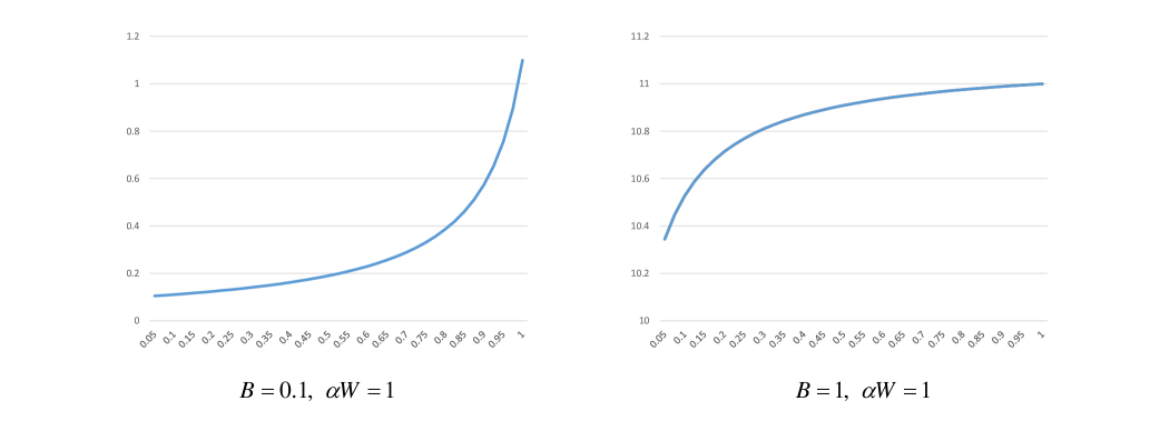
Figure 1: Plots of the equivalent bandwidth $T_{i}$ in (12) versus $\alpha$ with fixed average bandwidth $\alpha W$.

2.3 Welfare Measures

We will focus on two basic welfare measures, consumer surplus and social welfare. The consumer surplus associated with an equilibrium allocation is the difference between the amount the customers receiving service would be willing to pay and the total cost they incur. Since all customers incur the same cost $p_{d}$, it follows that the consumer surplus is given by

$$CS(z)=\int_{0}^{z}(P(y)-P(z))\,dy=\frac{z^{2}}{2}.\\$$ (13)

where $z$ denotes the total number of customers served over all bands. Note that $CS(z)$ is a strictly increasing function of $z$ so that to compare the consumer welfare of different equilibria we need only compare the number of customers served. The social welfare of an equilibrium is the sum of the consumer surplus and the total revenue earned by all SPs.

3 Two Service Providers

We start with the scenario in which there are two competing SP. This allows an illustration of the basic properties of the model. We then consider scenarios with more than two SPs in the subsequent section.

3.1 Shared Licensed Access

We first examine the scenario in which all of the shared bandwidth is available for licensed access. From Lemma 2.2, we can view each provider $i$ as having $T_{i}$ units of proprietary spectrum, which includes its portion of the shared spectrum. For $N=2$, the conditions for Cournot competition reduce to:

$$p_{d} =1-x_{1}-x_{2}$$

$$p_{1} =p_{d}-\frac{x_{1}}{T_{1}}=1-x_{1}\left(1+\frac{1}{T_{1}}\right)-x_{2}$$

$$p_{2} =p_{d}-\frac{x_{1}}{T_{2}}=1-x_{2}\left(1+\frac{1}{T_{2}}\right)-x_{1}$$

where the SPs choose $x_{1}$ and $x_{2}$, respectively. SP $i$’s revenue is given by $R_{i}=p_{i}x_{i}$, which from these relations is a quadratic funciton of $x_{i}$.

The next result characterizes the unique Nash equilibrium for this setting. We show in Theorem 6.1 that the underlying game is a potential game. From Lemma 2.2, the model reduces to an equivalent model with no intermittent spectrum, which corresponds to a special case of the model studied in [8].

THEOREM 3.1

There is a unique Nash equilibrium given by

$$x_{1}^{*} =\frac{T_{1}T_{2}+2T_{1}}{3T_{1}T_{2}+4+4(T_{1}+T_{2})}$$

$$x_{2}^{*} =\frac{T_{1}T_{2}+2T_{2}}{3T_{1}T_{2}+4+4(T_{1}+T_{2})}$$

with the equilibrium prices given by

$$p_{1}^{*} =\frac{T_{1}T_{2}+2T_{1}+T_{2}+2}{3T_{1}T_{2}+4+4(T_{1}+T_{2})}$$

$$p_{2}^{*} =\frac{T_{1}T_{2}+2T_{2}+T_{1}+2}{3T_{1}T_{2}+4+4(T_{1}+T_{2})}.$$

This theorem enables us to deduce the following comparitive statics.

THEOREM 3.2

Let $R_{i}(T_{1},T_{2})$ be the equilibrium revenue of SP $i\in\{1,2\}$ given that each SP $i$ has $T_{i}$ units of equivalent proprietary spectrum.

1. $R_{1}(T_{1},T_{2})$ is strictly increasing and concave in $T_{1}$ holding $T_{2}$ fixed.

2. $\frac{\partial R_{1}}{\partial T_{2}}<0$ .

3. If $T_{1}>T_{2}$, then $\frac{\partial R_{1}}{\partial T_{1}}>\frac{\partial R_{2}}{\partial T_{2}}$.

Theorem 3.2 has two immediate implications. First, unsurprisingly, each SP would prefer to have larger amounts of the equivalent shared bandwidth than not, other parameters held fixed. Second, an increase in the equivalent shared bandwidth of one’s rival results in a decrease in one’s own revenue. Interestingly, because $T_{i}$ increases with $B_{i}$, the marginal value of additional equivalent licensed bandwidth is larger for the SP with the larger initial amount of bandwidth.

From (13) the consumer surplus is given by

$$CS(z)=\frac{(x^{*}_{1}+x^{*}_{2})^{2}}{2},$$ (14)

and from Theorem 3.1 we have

$$x_{1}^{*}+x_{2}^{*} =\frac{T_{1}T_{2}+2T_{1}}{3T_{1}T_{2}+4+4(T_{1}+T_{2})}+\frac{T_{1}T_{2}+2T_{2}}{3T_{1}T_{2}+4+4(T_{1}+T_{2})}$$

$$=\frac{2T_{1}T_{2}+2(T_{1}+T_{2})}{3T_{1}T_{2}+4+4(T_{1}+T_{2})}.$$ (15)

Referring to the expression for $T_{i}$ in (12), consumer surplus is therefore a non-linear function of $W_{1},W_{2}$. This means that for some parameter settings consumer surplus will not be maximized by setting $W_{1}=W$ or $W_{2}=W$. To understand the implication of this suppose the incumbent decides to allocate all $W$ units of new bandwidth by auction to the highest bidder. The resulting allocation need not maximize consumer surplus. If $B_{1}=B_{2}$, then one can show that the new spectrum should be divided equally between the two SPs to maximize consumer welfare. In general, the allocation that maximizes consumer surplus will make the $T_{i}$ of the SP with the larger $B_{i}$ larger than the $T_{i}$ of the other SP (though the smaller SP may still get a larger amount of $W_{i}$). It is also the case that the SP with the larger $B_{i}$ benefits more from an increase in spectrum that is intermittent. (The smaller $\alpha$ is, the greater the difference in benefit.) This is because the larger SP is better able to absorb the fluctuations.

3.2 Shared Open Access

We now assume that each SP has its own proprietary bandwidth and that the additional shared bandwidth $W$ is open access. We begin with the symmetric case where each SP has the same amount of proprietary bandwidth, i.e., $B_{1}=B_{2}=B/2$.

THEOREM 3.3

When $B_{1}=B_{2}=B/2$ the unique Nash equilibrium is given by the quantities

$$x_{i}^{*} =\frac{\frac{3}{W}}{\frac{9}{W}+\frac{12}{B}+\frac{12}{BW}+\frac{16(1-\alpha)}{B^{2}}}=\frac{3B^{2}}{9B^{2}+12BW+12B+16(1-\alpha)W}$$

$$w_{i}^{*} =\frac{\frac{4}{B}}{\frac{9}{W}+\frac{12}{B}+\frac{12}{BW}+\frac{16(1-\alpha)}{B^{2}}}=\frac{4BW}{9B^{2}+12BW+12B+16(1-\alpha)W}.$$

for $i=1,2$.

In particular, both SPs make use of the unlicensed bandwidth. Direct computation using the preceding quantities shows that both SP revenue and consumer surplus increase with the following parameter variations:

1. $B$ increases holding $W$ and $\alpha$ fixed;

2. $W$ increases holding $B$ and $\alpha$ fixed;

3. $\alpha$ increases holding $B$ and $W$ fixed.

We remark that for the analogous Bertrand model considered in [6], the SP revenue generally decreases as $W$ increases. This is due to the shift in customers to the open access band, where the equilibrium price is zero. In contrast, for the Cournot model the corresponding shift in traffic generally lowers the price, but that is offset by an increase in the number of customers served.

We next consider the asymmetric scenario in which $B_{1}\neq B_{2}$. As $B_{1}$ increases relative to $B_{2}$ we obtain the following result.

THEOREM 3.4

Suppose that a fraction $\beta W$ of the shared bandwidth is provisioned as open access, and the remainder is partitioned as $W_{i}$, $i=1,2$, and allocated as licensed bandwidth to the respective SPs, where $\beta\in[0,1]$ and $W_{1}+W_{2}=(1-\beta)W$. Then, there is a unique equilibrium with $w_{1}^{*}=0$, $x_{1}^{*}>0$ and $x_{2}^{*}>w_{2}^{*}>0$ if and only if

$$B_{1}+W_{1}+2(1-\alpha)\frac{W_{1}}{B_{1}}\geq 2(\beta W+W_{2})+2B_{2}+2+4(1-\alpha)\frac{\beta W+W_{2}}{B_{2}}.$$ (16)

For $\beta=1$, all the shared bandwidth is open access and condition (16) simplifies to $B_{1}\geq 2W+4(1-\alpha)\frac{W}{B_{2}}+2B_{2}+2$.

Hence, if an SP has an amount of proprietary bandwidth that greatly exceeds that held by the other SP, there is a range of $W$ for which it will not make use of the shared bandwidth, leaving it for the smaller SP. Interestingly, as $\alpha$ decreases, i.e., the shared band is more likely to be pre-empted, the ‘larger’ SP is more likely to use it. This is because its proprietary bandwidth makes it better able to handle the traffic in the event of pre-emption.

The proof is given as part of Appendix 8.8 (see section 8.8.4). There it is also shown that conditioned on the shared spectrum being available,

$$\frac{x_{i}^{*}}{B_{i}+W_{i}}\leq\frac{w_{i}^{*}+\frac{w_{-i}^{*}}{2}}{\beta W}\leq\frac{w_{1}^{*}+w_{2}^{*}}{\beta W},$$

for $i\in\{1,2\}$, and where $-i$ denotes the other SP. Suppose that $\beta=1$, so that $W_{i}=0$. The condition then states that when the shared band is available, the congestion in the proprietary bands is always less than the congestion in the open access band. If SP $i$ uses the shared band, it is shown that the first inequality is tight. Additionally, if in equilibrium $w_{i}^{*}>0$ for both SPs, then for SP $i$ the congestion in the open access band is strictly greater than the congestion in its licensed bands by ${w_{-i}^{*}}/{(2W)}$. Furthermore, if in equilibrium $w_{i}^{*}=0$, then the open access band and proprietary band for the other provider $-i$ have the same congestion level, which is at least twice the congestion in SP $i$’s proprietary band. It is this additional congestion which causes SP $i$ to assign $w_{i}=0$, and to use only its proprietary bands. The appendix also considers $N>2$ asymmetric SPs, and gives a condition for when all but one SP assigns traffic to the open access band.

3.3 Numerical Examples

To illustrate the behavior of the SPs in scenarios not covered by Theorem 3.4 we present a series of numerical examples showing comparative statics with different assumptions concerning how the shared bandwidth is allocated.

Quantities and prices:

Figure 2 illustrates how quantities and prices in the shared and proprietary bands change as the amount of proprietary bandwidth for SP 1 ($B_{1}$) increases. Figure 2(a) shows that as $B_{1}$ increases, SP 1 increases the quantity of customers $x_{1}$ served in its proprietary band, and decreases its allocation of customers $w_{1}$ to the shared band. SP 2 maintains nearly constant quantities in both bands. The vertical line shows the threshold $B_{1}^{*}$ at which $w_{1}$ becomes zero. For $B_{1}>B_{1}^{*}$ the quantities are nearly constant with only slight variations due to the limited competition with only two SPs.

Figure 2(b) shows that SP 1 charges higher prices than SP 2 in both bands since it is able to provide lower latency than SP 2. For $B_{1}<B_{1}^{*}$, SP 1’s prices increase, due to decreasing latency, whereas SP 2’s prices decrease to maintain its quantity of customers. For $B_{1}>B_{1}^{*}$, $p_{1}$ increases slowly, since latency in that band continues to decrease, whereas the remaining prices decrease to maintain the nearly constant quantities shown in Figure 2(a).

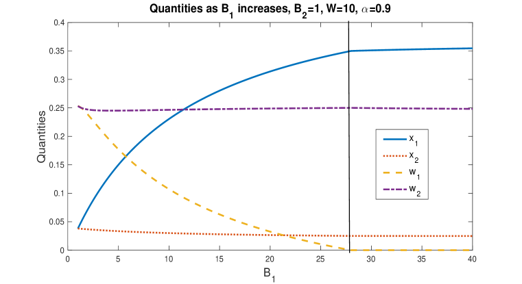
(a) Quantities

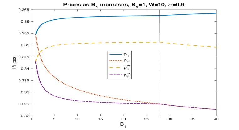
(b) Prices

Figure 2: Equilibrium quantities $x_{i}$, $w_{i}$, and prices $p_{i}$, $p_{i}^{w}$, $i=1,2$, as $B_{1}$ increases with $B_{2}=1$, $W=10$ and $\alpha=0.9$.

Social welfare:

Figure 3 shows social welfare achieved by four different schemes for allocating the shared spectrum. These schemes are motivated by the discussion following Theorem 3.2, which considers the outcome of a winner-take-all auction of the shared band. The label “SP 1” in Figure 3 indicates all of the shared spectrum is allocated to SP 1, which always possesses the greater amount of proprietary spectrum. Similarly, the label “SP 2” allocates all of the shared spectrum to SP 2. We compare the social welfare for these outcomes with that obtained by allocating the shared spectrum as open access, labeled “Open access”. Finally, the label “Split” allocates the shared spectrum to equalize the equivalent always-available bandwidths $T_{1}$ and $T_{2}$, if possible, or otherwise allocates all of the shared bandwidth to SP 2.

Figure 3(a) depicts how social welfare changes as a function of $B_{1}\geq B_{2}=1$ (with $\alpha=0.9$ and $W=10$). Assigning $W$ to the smaller provider SP 2 always achieves higher social welfare since this enables SP 2 to compete more effectively with SP 1. However, as implied by Theorem 3.2, SP 1 has an incentive to bid a higher amount for $W$ than SP 2. The resulting loss in social welfare is indicated in the figure. This analysis suggests that an auction for $W$ should be enhanced to contain more options. An example is provided in Appendix 8.1, which considers the scenario in which the SPs can bid for the shared spectrum with the following options: it is licensed entirely to SP 1 or SP 2, or it is shared as open access. The example shows that both SPs may prefer that the shared bandwidth be open access rather than licensed.

For the schemes considered in Figure 3, open access sharing yields the highest social welfare except for a small region where the scheme “SP 2” does marginally better. The “Vacate flag” indicates the values of $B_{1}$ for which SP 1 does not use the shared spectrum, so that it is effectively allocated to SP 2. Hence in that region the social welfare for open access coincides with that for scheme SP 2.

When it is possible to set $T_{1}=T_{2}$, the “Split” scheme achieves a higher social welfare than either scheme SP 1 or SP 2. This indicates that among schemes that partition the shared spectrum between the two SPs, there is an optimal split that lies between the two extreme schemes SP 1 and SP 2. Open access sharing can be thought of as a more flexible split between the two SPs. Figure 3(b) depicts how social welfare changes as $W$ increases for the four allocation schemes considered. The relative differences observed previously also apply in this regime. However, for open access sharing, as $W$ increases, in equilibrium, SP 1 always uses the shared spectrum.

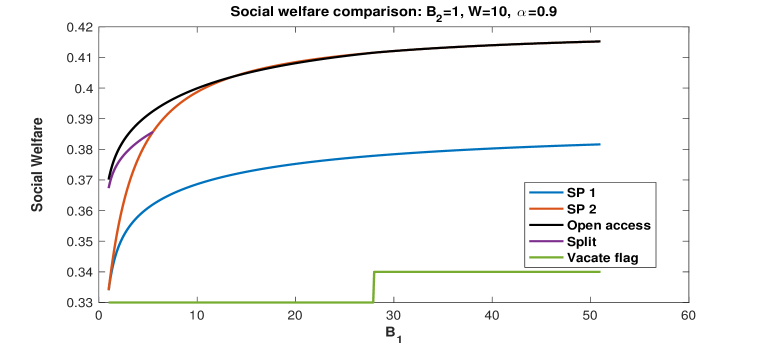
(a) $B_{1}$ varies with $W=1$

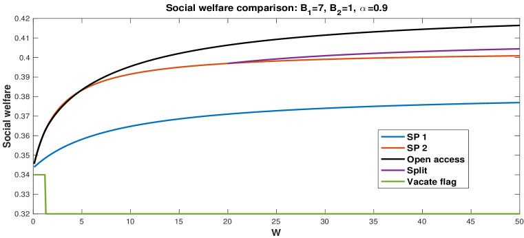
(b) $W$ varies with $B_{1}=7$

Figure 3: Comparison of social welfare for various schemes for allocating the shared bandwidth $W$; $B_{2}=1$ and $\alpha=0.9$.

4 Many Symmetric Service Providers

We now examine the scenario with an arbitrary number of SPs $N$, where the SPs are symmetric. That is, they each have the same amount of licensed bandwidth (including licensed shared bandwidth). Specifically, the shared band is split into an open access part with bandwidth $\beta W$ and a licensed, or proprietary part with bandwidth $(1-\beta)W$ for a fixed $\beta\in[0,1]$. Each SP has its own proprietary bandwidth $B/N$, and the licensed part of the shared band is split equally among the SPs. The shared band therefore adds $(1-\beta)W/N$ units of licensed bandwidth to each SP with availability $\alpha$. We will compare the total welfare, total revenue, and consumer surplus when the shared band is allocated as licensed versus open access. Analytical results are presented for $N\to\infty$, reflecting perfect competition.

Let $(\bar{x}(N),\bar{w}(N))$ denote the symmetric equilibrium allocation, i.e., $\bar{x}(N)$ and $\bar{w}(N)$ are the same for all SPs. Here $\bar{x}$ and $\bar{w}$ refer, respectively, to the quantities allocated to the licensed bands, including the licensed part of the shared band, and the open access band.

Lemma 4.1

For any finite $N$ the equilibrium is symmetric and unique.

THEOREM 4.2

As $N\to\infty$, the limiting equilibrium is specified by

$$(x^{*},w^{*})=\lim_{N\rightarrow\infty}(N\bar{x}(N),N\bar{w}(N)),$$

where

$$\begin{split}x^{*}&=\frac{\big{(}B+(1-\beta)W\big{)}B}{\big{(}B+2(1-\alpha)\big{)}\big{(}B+W(1+\beta)\big{)}+2B\alpha},\\ w^{*}&=\frac{2\beta WB}{\big{(}B+2(1-\alpha)\big{)}\big{(}B+W(1+\beta)\big{)}+2B\alpha},\end{split}$$ (17)

and the limiting prices in the licensed and open access bands are given by

$$\begin{split}p&=\frac{(1-\alpha)\big{(}B+W(1+\beta)\big{)}+B\alpha}{\big{(}B+2(1-\alpha)\big{)}\big{(}B+W(1+\beta)\big{)}+2B\alpha},\\ p^{w}&=\frac{(1-\alpha)\big{(}B+W(1+\beta)\big{)}}{\big{(}B+2(1-\alpha)\big{)}\big{(}B+W(1+\beta)\big{)}+2B\alpha}.\end{split}$$ (18)

The proof is given in Appendix 8.5. There the expressions for $\bar{x}(N)$, $\bar{w}(N)$ are given for arbitrary $N$.

Theorem 4.2 has the following implications.

1. From (18) $p>p^{w}$ for all $\alpha>0$. Also, from (17), the congestion, or load in the open access band (users/total bandwidth) is

   $$\frac{w^{*}}{\beta W}=2\frac{x^{*}}{B+(1-\beta)W}.$$ (19)

   Therefore, as $N\to\infty$, the congestion in the open access band is twice the congestion in the licensed/proprietary band, and the announced price for the open access band is lower than that for the licensed band. That is because the SPs have an incentive to shift traffic into the open access band, and then charge a higher price for the lower latency experienced in the licensed band. More generally, for arbitrary $N$, the expressions in the appendix show that the congestion in the open access band is $2N/(N+1)$ times the congestion in the proprietary bands.

2. Unlike the classical Cournot model of competition, the prices do not converge to zero as the number of competing agents becomes large. This is due to the tradeoff between announced price and congestion cost.

3. In the special case where the shared band is always available, $\alpha=1$ and

   $$\begin{split}p&=\frac{1}{W(1+\beta)+B+2},\;p^{w}=0.\end{split}$$ (20)

   That is, the price for the open access band is zero. This is analogous to the equilibrium with Bertrand (price) competition, derived in [6]. There it is also observed that the price of the open access band is zero, although here that occurs only when there are sufficiently many SPs.

THEOREM 4.3

As $N\rightarrow\infty$, consumer surplus is maximized when $\beta=1$. However, total revenue and social welfare are maximized when $\beta=0$.

From (17), the total traffic carried is given by

$$x^{*}+w^{*}=\frac{B\big{(}B+W(1+\beta)\big{)}}{\big{(}B+2(1-\alpha)\big{)}\big{(}B+W(1+\beta)\big{)}+2B\alpha}.$$

Hence the total traffic along with consumer surplus is maximized when $\beta=1$. The rest of the proof is given in Section 8.6.

Figure 4 illustrates the change in social welfare that takes place as $N$ increases. The plots show social welfare versus $N$ for both $\beta=0$ (all licensed) and $\beta=1$ (all open access), and for different values of $W$. Focusing on the bottom two curves for $W=1$, the curves cross when $N\leq 3$, i.e., for $N<3$, open access achieves higher social welfare than licensed access, and vice versa for $N>3$. This is consistent with Theorem 4.3. Note that the corresponding crossover value of $N$ increases as $W$ increases.

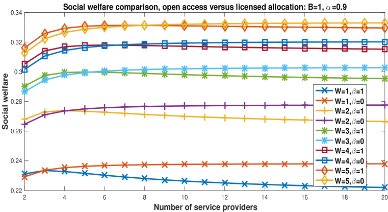
Figure 4: Social welfare achieved for $\beta=0$ and $\beta=1$ as a function of the number of (symmetric) SPs $N$ for different values of $W$. The total proprietary bandwidth $B=1$ and $\alpha=0.9$

4.1 Degraded Sharing

So far we have assumed that the latency experienced by serving traffic load $x$ with bandwidth $W$ is $x/W$ regardless if the traffic load comes from a single SP or multiple SPs. In practice, because less coordination is expected among SPs in the open access band, it could be that the latency experienced for a given load in the open access band is greater than if the same load were served by a single SP. That would make licensed access more attractive and with enough degradation, the conclusion of Theorem 4.3 that open access maximizes consumer surplus may no longer hold. In this section we examine this possibility.

We model the degradation associated with open access by introducing a degradation factor $d\leq 1$ and assume that when traffic load $x$ is served with open access bandwidth $W$, that the congestion cost is

$$\ell_{W}(x)=\frac{x}{dW}.$$

In other words, the “effective bandwidth” seen by the users of an open access band is $dW<W$. (Equivalently, the latency increases by $1/d$.)

Lemma 4.4

In the symmetric model with $N\geq 2$ firms, if $d>\frac{N+1}{2N}$, allocating all of the shared spectrum as open access maximizes consumer welfare, whereas if $d<\frac{N+1}{2N}$, allocating all of the shared spectrum as licensed maximizes consumer welfare.

The proof is given in Appendix 8.5.1, and is a consequence of the first property following Theorem 4.2. Note that the threshold $\frac{N+1}{2N}$ does not depend on $\alpha$, $W$ or $B$. This threshold is $3/4$ when $N=2$ and decreases to $1/2$ as $N$ becomes large. Hence for large $N$, unless the latency in the open access spectrum is more than twice that for licensed use due to lack of coordination, given the same load, open access still achieves larger consumer surplus.

4.2 Latency, price, and social welfare

To gain further insight into the effects of open access bandwidth on latency and price, Figures 5(a) and 5(b) show parametric plots of average price, consumer surplus, and total welfare versus average latency as the fraction of open access bandwidth $\beta$ increases from zero to one. The average price is given by Lemma 2.1, and the average latency is similarly

$$\bar{\ell}(N)=\frac{\bar{x}(N)}{\bar{x}(N)+\bar{w}(N)}\bar{\ell}_{p}(N)+\frac{\bar{w}(N)}{\bar{x}(N)+\bar{w}(N)}\bar{\ell}_{w}(N)$$ (21)

where

$$\bar{\ell}_{p}(N)=\alpha\frac{N\bar{x}(N)}{B+(1-\beta)W}+(1-\alpha)\frac{N(\bar{x}(N)+\bar{w}(N))}{B}$$ (22)

and

$$\bar{\ell}_{w}(N)=\alpha\frac{N\bar{w}(N)}{\beta W}+(1-\alpha)\frac{N(\bar{x}(N)+\bar{w}(N))}{B}$$ (23)

are the latencies associated with the proprietary and shared bands, respectively. The figure shows plots for $N=200$ and $N=2$, and $\alpha=1$.

No sharing ($\beta=0$) corresponds to the lowest latency on each curve (left-most point), and as $\beta$ increases from zero to one, the latency increases to the highest value (right-most point), and then subsequently decreases to the final point corresponding to full sharing ($\beta=1$). Focusing on Fig. 5(a), as $\beta$ increases from zero, the average price increases slightly as latency increases. This is because when $\beta W$ is small, the shift in load from the proprietary to shared band congests the shared band, increasing both average latency and price. In this region the consumer surplus and total welfare decrease. As $\beta$ increases further, the SPs lower the price to continue to shift load to the shared band, and the average latency continues to increase. In this region the consumer surplus increases while the total welfare continues to decrease due to the decrease in SP revenue. Finally, as $\beta$ is further increased towards one, both the price and latency fall, and consumer surplus increases more rapidly, causing total welfare to increase. Even so, the total welfare with full sharing is slightly below that with no sharing, as expected from Theorem 4.3.

Comparing Figure 5(a) with 5(b), the additional competition with $N=200$ results in a lower price and higher consumer surplus. Furthermore, the increase in open access bandwidth has a more pronounced effect on the quantities shown. Further examples with $\alpha<1$ show consistent trends, but with less variation with latency due to the diminished benefit of adding the shared bandwidth.

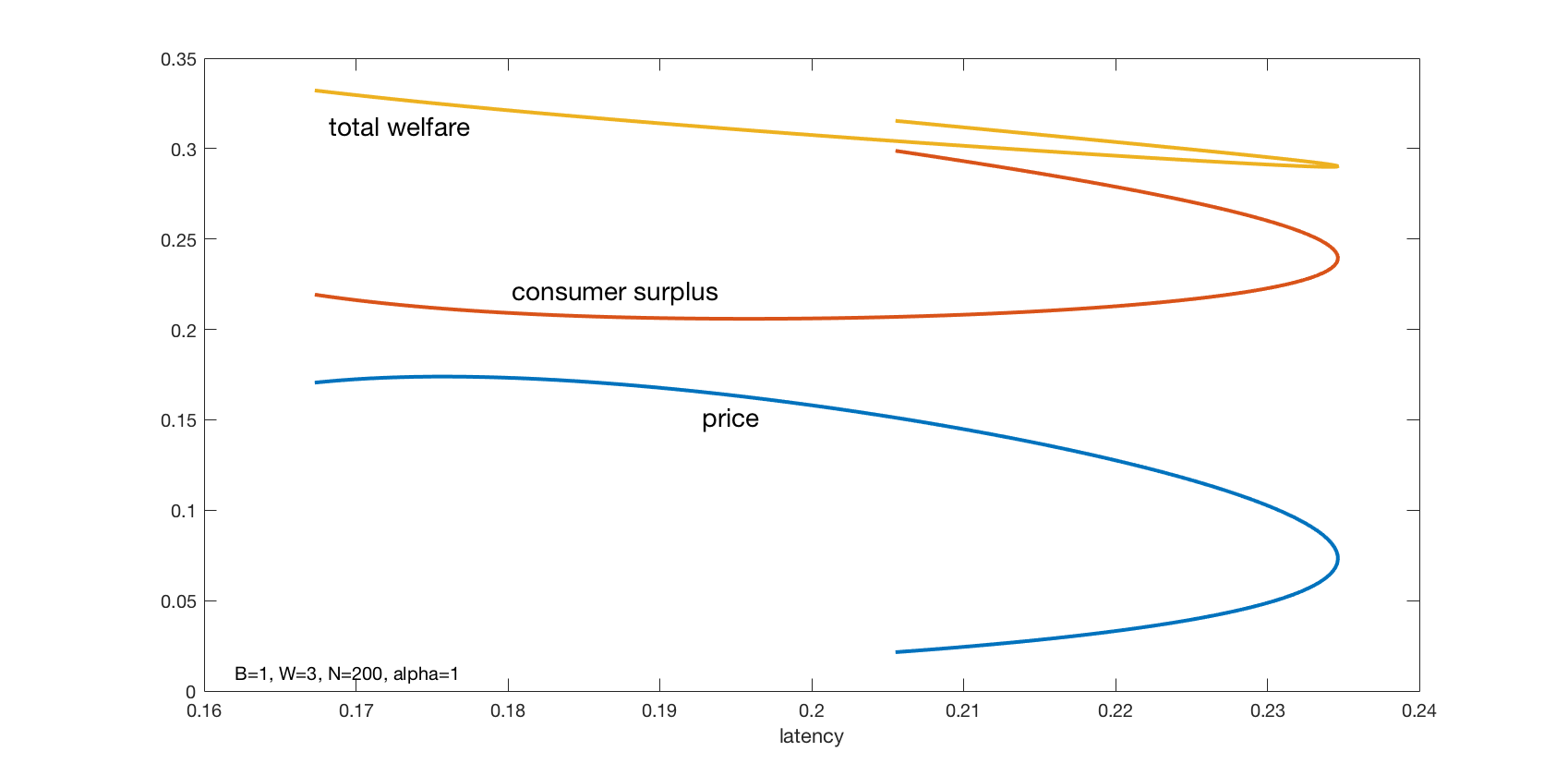
(a) $N=200$

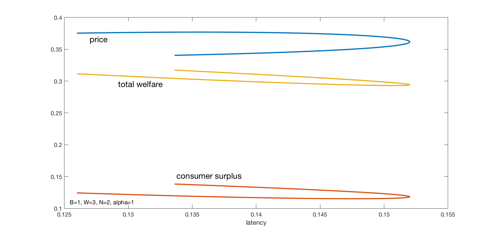
(b) $N=2$

Figure 5: Parametric plots of average price, consumer surplus, and total welfare versus average latency as the fraction of shared bandwidth $\beta$ increases from zero to one.

4.3 Effects of Increasing $W$

Fig. 6 illustrates the effect of increasing $W$ on social welfare, consumer surplus, and revenue for large $N$. Social welfare is shown for the cases where the shared bandwidth is entirely open access ($\beta=1$) and proprietary ($\beta=0$). Both curves are monotonically increasing, but their shape changes from convex to concave when the shared bandwidth changes from open access to proprietary. In particular, the slope at $W=0$ is zero when the shared band is open access, but is positive when the shared band is proprietary. This behavior has also been observed within the Bertrand model of price competition [6]. There, with a small number of SPs, adding a small amount of open access bandwidth can decrease the social welfare (i.e., the slope at $W=0$ can be negative). Here the additional incremental shared bandwidth increases social welfare for smaller values of $N$ (not shown), but the increase tends to zero as $N$ becomes large. The curves for revenue and consumer surplus displayed in Figure 6 correspond to open access. Here revenue decreases, but for $\beta=0$ the revenue initially increases slightly as $W$ increases from zero (not shown).

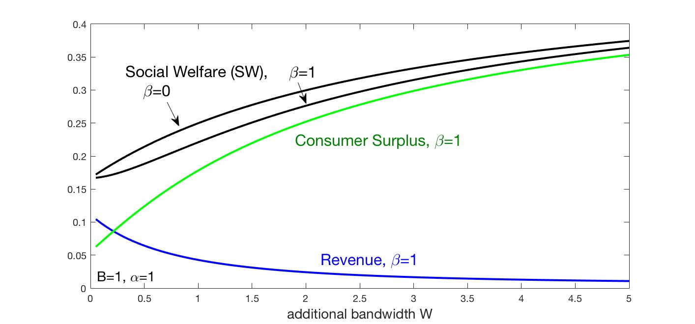
Figure 6: Total welfare versus additional bandwidth $W$ with a large number of SPs when the shared band is open access ($\beta=1$) and proprietary ($\beta=0$). Revenue and consumer surplus are also shown for $\beta=1$.

We can obtain further insight by letting $W$ become large. In this limit, some of the expressions simplify, easing the analysis. For a given number of SPs $N$, taking this limit and using the equilibrium expressions in the appendices, the total mass of customers served is given by

$$\rho(N)=\bar{x}(N)+\bar{w}(N)=\frac{B}{B+B/N+2(1-\alpha)}.$$

This does not depend on $\beta$ and so if there is sufficient shared bandwidth, it does not matter how it is allocated. The social welfare for licensed and open access shared bandwidth therefore become the same as illustrated in Fig. 6. This is intuitive since as $W\rightarrow\infty$ the congestion externality disappears in the shared spectrum, so open access and licensed access provide the same value to consumers. Note that $\rho(N)$, and hence consumer welfare, increases with $N$ and approaches the asymptote

$$\bar{\rho}=\frac{B}{B+2(1-\alpha)}.$$

In the limit of large $W$, the social welfare as a function of $N$ is given by

$$SW(N) =\rho(N)-\frac{\rho^{2}(N)}{2}\left(1+\frac{2(1-\alpha)}{B}\right).$$

This expression is an increasing function of $\rho(N)$ for $\rho(N)\leq\bar{\rho}$. Hence, $SW(N)$ is also increasing with $N$ and approaches the limiting value

$$\frac{B}{2(B+2(1-\alpha))}=\frac{\bar{\rho}}{2}.$$

Note that $\bar{\rho}$ is a strictly increasing function of $\alpha\in[0,1]$ and for $\alpha=1$, we have $\bar{\rho}=1$, meaning the entire market is served, resulting in a social welfare of $\frac{1}{2}$, which is the maximum possible for the assumed inverse demand. For $\alpha<1$, we have $\bar{\rho}<1$, meaning that even with an unbounded amount of shared spectrum, some users are not served due to the intermittent nature of that spectrum, so that some potential welfare is not obtained.

As previously noted for arbitrary $W$, the previous results show that when $\alpha<1$ and $N\rightarrow\infty$, the aggregate profit of the SPs is strictly positive. In this case, the limiting aggregate firm profit is given by

$$\bar{\rho}-\bar{\rho}^{2}\left(1+\frac{(1-\alpha)}{B}\right)=\frac{B(1-\alpha)}{(B+2(1-\alpha))^{2}}.$$

Differentiating this with respect to $\alpha$, it can be seen that for $B<2$, the aggregate firm profit first increases with $\alpha$ and then decreases, with the maximum firm profits occurring when $\alpha=1-B/2$. For $B\geq 2$, aggregate firm profits decrease with $\alpha$, and so the maximum occurs when $\alpha=0$. In other words, given any value of $B$, the SPs would prefer that the shared spectrum is intermittent, and if $B$ is large enough, they would prefer that the shared spectrum is never available. Adding new spectrum to the market reduces congestion, but also intensifies competition. The latter effect becomes more pronounced the less intermittent the spectrum becomes and apparently dominates the impact on the providers’ profits.

5 Asymmetric Providers

To provide insight into the effects of asymmetric (large and small) SPs with different amounts of bandwidth, we now consider the following two scenarios:

• There is a single SP with proprietary bandwidth $B_{1}$. A second band $B_{2}$ is split evenly among $N$ small SPs, where $N$ is assumed to be large.

• Bands $B_{1}$ and $B_{2}$ are each split among $N$ SPs. We will assume that $B_{1}\geq B_{2}$.

Varying $B_{1}$ relative to $B_{2}$ then captures varying degrees of asymmetry. The two scenarios differ in the amount of competition experienced by the SP(s) with the larger bandwidth allocation.

As before, the shared band is split between an open access part (bandwidth $\beta W$) and proprietary part (bandwidth $(1-\beta)W$). The open access part is shared among all SPs, large and small. The proprietary part is further split into two sub-bands with bandwidths $W_{1}$ and $W_{2}$ allocated to the large and small SPs, respectively. The shared band is intermittently available, so that a small SP has proprietary bandwidth $B_{2}/N$, which is always available, plus $W_{2}/N$, which is available with probability $\alpha$.

For the first scenario, let $x_{1}(N)$ and $w_{1}(N)$ denote the quantities served by the large SP in its proprietary and open access spectrum, respectively. The corresponding quantities for the $i^{\mathrm{th}}$ small SP are $x_{2,i}(N)$ and $w_{2,i}(N)$, respectively. By symmetry $x_{2,i}(N)$ and $w_{2,i}(N)$ are independent of $i$. As $N\to\infty$, the equilibrium quantities are defined as

$$(x_{1}^{*},w_{1}^{*},x_{2}^{*},w_{2}^{*})=\lim_{N\to\infty}[x_{1}(N),w_{1}(N),Nx_{2,i}(N),Nw_{2,i}(N)]$$ (24)

It is shown in Appendix 8.7 that those quantities are the solution to a set of four linear equations. Similarly, in the second scenario, $x_{1}(N)$ and $w_{1}(N)$ are replaced by $x_{1,j}(N)$ and $w_{1,j}(N)$, where $j$ denotes an SP in the larger group. From symmetry those quantities are independent of $j$, and as $N\to\infty$, the corresponding equilibrium quantities are

$$(x_{1}^{*},w_{1}^{*},x_{2}^{*},w_{2}^{*})=\lim_{N\to\infty}[Nx_{1,j}(N),Nw_{1,j}(N),Nx_{2,i}(N),Nw_{2,i}(N)]$$ (25)

As for the scenario with two asymmetric SPs, here also a larger SP does not always use the open access spectrum. In addition, for the second asymmetric scenario considered here with many larger SPs, a smaller SP may not use the open access spectrum. The associated conditions are stated next.

THEOREM 5.1

For the first scenario with asymmetric SPs, if

$$B_{1}+W_{1}+2(1-\alpha)\frac{W_{1}}{B_{1}}>2(1-\alpha)\frac{2\beta W+W_{2}}{B_{2}}$$ (26)

then there exists an $N^{*}$ such that for all $N\geq N^{*}$, SP 1 does not use the open access spectrum, i.e., $w_{1}^{*}(N)=0$.

For the second scenario, a larger (smaller) SP $i$ does not use the open access spectrum for all $N\geq N^{**}$ (for some $N^{**}$) when

$$\frac{W_{i}}{B_{i}}>\frac{2\beta W+W_{j}}{B_{j}},~{}~{}~{}i\neq j.$$ (27)

where $j$ corresponds to a smaller (larger) SP.

The proof can be found in Appendix 8.8.4.

The first condition (26) resembles, but is not identical to the condition in Theorem 3.4. This is because here a portion of the licensed spectrum is also intermittent. Note that for $\alpha=1$ the larger SP always vacates the open access spectrum. Also, for $\alpha=1$, the price in the shared spectrum is zero, which is also true for the analogous model with Bertrand competition [6]. The first condition in Theorem 5.1 is satisfied when $\beta$ and $W_{2}$ are small. In that case, the smaller SPs congest the open access band, lowering the price, and thereby make it less desirable for the large SP(s). For small $\beta$ the second condition (27) becomes $W_{i}/B_{i}>W_{j}/B_{j}$. If $W_{i}>W_{j}$, then the condition can be satisfied with $B_{i}<B_{j}$, i.e., the smaller SPs vacate the open access band. This is due to competition among the larger SPs, which causes them to shift traffic to the open access band, increasing congestion in that band and lowering the price so that the smaller SPs have no incentive to use it.

The condition (27) does not depend on $\alpha$, in contrast to (26), because for large $N$, the additional congestion caused by intermittency is bounded, and is shared among the $N$ large SPs. Hence that additional congestion does not significantly affect an individual SP. As $\alpha$ decreases, the threshold $N^{**}$ must increase in order for the condition to apply.

Fig. 7 illustrates how the split of the shared band $W$ into $W_{1}$ and $W_{2}$ affects consumer surplus. Here $B_{1}=0.9$, $B_{2}=0.1$, $W=2$, $\beta=0$ (all of $W$ is split between the SPs), and plots are shown for different values of $\alpha$. The figures show consumer welfare as a function of $W_{1}/W$ for $N=2$ (Fig. 7(a)) and $N=60$ (Fig. 7(b)). As $\alpha$ increases, Fig. 7(a) shows that the fraction of bandwidth that maximizes consumer surplus shifts to the left. This is due to the tradeoff between the larger SP’s ability to handle intermittent traffic, and competition. That is, when $\alpha$ is small, most of the shared band should be allocated to the larger SP, since the larger SP is better able to handle the intermittent availability of the shared band. As $\alpha$ increases, so that the band becomes more reliable, the consumer surplus increases by shifting bandwidth to the smaller SP to increase competition. In contrast, Fig. 7b shows that with many competing SPs it is always best to give most of the shared bandwidth to the larger SPs, independent of $\alpha$.

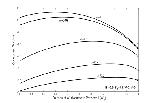
(a) $N=2$

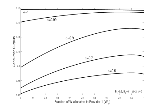
(b) $N=60$

Figure 7: Consumer surplus versus the fraction of shared bandwidth assigned to SP 1 ($W_{1}/W$) with different values of $\alpha$.

As for the symmetric case, numerical examples show that social welfare decreases with $\beta$ when $N\to\infty$, which is the same as for the symmetric case. In contrast, for $N=2$ the total welfare increases with $\beta$, as discussed in Section 3. Hence at these extreme values designating the entire band $W$ as open access ($N=2$) or proprietary ($N\to\infty$) maximizes total welfare. Additional numerical examples indicate that this is also true for arbitrary $N$.

6 Extensions to General Latency and Demand

In this section we establish existence of a unique equilibrium for the Cournot game with more general demand and latency functions. The model allows the shared band to be split between licensed and open access. When the shared band is available, the total licensed bandwidth of a SP changes and hence so does the latency cost experienced by customers served on the licensed band. In addition, with a linear inverse demand function, linear latencies in the open access bands and general convex increasing latencies in the licensed bands, we also prove that the game is a potential game. This fact is used in deriving some of our earlier results.

Assume that when the intermittent band is available, the latency function is given by $\ell_{i,w}(\cdot)$, and $\ell_{i}(\cdot)$ when not available.

THEOREM 6.1

For the Cournot game with $N\geq 2$ providers, each with proprietary spectrum and additional intermittently available shared spectrum, if the inverse demand $P(\cdot)$ is concave decreasing, and the latencies $\ell_{i}(\cdot)$, $\ell_{i,w}(\cdot)$ and $\ell_{w}(\cdot)$ are convex increasing, then an equilibrium always exists. The equilibrium is unique if either $P^{\prime}(0)<0$ and $\ell_{w}^{\prime}(0)>0$ or $\ell_{i}^{\prime}(0)>0$ and $\ell_{i,w}^{\prime}(0)>0$ for all $i=1,2,\dotsc,N$.

In the absence of open access spectrum, Theorem 6.1 holds without the condition on $\ell_{w}^{\prime}(\cdot)$ and $\ell_{i,w}^{\prime}(\cdot)$ for all $i=1,2,\dotsc,N$. When bandwidths $W_{1},W_{2},\dotsc,W_{N}$ with intermittent availability $\alpha$ are added, this is equivalent to the set of non-intermittent bands $T_{1},\cdots,T_{N}$, where $T_{i}$ is give in (12). With linear decreasing inverse demand, the existence and uniqueness of an equilibrium follows from Proposition 2 in [8].

We now assume two SPs with propriety spectrum only, i.e., any shared spectrum is licensed and always available, so that we can assume $W=0$. The proofs of the following propositions are in Appendix 8.9.

Proposition 6.2

Given an equilibrium (interior point) with two providers, concave decreasing inverse demand, and convex increasing latency, if a marginal amount of bandwidth is given to provider $k$, then a sequence of best responses converges to a new equilibrium in which the quantity $x_{k}$ and revenue $R_{k}$ each increase and $x_{-k}$ and $R_{-k}$ each decrease.

According to Theorem 6.1, the sequence of best responses must converge to a unique equilibrium. This extends Theorem 3.2, and states that in this more general setting an increase in one provider’s bandwidth again causes a decrease in the competitor’s quantity and revenue.

Proposition 6.3

For the scenario in Prop. 6.2, giving a marginal amount amount of bandwidth to SP $k$ increases both consumer surplus and total welfare.

This states that although from Proposition 6.2, adding this marginal bandwidth increases $x_{k}$ and decreases $x_{-k}$, the total quantity of customers served increases. Similarly, although the revenue $R_{-k}$ decreases, the total welfare increases.

Suppose now that we wish to give the bandwidth to the SP which will increase consumer surplus the most. That means allocating the bandwidth to maximize the total incremental quantity customers served. In general, this depends on the derivative $P^{\prime}(\cdot)$ and second derivative $\ell^{\prime\prime}(\cdot)$, and is somewhat complicated (see Appendix 8.9); however, for linear latencies $\ell_{k}(x)=c_{k}x$, it reduces to finding

$$\arg\max_{k}-\frac{c_{k}x_{k}}{B_{k}^{2}}\left(P^{\prime}(x_{1}+x_{2})-\frac{2c_{-k}}{B_{-k}}\right)$$ (28)

Further constraining $P(x)=1-ax$, and using the best response conditions for $x_{k}$, $x_{-k}$, the bandwidth should be given to agent $k$ if

$$B_{-k}>\sqrt{\frac{c_{-k}}{c_{k}}}B_{k}+\frac{2}{a}(\sqrt{c_{k}c_{-k}}-c_{-k})$$ (29)

Otherwise, it should be given to agent $-k$. Recall that when allocating additional intermittent spectrum ($\alpha<1$), the consumer surplus is given by (14)-(15). Here we effectively have $\alpha=0$ so that $T_{i}=B_{i}+W_{i}$, which replaces $B_{i}$ in the preceding condition. When $c_{k}=c_{-k}$ the condition reduces to $B_{-k}>B_{k}$, so that any marginal bandwidth should attempt to equalize the bandwidth allocation. If $c_{k}<c_{-k}$, however, the allocation is biased towards SP $k$, which provides lower latency.

7 Conclusions

We have presented a model for sharing intermittently available spectrum that captures licensed and open access sharing modes, congestion as a function of offered load, and competitive pricing for spectrum access. Our analysis suggests that allocating shared bandwidth as open access is better for consumer surplus than licensing the bandwidth for exclusive use. While latencies will be high, that is offset by lower prices, which has the effect of expanding the demand for services. Allocating additional bandwidth as licensed is good for revenue, because SPs generally choose to lower congestion by raising prices. The trade-off among revenue, consumer surplus, and congestion depends greatly on the market structure. With many SPs, competition may be enough so that total welfare (revenue plus consumer surplus) is maximized by licensing the intermittent bandwidth. With asymmetric SPs having different amounts of bandwidth, it is also possible that only a subset of the SPs use the open access band to maintain higher prices, thereby containing congestion.

The model might be enhanced in several different ways. We have not directly accounted for investment, which may be used to mitigate congestion, although we have shown that our main conclusions are robust with respect to a congestion penalty for open access. We have also generally assumed that access to the shared band is free, and have not considered pricing mechanisms, which could be used to allocate the shared spectrum as a combination of licensed and open access. Those features might also be combined with an extended model that allows SPs without proprietary spectrum to bid for open access spectrum, potentially combining both price and quantity competition.

8 Appendix

8.1 Bidding for shared spectrum: licensed versus open access

We consider the scenario in which two SPs can bid on the shared bandwidth $W$, and show that they may prefer that $W$ be allocated as open access rather than licensed. Assume that $B_{1}=B_{2}$, and that the incumbent of the shared band wishes to distribute $W=1$. It can offer it as open access or allocate it entirely to one of the providers. The table below records the revenue each provider makes under each possibility.

$\alpha$	pre-allocation	large	small	open access
0.1	0.08	0.096	0.052	0.063
0.5	0.08	0.102	0.057	0.068
0.9	0.08	0.11	0.064	0.075

The column labeled ‘pre-allocation’ lists the revenue of each SP before the allocation of additional bandwidth. The column labeled ‘large’ records the revenue of the SP that receives the entire one unit of additional bandwidth. The column labeled ‘small’ is the revenue of the SP who did not receive the additional bandwidth. The last column is the revenue of each SP when the additional unit of bandwidth is offered as open access. Each row corresponds to various levels of $\alpha$.

Consider, for example, the case $\alpha=0.5$. Suppose the one unit of additional bandwidth is allocated in its entirety via an ascending auction. If the current price is $p$, an SP should remain active provided:

$$0.102-p\geq 0.057\,\,\Rightarrow\,\,p\leq 0.045.$$

Hence, each SP should remain active until the price reaches 0.045. The winner will earn a profit of 0.102 - 0.045 = 0.057. Notice, the profit of each SP is higher in the open access regime. Hence, when paying for the additional bandwidth each SP would prefer open access sharing over having the additional bandwidth as licensed to themselves.

8.2 Proof of Theorem 3.1

Theorem 3.1 follows in the standard way by deriving the reaction functions of each provider and determining their intersection. Hence, many of the details are omitted. The revenue of provider $i$, denoted $R_{i}$ is:

$$p_{i}\left(1-x_{i}\left(1+\frac{1}{T_{i}}\right)-x_{-i}\right).$$

Compute $\partial R_{i}/\partial x_{i}$ for each $i$ and set to zero. The solution of this pair of first order conditions is unique. The corresponding equilibrium quantities and prices for provider 1 are

$$x_{1}^{*}=\frac{T_{1}}{T_{1}\frac{3T_{2}+4}{T_{2}+2}+\frac{4T_{2}+4}{T_{2}+2}},\quad p_{1}^{*}=\frac{T_{1}+1}{T_{1}\frac{3T_{2}+4}{T_{2}+2}+\frac{4T_{2}+4}{T_{2}+2}}$$

so that $x_{1}^{*}=\tfrac{T_{1}}{bT_{1}+a}$ and $p_{1}^{*}=\tfrac{T_{1}+1}{bT_{1}+a}$ where

$$b=\frac{3T_{2}+4}{T_{2}+2}=3-\frac{2}{T_{2}+2}\in[2,3),\quad a=\frac{4T_{2}+4}{T_{2}+2}=4-\frac{4}{T_{2}+2}\in[2,4)$$ (30)

8.3 Proof of Theorem 3.2

To prove Theorem 3.2, recall that the revenue of provider $1$ is given by $R_{1}^{*}=p_{1}^{*}x_{1}^{*}=\tfrac{T_{1}(T_{1}+1)}{(bT_{1}+a)^{2}}$ so that

$$\frac{\partial R_{1}}{\partial T_{1}} =\frac{(2T_{1}+1)(bT_{1}+a)-2bT_{1}(T_{1}+1)}{(bT_{1}+a)^{3}}=\frac{(2a-b)T_{1}+a}{(bT_{1}+a)^{3}}$$

$$\frac{\partial^{2}R_{1}}{\partial T_{1}^{2}} =\frac{(2a-b)(bT_{1}+a)-3b\big{(}(2a-b)T_{1}+a\big{)}}{(bT_{1}+a)^{4}}=\frac{-2b(2a-b)T_{1}-2a(2b-a)}{(bT_{1}+a)^{4}},$$

where $a$ and $b$ are defined in (30). Using the expressions for $a$ and $b$, we get

$$2a-b=5-\frac{6}{T_{2}+2}\in[2,5),\quad 2b-a=2.$$

Therefore, the revenue of provider $1$ is strictly concave and increasing in $T_{1}$ for any given value of $T_{2}$.

Both $b$ and $a$ are increasing in $T_{2}$ and so it follows that $R_{1}^{*}$ is decreasing in $T_{2}$.

8.4 Proof of Theorem 3.3

If an interior equilibrium exists, then:

$$p_{i} =1-x_{i}(1+\tfrac{1}{B_{i}})-x_{-i}-w_{i}(1+\tfrac{(1-\alpha)\beta}{B_{i}})-w_{-i}$$

$$p_{i}^{w} =1-x_{i}(1+\tfrac{1-\alpha}{B_{i}})-x_{-i}-w_{i}(1+\tfrac{\alpha}{W}+\tfrac{(1-\alpha)\beta}{B_{i}})-w_{-i}(1+\tfrac{\alpha}{W})$$

Using this, the revenue of provider $i$ is:

$$R_{i}=p_{i}x_{i}+p_{i}^{w}w_{i}$$

$$=(1-x_{-i}-w_{-i})x_{i}-x_{i}w_{i}(2+\tfrac{(1-\alpha)(1+\beta)}{B_{i}})-x_{i}^{2}(1+\tfrac{1}{B_{i}})+(1-x_{-i}-w_{-i}(1+\tfrac{\alpha}{W}))w_{i}$$

$$\qquad-w_{i}^{2}(1+\tfrac{\alpha}{W}+\tfrac{(1-\alpha)\beta}{B_{i}})$$

Assuming the revenue is jointly concave in $(x_{i},w_{i})$ (which is true for $\beta=1$ the case of interest), the best response functions are obtained by setting the following (partial) derivatives to $0$, namely,

$$\frac{\partial R_{i}}{\partial x_{i}} =1-x_{-i}-w_{-i}-w_{i}(2+\tfrac{(1-\alpha)(1+\beta)}{B_{i}})-2x_{i}(1+\tfrac{1}{B_{i}})$$

$$\frac{\partial R_{i}}{\partial w_{i}} =1-x_{-i}-w_{-i}(1+\tfrac{\alpha}{W})-x_{i}(2+\tfrac{(1-\alpha)(1+\beta)}{B_{i}})-2w_{i}(1+\tfrac{\alpha}{W}+\tfrac{(1-\alpha)\beta}{B_{i}}).$$

In the symmetric case of $B_{1}=B_{2}=B/2$, we search for a symmetric equilibrium using the above to get the following linear equations

$$x(3+\tfrac{4}{B})+w(3+\tfrac{2(1-\alpha)(1+\beta)}{B}) =1$$

$$x(3+\tfrac{2(1-\alpha)(1+\beta)}{B})+w(3+\tfrac{3\alpha}{W}+\tfrac{4(1-\alpha)\beta}{B}) =1$$

Solving this yields the quantities in the theorem. The resulting prices are

$$p_{1}=p_{2} =1-x(2+\tfrac{2}{B})-w(2+\tfrac{2(1-\alpha)}{B})$$

$$p_{1}^{w}=p_{2}^{w} =1-x(2+\tfrac{2(1-\alpha)}{B})-w(2+\tfrac{2\alpha}{W}+\tfrac{2(1-\alpha)}{B})$$

From the equations of the equilibrium, it can be gleaned that the prices are positive. Thus, an interior equilibrium exists.

8.5 Proof of Theorem 4.2.

For the analysis we assume that $\min\big{(}B+(1-\beta)W,\beta W\big{)}>0$. The results for the equilibrium quantities when this condition does not hold follow by continuity with the additional assumption that $B=0$ is necessarily accompanied with $\alpha=1$.

The revenue of SP $i$ is

$$R_{i}= p_{i}x_{i}+p_{i}^{w}w_{i}$$

$$= \left(1-\sum_{j=1}^{N}x_{j}-\sum_{j=1}^{N}w_{j}-\alpha N\frac{x_{i}}{B+(1-\beta)W}-(1-\alpha)N\frac{w_{i}+x_{i}}{B}\right)x_{i}$$

$$+ \left(1-\sum_{j=1}^{N}x_{j}-\sum_{j=1}^{N}w_{j}-\alpha\frac{\sum_{j=1}^{N}w_{j}}{\beta W}-(1-\alpha)N\frac{w_{i}+x_{i}}{B}\right)w_{i}$$

Taking the derivative of $R_{i}$ with respect to $x_{i}$

$$\frac{\partial R_{i}}{\partial x_{i}}= \left(1-\sum_{j=1}^{N}x_{j}-\sum_{j=1}^{N}w_{j}-\alpha N\frac{x_{i}}{B+(1-\beta)W}-(1-\alpha)N\frac{w_{i}+x_{i}}{B}\right)$$

$$\quad-\left(1+\alpha N\frac{1}{B+(1-\beta)W}+(1-\alpha)N\frac{1}{B}\right)x_{i}-(1+\frac{(1-\alpha)N}{B})w_{i}$$

We will derive a symmetric equilibrium. It will follow from a subsequent theorem, Theorem 6.1, that the unique equilibrium is symmetric. If we set $x_{i}=x$ and $w_{i}=w$ for all $i$, we get:

$$1= \left(Nx+Nw+\alpha N\frac{x}{B+(1-\beta)W}+(1-\alpha)N\frac{x+w}{B}\right)$$

$$\quad+\left(1+\alpha N\frac{1}{B+(1-\beta)W}+(1-\alpha)N\frac{1}{B}\right)x+(1+\frac{(1-\alpha)N}{B})w$$

This implies

$$1=x\left(1+N+2N\frac{\alpha}{B+(1-\beta)W}+2N\frac{(1-\alpha)}{B}\right)+w\left(1+N+2N\frac{1-\alpha}{B}\right)$$ (31)

Taking derivative with respect to $w_{i}$

$$\frac{\partial R_{i}}{\partial w_{i}}= -\left(1+\frac{(1-\alpha)N}{B}\right)x_{i}$$

$$+ \left(1-\sum_{j=1}^{N}x_{j}-\sum_{j=1}^{N}w_{j}-\alpha\frac{\sum_{j=1}^{N}w_{j}}{\beta W}-(1-\alpha)N\frac{w_{i}+x_{i}}{B}\right)-\left(1+\frac{\alpha}{\beta W}+\frac{(1-\alpha)N}{B}\right)w_{i}$$

Using an argument similar to that above we get

$$1=x\left(1+N+2N\frac{1-\alpha}{B}\right)+w\left(1+\frac{\alpha}{\beta W}+N+N\frac{\alpha}{\beta W}+2N\frac{1-\alpha}{B}\right)$$ (32)

Solving for the equilibrium using (31) and (32), we obtain

$$\bar{x}(N) =\frac{\frac{\alpha(N+1)}{\beta W}}{\Big{(}1+N+\frac{2(1-\alpha)N}{B}\Big{)}\Big{(}\frac{2\alpha N}{B+(1-\beta)W}+\frac{\alpha(N+1)}{\beta W}\Big{)}+\frac{2\alpha N}{B+(1-\beta)W}\frac{\alpha(N+1)}{\beta W}},$$

$$\bar{w}(N) =\frac{\frac{2\alpha N}{B+(1-\beta)W}}{\Big{(}1+N+\frac{2(1-\alpha)N}{B}\Big{)}\Big{(}\frac{2\alpha N}{B+(1-\beta)W}+\frac{\alpha(N+1)}{\beta W}\Big{)}+\frac{2\alpha N}{B+(1-\beta)W}\frac{\alpha(N+1)}{\beta W}}.$$

Rearranging we get

$$N\bar{x}(N) =\frac{B^{2}+(1-\beta)BW}{\left(B\frac{1+N}{N}+2(1-\alpha)\right)\left(2\beta W\frac{N}{N+1}+B+(1-\beta)W\right)+2\alpha B},$$ (33)

$$N\bar{w}(N) =\frac{2\beta BW\frac{N}{N+1}}{\left(B\frac{1+N}{N}+2(1-\alpha)\right)\left(2\beta W\frac{N}{N+1}+B+(1-\beta)W\right)+2\alpha B}.$$ (34)

The results then follow in a straight-forward manner by taking the limit as $N$ increases to infinity. We also note that the congestion in the shared band is exactly $\tfrac{2N}{N+1}$ times the congestion in the proprietary bands.  

8.5.1 Consumer Surplus

The total traffic carried $\rho(N)$ is then

$$\rho(N) =N\bar{x}(N)+N\bar{w}(N)$$

$$=\frac{B^{2}+\left(1+\beta\frac{N-1}{N+1}\right)BW}{\left(B\frac{1+N}{N}+2(1-\alpha)\right)\left(2\beta W\frac{N}{N+1}+B+(1-\beta)W\right)+2\alpha B}$$

$$=\frac{B\left(B+\left(1+\beta\frac{N-1}{N+1}\right)W\right)}{\left(B+\frac{B}{N}+2(1-\alpha)\right)\left(B+\left(1+\beta\frac{N-1}{N+1}\right)W\right)+2\alpha B},$$

which is of the form $\frac{af(\beta)}{(a+b)f(\beta)+c}$ where $f(\beta)$ is an increasing function of $\beta,$ and $a,b,c>0$. Therefore, it is immediate that $\rho(N)$ is also an increasing function of $\beta$, and so is maximized at $\beta=1$.

Next we present the proof of Lemma 4.4, which studies consumer surplus with degraded shared spectrum. When we allow the shared spectrum to get degraded, i.e., reduce by a factor $d$, then we can use the formulae in (33) and (34) to analyze the equilibrium by setting the shared bandwidth $\beta W$ to $d\beta W$. Define $d^{*}=\tfrac{2dN}{N+1}$. Then the congestion in the shared band is still $\tfrac{2N}{N+1}$ times the congestion in the proprietary band, i.e., denoting $(\bar{x}_{\beta}(N),\bar{w}_{\beta}(N))$ as the equilibrium quantities have the following expressions:

$$N\bar{x}_{\beta}(N) =\frac{B^{2}+(1-\beta)BW}{\left(B\frac{1+N}{N}+2(1-\alpha)\right)\left(2d\beta W\frac{N}{N+1}+B+(1-\beta)W\right)+2\alpha B},$$

$$N\bar{w}_{\beta}(N) =\frac{2d\beta BW\frac{N}{N+1}}{\left(B\frac{1+N}{N}+2(1-\alpha)\right)\left(2d\beta W\frac{N}{N+1}+B+(1-\beta)W\right)+2\alpha B},$$

$$\Leftrightarrow\quad\frac{N\bar{w}_{\beta}(N)}{d\beta W} =\frac{2N}{N+1}\frac{N\bar{x}_{\beta}(N)}{B+(1-\beta)W},$$

where we used the increased latency in the shared band for the comparison. Using this we have the total traffic served $\rho_{\beta}(N)$ is then

$$\rho_{\beta}(N) =N\bar{x}_{\beta}(N)+N\bar{w}_{\beta}(N)$$

$$=\frac{B\left(B+\left(1+\beta(d^{*}-1)\right)W\right)}{\left(B+\frac{B}{N}+2(1-\alpha)\right)\left(B+\left(1+\beta(d^{*}-1)\right)W\right)+2\alpha B},$$

which is an increasing function of $\beta$ if $d^{*}>1$ and a decreasing function of $\beta$ if $d^{*}<1$. This conclusion then directly implies that the consumer surplus is maximized at $\beta=1$ if $d^{*}>1$ and at $\beta=0$ if $d^{*}<1$.

8.5.2 Total Surplus

Assuming no degradation of the shared band the revenue of SP $i$ is

$$R_{i}= \left(1-N\bar{x}(N)-N\bar{w}(N)-\alpha N\frac{\bar{x}(N)}{B+(1-\beta)W}-(1-\alpha)N\frac{\bar{w}(N)+\bar{x}(N)}{B}\right)\bar{x}(N)$$

$$+ \left(1-N\bar{x}(N)-N\bar{w}(N)-\alpha\frac{N\bar{w}(N)}{\beta W}-(1-\alpha)N\frac{\bar{w}(N)+\bar{x}(N)}{B}\right)\bar{w}(N)$$

$$= \left(1-\rho(N)-\alpha N\frac{\bar{x}(N)}{B+(1-\beta)W}-(1-\alpha)\frac{\rho(N)}{B}\right)\bar{x}(N)$$

$$+ \left(1-\rho(N)-\alpha\frac{N\bar{w}(N)}{\beta W}-(1-\alpha)\frac{\rho(N)}{B}\right)\bar{w}(N)$$

Hence, total revenue is

$$(1-\rho(N))\rho(N)-\frac{(1-\alpha)}{B}\rho^{2}(N)-\frac{\alpha N^{2}\bar{x}(N)^{2}}{B+(1-\beta)W}-\frac{\alpha N^{2}\bar{w}(N)^{2}}{\beta W}.$$

As consumer surplus is $\frac{\rho(N)^{2}}{2}$ it follows that total surplus is

$$\rho(N)-\frac{\rho(N)^{2}}{2}-\frac{(1-\alpha)}{B}\rho^{2}(N)-\frac{\alpha N^{2}\bar{x}(N)^{2}}{B+(1-\beta)W}-\frac{\alpha N^{2}\bar{w}(N)^{2}}{\beta W}.$$

Plots for various parameter values suggest that social welfare is a convex function of $\beta$ for each $N$. If true, maximization over $\beta$ is achieved at one of the endpoints, i.e., either $0$ or $1$. The maximizer $\beta^{*}(N)$ is initially $0$, and it jumps to $1$ and remains there for large enough $N$. Most examples show this is between 2 and 3 (see Figure 4).

8.6 Proof of Theorem 4.3

Recall that the total traffic carried is given by

$$\rho:=x^{*}+w^{*}=\frac{B\big{(}B+W(1+\beta)\big{)}}{\big{(}B+2(1-\alpha)\big{)}\big{(}B+W(1+\beta)\big{)}+2B\alpha}.$$

It is straightforward to verify that the total quantity carried, and hence, the consumer surplus are both maximized at $\beta=1$.

Now social welfare as a function of $\beta$ denoted $SW(\beta)$ is given by:

$$SW(\beta)=\frac{(B+W+W\beta)^{2}(\frac{B^{2}}{2}+B(1-\alpha))+B^{2}\alpha(B+W-W\beta).}{\left[(B+W+W\beta)(B+2(1-\alpha))+2B\alpha\right]^{2}}.$$

The derivative of $SW(\beta)$ with respect to $\beta$ when set to zero has a unique solution, $\beta^{*}$. For $0\leq\beta<\beta^{*}$ the derivative is negative, for $\beta^{*}<\beta\leq 1$, it is positive. Thus to find the maximum value it is sufficient to compare the values at the two extremes. Now,

$$SW(0)=\frac{(B+W)^{2}(\frac{B^{2}}{2}+B(1-\alpha))+B^{2}\alpha(B+W)}{\left[(B+W)(B+2(1-\alpha))+2B\alpha\right]^{2}}$$

and

$$SW(1)=\frac{(B+2W)^{2}(\frac{B^{2}}{2}+B(1-\alpha))+B^{3}\alpha)}{\left[(B+2W)(B+2(1-\alpha))+2B\alpha\right]^{2}}.$$

Now $SW(0)>SW(1)$ implies

$$\frac{(B+W)^{2}(B+2(1-\alpha))+2B\alpha(B+W)}{\left[(B+W)(B+2(1-\alpha))+2B\alpha\right]^{2}}>\frac{(B+2W)^{2}(B+2(1-\alpha))+2B^{2}\alpha)}{\left[(B+2W)(B+2(1-\alpha))+2B\alpha\right]^{2}}.$$

$$\Rightarrow\,\,\frac{B+2(1-\alpha)+\frac{2B\alpha}{B+W}}{(B+2(1-\alpha)+\frac{2B\alpha}{B+W})^{2}}>\frac{B+2(1-\alpha)+\frac{2B^{2}\alpha}{(B+2W)^{2}}}{(B+2(1-\alpha)+\frac{2B\alpha}{B+2W})^{2}}$$

$$\Rightarrow\,\,(B+2(1-\alpha)+\frac{2B\alpha}{B+2W})^{2}>(B+2(1-\alpha)+\frac{2B\alpha}{B+W})(B+2(1-\alpha)+\frac{2B^{2}\alpha}{(B+2W)^{2}})$$

If we let $C=\frac{B+2(1-\alpha)}{2B\alpha}$ the expression above simplifies to

$$(C+\frac{1}{B+2W})^{2}>(C+\frac{1}{B+W})(C+\frac{B}{(B+2W)^{2}})$$

which is clearly true.

8.7 Proof of Theorem 5.1

We will assume that there are $B>0$ units of always available spectrum and $W>0$ units of intermittent spectrum with availability $\alpha\in(0,1]$. We will also assume that there is one “big” SP (labeled as 1) and $N$ “small” ones (for $N\geq 1$) with the $i^{\mathrm{th}}$ small provider labeled as $(2,i)$. The allocation of resources is as specified below:

1. The big SP owns the license to $B_{1}$ units of always available spectrum and $W_{1}$ units of intermittent spectrum;

2. Each of the small SPs owns the license to $B_{2}/N$ units of always available spectrum and $W_{2}/N$ units of intermittent spectrum;

3. $\beta W$ units of intermittent spectrum is available to use by all the involved providers (big and small) as shared spectrum for $\beta\in[0,1]$.

We will insist that $B_{1},B_{2}\geq 0$ with $B_{1}+B_{2}=B$, and also that $W_{1},W_{2}\geq 0$ with $W_{1}+W_{2}=(1-\beta)W$. However, for ease of analysis we will assume that $B_{1},B_{2},W_{1},W_{2}>0$ and $\beta\in(0,1)$.

We will denote the amounts served by provider $1$ as $x_{1}$ in licensed spectrum and $w_{1}$ in shared spectrum. The corresponding quantities for the $i^{\mathrm{th}}$ small provider are $x_{2,i}$ and $w_{2,i}$, respectively. Then we have the following expressions for the revenue of the providers:

$$R_{1} =\left(1-x_{1}-\sum_{j=1}^{N}x_{2,j}-\frac{\alpha x_{1}}{B_{1}+W_{1}}-\frac{(1-\alpha)(x_{1}+w_{1})}{B_{1}}-w_{1}-\sum_{j=1}^{N}w_{2,j}\right)x_{1}$$

$$\quad+\left(1-x_{1}-\sum_{j=1}^{N}x_{2,j}-\frac{\alpha\left(w_{1}+\sum_{j=1}^{N}w_{2,j}\right)}{\beta W}-\frac{(1-\alpha)(x_{1}+w_{1})}{B_{1}}-w_{1}-\sum_{j=1}^{n}w_{2,j}\right)w_{1}$$

$$R_{2,i} =\left(1-x_{1}-\sum_{j=1}^{N}x_{2,j}-\frac{\alpha Nx_{2,i}}{B_{2}+W_{2}}-\frac{(1-\alpha)n(x_{2,i}+w_{2,i})}{B_{2}}-w_{1}-\sum_{j=1}^{N}w_{2,j}\right)x_{2,i}$$

$$\quad+\left(1-x_{1}-\sum_{j=1}^{N}x_{2,j}-\frac{\alpha\left(w_{1}+\sum_{j=1}^{N}w_{2,j}\right)}{\beta W}-\frac{(1-\alpha)N(x_{2,i}+w_{2,i})}{B_{2}}-w_{1}-\sum_{j=1}^{N}w_{2,j}\right)w_{2,i}$$

Taking partial derivatives, and then setting $x_{2,i}\equiv x_{2}$ and $w_{2,i}\equiv w_{2}$ (the response of all the small SPs will be the same at equilibrium as can be argued from the symmetry of the potential function) we get the partial derivatives in the quantities as

$$\frac{\partial R_{1}}{\partial x_{1}} =1-2x_{1}\left(1+\frac{\alpha}{B_{1}+W_{1}}+\frac{1-\alpha}{B_{1}}\right)-2w_{1}\left(1+\frac{1-\alpha}{B_{1}}\right)-Nx_{2}-Nw_{2}$$

$$\frac{\partial R_{1}}{\partial w_{1}} =1-2x_{1}\left(1+\frac{1-\alpha}{B_{1}}\right)-2w_{1}\left(1+\frac{\alpha}{\beta W}+\frac{1-\alpha}{B_{1}}\right)-Nx_{2}-Nw_{2}\left(1+\frac{\alpha}{\beta W}\right)$$

$$\frac{\partial R_{2,i}}{\partial x_{2}} =1-x_{1}-w_{1}-Nx_{2}\left(1+\frac{1}{N}+\frac{2\alpha}{B_{2}+W_{2}}+\frac{2(1-\alpha)}{B_{2}}\right)-Nw_{2}\left(1+\frac{1}{N}+\frac{2(1-\alpha)}{B_{2}}\right)$$

$$\frac{\partial R_{2,i}}{\partial w_{2}} =1-x_{1}-w_{1}\left(1+\frac{\alpha}{\beta W}\right)-Nx_{2}\left(1+\frac{1}{N}+\frac{2(1-\alpha)}{B_{2}}\right)-Nw_{2}\left(1+\frac{1}{N}+\frac{\alpha}{\beta W}+\frac{2(1-\alpha)}{B_{2}}\right)$$

The equilibrium quantities are the unique set of non-negative numbers $(x_{1},w_{2},x_{2},w_{2})$ such at

$$\frac{\partial R_{1}}{\partial x_{1}}\leq 0, \frac{\partial R_{1}}{\partial w_{1}}\leq 0, \qquad\frac{\partial R_{2,i}}{\partial x_{2}}\leq 0, \frac{\partial R_{2,i}}{\partial w_{2}}\leq 0\quad\forall i=1,\dotsc,N$$

$$\frac{\partial R_{1}}{\partial x_{1}}x_{1}= \frac{\partial R_{1}}{\partial w_{1}}w_{1}=0, \qquad\frac{\partial R_{2,i}}{\partial x_{2}}x_{2}= \frac{\partial R_{2,i}}{\partial w_{2}}w_{2}=0\quad\forall i=1,\dotsc,N$$

Note that the inequalities give the set of the first-order conditions for maximizing the potential function, and the equations the set of complementary slackness conditions for the non-negativity constraints.

Next we will take the limit of $N\rightarrow\infty$ where we will identify the equilibrium quantities as $x_{1}^{*}$, $w_{1}^{*}$, $x_{2}^{*}$ and $w_{2}^{*}$ with the understanding that $\lim_{n\rightarrow\infty}(x_{1},w_{1},Nx_{2},Nw_{2})=(x_{1}^{*},w_{1}^{*},x_{2}^{*},w_{2}^{*})$. We will denote the limiting values of the derivatives by $\Delta_{x}R_{1}$, $\Delta_{w}R_{1}$, $\Delta_{x}R_{2}$ and $\Delta_{w}R_{2}$, respectively. Then we have

$$\Delta_{x}R_{1} =1-2x_{1}^{*}\left(1+\frac{\alpha}{B_{1}+W_{1}}+\frac{1-\alpha}{B_{1}}\right)-2w_{1}^{*}\left(1+\frac{1-\alpha}{B_{1}}\right)-x_{2}^{*}-w_{2}^{*}$$

$$\Delta_{w}R_{1} =1-2x_{1}^{*}\left(1+\frac{1-\alpha}{B_{1}}\right)-2w_{1}^{*}\left(1+\frac{\alpha}{\beta W}+\frac{1-\alpha}{B_{1}}\right)-x_{2}^{*}-w_{2}^{*}\left(1+\frac{\alpha}{\beta W}\right)$$

$$\Delta_{x}R_{2} =1-x_{1}^{*}-w_{1}^{*}-x_{2}^{*}\left(1+\frac{2\alpha}{B_{2}+W_{2}}+\frac{2(1-\alpha)}{B_{2}}\right)-w_{2}^{*}\left(1+\frac{2(1-\alpha)}{B_{2}}\right)$$

$$\Delta_{w}R_{2} =1-x_{1}^{*}-w_{1}^{*}\left(1+\frac{\alpha}{\beta W}\right)-x_{2}^{*}\left(1+\frac{2(1-\alpha)}{B_{2}}\right)-w_{2}^{*}\left(1+\frac{\alpha}{\beta W}+\frac{2(1-\alpha)}{B_{2}}\right)$$

We will also have

$$\Delta_{x}R_{1}\leq 0, \Delta_{w}R_{1}\leq 0, \qquad\Delta_{x}R_{2}\leq 0, \Delta_{w}R_{2}\leq 0\quad\forall i=1,\dotsc,n$$

$$\Delta_{x}R_{1}x_{1}^{*}= \Delta_{w}R_{1}w_{1}^{*}=0, \qquad\Delta_{x}R_{2}x_{2}^{*}= \Delta_{w}R_{2}w_{2}^{*}=0\quad\forall i=1,\dotsc,n$$

Given the asymmetry between the SP 1 and the small ones, we will have to consider the possibility of SP 1 not using the shared spectrum. Using the asymptotic equilibrium quantities we will next provide an inequality for the parameters which when satisfied will imply the existence of an $N^{*}$ such that for all $N\geq N^{*}$, in equilibrium SP 1 will abandon the shared spectrum. If the parameters are such that the inequality does not hold, then we will always have an interior point equilibrium for any $n$ but with the possibility that the limiting $w_{1}^{*}$ is zero. It is easily argued that $x_{1}^{*}$, $x_{2}^{*}$, $w_{2}^{*}$ have to be positive.

The results can summarized as follows:

1. If the parameters are such that

   $$B_{1}+W_{1}+2(1-\alpha)\frac{W_{1}}{B_{1}}>2(1-\alpha)\frac{2\beta W+W_{2}}{B_{2}},$$ (35)

   then there exists an $N^{*}$ such that for all $N\geq N^{*}$, SP 1 abandons the shared spectrum so that the asymptotic equilibrium quantities are $(x_{1}^{*},w_{1}^{*}=0,x_{2}^{*},w_{2}^{*})$ where $(x_{1}^{*},x_{2}^{*},w_{2}^{*})$ are obtained as the solution to

   $$\begin{split}1&=2x_{1}^{*}\left(1+\frac{\alpha}{B_{1}+W_{1}}+\frac{1-\alpha}{B_{1}}\right)+x_{2}^{*}+w_{2}^{*}\\ 1&=x_{1}^{*}+x_{2}^{*}\left(1+\frac{2\alpha}{B_{2}+W_{2}}+\frac{2(1-\alpha)}{B_{2}}\right)+w_{2}^{*}\left(1+\frac{2(1-\alpha)}{B_{2}}\right)\\ 1&=x_{1}^{*}+x_{2}^{*}\left(1+\frac{2(1-\alpha)}{B_{2}}\right)+w_{2}^{*}\left(1+\frac{\alpha}{\beta W}+\frac{2(1-\alpha)}{B_{2}}\right)\end{split}$$ (36)

2. If, instead, we have

   $$B_{1}+W_{1}+2(1-\alpha)\frac{W_{1}}{B_{1}}\leq 2(1-\alpha)\frac{2\beta W+W_{2}}{B_{2}},$$ (37)

   then for all $N$ we have an interior point equilibrium so that the asymptotic equilibrium quantities $(x_{1}^{*},w_{1}^{*},x_{2}^{*},w_{2}^{*})$ solve

   $$\begin{split}1&=2x_{1}^{*}\left(1+\frac{\alpha}{B_{1}+W_{1}}+\frac{1-\alpha}{B_{1}}\right)+2w_{1}^{*}\left(1+\frac{1-\alpha}{B_{1}}\right)+x_{2}^{*}+w_{2}^{*}\\ 1&=2x_{1}^{*}\left(1+\frac{1-\alpha}{B_{1}}\right)+2w_{1}^{*}\left(1+\frac{\alpha}{\beta W}+\frac{1-\alpha}{B_{1}}\right)+x_{2}^{*}+w_{2}^{*}\left(1+\frac{\alpha}{\beta W}\right)\\ 1&=x_{1}^{*}+w_{1}^{*}+x_{2}^{*}\left(1+\frac{2\alpha}{B_{2}+W_{2}}+\frac{2(1-\alpha)}{B_{2}}\right)+w_{2}^{*}\left(1+\frac{2(1-\alpha)}{B_{2}}\right)\\ 1&=x_{1}^{*}+w_{1}^{*}\left(1+\frac{\alpha}{\beta W}\right)+x_{2}^{*}\left(1+\frac{2(1-\alpha)}{B_{2}}\right)+w_{2}^{*}\left(1+\frac{\alpha}{\beta W}+\frac{2(1-\alpha)}{B_{2}}\right)\end{split}$$ (38)

   Note that equality in (37) implies that $w_{1}^{*}=0$ so that asymptotically SP 1 reduces the quantity served in shared spectrum to $0$.

Note that inequality in (37) resembles the condition from Theorem 3.4, but with a few terms on the RHS omitted owing to many small providers assumption. It is easily verified at $\alpha=1$ that the big SP always vacates the shared spectrum. It is also easily verified that at $\alpha=1$, the price in the shared spectrum is $0$ in the limit (LHS-RHS of the third equation in (36) is the price) so that we get the same results as Bertrand competition.

Now consider the second scenario with asymmetric providers, and let $x_{ij}$ and $w_{ij}$ denote the quantities in the proprietary and shared bands, respectively, for provider $i$ in subset $j$. The announced prices for provider $i$ in subset $j$ are

$$p_{ij} =1-\sum_{j=1}^{2}\sum_{i}(x_{ij}+w_{ij})-(1-\alpha)\frac{x_{ij}+w_{ij}}{B_{j}/n_{j}}-\alpha\frac{x_{ij}}{(B_{j}+W_{j})/n_{j}}$$ (39)

$$p_{ij}^{w} =1-\sum_{j=1}^{2}\sum_{i}(x_{ij}+w_{ij})-\alpha\frac{\sum_{j=1}^{2}\sum_{i}w_{ij}}{\beta W}-(1-\alpha)\frac{x_{ij}+w_{ij}}{B_{j}/n_{j}}.$$ (40)

and the corresponding revenue is $R_{ij}=p_{ij}x_{ij}+p_{ij}^{w}w_{ij}$. In what follows we will drop the $i$ subscript since the equilibrium values will be the same within each subset of providers.

Evaluating the first-order conditions for best response and letting $N\to\infty$ gives

$$\left(1+\frac{2(1-\alpha)}{B_{j}}+\frac{2\alpha}{B_{j}+W_{j}}\right)\bar{x}_{j}+\left(1+\frac{2(1-\alpha)}{B_{j}}\right)\bar{w}_{j}+\bar{x}_{\bar{j}}+\bar{w}_{\bar{j}} =1$$ (41)

$$\left(1+\frac{2(1-\alpha)}{B_{j}}\right)\bar{x}_{j}+\left(1+\frac{2(1-\alpha)}{B_{j}}+\frac{\alpha}{\beta W}\right)\bar{w}_{1}+(1+\frac{\alpha}{\beta W})\bar{w}_{\bar{j}}+\bar{x}_{\bar{j}} =1$$ (42)

where $\bar{x}_{j}=n_{j}x_{j}$, $\bar{w}_{j}=n_{j}w_{j}$, $j,\bar{j}\in\{1,2\}$ and $j\neq\bar{j}$. Note that $x_{j}$ and $w_{j}$ each tend to zero as $N\to\infty$, but $\bar{x}_{j}$ and $\bar{w}_{j}$ converge to nonnegative constants.

The preceding conditions apply provided that $\bar{x}_{j}$ and $\bar{w}_{j}$ are nonnegative. Otherwise, the providers in one of the subsets do not make use of the shared band, i.e., $\bar{w}_{i}=0$ for some $i$. In that scenario, we have $\partial R_{i}/\partial w_{i}<0$ at $w_{i}=0$, which gives

$$\bar{x}_{i}\left(1+\frac{2(1-\alpha)}{B_{i}}\right)+\bar{x}_{\bar{i}}+\bar{w}_{\bar{i}}\left(1+\frac{\alpha}{\beta W}\right)>1$$ (43)

where $\bar{x}_{j}$, $j=1,2$, and $\bar{w}_{\bar{i}}$ are determined from the three conditions (41) with $j=1,2$ and (42) with $j=\bar{i}$. Combining (43) with the latter conditions gives the condition in Proposition 5.1. Note that the condition resembles (37) from above, but now with a few terms on the LHS omitted owing to the many providers setting (the $2(1-\alpha)$ term is then cancelled on both sides). In contrast to the first scenario with one large SP, here the condition (43) can be satisfied for either a large ($i=1$) or small ($i=2$) SP.

8.8 Proof of Theorem 6.1

We show that under fairly general conditions the game with $N$ providers has a unique Nash equilibrium, and with some restrictions we also obtain a potential game. Assume there are $N$ firms and assume that prices can be negative; in equilibrium the prices will be non-negative. We divide the proof up into several cases.

8.8.1 Linear inverse demand and latency

With linear inverse demand and linear latency, $W_{0}$ units of intermitted secondary band set aside for unlicensed access, and assuming that firm $i\in\{1,2,\dotsc,N\}$ has $B_{i}$ units of always available spectrum, $W_{i}$ units of the intermittent secondary band, the utility of firm $i\in\{1,2,\dotsc,N\}$ is given by

$$u_{i}(y_{i},w_{i},\mathbf{y}_{-i},\mathbf{w}_{-i}) =\left(1-\sum_{j=1}^{N}y_{j}\right)y_{i}-(1-\alpha)\frac{y_{i}}{B_{i}}y_{i}-\alpha\frac{y_{i}-w_{i}}{B_{i}+W_{i}}(y_{i}-w_{i})-\alpha\frac{\sum_{j=1}^{N}w_{j}}{W_{0}}w_{i}$$

$$=y_{i}-y_{i}^{2}-\sum_{j\in-i}y_{j}y_{i}-(1-\alpha)\frac{y_{i}^{2}}{B_{i}}-\alpha\frac{(y_{i}-w_{i})^{2}}{B_{i}+W_{i}}-\alpha\frac{w_{i}^{2}}{W_{0}}-\alpha\frac{\sum_{j\in-i}w_{j}w_{i}}{W_{0}}$$

Define the following function $\Phi(\mathbf{y},\mathbf{w})$ given by

$$\Phi(\mathbf{y},\mathbf{w}) =\sum_{i=1}^{N}y_{i}-\sum_{i=1}^{N}y_{i}^{2}\left(1+\frac{1-\alpha}{B_{i}}\right)-\sum_{i=2}^{N}\sum_{j=1}^{i-1}y_{i}y_{j}-\alpha\sum_{i=1}^{N}\frac{(y_{i}-w_{i})^{2}}{B_{i}+W_{i}}$$

$$\quad-\frac{\alpha}{W_{0}}\sum_{i=1}^{N}w_{i}^{2}-\frac{\alpha}{W_{0}}\sum_{i=2}^{N}\sum_{j=1}^{i-1}w_{i}w_{j}$$

Then it is easily verified that

$$\Phi(y_{i}^{1},w_{i}^{1},\mathbf{y}_{-i},\mathbf{w}_{-i})-\Phi(y_{i}^{2},w_{i}^{2},\mathbf{y}_{-i},\mathbf{w}_{-i})=u_{i}(y_{i}^{1},w_{i}^{1},\mathbf{y}_{-i},\mathbf{w}_{-i})-u_{i}(y_{i}^{2},w_{i}^{2},\mathbf{y}_{-i},\mathbf{w}_{-i})$$

Therefore, we have a potential game. Furthermore, it is easily verified that $\Phi(\mathbf{y},\mathbf{w})$ is jointly concave in $\mathbf{y}$, $\mathbf{w}$ with the Hessian positive definite if $\alpha>0$. If the unique maximum (under our convex and compact constraint set) also leads to non-negative prices, then it is the equilibrium. In fact, one can impose non-negative prices as constraints on the actions, and then the resulting unique maximum is a generalized equilibrium [9].

8.8.2 Linear inverse demand and convex latency

We can generalize the potential game characterization to the case where all providers have proprietary latency functions that are convex and (strictly) increasing. However, we still have to assume that the inverse demand function and the latency function in whitespace are both linear. A fact that we will use is the following: $l(x)$ convex and non-decreasing for $x\geq 0$ implies that $xl(x)$ is also convex, and $l(x)$ being monotonically increasing implies that $xl(x)$ is strictly convex. Again assume that $W_{0}$ units of the intermittent secondary band is set aside for unlicensed access.

The profit of firm $i\in\{1,2,\dotsc,N\}$ is now given by

$$u_{i}(y_{i},w_{i},\mathbf{y}_{-i},\mathbf{w}_{-i})$$

$$=\left(1-\sum_{j=1}^{N}y_{j}\right)y_{i}-(1-\alpha)l_{i}(y_{i})y_{i}-\alpha l_{i,w}(y_{i}-w_{i})(y_{i}-w_{i})-\alpha\frac{\sum_{j=1}^{N}w_{j}}{W_{0}}w_{i}$$

$$=y_{i}-y_{i}^{2}-\sum_{j\in-i}y_{j}y_{i}-(1-\alpha)l_{i}(y_{i})y_{i}-\alpha l_{i,w}(y_{i}-w_{i})(y_{i}-w_{i})-\alpha\frac{w_{i}^{2}}{W_{0}}-\alpha\frac{\sum_{j\in-i}w_{j}w_{i}}{W_{0}}$$

Then, the potential function $\Phi(\mathbf{y},\mathbf{w})$ is given by

$$\Phi(\mathbf{y},\mathbf{w}) =\sum_{i=1}^{N}y_{i}-\sum_{i=1}^{N}y_{i}^{2}-\sum_{i=2}^{N}\sum_{j=1}^{i-1}y_{i}y_{j}-(1-\alpha)\sum_{i=1}^{N}l_{i}(y_{i})y_{i}-\alpha\sum_{i=1}^{N}l_{i,w}(y_{i}-w_{i})(y_{i}-w_{i})$$

$$\quad-\frac{\alpha}{W_{0}}\sum_{i=1}^{N}w_{i}^{2}-\frac{\alpha}{W_{0}}\sum_{i=2}^{N}\sum_{j=1}^{i-1}w_{i}w_{j}$$

If the inverse demand function is $P(y)=1-\gamma y$ for some $\gamma>0$, then, the potential function $\Phi(\mathbf{y},\mathbf{w})$ is given by

$$\Phi(\mathbf{y},\mathbf{w}) =\sum_{i=1}^{N}y_{i}-\gamma\sum_{i=1}^{N}y_{i}^{2}-\gamma\sum_{i=2}^{N}\sum_{j=1}^{i-1}y_{i}y_{j}-(1-\alpha)\sum_{i=1}^{N}l_{i}(y_{i})y_{i}-\alpha\sum_{i=1}^{N}l_{i,w}(y_{i}-w_{i})(y_{i}-w_{i})$$

$$\quad-\frac{\alpha}{W_{0}}\sum_{i=1}^{N}w_{i}^{2}-\frac{\alpha}{W_{0}}\sum_{i=2}^{N}\sum_{j=1}^{i-1}w_{i}w_{j}$$

8.8.3 Concave inverse demand and convex latency

Finally, we consider the existence of pure equilibria in the general case where, the inverse demand is a general concave decreasing function $P(\cdot)$ and the latency function in whitespace is a general convex increasing function $l_{w}(\cdot)$. Assuming the latency cost to be a function of the normalized load incorporating the capacity provisioned is a special case of our general setting. In this case the utility of firm $i\in\{1,2,\dotsc,N\}$ is now given by

$$u_{i}(y_{i},w_{i},\mathbf{y}_{-i},\mathbf{w}_{-i}) =y_{i}P\left(y_{i}+\sum_{j\in-i}y_{j}\right)-(1-\alpha)l_{i}(y_{i})y_{i}$$

$$\quad-\alpha l_{i,w}(y_{i}-w_{i})(y_{i}-w_{i})-\alpha w_{i}l_{w}\left(w_{i}+\sum_{j\in-i}w_{j}\right),$$

where $-i:=\{1,2,\dotsc,N\}\setminus\{i\}$. It is easily verified that given the strategy of the opponents, namely $(\mathbf{y}_{-i},\mathbf{w}_{-i})$, the utility of firm $i$ is jointly concave in $(y_{i},w_{i})$, and where $(\mathbf{y},\mathbf{w})$ are to be chosen from a compact and convex set.Therefore, we have a concave game and existence of pure equilibria follows from the results of [9].

Following up regarding the uniqueness of equilibria, using [9] (taking $r_{i}\equiv 1$ for all $i=1,2,\dotsc,N$) and working with variables $x_{i}=y_{i}-w_{i}$ and $w_{i}$, we need to determine the Jacobian $G$ of the gradient vector $g$ and show that $H=G+G^{T}$ is negative definite, where for $i=1,2,\dotsc,N$,

$$g_{x_{i}} =\frac{\partial u_{i}(x_{i},w_{i},\mathbf{x}_{-i},\mathbf{w}_{-i})}{\partial x_{i}}$$

$$=P(\sum_{j=1}^{N}x_{j}+w_{j})+(x_{i}+w_{i})P^{\prime}(\sum_{j=1}^{N}x_{j}+w_{j})-(1-\alpha)(l_{i}(x_{i}+w_{i})+(x_{i}+w_{i})l_{i}^{\prime}(x_{i}+w_{i}))$$

$$\qquad-\alpha(l_{i,w}(x_{i})+x_{i}l_{i,w}^{\prime}(x_{i}))$$

$$g_{w_{i}} =\frac{\partial u_{i}(x_{i},w_{i},\mathbf{x}_{-i},\mathbf{w}_{-i})}{\partial w_{i}}$$

$$=P(\sum_{j=1}^{N}x_{j}+w_{j})+(x_{i}+w_{i})P^{\prime}(\sum_{j=1}^{N}x_{j}+w_{j})-(1-\alpha)(l_{i}(x_{i}+w_{i})+(x_{i}+w_{i})l_{i}^{\prime}(x_{i}+w_{i}))$$

$$\qquad-\alpha(l_{w}(\sum_{j=1}^{N}w_{j})+w_{i}l_{w}^{\prime}(\sum_{j=1}^{N}w_{j}))$$

where we use the original strategy space $(x_{i},w_{i})$ for each of the providers and label each component by the corresponding variable. Note that for $i,j\in\{1,2,\dotsc,N\}$,

$$G_{x_{i},x_{j}} =\frac{\partial^{2}u_{i}(x_{i},w_{i},\mathbf{x}_{-i},\mathbf{w}_{-i})}{\partial x_{i}\partial x_{j}}, G_{x_{i},w_{j}} =\frac{\partial^{2}u_{i}(x_{i},w_{i},\mathbf{x}_{-i},\mathbf{w}_{-i})}{\partial x_{i}\partial w_{j}},$$

$$G_{w_{i},x_{j}} =\frac{\partial^{2}u_{i}(x_{i},w_{i},\mathbf{x}_{-i},\mathbf{w}_{-i})}{\partial w_{i}\partial x_{j}}, G_{w_{i},w_{j}} =\frac{\partial^{2}u_{i}(x_{i},w_{i},\mathbf{x}_{-i},\mathbf{w}_{-i})}{\partial w_{i}\partial w_{j}}$$

and

$$H_{x_{i},x_{j}}=H_{x_{j},x_{i}} =\frac{\partial^{2}u_{i}(x_{i},w_{i},\mathbf{x}_{-i},\mathbf{w}_{-i})}{\partial x_{i}\partial x_{j}}+\frac{\partial^{2}u_{j}(x_{i},w_{i},\mathbf{x}_{-i},\mathbf{w}_{-i})}{\partial x_{i}\partial x_{j}},$$

$$H_{x_{i},w_{j}}=H_{w_{j},x_{i}} =\frac{\partial^{2}u_{i}(x_{i},w_{i},\mathbf{x}_{-i},\mathbf{w}_{-i})}{\partial x_{i}\partial w_{j}}+\frac{\partial^{2}u_{j}(x_{i},w_{i},\mathbf{x}_{-i},\mathbf{w}_{-i})}{\partial x_{i}\partial w_{j}}$$

$$H_{w_{i},x_{j}}=H_{x_{j},w_{i}} =\frac{\partial^{2}u_{i}(x_{i},w_{i},\mathbf{x}_{-i},\mathbf{w}_{-i})}{\partial w_{i}\partial x_{j}}+\frac{\partial^{2}u_{j}(x_{i},w_{i},\mathbf{x}_{-i},\mathbf{w}_{-i})}{\partial w_{i}\partial x_{j}}$$

$$H_{w_{i},w_{j}}=H_{w_{j},w_{i}} =\frac{\partial^{2}u_{i}(x_{i},w_{i},\mathbf{x}_{-i},\mathbf{w}_{-i})}{\partial w_{i}\partial w_{j}}+\frac{\partial^{2}u_{j}(x_{i},w_{i},\mathbf{x}_{-i},\mathbf{w}_{-i})}{\partial w_{i}\partial w_{j}}$$

We have the following for $i=1,2,\dotsc,N$,

$$\frac{\partial^{2}u_{i}(x_{i},w_{i},\mathbf{x}_{-i},\mathbf{w}_{-i})}{\partial x_{i}\partial x_{i}} =2P^{\prime}(\sum_{k=1}^{N}x_{k}+w_{k})+(x_{i}+w_{i})P^{\prime\prime}(\sum_{k=1}^{N}x_{k}+w_{k})$$

$$\qquad-(1-\alpha)(2l_{i}^{\prime}(x_{i}+w_{i})+(x_{i}+w_{i})l_{i}^{\prime\prime}(x_{i}+w_{i}))$$

$$\qquad-\alpha(2l_{i,w}^{\prime}(x_{i})+x_{i}l_{i,w}^{\prime\prime}(x_{i}))$$

$$\frac{\partial^{2}u_{i}(x_{i},w_{i},\mathbf{x}_{-i},\mathbf{w}_{-i})}{\partial w_{i}\partial w_{i}} =2P^{\prime}(\sum_{k=1}^{N}x_{k}+w_{k})+(x_{i}+w_{i})P^{\prime\prime}(\sum_{k=1}^{N}x_{k}+w_{k})$$

$$\qquad-(1-\alpha)(2l_{i}^{\prime}(x_{i}+w_{i})+(x_{i}+w_{i})l_{i}^{\prime\prime}(x_{i}+w_{i}))$$

$$\qquad-\alpha(2l_{w}^{\prime}(\sum_{k=1}^{N}w_{k})+w_{i}l_{w}^{\prime\prime}(\sum_{k=1}^{N}w_{k}))$$

$$\frac{\partial^{2}u_{i}(x_{i},w_{i},\mathbf{x}_{-i},\mathbf{w}_{-i})}{\partial x_{i}\partial w_{i}} =2P^{\prime}(\sum_{k=1}^{N}x_{k}+w_{k})+(x_{i}+w_{i})P^{\prime\prime}(\sum_{k=1}^{N}x_{k}+w_{k})$$

$$\qquad-(1-\alpha)(2l_{i}^{\prime}(x_{i}+w_{i})+(x_{i}+w_{i})l_{i}^{\prime\prime}(x_{i}+w_{i}))$$

For $i,j\in\{1,2,\dotsc,N\}$ with $i\neq j$ we have

$$\frac{\partial^{2}u_{i}(x_{i},w_{i},\mathbf{x}_{-i},\mathbf{w}_{-i})}{\partial x_{i}\partial x_{j}} =P^{\prime}(\sum_{k=1}^{N}x_{k}+w_{k})+(x_{i}+w_{i})P^{\prime\prime}(\sum_{k=1}^{N}x_{k}+w_{k})$$

$$\frac{\partial^{2}u_{i}(x_{i},w_{i},\mathbf{x}_{-i},\mathbf{w}_{-i})}{\partial x_{i}\partial w_{j}} =P^{\prime}(\sum_{k=1}^{N}x_{k}+w_{k})+(x_{i}+w_{i})P^{\prime\prime}(\sum_{k=1}^{N}x_{k}+w_{k})$$

$$\frac{\partial^{2}u_{i}(x_{i},w_{i},\mathbf{x}_{-i},\mathbf{w}_{-i})}{\partial w_{i}\partial x_{j}} =P^{\prime}(\sum_{k=1}^{N}x_{k}+w_{k})+(x_{i}+w_{i})P^{\prime\prime}(\sum_{k=1}^{N}x_{k}+w_{k})$$

$$\frac{\partial^{2}u_{i}(x_{i},w_{i},\mathbf{x}_{-i},\mathbf{w}_{-i})}{\partial w_{i}\partial w_{j}} =P^{\prime}(\sum_{k=1}^{N}x_{k}+w_{k})+(x_{i}+w_{i})P^{\prime\prime}(\sum_{k=1}^{N}x_{k}+w_{k})$$

$$\qquad-\alpha(l_{w}^{\prime}(\sum_{k=1}^{N}w_{k})+w_{i}l_{w}^{\prime\prime}(\sum_{k=1}^{N}w_{k}))$$

Therefore, $z^{T}Hz$ is given by

$$\mathbf{z}^{T}H\mathbf{z} =2P^{\prime}\left((\mathbf{x}+\mathbf{w})^{T}\mathbf{1}\right)\left[(\mathbf{z}^{T}\mathbf{1})^{2}+(\mathbf{z_{x}}+\mathbf{z_{w}})^{T}(\mathbf{z_{x}}+\mathbf{z_{w}})\right]$$

$$\quad+2P^{\prime\prime}\left((\mathbf{x}+\mathbf{w})^{T}\mathbf{1}\right)(\mathbf{z_{x}}+\mathbf{z_{w}})^{T}\mathbf{1}(\mathbf{x}+\mathbf{w})^{T}(\mathbf{z_{x}}+\mathbf{z_{w}})$$

$$\quad-\alpha\sum_{i=1}^{N}\left(2l_{i,w}^{\prime}(x_{i})+x_{i}l_{i,w}^{\prime\prime}(x_{i})\right)z_{x_{i}}^{2}$$

$$\quad-(1-\alpha)\sum_{i=1}^{N}\left(2l_{i}^{\prime}(x_{i}+w_{i})+(x_{i}+w_{i})l_{i}^{\prime\prime}(x_{i}+w_{i})\right)(z_{x_{i}}+z_{w_{i}})^{2}$$

$$\quad-2\alpha l_{w}^{\prime}\left(\mathbf{w}^{T}\mathbf{1}\right)\left[(\mathbf{z_{w}}^{T}\mathbf{1})^{2}+\mathbf{z_{w}}^{T}\mathbf{z_{w}}\right]-2\alpha l_{w}^{\prime\prime}\left(\mathbf{w}^{T}\mathbf{1}\right)\mathbf{z_{w}}^{T}\mathbf{1}\mathbf{w}^{T}\mathbf{z_{w}}$$

If either $P^{\prime}(0)<0$ and $l_{w}^{\prime}(0)>0$ or $l_{i}^{\prime}(0)>0$ and $l_{i,w}^{\prime}(0)>0$ for all $i=1,2,\dotsc,N$, then it follows that $H$ is negative definite, where we’ve also used the fact that $\mathbf{1}(\mathbf{x}+\mathbf{w})^{T}$ and $\mathbf{1}\mathbf{w}^{T}$ are positive semidefinite since $\mathbf{x}$ and $\mathbf{w}$ are non-negative vectors. Under these conditions we have a unique equilibrium. Note that $P^{\prime}(0)<0$ and $l_{w}^{\prime}(0)>0$ is a sufficient condition for $xP(x)$ being strictly concave and $xl_{w}(x)$ being strictly convex, and similarly, $l_{i}^{\prime}(0)>0$ and $l_{i,w}^{\prime}(0)>0$ for all $i=1,2,\dotsc,N$ is a sufficient condition for $xl_{i}(x)$ and $xl_{i,w}(x)$ being strictly convex for all $i=1,2,\dotsc,N$.

The case of no shared spectrum is equivalent to $\alpha=0$ above with the understanding that provider $i$ only chooses $y_{i}=x_{i}+w_{i}$. In that case (with dimension of $H$ being $N\times N$) we have

$$\mathbf{z}^{T}H\mathbf{z} =2P^{\prime}\left(\mathbf{y}^{T}\mathbf{1}\right)\left[(\mathbf{z}^{T}\mathbf{1})^{2}+\mathbf{z}^{T}\mathbf{z}\right]+2P^{\prime\prime}\left(\mathbf{y}^{T}\mathbf{1}\right)\mathbf{z}^{T}\mathbf{1}\mathbf{y}^{T}\mathbf{z}$$

$$\quad-\sum_{i=1}^{N}\left(2l_{i}^{\prime}(y_{i})+y_{i}l_{i}^{\prime\prime}(y_{i})\right)z_{y_{i}}^{2}$$

If either $P^{\prime}(0)<0$ or $l_{i}^{\prime}(0)>0$ for all $i=1,2,\dotsc,N$, then it follows that $H$ is negative definite, and we have a unique equilibrium.

Generalizations: The existence and uniqueness of the Nash equilibria also extends to more general availability scenarios, with a similar proofs. For example, we can allow the proprietary spectrum of different providers to also have a general distribution of availability with possibly multiple bands with the only restriction being that every service provider always has a minimum non-zero amount of spectrum available for proprietary use. Similarly, we can also allow multiple shared bands and also the proprietary spectrum with a general distribution, with the restriction that whenever the total amount of shared bandwidth is zero, there is non-zero proprietary bandwidth available at every provider and every service provider always has a minimum non-zero amount of spectrum available for proprietary use.

8.8.4 Structure

Theorem 6.1 gives us a unique equilibrium. It is easy to see that prices being $0$ at equilibrium can only occur if the quantity is also zero: if not, then reducing the quantity by $\epsilon$ leads to non-zero price and an increase in profit. The unique equilibrium also maximizes a concave potential function when the demand function is linear and all the latencies are linear too. We use this and the KKT theorem to characterize the structure of the equilibrium. We establish the following results:

1. Considering the case of $N=2$ in Result 1 we provide necessary and sufficient conditions for a provider to not use the shared spectrum in equilibrium.

2. Again specializing to $N=2$, in Result 2 we show that the proprietary spectrum bands are always used in equilibrium. We also show that the logic extends to $N>2$ also.

3. In Result 3 we provide the counterpoint to Result 1 to determine necessary and sufficient conditions for both providers to use all available spectrum bands.

4. In Result 4 we generalize Result 1 to the case of $N>2$ and provide necessary and sufficient conditions for all but one provider to not use the shared spectrum in equilibrium.

5. In Result 5 we further generalize Results 1 through 4 to the case when some of the licensed bands are also intermittent.

Result 1: The equilibrium is such that $w_{i}^{*}=0$, $y_{i}^{*}=x_{i}^{*}>0$, and $y_{-i}^{*}>w_{-i}^{*}>0$ if and only if $B_{i}\geq 2W+4(1-\alpha)\frac{W}{B_{-i}}+2B_{-i}+2$, so that provider $i$ does not use the whitespace spectrum while provider $-i$ gets proprietary access.
Proof: Note that $N=2$. Let $i=1$ wlog so that $-i=2$. Then we have

$$\frac{\partial\Phi}{\partial y_{1}} =1-2y_{1}\left(1+\frac{1-\alpha}{B_{1}}\right)-y_{2}-\frac{2\alpha}{B_{1}}(y_{1}-w_{1})$$

$$\frac{\partial\Phi}{\partial y_{2}} =1-2y_{2}\left(1+\frac{1-\alpha}{B_{2}}\right)-y_{1}-\frac{2\alpha}{B_{2}}(y_{2}-w_{2})$$

$$\frac{\partial\Phi}{\partial w_{1}} =-\frac{2\alpha}{B_{1}}(w_{1}-y_{1})-\frac{2\alpha}{W}w_{1}-\frac{\alpha}{W}w_{2}$$

$$\frac{\partial\Phi}{\partial w_{2}} =-\frac{2\alpha}{B_{2}}(w_{2}-y_{2})-\frac{2\alpha}{W}w_{2}-\frac{\alpha}{W}w_{1}$$

If the optimum (and also equilibrium) is such that $w_{1}^{*}=0$, $y_{1}^{*}=x_{1}^{*}>0$, and $y_{2}^{*}>w_{2}^{*}>0$, then $\tfrac{\partial\Phi}{\partial y_{1}}=0$, $\tfrac{\partial\Phi}{\partial y_{2}}=0$, $\tfrac{\partial\Phi}{\partial w_{2}}=0$ and $\tfrac{\partial\Phi}{\partial w_{1}}\leq 0$ at the optimum. Substituting the variables and using the above constraints, we get

$$0 =1-2y_{1}^{*}\left(1+\frac{1-\alpha}{B_{1}}\right)-y_{2}^{*}-\frac{2\alpha}{B_{1}}y_{1}^{*}$$

$$0 =1-2y_{2}^{*}\left(1+\frac{1-\alpha}{B_{2}}\right)-y_{1}^{*}-\frac{2\alpha}{B_{2}}(y_{2}^{*}-w_{2}^{*})$$

$$0 =-\frac{2\alpha}{B_{2}}(w_{2}^{*}-y_{2}^{*})-\frac{2\alpha}{W}w_{2}^{*}$$

$$0 \geq\frac{2\alpha}{B_{1}}y_{1}^{*}-\frac{\alpha}{W}w_{2}^{*}$$

The third equation implies that

$$y_{2}^{*}=\left(1+\frac{B_{2}}{W}\right)w_{2}^{*}>w_{2}^{*}\quad(\text{If }w_{2}^{*}>0)$$

Using this we get two equations in two unknowns, $y_{1}^{*}$ and $w_{2}^{*}$. Solving these yields

$$w_{2}^{*} =\frac{1+\frac{2}{B_{1}}}{(4(1+\frac{1}{B_{1}})(1+\frac{1}{B_{2}})-1)(1+\frac{B_{2}}{W})-\frac{4\alpha}{B_{2}}(1+\frac{1}{B_{1}})}$$

$$y_{1}^{*} =\frac{1+\frac{2(1-\alpha)}{B_{2}}+\frac{B_{2}}{W}+\frac{2}{W}}{(4(1+\frac{1}{B_{1}})(1+\frac{1}{B_{2}})-1)(1+\frac{B_{2}}{W})-\frac{4\alpha}{B_{2}}(1+\frac{1}{B_{1}})}$$

Note that both are positive. With some algebra it is also verified that all the prices are non-negative. Thus, the last condition that must hold is $\tfrac{\partial\Phi}{\partial w_{1}}\leq 0$, which implies that $\tfrac{2}{B_{1}}y_{1}^{*}\leq\tfrac{1}{W}w_{2}^{*}$, i.e.,

$$B_{1}\geq 2W+4(1-\alpha)\frac{W}{B_{2}}+2B_{2}+2$$

Additionally, it can also be verified for all $B_{1}$ satisfying the above inequality

$$B_{2}<2W+4(1-\alpha)\frac{W}{B_{1}}+2B_{1}+2$$

This proves the result. $\Box$
Remarks:

1. The proof above holds by checking for conditions when the chosen equilibrium maximizes the potential function; the condition is equivalent to the partial derivative of the potential function in $w_{i}$ being non-positive. For fixed $B_{-i}$, $W$ and $\alpha$ for all $B_{i}$ sufficiently large, the condition above will hold. Keeping $B_{i}$, $W$ and $\alpha$ fixed such that $B_{i}\geq 2W+2+4\sqrt{2(1-\alpha)W}$ (RHS is minimum value of lower bound as $B_{-i}$ is varied), there are two values $B_{-i}^{lb}$ and $B_{-i}^{ub}$ (corresponding to solution to quadratic with equality in constraint) such that if $B_{-i}\in[B_{-i}^{lb},B_{-i}^{ub}]$, then provider $i$ vacates the share spectrum, and otherwise she uses it; if $B_{i}<W+2+4\sqrt{2(1-\alpha)W}$, then provider $i$ always uses the shared spectrum.

2. From constrained optimization theory we know that at the equilibrium we will have $\tfrac{\partial\Phi}{\partial w_{1}}\leq 0$ and $\tfrac{\partial\Phi}{\partial w_{2}}\leq 0$. Rewriting these in terms of the equilibrium variables (and assuming $\alpha>0$) we get

   $$\frac{x_{i}^{*}}{B_{i}}\leq\frac{w_{i}^{*}+\frac{w_{-i}^{*}}{2}}{W}\leq\frac{w_{1}^{*}+w_{2}^{*}}{W},$$

   which is equivalent to stating that the congestion level in the proprietary bands is always less than the congestion level in the shared band; note that if the provider $i$ uses the shared band, then the first inequality is tight. Additionally, if in equilibrium both providers carry non-zero traffic in the shared band, then the congestion level in the shared band is strictly greater, by exactly $\tfrac{w_{-i}^{*}}{2W}$ for provider $i\in\{1,2\}$. Furthermore, if in equilibrium provider $i\in\{1,2\}$ does not use the shared band, then the proprietary band for provider $-i$ and the shared band have the same congestion level that is at least two times the level of the congestion in provider $i$’s proprietary band. Interestingly, this is the only reason for provider $i$ to not use the shared band, as opposed to others such as the (corresponding) price becoming negative if the traffic carried is positive, etc.

Result 2: At the equilibrium $x_{i}^{*}>0$ for all $i=1,2$, irrespective of the parameters.
Proof: As before let $i=1$ wlog so that $-i=2$. If $x_{1}^{*}=0$, then $y_{1}^{*}=w_{1}^{*}>0$ (easy to see that at least one of $x_{1}^{*}$ or $w_{1}^{*}$ should be positive). This then implies that

$$\frac{\partial\Phi}{\partial y_{1}}\leq 0,\text{ and }\frac{\partial\Phi}{\partial w_{1}}\geq 0.$$

The second inequality can be rewritten as

$$-\frac{2\alpha}{W}w_{1}^{*}-\frac{\alpha}{W}w_{2}^{*}\geq 0,$$

which then implies that $w_{1}^{*}=w_{2}^{*}=0$. This is a contradiction. $\Box$
Using the same logic, this result holds for $N>2$ too. For the $N=2$ case, we next show that Result 2 implies Result 3.

Result 3: For $N=2$, if the conditions of Result 1 don’t hold, then the equilibrium is always an interior point equilibrium.
Proof: From Result 2 we know that $x_{i}^{*}>0$ for all $i=1,2$. Since the conditions of Result 1 don’t apply, we can either have $w_{1}^{*}=w_{2}^{*}=0$ or $w_{1}^{*},w_{2}^{*}>0$. The former cannot hold as this would imply

$$\frac{\partial\Phi}{\partial w_{i}}\leq 0\Leftrightarrow\frac{2\alpha}{B_{i}}x_{i}^{*}\leq 0\Leftrightarrow x_{i}^{*}=0,$$

which is a contradiction. $\Box$

Result 4: For general $N$, the equilibrium is $y_{i}^{*}=x_{i}^{*}>0$, $w_{i}^{*}=0$ for all $i=1,2,\dotsc,N-1$ and $y_{N}^{*}>w_{N}^{*}>0$ if and only if $B_{i}\geq 2W+2B_{N}+2+4(1-\alpha)\tfrac{W}{B_{N}}$ for all $i=1,2,\dotsc,N-1$. Note that all providers except for provider $N$ vacate the whitespace spectrum
Proof: Using the potential function and the KKT conditions for convex optimization, the equilibrium is $y_{i}^{*}=x_{i}^{*}>0$, $w_{i}^{*}=0$ for all $i=1,2,\dotsc,N-1$ and $y_{N}^{*}>w_{N}^{*}>0$ if and only if the following hold at the equilibrium

$$\frac{\partial\Phi}{\partial y_{i}} =0,\quad i=1,2,\dotsc,N$$ (44)

$$\frac{\partial\Phi}{\partial w_{i}} \leq 0,\quad i=1,2,\dotsc,N-1$$ (45)

$$\frac{\partial\Phi}{\partial w_{N}} =0$$ (46)

Equation (46) yields

$$\frac{\partial\Phi}{\partial w_{N}}=-\frac{2\alpha}{B_{N}}(w_{N}-y_{N})-\frac{2\alpha}{W}w_{N}=0\Leftrightarrow y_{N}^{*}=\left(1+\frac{B_{N}}{W}\right)w_{N}^{*}$$ (47)

For $i=1,2,\dotsc,N-1$, inequalities (45) yield

$$\frac{\partial\Phi}{\partial w_{i}}=\frac{2y_{i}}{B_{i}}-\frac{w_{N}}{W}\leq 0\Leftrightarrow\frac{2y_{i}^{*}}{B_{i}}\leq\frac{w_{N}^{*}}{W}$$ (48)

For $i=N$, equation (44) in combination with (47) yields

$$\begin{split}&\frac{\partial\Phi}{\partial y_{i}}=1-2y_{N}\left(1+\frac{1}{B_{N}}\right)-\sum_{j=1}^{N-1}y_{j}+\frac{2\alpha w_{N}}{B_{N}}=0\\ \Leftrightarrow&\sum_{j=1}^{N-1}y_{j}^{*}=1-2w_{N}^{*}\left[\left(1+\frac{B_{N}}{W}\right)\left(1+\frac{1}{B_{N}}\right)-\frac{\alpha}{B_{N}}\right]\end{split}$$ (49)

For $i=1,2,\dotsc,N-1$, equations (44) in combination with (47) and (49) yield

$$\begin{split}&\frac{\partial\Phi}{\partial y_{i}}=1-\sum_{j=1,j\neq i}^{N}y_{j}-2y_{i}\left(1+\frac{1}{B_{i}}\right)=0\\ \Leftrightarrow&y_{i}^{*}\left(1+\frac{2}{B_{i}}\right)=w_{N}^{*}\left[\left(1+\frac{B_{N}}{W}\right)\left(1+\frac{2}{B_{N}}\right)-\frac{2\alpha}{B_{N}}\right]\end{split}$$ (50)

Substituting the result of (50) into (49) yields

$$w_{N}^{*}=\frac{1}{2\left(1+\frac{B_{N}}{W}\right)\left(1+\frac{1}{B_{N}}\right)-\frac{2\alpha}{B_{N}}+\left[\left(1+\frac{B_{N}}{W}\right)\left(1+\frac{2}{B_{N}}\right)-\frac{2\alpha}{B_{N}}\right]\sum_{j=1}^{N-1}\frac{1}{1+\frac{2}{B_{j}}}}>0$$ (51)

With some algebra it can be shown that all the prices are all positive as well. Therefore, the only conditions that need to be satisfied are given by (48), which simplify to

$$B_{i}\geq 2W+2B_{N}+2+4(1-\alpha)\frac{W}{B_{N}},\quad\forall i=1,2,\dotsc,N-1.$$

This proves the result. $\Box$

Result 5: Let the $W$ units of secondary band be split into $(W_{0},W_{1},\dotsc,W_{N})$ such that firm $i$ gets $W_{i}$ units and $W_{0}$ units are assigned to shared access, then the following are true:

1. For all $N\geq 2$ the equilibrium is such that $x_{i}^{*}>0$ for all $i=1,2,\dotsc,N$.

2. The equilibrium is $y_{i}^{*}=x_{i}^{*}>0,w_{i}^{*}=0$ for all $i=1,2,\dotsc,N-1$ and $y_{N}^{*}>w_{N}^{*}>0$ if and only if for all $i=1,2,\dotsc,N-1$

   $$B_{i}+W_{i}+2(1-\alpha)\frac{W_{i}}{B_{i}}\geq 2(W_{0}+W_{N})+2B_{N}+2+4(1-\alpha)\frac{W_{0}+W_{N}}{B_{N}}.$$ (52)

3. For $N=2$, if the condition in (52) is not satisfied for either firm $1$ or $2$, then we necessarily have an interior point equilibrium, i.e., $y_{1}^{*}>w_{1}^{*}>0$ and $y_{2}^{*}>w_{2}^{*}>0$.

Proof: The proof follows by repeating all the steps of the proofs of Results 1 to 4, and is omitted. $\Box$
Remark: Similar to Remark 2 at the bottom of Result 1, at equilibrium we need $\tfrac{\partial\phi}{\partial w_{i}}\leq 0$ and this implies that for all $i=1,\dotsc,N$

$$\frac{x_{i}^{*}}{B_{i}+W_{i}}\leq\frac{w_{i}^{*}+\frac{\sum_{j\in-i}w_{j}^{*}}{2}}{W_{0}}\leq\frac{\sum_{j=1}^{N}w_{j}^{*}}{W_{0}}.$$

This again implies that conditioned on the intermittent spectrum being available, the congestion in the proprietary band is less than the congestion in the shared band. Since $w_{i}^{*}>0$ implies that the first inequality is tight, the congestion level in the proprietary band of provider $i$ is exactly lower by $\tfrac{\sum_{j\in-i}w_{j}^{*}}{2W_{0}}$ and strictly greater than half the congestion level in the shared band. If instead, $w_{i}^{*}=0$, then the congestion level in the propriety band of provider $i$ is less than half the congestion level in the shared band. Both these statements hold when conditioned on the intermittent spectrum being available.

8.9 Proof of Proposition 6.2

Given inverse demand $P(\cdot)$ and latency $\ell(\cdot)$, the revenue for provider $k$ is

$$R_{k}=x_{k}[P(x_{1}+x_{2})-\ell(x_{k}/B_{k})].$$ (53)

where $B_{k}$ is provider $k$’s bandwidth. Setting $\partial R_{k}/\partial x_{k}=0$ gives

$$P(x_{1}+x_{2})-\ell(x_{k}/B_{k})+x_{k}[P^{\prime}(x_{1}+x_{2})-\ell^{\prime}(x_{k}/B_{k})B_{k}^{-1}]=0$$ (54)

Taking $\partial/\partial B_{k}$ gives

$$\frac{\partial x_{k}}{\partial B_{k}}G(x_{k},x_{-k})=-\frac{2x_{k}}{B_{k}^{2}}\ell^{\prime}(x_{k}/B_{k})-\frac{x_{k}^{2}}{B_{k}^{3}}\ell^{\prime\prime}(x_{k}/B_{k})$$ (55)

where

$$G(x_{k},x_{-k})=2P^{\prime}(x_{1}+x_{2})+x_{k}P^{\prime\prime}(x_{1}+x_{2})-\frac{2}{B_{k}}\ell^{\prime}(x_{k}/B_{k})-\frac{1}{B_{k}^{2}}\ell^{\prime\prime}(x_{k}/B_{k}),$$ (56)

and is negative. The right-hand side is also negative, hence ${\partial x_{k}}/{\partial B_{k}}>0$.

The best response condition (54) gives $x_{k}$ implicitly as a function of $x_{-k}$. Swapping $k$ and $-k$, we can compute

$$\frac{\partial x_{-k}}{\partial x_{k}}G(x_{-k},x_{k})=-P^{\prime}(x_{1}+x_{2})-x_{-k}P^{\prime\prime}(x_{1}+x_{2})$$ (57)

Since $G<0$ and the right-hand side is positive, ${\partial x_{-k}}/{\partial x_{k}}<0$. Hence a marginal increase in $B_{k}$ leads to a marginal increase in $x_{k}$ and a marginal decrease in $x_{-k}$.

Now let $x_{k,-k}=\partial x_{k}/\partial x_{-k}$ and consider the sequence of best responses for $n=1,2,\cdots$, which result from adding $\delta B_{k}$ starting from the equilibrium $(x_{k}^{(0)},x_{-k}^{(0)})$:

1. Update $x_{k}^{(1)}=x_{k}^{(0)}+\delta x_{k}^{(1)}$, where $\delta x_{k}^{(1)}=(\partial x_{k}/\partial B_{k})\cdot\delta B_{k}>0$.

2. Update $x_{-k}^{(n)}=x_{-k}^{(n-1)}+\delta x_{-k}^{(n)}$ where $\delta x_{-k}^{(n)}=x_{-k,k}\cdot\delta x_{k}^{(n)}<0$.

3. Update $x_{k}^{(n+1)}=x_{k}^{(n)}+\delta x_{k}^{(n+1)}$ where $\delta x_{-k}^{(n+1)}=x_{k,-k}\cdot\delta x_{-k}^{(n)}>0$

4. Iterate steps 2 and 3.

The total change in $x_{k}$ is then the geometric series $\delta x_{k}(1+\rho+\rho^{2}+\cdots)$ where $\rho=x_{k,-k}x_{-k,k}$. Since $0<\rho<1$, this sequence of best responses converges to a new equilibrium with quantities $(x_{k}+\delta x_{k,eq},x_{-k}+\delta x_{-k,eq})$ where

$$\delta x_{k,eq} =\frac{1}{1-\rho}\cdot\delta x_{k}^{(1)}>0$$ (58)

$$\delta x_{-k,eq} =x_{-k,k}\cdot\delta x_{k,eq}<0.$$ (59)

Furthermore, the change in total quantity

$$\delta x_{k,eq}+\delta x_{-k,eq}=(1+x_{-k,k})\frac{1}{1-\rho}\delta x_{k}^{(1)}>0$$ (60)

We must have $\partial R_{k}/\partial B_{k}>0$, since the revenue increases with $B_{k}$ when $x_{k}$ is fixed, hence optimizing $x_{k}$ can only increase the revenue further. The incremental revenue for agent $-k$ is given by

$$\delta R_{-k} =x_{-k}P^{\prime}(x_{1}+x_{2})(\delta x_{k,eq}+\delta x_{-k,eq})+[P(x_{1}+x_{2})-\ell_{-k}(x_{-k}/B_{-k})]\delta x_{-k,eq}$$

$$~{}~{}~{}-\frac{x_{-k}}{B_{-k}}\ell_{-k}^{\prime}(x_{-k}/B_{-k})\delta x_{-k,eq}$$ (61)

where the first term ($<0$) is due to the reduction in total price, the second term ($<0$) is due to the reduced quantity at the announced price, and the last term ($>0$) is due to reduction in latency. Combining with the best response condition (54), this simplifies to

$$\delta R_{-k}=x_{-k}P^{\prime}(x_{1}+x_{2})\cdot\delta x_{k,eq}<0.$$ (62)

8.10 Proof of Proposition 6.3

To prove Proposition 6.3, we note that the increase in consumer surplus follows directly from (60). The increase in total welfare can be shown by adding the incremental areas when $x_{k}$ and $x_{-k}$ are incremented by $\delta x_{k,eq}$ and $\delta x_{-k,eq}$. (can add this later…)

To determine which agent should receive the bandwidth to generate the most consumer surplus, we maximize the incremental quantity in (60). Equivalently, we wish to determine

$$\arg\max_{k}(1+x_{-k,k})\frac{\partial x_{k}}{\partial B_{k}}$$ (63)

Substituting for the derivatives, this becomes

$$\arg\max\left(P^{\prime}(x_{1}+p_{2})-\frac{2}{B}_{-k}\ell_{-k}^{\prime}(\bar{x}_{-k})-\frac{1}{B_{-k}^{2}}\ell_{-k}^{\prime\prime}(\bar{x}_{-k})\right)\left(\frac{2x_{k}}{B_{k}^{2}}\ell_{2}(\bar{x}_{k})+\frac{x_{k}^{2}}{B_{k}^{3}}\ell_{k}^{\prime\prime}(\bar{x}_{k})\right)$$ (64)

where $\bar{x}_{k}=x_{k}/B_{k}$. For linear latencies $\ell_{k}(x)=c_{k}x$ this reduces to finding

$$\arg\max-\frac{c_{k}x_{k}}{B_{k}^{2}}\left(P^{\prime}(x_{1}+x_{2}),-\frac{2c_{-k}}{B_{-k}}\right)$$ (65)

which this reduces to (28), and further constraining $P(x)=1-ax$ gives the condition (29).

References

- [1] D. Acemoglu and A. Ozdaglar. Competition and efficiency in congested markets. Mathematics of Operations Research, 32(1):1–31, February 2007.
- [2] G. Allon and A. Federgruen. Competition in service industries. Operations Research, 55(1):37–55, 2007.
- [3] J. Barrera and A. Garcia. Auction design for the efficient allocation of service capacity under congestion. Operations Research, 1(63):151 – 165, 2015.
- [4] FCC. Annual report and analysis of competitive market conditions with respect to mobile wireless, including commercial mobile services, report 10-81, 2010.
- [5] R. Johari, G. Y. Weintraub, and B. Van Roy. Investment and market structure in industries with congestion. Operations Research, 58(5):1303–1317, 2010.
- [6] T. Nguyen, H. Zhou, R. Berry, M. Honig, and R. Vohra. The cost of free spectrum. Operations Research, 64(6):1217–1229, 2016.
- [7] PCAST. Realizing the Full Potential of Government-Held Spectum to Spur Economic Growth. President’s Council of Advisors on Science and Technology, July 2012.
- [8] G. Perakis and W. Sun. Efficiency analysis of cournot competition in service industries with congestion. Management Science, 60(11):2684–2700, 2014.
- [9] J. Ben. Rosen. Existence and uniqueness of equilibrium points for concave n-person games. Econometrica: Journal of the Econometric Society, pages 520–534, 1965.
- [10] B. Skorup. Sweeten the deal: Transfer of federal spectrum through overlay licenses. Richmond J. Law & Tech., 5, 2016.