Convex Formulation of Multiple Instance Learning from Positive and Unlabeled Bags

Abstract

Multiple instance learning (MIL) is a variation of traditional supervised learning problems where data (referred to as bags) are composed of sub-elements (referred to as instances) and only bag labels are available. MIL has a variety of applications such as content-based image retrieval, text categorization, and medical diagnosis. Most of the previous work for MIL assume that training bags are fully labeled. However, it is often difficult to obtain an enough number of labeled bags in practical situations, while many unlabeled bags are available. A learning framework called PU classification (positive and unlabeled classification) can address this problem. In this paper, we propose a convex PU classification method to solve an MIL problem. We experimentally show that the proposed method achieves better performance with significantly lower computation costs than an existing method for PU-MIL.

1 Introduction

Multiple instance learning (MIL) [1] is a learning problem with bags and instances. Instances are the same as ordinary feature vectors, while bags are sets of instances. The numbers of instances in different bags varies. Bag labels are defined as follows.

• If a bag contains at least one positive instance, then its label is positive.

• If a bag contains no positive instances, then its label is negative.

This is the basic setup of MIL. The goal of MIL is to predict labels of test bags. MIL is more difficult than ordinary classification problems because instance labels are unavailable.

MIL was originated from molecule/graph data [1], where ray-based representation is used to describe molecule shapes. Later, MIL has been considered as a graph-based learning problem [2, 3, 4, 5, 6]. In fact, MIL is applicable to a wide range of real-world problems such as molecule behavior prediction [7], drug activity prediction [1], domain theory [8], content-based image retrieval [9, 10, 11], visual tracking [12], object detection [13, 14], text categorization [15], and medical diagnosis [16, 17].

So far, a lot of approaches for MIL have been developed [1, 18, 19, 15, 20, 21], which are classified into two groups in general.

1. Methods in the first group are based on generative modeling, including the diverse density [18] and its extension, the expectation-maximization diverse density (EM-DD) [19]. These methods find out an instance close to instances in training positive bags and far from instances in training negative bags, which is referred to as a concept point. This process is carried out by gradient-based search from every training instance, which is computationally inefficient.
   

2. Methods in the second group are based on discriminative modeling. The multiple-instance support vector machine (MI-SVM) [15] is an approach based on SVMs. Empirical evaluation shows that MI-SVM performs well, but its optimization problem is non-convex and finding a solution is computationally expensive. The key-instance support vector machine (KI-SVM) [22] reformulates the optimization problem of MI-SVM as mixed-integer programming, which is still hard to optimize. Gärtner et al. [20] introduced set kernels (a.k.a. multiple instance kernels), which are extensions of the standard kernel functions to MIL. The set kernels can be used to construct a standard SVM classifier, which performs well in experiments. The optimization problem in this training procedure is convex and the global solution can be obtained efficiently.

In this work, we propose a novel method to construct multiple instance classifiers only from positive and unlabeled bags, while the above standard approaches to MIL assume that training bags are fully labeled. This problem is called PU-MIL. For example, PU-MIL is applicable to the following situations.

• The situation where it is difficult to obtain an enough amount of labeled data due to the significant labeling costs, such as outlier detection based on supervised classification, where it is often difficult to label all outlier samples. On the other hand, in PU-MIL, we need to label only some of outlier samples and the rest can be regarded as unlabeled.

• The situation where the true negative labels are essentially unavailable, such as bioinformatics and cheminformatics. MIL setting commonly appears in these natural science fields [1]. In natural science, experiments are often designed to observe some phenomena (detect positives), not designed to deny the existence of the phenomena. Thus even if we did not observe the phenomenon, it might not be appropriate to say “the phenomenon did not occur.” In other words, there might be false negatives. PU setting plays an important role in this kind of situations.

Our contribution in this paper is to propose a novel PU-MIL method based on empirical risk minimization [23]. The proposed method formulates an optimization problem as a convex optimization problem together with a linear-in-parameter model, and the global optimal solution can be computed efficiently. To the best of our knowledge, this is the first convex PU-MIL method (see Table 1). Through experiments, we demonstrate that the proposed method combined with the minimax kernel [15] compares favorably with an existing method.

Table 1: Comparison of existing and proposed discriminative methods for MIL.

	Convex	Non-convex
Positive and Negative	set kernels [20] sMIL [24] KI-SVM [22] miGraph [25]	MI-SVM [15] MissSVM [26] soft-bag SVM [10] dMIL [11]
Positive and Unlabeled	PU-SKC (Sect. 3)	puMIL [27]

The rest of this paper is structured as follows. In Sect. 2, we review existing methods for PU classification [28, 23] and MIL [20], on which our proposed method is based. In Sect. 3, we explain the formulation and optimization algorithm of our proposed method, called the positive and unlabeled set kernel classifier (PU-SKC). In Sect. 5, we experimentally compare the performance of the proposed method (PU-SKC) with an existing method (puMIL) [27]. Finally, we conclude this work in Sect. 6.

2 Problem Formulation and Related Work

In this section, we formulate the problems we discuss in this paper (see Fig. 1) and review related work.

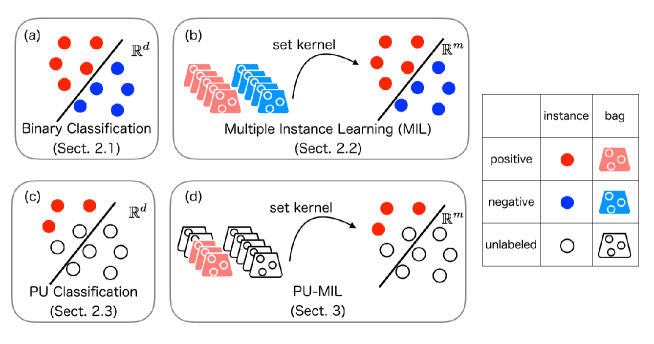
Figure 1: A schematic of problems. In this work, we consider (d) multiple instance learning from positive and unlabeled bags (PU-MIL).

2.1 Ordinary Binary Classification

Let $\bm{x}\in\mathbb{R}^{d}$ be a $d$-dimensional feature vector and $y\in\{+1,-1\}$ be its corresponding class label. In the ordinary binary classification problem, we construct a binary classifier

$$f(\bm{x}) =\mathrm{sign}(g(\bm{x}))\in\{+1,-1\},$$

$$g :\mathbb{R}^{d}\to\mathbb{R},$$ (1)

from an i.i.d. training dataset $\mathcal{D}=\{(\bm{x}_{i},y_{i})\}_{i=1}^{N}$, where $N$ is the number of training samples. Here we use a linear-in-parameter model for $g$:

$$g(\bm{x})=\bm{\alpha}^{\top}\bm{\phi}(\bm{x})+\beta,$$

where $\top$ denotes the transpose, $\bm{\alpha}\in\mathbb{R}^{m}$ is an $m$-dimensional parameter vector, $\beta\in\mathbb{R}$ is a bias parameter, and $\bm{\phi}:\mathbb{R}^{d}\to\mathbb{R}^{m}$ is a vector of basis functions. The support vector machine (SVM) [29] is one of the most standard methods for training a binary classifier. The optimization problem of SVM is given as follows:

$$\min_{\bm{\alpha}\in\mathbb{R}^{m},\beta\in\mathbb{R}}\quad \frac{1}{2}||\bm{\alpha}||^{2}+C\sum_{i=1}^{N}\max\left\{0,1-y_{i}\left(\bm{\alpha}^{\top}\bm{\phi}(\bm{x}_{i})+\beta\right)\right\},$$ (2)

where $C>0$ is a penalty parameter. This problem can be reformulated as a quadratic program (QP), which can be solved efficiently.

2.2 Multiple Instance Learning

We formulate the problem of multiple instance learning (MIL) and review an existing method.

2.2.1 Formulation

Hereafter $\mathcal{P}(A)$ denotes the power set of $A$. Let $X=\{\bm{x}_{i}|\bm{x}_{i}\in\mathbb{R}^{d}\}_{i=1}^{n}\in\mathcal{P}(\mathbb{R}^{d})\setminus\emptyset$ be a bag containing $n$ instances whose dimensions are $d$, and $Y\in\{+1,-1\}$ be a bag label corresponding to $X$. The problem is to construct a binary classifier:

$$f(X) =\mathrm{sign}(g(X))\in\{+1,-1\},$$

$$g :\mathcal{P}(\mathbb{R}^{d})\setminus\emptyset\to\mathbb{R},$$ (3)

from an i.i.d. fully-labeled training dataset $\mathcal{D}=\{(X_{b},Y_{b})\}_{b=1}^{N}$, where $N$ denotes the number of bags in $\mathcal{D}$.

2.2.2 Multiple Instance Kernels

Gärtner et al. [20] proposed set kernels (multiple instance kernels), which map bags (sets of instances) to a feature space. A type of the set kernels, called the statistic kernel $\widetilde{k}$, is defined as follows:

$$\widetilde{k}(X,X^{\prime}):=k(\bm{s}(X),\bm{s}(X^{\prime})),$$

where $k$ is an arbitrary kernel function such as the Gaussian kernel, and $\bm{s}$ is called a statistic. For example, the following minimax statistics is a typical choice:

$$\bm{s}_{\mathrm{minimax}}(X) :=\left[\min_{\bm{x}\in X}x^{(1)},\;\ldots,\;\min_{\bm{x}\in X}x^{(d)},\;\max_{\bm{x}\in X}x^{(1)},\;\ldots,\;\max_{\bm{x}\in X}x^{(d)}\right]^{\top},$$ (4)

where $x^{(i)}$ is the $i$-th element of an instance $\bm{x}$ in the bag $X$. Gärtner et al. [20] experimentally demonstrated that the statistic kernel with the minimax statistics (4) for $\bm{s}$ and the polynomial kernel for $k$ shows good performance:

$$\widetilde{k}_{\mathrm{minimax}}(X,X^{\prime}) :=(\bm{s}_{\mathrm{minimax}}(X)^{\top}\bm{s}_{\mathrm{minimax}}(X^{\prime})+1)^{\rho},$$ (5)

where $\rho$ is a positive integer. The statistic kernel (5) is referred to as the minimax kernel. We can then construct the following set kernel classifier $g$:

$$g(X) =\bm{\alpha}^{\top}\bm{\phi}(X)+\beta,$$ (6)

$$\bm{\phi}(X) =\left[\begin{array}[]{c}\widetilde{k}_{\mathrm{minimax}}(X,C_{1})\\ \vdots\\ \widetilde{k}_{\mathrm{minimax}}(X,C_{M})\end{array}\right],$$ (10)

where $C_{1},\ldots,C_{M}$ are kernel centers and $M$ is the number of kernel centers. We can obtain the MIL classifier by using SVM (2) to train the classifier (6).

2.3 Learning from Positive and Unlabeled Data

We formulate a binary classification problem from positive and unlabeled instances and review existing methods.

2.3.1 Formulation

We assume that positive samples $\{\bm{x}_{i}^{\mathrm{P}}\}_{i=1}^{N_{\mathrm{P}}}$ and unlabeled samples $\{\bm{x}_{i}^{\mathrm{U}}\}_{i=1}^{N_{\mathrm{U}}}$ are generated as follows:

$$\{\bm{x}_{i}^{\mathrm{P}}\}_{i=1}^{N_{\mathrm{P}}}\stackrel{{\scriptstyle\mathrm{i.i.d.}}}{{\sim}} \;p_{+}(\bm{x}):=p(\bm{x}|y=+1),$$

$$\{\bm{x}_{i}^{\mathrm{U}}\}_{i=1}^{N_{\mathrm{U}}}\stackrel{{\scriptstyle\mathrm{i.i.d.}}}{{\sim}} \;p(\bm{x}):=\pi p(\bm{x}|y=+1)+(1-\pi)p(\bm{x}|y=-1)$$

$$\hskip 24.0pt=\pi p_{+}(\bm{x})+(1-\pi)p_{-}(\bm{x}),$$ (11)

where $\pi:=p(y=+1)$ is called the class prior. Our objective is to construct the binary classifier (1) only from positive and unlabeled samples.

2.3.2 Learning Instance-Level Classifiers from Positive and Unlabeled Data

du Plessis et al. [28, 23] proposed methods based on empirical risk minimization to learn only from positive and unlabeled samples. In the ordinary binary classification setting, an optimal classifier $g^{*}$ minimizes the following misclassification rate:

$$R_{0\mbox{-}1}(g)=\pi\mathbb{E}_{{\mathrm{P}}}\left[{\ell_{0\mbox{-}1}(g(\bm{x}))}\right]+(1-\pi)\mathbb{E}_{{\mathrm{N}}}\left[{\ell_{0\mbox{-}1}(-g(\bm{x}))}\right],$$ (12)

where $\mathbb{E}_{{\mathrm{P}}}\left[{\cdot}\right]$ and $\mathbb{E}_{{\mathrm{N}}}\left[{\cdot}\right]$ denote the expectations over $p_{+}(\bm{x})$ and $p_{-}(\bm{x})$ respectively and $\ell_{0\mbox{-}1}$ denotes the zero-one loss:

$$\ell_{0\mbox{-}1}(z)=\begin{cases}0&\mbox{if $z\geq 0$,}\\ 1&\mbox{otherwise.}\end{cases}$$

In practice, the misclassification rate (12) is difficult to optimize because the subgradient of $\ell_{0\mbox{-}1}$ is always $0$ except at $z=0$. For this reason, we usually use a surrogate loss function. Then the risk function $R$ with the surrogate loss function $\ell$ is written as

$$R(g):=\pi\mathbb{E}_{{\mathrm{P}}}\left[{\ell(g(\bm{x}))}\right]+(1-\pi)\mathbb{E}_{{\mathrm{N}}}\left[{\ell(-g(\bm{x}))}\right].$$ (13)

Since negative samples are not available in the PU classification setup, let us consider expressing the risk (13) without $\mathbb{E}_{{\mathrm{N}}}\left[{\cdot}\right]$. By the definition of the unlabeled sample distribution (11), the following equation holds:

$$(1-\pi)\mathbb{E}_{{\mathrm{N}}}\left[{\ell(-g(\bm{x}))}\right]=\mathbb{E}_{{\mathrm{U}}}\left[{\ell(-g(\bm{x}))}\right]-\pi\mathbb{E}_{{\mathrm{P}}}\left[{\ell(-g(\bm{x}))}\right].$$

Substituting this into the risk (13), we obtain

$$R(g)=\pi\mathbb{E}_{{\mathrm{P}}}\left[{\ell(g(\bm{x}))-\ell(-g(\bm{x}))}\right]+\mathbb{E}_{{\mathrm{U}}}\left[{\ell(-g(\bm{x}))}\right],$$ (14)

where $\mathbb{E}_{{\mathrm{U}}}\left[{\cdot}\right]$ denotes the expectation over $p(\bm{x})$. If the surrogate loss function $\ell$ satisfies

$$\ell(z)-\ell(-z)=-z,$$ (15)

the risk (14) can be written as

$$R(g)=\pi\mathbb{E}_{{\mathrm{P}}}\left[{-g(\bm{x})}\right]+\mathbb{E}_{{\mathrm{U}}}\left[{\ell(-g(\bm{x}))}\right].$$ (16)

The risk (16) is convex if the surrogate loss function $\ell$ is convex. Convex loss functions such as the squared loss $\ell_{\mathrm{S}}$, the logistic loss $\ell_{\mathrm{LL}}$, and the double hinge loss $\ell_{\mathrm{DH}}$ satisfy the condition (15):

$$\ell_{\mathrm{S}}(z) =\frac{1}{4}(z-1)^{2},$$

$$\ell_{\mathrm{LL}}(z) =\log(1+\exp(-z)),$$

$$\ell_{\mathrm{DH}}(z) =\max\left(-z,\max\left(0,\frac{1-z}{2}\right)\right).$$ (17)

We use the risk (16) to obtain a convex formulation of PU-MIL in Sect. 3.

3 Positive and Unlabeled Set Kernel Classifier

In this section, we propose a convex method for PU-MIL, named the PU-SKC (positive and unlabeled set kernel classifier).

3.1 Multiple Instance Learning from Positive and Unlabeled Bags

We formulate the problem of multiple instance learning from positive and unlabeled bags (PU-MIL). The purpose of PU-MIL is to construct the bag-level classifier (3) from a positively labeled training dataset $\mathcal{D}_{\mathrm{P}}=\{(X_{b}^{\mathrm{P}},Y_{b}=+1)\}_{b=1}^{N_{\mathrm{P}}}$ and an unlabeled training dataset $\mathcal{D}_{\mathrm{U}}=\{X_{b^{\prime}}^{\mathrm{U}}\}_{{b^{\prime}}=1}^{N_{\mathrm{U}}}$, where $N_{\mathrm{P}}$ and $N_{\mathrm{U}}$ denote the number of positive bags in $\mathcal{D}_{\mathrm{P}}$ and the number of unlabeled bags in $\mathcal{D}_{\mathrm{U}}$, respectively. We assume that $X_{1}^{\mathrm{P}},\dots,X_{N_{\mathrm{P}}}^{\mathrm{P}}\stackrel{{\scriptstyle\mathrm{i.i.d.}}}{{\sim}}p(X|Y=+1)$ and $X_{1}^{\mathrm{U}},\dots,X_{N_{\mathrm{U}}}^{\mathrm{U}}\stackrel{{\scriptstyle\mathrm{i.i.d.}}}{{\sim}}p(X)$.

3.2 Formulation

As we mentioned in Sect. 2.3, du Plessis et al. [28, 23] formulated the PU classification problem in the empirical risk minimization framework. If we use a loss function $l(z)$ such that $l(z)-l(-z)=-z$, we have the following objective function:

$$J(g)=\pi\mathbb{E}_{{\mathrm{P}}}\left[{-g(X)}\right]+\mathbb{E}_{{\mathrm{U}}}\left[{\ell(-g(X))}\right].$$ (18)

Here we use a linear-in-parameter model with the set kernel function as a classifier:

$$g(X)=\bm{\alpha}^{\top}\bm{\phi}(X)+\beta,$$ (19)

where $\bm{\phi}$ is a vector of basis functions:

$$\bm{\phi}(X)=\left[\begin{array}[]{c}\widetilde{k}_{\mathrm{minimax}}(X,X^{\mathrm{P}}_{1})\\ \vdots\\ \widetilde{k}_{\mathrm{minimax}}(X,X^{\mathrm{P}}_{N_{\mathrm{P}}})\\ \widetilde{k}_{\mathrm{minimax}}(X,X^{\mathrm{U}}_{1})\\ \vdots\\ \widetilde{k}_{\mathrm{minimax}}(X,X^{\mathrm{U}}_{N_{\mathrm{U}}})\end{array}\right].$$ (26)

As with the standard binary classification, we predict a given bag as positive if $g(X)\geq 0$, and as negative if $g(X)<0$.

The risk (18) together with the bag-level classifier (19) and the $l_{2}$ regularizer induces the following objective function to be minimized:

$$\widehat{J}(\bm{\alpha},b) =\pi\cdot\frac{1}{N_{\mathrm{P}}}\sum_{b=1}^{N_{\mathrm{P}}}\left(-\bm{\alpha}^{\top}\bm{\phi}(X^{\mathrm{P}}_{b})-\beta\right)$$

$$+\frac{1}{N_{\mathrm{U}}}\sum_{{b^{\prime}}=1}^{N_{\mathrm{U}}}\ell_{\mathrm{DH}}\left(-\bm{\alpha}^{\top}\bm{\phi}(X^{\mathrm{U}}_{b^{\prime}})-\beta\right)+\frac{\lambda}{2}\bm{\alpha}^{\top}\bm{\alpha},$$ (27)

where $\lambda\geq 0$ is the regularization parameter. Here we use the double hinge loss $\ell_{\mathrm{DH}}$ (17) because du Plessis et al. [23] reported that it achieved the best performance in the ordinary PU classification setting. Note that $\pi$ is the bag-level class prior, i.e., $\pi=p(Y=+1)$, which must be estimated from the training data. We explain how to estimate it in Sect. 3.3.

The problem of minimizing (27) can be rewritten in the form of a quadratic program by using slack variables $\bm{\xi}$ as

$$\min_{\bm{\alpha},\beta,\bm{\xi}}\quad -\frac{\pi}{N_{\mathrm{P}}}\bm{1}^{\top}\Phi_{\mathrm{P}}\bm{\alpha}-\pi\beta+\frac{1}{N_{\mathrm{U}}}\bm{1}^{\top}\bm{\xi}+\frac{\lambda}{2}\bm{\alpha}^{\top}\bm{\alpha}$$ (28)

s.t. $$\bm{\xi}\geq\bm{0},$$

$$\bm{\xi}\geq\frac{1}{2}\bm{1}+\frac{1}{2}\Phi_{\mathrm{U}}\bm{\alpha}+\frac{1}{2}\beta\bm{1},$$

$$\bm{\xi}\geq\Phi_{\mathrm{U}}\bm{\alpha}+\beta\bm{1},$$

where $\geq$ for vectors denotes the element-wise inequality, and $\bm{0}$, $\bm{1}$ denote the all-zero and all-one vectors, respectively. Matrices $\Phi_{\mathrm{P}}$ and $\Phi_{\mathrm{U}}$ are defined as follows:

$$\Phi_{\mathrm{P}}=\left[\begin{array}[]{c}\bm{\phi}^{\top}(X^{\mathrm{P}}_{1})\\ \vdots\\ \bm{\phi}^{\top}(X^{\mathrm{P}}_{N_{\mathrm{P}}})\end{array}\right],\quad\Phi_{\mathrm{U}}=\left[\begin{array}[]{c}\bm{\phi}^{\top}(X^{\mathrm{U}}_{1})\\ \vdots\\ \bm{\phi}^{\top}(X^{\mathrm{U}}_{N_{\mathrm{U}}})\end{array}\right].$$

Note that our proposed method is independent of kernel choices. Other set kernels, such as the conformal kernels [31] and affinity propagation clustering-based feature representation [32], can also be used instead of the polynomial minimax kernel, depending on domain-specific knowledge.

3.3 Bag-Level Class Prior Estimation

A bag-level class prior estimation algorithm can be obtained by a simple extension of the instance-level version explained in A. The difference is basis functions used for estimating the class prior. We use the polynomial minimax kernel (5) to obtain the bag-level basis functions (26). Then the bag-level class prior $\pi$ can be estimated similarly:

$$\pi=\left[2\widehat{\bm{h}}^{\top}\widehat{G}^{-1}\widehat{\bm{h}}-\widehat{\bm{h}}^{\top}\widehat{G}^{-1}\widehat{H}\widehat{G}^{-1}\widehat{\bm{h}}\right]^{-1},$$

where

$$\widehat{H}=\frac{1}{N_{\mathrm{P}}}\sum_{b=1}^{N_{\mathrm{P}}}\bm{\phi}(X_{b}^{\mathrm{P}})\bm{\phi}(X_{b}^{\mathrm{P}})^{\top},\quad\widehat{\bm{h}}=\frac{1}{N_{\mathrm{U}}}\sum_{b^{\prime}=1}^{N_{\mathrm{U}}}\bm{\phi}(X_{b^{\prime}}^{\mathrm{U}}),\quad\widehat{G}=\widehat{H}+\eta I,$$

and $\eta>0$ is another regularization parameter. The detailed derivation is described in A.

3.4 Remarks: Instance-Level PU-MIL

PU-SKC is a bag-level method, namely, classifying bags directly (Eq. (19)) instead of aggregating instance-level classification results. On the other hand, we can also consider an instance-level method to solve PU-MIL.

Assume that instances in negative bags are drawn from the instance-level negative conditional distribution, i.e.,

$$\bm{x}\stackrel{{\scriptstyle\mathrm{i.i.d.}}}{{\sim}}p(\bm{x}|y=-1)\quad\text{for every $\bm{x}\in X^{\mathrm{N}}$},$$ (29)

and instances in positive bags are drawn from the instance-level marginal distribution, i.e.,

$$\bm{x}\stackrel{{\scriptstyle\mathrm{i.i.d.}}}{{\sim}}p(\bm{x})=\theta p(\bm{x}|y=+1)+(1-\theta)p(\bm{x}|y=-1)\quad\text{for every $\bm{x}\in X^{\mathrm{P}}$},$$ (30)

where $\theta:=p(y=+1)$ is the instance-level class prior. Since we assume the bag-level class prior $p(Y=+1)=\pi$, instances in unlabeled bags are drawn from the following distribution, i.e.,

$$\bm{x}\stackrel{{\scriptstyle\mathrm{i.i.d.}}}{{\sim}}p^{\prime}(\bm{x}) =\pi p(\bm{x})+(1-\pi)p(\bm{x}|y=-1)$$

$$=\pi\theta p(\bm{x}|y=+1)+(1-\pi\theta)p(\bm{x}|y=-1)\quad\text{for every $\bm{x}\in X^{\mathrm{U}}$}.$$ (31)

From the instance-level perspective, both positive and unlabeled bags are unlabeled datasets, but the class proportions are different ($\theta$ for Eq. (30) and $\pi\theta$ for Eq. (31)). In fact, an (instance-level) binary classifier can be obtained from two distinct datasets with different class proportions [33].

Assume that the test class priors are equal $q(y=+1)=q(y=-1)=1/2$ and the test conditional density $q(\bm{x}|y)$ is equal to $p(\bm{x}|y)$. We begin with the difference of the class posteriors:

$$q(y=+1|\bm{x})-q(y=-1|\bm{x}) =\frac{q(\bm{x}|y=+1)q(y=+1)}{q(\bm{x})}-\frac{q(\bm{x}|y=-1)q(y=-1)}{q(\bm{x})}$$

$$=\frac{p(\bm{x}|y=+1)\frac{1}{2}}{q(\bm{x})}-\frac{p(\bm{x}|y=-1)\frac{1}{2}}{q(\bm{x})}$$

$$=\frac{1}{2q(\bm{x})}(p(\bm{x}|y=+1)-p(\bm{x}|y=-1)).$$

Since $2q(\bm{x})$ is always positive, the classification criterion on the test distribution becomes

$$d(\bm{x})=\mathrm{sign}[p(\bm{x}|y=+1)-p(\bm{x}|y=-1)].$$

On the other hand,

$$p(\bm{x})-p^{\prime}(\bm{x}) =(\theta-\pi\theta)p(\bm{x}|y=+1)-((1-\theta)-(1-\pi\theta))p(\bm{x}|y=-1)$$

$$=\theta(1-\pi)[p(\bm{x}|y=+1)-p(\bm{x}|y=-1)].$$

Since $\theta(1-\pi)>0$, the classification criterion becomes

$$d(\bm{x})=\mathrm{sign}[p(\bm{x})-p^{\prime}(\bm{x})].$$ (32)

The point is, in order to obtain an instance-level classifier, all we have to do is to estimate the density difference $p(\bm{x})-p^{\prime}(\bm{x})$. To this end, a method called least-squares density difference (LSDD) estimation has been proposed [34]. A more advanced method to estimate the sign of the density difference $\mathrm{sign}[p(\bm{x})-p^{\prime}(\bm{x})]$ directly has also been proposed [33], which is called direct sign density difference (DSDD) estimation. These estimators are also compared as baselines in experiments.

The instance-level approach is useful when our goal is to determine all instance-level labels. Otherwise, the bag-level approach is suitable because it is a direct approach to determine only bag-level labels, which is referred to as Vapnik’s principle [35]:

When solving a problem of interest, one should not solve a more general problem as an intermediate step.

Here, knowing instance-level labels allows us to identify bag-level labels, but not vice versa. In this sense, obtaining an instance-level classifier is regarded as solving an intermediate/general problem when our goal is to predict labels for bags.

4 Analysis of Generalization Error Bounds

In this section, we show an upper bound of the generalization error (evaluated on a fixed classifier) for our proposed method. Let $\mathscr{X}:=\mathcal{P}(\mathbb{R}^{d})\setminus\emptyset$ be the bag-level domain set and

$$\mathcal{G}:=\left\{g(X)=\bm{\alpha}^{\top}\bm{\phi}(X)\;\middle|\;\|\bm{\alpha}\|\leq C_{\bm{\alpha}},\sup_{X\in\mathscr{X}}\|\bm{\phi}(X)\|\leq C_{\bm{\phi}}\right\}$$ (33)

be a given function class, where $\bm{\phi}$ is a vector of basis functions defined in Eq. (26). Note that $\mathcal{G}$ includes the classifier (19) as a special case. Throughout this section, let $\ell:\mathbb{R}\rightarrow\mathbb{R}_{+}$ be the double hinge loss (17), which is used in our experiments. We denote the expected risk of a bag-level classifier $g:\mathscr{X}\rightarrow\mathbb{R}$ with respect to $\ell$ as

$$\mathcal{R}(g) :=\mathbb{E}_{p(X,Y)}[\ell(Yg(X))]$$

$$=\pi^{*}\mathbb{E}_{p(X|Y=+1)}[-g(X)]+\mathbb{E}_{p(X)}[\ell(-g(X))],$$

and the corresponding empirical risk as

$$\widehat{\mathcal{R}}(g):=-\frac{\pi^{*}}{N_{\mathrm{P}}}\sum_{b=1}^{N_{\mathrm{P}}}g(X_{b}^{\mathrm{P}})+\frac{1}{N_{\mathrm{U}}}\sum_{b^{\prime}=1}^{N_{\mathrm{U}}}\ell(-g(X_{b^{\prime}}^{\mathrm{U}})),$$

where $\pi^{*}:=p(Y=+1)$ is the true class prior of the positive class.

Theorem 1.

For a fixed $g\in\mathcal{G}$, and for any $\delta\in(0,1)$, with probability at least $1-\delta$,

$$\mathcal{R}(g)-\widehat{\mathcal{R}}(g)\leq C_{\mathcal{G},\delta}\left(\frac{2\pi^{*}}{\sqrt{N_{\mathrm{P}}}}+\frac{1}{\sqrt{N_{\mathrm{U}}}}\right),$$ (34)

where $C_{\mathcal{G},\delta}>0$ is a constant depending jointly on $\mathcal{G}$ and $\delta$.

The proof is in C. This theorem shows that the generalization error decreases with order $1/\sqrt{N_{\mathrm{P}}}$ and $1/\sqrt{N_{\mathrm{U}}}$. Thus, increasing the number of positive bags and the number of unlabeled bags both contributes to reducing the error. Note that this order is optimal in a parametric setup [30]. Furthermore, we can see from Eq. (34) that the true class prior $\pi^{*}$ and $N_{\mathrm{P}}$ are related in the generalization error bound, while $\pi^{*}$ and $N_{\mathrm{U}}$ are not. We will further investigate this issue through experiments in Section 5.

5 Experiments

In this section, we experimentally compare the proposed method with the baselines (Sect. 3.4), and an existing method (see B) and give answers to the following research questions.

 
Q1: Does the proposed method outperform the baseline and existing methods regardless of the true class prior?
Q2: Is the proposed method computationally efficient?

5.1 Datasets

We used standard MIL datasets: Musk and Corel. The details of these benchmark datasets are shown in Table 2.

Table 2: Details of datasets: The last two rows indicate the numbers of instances per bag, which are the average with standard deviation.

Number of	Musk1	Musk2	Elephant	Fox	Tiger
features	166	166	230	230	230
positive bags	47	39	100	100	100
negative bags	45	63	100	100	100
positive instances	2.3 (2.6)	10.0 (26.1)	3.8 (4.2)	3.2 (3.6)	2.7 (3.1)
negative instances	2.9 (6.9)	54.7 (176.0)	3.2 (3.6)	3.4 (3.8)	3.4 (3.8)

Since these datasets are too small to evaluate PU methods, we augmented them to increase the number of bags. Specifically, bags chosen randomly from the original datasets were duplicated and then Gaussian noise with mean zero and variance $0.01$ was added to each dimension. In this way, we increased the number of samples in the Musk datasets (Musk1 and Musk2) 10 times and the Corel datasets (Elephant, Fox, and Tiger) 5 times. After this augmentation process, we generated a training set (including labeled positive bags and unlabeled bags) and a test set. This generation process is described in Algorithm 1 (we set $L=20,U=180$, and $T=200$).

Remark: This dataset processing is needed. The reasons are as follows.

1. We assume that the training distribution and test distribution are same, which means that the class priors are same, too. Thus Algorithm 1 is needed to maintain the class priors to be same among both (unlabeled) training and test datasets.

2. If Algorithm 1 is applied, it is hard to obtain an enough number of negative bag samples under extremely low class priors, while maintaining the class priors to be same. Thus the augmentation process is needed.

Algorithm 1 Generation of Training / Test Sets for Benchmark MIL Datasets

1:$\mathcal{D}_{\mathrm{P}}$: original positive bags, $\mathcal{D}_{\mathrm{N}}$: original negative bags, $\pi$: true bag-level class prior, $L$: #{labeled positive bags}, $U$: #{unlabeled bags}, $T$: #{test bags}

2:$\mathcal{D}_{\mathrm{L}}\subset\mathcal{D}_{\mathrm{P}}$ $\triangleright$ $\lvert\mathcal{D}_{\mathrm{L}}\rvert=L$

3:$\mathcal{D}_{\mathrm{P}}:=\mathcal{D}_{\mathrm{P}}\setminus\mathcal{D}_{\mathrm{L}}$

4:$N_{\mathrm{U}}^{\mathrm{P}}\sim B(U+T,\pi)$

5:$N_{\mathrm{U}}^{\mathrm{N}}:=U+T-N_{\mathrm{U}}^{\mathrm{P}}$

6:$\mathcal{D}_{\mathrm{U}}:=\mathcal{D}_{\mathrm{P}}^{\prime}(\subset\mathcal{D}_{\mathrm{P}})\cup\mathcal{D}_{\mathrm{N}}^{\prime}(\subset\mathcal{D}_{\mathrm{N}})$ $\triangleright$ $\lvert\mathcal{D}_{\mathrm{P}}^{\prime}\rvert=N_{\mathrm{U}}^{\mathrm{P}},\lvert\mathcal{D}_{\mathrm{N}}^{\prime}\rvert=N_{\mathrm{U}}^{\mathrm{N}}$

7:$\mathcal{D}_{\mathrm{U}}^{\prime}\subset\mathcal{D}_{\mathrm{U}}$ $\triangleright$ $\lvert\mathcal{D}_{\mathrm{U}}^{\prime}\rvert=T$

8:$\mathcal{D}_{\mathrm{U}}:=\mathcal{D}_{\mathrm{U}}\setminus\mathcal{D}_{\mathrm{U}}^{\prime}$

9:$\mathcal{D}_{\mathrm{L}}\cup\mathcal{D}_{\mathrm{U}}$: training set, $\mathcal{D}_{\mathrm{U}}^{\prime}$: test set

5.2 Methods

We compared the following methods:

• Positive-Unlabeled Set Kernel Classifier (PU-SKC, the proposed method): Hyperparameters (the degree parameter $\rho$ in the polynomial kernel (5) and the regularization parameter $\lambda$ in the objective function (27)) were selected via 5-fold cross-validation from $\rho\in[1,2,3]$ and $\lambda\in[10^{0},10^{-3},10^{-6}]$. Values minimizing the PU risk (16) with the zero-one loss were chosen to be optimal.

• Least-Squares Density Difference (LSDD): Estimate the density difference $p(\bm{x})-p^{\prime}(\bm{x})$ to obtain (32) using the least-squares method [34]. The bag classifier can be obtained as $g(X)=\max_{\bm{x}\in X}d(\bm{x})$. Hyperparameters (the width of the Gaussian kernel $s$ and the regularization parameter $\lambda$) were selected via 5-fold cross-validation from $s\in[10^{-2},10^{-4},10^{-6}]$ and $\lambda\in[10^{0},10^{-3},10^{-6}]$.

• Direct Sign of Density Difference (DSDD): Estimate the sign of the density difference (32) directly [33]. The bag classifier can be obtained in the same way as LSDD. Hyperparameters (the width of the Gaussian kernel $s$ and the regularization parameter $\lambda$) were selected via 5-fold cross-validation from $s\in[10^{-2},10^{-4},10^{-6}]$ and $\lambda\in[10^{0},10^{-3},10^{-6}]$.

• puMIL: An SVM-based approach [27]. The detail is described in B.

5.3 Results

Here we show the experimental results and give answers to the research questions.

5.3.1 Classification Performances

Table 3: Each result is the average with standard deviation of the classification accuracy over 20 trials. Bold faces represent the best methods under each setting (tested by the one-sided 5% t-test).

dataset	$\pi$	PU-SKC	LSDD [34]	DSDD [33]	puMIL [27]
Musk1	0.1	0.865 (0.046)	0.928 (0.029)	0.931 (0.026)	0.757 (0.065)
	0.2	0.844 (0.038)	0.707 (0.289)	0.876 (0.037)	0.733 (0.070)
	0.3	0.818 (0.041)	0.622 (0.208)	0.778 (0.045)	0.717 (0.063)
	0.4	0.776 (0.057)	0.618 (0.148)	0.708 (0.041)	0.699 (0.050)
	0.5	0.763 (0.050)	0.553 (0.072)	0.597 (0.047)	0.665 (0.081)
	0.6	0.735 (0.055)	0.522 (0.068)	0.505 (0.051)	0.649 (0.069)
	0.7	0.737 (0.044)	0.538 (0.161)	0.392 (0.061)	0.606 (0.075)
Musk2	0.1	0.810 (0.060)	0.702 (0.303)	0.840 (0.040)	0.688 (0.098)
	0.2	0.802 (0.053)	0.691 (0.239)	0.789 (0.036)	0.730 (0.063)
	0.3	0.801 (0.051)	0.621 (0.173)	0.720 (0.050)	0.732 (0.073)
	0.4	0.724 (0.063)	0.590 (0.111)	0.621 (0.048)	0.704 (0.068)
	0.5	0.742 (0.050)	0.522 (0.054)	0.537 (0.055)	0.654 (0.092)
	0.6	0.706 (0.059)	0.499 (0.086)	0.466 (0.053)	0.637 (0.086)
	0.7	0.726 (0.055)	0.508 (0.159)	0.364 (0.063)	0.599 (0.072)
Elephant	0.1	0.845 (0.044)	0.734 (0.153)	0.747 (0.041)	0.722 (0.084)
	0.2	0.783 (0.062)	0.671 (0.166)	0.715 (0.039)	0.686 (0.075)
	0.3	0.746 (0.062)	0.652 (0.092)	0.685 (0.038)	0.698 (0.072)
	0.4	0.701 (0.050)	0.573 (0.088)	0.608 (0.039)	0.642 (0.051)
	0.5	0.607 (0.058)	0.552 (0.052)	0.575 (0.050)	0.667 (0.070)
	0.6	0.528 (0.087)	0.520 (0.062)	0.503 (0.031)	0.614 (0.063)
	0.7	0.421 (0.059)	0.602 (0.141)	0.453 (0.037)	0.597 (0.066)
Fox	0.1	0.840 (0.053)	0.634 (0.181)	0.717 (0.037)	0.561 (0.062)
	0.2	0.754 (0.048)	0.689 (0.042)	0.669 (0.041)	0.575 (0.058)
	0.3	0.689 (0.054)	0.576 (0.130)	0.615 (0.045)	0.544 (0.045)
	0.4	0.613 (0.061)	0.542 (0.097)	0.588 (0.041)	0.552 (0.053)
	0.5	0.538 (0.042)	0.527 (0.046)	0.545 (0.042)	0.547 (0.074)
	0.6	0.468 (0.057)	0.538 (0.071)	0.464 (0.053)	0.550 (0.055)
	0.7	0.430 (0.055)	0.559 (0.151)	0.430 (0.046)	0.536 (0.075)
Tiger	0.1	0.839 (0.044)	0.689 (0.136)	0.730 (0.047)	0.706 (0.073)
	0.2	0.783 (0.035)	0.695 (0.032)	0.707 (0.031)	0.680 (0.070)
	0.3	0.729 (0.043)	0.636 (0.047)	0.651 (0.052)	0.659 (0.056)
	0.4	0.672 (0.043)	0.596 (0.042)	0.606 (0.036)	0.668 (0.048)
	0.5	0.584 (0.043)	0.566 (0.044)	0.540 (0.046)	0.609 (0.070)
	0.6	0.508 (0.048)	0.530 (0.066)	0.523 (0.032)	0.608 (0.080)
	0.7	0.410 (0.059)	0.490 (0.080)	0.463 (0.034)	0.585 (0.086)

Table 3 shows averages with standard deviations of the classification accuracy over $20$ trials under each class prior. Bold faces represent the best methods under each class prior. This was tested by the one-sided t-test with 5% significance level (first the best method was chosen, then other methods were checked whether they are comparable or not by the one-sided t-test). As it can be seen from Table 3, PU-SKC outperforms the existing method puMIL [27] under various class priors. Note that the true class prior in Table 3 means the predefined value for dataset generation (see Algorithm 1), not an estimated class prior during the learning process (see Sect. 3.3).

Overall, the performance of the proposed method decreases as the true class prior becomes higher. This can be confirmed from Eq. (34): since $2\pi^{*}/\sqrt{N_{\mathrm{P}}}$ dominates the upper bound given sufficiently large $N_{\mathrm{U}}$, more positive bags are needed to achieve accurate classification performance compared with a small class prior case. In practice, we could address this issue by collecting more positive bags. Figure 2 shows classification performances under different number of positive bags. Classification performances are improved as the number of positive bags increases.

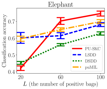
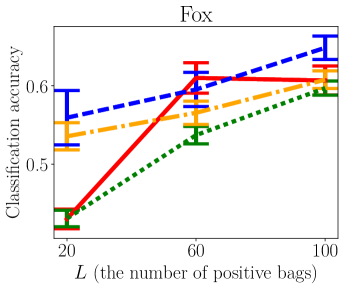
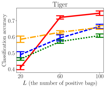
Figure 2: Classification performances of each dataset under different number of positive bags. The number of unlabeled bags are fixed to 180. The true class priors are set to $0.7$ among all settings.

A1: The proposed method tends to outperform the baseline and existing methods under various class priors.

5.3.2 Computation Time

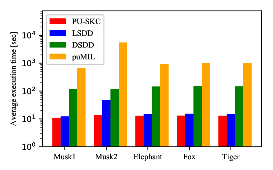
Figure 3: Average execution time: each result is the average execution time of 20 trials under bag-level class prior $\pi=0.1$. PU-SKC is executed on the given hyperparameter.

Next, we compared the execution time between the proposed method and the baseline and existing methods. The result is shown in Figure 3. This result shows that PU-SKC is much more computationally efficient than the baseline and existing methods. Note that the execution time in other class prior values ($\pi=0.2,0.3,\dots,0.7$) is almost the same as the one shown in Figure 3 because both the class prior estimation algorithm shown in Sec 3.3 and the PU-SKC optimization problem (28) are non-iterative methods and their computation complexities do not depend on the value of $\pi$ or its estimated value.

A2: The proposed method is much more computationally efficient than the baseline and existing methods.

6 Conclusion

In this work, we considered a multiple instance learning problem when only positive bags and unlabeled bags are available, which does not require all training bags to be labeled. We proposed a convex method, PU-SKC, to solve PU multiple instance classification. This method is based on the convex formulation of PU classification [23] and the set kernel [20]. PU-SKC performed better than the existing PU multiple instance classification method [27] on benchmark MIL datasets. Furthermore, we confirmed that the proposed method was much more computationally efficient than the baseline and existing methods through the experiment.

Reference

Appendix A Instance-Level Class Prior Estimation

In the research by du Plessis and Sugiyama [36], a class prior estimation method from positive and unlabeled data by partial matching was proposed. This method estimates the class prior $\pi$ by minimizing the Pearson (PE) divergence from positive data distribution $\pi p(\bm{x}|y=1)$ to unlabeled data distribution $p(\bm{x})$:

$$\pi^{*} =\mathop{\rm arg~{}min}\limits_{\pi}\textsf{PE}[\pi p(\bm{x}|y=1)|p(\bm{x})]$$

$$=\mathop{\rm arg~{}min}\limits_{\pi}\frac{1}{2}\int\left(\frac{\pi p(\bm{x}|y=1)}{p(\bm{x})}-1\right)^{2}p(\bm{x})\mathrm{d}\bm{x}.$$

It is still possible to estimate $p(\bm{x}|y=1)$ from positive samples and $p(\bm{x})$ from unlabeled samples using, e.g., the kernel density estimation, but du Plessis and Sugiyama [36] empirically showed that such a naive approach often does not produce a good estimator of $\pi$. A better approach is to lower bound the PE divergence and directly maximize it:

$$\textsf{PE}[\pi p(\bm{x}|y=1)|p(\bm{x})]\geq \;\pi\int r(\bm{x})p(\bm{x}|y=1)\mathrm{d}\bm{x}$$

$$-\frac{1}{2}\int r(\bm{x})^{2}p(\bm{x})\mathrm{d}\bm{x}-\pi+\frac{1}{2},$$ (35)

where $r(\bm{x})$ is an arbitrary function. In practice, a linear-in-parameter model based on Gaussian kernel basis functions is used to estimate $r$:

$$\widehat{r}(\bm{x})=\bm{\alpha}^{\top}\bm{\phi}(\bm{x}).$$

Our goal is to find the tightest lower bound by maximizing the right-hand side of (35) at first with respect to $r$ and then minimize it with respect to $\pi$. The former maximization problem with the $l_{2}$ regularizer can be written as

$$\widehat{\bm{\alpha}} =\mathop{\rm arg~{}max}\limits_{\bm{\alpha}}\left[\pi\bm{\alpha}^{\top}\bm{h}-\frac{1}{2}\bm{\alpha}^{\top}H\bm{\alpha}-\pi+\frac{1}{2}-\frac{\lambda}{2}\bm{\alpha}^{\top}\bm{\alpha}\right]$$

$$=\mathop{\rm arg~{}max}\limits_{\bm{\alpha}}\left[\pi\bm{\alpha}^{\top}\bm{h}-\frac{1}{2}\bm{\alpha}^{\top}H\bm{\alpha}-\frac{\lambda}{2}\bm{\alpha}^{\top}\bm{\alpha}\right],$$ (36)

$$\mbox{where}\quad H =\int\bm{\phi}(\bm{x})\bm{\phi}(\bm{x})^{\top}p(\bm{x})\mathrm{d}\bm{x},\quad\bm{h}=\int\bm{\phi}(\bm{x})p(\bm{x}|y=1)\mathrm{d}\bm{x},$$

and $\lambda\geq 0$ denotes the regularization parameter. In practice, $H$ and $\bm{h}$ are estimated by the sample averages:

$$\widehat{H}=\frac{1}{N_{\mathrm{P}}}\sum_{i=1}^{N_{\mathrm{P}}}\bm{\phi}(\bm{x}^{\mathrm{P}}_{i})\bm{\phi}(\bm{x}^{\mathrm{P}}_{i})^{\top},\quad\widehat{\bm{h}}=\frac{1}{N_{\mathrm{U}}}\sum_{j=1}^{N_{\mathrm{U}}}\bm{\phi}(\bm{x}^{\mathrm{U}}_{j}).$$

Using these estimators, Eq. (36) can be reformulated as follows:

$$\widehat{\bm{\alpha}}=\mathop{\rm arg~{}max}\limits_{\bm{\alpha}}\left[\pi\bm{\alpha}^{\top}\widehat{\bm{h}}-\frac{1}{2}\bm{\alpha}^{\top}\widehat{H}\bm{\alpha}-\frac{\lambda}{2}\bm{\alpha}^{\top}\bm{\alpha}\right].$$

An analytical solution to the above problem can be obtained as follows:

$$\widehat{\bm{\alpha}}=\pi\widehat{G}^{-1}\widehat{\bm{h}},\quad\widehat{G}=\widehat{H}+\lambda I,$$

where $I$ denotes the identity matrix. This leads to the following PE divergence estimator:

$$\widehat{\textsf{PE}}=\pi^{2}\widehat{\bm{h}}^{\top}\widehat{G}^{-1}\widehat{\bm{h}}-\pi^{2}\frac{1}{2}\widehat{\bm{h}}^{\top}\widehat{G}^{-1}\widehat{H}\widehat{G}^{-1}\widehat{\bm{h}}-\pi+\frac{1}{2}.$$

Then the analytical minimizer of $\widehat{\textsf{PE}}$ can be obtained as

$$\widehat{\pi}=\left[2\widehat{\bm{h}}^{\top}\widehat{G}^{-1}\widehat{\bm{h}}-\widehat{\bm{h}}^{\top}\widehat{G}^{-1}\widehat{H}\widehat{G}^{-1}\widehat{\bm{h}}\right]^{-1}.$$

Appendix B Multiple Instance Learning from Positive and Unlabeled Bags

Wu et al. [27] proposed an instance-level method for the PU-MIL problem (called puMIL). As discussed in the previous work [15, 22], the key instance (the most positive instance) in each bag is important in MIL. This is also the case in PU-MIL, but the problem is that we cannot tell the labels of unlabeled bags. To address this issue, Wu et al. [27] introduced the bag confidence, which describes how much confident the given unlabeled bag is negative. Let $\nu_{b}\in[0,1]$ be the confidence of the $b$-th bag. Then the learning problem of an SVM classifier $g(X)=\bm{w}^{\top}\widetilde{\bm{x}}\quad(\widetilde{\bm{x}}\in X)$ under the given $\bm{\nu}$ is formulated as

$$\min_{\bm{w}\in\mathbb{R}^{d},\{\widetilde{\bm{x}}_{b}\}_{b=1}^{N_{\mathrm{P}}+N_{\mathrm{U}}}}\quad \frac{1}{2}||\bm{w}||^{2}+C\sum_{b=1}^{N_{\mathrm{P}}+N_{\mathrm{U}}}\max(0,1-\nu_{b}\widetilde{Y}_{b}\bm{w}^{\top}\widetilde{\bm{x}}_{b}),$$ (37)

where $\widetilde{Y}_{b}$ is the estimated bag label ($\widetilde{Y}_{b}=+1$ for a positive bag and $\widetilde{Y}_{b}=-1$ for a possibly negative bag coming from the set of unlabeled bags) and $\widetilde{\bm{x}}_{b}$ is the key instance in the bag $X_{b}$. $\nu_{b}$ weighs the contribution of $\widetilde{\bm{x}}_{b}$ according to its confidence. For positive bags, the confidence is simply set as $\nu_{b}=1$. The overall training method is summarized as follows.

1. Initialize $L$ distinct bag confidences $\bm{\nu}^{(1)},\ldots,\bm{\nu}^{(L)}$, where $L$ is the number of the bag confidences.

2. Extract $N_{\mathrm{P}}$ possibly negative bags from unlabeled bags.

3. Make a positive margin pool (PMP), which consists of the key instances from positive bags and possibly negative bags.

4. Solve (37) with using the PMP to obtain an SVM classifier, which is evaluated by the F-measure.

In Step 2, unlabeled bags with the highest confidences are extracted and regarded as possibly negative. Bag confidences are initialized randomly and updated via a genetic algorithm (see Step 4 and (39)).

In Step 3, first the generative distribution of negative instances is estimated by a weighted kernel density estimator [37]:

$$\widehat{p}(\bm{x}|y=-1)=\dfrac{1}{\widetilde{N}_{\mathrm{N}}}\sum_{b=1}^{\widetilde{N}_{\mathrm{N}}}\sum_{\bm{x}^{\prime}\in\widetilde{X}_{b}^{\mathrm{N}}}k(\bm{x},\nu_{b}\bm{x}^{\prime}),$$ (38)

where $\widetilde{N}_{\mathrm{N}}$ is the number of all instances included in the extracted bags in Step 2 and $k$ denotes a kernel function and $\widetilde{X}_{b}^{\mathrm{N}}$ is the $b$-th possibly negative bag. Using the estimator (38), we can obtain a PMP by extracting the key instances from bags:

$$\widetilde{\bm{x}}_{b}=\mathop{\rm arg~{}min}\limits_{\bm{x}_{b}\in X_{b}}\widehat{p}(\bm{x}_{b}|y=-1).$$

After building the PMP, an SVM classifier can be obtained in Step 4. We evaluate the given bag confidences $\bm{\nu}$ by calculating the F-measures. Here we have $L$ bag confidences, and we update them by a genetic algorithm. First, the bag confidence with the highest F-measure (denoted by $\widehat{\bm{\nu}}$) is cloned to replace the other confidences under the fixed rate $c\in[0,1]$. This process, called the mutation, is caused by

$$\bm{v}_{l}=\bm{\nu}_{l}+r(1-f_{l})(\widehat{\bm{\nu}}-\bm{\nu}_{l}),$$ (39)

where $r$ is drawn from the standard normal distribution, $\bm{\nu}_{l}$ is the $l$-th bag confidence, and $f_{l}$ is the F-measure obtained from $\bm{\nu}_{l}$. $\bm{\nu}_{l}$ is to be replaced for $\bm{v}_{l}$ if $\bm{v}_{l}$ produces a better result. We iterate Steps 2 – 4 until the best bag confidence $\widehat{\bm{\nu}}$ converges or the number of iterations reaches the predefined limit.

After the above training steps, the best bag confidence $\widehat{\bm{\nu}}$ is to be obtained. We use $\widehat{\bm{\nu}}$ for the initial bag confidence and iterate Steps 2 – 4 again to obtain a classifier for test prediction. However, the process to extract possibly negative bags from unlabeled bags based on the bag confidences (Step 2) is not shown to converge to the optimal solution in the previous work, while this method experimentally works well.

Appendix C Proof of Theorem 1

.

By McDiarmid’s inequality [38], we obtain

$$\mathbb{P}\left(\mathbb{E}_{p(X|Y=+1)}[-g(X)]-\frac{1}{N_{\mathrm{P}}}\sum_{b=1}^{N_{\mathrm{P}}}(-g(X_{b}^{{\mathrm{P}}}))\geq\epsilon\right)\leq\exp\left(-\frac{2\epsilon^{2}}{N_{\mathrm{P}}(2C_{\bm{\alpha}}C_{\bm{\phi}}/N_{\mathrm{P}})^{2}}\right),$$

because $|-g(\cdot)|\leq C_{\bm{\alpha}}C_{\bm{\phi}}$ by the Cauchy-Schwartz inequality (see the definition (33)). This is equivalent to the following inequality with probability at least $1-\frac{\delta}{2}$:

$$\mathbb{E}_{p(X|Y=+1)}[-g(X)]-\frac{1}{N_{\mathrm{P}}}\sum_{b=1}^{N_{\mathrm{P}}}(-g(X_{b}^{{\mathrm{P}}}))\leq\sqrt{\frac{2C_{\bm{\alpha}}^{2}C_{\bm{\phi}}^{2}\log\frac{2}{\delta}}{N_{\mathrm{P}}}}.$$

Similarly, with probability at least $1-\frac{\delta}{2}$,

$$\mathbb{E}_{p(X)}[\ell(-g(X))]-\frac{1}{N_{\mathrm{U}}}\sum_{b^{\prime}=1}^{N_{\mathrm{U}}}\ell(-g(X_{b^{\prime}}^{\mathrm{U}}))\leq\sqrt{\frac{C_{\bm{\alpha}}^{2}C_{\bm{\phi}}^{2}\log\frac{2}{\delta}}{2N_{\mathrm{U}}}},$$

noticing that $\sup_{X,X^{\prime}\in\mathscr{X}}|\ell(-g(X))-\ell(-g(X^{\prime}))|\leq C_{\bm{\alpha}}C_{\bm{\phi}}-0=C_{\bm{\alpha}}C_{\bm{\phi}}$ ($\because$ the Lipschitz constant of $\ell$ is $1$) when applying McDiarmid’s inequality.

Now let us move on to the generalization error bound.

$$\mathcal{R}(g) -\widehat{\mathcal{R}}(g)$$

$$=\pi^{*}\left\{\mathbb{E}_{p(X|Y=+1)}[-g(X)]-\frac{1}{N_{\mathrm{P}}}\sum_{b=1}^{N_{\mathrm{P}}}(-g(X_{b}^{\mathrm{P}}))\right\}$$

$$\qquad+\left\{\mathbb{E}_{p(X)}[\ell(-g(X))]-\frac{1}{N_{\mathrm{U}}}\sum_{b^{\prime}=1}^{N_{\mathrm{U}}}\ell(-g(X_{b^{\prime}}^{\mathrm{U}}))\right\}$$

$$\leq\sqrt{\frac{C_{\bm{\alpha}}^{2}C_{\bm{\phi}}^{2}\log\frac{2}{\delta}}{2}}\left(\frac{2\pi^{*}}{\sqrt{N_{\mathrm{P}}}}+\frac{1}{\sqrt{N_{\mathrm{U}}}}\right),$$

with probability at least $1-\delta$, which concludes Eq. (34) with $C_{\mathcal{G},\delta}=\sqrt{C_{\bm{\alpha}}^{2}C_{\bm{\phi}}^{2}\log\frac{2}{\delta}/2}$. ∎

References

- [1] T. G. Dietterich, R. H. Lathrop, T. Lozano-Pérez, Solving the multiple instance problem with axis-parallel rectangles, in: Artificial intelligence, Vol. 89, Elsevier, 1997, pp. 31–71.
- [2] J. Wu, X. Zhu, C. Zhang, Z. Cai, Multi-instance multi-graph dual embedding learning, in: IEEE International Conference on Data Mining (ICDM), 2013, pp. 827–836.
- [3] J. Wu, Z. Hong, S. Pan, X. Zhu, C. Zhang, Z. Cai, Multi-graph learning with positive and unlabeled bags, in: SIAM International Conference on Data Mining (SDM), 2014, pp. 217–225.
- [4] J. Wu, S. Pan, X. Zhu, C. Zhang, S. Y. Philip, Multiple structure-view learning for graph classification, in: IEEE Transactions on Neural Networks and Learning Systems, 2017, pp. 1–16.
- [5] J. Wu, S. Pan, X. Zhu, C. Zhang, X. Wu, Positive and unlabeled multi-graph learning, in: IEEE Transactions on Cybernetics, Vol. 47, 2017, pp. 818–829.
- [6] J. Wu, S. Pan, X. Zhu, C. Zhang, X. Wu, Multi-instance learning with discriminative bag mapping, in: IEEE Transactions on Knowledge and Data Engineering, 2018, to appear.
- [7] R. K. Lindsay, Applications of artificial intelligence for organic chemistry: the DENDRAL project, McGraw-Hill Book Co., New York, 1980.
- [8] T. G. Dietterich, N. S. Flann, An inductive approach to solving the imperfect theory problem, in: American Association for Artificial Intelligence Spring Symposium Series: Explanation-Based Learning, 1988, pp. 42–46.
- [9] O. Maron, A. L. Ratan, Multiple-instance learning for natural scene classification, in: International Conference on Machine Learning (ICML), 1998, pp. 341–349.
- [10] W. Li, N. Vasconcelos, Multiple instance learning for soft bags via top instances, in: IEEE Conference on Computer Vision and Pattern Recognition (CVPR), 2015, pp. 4277–4285.
- [11] J. Wu, Y. Yu, C. Huang, K. Yu, Deep multiple instance learning for image classification and auto-annotation, in: IEEE Conference on Computer Vision and Pattern Recognition (CVPR), 2015, pp. 3460–3469.
- [12] B. Babenko, M. H. Yang, S. Belongie, Visual tracking with online multiple instance learning, in: IEEE Conference on Computer Vision and Pattern Recognition (CVPR), 2009, pp. 983–990.
- [13] M. Pandey, S. Lazebnik, Scene recognition and weakly supervised object localization with deformable part-based models, in: International Conference on Computer Vision (ICCV), 2011, pp. 1307–1314.
- [14] A. Kanezaki, T. Harada, Y. Kuniyoshi, Scale and rotation invariant color features for weakly-supervised object learning in 3D space, in: International Conference on Computer Vision (ICCV) Workshops, 2011, pp. 617–624.
- [15] S. Andrews, I. Tsochantaridis, T. Hofmann, Support vector machines for multiple-instance learning, in: Neural Information Processing System (NIPS), 2002, pp. 577–584.
- [16] M. M. Dundar, G. Fung, B. Krishnapuram, R. B. Rao, Multiple-instance learning algorithms for computer-aided detection, in: IEEE Transactions on Biomedical Engineering, Vol. 55, 2008, pp. 1015–1021.
- [17] T. Tong, R. Wolz, Q. Gao, R. Guerrero, J. V. Hajnal, D. Rueckert, Multiple instance learning for classification of dementia in brain MRI, in: Medical Image Analysis, Vol. 18, 2014, pp. 808–818.
- [18] O. Maron, T. Lozano-Pérez, A framework for multiple-instance learning, in: Neural Information Processing System (NIPS), 1998, pp. 570–576.
- [19] Q. Zhang, S. A. Goldman, EM-DD: An improved multiple-instance learning technique, in: Neural Information Processing System (NIPS), 2001, pp. 1073–1080.
- [20] T. Gärtner, P. A. Flach, A. Kowalczyk, A. J. Smola, Multi-instance kernels, in: International Conference on Machine Learning (ICML), 2002, pp. 179–186.
- [21] J. Wang, J.-D. Zucker, Solving the multiple-instance problem: A lazy learning approach, in: International Conference on Machine Learning (ICML), 2000, pp. 1119–1126.
- [22] Y.-F. Li, J. T. Kwok, I. W. Tsang, Z.-H. Zhou, A convex method for locating regions of interest with multi-instance learning, in: European Conference on Machine Learning and Principles and Practice of Knowledge Discovery in Databases (ECML-PKDD), 2009, pp. 15–30.
- [23] M. C. du Plessis, G. Niu, M. Sugiyama, Convex formulation for learning from positive and unlabeled data, in: International Conference on Machine Learning (ICML), 2015, pp. 1386–1394.
- [24] R. C. Bunescu, R. J. Mooney, Multiple instance learning for sparse positive bags, in: International Conference on Machine Learning (ICML), 2007, pp. 105–112.
- [25] Z.-H. Zhou, Y.-Y. Sun, Y.-F. Li, Multi-instance learning by treating instances as non-i.i.d. samples, in: International Conference on Machine Learning (ICML), 2009, pp. 1249–1256.
- [26] Z.-H. Zhou, J.-M. Xu, On the relation between multi-instance learning and semi-supervised learning, in: International Conference on Machine Learning (ICML), 2007, pp. 1167–1174.
- [27] J. Wu, X. Zhu, C. Zhang, Z. Cai, Multi-instance learning from positive and unlabeled bags, in: Pacific-Asia Conference on Knowledge Discovery and Data Mining (PAKDD), 2014, pp. 237–248.
- [28] M. C. du Plessis, G. Niu, M. Sugiyama, Analysis of learning from positive and unlabeled data, in: Neural Information Processing System (NIPS), 2014, pp. 703–711.
- [29] C. Cortes, V. Vapnik, Support-vector networks, in: Machine Learning, Vol. 20, 1995, pp. 273–297.
- [30] V. N. Vapnik, The Nature of Statistical Learning Theory, Springer-Verlag, Inc., New York, NY, USA, 1995.
- [31] M. B. Blaschko, T. Hofmann, Conformal multi-instance kernels, in: Neural Information Processing System (NIPS) Workshop on Learning to Compare Examples, 2006, pp. 1–6.
- [32] D. Li, J. Wang, X. Zhao, Y. Liu, D. Wang, Multiple kernel-based multi-instance learning algorithm for image classification, in: Journal of Visual Communication and Image Representation, Vol. 25, 2014, pp. 1112–1117.
- [33] M. C. du Plessis, G. Niu, M. Sugiyama, Clustering unclustered data: Unsupervised binary labeling of two datasets having different class balances, in: Conference on Technologies and Applications of Artificial Intelligence (TAAI), 2013, pp. 1–6.
- [34] M. Sugiyama, T. Kanamori, T. Suzuki, M. C. du Plessis, S. Liu, I. Takeuchi, Density-difference estimation, in: Neural Information Processing System (NIPS), 2012, pp. 683–691.
- [35] V. Vapnik, Statistical Learning Theory, Wiley, New York, 1998.
- [36] M. C. du Plessis, M. Sugiyama, Class prior estimation from positive and unlabeled data, in: IEICE Transactions on Information and Systems, Vol. 97, 2014, pp. 1358–1362.
- [37] Z. Fu, A. Robles-Kelly, J. Zhou, MILIS: Multiple instance learning with instance selection, in: IEEE Transactions on Pattern Analysis and Machine Intelligence, Vol. 33, 2011, pp. 958–977.
- [38] C. McDiarmid, On the method of bounded differences, in: Surveys in Combinatorics, Vol. 141, 1989, pp. 148–188.