Vinen turbulence via the decay of multicharged vortices in trapped atomic Bose-Einstein condensates

Abstract

We investigate a procedure to generate turbulence in a trapped Bose-Einstein condensate which takes advantage of the decay of multicharged vortices. We show that the resulting singly-charged vortices twist around each other, intertwined in the shape of helical Kelvin waves, which collide and undergo vortex reconnections, creating a disordered vortex state. By examining the velocity statistics, the energy spectrum, the correlation functions and the temporal decay, and comparing these properties with the properties of ordinary turbulence and observations in superfluid helium, we conclude that this disordered vortex state can be identified with the ‘Vinen’ regime of turbulence which has been discovered in the context of superfluid helium.

I Motivation

The singular nature of quantized vorticity (concentrated along vortex lines) and the absence of viscosity make superfluids remarkably different from ordinary fluids. Nevertheless, recent studies Barenghi et al. (2014a) have revealed that superfluid helium, when suitably stirred, shares an important property with ordinary turbulence: the same Kolmogorov energy spectrum Frisch (1995), describing a distribution of kinetic energy over the length scales which signifies an energy cascade from large length scales to small length scales. This finding suggests that turbulence of quantized vortices (quantum turbulence) may represent the ‘skeleton’ of ordinary (classical) turbulence Hänninen and Baggaley (2014). A puzzle arises however: experiments Walmsley and Golov (2008); Barenghi et al. (2016) show that there are other regimes in which turbulent superfluid helium lacks the Kolmogorov spectrum.

Trapped atomic Bose-Einstein condensates (BECs) are ideal systems to tackle this puzzle. This is because, unlike helium, the physical properties of BECs (e.g. the strength of atomic interactions, the density, the vortex core radius) can be controlled. Moreover, individual quantized vortices are more easily nucleated, manipulated Aioi et al. (2011); Davis et al. (2009) and observed Madison et al. (2000); Raman et al. (2001); Freilich et al. (2010) in BECs than in helium.

A second motivation behind our work is that the study of three-dimensional turbulence in BECs Tsatsos et al. (2016) is held back by the lack of a standard method to excite turbulence in a reproducible way, so that experiments and numerical simulations can be compared with each other and any generality of results can be more easily recognized. In classical turbulence, standard benchmarks are flows driven along channels or stirred by propellers, flows around well-defined obstacles (e.g. cylinders, spheres, steps) and wind tunnel flows past grids. Similar techniques are used for superfluid helium Barenghi et al. (2014b); Skrbek and Sreenivasan (2012), which is mechanically or thermally driven along channels, or stirred by oscillating wires, grids, forks, propellers and spheres. Vortices and turbulence in BECs have been generated by moving a laser beam across the BEC Raman et al. (2001); Neely et al. (2010); White et al. (2012, 2014); Kwon et al. (2014); Stagg et al. (2015); Allen et al. (2014); Cidrim et al. (2016), by shaking Henn et al. (2009) or stirring the trap rotating it around two perpendicular axes Kobayashi and Tsubota (2007), by phase imprinting staggered vortices White et al. (2010), or by thermally quenching the system (Kibble-Zurek mechanism) Weiler et al. (2008); Chomaz et al. (2015); Lamporesi et al. (2013); Navon et al. (2015). This variety of techniques and the arbitrarily chosen values of physical parameters means that comparisons are difficult. Moreover, the disadvantage of some of these techniques is that they tend to induce large surface oscillations or even fragmentation Parker and Adams (2005) of the condensate which complicate the interpretation of results and the comparison with classical turbulence.

The aim of this report is to propose a technique to induce turbulence in BECs based on the decay of multicharged vortices (a more controlled and less forceful technique than the above mentioned methods), and to characterize the turbulence which is produced. For this purpose, we shall compare two disordered vortex states, which we shall call ‘anisotropic’ and ‘quasi-isotropic’ for simplicity, resulting respectively from the decay of a single $j=4$ charged vortex and from the decay of two antiparallel $j=2$ vortices. We shall reveal a new connection between BEC turbulence and the so-called ‘Vinen’ turbulent regime discovered in superfluid helium.

II Multicharged vortices

In a superfluid, the circulation around a vortex line is an integer multiple ($j=1,2,\cdots$) of the quantum of circulation Barenghi and Parker (2016) $\kappa=h/m$, that is $\oint_{C}{\bf{v}}\cdot{\mbox{\boldmath$d\ell$}}=j\kappa$ where $C$ is a closed path around the vortex line, $h$ is Planck’s constant and $m$ the atomic mass. The velocity field around an isolated vortex line is therefore constrained to the form $v=j\kappa/(2\pi r)$ where $r$ is the distance to the vortex axis. This property is in marked contrast to ordinary fluids where the velocity of rotation about an axis (e.g. swirls, tornadoes, galaxies) has arbitrary strength and radial dependence.

The angular momentum and the energy of an isolated vortex in a homogeneous superfluid grow respectively with $j$ and $j^{2}$ Barenghi and Parker (2016). Therefore, for the same angular momentum, multicharged ($j>1$) vortices carry more energy, and, in the presence of thermal dissipative mechanisms, tend to decay into singly-charged vortices Shin et al. (2004); Kumakura et al. (2006); Okano et al. (2007); Isoshima et al. (2007). Besides the energy instability, there is also a dynamical instability Pu et al. (1999); Möttönen et al. (2003); Huhtamäki et al. (2006a) which would destabilize a multicharged vortex. The time-scale of these effects has been investigated Möttönen et al. (2003); Shin et al. (2004); Huhtamäki et al. (2006b); Mateo and Delgado (2006); Okano et al. (2007); Isoshima et al. (2007); Kuwamoto et al. (2010); Kuopanportti and Möttönen (2010). The technique of topological phase imprinting Nakahara et al. (2000) has allowed the controlled generation of multicharged vortices Leanhardt et al. (2002); Shin et al. (2004); Okano et al. (2007); Kuwamoto et al. (2010) in atomic condensates. The decay of a doubly-quantized vortex into two singly-quantized vortices has been studied Shin et al. (2004); Huhtamäki et al. (2006b); Mateo and Delgado (2006) in a Na BEC. Quadruply-charged quantized vortices are also theoretically predicted Kawaguchi and Ohmi (2004) to decay. Recent work has determined that the stability of such vortices is affected by the condensate’s density Shin et al. (2004) and size Mateo and Delgado (2006), and by the nature of the perturbations Kawaguchi and Ohmi (2004).

III Model

We model the condensate’s dynamics using the 3D Gross-Pitaevskii equation (GPE) Barenghi and Parker (2016) for a zero-temperature condensate

$$i\hbar\frac{\partial\psi}{\partial t}=\left(-\frac{\hbar^{2}}{2m}\nabla^{2}+U(\mathbf{r})+g|\psi|^{2}\right)\psi,$$ (1)

where $\psi({\bf{r}},t)$ is the condensate’s wavefunction, ${\bf{r}}$ the position, $t$ the time, and

$$U({\bf{r}})=\frac{m}{2}(\omega_{x}^{2}x^{2}+\omega_{y}^{2}y^{2}+\omega_{z}^{2}z^{2})=\frac{m}{2}(\omega_{r}r^{2}+\omega_{z}z^{2}),$$ (2)

the harmonic trapping potential. The parameter $g=4\pi\hbar^{2}a_{s}/m$ characterizes the strength of the inter-atomic interactions, $a_{s}$ is the s-wave scattering length. The normalization is $\int_{V}|\psi|^{2}dV=N$ where $V$ is the BEC’s volume and $N$ the number of atoms. We cast the GPE in dimensionless form using $\tau_{\text{HO}}=\omega_{r}^{-1}$, $\ell_{\text{HO}}=\sqrt{\hbar/m\omega_{r}}$ and $\hbar\omega_{r}$ as units of time, distance and energy respectively. The inter-atomic interaction parameter $g$ is chosen to describe a typical BEC with $N\approx 1\times 10^{5}$ atoms of ⁸⁷Rb trapped harmonically in a cigar-shaped BEC with radial and axial frequencies such that $\omega_{z}/\omega_{r}=\lambda=0.129$. It is of our particular interest to study properties of the condensate’s velocity field components, which are computed from the definition $\mathbf{v}(\mathbf{r})=\left(\psi\nabla\psi^{*}-\psi^{*}\nabla\psi\right)/2i\left|\psi\right|^{2}$. The dimensionless GPE is solved numerically in the 3D domain $-10~{}\ell_{\text{HO}}\leq x,y\leq 10~{}\ell_{\text{HO}}$ and $-40~{}\ell_{\text{HO}}\leq z\leq 40~{}\ell_{\text{HO}}$ on a $128\times 128\times 512$ grid (keeping the same spatial discretization in the three directions) with time-step $\Delta t=10^{-3}$ using the 4th order Runge-Kutta method with XMDS Dennis et al. (2013). We have performed tests with different grid sizes and verified that our results are independent of the discretization.

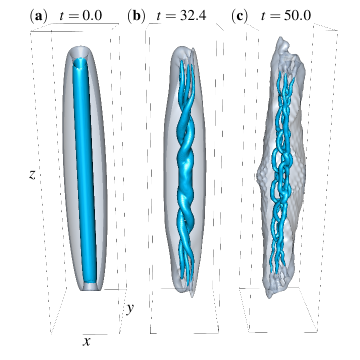
Figure 1: (Color online). The 3D isodensity plots show the time (in units of $\tau_{\mathrm{HO}}$) evolution of an initial $j=4$ multicharged vortex (a); notice the twisted unwinding of the vortex (b), which finally decays into four singly-charged ($j=1$) vortices (c) in the disordered, anisotropic state. The density isosurfaces representing the condensate and the vortices are respectively grey and blue. The axes directions are labeled as $x$, $y$, and $z$, in units of $\ell_{\mathrm{HO}}$.

IV Decay of single quadruply-charged vortex

The shape of the singly-charged vortex lines emerging from the decay of a multicharged vortex depends on where and when the decay starts. The singly-charged lines may be straight or intertwined (as reported here) depending on the perturbation’s symmetry and the local density homogeneity. If the perturbation is uniform and the density does not vary much in the $z$-direction, every point on the vortex unwinds at the same rate, and straight singly-charged vortex lines will emerge. However, if the density changes significantly along $z$, the unwinding takes place at different times at different positions, inducing intertwining, as discussed in Huhtamäki et al. (2006b).

The twisted vortex decay is shown in Fig. 1 and in the first movie in the Supplementary Material Sup . The main feature which is visible during the evolution are Kelvin waves. Kelvin waves consist of helical displacements of the vortex core axis, and play an important role in quantum turbulence Barenghi et al. (2014b); they have been recently experimentally identified in superfluid helium Fonda et al. (2014) and their presence has been recognized in atomic condensates Bretin et al. (2003); Smith et al. (2004). Considering Fig. 1, it is worth distinguishing the Kelvin waves which, in our case, emerge on parallel vortices from the decay of a multicharged vortex Möttönen et al. (2003); Mateo and Delgado (2006) in a confined geometry, from the Kelvin waves generated by the Crow instability Simula (2011) on anti-parallel vortices in a homogeneous condensate.

Our numerical experiments suggest that the decay of the multicharged vortex can be sped up. Imposing random fluctuations ($\leq 10\%$ of $|\psi|$) to the initial $j=4$ wave function does not significantly change the decay time scale, probably because the symmetry of the initial condition is not completely broken. A small displacement of the vortex core axis ($\approx 0.5~{}\ell_{\text{HO}}$) is more efficient, triggering the onset of the twisted unwinding in about 2.4$~{}\tau_{\text{HO}}$; a larger displacement ($\approx 0.2~{}\ell_{\text{HO}}$) reduces this time to 2.0$~{}\tau_{\text{HO}}$. Among the other methods which we have investigated, the most efficient is to gently squeeze the harmonic potential in the $xy$ plane by an amount $\omega_{x}/\omega_{y}=0.9$ when preparing the initial state in imaginary time, then resetting $\omega_{x}/\omega_{y}=1$ when propagating the GPE in real time; the squeeze triggers the onset of decay in only 1.0$~{}\tau_{\text{HO}}$. In the experiments, it is usually difficult to control perturbations well enough to reproducibly determine the time scale of decay.

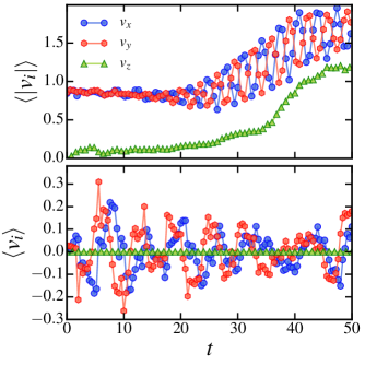
Figure 2: (Color online). Decay of quadruply-charged vortex (anisotropic state). Time evolution of average velocity components $v_{i}$ and $|v_{i}|$ (in units of $\ell_{ho}/\tau_{\text{HO}}$, where $i=x,y,z$) vs time (in units of $\tau_{\text{HO}}$). The symbol $\langle\cdots\rangle$ denotes the spatial average over the condensate.

Fig. 2 shows the time evolution of the (spatially) averaged velocity components and their magnitudes during the decay. The $x$- and $y$-components display oscillations which become large for $t>20~{}\tau_{\text{HO}}$, after the initial multicharged vortex has split. The $z$-component behaves differently because all vortices are aligned in the $z$-direction. For simplicity of reference, we call an ‘anisotropic state’ the resulting disordered vortex configuration.

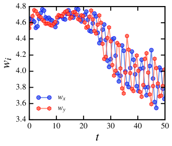
Figure 3: (Color online). Decay of quadruply-charged vortex (anisotropic state). Time (in units of $\tau_{\text{HO}}$) evolution of the condensate’s width $w_{i}$ (in units of $\ell_{\text{HO}}$).

V Decay of two antiparallel doubly-charged vortices

Now we exploit the twisted unwinding of a multicharged vortex as a convenient technique to generate turbulent vortex tangles which are relatively free of large density perturbations. We start by numerically imprinting anti-parallel, doubly-charged vortices as the initial state. One vortex is centered at position $(x,y)=(1.8~{}\ell_{\text{HO}},1.5~{}\ell_{\text{HO}})$ and the other at $(x,y)=(1.0~{}\ell_{\text{HO}},-1.3~{}\ell_{\text{HO}})$, as shown in Fig. 4(a). During the evolution, the vortices unwind, twist, move slightly forward due to the self-induced velocity field, and then reconnect, generating a turbulent state with only moderate density oscillations, as shown in Fig. 4(c).

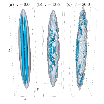
Figure 4: (Color online). Isodensity plots showing the evolution (with time $t$ in units of $\tau_{\text{HO}}$) of two initial doubly-charged ($j=2$) antiparallel vortices at $t=0~{}\tau_{\text{HO}}$ (a) into the turbulent quasi-isotropic state at $t=13.6~{}\tau_{\text{HO}}$ (b), which has finally decayed at $t=50~{}\tau_{\text{HO}}$ (c). The axes directions are labeled as $x$, $y$, and $z$, in units of $\ell_{\mathrm{HO}}$.

We analyze the turbulent state in terms of the spatial averages of the velocity components. At the beginning of the decay, we find $\langle|v_{y}|\rangle/\langle|v_{x}|\rangle\approx 1$ and (as expected, as vortices are initially aligned in the $z$-direction) $\langle|v_{z}|\rangle/\langle|v_{x}|\rangle\approx 0$. Fig. 5 (top) shows that, as the time proceeds, the vortex configuration becomes almost isotropic, indeed at $t=10~{}\tau_{\text{HO}}$ we have $\langle|v_{y}|\rangle/\langle|v_{x}|\rangle\approx 1.00$ and $\langle|v_{z}|\rangle/\langle|v_{x}|\rangle\approx 0.77$. For simplicity of reference, we call a ‘quasi-isotropic state’ the resulting disordered vortex configuration.

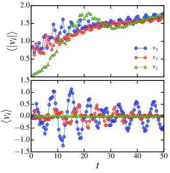
Figure 5: (Color online). Decay of antiparallel doubly-charged vortices (quasi-isotropic state). Time evolution of velocity components as in Fig. 2.

The oscillations of the transverse velocity components $v_{x}$ and $v_{y}$ appear practically in phase for the anisotropic case (see Fig. 2 (bottom)) and almost completely out of phase for the quasi-isotropic case (see Fig. 5 (bottom)), and these suggest the existence of collective modes. In order to properly identify these modes we have evaluated the time evolution of the condensate’s transverse widths $w_{x}$ and $w_{y}$ (found by adjusting Gaussian fits on $x$- and $y$-directions over the $z$-integrated density) for both cases. As can be seen in Fig. 3, the anisotropic case exhibits a quadrupolar mode, in which $w_{x}$ and $w_{y}$ oscillate out of phase in time. After performing a Fourier analysis of these quadrupolar oscillations we verified the mode’s frequency to be $\omega\sim\sqrt{2}\omega_{r}$, in agreement with theoretical predictions for a vortex-free cloud Stringari (1996). This mode is reminiscent of the unstable (quadrupolar) Bogoliubov mode that drives the decay of the initial multicharged vortex, as identified for an analogous 2D trapped system in Kuopanportti and Möttönen (2010). However, in the quasi-isotropic case, Fig. 6 shows that after $t\approx 10~{}\tau_{\text{HO}}$ there is a small ($\sim 0.2~{}\ell_{\text{HO}}$) in-phase oscillation of the widths (as opposed to the larger oscillations for the anisotropic case in Fig. 3). The latter can be identified as a breathing mode and (again, through a Fourier analysis) it was found to exhibit a characteristic frequency of $\omega\sim 2\omega_{r}$, also in agreement with theoretical predictions for a vortex-free cloud Stringari (1996); this value is expected to hold even for rapidly rotating trapped systems Watanabe (2006). These results, alongside a visual comparison of Figs. 1 and 4, show that the outer surface of the condensate is actually slightly less disturbed in the quasi-isotropic case. Our turbulent condensate (Fig. 3(c)) is clearly less ‘wobbly’ than condensates made turbulent via other stirring methods, notably Refs. White et al. (2010) and Parker and Adams (2005)).

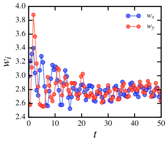
Figure 6: (Color online). Decay of antiparallel doubly-charged vortices (quasi-isotropic state). Time evolution of the condensate’s width.

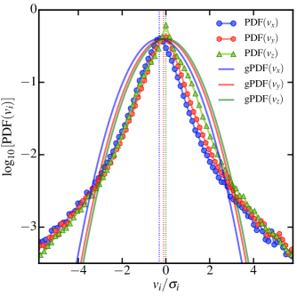
Figure 7: (Color online). Decay of antiparallel doubly-charged vortices (quasi-isotropic state). PDFs of velocity components $v_{i}$ ($i=x,y,z$ corresponding to blue, red, and green symbols respectively) plotted vs $v_{i}/\sigma_{i}$ (where $\sigma_{i}$ are the corresponding standard deviations) at $t=12.6~{}\tau_{\text{HO}}$. For reference, the solid curves are Gaussian fits (gPDFs) with standard deviations $\sigma_{x}=1.8$, $\sigma_{y}=1.7$ and $\sigma_{z}=1.4$, and mean values (plotted as vertical lines near the origin) $\mu_{x}=-0.3$, $\mu_{y}=-0.1$ and $\mu_{z}=0.0$.

We proceed and analyze the distribution of values of the turbulent velocity components (Fig. 7). We find that the probability density functions (PDFs, or normalized histograms) display the typical power-law scaling ${\rm PDF}(v_{i})\sim v_{i}^{\alpha_{i}}$ ($i=x,y,z$) where $\alpha_{x}\approx-2.97$, $\alpha_{y}\approx-2.95$, $\alpha_{z}\approx-3.20$, in agreement with findings in larger condensates White et al. (2010). Such power-law scaling, characteristic of quantum turbulence and observed in helium experiments Paoletti et al. (2008), contrasts the Gaussian PDFs which are typical of ordinary turbulence. The difference between power-law and Gaussian statistics is important at high velocities (power-law PDFs have larger values in the tails) and arises from the quantization of vorticity (which creates very large velocity $v=\kappa/(2\pi r)$ for $r\to 0$). For the sake of comparison, Fig. 7 also displays Gaussian fits gPD .

VI Identification of the turbulence

The two disordered vortex states, anisotropic and quasi-isotropic, produced respectively by the decay of a single quadruply-charged vortex (Section IV) and by decay of two antiparallel doubly-charged vortices (Section V) are clearly different. In the anisotropic state, all vortex lines are aligned in the same direction, and the net nonzero angular momentum constrains the flow. In the quasi-isotropic state, the oscillations of the transverse velocity components are three times larger, suggesting the presence of high-velocity events (vortex reconnections between Kelvin waves growing on opposite-oriented vortices) which are the hallmarks of turbulence. Moreover, in the quasi-isotropic state, the zero angular momentum of the initial configuration allows a redistribution of the velocity field, making the amplitudes of the three velocity components almost equal; indeed, after the initial vortex has split ($t\approx 10~{}\tau_{\text{HO}}$), the axial velocity $\langle|v_{z}|\rangle\approx 0.9~{}\ell_{\text{HO}}/\tau_{\text{HO}}$, is not much smaller than the transverse velocity $\langle|v_{x}|\rangle\approx 1.2~{}\ell_{\text{HO}}/\tau_{\text{HO}}$ and $\langle|v_{y}|\rangle\approx~{}1.1~{}\ell_{\text{HO}}/\tau_{\text{HO}}$. On the contrary, in the anisotropic state, at the same stage ($t\approx 10~{}\tau_{\text{HO}}$), the axial velocity component is much smaller than the transverse components. In other words, the velocity field which results from the decay of the antiparallel doubly-charged vortex state is indeed almost isotropic.

Since there is not yet a precise definition of turbulence, in principle both disordered states investigated here could be considered somewhat ‘turbulent’. However at this early stage of investigation, we want to make conceptual connections to the simple isotropic cases known in the literature (in particular, the Kolmogorov and Vinen types of turbulence). Therefore hereafter we concentrate on the quasi-isotropic state.

The next question is whether the quasi-isotropic state is ‘turbulent’ in the sense of ordinary turbulence or in comparison with turbulent superfluid helium. To find the answer, we turn to the workhorse of statistical physics: the correlation function.

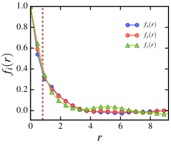
Figure 8: (Color online). Decay of antiparallel doubly-charged vortices (quasi-isotropic state). Longitudinal correlation functions $f_{i}(r)$ ($i=x,y,z$) vs $r$ (in units of $\ell_{\text{HO}}$) at $t=13~{}\tau_{\text{HO}}$. The vertical dashed lines indicate the length $\ell_{c}$ over which the velocity field is highly correlated, as defined in Eq.(4).

The quantity which measures the degree of randomness of a turbulent flow is the (normalized) longitudinal correlation functions Stagg et al. (2016); Davidson (2004), defined by

$$f_{i}(r)=\frac{\left<v_{i}(\mathbf{x}+r{{\hat{\bf e}}_{i}})v_{i}(\mathbf{x})\right>}{\left<v_{i}(\mathbf{x})^{2}\right>},$$ (3)

where the symbol $\langle\cdots\rangle$ denotes average over $\mathbf{x}$, and ${\hat{\bf e}}_{i}$ is the unit vector in the direction $i=x,y,z$. The distance $r$ is limited by the size of the BEC, approximately the transverse and axial Thomas-Fermi radii $d_{\text{TF}}=4.2~{}\ell_{\text{HO}}$ and $D_{\text{TF}}=32.6~{}\ell_{\text{HO}}$. From the longitudinal correlation function one obtains the integral length scale

$$\ell_{c}=\int_{0}^{\infty}f_{i}(r)dr.$$ (4)

In fluid dynamics, $\ell_{c}$ represents the size of the large eddies. In our case, $\ell_{c}$ is the length scale over which the velocity field is highly correlated. Fig. 8 shows that the correlation functions drop to only $\approx 10\%$ at distances of the order of the average separation between the vortex lines, $\ell\approx 6.1~{}\ell_{\text{HO}}$; the last quantity is estimated as $\ell\approx L^{-1/2}$ from the measurement of the vortex line density $L$ (the vortex length per unit volume). Physically, this lack of correlation means that the vortex lines are randomly oriented with respect to each other. The analysis of the correlation function therefore suggests that the turbulent velocity field arising from the decay of antiparallel doubly-charged vortices is essentially a random flow.

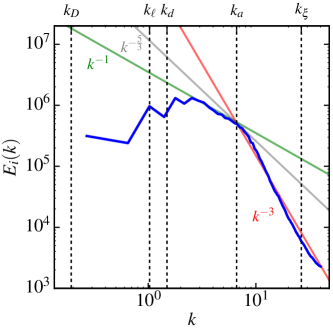
Figure 9: (Color online). Decay of two antiparallel doubly-charged vortices (quasi-isotropic state). Incompressible kinetic energy spectrum $E_{i}(k)$ (arbitrary units) vs wavenumber $k$ (in units of $\ell_{\text{HO}}^{-1}$) at $t=12.8~{}\tau_{\text{HO}}$. The vertical lines mark the wavenumbers corresponding to the healing length $\xi=0.24~{}\ell_{\text{HO}}$, the vortex core size $a=0.96~{}\ell_{\text{HO}}$, the average distance between vortex lines $\ell_{v}=6.10~{}\ell_{\text{HO}}$, the radial and axial Thomas-Fermi radii $d_{\text{TF}}=4.21~{}\ell_{\text{HO}}$ and $D_{\text{TF}}=32.64~{}\ell_{\text{HO}}$. Red, grey and green lines mark the power laws $k^{-3}$, $k^{-5/3}$ and $k^{-1}$ respectively.

This result implies that the distribution of the kinetic energy over the length scales, or energy spectrum $E(k)$ (where the wavenumber $k$ represents the inverse length scale), should be very different from the celebrated Kolmogorov scaling, $E(k)\sim k^{-5/3}$, which is observed in classical turbulence and implies a particular structure of the flow. The importance of the Kolmogorov scaling is that it is the signature of a nonlinear cascade mechanism which transfers energy from large length scales to small length scales. Besides ordinary turbulence, the classical Kolmogorov scaling has been observed in helium experiments Maurer and Tabeling (1998); Salort et al. (2010) when the turbulence is generated by grids in wind tunnels or by counter-rotating propellers. Numerical simulations Baggaley et al. (2012a) revealed that the Kolmogorov scaling is associated with the presence of large-scale polarization (bundles) of vortex lines which become locally parallel to each other; the bundles locally create a net average rotation over length scales larger than $\ell$, thus building up energy at wavenumbers $k<k_{\ell}=2\pi/\ell$ (the hydrodynamical range).

To compute the energy spectrum $E(k)$ of our turbulent condensate, we use a standard procedure Nore et al. (1997) to extract the incompressible kinetic energy from the total energy, obtaining Fig. 9. To interpret the figure, we mark with vertical lines the wavenumbers $k_{\xi}=2\pi/\xi$, $k_{a}=2\pi/a$, $k_{\ell}=2\pi/\ell$, $k_{d}=2\pi/d_{\text{TF}}$ and $k_{D}=2\pi/D_{\text{TF}}$ corresponding to the healing length $\xi$, the vortex core radius $a$, the average vortex separation $\ell$, and the radial and axial Thomas-Fermi radii, $d_{\text{TF}}$ and $D_{\text{TF}}$. Fig. 9 clearly shows that, at the hydrodynamical length scales $k<k_{\ell}$ the energy spectrum is not of Kolmogorov type: under the classical $k^{-5/3}$ scaling, substantially more energy would be contained in the small $k$ region. Instead, over a wide range of wavenumbers up to $k_{a}$, we observe the $E(k)\sim k^{-1}$ spectrum which is characteristic of an isolated straight vortex line. This means that, at distances less than $\ell$, the velocity field is dominated by the nearest vortex in the vicinity of the point of observation - the effects of all the other vortices in a random tangle canceling each other out. Fig. 9 is therefore consistent with the random flow interpretation which results from the analysis of the correlation functions. It is also worth noticing that the $E(k)\sim k^{-3}$ scaling which appears in the region $k_{a}<k<k_{\xi}$ is characteristic of the vortex core Krstulovic and Brachet (2010); Bradley and Anderson (2012).

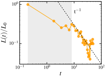
Figure 10: (Color online). Time evolution of vortex line density ($t$ in units of $\tau_{\text{HO}}$). The shaded area corresponds to the time elapsed for the decay of the two antiparallel multiply-charged vortices, $t\approx 8~{}\tau_{\text{HO}}$, after which we only see singly quantized vortices in the system in the quasi-isotropic state.

Besides the correlation function and the energy spectrum, further insight into the nature of our turbulence is acquired by measuring the temporal decay of the vortex line density $L(t)$. This decay is caused by sound radiated away by vortices as they accelerate about each other Leadbeater et al. (2003) or reconnect Leadbeater et al. (2001) with each other. Fig. 8 shows that, at large $t$, the decay is consistent with the form $L(t)\sim t^{-1}$, as reported for a larger spherical condensate White et al. (2010); the decaying turbulence is shown in the second movie in the Supplementary Material Sup . The $L(t)\sim t^{-1}$ decay is characteristic of the ‘Vinen’ turbulence regime (also called ‘ultra-quantum regime’) which was generated in superfluid helium by Walmsley & Golov Walmsley and Golov (2008) by short injections of vortex rings; long injections generated a ‘Kolmogorov’ (or ‘quasi-classical’) regime which decayed as $L(t)\sim t^{-3/2}$. Numerical simulations Baggaley et al. (2012b) of Walmsley & Golov’s experiment revealed that (at large $k$ within the hydrodynamical range $k<k_{\ell}$) ‘Vinen turbulence’ (decaying as $L(t)\sim t^{-1}$) has spectrum $E(k)\sim k^{-1}$ and ‘Kolmogorov turbulence’ (decaying as $L(t)\sim t^{-3/2}$) has spectrum $E(k)\sim k^{-5/3}$.

The distinction between ‘Vinen turbulence’ and ‘Kolmogorov turbulence’, first proposed by Volovik Volovik (2003), seems to be characteristic of superfluids. It is now understood that Vinen’s pioneering experiments Vinen (1957) on counterflow heat transfer in superfluid helium generated ‘Vinen turbulence’: this was demonstrated by numerical models of counterflow turbulence Baggaley et al. (2012c) which produced the expected $E(k)\sim k^{-1}$ energy spectrum and the $L(t)\sim t^{-1}$ vortex line density decay, which is the large-$t$ decaying solution of the equation $dL/dt\sim-L^{2}$ proposed by Vinen on simple physical arguments to model a random-like flow.

A recent work Stagg et al. (2016) has examined the properties of the turbulence following a thermal quench of a Bose gas. It found that topological defects created by the Kibble-Zurek mechanism evolve into a turbulent vortex tangle Berloff and Svistunov (2002) which eventually decays into a vortex free state. During the decay, which has the form $L(t)\sim t^{-1}$, the energy spectrum is $E(k)\sim k^{-1}$ and the correlation functions drop to few percent over the distance $\ell$. The thermal quench is therefore another clear example of ‘Vinen turbulence’.

VII Conclusion

In this work we have explored the decay of initially imprinted multicharged vortices as a method to generate turbulence in a trapped Bose-Einstein condensate which is relatively free from large surface oscillations and fragmentation. We have examined the decay of two multicharged vortex systems, in a typical cigar-shaped harmonically confined atomic Bose-Einstein condensate. The first (a quadruply charged vortex) led to the disordered, anisotropic vortex state. The second (two antiparallel doubly-charged vortices) generated helical Kelvin waves on opposite oriented vortex lines which reconnected, creating a second disordered, quasi-isotropic vortex state. Looking for similarities with ordinary turbulence in its simplest possible forms - in particular with the property of isotropy - we have concentrated the attention on the quasi-isotropic state, and carefully considered in which sense it is turbulent.

This question is subtle. In classical physics, turbulence implies a large range of length scales which are all excited and interact nonlinearly. In ordinary fluids, the presence and the intensity of turbulence is inferred from the Reynolds number $\rm Re$, which must be sufficiently large (typically few thousands, depending on the problem) for turbulence to exist. But the Reynolds number has two definitions. The first definition is

$${\rm Re}=\frac{uD}{\nu},$$ (5)

where $D$ is the system’s large length scale, i.e. the system’s size or the size of the energy containing eddies, $u$ is the flow’s velocity at that large scale, and $\nu$ is the kinematic viscosity; this definition follows directly from the Navier-Stokes equation, and measures the ratio of the magnitudes of inertial and viscous forces acting on a fluid parcel. The definition makes apparent why large scale (e.g. geophysical) flows are always turbulent, and why microfluids flows are not (indeed, with microfluids one has to rely on chaos, not turbulence, for achieving any desired mixing). The second definition assumes Kolmogorov theory, and is

$${\rm Re}=\left(\frac{D}{\eta}\right)^{4/3}$$ (6)

(where $\eta$ is the length scale of viscous dissipation). This definition measures the degree of separation between the large length scale (at which energy is typically injected) and the small length scale (at which energy is dissipated). In the context of condensates, the two definitions clash with each other: The first definition implies that $\rm Re$ is infinite (because the viscosity is zero), and the second that $\rm Re$ is not much larger than unity (because the size of a typical condensate is larger, but not orders of magnitude larger, than the healing length, which can be considered the length scale at which acoustic dissipation of kinetic energy occurs). Although interesting work is in progress to identify a definition of Reynolds number suitable for a superfluid system (for example exploring dynamical similarities Reeves et al. (2015)), to answer the question which we asked, at this stage, we have to leave the Reynolds number and proceed in other ways.

We have therefore carefully examined the properties of the disordered, quasi-isotropic state in terms of velocity statistics, energy spectrum, correlation function and temporal decay, and compared them to the properties of ordinary turbulence and of turbulent superfluid helium. Clearly, the quasi-isotropic state does not compare well with the properties of ordinary turbulence. Despite the limited range of length scales available in a small BEC, we conclude that, in the decay of the two antiparallel doubly-charged vortices, the quasi-isotropy of our disordered state, the short correlation length, the $E(k)\sim k^{-1}$ scaling of the energy spectrum at the hydrodynamical length scales, and the $L(t)\sim t^{-1}$ temporal behavior of the decay, identify our disordered, quasi-isotropic vortex state as an example of the ‘Vinen turbulent regime’ discovered in superfluid helium at low temperatures.

The nature of the disorder, or turbulence, in the anisotropic case generated by the decay of the single quadruply-charged vortex will be the subject of future investigations: one should vary the amount of polarization and study fluctuations of the velocity field over the mean rotating flow. There are no numerical studies yet of such turbulence in trapped Bose systems, and (because of the role played by boundaries in the spin-down of viscous flows) no immediate classical analogies, so this case is less straightforward to analyze; spin-down dynamics experiments in superfluid helium Walmsley et al. (2008); Hosio et al. (2013, 2012) should be the main reference systems.

Future work will also address the next natural question: can the classical Kolmogorov regime be achieved in much larger condensates under suitable forcing at the largest length scale, as suggested by some numerical simulations Kobayashi and Tsubota (2007), thus identifying the cross over between Vinen and Kolmogorov turbulence?

References

- Barenghi et al. (2014a) C. F. Barenghi, V. S. L’vov, and P.-E. Roche, Proceedings of the National Academy of Sciences 111, 4683 (2014a).
- Frisch (1995) U. Frisch, Turbulence: The legacy of A. N. Kolmogorov., by Frisch, U.. Cambridge University Press, Cambridge (UK) (1995).
- Hänninen and Baggaley (2014) R. Hänninen and A. W. Baggaley, Proceedings of the National Academy of Sciences 111, 4667 (2014).
- Walmsley and Golov (2008) P. M. Walmsley and A. I. Golov, Phys. Rev. Lett. 100, 245301 (2008).
- Barenghi et al. (2016) C. F. Barenghi, Y. A. Sergeev, and A. W. Baggaley, Scientific Reports 6 (2016), doi:10.1038/srep35701.
- Aioi et al. (2011) T. Aioi, T. Kadokura, T. Kishimoto, and H. Saito, Phys. Rev. X 1, 021003 (2011).
- Davis et al. (2009) M. C. Davis, R. Carretero-González, Z. Shi, K. J. H. Law, P. G. Kevrekidis, and B. P. Anderson, Phys. Rev. A 80, 023604 (2009).
- Madison et al. (2000) K. W. Madison, F. Chevy, W. Wohlleben, and J. Dalibard, Phys. Rev. Lett. 84, 806 (2000).
- Raman et al. (2001) C. Raman, J. R. Abo-Shaeer, J. M. Vogels, K. Xu, and W. Ketterle, Phys. Rev. Lett. 87, 210402 (2001).
- Freilich et al. (2010) D. V. Freilich, D. M. Bianchi, A. M. Kaufman, T. K. Langin, and D. S. Hall, Science 329, 1182 (2010).
- Tsatsos et al. (2016) M. C. Tsatsos, P. E. Tavares, A. Cidrim, A. R. Fritsch, M. A. Caracanhas, F. E. A. dos Santos, C. F. Barenghi, and V. S. Bagnato, Physics Reports 622, 1 (2016).
- Barenghi et al. (2014b) C. F. Barenghi, L. Skrbek, and K. R. Sreenivasan, Proceedings of the National Academy of Sciences 111, 4647 (2014b).
- Skrbek and Sreenivasan (2012) L. Skrbek and K. R. Sreenivasan, Physics of Fluids 24, 011301 (2012).
- Neely et al. (2010) T. W. Neely, E. C. Samson, A. S. Bradley, M. J. Davis, and B. P. Anderson, Phys. Rev. Lett. 104, 160401 (2010).
- White et al. (2012) A. C. White, C. F. Barenghi, and N. P. Proukakis, Phys. Rev. A 86, 013635 (2012).
- White et al. (2014) A. C. White, N. P. Proukakis, and C. F. Barenghi, Journal of Physics: Conference Series 544, 012021 (2014).
- Kwon et al. (2014) W. J. Kwon, G. Moon, J.-y. Choi, S. W. Seo, and Y.-i. Shin, Phys. Rev. A 90, 063627 (2014).
- Stagg et al. (2015) G. W. Stagg, A. J. Allen, N. G. Parker, and C. F. Barenghi, Phys. Rev. A 91, 013612 (2015).
- Allen et al. (2014) A. J. Allen, N. G. Parker, N. P. Proukakis, and C. F. Barenghi, Phys. Rev. A 89, 025602 (2014).
- Cidrim et al. (2016) A. Cidrim, F. E. A. dos Santos, L. Galantucci, V. S. Bagnato, and C. F. Barenghi, Phys. Rev. A 93, 033651 (2016).
- Henn et al. (2009) E. A. L. Henn, J. A. Seman, G. Roati, K. M. F. Magalhães, and V. S. Bagnato, Phys. Rev. Lett. 103, 045301 (2009).
- Kobayashi and Tsubota (2007) M. Kobayashi and M. Tsubota, Phys. Rev. A 76, 045603 (2007).
- White et al. (2010) A. C. White, C. F. Barenghi, N. P. Proukakis, A. J. Youd, and D. H. Wacks, Phys. Rev. Lett. 104, 075301 (2010).
- Weiler et al. (2008) C. N. Weiler, T. W. Neely, D. R. Scherer, A. S. Bradley, M. J. Davis, and B. P. Anderson, Nature 455, 948 (2008).
- Chomaz et al. (2015) L. Chomaz, L. Corman, T. Bienaimé, R. Desbuquois, C. Weitenberg, S. Nascimbène, J. Beugnon, and J. Dalibard, Nature communications 6 (2015).
- Lamporesi et al. (2013) G. Lamporesi, S. Donadello, S. Serafini, F. Dalfovo, and G. Ferrari, Nature Physics 9, 656 (2013).
- Navon et al. (2015) N. Navon, A. L. Gaunt, R. P. Smith, and Z. Hadzibabic, Science 347, 167 (2015).
- Parker and Adams (2005) N. Parker and C. Adams, Phys. Rev. Lett. 95, 145301 (2005).
- Barenghi and Parker (2016) C. Barenghi and N. Parker, A Primer on Quantum Fluids, SpringerBriefs in Physics (Springer International Publishing, 2016).
- Shin et al. (2004) Y.-i. Shin, M. Saba, M. Vengalattore, T. Pasquini, C. Sanner, A. Leanhardt, M. Prentiss, D. Pritchard, and W. Ketterle, Phys. Rev. Lett. 93, 160406 (2004).
- Kumakura et al. (2006) M. Kumakura, T. Hirotani, M. Okano, Y. Takahashi, and T. Yabuzaki, Phys. Rev. A 73, 063605 (2006).
- Okano et al. (2007) M. Okano, H. Yasuda, K. Kasa, M. Kumakura, and Y. Takahashi, Journal of Low Temperature Physics 148, 447 (2007).
- Isoshima et al. (2007) T. Isoshima, M. Okano, H. Yasuda, K. Kasa, J. A. M. Huhtamäki, M. Kumakura, and Y. Takahashi, Phys. Rev. Lett. 99, 200403 (2007).
- Pu et al. (1999) H. Pu, C. Law, J. Eberly, and N. Bigelow, Phys. Rev. A 59, 1533 (1999).
- Möttönen et al. (2003) M. Möttönen, T. Mizushima, T. Isoshima, M. M. Salomaa, and K. Machida, Phys. Rev. A 68, 023611 (2003).
- Huhtamäki et al. (2006a) J. A. M. Huhtamäki, M. Möttönen, and S. M. M. Virtanen, Phys. Rev. A 74, 063619 (2006a).
- Huhtamäki et al. (2006b) J. A. M. Huhtamäki, M. Möttönen, T. Isoshima, V. Pietilä, and S. M. M. Virtanen, Phys. Rev. Lett. 97, 110406 (2006b).
- Mateo and Delgado (2006) A. M. n. Mateo and V. Delgado, Phys. Rev. Lett. 97, 180409 (2006).
- Kuwamoto et al. (2010) T. Kuwamoto, H. Usuda, S. Tojo, and T. Hirano, Journal of the Physical Society of Japan 79, 034004 (2010).
- Kuopanportti and Möttönen (2010) P. Kuopanportti and M. Möttönen, Phys. Rev. A 81, 033627 (2010).
- Nakahara et al. (2000) M. Nakahara, T. Isoshima, K. Machida, S.-i. Ogawa, and T. Ohmi, Physica B: Condensed Matter 284, 17 (2000).
- Leanhardt et al. (2002) A. Leanhardt, A. Görlitz, A. Chikkatur, D. Kielpinski, Y.-i. Shin, D. Pritchard, and W. Ketterle, Phys. Rev. Lett. 89, 190403 (2002).
- Kawaguchi and Ohmi (2004) Y. Kawaguchi and T. Ohmi, Phys. Rev. A 70, 043610 (2004).
- Dennis et al. (2013) G. R. Dennis, J. J. Hope, and M. T. Johnsson, Computer Physics Communications 184, 201 (2013).
- (45) See supplemental material at [URL will be inserted by the publisher]. Movie 1: real decay of a multi-charged vortex line. Movie 2: real decay of two antiparallel doubly-charged vortex lines.
- Fonda et al. (2014) E. Fonda, D. P. Meichle, N. T. Ouellette, S. Hormoz, and D. P. Lathrop, Proceedings of the National Academy of Sciences 111, 4707 (2014).
- Bretin et al. (2003) V. Bretin, P. Rosenbusch, F. Chevy, G. Shlyapnikov, and J. Dalibard, Phys. Rev. Lett. 90, 100403 (2003).
- Smith et al. (2004) N. Smith, W. Heathcote, J. Krueger, and C. Foot, Phys. Rev. Lett. 93, 080406 (2004).
- Simula (2011) T. P. Simula, Phys. Rev. A 84, 021603 (2011).
- Stringari (1996) S. Stringari, Phys. Rev. Lett. 77, 2360 (1996).
- Watanabe (2006) G. Watanabe, Phys. Rev. A 73, 013616 (2006).
- Paoletti et al. (2008) M. S. Paoletti, M. E. Fisher, K. R. Sreenivasan, and D. P. Lathrop, Phys. Rev. Lett. 101, 154501 (2008).
- (53) The definition is where and () are the mean values and the standard deviations respectively.
- Stagg et al. (2016) G. W. Stagg, N. G. Parker, and C. F. Barenghi, Phys. Rev. A 94, 053632 (2016).
- Davidson (2004) P. Davidson, Turbulence: An Introduction for Scientists and Engineers (OUP Oxford, 2004).
- Maurer and Tabeling (1998) J. Maurer and P. Tabeling, EPL (Europhysics Letters) 43, 29 (1998).
- Salort et al. (2010) J. Salort, C. Baudet, B. Castaing, B. Chabaud, F. Daviaud, T. Didelot, P. Diribarne, B. Dubrulle, Y. Gagne, F. Gauthier, A. Girard, B. Hébral, B. Rousset, P. Thibault, and P.-E. Roche, Physics of Fluids 22, 125102 (2010), http://dx.doi.org/10.1063/1.3504375 .
- Baggaley et al. (2012a) A. W. Baggaley, J. Laurie, and C. F. Barenghi, Phys. Rev. Lett. 109, 205304 (2012a).
- Nore et al. (1997) C. Nore, M. Abid, and M. Brachet, Phys. Rev. Lett. 78, 3896 (1997).
- Krstulovic and Brachet (2010) G. Krstulovic and M. Brachet, Phys. Rev. Lett. 105, 129401 (2010).
- Bradley and Anderson (2012) A. S. Bradley and B. P. Anderson, Phys. Rev. X 2, 041001 (2012).
- Leadbeater et al. (2003) M. Leadbeater, D. Samuels, C. Barenghi, and C. Adams, Phys. Rev. A 67, 015601 (2003).
- Leadbeater et al. (2001) M. Leadbeater, T. Winiecki, D. Samuels, C. Barenghi, and C. Adams, Phys. Rev. Lett. 86, 1410 (2001).
- Baggaley et al. (2012b) A. W. Baggaley, C. F. Barenghi, and Y. A. Sergeev, Phys. Rev. B 85, 060501 (2012b).
- Volovik (2003) G. E. Volovik, JETP Letters 78, 533 (2003).
- Vinen (1957) W. Vinen, in Proceedings of the Royal Society of London A: Mathematical, Physical and Engineering Sciences, Vol. 240 (The Royal Society, 1957) pp. 114–127.
- Baggaley et al. (2012c) A. W. Baggaley, L. Sherwin, C. F. Barenghi, and Y. Sergeev, Phys. Rev. B 86, 104501 (2012c).
- Berloff and Svistunov (2002) N. G. Berloff and B. V. Svistunov, Phys. Rev. A 66, 013603 (2002).
- Reeves et al. (2015) M. Reeves, T. Billam, B. P. Anderson, and A. Bradley, Phys. Rev. Lett. 114, 155302 (2015).
- Walmsley et al. (2008) P. Walmsley, A. Golov, H. Hall, W. Vinen, and A. Levchenko, Journal of Low Temperature Physics 153, 127 (2008).
- Hosio et al. (2013) J. Hosio, V. Eltsov, P. Heikkinen, R. Hänninen, M. Krusius, and V. L’vov, Nature communications 4, 1614 (2013).
- Hosio et al. (2012) J. Hosio, V. Eltsov, M. Krusius, and J. Mäkinen, Phys. Rev. B 85, 224526 (2012).