Connected and Disconnected Contractions in Pion-Pion Scattering

Abstract

We show that the interplay of chiral effective field theory and lattice QCD can be used in the evaluation of so-called disconnected diagrams, which appear in the study of the isoscalar and isovector channels of pion-pion scattering and have long been a major challenge for the lattice community. By means of partially-quenched chiral perturbation theory, we distinguish and analyze the effects from different types of contraction diagrams to the pion-pion scattering amplitude, including its scattering lengths and the energy-dependence of its imaginary part. Our results may be used to test the current degree of accuracy of lattice calculation in the handling of disconnected diagrams, as well as to set criteria for the future improvement of relevant lattice computational techniques that may play a critical role in the study of other interesting QCD matrix elements.

1 Introduction

Quantum Chromodynamics (QCD) is well-accepted as the fundamental field theory of the strong interaction. However, a direct comparison between theoretical predictions and experiments is extremely difficult at low energies (e.g. $E\ll 1$ GeV) due to the non-perturbative nature of the theory in that regime, making first-principle calculations very challenging. Lattice QCD is currently the most promising approach to study the low-energy behavior of QCD from first principles. On the other hand, low-energy effective field theories (EFTs) of QCD are very useful in understanding the analytic behavior of the theory, but can also be used to make sharp predictions once the correspoding low-energy constants have been determined. Chiral Perturbation Theory (ChPT) is an example of such kind, based on the fact that chiral symmetry is spontaneously broken at the hadronic scale and the lowest-lying pseudoscalar mesons play the role of Goldstone bosons.

Meson-meson scattering is a perfect testing ground to check the validity of different effective approaches to low-energy QCD. Large amounts of data on phase shifts have been accumulated in various channels of isospins and partial waves, covering a wide range of energy from $2M_{\pi}$ up to 1.5 GeV or higher. The quest to reproduce these phase shifts and, in particular, account for the contributions from resonance states, sets a great challenge for both the lattice and EFT communities. The low-energy $\pi\pi$ scattering has been calculated up to two-loop order in ChPT [1], and the phenomenologically most precise and model-independent description comes from the dispersion-relation treatments using the Roy equations matched to ChPT [2, 3]. On the lattice side, tremendous effort has been spent over decades in the calculation of $\pi\pi$ scattering lengths and phase shifts on the lattice. These works cover the scattering at $I=2$ [4, 5, 6, 7, 8, 9, 10, 11, 12, 13, 14, 15, 16, 17], $I=1$ [18, 19, 20, 21, 22, 23, 24, 25, 26, 27, 28, 29] and $I=0$ [4, 5, 30, 31, 32, 33] channels.

The difficulty in the lattice study of $\pi\pi$ scattering increases with the decrease in isospin, partly due to the differences in the involved types of quark contraction diagrams. In general, one is calculating a four-point correlation function $\left\langle\mathcal{O}_{\pi\pi}(t)\mathcal{O}_{\pi\pi}^{\prime\dagger}(t^{\prime})\right\rangle$ where each of $\mathcal{O}$ and $\mathcal{O}^{\prime}$ is an interpolating field operator of the form $\bar{q}\Gamma^{i}q(\bm{x},t)\,\bar{q}\Gamma^{j}q(\bm{y},t)$, representing a state of two pions at different spacial sites. These correlation functions can be decomposed into distinct sets of diagrams according to different Wick contractions of the quark fields. In particular, contraction diagrams involving quark propagators starting from and ending at points with the same time coordinates appear to be extremely noisy, which makes the extraction of lattice signals very difficult. Such contractions are called disconnected diagrams. Therefore, the $I=2$ scattering amplitude that does not involve such contractions is relatively easy to calculate. The $I=1$ channel is more difficult while the $I=0$ channel was a real challenge for a long time. With the development of new lattice techniques (e.g. the implementation of all-to-all propagators [34, 35, 36]), the study of isoscalar channel becomes possible, but at this stage it is safe to say that the level of understanding is still relatively immature compared to the $I=2$ channel. Furthermore, the problem of handling disconnected diagrams also appears in the lattice computation of many other interesting hadronic observables, such as the parity-odd pion-nucleon coupling [37]. It would thus be helpful to gain insights from the EFTs about the analytical behavior of different contraction diagrams so that we have a measure of how important various kinds of contraction diagrams could be. This would provide a gauge of how accurate lattice calculation can handle such behavior. For $\pi\pi$ scattering, the first attack on such a problem was performed in Ref. [38], where different types of contractions were ordered according to both the $1/N_{c}$ and the chiral expansion. However, therein the involved contractions were only computed at the leading order (LO) of ChPT whose use is limited as contractions involving more than one closed quark loops vanish at that order.

Partially-quenched chiral perturbation theory (PQChPT) [39, 40, 41, 42, 43] (for reviews, see [44, 45]) turns out to be an excellent candidate to fulfill the task mentioned above and improve the calculations in Ref. [38] to higher orders in order to get a quantitative control of all relevant contractions. Its underlying theory, namely the partially-quenched QCD (PQQCD), was first invented as an aid for lattice QCD to deal with light fermion loops. Early numerical simulations of lattice QCD were bothered by the difficulty to include loops of light quarks (which is equivalent to the computation of the fermion determinant). The partially-quenched approximation, namely to take the mass of quarks that appear in closed loops (also known as “dynamical quarks” or “sea quarks”) to be unphysically large, was carried out to reduce the computational effort. The outcome, however, has to be extrapolated to the region where the sea quark masses take their physical values. This is made possible by PQQCD which first separates the usual fermionic quarks into “valence” and “sea” quarks, and introduces, for each valence quark, a degenerate bosonic quark (known as “ghost quark”) that cancels all the closed-loop contribution of the valence quark. With such an arrangement, the masses of the quarks appearing in the external legs and in closed loops can be made different. One can go one step further to introduce PQChPT which is the effective field theory of PQQCD at low energy. Since the outcomes of PQChPT are analytic functions of sea quarks masses, one could match them to lattice results at unphysical sea quark masses and simply extrapolate them to the physical region.

Computational techniques on the lattice have improved significantly nowadays and many calculations can be done without using the partially-quenched approximation. Despite that, PQChPT still continues to be very useful in the understanding of, and to aid, lattice calculations. The basic idea is that, by suitably choosing the type of quarks that appear in external legs, one is able to access any specific type of Wick contraction one wants, provided that the valence quarks are degenerate with the sea quarks. Also, when one considers loop diagrams, the inclusion of ghost quarks is still required so that the number of degrees of freedom (DOFs) that appear in the loop is the same as that in the original theory. This strategy has been used to study the connected and disconnected diagrams in, e.g., hadronic vacuum polarization [48] or the pion scalar form factor [49]. In this work, we demonstrate exactly how PQChPT can be applied to distinguish contributions from different Wick contractions to the $\pi\pi$ scattering amplitude. This task has been carried out at the LO, i.e. $\mathcal{O}\!\left(p^{2}\right)\!\,$, in Ref. [38] and here we want to study the complete next-to-leading order (NLO), i.e. $\mathcal{O}\!\left(p^{4}\right)\!\,$, contributions. For the sake of simplicity, we work in the SU(2) version of ChPT, but a generalization to SU(3) is straightforward.

This work is arranged as follows: In Section 2 we review the basic setup of SU$(4|2)$ PQQCD and PQChPT. Section 3 contains a classification of all types of quark contraction diagrams that contribute to the $\pi\pi$ scattering in all isospin channels. In Section 4 we provide the analytic expressions of the scattering amplitudes contributed by each type of contraction up to NLO in PQChPT while in Section 5 we show some numerical results, with a special emphasis to the contribution from each contraction diagram to the partial wave amplitudes. The final conclusions are given in Section 6. The appendices contain analytic expressions of scattering lengths decomposed into contributions from different types of contractions, as well as PQChPT in a formulation slightly different from the one discussed in the main text.

2 Basic setup

We will show in the next section that the simplest PQQCD that is relevant to our work has a flavor-SU$(4|2)$ structure. Therefore, we start with a very brief review of the theory. The quarks are grouped into a fundamental representation of SU$(4|2)$:

$$Q=\left(u\>d\>j\>k\>|\>\tilde{j}\>\tilde{k}\right)^{T}.$$ (1)

Here, $u,d$ are the dynamical quarks, $j,k$ and $\tilde{j},\tilde{k}$ are the valence and ghost quarks, respectively. The PQQCD Lagrangian is given by

$$\mathcal{L}=\bar{Q}(i\not{D}-M)Q-\frac{1}{4}G^{a\mu\nu}G^{a}_{\mu\nu}.$$ (2)

For our purpose in this paper, all quarks are taken to be degenerate. Therefore, the quark mass matrix is simply $M=\mathrm{diag}\left(m_{q},m_{q},m_{q},m_{q},m_{q},m_{q}\right)$.

The massless PQQCD Lagrangian is invariant under $Q_{L/R}\to U_{L/R}Q_{L/R}$, where $U_{L/R}\in$SU$(4|2)_{L/R}$ are elements of a special unitary $(4|2)$ graded symmetry group. In general, an $(a|b)$-graded matrix $A$ has the following form:

$$A=\left(\begin{array}[]{cc}A_{1}&A_{2}\\ A_{3}&A_{4}\end{array}\right),$$ (3)

where $A_{1}$ ($A_{4}$) is a $a\times a$ ($b\times b$) matrix of c-numbers while $A_{2}$ ($A_{3}$) is a $a\times b$ ($b\times a$). For an $(a|b)$-graded matrix, we define a supertrace as follows:

$$\mathrm{Str}[A]\equiv\sum_{i=1}^{a}A_{ii}-\sum_{i=a+1}^{a+b}A_{ii}\,.$$ (4)

It is easy to show that $\mathrm{Str}$ is cyclic, namely, if $A,B\in(a|b)$, then $\mathrm{Str}[AB]=\mathrm{Str}[BA]$.

The effective field theory of SU$(4|2)$ PQQCD at low energy is the SU$(4|2)$ PQChPT. Spontaneous breaking of the SU$(4|2)_{L}\times$ SU$(4|2)_{R}$ symmetry down to SU$(4|2)_{V}$ gives rise to $6^{2}-1=35$ Goldstone particles. They are represented nonlinearly by the matrix $U$ defined as:

$$U=\exp\left\{\frac{2i}{F_{0}}\sum_{a=1}^{35}\,{\phi^{a}T^{a}}\right\}~{},$$ (5)

where $\phi^{a}$ are the Goldstone particles and $T^{a}$ are the Hermitian and supertraceless SU$(4|2)$ generators that fulfill the following normalization condition:

$$\mathrm{Str}[T^{a}T^{b}]=\frac{1}{2}g^{ab}$$ (6)

where $g$ is a $35$-dimensional block-diagonal matrix:

$$g=\mathrm{diag}\left(I_{15},-\sigma^{2},-\sigma^{2},-\sigma^{2},-\sigma^{2},-1,-\sigma^{2},-\sigma^{2},-\sigma^{2},-\sigma^{2},-I_{3}\right)~{},$$ (7)

with $I_{n}$ the $n$-dimensional identity matrix and $\sigma^{2}$ the second Pauli matrix.

Similar to ordinary ChPT, the PQChPT Lagrangian can be ordered according to the usual chiral power counting rules. At $\mathcal{O}\!\left(p^{2}\right)\!\,$, the Lagrangian is given by

$$\mathcal{L}^{(2)}=\frac{F_{0}^{2}}{4}\mathrm{Str}\left[(\partial_{\mu}U^{\dagger})(\partial^{\mu}U)\right]+\frac{F_{0}^{2}B_{0}}{2}\mathrm{Str}\left[MU^{\dagger}+UM^{\dagger}\right],$$ (8)

which leads to the following form of the Goldstone boson propagator:

$$G^{ab}(k^{2})=\frac{ig^{ab}}{k^{2}-(M_{\pi}^{2})_{0}+i\varepsilon}~{},$$ (9)

where $(M_{\pi}^{2})_{0}\equiv 2B_{0}m_{q}$ is the pion mass squared at leading order. Notice that this propagator does not suffer from a double-pole sickness that occurs in the more general PQChPT because we take the valence and dynamical quarks to be degenerate (see, e.g. Ref. [44] for more general cases where valence and dynamical quarks could have different masses).

At $\mathcal{O}\!\left(p^{4}\right)\!\,$, the terms in the chiral Lagrangian that are relevant to this work are [50, 51, 44]:

$$\mathcal{L}^{(4)} \!\!\!= \!\!\!L_{0}^{\mathrm{PQ}}\mathrm{Str}\left[(\partial_{\mu}U^{\dagger})(\partial_{\nu}U)(\partial^{\mu}U^{\dagger})(\partial^{\nu}U)\right]+(L_{1}^{\mathrm{PQ}}-\frac{1}{2}L_{0}^{\mathrm{PQ}})\mathrm{Str}\left[(\partial_{\mu}U^{\dagger})(\partial^{\mu}U)\right]\mathrm{Str}\left[(\partial_{\nu}U^{\dagger})(\partial^{\nu}U)\right]$$ (10)

$$\!\!\!+(L_{2}^{\mathrm{PQ}}-L_{0}^{\mathrm{PQ}})\mathrm{Str}\left[(\partial_{\mu}U^{\dagger})(\partial_{\nu}U)\right]\mathrm{Str}\left[(\partial^{\mu}U^{\dagger})(\partial^{\nu}U)\right]$$

$$\!\!\!+(L_{3}^{\mathrm{PQ}}+2L_{0}^{\mathrm{PQ}})\mathrm{Str}\left[(\partial_{\mu}U^{\dagger})(\partial^{\mu}U)(\partial_{\nu}U^{\dagger})(\partial^{\nu}U)\right]$$

$$\!\!\!+2B_{0}L_{4}^{\mathrm{PQ}}\mathrm{Str}\left[(\partial_{\mu}U^{\dagger})(\partial^{\mu}U)\right]\mathrm{Str}\left[U^{\dagger}M+M^{\dagger}U\right]+2B_{0}L_{5}^{\mathrm{PQ}}\mathrm{Str}\left[(\partial_{\mu}U^{\dagger})(\partial^{\mu}U)(U^{\dagger}M+M^{\dagger}U)\right]$$

$$\!\!\!+4B_{0}^{2}L_{6}^{\mathrm{PQ}}\left(\mathrm{Str}\left[U^{\dagger}M+M^{\dagger}U\right]\right)^{2}+4B_{0}^{2}L_{7}^{\mathrm{PQ}}\left(\mathrm{Str}\left[U^{\dagger}M-M^{\dagger}U\right]\right)^{2}$$

$$\!\!\!+4B_{0}^{2}L_{8}^{\mathrm{PQ}}\mathrm{Str}\left[MU^{\dagger}MU^{\dagger}+M^{\dagger}UM^{\dagger}U\right]\,.$$

Here, every low-energy constant (LEC) comes with a superscript $\mathrm{PQ}$ to stress that they are LECs of SU$(4|2)$ PQChPT instead of ordinary ChPT. However, a direct connection can be made to the SU(2) ChPT [52] by adopting the following set of independent LECs: $\{l_{1},l_{2},l_{3},l_{4},l_{7},L_{0}^{\mathrm{PQ}},L_{3}^{\mathrm{PQ}},L_{5}^{\mathrm{PQ}},L_{8}^{\mathrm{PQ}}\}$ where

$$l_{1} \!\!\!\equiv \!\!\!2(2L_{1}^{\mathrm{PQ}}+L_{3}^{\mathrm{PQ}})$$

$$l_{2} \!\!\!\equiv \!\!\!4L_{2}^{\mathrm{PQ}}$$

$$l_{3} \!\!\!\equiv \!\!\!-4(2L_{4}^{\mathrm{PQ}}+L_{5}^{\mathrm{PQ}}-4L_{6}^{\mathrm{PQ}}-2L_{8}^{\mathrm{PQ}})$$

$$l_{4} \!\!\!\equiv \!\!\!4(2L_{4}^{\mathrm{PQ}}+L_{5}^{\mathrm{PQ}})$$

$$l_{7} \!\!\!\equiv \!\!\!-8(2L_{7}^{\mathrm{PQ}}+L_{8}^{\mathrm{PQ}})$$ (11)

When $\mathcal{L}^{(4)}$ is re-expressed in terms of this set of LECs, its contribution to amplitudes involving only pions as external fields will not depend on $L_{0}^{\mathrm{PQ}},L_{3}^{\mathrm{PQ}},L_{5}^{\mathrm{PQ}}$ and $L_{8}^{\mathrm{PQ}}$, because terms with these coefficients vanish due to SU(2) trace identities. Therefore, $\{l_{1},l_{2},l_{3},l_{4},l_{7}\}$ correspond to the physical LECs, while $\{L_{0}^{\mathrm{PQ}},L_{3}^{\mathrm{PQ}},L_{5}^{\mathrm{PQ}},L_{8}^{\mathrm{PQ}}\}$ are the unphysical LECs.

3 Classification of the contraction diagrams

Our focus is on the $\pi(p_{1})\pi(p_{2})\rightarrow\pi(k_{1})\pi(k_{2})$ scattering amplitude. Assuming isospin symmetry, there is only one independent scattering amplitude $T(s,t,u)$ which can be identified as the $\pi^{+}(p_{1})\pi^{-}(p_{2})\rightarrow\pi^{0}(k_{1})\pi^{0}(k_{2})$ scattering amplitude, with the usual definitions of Mandelstam variables: $s=(p_{1}+p_{2})^{2}$, $t=(p_{1}-k_{1})^{2}$, $u=(p_{1}-k_{2})^{2}$. All other amplitudes can then be expressed in terms of $T(s,t,u)$ and its crossings. For instance, the scattering amplitudes of definite isospin are given by [53]

$$T^{I=0}(s,t,u) \!\!\!= \!\!\!3T(s,t,u)+T(t,s,u)+T(u,t,s)\,,$$

$$T^{I=1}(s,t,u) \!\!\!= \!\!\!T(t,s,u)-T(u,t,s)\,,$$

$$T^{I=2}(s,t,u) \!\!\!= \!\!\!T(t,s,u)+T(u,t,s)\,.$$ (12)

We can proceed to draw all possible Wick contraction diagrams that occur in $\pi\pi$ scattering. Realizing that each closed quark loop in the contraction diagram implies a flavor trace in the corresponding chiral Lagrangian, up to the $\mathcal{O}\!\left(p^{4}\right)\!\,$ level we shall retain diagrams that have at most two closed quark loops. There are only three independent contraction diagrams at this level, given in Fig. 1; all other contraction diagrams can be obtained from these three by crossing. Furthermore, if we assume isospin symmetry, then the contribution from the third diagram vanishes. The reason is that SU$(N)$ generators are traceless so the contributions from all flavor-diagonal $\bar{q}q$ component to the upper right loop of the diagram sum up to zero. Therefore, the only two diagrams relevant in physical scattering processes are diagrams 1(a) and 1(b), with the corresponding amplitudes labeled as $T_{1}(s,t,u)$ and $T_{2}(s,t,u)$, respectively. For example, the $\pi^{+}\pi^{-}\rightarrow\pi^{0}\pi^{0}$ amplitude can be written as

$$T(s,t,u)=T_{1}(s,t,u)+T_{1}(s,u,t)-T_{1}(u,t,s)+T_{2}(t,s,u)\,.$$ (13)

This can be seen by taking $\pi^{+}=u\bar{d}$, $\pi^{-}=d\bar{u}$, $\pi^{0}=(1/\sqrt{2})(u\bar{u}-d\bar{d})$ and performing all possible Wick contractions in the $\pi^{+}\pi^{-}\rightarrow\pi^{0}\pi^{0}$ amplitude.

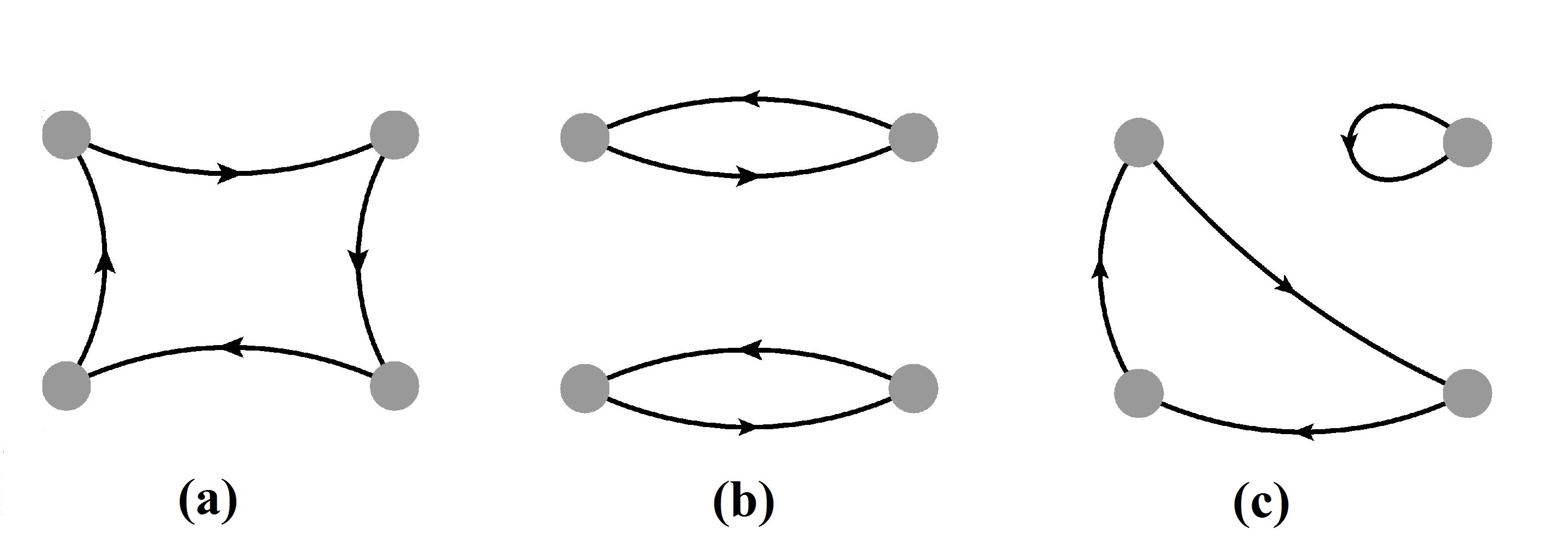
Figure 1: Three independent quark contraction diagrams in $\pi\pi$ scattering up to $\mathcal{O}\!\left(p^{4}\right)\!\,$. Each grey dot represents a $\bar{q}q$ state of definite flavor.

It is not difficult to see that the simplest PQQCD that could make a clean separation of these two contraction diagrams will have four types of fermionic quarks due to the existence of four contraction lines. Meanwhile, two ghost quarks have to be included to keep the number of dynamical DOFs to be two, same as in the original SU(2) theory. Therefore, one concludes that the simplest PQQCD relevant to our work is SU$(4|2)$. The two contraction diagrams can be expressed in terms of scattering amplitudes in SU$(4|2)$ PQChPT as

$$T_{1}(s,t,u) \!\!\!= \!\!\!T_{(u\bar{d})(d\bar{j})\rightarrow(u\bar{k})(k\bar{j})}(s,t,u)\,,$$

$$T_{2}(s,t,u) \!\!\!= \!\!\!T_{(u\bar{d})(j\bar{k})\rightarrow(u\bar{d})(j\bar{k})}(s,t,u)\,.$$ (14)

                   

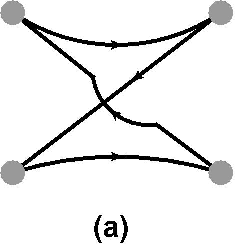
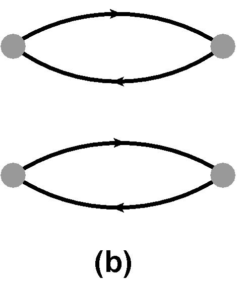
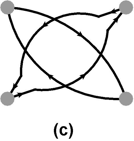
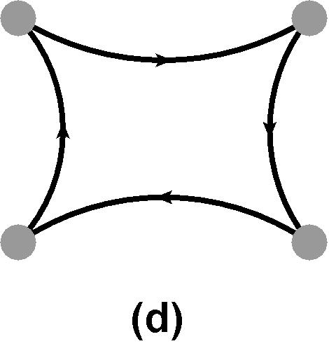
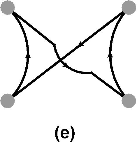
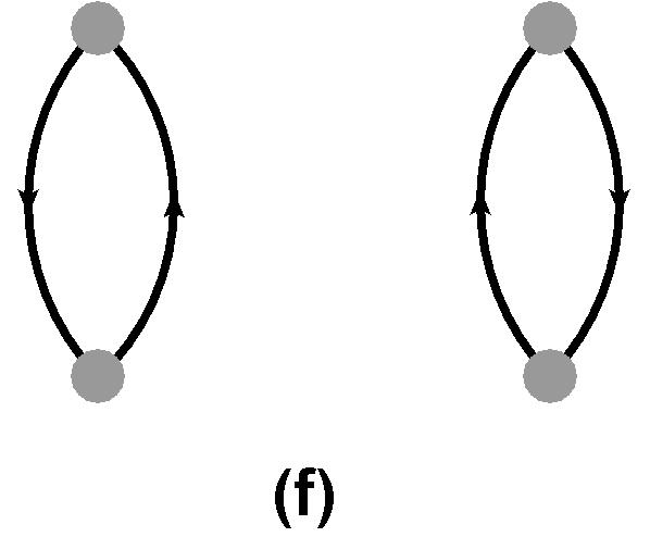
Figure 2: Contraction diagrams with definite type of contractions. Diagram (a) is crossed (C), diagrams (b) and (c) are direct (D), diagrams (d) and (e) are rectangular (R) while diagram (f) is vacuum (V). They correspond to the amplitudes $T_{1}(u,t,s)$, $T_{2}(s,t,u)$, $T_{2}(s,u,t)$, $T_{1}(s,t,u)$, $T_{1}(s,u,t)$ and $T_{2}(t,s,u)$, respectively.

In connection with the lattice calculation, it is instructive to further classify $T_{1}(s,t,u),T_{2}(s,t,u)$ and their crossings into connected, singly-disconnected and doubly-disconnected diagrams, where connected, singly-disconnected and doubly-disconnected diagrams have two, one and zero pair of quark and anti-quark propagating from the initial to the final state, respectively. One sees that $T_{1}(u,t,s),\,T_{2}(s,t,u)$ and $T_{2}(s,u,t)$ are connected diagrams, $T_{1}(s,t,u)$ and $T_{1}(s,u,t)$ are singly-disconnected diagrams while $T_{2}(t,s,u)$ is doubly-disconnected diagram. Adopting the notation of Ref. [4], we name $T_{1}(u,t,s)$ as crossed (C), $T_{2}(s,t,u)$ and $T_{2}(s,u,t)$ as direct (D), $T_{1}(s,t,u)$ and $T_{1}(s,u,t)$ as rectangular (R) and $T_{2}(t,s,u)$ as vacuum (V) diagrams, respectively (see Fig. 2). One can therefore decompose the isospin amplitudes according to the type of contraction of the diagrams as

$$T^{I=0}(s,t,u) \!\!\!= \!\!\!\left[-T_{1}(u,t,s)\right]+\left[T_{2}(s,t,u)+T_{2}(s,u,t)\right]+\left[3\left(T_{1}(s,t,u)+T_{1}(s,u,t)\right)\right]+\left[3T_{2}(t,s,u)\right]$$

$$\equiv T^{I=0}_{C}(s,t,u)\>+\qquad T^{I=0}_{D}(s,t,u)\qquad\>\>\>+\qquad T^{I=0}_{R}(s,t,u)\qquad\qquad\>+T^{I=0}_{V}(s,t,u)\,,$$

$$T^{I=1}(s,t,u) \!\!\!= \!\!\!\left[T_{2}(s,t,u)-T_{2}(s,u,t)\right]+\left[2\left(T_{1}(s,t,u)-T_{1}(s,u,t)\right)\right],$$

$$\equiv \qquad T^{I=1}_{D}(s,t,u)\qquad\>\>\>+\qquad T^{I=1}_{R}(s,t,u)\,,$$

$$T^{I=2}(s,t,u) \!\!\!= \!\!\!\left[2T_{1}(u,t,s)\right]+\left[T_{2}(s,t,u)+T_{2}(s,u,t)\right]$$ (15)

$$\equiv T^{I=2}_{C}(s,t,u)+\qquad T^{I=2}_{D}(s,t,u)\,,$$

where we have defined the individual components $\{T^{I}_{X}(s,t,u)\}$ ($X=D,C,R,V$) for each isospin amplitude $T^{I}(s,t,u)$. One observes that the $I=0$ amplitude has all connected, singly-disconnected and doubly-disconnected pieces, the $I=1$ amplitude has connected and singly-disconnected pieces, while the $I=2$ amplitude has only the connected piece. It is interesting to observe that the doubly-disconnected (V) contribution to the $I=0$ amplitude starts is an NLO effect while the singly-disconnected (R) diagrams are at LO, as was already noticed in Ref. [38]. Therefore, we expect that if the most difficult doubly-disconnected diagram was neglected in a lattice calculation for $I=0$ $\pi\pi$ one would still get results in the correct ball park, while discarding the singly-disconnected diagram would lead to erroneous results. In the case of $I=1$ the singly-disconnected piece actually dominates over the connected piece because the former is of order $\mathcal{O}\!\left(p^{2}\right)\!\,$ while the latter is of order $\mathcal{O}\!\left(p^{4}\right)\!\,$ in chiral power counting.

4 Analytical results

In this section we present the main analytical results of this work. First we define all the special quantities that appear in the loop calculations. The ultraviolet (UV) divergences and chiral logarithms are encoded in:

$$\lambda \!\!\!\equiv \!\!\!-\frac{1}{32\pi^{2}}(\frac{2}{4-d}+\ln 4\pi-\gamma+1)\,,$$

$$\mu_{\pi} \!\!\!\equiv \!\!\!-\frac{M_{\pi}^{2}}{32\pi^{2}F_{\pi}^{2}}\ln\frac{\mu^{2}}{M_{\pi}^{2}}\,.$$ (16)

We also need the Passarino–Veltman two-point function [54]:

$$B_{0}(p^{2},m_{1}^{2},m_{2}^{2})\equiv\frac{(2\pi)^{4-d}}{i\pi^{2}}\int d^{d}k\frac{1}{(k^{2}-m_{1}^{2}+i\varepsilon)((k+p)^{2}-m_{2}^{2}+i\varepsilon)}\,.$$ (17)

Since the only mass that appears in this work is $M_{\pi}$, we may define the function $J_{\pi\pi}$ as

$$J_{\pi\pi}(p^{2})\equiv\frac{1}{16\pi^{2}}B_{0}(p^{2},M_{\pi}^{2},M_{\pi}^{2})\,.$$ (18)

The finite piece in $J_{\pi\pi}(p^{2})$ can be determined by explicitly isolating its infinite piece proportional to $\lambda$

$$J_{\pi\pi}(p^{2})=-2\lambda+J_{\pi\pi}^{r}(p^{2})\,.$$ (19)

Next we shall quote the results for the $\beta$-functions of the $O(p^{4})$ LECs in SU$(4|2)$. Most of them are identical to those in SU(2) because when SU$(4|2)$ is used to calculate processes involving only pions as external legs, it should give an identical result with SU(2). The renormalized LECs are defined through the bare LECs by

$$L_{i}^{\mathrm{PQ}}=L_{i}^{\mathrm{PQ},r}+\lambda\Gamma_{i}\,,$$ (20)

where the $\beta$-function coefficients $\Gamma_{i}$ in SU$(4|2)$ are given in Table 1. One may also define the renormalized physical LECs $\{l_{1}^{r},l_{2}^{r},l_{3}^{r},l_{4}^{r},l_{7}^{r}\}$ through Eq. (11) by replacing $L_{i}^{\mathrm{PQ}}\rightarrow L_{i}^{\mathrm{PQ},r}$. It is also customary to write the physical SU(2) LECs in terms of the scale-independent LECs $\{\bar{l}_{i}\}$ [52],

$$l_{i}^{r}=\gamma_{i}\left(\frac{\bar{l}_{i}}{32\pi^{2}}+\frac{F_{\pi}^{2}}{M_{\pi}^{2}}\mu_{\pi}\right)$$ (21)

for $i=1,...,4$, where $\gamma_{1}=1/3$, $\gamma_{2}=2/3$, $\gamma_{3}=-1/2$ and $\gamma_{4}=2$.

$i$	0	1	2	3	4	5	6	7	8
$\Gamma_{i}$	$\frac{1}{24}$	$\frac{1}{12}$	$\frac{1}{6}$	0	$\frac{1}{8}$	$\frac{1}{4}$	$\frac{3}{32}$	0	0

Table 1: Coefficients of the UV divergence in the SU$(4|2)$ PQChPT.

As a first application and check of the theory, we compute the renormalization of the wave function, mass and decay constant of the pion in SU$(4|2)$. The outcomes are exactly the same as in SU(2) as they should be and are given in [52]

$$Z_{\pi} \!\!\!= \!\!\!1+\frac{4}{3}\mu_{\pi}-\frac{2M_{\pi}^{2}}{F_{\pi}^{2}}l_{4}^{r}-\frac{8M_{\pi}^{2}}{3F_{\pi}^{2}}\lambda\,,$$

$$M_{\pi}^{2} \!\!\!= \!\!\!(M_{\pi}^{2})_{0}\left(1-\frac{M_{\pi}^{2}}{32\pi^{2}F_{\pi}^{2}}\bar{l}_{3}\right),$$

$$F_{\pi} \!\!\!= \!\!\!F_{0}\left(1+\frac{M_{\pi}^{2}}{16\pi^{2}F_{\pi}^{2}}\bar{l}_{4}\right).$$ (22)

Not surprisingly, these expressions depend only on the physical LECs $\{l_{i}^{r}\}$. Further, although these quantities are calculated for pions, they apply equally to all Goldstone bosons made up of only sea or valence quarks, i.e. $\phi_{1},\ldots,\phi_{15}$, due to exact SU(4) symmetry.

The first two contraction diagrams in Fig. 1 can now be computed in SU$(4|2)$. They are

$$T_{1}(s,t,u) \!\!\!= \!\!\!\frac{2M_{\pi}^{2}-u}{2F_{\pi}^{2}}+\left(\frac{3u-4M_{\pi}^{2}}{3F_{\pi}^{2}}\right)\mu_{\pi}+\left(\frac{2M_{\pi}^{4}-4M_{\pi}^{2}(s+t)+s(2s+t)}{12F_{\pi}^{4}}\right)J_{\pi\pi}^{r}(s)$$

$$\!\!\!+\left(\frac{2M_{\pi}^{4}-4M_{\pi}^{2}(s+t)+t(2t+s)}{12F_{\pi}^{4}}\right)J_{\pi\pi}^{r}(t)+\frac{4}{F_{\pi}^{4}}\left(s^{2}+t^{2}+u^{2}-4M_{\pi}^{4}\right)L_{0}^{\mathrm{PQ},r}$$

$$\!\!\!+\frac{2}{F_{\pi}^{4}}\left(4M_{\pi}^{2}u+s^{2}+t^{2}-8M_{\pi}^{4}\right)L_{3}^{\mathrm{PQ},r}-\frac{4M_{\pi}^{2}u}{F_{\pi}^{4}}L_{5}^{\mathrm{PQ},r}+\frac{16M_{\pi}^{4}}{F_{\pi}^{4}}L_{8}^{\mathrm{PQ},r}$$

$$\!\!\!-\frac{M_{\pi}^{4}}{72\pi^{2}F_{\pi}^{4}}+\frac{M_{\pi}^{2}u}{96\pi^{2}F_{\pi}^{4}}+\frac{2u^{2}-s^{2}-t^{2}}{576\pi^{2}F_{\pi}^{4}}\,,$$

$$T_{2}(s,t,u) \!\!\!= \!\!\!\frac{(s-2M_{\pi})^{2}}{4F_{\pi}^{4}}J_{\pi\pi}^{r}(s)+\frac{(u-2M_{\pi})^{2}}{4F_{\pi}^{4}}J_{\pi\pi}^{r}(u)+\left(\frac{2M_{\pi}^{4}+t^{2}}{4F_{\pi}^{4}}\right)J_{\pi\pi}^{r}(t)$$ (23)

$$\!\!\!+\frac{4}{F_{\pi}^{4}}\left(4M_{\pi}^{4}-s^{2}-t^{2}-u^{2}\right)L_{0}^{\mathrm{PQ},r}+\frac{2}{F_{\pi}^{4}}\left(t-2M_{\pi}^{2}\right)^{2}(l_{1}^{r}-2L_{3}^{\mathrm{PQ},r})$$

$$\!\!\!+\frac{1}{F_{\pi}^{4}}\left(s^{2}+u^{2}+4M_{\pi}^{2}t-8M_{\pi}^{4}\right)l_{2}^{r}+\frac{2M_{\pi}^{2}}{F_{\pi}^{4}}\left(t-2M_{\pi}^{2}\right)(l_{4}^{r}-4L_{5}^{\mathrm{PQ},r})$$

$$\!\!\!+\frac{2M_{\pi}^{4}}{F_{\pi}^{4}}(l_{3}^{r}+l_{4}^{r}-8L_{8}^{\mathrm{PQ},r})\,.$$

Each amplitude is finite and scale-independent. One sees that $T_{1}(s,t,u)$ begins at $O(p^{2})$ while $T_{2}(s,t,u)$ begins at $O(p^{4})$ as we expected from counting the number of closed quark loops. Moreover, $T_{1}(s,t,u)$ is symmetric with respect to $s\leftrightarrow t$ while $T_{2}(s,t,u)$ is symmetric with respect to $s\leftrightarrow u$. One also observes that both amplitudes have a dependence on the unphysical LECs, reflecting the fact that the separation of the scattering amplitude into different contraction diagrams is in fact an artificial process. The outcome of this separation is, however, unique because each contraction can be represented by a scattering amplitude in the PQChPT.

As a cross-check, we also computed the $\pi^{+}\pi^{-}\rightarrow\pi^{0}\pi^{0}$ scattering amplitude to $\mathcal{O}\!\left(p^{4}\right)\!\,$ using SU(2) ChPT and confirmed the correctness of Eq. (13). As expected, the dependence on the unphysical LECs drops out as far as the scattering amplitudes of pions are concerned. We also cross-checked Eq. (23) using the formulation briefly discussed in A.

It will be instructive to display numerical results showing the relative importance of different contractions that can be directly contrasted to the lattice results. The main problem, however, is that what is usually displayed in lattice plots are correlation functions $C(t,t^{\prime})=\left\langle\mathcal{O}(t)\mathcal{O}^{\prime\dagger}(t^{\prime})\right\rangle$ of the interpolating field operators $\mathcal{O}$ and $\mathcal{O}^{\prime}$. Such operators are not the $\pi\pi$ field operators in the traditional sense although they have the same quantum numbers, not to say different lattice studies may choose different forms of interpolating operators of their convenience. There is hence no universal matching rule between $C(t,t^{\prime})$ and physical scattering amplitude (on the other hand, carefully constructed ratios between correlation functions may be directly mapped to amplitudes in field theory). With these considerations, we decide to display the partial wave of the isospin amplitudes with a definite type of contraction:

$$T^{IJ}_{X}(s)\equiv\frac{1}{64\pi}\int_{-1}^{+1}T^{I}_{X}\left(s,t(s,\cos\theta),u(s,\cos\theta)\right)P_{J}(\cos\theta)d\cos\theta$$ (24)

where $X$=D,C,R,V denotes the type of contractions while $P_{J}(x)$ is the Legendre polynomial. They have obvious physical meanings and can be easily reconstructed from lattice data. Furthermore, the definition of partial waves does not require the unitarity of the amplitude so it is well-defined for each contraction separately. We shall display both the energy dependence of the partial waves as well as the scattering lengths $a_{X}^{IJ}$ which are given by

$$a_{X}^{IJ}=\lim_{q^{2}\rightarrow 0}\frac{\mathrm{Re}T_{X}^{IJ}(4M_{\pi}^{2}+4q^{2})}{(q^{2})^{J}},$$ (25)

where we have expressed the Mandelstam $s$ around the pion threshold as $s=4(M_{\pi}^{2}+q^{2})$.

Using Eqs. (12) and (23), one is able to compute the contribution to the scattering lengths from each contraction $X$, and the total (i.e. physical) scattering length $a^{IJ}_{\mathrm{tot}}=\sum_{X}a^{IJ}_{X}$. The full results are given in B, and one may readily check the scale independence of each component. The full expressions for $a^{IJ}_{\mathrm{tot}}$ agree with Ref. [52] as long as everything is expressed in terms of physical quantities. All such expressions above are, in principle, concrete predictions of PQChPT that can be directly contrasted with the lattice results. However, the degree of precision for each $a^{IJ}_{X}$ varies depending on the the LECs involved. It is therefore desirable to construct combinations that are least affected by the uncertainties of the LECs. In particular, one may wish to avoid any dependence on the $\bar{l}_{3}$, $L^{\mathrm{PQ,r}}_{0}$ and $L^{\mathrm{PQ,r}}_{3}$ that suffer the most uncertainties in data/lattice fitting (see the discussion in the next section). With such considerations, we find the following combinations (apart from the total scattering length $a^{IJ}_{\mathrm{tot}}$) particularly interesting:

$$a^{00}_{V}-\frac{3}{2}a^{00}_{D} \!\!\!= \!\!\!\frac{M_{\pi}^{4}}{\pi F_{\pi}^{4}}\left[\frac{3\bar{l}_{4}}{64\pi^{2}}-3L^{\mathrm{PQ,r}}_{5}+\frac{9}{512\pi^{2}}+\frac{3F_{\pi}^{2}}{4M_{\pi}^{2}}\mu_{\pi}\right],$$

$$a^{00}_{R}+6a^{00}_{C}-\frac{3M_{\pi}^{2}}{8\pi F_{\pi}^{2}} \!\!\!= \!\!\!\frac{M_{\pi}^{4}}{\pi F_{\pi}^{4}}\left[3L^{\mathrm{PQ,r}}_{5}+\frac{3}{256\pi^{2}}-\frac{3F_{\pi}^{2}}{4M_{\pi}^{2}}\mu_{\pi}\right],$$

$$M_{\pi}^{2}a^{11}_{R}+\frac{8}{3}a^{00}_{C}-30M_{\pi}^{4}a^{02}_{C}-\frac{M_{\pi}^{2}}{8\pi F_{\pi}^{2}} \!\!\!= \!\!\!\frac{M_{\pi}^{4}}{\pi F_{\pi}^{4}}\left[\frac{5L^{\mathrm{PQ,r}}_{5}}{3}-\frac{4L^{\mathrm{PQ,r}}_{8}}{3}-\frac{479}{34560\pi^{2}}-\frac{5F_{\pi}^{2}}{12M_{\pi}^{2}}\mu_{\pi}\right],$$

$$M_{\pi}^{4}a^{02}_{R}-3M_{\pi}^{4}a^{02}_{C}+\frac{4}{5}a^{00}_{C}-\frac{M_{\pi}^{2}}{40\pi F_{\pi}^{2}} \!\!\!= \!\!\!\frac{M_{\pi}^{4}}{\pi F_{\pi}^{4}}\left[\frac{2L^{\mathrm{PQ,r}}_{5}}{5}-\frac{2L^{\mathrm{PQ,r}}_{8}}{5}-\frac{31}{9600\pi^{2}}-\frac{F_{\pi}^{2}}{10M_{\pi}^{2}}\mu_{\pi}\right],$$

$$M_{\pi}^{4}a^{02}_{V}+6M_{\pi}^{4}a^{02}_{C}-\frac{4}{5}a^{00}_{C}+\frac{M_{\pi}^{2}}{40\pi F_{\pi}^{2}} \!\!\!= \!\!\!\frac{M_{\pi}^{4}}{\pi F_{\pi}^{4}}\left[\frac{\bar{l}_{2}}{480\pi^{2}}-\frac{2L^{\mathrm{PQ,r}}_{5}}{5}+\frac{2L^{\mathrm{PQ,r}}_{8}}{5}+\frac{1}{2400\pi^{2}}+\frac{F_{\pi}^{2}}{10M_{\pi}^{2}}\mu_{\pi}\right].$$ (26)

We choose to subtract out all the $\mathcal{O}\!\left(p^{2}\right)\!\,$ contributions in the construction of these combinations above so that none of the contraction diagrams is suppressed by trivial power counting. These relations are useful because they relate the singly- and doubly-disconnected contributions ($a_{R}$ and $a_{V}$) to the connected contributions ($a_{D}$ and $a_{C}$) where the latter can be determined most accurately, and furthermore the uncertainties due to LECs are minimal. They can be used to check the accuracy of lattice studies on the disconnected pieces.

Before ending this section, we shall also present the analytic expressions for the imaginary part of each partial wave in the physical region, i.e. $s\geq 4M_{\pi}^{2}$, as they are LEC-free and are examples of clean PQChPT predictions at one loop. As these are leading order results, they are known to not be very precise. By direct inspection one finds that the only partial waves with a nonvanishing imaginary part are:

$$\mathrm{Im}T^{00}_{D}(s) \!\!\!= \!\!\!\frac{(s-2M_{\pi}^{2})^{2}}{64\pi F_{\pi}^{4}}\mathrm{Im}J^{r}_{\pi\pi}(s)\,,$$

$$\mathrm{Im}T^{00}_{R}(s) \!\!\!= \!\!\!\frac{3(s^{2}-4M_{\pi}^{4})}{128\pi F_{\pi}^{4}}\mathrm{Im}J^{r}_{\pi\pi}(s)\,,$$

$$\mathrm{Im}T^{00}_{V}(s) \!\!\!= \!\!\!\frac{3(s^{2}+2M_{\pi}^{4})}{128\pi F_{\pi}^{4}}\mathrm{Im}J^{r}_{\pi\pi}(s)\,,$$

$$\mathrm{Im}T^{11}_{R}(s) \!\!\!= \!\!\!\frac{(s-4M_{\pi}^{2})^{2}}{576\pi F_{\pi}^{4}}\mathrm{Im}J^{r}_{\pi\pi}(s)\,,$$

$$\mathrm{Im}T^{20}_{D}(s) \!\!\!= \!\!\!\frac{(s-2M_{\pi}^{2})^{2}}{64\pi F_{\pi}^{4}}\mathrm{Im}J^{r}_{\pi\pi}(s)\,,$$ (27)

where

$$\mathrm{Im}J^{r}_{\pi\pi}(s)=\Theta(s-4M_{\pi}^{2})\frac{1}{16\pi}\sqrt{\frac{s-4M_{\pi}^{2}}{s}}\,.$$ (28)

It is also worthwhile to mention that the physical $\pi\pi$ partial waves with definite isospin satisfy the single-channel perturbative unitarity relation:

$$\mathrm{Im}T_{\mathrm{NLO}}^{IJ}(s)=\frac{2|\vec{p}\,|}{\sqrt{s}}\left|T_{\mathrm{LO}}^{IJ}(s)\right|^{2},$$ (29)

where $|\vec{p}|$ is the center-of-mass momentum, but the components from a specific contraction in general do not satisfy such a relation because they do not have definite isospin. Instead, since they can be written as scattering amplitudes in PQChPT, they should satisfy a general multi-channel perturbative unitarity relation:

$$\mathrm{Im}T^{J}_{\mathrm{NLO},ab\rightarrow cd}(s)=\sum_{e,f}\alpha_{ef}\frac{2|\vec{p}\,|}{\sqrt{s}}T^{J}_{\mathrm{LO},ef\rightarrow cd}(s)T^{J*}_{\mathrm{LO},ab\rightarrow ef}(s),$$ (30)

where $\alpha_{ef}=1(2)$ if $e$ and $f$ are (are not) identical particles.

5 Numerical Results

$\bar{l}_{1}$	$-0.4(6)$
$\bar{l}_{2}$	4.3(1)
$\bar{l}_{3}$	3.0(8)
$\bar{l}_{4}$	4.4(2)
$10^{3}L_{0}^{\mathrm{PQ},r}$	1.0(1.1)
$10^{3}(L_{3}^{\mathrm{PQ},r}+2L_{0}^{\mathrm{PQ},r})$	$-1.56(87)$
$10^{3}L_{5}^{\mathrm{PQ},r}$	0.501(43)
$10^{3}L_{8}^{\mathrm{PQ},r}$	0.581(22)

Table 2: The LECs relevant to our work. Values of $\{\bar{l}_{i}\}$ are taken from Refs. [55, 56]. $\{L^{\mathrm{PQ,r}}_{5},L^{\mathrm{PQ,r}}_{8}\}$ and $\{L^{\mathrm{PQ,r}}_{0},L^{\mathrm{PQ,r}}_{3}\}$ are obtained from the NLO and NNLO fits to lattice data, respectively, in Ref. [57] at $\mu=1$ GeV (see the discussion in the text).

In this section we present our numerical results. For this purpose we need the values for both the physical LECs $\bar{l}_{i}$ as well as the unphysical ones $\{L_{i}^{\mathrm{PQ},r}\}$ ($i=0,3,5,8$). $\bar{l}_{1}$, $\bar{l}_{2}$ and $\bar{l}_{4}$ were obtained by sophisticated analysis of the $\pi\pi$ scattering data [55]. $\bar{l}_{3}$ has a very large uncertainty that is, to some extent, reduced by the inclusion of lattice results [56]. For the physical LECs, we quote the values from Ref. [56] that combines fits to data and lattice results, expressed in terms of the scale-independent LECs. For the unphysical LECs, we quote the recent lattice results by the RBC-UKQCD Collaboration from $N_{f}=2+1$ domain wall QCD [57], fitted to the pion mass and decay constant calculated at NLO and next-to-next-to-leading order (NNLO) PQChPT including the NLO finite volume corrections. The underlying principle is that one is free to vary the sea and valence quark masses independently on the lattice, and the outcome of such a manipulation can be matched to PQChPT with non-degenerate Goldstone particles. For $L^{\mathrm{PQ,r}}_{5}$ and $L^{\mathrm{PQ,r}}_{8}$, we take their values from the NLO fit that was performed with satisfactory precision. On the other hand, $L^{\mathrm{PQ,r}}_{0}$ and $L^{\mathrm{PQ,r}}_{3}$ can only be obtained from an NNLO fit (because they do not appear in the NLO mass and decay constant correction) so that their precisions from fitting are less satisfactory. We choose the renormalization scale at $\mu=1$ GeV and pick the data with a 450 MeV mass cut on the unitary pion because the resuls with this cut seem to reproduce the experimental values of $\bar{l}_{i}$ a bit better. We summarize our numerical choice of the LECs in Table 2.

	$10^{2}a_{X}^{00}$	$10^{2}a_{X}^{20}$	$10^{2}M_{\pi}^{2}a_{X}^{11}$	$10^{4}M_{\pi}^{4}a_{X}^{02}$	$10^{4}M_{\pi}^{4}a_{X}^{22}$
D	$0.35\pm 0.24$	$0.35\pm 0.24$	$0.02\pm 0.26$	$3.5\pm 2.0$	$3.5\pm 2.0$
C	$2.41\pm 0.12$	$-4.81\pm 0.23$	0	$0.95\pm 0.96$	$-1.9\pm 1.9$
R	$14.8\pm 0.7$	0	$3.59\pm 0.26$	$6.7\pm 7.8$	0
V	$2.48\pm 0.38$	0	0	$0.8\pm 7.3$	0
Total	$20.0\pm 0.2$	$-4.46\pm 0.07$	$3.61\pm 0.04$	$11.9\pm 0.8$	$1.54\pm 0.71$

Table 3: PQChPT predictions of the scattering lengths from each contraction.

The PQChPT predictions of the scattering lengths $a^{IJ}_{X}$ are given in Table 3. We include only the uncertainties of the LECs from Table 2 in our error analysis and compute the final uncertainties using a simple error propagation formula where the errors of the LECs are assumed to be uncorrelated and are combined in a quadrature. One sees that the uncertainty of each entry is quite large due to the existence of the badly determined LECs $\bar{l}_{3}$, $L^{\mathrm{PQ,r}}_{0}$ and $L^{\mathrm{PQ,r}}_{3}$. On the other hand, the precision of the combinations given in Eq. (26) is much higher:

$$a^{00}_{V}-\frac{3}{2}a^{00}_{D} \!\!\!= \!\!\!(1.96\pm 0.16)\times 10^{-2}$$

$$a^{00}_{R}+6a^{00}_{C}-\frac{3M_{\pi}^{2}}{8\pi F_{\pi}^{2}} \!\!\!= \!\!\!(2.00\pm 0.02)\times 10^{-2}\,,$$

$$M_{\pi}^{2}a^{11}_{R}+\frac{8}{3}a^{00}_{C}-30M_{\pi}^{4}a^{02}_{C}-\frac{M_{\pi}^{2}}{8\pi F_{\pi}^{2}} \!\!\!= \!\!\!(6.38\pm 0.13)\times 10^{-3}\,,$$

$$M_{\pi}^{4}a^{02}_{R}-3M_{\pi}^{4}a^{02}_{C}+\frac{4}{5}a^{00}_{C}-\frac{M_{\pi}^{2}}{40\pi F_{\pi}^{2}} \!\!\!= \!\!\!(1.47\pm 0.03)\times 10^{-3}\,,$$

$$M_{\pi}^{4}a^{02}_{V}+6M_{\pi}^{4}a^{02}_{C}-\frac{4}{5}a^{00}_{C}+\frac{M_{\pi}^{2}}{40\pi F_{\pi}^{2}} \!\!\!= \!\!\!(-4.39\pm 0.47)\times 10^{-4}\,.$$ (31)

One observes that their absolute uncertainties are much smaller than those of $a_{V}^{00}$, $a_{R}^{00}$, $M_{\pi}^{2}a_{R}^{11}$, $M_{\pi}^{4}a_{R}^{02}$ and $M_{\pi}^{4}a_{V}^{02}$ themselves, respectively. We would like to stress that this in fact a nice example of the mutually beneficial interplay between EFT-based theoretical studies and lattice QCD. On the one hand, Eq. (31) serves as a useful check on the degree of accuracy of lattice studies in the handling of the singly- and doubly-disconnected contributions. On the other hand, since the connected diagrams can be calculated easily, they can be used to perform NLO fits for the poorly-known unphysical LECs $L^{\mathrm{PQ,r}}_{0}$ and $L^{\mathrm{PQ,r}}_{3}$ through $a^{IJ}_{D}$ and $a^{IJ}_{C}$ with the formulas given in B, which cannot be done by the fitting to the pion mass and decay constant at NLO. This may greatly reduce the uncertainties in such LECs, which will provide a more precise calculation of quantities in PQChPT at $\mathcal{O}\!\left(p^{4}\right)\!\,$ including the disconnected contributions to $\pi\pi$ scattering.

It will be also instructive to study, instead of just the threshold parameters, the full $s$-dependence of the partial wave amplitudes. Unfortunately, for this case there is no simple combination that allows us to get rid of the uncertainties brought up by $\bar{l}_{3}$, $L^{\mathrm{PQ,r}}_{0}$ and $L^{\mathrm{PQ,r}}_{3}$ that in general grow with increasing $s$. Therefore, we choose to present only the imaginary part of the partial waves because they are LEC-free, as described in the previous section. The plots are given in Fig. 3. One observes that the imaginary part of the $I=0$ amplitude in the physical region comes from the direct, rectangular and vacuum diagrams, while the imaginary part of $I=1(2)$ amplitude in the physical region only originates from rectangular (direct) diagrams.

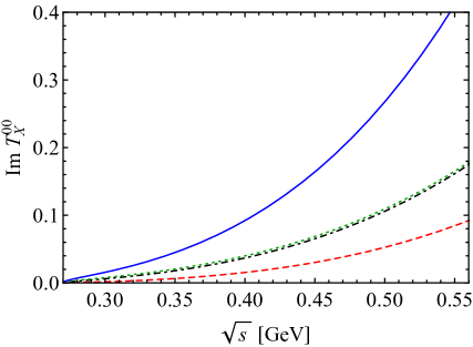
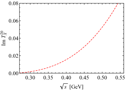
Figure 3: (Color online) Imaginary part of the direct (red dashed), rectangular (black dash-dotted), vacuum (green dotted) and total (blue solid, for $T^{00}$ only) contribution to the partial wave amplitude.

Before ending this section, we would like to point out that if the scattering lengths for the topologically decomposed contractions, defined in Eq. (25), can be extracted from lattice directly, this could hint at a new direction to combine the theoretical and simulation efforts to find a more economical way to calculate the quantities involving disconnected contractions. Assuming that this is feasible, one may extract the the badly known unphysical LECs $L_{0}^{\text{PQ},r}$ and $L_{3}^{\text{PQ},r}$ (see Table 2) from calculating the easier $D$- and $C$-type contractions, and feed them back into the formulae collected in B, or Eqs. (26) and (31), to get the more difficult contractions.

6 Summary

Isoscalar pion-pion scattering has been and still is a formidable challenge in lattice calculations mainly due to the existence of doubly-disconnected/vacuum Wick contractions which are extremely noisy. In this work we have studied the contributions from different types of quark contractions to the pion-pion scattering amplitudes by means of SU$(4|2)$ PQChPT up to $\mathcal{O}\!\left(p^{4}\right)\!\,$. By suitably choosing the quark content of the incoming and outgoing Goldstone particles, one is able to probe the scattering amplitudes with any given contraction. We express the direct, crossed, rectangular and vacuum contraction diagrams in terms of two independent amplitudes $T_{1}(s,t,u)$, $T_{2}(s,t,u)$ and their crossings. In order to provide definite predictions, we derived the analytic expressions for $J=0,1,2$ scattering lengths resulting from definite contractions. On top of that, we constructed observables that are minimally affected by the uncertainties of the low-energy constants in PQChPT, including specific combinations of scattering lengths and the imaginary part of partial wave amplitudes.

Our work is a nice example of a mutually-beneficial interplay between effective field theory and lattice QCD. The ability of lattice QCD to isolate diagrams of different contractions enables NLO fitting of certain unphysical LECs in PQChPT, and hence greatly improves its predictive power. In particular, we have given expressions in terms of these LECs for various scattering lengths decomposed into different types of contractions. They can be used to extract the values of the unphysical LECs in PQChPT. It would also be great if lattice calculations could decompose the results of scattering lengths into different contractions so that the results from PQChPT and lattice QCD can be cross-checked. In this sense, our prediction may even serve as a measure of the accuracy level of lattice calculation of quark disconnected diagrams.

There are lots of other hadronic quantities whose calculation in lattice involves the expensive and noisy disconnected diagrams, such as the $\pi K$ and $K\bar{K}$ scattering processes, the parity-odd pion-nucleon coupling and so on. The same kind of interplay could be useful in the study of them. The necessary PQChPT analysis will be done in future works.

Acknowledgements

We are grateful to Xu Feng and Liuming Liu for helpful discussions and to Xu Feng for a careful reading and valuable comments on the first version of this manuscript. We also thank the referee for very useful comments. FKG acknowledges the warm hospitality of the INPAC, CYS acknowledges the warm hospitality of the ITP of CAS, and UGM acknowledges warm hospitality of the IHEP of CAS and ITP of CAS, where part of this work was done. This work is supported in part by NSFC and DFG through funds provided to the Sino-German CRC 110 “Symmetries and the Emergence of Structure in QCD” (NSFC Grant No. 11621131001, DFG Grant No. TRR110), by NSFC (Grant No. 11575110, No. 11175115 and No. 11647601), by the Thousand Talents Plan for Young Professionals, by the CAS Key Research Program of Frontier Sciences (Grant No. QYZDB-SSW-SYS013), by the CAS President’s International Fellowship Initiative (PIFI) (Grant No. 2017VMA0025), and by the Natural Science Foundation of Shanghai under Grant No. 15DZ2272100 and No. 15ZR1423100.

Appendix A PQChPT by integrating out $\Phi_{0}$

For practical purposes, sometimes it is convenient to use a method different from the one used in the main text to implement the constraint of $\mathrm{Str}(\Phi)=0$. This can be achieved by adding to the LO Lagrangian in Eq. (8) a mass term for the singlet field $\Phi_{0}\equiv\mathrm{Str}(\Phi)/\sqrt{2}$, $-m_{0}^{2}\Phi_{0}^{2}$ [42], which is later on integrated out by setting $m_{0}$ to infinity. In this formalism, the matrix $U$ is written as $U=\exp{\left(i\sqrt{2}\Phi/F_{0}\right)}$, with

$$\Phi=\begin{pmatrix}\phi&\chi^{\dagger}\\ \chi&\tilde{\phi}\end{pmatrix},\quad\phi=\begin{pmatrix}\eta_{u}&\pi^{+}&\phi_{u\bar{j}}&\phi_{u\bar{k}}\\ \pi^{-}&\eta_{d}&\phi_{d\bar{j}}&\phi_{d\bar{k}}\\ \phi_{j\bar{u}}&\phi_{j\bar{d}}&\eta_{j}&\phi_{j\bar{k}}\\ \phi_{k\bar{u}}&\phi_{k\bar{d}}&\phi_{k\bar{j}}&\eta_{k}\end{pmatrix},\quad\tilde{\phi}=\begin{pmatrix}\eta_{\tilde{j}}&\phi_{\tilde{j}\bar{\tilde{k}}}\\ \phi_{\tilde{k}\bar{\tilde{j}}}&\eta_{\tilde{k}}\end{pmatrix},\quad\chi=\begin{pmatrix}\phi_{\tilde{j}\bar{u}}&\phi_{\tilde{j}\bar{d}}&\phi_{\tilde{j}\bar{j}}&\phi_{\tilde{j}\bar{k}}\\ \phi_{\tilde{k}\bar{u}}&\phi_{\tilde{k}\bar{d}}&\phi_{\tilde{k}\bar{j}}&\phi_{\tilde{k}\bar{k}}\end{pmatrix},$$ (32)

where the diagonal elements $\eta_{q}$’s are neutral states made of $q\bar{q}$. After integrating our the singlet component $\Phi_{0}$, one gets the propagators of these neutral states. For the case of SU$(4|2)$ with all quarks and ghost quarks degenerate, they are rather simple:

$$G^{ab}(k^{2})=\frac{i}{k^{2}-(M_{\pi}^{2})_{0}+i\varepsilon}\left(\delta^{ab}\epsilon^{a}-\frac{1}{2}\right),$$ (33)

where $\epsilon^{a}=+1(-1)$ for neutral particles that are made out of fermionic (bosonic) quark-antiquark pairs. The propagators for all other mesons take the normal form except for an additional factor of $-1$ for states made of a pair of ghost quark and anti-quark.

Appendix B Scattering Lengths

In this appendix we present the analytic expressions for the $J=0,1,2$ scattering lengths resulting from each contraction $X$ as well as the physical scattering length $a^{IJ}_{\mathrm{tot}}$.

$I=0,J=0$:

$$a^{00}_{D} \!\!\!= \!\!\!-\frac{M_{\pi}^{2}}{8\pi F_{\pi}^{2}}\left[\mu_{\pi}+\frac{M_{\pi}^{2}}{F_{\pi}^{2}}\left(-\frac{\bar{l}_{1}}{24\pi^{2}}-\frac{\bar{l}_{2}}{12\pi^{2}}+\frac{\bar{l}_{3}}{64\pi^{2}}+\frac{\bar{l}_{4}}{16\pi^{2}}+24L^{\mathrm{PQ,r}}_{0}+8L^{\mathrm{PQ,r}}_{3}-8L^{\mathrm{PQ,r}}_{5}\right.\right.$$

$$\left.\left.+8L^{\mathrm{PQ,r}}_{8}+\frac{1}{64\pi^{2}}\right)\right],$$

$$a_{C}^{00} \!\!\!= \!\!\!\frac{M_{\pi}^{2}}{32\pi F_{\pi}^{2}}\left[1-2\mu_{\pi}+\frac{M_{\pi}^{2}}{F_{\pi}^{2}}\left(-48L^{\mathrm{PQ,r}}_{0}-16L^{\mathrm{PQ,r}}_{3}+16L^{\mathrm{PQ,r}}_{5}-16L^{\mathrm{PQ,r}}_{8}-\frac{1}{16\pi^{2}}\right)\right],$$

$$a_{R}^{00} \!\!\!= \!\!\!\frac{3M_{\pi}^{2}}{16\pi F_{\pi}^{2}}\left[1-2\mu_{\pi}+\frac{M_{\pi}^{2}}{F_{\pi}^{2}}\left(48L^{\mathrm{PQ,r}}_{0}+16L^{\mathrm{PQ,r}}_{3}+16L^{\mathrm{PQ,r}}_{8}+\frac{1}{8\pi^{2}}\right)\right],$$

$$a^{00}_{V} \!\!\!= \!\!\!\frac{9M_{\pi}^{2}}{16\pi F_{\pi}^{2}}\left[\mu_{\pi}+\frac{M_{\pi}^{2}}{F_{\pi}^{2}}\left(\frac{\bar{l}_{1}}{72\pi^{2}}+\frac{\bar{l}_{2}}{36\pi^{2}}-\frac{\bar{l}_{3}}{192\pi^{2}}+\frac{\bar{l}_{4}}{16\pi^{2}}-8L^{\mathrm{PQ,r}}_{0}-\frac{8L^{\mathrm{PQ,r}}_{3}}{3}-\frac{8L^{\mathrm{PQ,r}}_{5}}{3}\right.\right.$$

$$\left.\left.-\frac{8L^{\mathrm{PQ,r}}_{8}}{3}+\frac{5}{192\pi^{2}}\right)\right],$$

$$a^{00}_{\mathrm{tot}} \!\!\!= \!\!\!\frac{7M_{\pi}^{2}}{32\pi F_{\pi}^{2}}\left[1+\frac{M_{\pi}^{2}}{\pi^{2}F_{\pi}^{2}}\left(\frac{5\bar{l}_{1}}{84}+\frac{5\bar{l}_{2}}{42}-\frac{5\bar{l}_{3}}{224}+\frac{\bar{l}_{4}}{8}+\frac{5}{32}\right)\right];$$ (34)

$I=2,J=0$:

$$a^{20}_{D} \!\!\!= \!\!\!a^{00}_{D}\,,$$

$$a^{20}_{C} \!\!\!= \!\!\!-2a^{00}_{C}\,,$$

$$a^{20}_{\mathrm{tot}} \!\!\!= \!\!\!-\frac{M_{\pi}^{2}}{16\pi F_{\pi}^{2}}\left[1+\frac{M_{\pi}^{2}}{\pi^{2}F_{\pi}^{2}}\left(-\frac{\bar{l}_{1}}{12}-\frac{\bar{l}_{2}}{6}+\frac{\bar{l}_{3}}{32}+\frac{\bar{l}_{4}}{8}-\frac{1}{32}\right)\right];$$ (35)

$I=1,J=1$:

$$a^{11}_{D} \!\!\!= \!\!\!\frac{1}{12\pi F_{\pi}^{2}}\left[\mu_{\pi}+\frac{M_{\pi}^{2}}{F_{\pi}^{2}}\left(-\frac{\bar{l}_{1}}{24\pi^{2}}+\frac{\bar{l}_{2}}{24\pi^{2}}+\frac{\bar{l}_{4}}{16\pi^{2}}+8L^{\mathrm{PQ,r}}_{3}-4L^{\mathrm{PQ,r}}_{5}-\frac{13}{384\pi^{2}}\right)\right],$$

$$a^{11}_{R} \!\!\!= \!\!\!\frac{1}{24\pi F_{\pi}^{2}}\left[1-2\mu_{\pi}+\frac{M_{\pi}^{2}}{F_{\pi}^{2}}\left(-16L^{\mathrm{PQ,r}}_{3}+8L^{\mathrm{PQ,r}}_{5}-\frac{13}{288\pi^{2}}\right)\right],$$

$$a^{11}_{\mathrm{tot}} \!\!\!= \!\!\!\frac{1}{24\pi F_{\pi}^{2}}\left[1+\frac{M_{\pi}^{2}}{\pi^{2}F_{\pi}^{2}}\left(-\frac{\bar{l}_{1}}{12}+\frac{\bar{l}_{2}}{12}+\frac{\bar{l}_{4}}{8}-\frac{65}{576}\right)\right];$$ (36)

$I=0,J=2$:

$$a^{02}_{D} \!\!\!= \!\!\!\frac{1}{90\pi F_{\pi}^{4}}\left[\frac{F_{\pi}^{2}}{M_{\pi}^{2}}\mu_{\pi}+\frac{\bar{l}_{1}}{16\pi^{2}}+\frac{\bar{l}_{2}}{16\pi^{2}}-24\pi^{2}L^{\mathrm{PQ,r}}_{0}-12\pi^{2}L^{\mathrm{PQ,r}}_{3}-\frac{77}{640\pi^{2}}\right],$$

$$a^{02}_{C} \!\!\!= \!\!\!\frac{1}{180\pi F_{\pi}^{4}}\left[\frac{F_{\pi}^{2}}{M_{\pi}^{2}}\mu_{\pi}-24\pi^{2}L^{\mathrm{PQ,r}}_{0}-12\pi^{2}L^{\mathrm{PQ,r}}_{3}+\frac{13}{320\pi^{2}}\right],$$

$$a^{02}_{R} \!\!\!= \!\!\!\frac{1}{30\pi F_{\pi}^{4}}\left[-\frac{F_{\pi}^{2}}{M_{\pi}^{2}}\mu_{\pi}+24L^{\mathrm{PQ,r}}_{0}+6L^{\mathrm{PQ,r}}_{3}-\frac{57}{1920\pi^{2}}\right],$$

$$a^{02}_{V} \!\!\!= \!\!\!\frac{1}{60\pi F_{\pi}^{4}}\left[\frac{F_{\pi}^{2}}{M_{\pi}^{2}}\mu_{\pi}+\frac{\bar{l}_{2}}{8\pi^{2}}-24L^{\mathrm{PQ,r}}_{0}-\frac{3}{20\pi^{2}}\right],$$

$$a^{02}_{\mathrm{tot}} \!\!\!= \!\!\!\frac{1}{1440\pi^{3}F_{\pi}^{4}}\left[\bar{l}_{1}+4\bar{l}_{2}-\frac{53}{8}\right];$$ (37)

$I=2,J=2$:

$$a^{22}_{D} \!\!\!= \!\!\!a^{02}_{D}\,,$$

$$a^{22}_{C} \!\!\!= \!\!\!-2a^{02}_{C}\,,$$

$$a^{22}_{\mathrm{tot}} \!\!\!= \!\!\!\frac{1}{1440\pi^{3}F_{\pi}^{4}}\left[\bar{l}_{1}+\bar{l}_{2}-\frac{103}{40}\right].$$ (38)

References

- [1] J. Bijnens, G. Colangelo, G. Ecker, J. Gasser, M. E. Sainio, Elastic pi pi scattering to two loops, Phys. Lett. B374 (1996) 210–216. arXiv:hep-ph/9511397, doi:10.1016/0370-2693(96)00165-7.
- [2] B. Ananthanarayan, G. Colangelo, J. Gasser, H. Leutwyler, Roy equation analysis of pi pi scattering, Phys. Rept. 353 (2001) 207–279. arXiv:hep-ph/0005297, doi:10.1016/S0370-1573(01)00009-6.
- [3] R. Garcia-Martin, R. Kaminski, J. R. Peláez, J. Ruiz de Elvira, F. J. Yndurain, The Pion-pion scattering amplitude. IV: Improved analysis with once subtracted Roy-like equations up to 1100 MeV, Phys. Rev. D83 (2011) 074004. arXiv:1102.2183, doi:10.1103/PhysRevD.83.074004.
- [4] Y. Kuramashi, M. Fukugita, H. Mino, M. Okawa, A. Ukawa, Lattice QCD calculation of full pion scattering lengths, Phys. Rev. Lett. 71 (1993) 2387–2390. doi:10.1103/PhysRevLett.71.2387.
- [5] M. Fukugita, Y. Kuramashi, M. Okawa, H. Mino, A. Ukawa, Hadron scattering lengths in lattice QCD, Phys. Rev. D52 (1995) 3003–3023. arXiv:hep-lat/9501024, doi:10.1103/PhysRevD.52.3003.
- [6] X. Li, et al., Anisotropic lattice calculation of pion scattering using an asymmetric box, JHEP 06 (2007) 053. arXiv:hep-lat/0703015, doi:10.1088/1126-6708/2007/06/053.
- [7] S. R. Sharpe, R. Gupta, G. W. Kilcup, Lattice calculation of I = 2 pion scattering length, Nucl. Phys. B383 (1992) 309–354. doi:10.1016/0550-3213(92)90681-Z.
- [8] R. Gupta, A. Patel, S. R. Sharpe, I = 2 pion scattering amplitude with Wilson fermions, Phys. Rev. D48 (1993) 388–396. arXiv:hep-lat/9301016, doi:10.1103/PhysRevD.48.388.
- [9] S. Aoki, et al., I=2 pion scattering length with the Wilson fermion, Phys. Rev. D66 (2002) 077501. arXiv:hep-lat/0206011, doi:10.1103/PhysRevD.66.077501.
- [10] X. Du, G.-w. Meng, C. Miao, C. Liu, I = 2 pion scattering length with improved actions on anisotropic lattices, Int. J. Mod. Phys. A19 (2004) 5609–5614. arXiv:hep-lat/0404017, doi:10.1142/S0217751X04019573.
- [11] J.-W. Chen, D. O’Connell, R. S. Van de Water, A. Walker-Loud, Ginsparg-Wilson pions scattering on a staggered sea, Phys. Rev. D73 (2006) 074510. arXiv:hep-lat/0510024, doi:10.1103/PhysRevD.73.074510.
- [12] S. R. Beane, T. C. Luu, K. Orginos, A. Parreno, M. J. Savage, A. Torok, A. Walker-Loud, Precise Determination of the I=2 pi pi Scattering Length from Mixed-Action Lattice QCD, Phys. Rev. D77 (2008) 014505. arXiv:0706.3026, doi:10.1103/PhysRevD.77.014505.
- [13] X. Feng, K. Jansen, D. B. Renner, The pi+ pi+ scattering length from maximally twisted mass lattice QCD, Phys. Lett. B684 (2010) 268–274. arXiv:0909.3255, doi:10.1016/j.physletb.2010.01.018.
- [14] J. J. Dudek, R. G. Edwards, M. J. Peardon, D. G. Richards, C. E. Thomas, The phase-shift of isospin-2 pi-pi scattering from lattice QCD, Phys. Rev. D83 (2011) 071504. arXiv:1011.6352, doi:10.1103/PhysRevD.83.071504.
- [15] S. R. Beane, E. Chang, W. Detmold, H. W. Lin, T. C. Luu, K. Orginos, A. Parreno, M. J. Savage, A. Torok, A. Walker-Loud, The I=2 pipi S-wave Scattering Phase Shift from Lattice QCD, Phys. Rev. D85 (2012) 034505. arXiv:1107.5023, doi:10.1103/PhysRevD.85.034505.
- [16] J. J. Dudek, R. G. Edwards, C. E. Thomas, S and D-wave phase shifts in isospin-2 pi pi scattering from lattice QCD, Phys. Rev. D86 (2012) 034031. arXiv:1203.6041, doi:10.1103/PhysRevD.86.034031.
- [17] C. Helmes, C. Jost, B. Knippschild, C. Liu, J. Liu, L. Liu, C. Urbach, M. Ueding, Z. Wang, M. Werner, Hadron-hadron interactions from Nf = 2 + 1 + 1 lattice QCD: isospin-2 scattering length, JHEP 09 (2015) 109. arXiv:1506.00408, doi:10.1007/JHEP09(2015)109.
- [18] S. Aoki, et al., Lattice QCD Calculation of the rho Meson Decay Width, Phys. Rev. D76 (2007) 094506. arXiv:0708.3705, doi:10.1103/PhysRevD.76.094506.
- [19] X. Feng, K. Jansen, D. B. Renner, Resonance Parameters of the rho-Meson from Lattice QCD, Phys. Rev. D83 (2011) 094505. arXiv:1011.5288, doi:10.1103/PhysRevD.83.094505.
- [20] C. B. Lang, D. Mohler, S. Prelovsek, M. Vidmar, Coupled channel analysis of the rho meson decay in lattice QCD, Phys. Rev. D84 (5) (2011) 054503, [Erratum: Phys. Rev.D89,no.5,059903(2014)]. arXiv:1105.5636, doi:10.1103/PhysRevD.89.059903,10.1103/PhysRevD.84.054503.
- [21] S. Aoki, et al., Meson Decay in 2+1 Flavor Lattice QCD, Phys. Rev. D84 (2011) 094505. arXiv:1106.5365, doi:10.1103/PhysRevD.84.094505.
- [22] C. Pelissier, A. Alexandru, Resonance parameters of the rho-meson from asymmetrical lattices, Phys. Rev. D87 (1) (2013) 014503. arXiv:1211.0092, doi:10.1103/PhysRevD.87.014503.
- [23] J. J. Dudek, R. G. Edwards, C. E. Thomas, Energy dependence of the resonance in elastic scattering from lattice QCD, Phys. Rev. D87 (3) (2013) 034505, [Erratum: Phys. Rev.D90,no.9,099902(2014)]. arXiv:1212.0830, doi:10.1103/PhysRevD.87.034505,10.1103/PhysRevD.90.099902.
- [24] D. J. Wilson, R. A. Briceño, J. J. Dudek, R. G. Edwards, C. E. Thomas, Coupled scattering in -wave and the resonance from lattice QCD, Phys. Rev. D92 (9) (2015) 094502. arXiv:1507.02599, doi:10.1103/PhysRevD.92.094502.
- [25] X. Feng, S. Aoki, S. Hashimoto, T. Kaneko, Timelike pion form factor in lattice QCD, Phys. Rev. D91 (5) (2015) 054504. arXiv:1412.6319, doi:10.1103/PhysRevD.91.054504.
- [26] G. S. Bali, S. Collins, A. Cox, G. Donald, M. Göckeler, C. B. Lang, A. Schäfer, and resonances on the lattice at nearly physical quark masses and , Phys. Rev. D93 (5) (2016) 054509. arXiv:1512.08678, doi:10.1103/PhysRevD.93.054509.
- [27] J. Bulava, B. Fahy, B. Hörz, K. J. Juge, C. Morningstar, C. H. Wong, and scattering phase shifts from lattice QCD, Nucl. Phys. B910 (2016) 842–867. arXiv:1604.05593, doi:10.1016/j.nuclphysb.2016.07.024.
- [28] D. Guo, A. Alexandru, R. Molina, M. Döring, Rho resonance parameters from lattice QCD, Phys. Rev. D94 (3) (2016) 034501. arXiv:1605.03993, doi:10.1103/PhysRevD.94.034501.
- [29] C. Alexandrou, L. Leskovec, S. Meinel, J. Negele, S. Paul, M. Petschlies, A. Pochinsky, G. Rendon, S. Syritsyn, -wave scattering and the resonance from lattice QCDarXiv:1704.05439.
- [30] Z. Fu, Lattice QCD study of the s-wave scattering lengths in the I=0 and 2 channels, Phys. Rev. D87 (7) (2013) 074501. arXiv:1303.0517, doi:10.1103/PhysRevD.87.074501.
- [31] R. A. Briceño, J. J. Dudek, R. G. Edwards, D. J. Wilson, Isoscalar scattering and the meson resonance from QCD, Phys. Rev. Lett. 118 (2) (2017) 022002. arXiv:1607.05900, doi:10.1103/PhysRevLett.118.022002.
- [32] L. Liu, et al., Isospin-0 s-wave scattering length from twisted mass lattice QCDarXiv:1612.02061.
- [33] Z. Bai, et al., Standard Model Prediction for Direct CP Violation in Decay, Phys. Rev. Lett. 115 (21) (2015) 212001. arXiv:1505.07863, doi:10.1103/PhysRevLett.115.212001.
- [34] H. Neff, N. Eicker, T. Lippert, J. W. Negele, K. Schilling, On the low fermionic eigenmode dominance in QCD on the lattice, Phys. Rev. D64 (2001) 114509. arXiv:hep-lat/0106016, doi:10.1103/PhysRevD.64.114509.
- [35] J. Foley, K. Jimmy Juge, A. O’Cais, M. Peardon, S. M. Ryan, J.-I. Skullerud, Practical all-to-all propagators for lattice QCD, Comput. Phys. Commun. 172 (2005) 145–162. arXiv:hep-lat/0505023, doi:10.1016/j.cpc.2005.06.008.
- [36] M. Peardon, J. Bulava, J. Foley, C. Morningstar, J. Dudek, R. G. Edwards, B. Joo, H.-W. Lin, D. G. Richards, K. J. Juge, A Novel quark-field creation operator construction for hadronic physics in lattice QCD, Phys. Rev. D80 (2009) 054506. arXiv:0905.2160, doi:10.1103/PhysRevD.80.054506.
- [37] J. Wasem, Lattice QCD Calculation of Nuclear Parity Violation, Phys. Rev. C85 (2012) 022501. arXiv:1108.1151, doi:10.1103/PhysRevC.85.022501.
- [38] F.-K. Guo, L. Liu, U.-G. Meißner, P. Wang, Tetraquarks, hadronic molecules, meson-meson scattering and disconnected contributions in lattice QCD, Phys. Rev. D88 (2013) 074506. arXiv:1308.2545, doi:10.1103/PhysRevD.88.074506.
- [39] C. W. Bernard, M. F. L. Golterman, Partially quenched gauge theories and an application to staggered fermions, Phys. Rev. D49 (1994) 486–494. arXiv:hep-lat/9306005, doi:10.1103/PhysRevD.49.486.
- [40] S. R. Sharpe, N. Shoresh, Partially quenched QCD with nondegenerate dynamical quarks, Nucl. Phys. Proc. Suppl. 83 (2000) 968–970. arXiv:hep-lat/9909090, doi:10.1016/S0920-5632(00)91860-7.
- [41] S. R. Sharpe, N. Shoresh, Physical results from unphysical simulations, Phys. Rev. D62 (2000) 094503. arXiv:hep-lat/0006017, doi:10.1103/PhysRevD.62.094503.
- [42] S. R. Sharpe, N. Shoresh, Partially quenched chiral perturbation theory without Phi0, Phys. Rev. D64 (2001) 114510. arXiv:hep-lat/0108003, doi:10.1103/PhysRevD.64.114510.
- [43] C. Bernard, M. Golterman, On the foundations of partially quenched chiral perturbation theory, Phys. Rev. D88 (1) (2013) 014004. arXiv:1304.1948, doi:10.1103/PhysRevD.88.014004.
- [44] S. Sharpe, Applications of Chiral Perturbation theory to lattice QCD, in: Workshop on Perspectives in Lattice QCD Nara, Japan, October 31-November 11, 2005, 2006. arXiv:hep-lat/0607016.
-
[45]
M. Golterman,
Applications
of chiral perturbation theory to lattice QCD, in: Modern perspectives in
lattice QCD: Quantum field theory and high performance computing.
Proceedings, International School, 93rd Session, Les Houches, France, August
3-28, 2009, 2009, pp. 423–515.
arXiv:0912.4042.
URL http://inspirehep.net/record/840837/files/arXiv:0912.4042.pdf - [46] P. H. Damgaard, Partially quenched chiral condensates from the replica method, Phys. Lett. B476 (2000) 465–470. arXiv:hep-lat/0001002, doi:10.1016/S0370-2693(00)00154-4.
- [47] P. H. Damgaard, K. Splittorff, Partially quenched chiral perturbation theory and the replica method, Phys. Rev. D62 (2000) 054509. arXiv:hep-lat/0003017, doi:10.1103/PhysRevD.62.054509.
- [48] M. Della Morte, A. Jüttner, Quark disconnected diagrams in chiral perturbation theory, JHEP 11 (2010) 154. arXiv:1009.3783, doi:10.1007/JHEP11(2010)154.
- [49] A. Jüttner, Revisiting the pion’s scalar form factor in chiral perturbation theory, JHEP 01 (2012) 007. arXiv:1110.4859, doi:10.1007/JHEP01(2012)007.
- [50] L. Giusti, M. Lüscher, Chiral symmetry breaking and the Banks-Casher relation in lattice QCD with Wilson quarks, JHEP 03 (2009) 013. arXiv:0812.3638, doi:10.1088/1126-6708/2009/03/013.
- [51] J. Gasser, H. Leutwyler, Chiral Perturbation Theory: Expansions in the Mass of the Strange Quark, Nucl. Phys. B250 (1985) 465–516. doi:10.1016/0550-3213(85)90492-4.
- [52] J. Gasser, H. Leutwyler, Chiral Perturbation Theory to One Loop, Annals Phys. 158 (1984) 142. doi:10.1016/0003-4916(84)90242-2.
- [53] J. L. Petersen, Meson-meson scattering, Phys. Rept. 2 (1971) 155–252. doi:10.1016/0370-1573(71)90014-7.
- [54] G. Passarino, M. J. G. Veltman, One Loop Corrections for e+ e- Annihilation Into mu+ mu- in the Weinberg Model, Nucl. Phys. B160 (1979) 151–207. doi:10.1016/0550-3213(79)90234-7.
- [55] G. Colangelo, J. Gasser, H. Leutwyler, scattering, Nucl. Phys. B603 (2001) 125–179. arXiv:hep-ph/0103088, doi:10.1016/S0550-3213(01)00147-X.
- [56] J. Bijnens, G. Ecker, Mesonic low-energy constants, Ann. Rev. Nucl. Part. Sci. 64 (2014) 149–174. arXiv:1405.6488, doi:10.1146/annurev-nucl-102313-025528.
- [57] P. A. Boyle, et al., Low energy constants of SU(2) partially quenched chiral perturbation theory from Nf=2+1 domain wall QCD, Phys. Rev. D93 (5) (2016) 054502. arXiv:1511.01950, doi:10.1103/PhysRevD.93.054502.