Decoupled field integral equations for electromagnetic scattering from homogeneous penetrable obstacles

Abstract

We present a new method for the analysis of electromagnetic scattering from homogeneous penetrable bodies. Our approach is based on a reformulation of the governing Maxwell equations in terms of two uncoupled vector Helmholtz systems: one for the electric field and one for the magnetic field. This permits the derivation of resonance-free Fredholm equations of the second kind that are stable at all frequencies, insensitive to the genus of the scatterers, and invertible for all passive materials including those with negative permittivities or permeabilities. We refer to these as decoupled field integral equations.

1 Introduction

A standard problem in electromagnetics concerns the solution of of the Maxwell equations in an exterior domain, when an incoming wave is scattered by a collection of bounded penetrable obstacles. There is a vast literature on integral equation methods for such problems, with standard formulations for the piecewise constant case described, for example, in the papers [10, 15, 16, 17, 20]. Boundary integral methods are natural in the homogeneous (piecewise constant) setting, since they require only the discretization of the inclusion boundaries rather than the domain, satisfy the Silver-Müller radiation condition exactly, and can be coupled with suitable fast algorithms, such as the fast multipole method (FMM).

Working in the frequency domain and assuming a time dependence of the form $e^{-i\omega t}$, Maxwell’s equations in a linear, isotropic material are given by

$$\nabla\times{\bf H}^{tot} =-i\omega\epsilon_{L}\,{\bf E}^{tot},$$ (1)

$$\nabla\times{\bf E}^{tot} =i\omega\mu_{L}{\bf H}^{tot},$$

where $\epsilon_{L}$ and $\mu_{L}$ are the local permittivity and permeability of the medium, respectively. Here, ${\bf E}^{tot}$ and ${\bf H}^{tot}$ denote the total electric and magnetic fields which we express in the form

$${\bf E}^{tot}={\bf E}^{in}+{\bf E}_{0},\quad{\bf H}^{tot}={\bf H}^{in}+{\bf H}_{0},$$ (2)

in the exterior region and

$${\bf E}^{tot}={\bf E},\quad{\bf H}^{tot}={\bf H},$$ (3)

within the inclusions. Here, $\{{\bf E}^{in},{\bf H}^{in}\}$ is a known incoming electromagnetic field.

For the sake of simplicity, we will assume that the penetrable obstacles are all made of the same material and that they define a compactly supported open region $D$ in $\mathbb{R}^{3}$ whose boundary, denoted by $\partial D$, consists of a finite number of disjoint, closed surfaces belonging to class $C^{2}$. We also assume that the exterior region $\mathbb{R}^{3}/\overline{D}$ is connected. We will denote by $\epsilon_{0},\mu_{0}$ the material properties of the exterior domain and by $\epsilon,\mu$ the material properties of the inclusions.

At obstacle boundaries, the Maxwell equations (1) must satisfy the continuity conditions [12, 19]:

$${\bf n}\times({\bf E}_{0}-{\bf E}) =-{\bf n}\times{\bf E}^{in}$$ (4)

$${\bf n}\times({\bf H}_{0}-{\bf H}) =-{\bf n}\times{\bf H}^{in},$$

where ${\bf n}$ denotes the outward normal vector to the interface.

Definition 1.

The boundary value problem defined by (1) with $\{\epsilon_{L},\mu_{L}\}=\{\epsilon,\mu\}$ inside the inclusions and $\{\epsilon_{L},\mu_{L}\}=\{\epsilon_{0},\mu_{0}\}$ in the exterior domain, together with the interface conditions (4), will be referred to as the Maxwell transmission problem.

It is well-known that, under mild assumptions on the permittivity and permeability [6, 17], the Maxwell transmission problem has a unique solution, so long as the scattered field satisfied the Silver-Müller radiation condition:

$$\begin{array}[]{ll}\sqrt{\frac{\mu_{0}}{\epsilon_{0}}}{\bf H}_{0}(\boldsymbol{x})\times\frac{\boldsymbol{x}}{|\boldsymbol{x}|}-{\bf E}_{0}(\boldsymbol{x})=o\Big{(}\frac{1}{|\boldsymbol{x}|}\Big{)},&|\boldsymbol{x}|\rightarrow\infty\,.\end{array}$$ (5)

We will restrict our attention in this paper to the case $\omega\geq 0$ with $\epsilon_{0},\mu_{0}>0$ and

$$\Im{(\epsilon)} >0\text{ or }\epsilon\in\mathbb{R}^{+}$$ (6)

$$\Im{(\mu)} >0\text{ or }\mu\in\mathbb{R}^{+},$$

where $\mathbb{R}^{+}$ denotes the positive real numbers. For the sake of completeness, we provide a simple proof of uniqueness for this parameter regime (Appendix A), which includes all metamaterials wth non-zero dissipation.

The standard approach to the development of integral equation methods is based on the classical vector and scalar potentials [19]: We let

$$\boldsymbol{A}_{0}(\boldsymbol{x})=\mu_{0}S_{k_{0}}[\boldsymbol{J}_{0}](\boldsymbol{x}),\ \ \boldsymbol{A}(\boldsymbol{x})=\mu S_{k}[\boldsymbol{J}](\boldsymbol{x}),$$

where

$$S_{k}[\boldsymbol{J}](\boldsymbol{x})\equiv\int_{\partial D}g_{k}(\boldsymbol{x}-\boldsymbol{y})\,\boldsymbol{J}(\boldsymbol{y})\,ds_{\boldsymbol{y}}\,,$$ (7)

$g_{k}(\boldsymbol{x})=e^{ik|\boldsymbol{x}\|}/\|\boldsymbol{x}\|$, $k=\sqrt{w^{2}\epsilon\mu}$, and $k_{0}=\sqrt{w^{2}\epsilon_{0}\mu_{0}}$, Here, $\boldsymbol{J},\boldsymbol{J}_{0}$ can be viewed as surface electric currents. When the argument of the square root is complex, $k$ is taken to lie in the upper half-plane. We define the vector anti-potentials by

$${\tilde{\boldsymbol{A}}}_{0}(\boldsymbol{x})=\epsilon_{0}S_{k_{0}}[\boldsymbol{K}_{0}](\boldsymbol{x}),\ \ {\tilde{\boldsymbol{A}}}(\boldsymbol{x})=\epsilon S_{k}[\boldsymbol{K}](\boldsymbol{x}),$$

where $\boldsymbol{K},\boldsymbol{K}_{0}$ can be viewed as surface magnetic currents. The scalar potentials and antipotentials are given by

$$\phi_{0}(\boldsymbol{x})=\frac{1}{i\omega\epsilon_{0}\mu_{0}}\nabla\cdot\boldsymbol{A}_{0},\ \ \phi(\boldsymbol{x})=\frac{1}{i\omega\epsilon\mu}\nabla\cdot\boldsymbol{A},$$

and

$$\psi_{0}(\boldsymbol{x})=\frac{1}{i\omega\epsilon_{0}\mu_{0}}\nabla\cdot{\tilde{\boldsymbol{A}}}_{0},\ \ \psi(\boldsymbol{x})=\frac{1}{i\omega\epsilon\mu}\nabla\cdot{\tilde{\boldsymbol{A}}}.$$

From these, we may write

$${\bf E}_{0} =i\omega\boldsymbol{A}_{0}-\nabla\phi_{0}-\frac{1}{\epsilon_{0}}\nabla\times{\tilde{\boldsymbol{A}}}_{0},$$ (8)

$${\bf H}_{0} =\frac{1}{\mu_{0}}\nabla\times\boldsymbol{A}_{0}+i\omega{\tilde{\boldsymbol{A}}}_{0}-\nabla\psi_{0}$$

for $\boldsymbol{x}$ in the exterior, and

$${\bf E} =i\omega\boldsymbol{A}-\nabla\phi-\frac{1}{\epsilon}\nabla\times{\tilde{\boldsymbol{A}}},$$ (9)

$${\bf H} =\frac{1}{\mu}\nabla\times\boldsymbol{A}+i\omega{\tilde{\boldsymbol{A}}}-\nabla\psi$$

for $\boldsymbol{x}$ inside the inclusions.

The number of degrees of freedom in the representation is reduced by assuming that the tangential vector fields $\boldsymbol{J}_{0},\boldsymbol{J},\boldsymbol{K}_{0},\boldsymbol{K}$ satisfy

$$\boldsymbol{J}^{s}:=\epsilon_{0}\boldsymbol{J}_{0}=\epsilon\boldsymbol{J}\qquad\boldsymbol{K}^{s}:=\mu_{0}\boldsymbol{K}_{0}=\mu\boldsymbol{K}\,.$$ (10)

Imposing the conditions (4) and using the relations (14) yields Müller’s integral equation [17] for $\boldsymbol{J}^{s},\boldsymbol{K}^{s}$:

$$-\boldsymbol{n}\times{\bf E}^{\operatorname{inc}}=-\left(\frac{\mu_{0}+\mu}{2}\right)\boldsymbol{K}^{s}-\left(\mu_{0}\nabla\times S_{k_{0}}-\mu\nabla\times S_{k}\right)[\boldsymbol{K}^{s}]+i\omega\left(\epsilon_{0}\mu_{0}S_{k_{0}}-\epsilon\mu S_{k}\right)[\boldsymbol{J}^{s}]$$

$$-\frac{1}{i\omega}\left(\nabla\nabla\cdot S_{k_{0}}-\nabla\nabla\cdot S_{k}\right)[\boldsymbol{J}^{s}]$$

$$-\boldsymbol{n}\times{\bf H}^{\operatorname{inc}}=\left(\frac{\epsilon_{0}+\epsilon}{2}\right)\boldsymbol{J}^{s}+\left(\epsilon_{0}\nabla\times S_{k_{0}}-\epsilon\nabla\times S_{k}\right)[\boldsymbol{J}^{s}]+i\omega\left(\epsilon_{0}\mu_{0}S_{k_{0}}-\epsilon\mu S_{k}\right)[\boldsymbol{K}^{s}]$$

$$-\frac{1}{i\omega}\left(\nabla\nabla\cdot S_{k_{0}}-\nabla\nabla\cdot S_{k}\right)[\boldsymbol{K}^{s}]$$

In Müller’s original formulation, the unknowns are actually the tangential components of ${\bf E}$ and ${\bf H}$ rather than fictitious currents, and the integral equation above is the dual of the formulation in [17]. We refer the reader to [3, 4, 5, 6, 9, 18, 31] for further details.

It suffices, for our present purposes, to note that all of the operators appearing above turn out to be compact and that Müller’s integral equation is a resonance-free Fredholm equation of the second kind. It is uniquely solvable for the passive materials under consideration here. Moreover, it can be shown that the integral equation is stable even in the low-frequency regime. Unfortunately, the representation itself is subject to “low-frequency breakdown”. That is, once the currents are known, the evalution of ${\bf E}$ or ${\bf H}$ from (8), (9) is unstable as $\omega\rightarrow 0$, because of catastrophic cancellation in the scalar potentials.

Rather than writing the scalar potentials and antipotentials as above, however, we may write

$$\phi_{0}(\boldsymbol{x})=S_{k_{0}}[\rho](\boldsymbol{x})\ \ \phi(\boldsymbol{x})=S_{k}[\rho](\boldsymbol{x}),$$ (11)

and

$$\psi_{0}(\boldsymbol{x})=S_{k_{0}}[\rho_{M}](\boldsymbol{x}),\ \ \psi(\boldsymbol{x})=S_{k}[\rho_{M}](\boldsymbol{x}),$$ (12)

where

$$S_{k}[\rho](\boldsymbol{x})\equiv\int_{\partial D}g_{k}(\boldsymbol{x}-\boldsymbol{y})\,\rho(\boldsymbol{y})\,ds_{\boldsymbol{y}}\,,$$ (13)

and

$$\rho=\nabla_{S}\cdot\boldsymbol{J}/(i\omega),\quad\rho_{M}=\nabla_{S}\cdot\boldsymbol{K}/(i\omega).$$ (14)

Here, $\nabla_{S}$ denotes the surface divergence operator.

Remark 1.

The problem of low-frequency breakdown lies in the computation of $\rho,\rho_{M}$. Since ill-conditioning occurs even for a fixed $\omega$ under mesh refinement, a more descriptive term is, perhaps, dense-mesh breakdown [24], which we will use interchangeably.

One mechanism to overcome dense-mesh breakdown is to solve two auxiliary integral equations for the scalar potentials [26], using the representation (8) and (9) and imposing the two interface conditions

$$\boldsymbol{n}\cdot(\epsilon_{0}{\bf E}^{tot}_{0}-\epsilon{\bf E}^{tot})=0,$$

$$\frac{\nabla\cdot{\bf E}_{0}}{k_{0}^{2}}-\frac{\nabla\cdot{\bf E}}{k^{2}}=0.$$

The first is a standard condition for dielectric interfaces and leads to the scalar equation

$$\epsilon_{0}\frac{\partial\phi_{0}}{\partial n}-\epsilon\frac{\partial\phi}{\partial n}=f$$ (15)

where

$$f=\boldsymbol{n}\cdot{\bf E}^{in}+i\omega\boldsymbol{n}\cdot(\epsilon_{0}^{2}\mu_{0}\cdot S_{k_{0}}[\boldsymbol{J}_{0}]-\epsilon^{2}\mu\cdot S_{k}[\boldsymbol{J}])+\boldsymbol{n}\cdot\nabla\times(\epsilon\mu S_{k}[\boldsymbol{K}]-\epsilon_{0}\mu_{0}S_{k_{0}}[\boldsymbol{K}_{0}])$$

The second interface condition follows from the fact that ${\bf E}$ and ${\bf E}_{0}$ are divergence-free, with the particular linear combination chosen to yield the equation

$$\phi_{0}-\phi=\frac{\nabla\cdot S_{k}[\boldsymbol{J}]-\nabla\cdot S_{k_{0}}[\boldsymbol{J}_{0}]}{i\omega}.$$ (16)

Similarly, one can derive the two scalar equations for $\psi$ and $\psi_{0}$:

$$\mu_{0}\frac{\partial\psi_{0}}{\partial n}-\mu\frac{\partial\psi}{\partial n}=g$$ (17)

where

$$g=\boldsymbol{n}\cdot{\bf H}^{in}+i\omega\boldsymbol{n}\cdot(\mu_{0}^{2}\epsilon_{0}\cdot S_{k_{0}}[\boldsymbol{K}_{0}]-\mu^{2}\epsilon\cdot S_{k}[\boldsymbol{K}])+\boldsymbol{n}\cdot\nabla\times(\epsilon\mu S_{k}[\boldsymbol{J}]-\epsilon_{0}\mu_{0}S_{k_{0}}[\boldsymbol{J}_{0}]),$$

and

$$\psi_{0}-\psi=\frac{\nabla\cdot S_{k}[\boldsymbol{K}]-\nabla\cdot S_{k_{0}}[\boldsymbol{K}_{0}]}{i\omega}.$$ (18)

Without entering into details, it is well-known that the interface problems (15),(16) and (17),(18) are uniquely solvable without dense-mesh breakdown using a Fredholm equation of the second kind [29, 21]. (Care must be taken in computing the right-hand sides for (16) and (18). In particular, catastrophic cancellation can be avoided for small $\omega$ by computing the difference asymptotically.)

Remark 2.

A solver for the Maxwell transmission problem based on first solving the Müller integral equation, followed by solving the systems (15),(16) and (17),(18) will be referred to as a decoupled charge-current formulation. It yields stable solutions for real $\epsilon,\mu$ [26], but can have resonances for lossy materials.

It is also worth noting that alternative “charge-current” formulations have been developed [8, 22, 23, 32] that make use of electric and magnetic charge as additional, distinct unknowns. Using the representation (8), (9) with $\boldsymbol{A},\boldsymbol{A}_{0},{\tilde{\boldsymbol{A}}},{\tilde{\boldsymbol{A}}}_{0}$ defined in terms of the unknowns $\boldsymbol{J},\boldsymbol{K}$ and the relation (10), with $\phi,\phi_{0},\psi,\psi_{0}$ defined in terms of $\rho,\rho_{M}$, one can seek to enforce

$${\bf n}\cdot(\epsilon_{0}{\bf E}_{0}-\epsilon{\bf E}) =-{\bf n}\cdot\,\epsilon_{0}{\bf E}^{in}$$ (19)

$${\bf n}\cdot(\mu_{0}{\bf H}_{0}-\mu{\bf H}) =-{\bf n}\cdot\mu_{0}{\bf H}^{in},$$

$${\bf n}\times({\bf E}_{0}-{\bf E}) =-{\bf n}\times{\bf E}^{in}$$

$${\bf n}\times({\bf H}_{0}-{\bf H}) =-{\bf n}\times{\bf H}^{in}.$$

This avoids low-frequency breakdown and leads to a Fredholm equation of the second kind. However, these methods are subject to spurious “near resonances.” The precise location of these resonances depends on the specific charge-current scheme employed, the material properties and the geometry, illustrated in Fig. 1 below. A “decoupled potential formulation,” presented in [1], extends the method of [25] for perfect conductors to the dielectric case. It, too, is subject to spurious resonances when the real parts of $\epsilon$ and $\mu$ are not both positive, because of the existence of “transmission” eigenvalues [14].

In [7], an integral representation was developed using four scalar densities supported on the obstacle boundaries. This “generalized Debye source” representation yields a resonance-free Fredholm integral equations of the second kind, valid for all the material properties of interest in the present paper. The topology of the domain, however, plays a critical role and the method requires a basis for surface harmonic vector fields. Finally, there is a substantial literature on “single source” integral equations, which involve only one unknown tangential vector field (see, for example [10, 15, 30]). Unfortunately, the original single source formulations typically do not lead to Fredholm equations, involve hypersingular operators, and/or are subject to low-frequency breakdown. Significant progress, however, has been made in formulating equations that are immune from low-frequency breakdown (see, for example, [2, 16, 24]). Unfortunately, none of these equations have been shown to be resonance-free for the full range of passive materials which we consider here.

In the present paper, we describe a new system of decoupled Fredholm integral equations for the electric and magnetic fields that are resonance-free for all problems of interest, insensitive to the genus of the scatterer, and immune from low-frequency breakdown.

2 Generalized transmission problems

Our approach to the Maxwell transmission problem is based on the analysis of two nonstandard boundary value problems governed by the vector Helmholtz equation. More precisely, we introduce the electric and magnetic transmission problems as follows:

Definition 2.

By the vector electric transmission problem we mean the calculation of a vector field

$$\begin{array}[]{ll}{\bf E}\in C^{2}(D)\cap C(\overline{D})&\mbox{for $\boldsymbol{x}\in D$};\\ {\bf E}_{0}\in C^{2}(\mathbb{R}^{3}\setminus\overline{D})\cap C(\mathbb{R}^{3}/D)&\mbox{for $\boldsymbol{x}\in\mathbb{R}^{3}\setminus\overline{D}$},\end{array}$$

with

$$\Delta{\bf E}+k^{2}{\bf E} =0, \quad\boldsymbol{x} \in D$$ (20)

$$\Delta{\bf E}_{0}+k_{0}^{2}{\bf E}_{0} =0, \quad\boldsymbol{x} \in\mathbb{R}^{3}/\overline{D}$$

that satisfies the interface conditions

$$\boldsymbol{n}\times\big{(}{\bf E}_{0}-{\bf E}\big{)}=\mathbf{f}\\$$ (21)

$$\boldsymbol{n}\times\left(\frac{\nabla\times{\bf E}_{0}}{\mu_{0}}-\frac{\nabla\times{\bf E}}{\mu}\right)=\mathbf{g}$$ (22)

$$\nabla\cdot{\bf E}_{0}-\nabla\cdot{\bf E}=q$$ (23)

$$\boldsymbol{n}\cdot\left(\epsilon_{0}{\bf E}_{0}-\epsilon{\bf E}\right)=p$$ (24)

and the radiation condition

$$\begin{array}[]{ll}\nabla\times{\bf E}_{0}(\boldsymbol{x})\times\frac{\boldsymbol{x}}{|\boldsymbol{x}|}+\frac{\boldsymbol{x}}{|\boldsymbol{x}|}\nabla\cdot{\bf E}_{0}(\boldsymbol{x})-ik_{0}{\bf E}_{0}(\boldsymbol{x})=o\Big{(}\frac{1}{|\boldsymbol{x}|}\Big{)},&|\boldsymbol{x}|\rightarrow\infty\,,\end{array}$$ (25)

where $\mathbf{f}\in C^{0,\alpha}_{t}(Div,\partial D)$, $\mathbf{g}\in C^{0,\alpha}_{t}(\partial D)$ and $q,p\in C^{0,\alpha}(\partial D)$.

Definition 3.

By the vector magnetic transmission problem we mean the calculation of a vector field

$$\begin{array}[]{ll}{\bf H}\in C^{2}(D)\cap C(\overline{D})&\mbox{for $\boldsymbol{x}\in D$};\\ {\bf H}_{0}\in C^{2}(\mathbb{R}^{3}\setminus\overline{D})\cap C(\mathbb{R}^{3}/D)&\mbox{for $\boldsymbol{x}\in\mathbb{R}^{3}\setminus\overline{D}$},\end{array}$$

with

$$\Delta{\bf H}+k^{2}{\bf H} =0, \quad\boldsymbol{x} \in D$$ (26)

$$\Delta{\bf H}_{0}+k_{0}^{2}{\bf H}_{0} =0, \quad\boldsymbol{x} \in\mathbb{R}^{3}/\overline{D}$$

that satisfies the interface conditions

$$\boldsymbol{n}\times\left({\bf H}_{0}-{\bf H}\right)=\mathbf{f}^{\prime}$$ (27)

$$\boldsymbol{n}\times\left(\frac{\nabla\times{\bf H}_{0}}{\epsilon_{0}}-\frac{\nabla\times{\bf H}}{\epsilon}\right)=\mathbf{g}^{\prime}$$ (28)

$$\nabla\cdot{\bf H}_{0}-\nabla\cdot{\bf H}=q^{\prime}$$ (29)

$$\boldsymbol{n}\cdot\left(\mu_{0}{\bf H}_{0}-\mu{\bf H}\right)=p^{\prime}$$ (30)

and the radiation condition

$$\begin{array}[]{ll}\nabla\times{\bf H}_{0}(\boldsymbol{x})\times\frac{\boldsymbol{x}}{|\boldsymbol{x}|}+\frac{\boldsymbol{x}}{|\boldsymbol{x}|}\nabla\cdot{\bf H}_{0}(\boldsymbol{x})-ik{\bf H}_{0}(\boldsymbol{x})=o\Big{(}\frac{1}{|\boldsymbol{x}|}\Big{)},&|\boldsymbol{x}|\rightarrow\infty\,,\end{array}$$ (31)

where $\mathbf{f}^{\prime}\in C^{0,\alpha}_{t}(Div,\partial D)$, $\mathbf{g}^{\prime}\in C^{0,\alpha}_{t}(\partial D)$ and $q^{\prime},p^{\prime}\in C^{0,\alpha}(\partial D)$.

Theorem 1.

The vector electric and magnetic transmission problems have unique solutions for $\omega\geq 0$.

Proof.

See Appendix C. ∎

Definition 4.

The layer potentials in (7) and (13) are referred to as single layer potentials, with vector or scalar densities, $\boldsymbol{J}$ and $\rho$, respectively. Letting $\boldsymbol{x}^{\prime}$ denote a point on $\partial D$, they are continuous across the interface. Their normal derivatives, denoted by $S_{k}^{\prime}$, satisfy the jump conditions [3, 4]:

$$\lim_{{\boldsymbol{x}\rightarrow\boldsymbol{x}^{\prime}}^{\pm}}\boldsymbol{n}(\boldsymbol{x}^{\prime})\cdot\nabla S_{k}[\boldsymbol{J}](\boldsymbol{x})=\pm\frac{1}{2}\boldsymbol{J}(\boldsymbol{x}^{\prime})+S_{k}^{\prime}[\boldsymbol{J}](\boldsymbol{x}^{\prime})$$ (32)

$$\lim_{{\boldsymbol{x}\rightarrow\boldsymbol{x}^{\prime}}^{\pm}}\boldsymbol{n}(\boldsymbol{x}^{\prime})\cdot\nabla S_{k}[\rho](\boldsymbol{x})=\pm\frac{1}{2}\rho(\boldsymbol{x}^{\prime})+S_{k}^{\prime}[\rho](\boldsymbol{x}^{\prime})$$ (33)

where $S_{k}^{\prime}[\boldsymbol{J}](\boldsymbol{x}^{\prime})$ and $S_{k}^{\prime}[\rho](\boldsymbol{x}^{\prime})$ are defined in the principal value sense, $\lim_{{\boldsymbol{x}\rightarrow\boldsymbol{x}^{\prime}}^{-}}$ denotes the interior limit ($\boldsymbol{x}\in D$) and $\lim_{{\boldsymbol{x}\rightarrow\boldsymbol{x}^{\prime}}^{+}}$ denotes the exterior limit ($\boldsymbol{x}\in\mathbb{R}^{3}/\overline{D}$).

The double layer potential is defined by

$$D_{k}[\rho](\boldsymbol{x})\equiv\int_{\partial D}\nabla g_{k}(\boldsymbol{x}-\boldsymbol{y})\cdot\boldsymbol{n}(\boldsymbol{y})\,\rho(\boldsymbol{y})\,ds_{\boldsymbol{y}}\,.$$ (34)

It is well-known to satisfy the jump condition

$$\lim_{{\boldsymbol{x}\rightarrow\boldsymbol{x}^{\prime}}^{\pm}}D_{k}[\rho](\boldsymbol{x})=\mp\frac{1}{2}\rho(\boldsymbol{x}^{\prime})+D_{k}[\rho](\boldsymbol{x}^{\prime})$$

where $D_{k}[\rho](\boldsymbol{x}^{\prime})$ is defined in the principal value sense. Finally, we let $M_{k}$ denote the operator obtained by taking the limit:

$$\lim_{{\boldsymbol{x}\rightarrow\boldsymbol{x}^{\prime}}^{\pm}}\boldsymbol{n}(\boldsymbol{x}^{\prime})\times\nabla\times S_{k}[\boldsymbol{J}](\boldsymbol{x})\equiv\mp\boldsymbol{J}(\boldsymbol{x}^{\prime})+M_{k}[\boldsymbol{J}](\boldsymbol{x}^{\prime})\,,$$ (35)

where $M_{k}[\boldsymbol{J}](\boldsymbol{x}^{\prime})$ is defined in the principal value sense.

Theorem 2.

Let

$${\bf E}_{0} =\mu_{0}\nabla\times S_{k_{0}}[\boldsymbol{a}]-\mu_{0}S_{k_{0}}[\boldsymbol{n}\sigma]+\mu_{0}\epsilon_{0}S_{k_{0}}[\boldsymbol{b}]+\nabla S_{k_{0}}[\rho] \boldsymbol{x}\in\mathbb{R}^{3}/\overline{D}$$ (36)

$${\bf E} =\mu\nabla\times S_{k}[\boldsymbol{a}]-\mu S_{k}[\boldsymbol{n}\sigma]+\mu\epsilon S_{k}[\boldsymbol{b}]+\nabla S_{k}[\rho] \boldsymbol{x}\in D\,.$$

Imposing the conditions (21) - (24) yields the second kind Fredholm equation

$$\frac{\mu_{0}+\mu}{2}\boldsymbol{a}+\big{(}\mu_{0}M_{k_{0}}-\mu M_{k}\big{)}[\boldsymbol{a}]-\boldsymbol{n}\times\big{(}\mu_{0}S_{k_{0}}-\mu S_{k}\big{)}[\boldsymbol{n}\sigma]+$$ (37)

$$\boldsymbol{n}\times\big{(}\mu_{0}\epsilon_{0}S_{k_{0}}-\mu\epsilon S_{k}\big{)}[\boldsymbol{b}]+\boldsymbol{n}\times\nabla\big{(}S_{k_{0}}-S_{k}\big{)}[\rho] =\mathbf{f}$$

$$\frac{\mu_{0}+\mu}{2}\sigma+\big{(}\mu_{0}D_{k_{0}}-\mu D_{k}\big{)}[\sigma]+\nabla\cdot\big{(}\mu_{0}\epsilon_{0}S_{k_{0}}-\mu\epsilon S_{k}\big{)}[\boldsymbol{b}]$$

$$-\omega^{2}\big{(}\mu_{0}\epsilon_{0}S_{k_{0}}-\mu\epsilon S_{k}\big{)}[\rho] =q$$

$$\frac{\epsilon_{0}+\epsilon}{2}\boldsymbol{b}+(\epsilon_{0}M_{k_{0}}-\epsilon M_{k})[\boldsymbol{b}]+\boldsymbol{n}\times\nabla\times\nabla\times\big{(}S_{k_{0}}-S_{k}\big{)}[\boldsymbol{a}]-$$

$$\boldsymbol{n}\times\nabla\times\big{(}S_{k_{0}}-S_{k}\big{)}[\boldsymbol{n}\sigma] =\mathbf{g}$$

$$-\frac{\epsilon_{0}+\epsilon}{2}\rho+(\epsilon_{0}S^{\prime}_{k_{0}}-\epsilon S^{\prime}_{k})[\rho]+\boldsymbol{n}\cdot\nabla\times\big{(}\epsilon_{0}\mu_{0}S_{k_{0}}-\epsilon\mu S_{k}\big{)}[\boldsymbol{a}]-$$

$$\boldsymbol{n}\cdot\big{(}\epsilon_{0}\mu_{0}S_{k_{0}}-\epsilon\mu S_{k}\big{)}[\boldsymbol{n}\sigma]+\boldsymbol{n}\cdot\big{(}\mu_{0}\epsilon_{0}^{2}S_{k_{0}}-\mu\epsilon^{2}S_{k}\big{)}[\boldsymbol{b}] =p\,.$$

which is invertible for $(\mathbf{f},p,\mathbf{g},q)$ in the function space

$$C_{t}^{0,\alpha}(Div,\partial D)\times C^{0,\alpha}(\partial D)\times C_{t}^{0,\alpha}(\partial D)\times C^{0,\alpha}(\partial D)$$

, so long as $\epsilon,\mu$ satisfy the conditions (6). Given the solution to (37), the functions given by (36) solve the vector electric transmission problem.

Proof.

See Appendix D. ∎

The analogous result follows trivially for the vector magnetic transmission problem.

Theorem 3.

Let

$${\bf H}_{0} =\epsilon_{0}\nabla\times S_{k_{0}}(\boldsymbol{a})-\epsilon_{0}S_{k_{0}}(\boldsymbol{n}\sigma)+\mu_{0}\epsilon_{0}S_{k_{0}}(\boldsymbol{b})+\nabla S_{k_{0}}(\rho) \boldsymbol{x}\in\mathbb{R}^{3}/\overline{D}$$ (38)

$${\bf H} =\epsilon\nabla\times S_{k}(\boldsymbol{a})-\epsilon S_{k}(\boldsymbol{n}\sigma)+\mu\epsilon S_{k}(\boldsymbol{b})+\nabla S_{k}(\rho) \boldsymbol{x}\in D\,.$$

Imposing the conditions (27) - (30) yields a second kind Fredholm equation, identical to (37) with $\{\epsilon,\mu\}$ and $\{\epsilon_{0},\mu_{0}\}$ interchanged. Given the solution to this dual integral equation, the functions given by (38) solve the vector magnetic transmission problem.

Theorem 4.

Let ${\bf E}^{in},{\bf H}^{in}$ denote an incoming electromagnetic field, let ${\bf E}_{0},{\bf E}$ denote the solution of the vector electric transmission problem with right hand side

$$\mathbf{f} =-\boldsymbol{n}\times{\bf E}^{in}$$ (39)

$$\mathbf{g} =-i\omega\boldsymbol{n}\times{\bf H}^{in}$$

$$q =0$$

$$p =-\boldsymbol{n}\cdot\epsilon_{0}{\bf E}^{in}\,,$$

and let ${\bf H}_{0},{\bf H}$ denote the solution of the vector magnetic transmission problem with right hand side

$$\mathbf{f}^{\prime} =-\boldsymbol{n}\times{\bf H}^{in}$$ (40)

$$\mathbf{g}^{\prime} =-i\omega\boldsymbol{n}\times{\bf E}^{in}$$

$$q^{\prime} =0$$

$$p^{\prime} =-\boldsymbol{n}\cdot\mu_{0}{\bf H}^{in}\,.$$

Then, the fields ${\bf E}_{0},{\bf E},{\bf H}_{0},{\bf H}$ satisfy the Maxwell equations and solve the Maxwell transmission problem.

Proof.

The result follows from Theorem 1 and the fact that the desired scattered fields satisfy the vector electric and magnetic transmission problems by inspection. The boundary data $\mathbf{f},\mathbf{g},q,p$ and $\mathbf{f}^{\prime},\mathbf{g}^{\prime},q^{\prime},p^{\prime}$ satisfy the required regularity conditions assuming that the incoming fields ${\bf E}^{in}$ and ${\bf H}^{in}$ are induced by exterior sources away from $\partial D$. ∎

Theorem 5.

The solution of the vector electric and magnetic transmission problems satisfy the following stability properties uniformly on the interval $\omega\in[0,\omega_{\max}]$.

$$\|{\bf E}_{0}\|_{\alpha,\mathbb{R}^{3}\backslash D}\leq K(\partial D,k_{\max})\Big{(}\|\mathbf{f}\|_{\alpha,\partial D}+\|\mathbf{g}\|_{\alpha,\partial D}+\|q\|_{\alpha,\partial D}+\|p\|_{\alpha,\partial D}\Big{)}$$ (41)

$$\|{\bf H}_{0}\|_{\alpha,\mathbb{R}^{3}\backslash D}\leq K(\partial D,k_{\max})\Big{(}\|\mathbf{f}\|_{\alpha,\partial D}+\|\mathbf{g}\|_{\alpha,\partial D}+\|q\|_{\alpha,\partial D}+\|p\|_{\alpha,\partial D}\Big{)}$$ (42)

For Maxwellian incoming fields, we have

$$\|{\bf E}_{0}\|_{\alpha,\mathbb{R}^{3}\backslash D}\leq K(\partial D,k_{\max})\Big{(}\|{\bf E}^{in}\|_{\alpha,\partial D}+\|{\bf H}^{in}\|_{\alpha,\partial D}\Big{)}$$ (43)

$$\|{\bf H}_{0}\|_{\alpha,\mathbb{R}^{3}\backslash D}\leq K(\partial D,k_{\max})\Big{(}\|{\bf E}^{in}\|_{\alpha,\partial D}+\|{\bf H}^{in}\|_{\alpha,\partial D}\Big{)}.$$ (44)

Proof.

See Appendix E. ∎

As a consequence of the preceding theorems, one can solve the Maxwell transmission problem replacing it with the vector electric and magnetic transmission problems. This permits evaluation of the fields all the way to $\omega=0$ without low frequency breakdown and without regard to the genus of the surface.

3 High Frequency Scaling

While the representation (36) is sufficient for proving existence and uniqueness, it is not well scaled at high frequencies. For the sake of simplicity, we will asume that the scatterer has dimensions on the order of unity, so that $\omega$ itself is a measure of size in terms of wavelength. Following Kress [13] and our earlier work [28], when $\omega>1$, we suggest that the representation for the electromagnetic field be modified as follows:

$${\bf E}_{0} =\mu_{0}\nabla\times S_{k_{0}}(\boldsymbol{a})-\omega\mu_{0}S_{k_{0}}(\boldsymbol{n}\sigma)+\omega\mu_{0}\epsilon_{0}S_{k_{0}}(\boldsymbol{b})+\nabla S_{k_{0}}(\rho) \boldsymbol{x}\in\mathbb{R}^{3}/\overline{D}$$ (45)

$${\bf E} =\mu\nabla\times S_{k}(\boldsymbol{a})-\omega\mu S_{k}(\boldsymbol{n}\sigma)+\omega\mu\epsilon S_{k}(\boldsymbol{b})+\nabla S_{k}(\rho) \boldsymbol{x}\in D$$

We also rescale the jump conditions (21)-(24) as follows:

$$\boldsymbol{n}\times\big{(}{\bf E}_{0}-{\bf E}\big{)}=\mathbf{f}=-\boldsymbol{n}\times{\bf E}^{\operatorname{inc}}\\$$

$$\frac{1}{\omega}\boldsymbol{n}\times\Big{(}\frac{\nabla\times{\bf E}_{0}}{\mu_{0}}-\frac{\nabla\times{\bf E}}{\mu}\Big{)}=\frac{1}{\omega}\mathbf{g}=-\frac{1}{\omega}\boldsymbol{n}\times\frac{\nabla\times{\bf E}^{\operatorname{inc}}}{\mu_{0}}$$

$$\frac{1}{\omega}\big{(}\nabla\cdot{\bf E}_{0}-\nabla\cdot{\bf E}=q\big{)}=-\frac{1}{\omega}\nabla\cdot{\bf E}^{\operatorname{inc}}$$

$$\boldsymbol{n}\cdot\big{(}\epsilon_{0}{\bf E}_{0}-\epsilon{\bf E}\big{)}=p=-\boldsymbol{n}\cdot\epsilon_{0}{\bf E}^{\operatorname{inc}}$$

This results in the following (rescaled) system of equations:

$$\mathbf{(B_{s}+K_{s})x=y_{s}},$$ (46)

where

$$\mathbf{B_{s}}:=\left(\begin{array}[]{cccc}I_{1}&\omega B_{12}&\omega B_{13}&0\\ 0&I_{2}&B_{23}&0\\ 0&0&I_{3}&0\\ B_{41}&0&0&I_{4}\end{array}\right)$$ (47)

$$\mathbf{K_{s}}:=\left(\begin{array}[]{cccc}K_{11}&0&0&K_{14}\\ 0&K_{22}&0&\frac{K_{24}}{\omega}\\ \frac{K_{31}}{\omega}&K_{32}&K_{33}&0\\ 0&\omega K_{42}&\omega K_{43}&K_{44}\end{array}\right)$$ (48)

$$\mathbf{x}:=\left(\begin{array}[]{c}\boldsymbol{a}\\ \sigma\\ \boldsymbol{b}\\ \rho\end{array}\right);\ \ \mathbf{y_{s}}:=\left(\begin{array}[]{c}\mathbf{f}\\ \frac{q}{\omega}\\ \frac{\mathbf{g}}{\omega}\\ p\end{array}\right)$$ (49)

4 Condition number analysis

To illustrate the behavior of the various methods discussed above, we implemented all of the integral operators for a spherical scatterer, expanding each surface current in vector spherical harmonics and each charge density in scalar spherical harmonics, as in [28]. From this it is straightforward to compute the condition number of the various linear systems of interest for any $\epsilon$ and $\mu$, where we assume the exterior permeability and permittivity are normalized to $\epsilon_{0}=1,\mu_{0}=1$.

In our first experiments, we plot the condition number of our decoupled field integral equation (DFIE), the decoupled charge-current formulation (based on the Müller integral equation), and a standard charge-current formulation as a function of angular frequency $\omega$ (Fig. 1). The precise charge-current formulation that we use is obtained from the standard representation for the fields in terms of potentials and antipotentials (8-9), but imposing the continuity condition (14) in the form

$$\nabla\cdot S_{k_{0}}(\boldsymbol{J})-i\omega S_{k_{0}}(\rho)=0.$$

With

$${\bf E}_{0}=-\nabla\times S_{k_{0}}(\boldsymbol{K})+i\omega\mu_{0}S_{k_{0}}(\boldsymbol{J})-\nabla S_{k_{0}}(\rho),$$

this is accomplished in a weak sense by simply replacing the normal component of ${\bf E}_{0}$ with

$$\boldsymbol{n}\cdot{\bf E}_{0}=-\boldsymbol{n}\cdot\nabla\times S_{k_{0}}(\boldsymbol{K})+i\omega\mu_{0}\boldsymbol{n}\cdot S_{k_{0}}(\boldsymbol{J})-\boldsymbol{n}\cdot\nabla S_{k_{0}}(\rho)+\eta\left(\nabla\cdot S_{k_{0}}(\boldsymbol{J})-i\omega S_{k_{0}}(\rho)\right),$$

where $\eta$ is an arbitrary parameter that defines a family of numerical methods.

Even for a fixed geometry, the space of possible integral equations is high-dimensional, depending on $\omega$, $\epsilon$, and $\mu$ (and $\eta$ for the charge-current formulation). Thus, Figs. 1 and 2 only shows a sample of the possible behaviors of the various methods. In each plot, we fix $\epsilon$ and $\mu$ as indicated and scan the frequency $\omega$ in the range $[0,10]$.

In Fig. 1, the left column corresponds to settng $\epsilon=-2+i$, $\mu=-1+i$, with $\eta=0,1,i$ in the three rows, respectively. Near resonances only appear to occur for $\eta=0$. However, note in Fig. 2 (left), that for $\epsilon=-1+i$, $\mu=1$, it is the charge-current formulation with $\eta=1$ that is badly behaved (left). For the right-hand side of Fig. 1, we searched for values of $\epsilon$, $\mu$ where the decoupled charge-current blows up. For $\epsilon=1+i$, $\mu=1$, the charge-current formulation with $\eta=0$ appears to behave well (Fig. 2, center). Note, finally, that in the absence of dissipation (when $\epsilon$ and $\mu$ are real), the decoupled charge-current formulation appears to be the best behaved (Fig. 2, right).

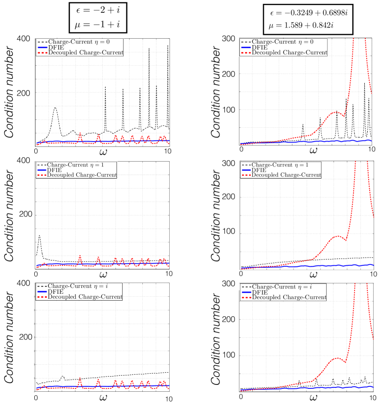
Figure 1: Condition number of the (scaled) DFIE, the charge-current formulation with $\eta=0,1,i$, and the decoupled charge-current (Müller) formulation for a homogeneous dielectric sphere of unit radius as a function of frequency $\omega$ for $\epsilon=-2+i,\mu=-1+i$ and for $\epsilon=-0.3249+0.6898i,\mu=1.589+0.842i$.

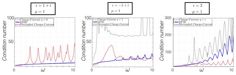
Figure 2: Condition number of the (scaled) DFIE, the charge-current formulation with $\eta=0$, and the decoupled charge-current (Müller) formulation for a homogeneous dielectric sphere of unit radius as a function of frequency $\omega$ for various material parameters.

We plot the locations of spurious resonances of the decoupled charge-current formulation in Fig. 3. For each point in the plane defined by the real parts of $\epsilon$ and $\mu$, we use the scheme described in [14] to find positive imaginary components for $\epsilon$ and $\mu$ that lead to blow-up of the integral equation in the range $\omega\in[0,10]$. The material is lossy (dissipative) by construction, so these resonances are non-physical.

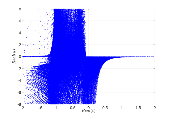
Figure 3: Spurious resonances in the decoupled charge-current formulation.

5 Further numerical validation

While the primary purpose of this paper is to present the derivation and analysis of the decoupled field integral equation, we illustrate its performance here using a high-order locally corrected Nyström discretization [27]. Without entering into details, this method uses $n_{nodes}=7$ points per curved triangular element for 5th order accuracy, $n_{nodes}=25$ points per curved triangular element for 10th order accuracy, and $n_{nodes}=45$ nodes per curved triangular element for 14th order accuracy. The total number of unknowns is $N=6\,N_{tri}\,n_{nodes}$, as there are two tangential vector fields and two scalar unknowns. corresponding to six degrees of freedom, at each point.

For our first example, we consider the obstacle to be a single spheroid centered at the origin with semi-principal axes of length $a=1,b=2$, and $c=3$, with $\epsilon=1.5$ and $\mu=1$, $\epsilon_{0}=\mu_{0}=1$ and $\omega=1$. The incoming wave is assumed to be a plane wave propagating in the $z$-direction. In Fig. 4 we plot the estimated relative error for the interior and exterior regions, using a reference solution with 200 triangles and 45 nodes per triangle.

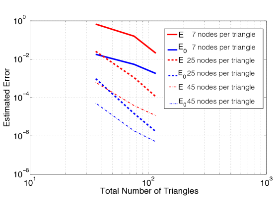
Figure 4: Estimated error for an ellipsoid with semi-principal axes of length $a=1,b=2,c=3$ and $\epsilon=1.5,\mu=1$. The

For our second example, we consider the same ellipsoid with $\omega=1$ but with $\epsilon=-3+i$ and $\mu=-2+.5i$, a so-called double negative index material. Fig. 5 shows the estimated relative error for the interior and exterior regions.

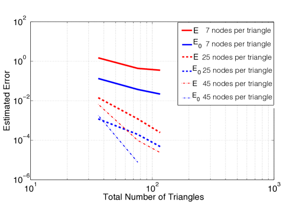
Figure 5: Estimated error for an ellipsoid with semi-principal axes of length $a=1,b=2,c=3$ and $\epsilon=-3+i,\mu=-2+.5i$.

Unlike the naive implementation of Müller’s method (or the PMCHW scheme [20]), there is clearly no “dense-mesh breakdown” in evaluating the electromagnetic field, cconsistent with the theory.

To further demonstrate the stable behavior of our scheme at low frequencies, we consider ithe obstacle to be a sphere of radius $R=1$ with $\epsilon=1.3,\mu=1$. Fig. 6 shows the error, with the exact solution computed via the the Mie solution. There is clearly no low frequency breakdown.

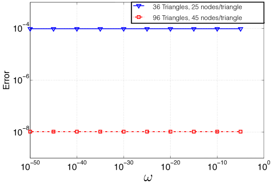
Figure 6: Estimated error for a sphere of radius $R=1$ with $\epsilon=1.3,\mu=1$.

Our final example is a superellipsoid: $x^{8}+y^{8}+z^{8}\leq 1$ with $\epsilon=1.3$, $\mu=1$, and $\omega=0.1$. Fig. 7 shows the estimated relative error for the interior and exterior regions. The error in the exterior region is smaller since it is measured at a distance $R=10$, where the integrals involve smoother integrands. Notice, again, the absence of dense-mesh breakdown.

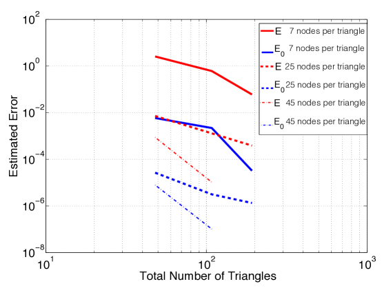
Figure 7: Estimated error for a superellipsoid $x^{8}+y^{8}+z^{8}\leq 1$ with $\epsilon=1.3,\mu=1$.

6 Conclusions

We have presented a new method for simulating electromagnetic scattering from homogeneous penetrable bodies, based on reformulating the Maxwell equations in terms of two uncoupled vector Helmholtz systems. one for the electric feld and one for the magnetic field. We have shown that these partial differential equations have unique solutions and that those solutions correspond to the desired electromagnetic field, Furthermore, we have shown that the vector Helmholtz equations can be recast as boundary integral equations which are well-conditioned and resonance-free for all lossy materials, including doubly negative materials, where $\Re{(\epsilon)}<0,\Re{(\mu)}<0$. We refer to these as decoupled field integral equations. They are insensitive to the genus of the scatterers, and immune from dense-mesh (low frequency) breakdown.

Previously developed charge-current formulations avoid dense-mesh breakdown but can be subject to spurious resonances and can have erratic behavior, as seen in our numerical experiments above. Our approach is based on Fredholm integral equations of the second kind, equipped with relatively straightforward proofs of existence and uniqueness based on standard energy estimates and the Rellich Lemma.

The extension of our method to problems involving both perfect conductors and dielectrics is underway, as is its implementation using suitable fast algorithms. It will be interesting to compare its performance with the generalized Debye method - the only other approach which has been proven to lead to well-posed integral equations for all passive materials [7]. Results from these developments will be reported at a later date.

Appendix A Uniqueness for the Maxwell transmission problem

Theorem 6.

The Maxwell transmission problem has a unique solution for any permittivity and permeability satisfying conditions (6) for $\omega>0$.

Proof.

Suppose that ${\bf E},{\bf H},{\bf E}_{0},{\bf H}_{0}$ denotes a solution to the Maxwell transmission problem with Helmholtz parameters $k^{2}=\omega^{2}\epsilon\mu,k_{0}^{2}=\omega^{2}\epsilon_{0}\mu_{0}$, and homogeneous boundary data, so that

$$\boldsymbol{n}\times\big{(}{\bf E}_{0}-{\bf E}\big{)}=0$$ (50)

$$\boldsymbol{n}\times\Big{(}\frac{\nabla\times{\bf E}_{0}}{\mu_{0}}-\frac{\nabla\times{\bf E}}{\mu}\Big{)}=0.$$

Due to the regularity properties of the fields at the boundary, we may apply the Rellich lemma [3] which states that uniqueness holds if $\Im{E}\geq 0$ where

$$I_{v}=k_{0}\int_{\partial D}\big{(}\boldsymbol{n}\times{\bf E}_{0}\cdot\nabla\times\overline{{\bf E}_{0}}\big{)}ds$$ (51)

and $\Im{E}$ denotes its imaginary part. Using the jump conditions and Green’s identity [3] we obtain:

$$I_{v} =k_{0}\int_{\partial D}\big{(}\boldsymbol{n}\times{\bf E}_{0}\cdot\nabla\times\overline{{\bf E}_{0}}\big{)}ds=k_{0}\overline{\Big{(}\frac{\mu_{0}}{\mu}\Big{)}}\int_{\partial D}\big{(}\boldsymbol{n}\times{\bf E}\cdot\nabla\times\overline{{\bf E}}\big{)}ds=$$ (52)

$$=k_{0}\overline{\Big{(}\frac{\mu_{0}}{\mu}\Big{)}}\int_{D}|\nabla\times{\bf E}|^{2}-\overline{k}^{2}|{\bf E}|^{2}dv=\frac{1}{\overline{\mu}}\Big{(}k_{0}\overline{\mu_{0}}\int_{D}|\nabla\times{\bf E}|^{2}dv\Big{)}+=$$

$$-\overline{\epsilon}\Big{(}k_{0}\omega^{2}\overline{\mu_{0}}\int_{D}|{\bf E}|^{2}dv\Big{)}=\frac{1}{\overline{\mu}}\alpha-\overline{\epsilon}\beta\,.$$

From (6), we find that $\alpha$ and $\beta$ are real, non-negative numbers and $\Im(I_{v})\geq 0$. Thus, ${\bf E}_{0}=0\ \forall\boldsymbol{x}\in\mathbb{R}^{3}/\overline{D}$. Since ${\bf H}_{0}=\frac{\nabla\times{\bf E}_{0}}{i\omega\mu_{0}}$, we also have that ${\bf H}_{0}=0\ \forall\boldsymbol{x}\in\mathbb{R}^{3}/\overline{D}$. From the jump conditions we get $\boldsymbol{n}\times{\bf E}=\boldsymbol{n}\times{\bf H}=0$, therefore, using the representation theorem (see [3]) we get that ${\bf E}=0,{\bf H}=0,\ \forall\boldsymbol{x}\in D$.

We will have occasion to consider the dual case, where $\epsilon,\mu>0$ and $\epsilon_{0},\mu_{0}$ satisfy (6) for which we now show that we the transmission problem also has a unique solution. First, if $\Im(k_{0})=0$, the result above is sufficient. Thus, we may assume that $\Im(k_{0}>0)$. Let $B_{R}$ be a ball with radius $R$ that contains the obstacle $D$. Applying Green’s identity we obtain

$$\frac{1}{\mu_{0}}\int_{\partial B_{R}}\big{(}\boldsymbol{n}\times\overline{{\bf E}_{0}}\cdot\nabla\times{\bf E}_{0}\big{)}ds=\frac{1}{\mu_{0}}\int_{B_{R}/\overline{D}}|\nabla\times{\bf E}_{0}|^{2}-k_{0}^{2}|{\bf E}_{0}|^{2}dv+$$ (53)

$$\qquad\qquad+\frac{1}{\mu}\int_{D}|\nabla\times{\bf E}|^{2}-k^{2}|{\bf E}|^{2}dv.$$

Taking the limit as $R\rightarrow\infty$, the left hand side tends to zero due to the radiation condition and the fact that $\Im(k_{0}>0)$ so that the outer material is lossy. Thus,

$$0=\frac{1}{\mu_{0}}\int_{\mathbb{R}^{3}/\overline{D}}|\nabla\times{\bf E}_{0}|^{2}-k_{0}^{2}|{\bf E}_{0}|^{2}dv+\frac{1}{\mu}\int_{D}|\nabla\times{\bf E}|^{2}-k^{2}|{\bf E}|^{2}dv.$$ (54)

Taking the imaginary part, we get

$$0= \Im\Big{(}\frac{1}{\mu_{0}}\int_{\mathbb{R}^{3}/\overline{D}}|\nabla\times{\bf E}_{0}|^{2}-k_{0}^{2}|{\bf E}_{0}|^{2}dv\Big{)}=$$ (55)

$$= \Im\Big{(}\frac{1}{\mu_{0}}\Big{)}\int_{\mathbb{R}^{3}/\overline{D}}|\nabla\times{\bf E}_{0}|^{2}dv-\Im(\epsilon_{0})\omega^{2}\int_{\mathbb{R}^{3}/\overline{D}}|{\bf E}_{0}|^{2}dv.$$

Recall now that $\mu_{0}$ and $\epsilon_{0}$ cannot both be real. Thus, if $\Im(\mu_{0})>0$, then $\nabla\times{\bf E}_{0}=0$. If $\Im(\epsilon_{0})>0$, then ${\bf E}_{0}=0$. In either case, we get ${\bf H}_{0}={\bf E}_{0}=0\ \forall\boldsymbol{x}\in\mathbb{R}^{3}/\overline{D}$, and ${\bf E}=0,{\bf H}=0,\ \forall\boldsymbol{x}\in D$, as desired. ∎

Remark 3.

At zero frequency, the Maxwell transmission problem no longer has a unique solution, unless additional constraints are imposed on the normal data. Our formulation in terms of the vector electric and magnetic transmission problems is unique even at zero frequency and yields the (unique) limit of the Maxwell transmission problem as $\omega\rightarrow 0^{+}$.

Appendix B The scalar transmission problems

Definition 5.

By the scalar electric transmission problem we mean the calculation of a scalar field

$$u=\left\{\begin{array}[]{ll}u_{i}\in C^{2}(D)\cap C(\overline{D})&\mbox{if $\boldsymbol{x}\in D$};\\ u_{0}\in C^{2}(\mathbb{R}^{3}\setminus\overline{D})\cap C(\mathbb{R}^{3}/D)&\mbox{if $\boldsymbol{x}\in\mathbb{R}^{3}\setminus\overline{D}$},\end{array}\right.$$

with

$$\Delta u_{i}+k^{2}u_{i} =0, \quad\boldsymbol{x} \in D$$ (56)

$$\Delta u_{0}+k_{0}^{2}u_{0} =0, \quad\boldsymbol{x} \in\mathbb{R}^{3}/\overline{D}$$

that satisfies the interface conditions

$$u_{0}-u_{i}=q$$ (57)

$$\frac{1}{\mu_{0}}\frac{\partial u_{0}}{\partial n}-\frac{1}{\mu}\frac{\partial u_{i}}{\partial n}=p$$ (58)

and the Sommerfeld radiation condition

$$\begin{array}[]{ll}\frac{\boldsymbol{x}}{|\boldsymbol{x}|}\cdot\nabla u_{0}(\boldsymbol{x})-ik_{0}u_{0}(\boldsymbol{x})=o\Big{(}\frac{1}{|\boldsymbol{x}|}\Big{)},&|\boldsymbol{x}|\rightarrow\infty\,,\end{array}$$ (59)

where $p,q\in C^{0,\alpha}(\partial D)$. Since we will have occasion to consider the scalar transmission problem satisfied by $u=\nabla\cdot{\bf E}$, and our smoothness assumptions on ${\bf E}$ don’t guarantee differentiability at the boundary, we will sometimes replace the condition (58) wth its weak counterpart:

$$\lim_{h\rightarrow 0,h>0}\int_{\partial D}\left(\frac{1}{\mu_{0}}\frac{\partial u_{0}}{\partial n}(\boldsymbol{x}+h\boldsymbol{n})-\frac{1}{\mu}\frac{\partial u_{i}}{\partial n}(\boldsymbol{x}-h\boldsymbol{n})-p(\boldsymbol{x})\right)w(\boldsymbol{x})ds=0$$ (60)

for all $w(\boldsymbol{x})\in C^{1,\alpha}(\partial D)$.

Definition 6.

By the scalar magnetic transmission problem we mean the calculation of a scalar field

$$v=\left\{\begin{array}[]{ll}v_{i}\in C^{2}(D)\cap C(\overline{D})&\mbox{if $\boldsymbol{x}\in D$};\\ v_{0}\in C^{2}(\mathbb{R}^{3}\setminus\overline{D})\cap C(\mathbb{R}^{3}/D)&\mbox{if $\boldsymbol{x}\in\mathbb{R}^{3}\setminus\overline{D}$},\end{array}\right.$$

with

$$\Delta v_{i}+k^{2}v_{i} =0, \quad\boldsymbol{x} \in D$$ (61)

$$\Delta v_{0}+k_{0}^{2}v_{0} =0, \quad\boldsymbol{x} \in\mathbb{R}^{3}/\overline{D}$$

that satisfies the interface conditions

$$v_{0}-\varphi=q^{\prime}$$ (62)

$$\frac{1}{\epsilon_{0}}\frac{\partial v_{0}}{\partial n}-\frac{1}{\epsilon}\frac{\partial v_{i}}{\partial n}=p^{\prime}$$ (63)

and the Sommerfeld radiation condition (59). Since we will have occasion to consider the scalar transmission problem satisfied by $v=\nabla\cdot{\bf H}$, and our smoothness assumptions on ${\bf H}$ don’t guarantee differentiability at the boundary, we will sometimes replace the condition (63) wth its weak counterpart, as in (60).

Lemma 1.

The scalar electric and magnetic transmission problems have unique solutions for permeabilities and permittivities satisfying (6) for $\omega\geq 0$.

Proof.

We restrict our attention to the electric transmission problem, since the proof for magnetic case is analogous. Thus, Suppose that $\psi,\psi_{0}$ are a solution of the homogeneous scalar electric transmission problem (that is, $p,q=0$). From Theorem 3.3 in [11], we find that the homogeneous solution satisfies the following regularity condition: $\psi_{0}\in C^{2}(\mathbb{R}^{3}/\overline{D})\cap C^{1,\alpha}(\mathbb{R}^{3}/D)$, $\psi\in C^{2}(D)\cap C^{1,\alpha}(\overline{D})$.

First, let us assume that $\omega>0$, $\epsilon_{0},\mu_{0}>0$ and $\epsilon,\mu$ satisfy the material properties given by (6). In order to apply the Rellich lemma we consider the quantity

$$E =k_{0}\int_{\partial D}\psi_{0}\frac{\partial\overline{\psi_{0}}}{\partial n}ds=k_{0}\overline{\Big{(}\frac{\mu_{0}}{\mu}\Big{)}}\int_{\partial D}\psi\frac{\partial\overline{\psi}}{\partial n}ds=k_{0}\overline{\Big{(}\frac{\mu_{0}}{\mu}\Big{)}}\int_{D}|\nabla\psi|^{2}-\overline{k}^{2}|\psi|^{2}dv=$$ (64)

$$=\frac{1}{\overline{\mu}}\Big{(}k_{0}\overline{\mu_{0}}\int_{D}|\nabla\psi|^{2}dv\Big{)}-\overline{\epsilon}\Big{(}\omega^{2}k_{0}\overline{\mu_{0}}\int_{D}|\psi|^{2}dv\Big{)}=\frac{1}{\overline{\mu}}\alpha-\overline{\epsilon}\beta,$$

where $\alpha$ and $\beta$ are real, non-negative numbers. Therefore, $\Im(E)\geq 0$ and $\psi_{0}=0\ \forall\boldsymbol{x}\in\mathbb{R}^{3}/\overline{D}$. From the jump conditions, we get $\psi|_{\partial D}=\frac{\partial\psi}{\partial n}=0$. Therefore, from the representation theorem, we have that $\psi=0\ \forall\boldsymbol{x}\in D$.

Let us now consider the dual problem, where $\epsilon,\mu>0$ and $\epsilon_{0},\mu_{0}$ satisfy (6). If $\Im(k_{0})=0$, then we are in the situation above. Thus, we can assume that $\Im(k_{0}>0)$. Let $B_{R}$ be a ball of radius $R$ that contains the obstacle $D$. Applying Green’s identity we have

$$\frac{1}{\mu_{0}}\int_{\partial B_{R}}\overline{\psi_{0}}\frac{\partial\psi}{\partial n}ds=\frac{1}{\mu_{0}}\int_{B_{R}/\overline{D}}|\nabla\psi_{0}|^{2}-k_{0}^{2}|\psi_{0}|^{2}dv+\frac{1}{\mu}\int_{D}|\nabla\psi|^{2}-k^{2}|\psi|^{2}dv.$$ (65)

Taking the limit $R\rightarrow\infty$, the left-hand side tends to zero due to the radiation condition and the fact that the outer region is lossy. Thus,

$$0=\frac{1}{\mu_{0}}\int_{\mathbb{R}^{3}/\overline{D}}|\nabla\psi_{0}|^{2}-k_{0}^{2}|\psi_{0}|^{2}dv+\frac{1}{\mu}\int_{D}|\nabla\psi|^{2}-k^{2}|\psi|^{2}dv.$$ (66)

Taking the imaginary part, we get

$$0= \Im\Big{(}\frac{1}{\mu_{0}}\int_{\mathbb{R}^{3}/\overline{D}}|\nabla\psi_{0}|^{2}-k_{0}^{2}|\psi_{0}|^{2}dv\Big{)}=\Im\Big{(}\frac{1}{\mu_{0}}\Big{)}\int_{\mathbb{R}^{3}/\overline{D}}|\nabla\psi_{0}|^{2}dv-\Im(\epsilon_{0})\omega^{2}\int_{\mathbb{R}^{3}/\overline{D}}|\psi_{0}|^{2}dv.$$ (67)

Now, $\mu_{0}$ and $\epsilon_{0}$ cannot both be real. If $\Im(\mu_{0})>0$, then $\nabla\psi_{0}=0$. If $\Im(\epsilon_{0})>0$, then $\psi_{0}=0$. In either case, we get $\psi_{0}=0\ \forall\boldsymbol{x}\in\mathbb{R}^{3}/\overline{D}$, and $\psi=0\ \forall\boldsymbol{x}\in D$.

The proof for the static case $\omega=0$ is standard [3]. ∎

Lemma 2.

Let ${\bf E},{\bf E}_{0}$ be a solution of the homogeneous vector electric transmission problem. Then $\psi=\nabla\cdot{\bf E},\psi_{0}=\nabla\cdot{\bf E}_{0}$ satisfy the homogeneous scalar electric transmission problem.

Proof.

Let ${\bf E}_{0},{\bf E}$ be a solution of the homogeneous vector transmission problem. Clearly, the functions $\psi_{0}=\nabla\cdot{\bf E}_{0},\psi=\nabla\cdot{\bf E}$ satisfy the scalar Helmholtz equations $\Delta\psi_{0}+k_{0}^{2}\psi_{0}=0,\Delta\psi+k^{2}\psi=0$ in the corresponding regions, as well as the regularity conditions $\psi_{0}\in C^{2}(\mathbb{R}^{3}/\overline{D})\cap C(\mathbb{R}^{3}/D)$, $\psi\in C^{2}(D)\cap C(\overline{D})$. From (23) we have

$$\psi_{0}-\psi=0.$$ (68)

Let us now assume that $\boldsymbol{n}\times\nabla\times{\bf E}_{0}$ and $\boldsymbol{n}\times\nabla\times{\bf E}$ are sufficiently smooth and that we can take the surface divergence. Then, from (22), (24) and a little algebra, it is easy to check that

$$\frac{1}{\mu_{0}}\frac{\partial\psi_{0}}{\partial n}-\frac{1}{\mu}\frac{\partial\psi}{\partial n}=0.$$ (69)

If $\boldsymbol{n}\times\nabla\times{\bf E}_{0}$ and $\boldsymbol{n}\times\nabla\times{\bf E}$ are merely continuous, let us define the following quantity:

$$I_{1}=\lim_{h\rightarrow 0^{+}}\int_{\partial D}\boldsymbol{n}\cdot\Big{(}\frac{\nabla\times\nabla\times{\bf E}_{0}}{\mu_{0}}(\boldsymbol{x}+h\boldsymbol{n})-\frac{\nabla\times\nabla\times{\bf E}}{\mu_{0}}(\boldsymbol{x}-h\boldsymbol{n})\Big{)}w(\boldsymbol{x})ds\,,$$ (70)

where $\lim_{h\rightarrow 0^{+}}$ implies taking the limit with $h>0$. Using the interface condition (24) it is easy to show that

$$I_{1} =\lim_{h\rightarrow 0^{+}}\int_{\partial D}\boldsymbol{n}\cdot\Big{(}\frac{\nabla\nabla\cdot{\bf E}_{0}}{\mu_{0}}(\boldsymbol{x}+h\boldsymbol{n})-\frac{\nabla\nabla\cdot{\bf E}}{\mu_{0}}(\boldsymbol{x}-h\boldsymbol{n})\Big{)}w(\boldsymbol{x})ds=$$ (71)

$$=\lim_{h\rightarrow 0^{+}}\int_{\partial D}\Big{(}\frac{1}{\mu_{0}}\frac{\partial\psi_{0}}{\partial n}(\boldsymbol{x}+h\boldsymbol{n})-\frac{1}{\mu}\frac{\partial\psi}{\partial n}(\boldsymbol{x}-h\boldsymbol{n})\Big{)}w(\boldsymbol{x})ds.$$

On the other hand, integration by parts yields

$$I_{1} =\lim_{h\rightarrow 0^{+}}\int_{\partial D}\boldsymbol{n}\cdot\Big{(}\frac{\nabla\times\nabla\times{\bf E}_{0}}{\mu_{0}}(\boldsymbol{x}+h\boldsymbol{n})-\frac{\nabla\times\nabla\times{\bf E}}{\mu_{0}}(\boldsymbol{x}-h\boldsymbol{n})\Big{)}w(\boldsymbol{x})ds=$$ (72)

$$=\lim_{h\rightarrow 0^{+}}\int_{\partial D}-\nabla_{s}\cdot\Big{(}\frac{\boldsymbol{n}\times\nabla\times{\bf E}_{0}}{\mu_{0}}(\boldsymbol{x}+h\boldsymbol{n})-\frac{\boldsymbol{n}\times\nabla\times{\bf E}}{\mu_{0}}(\boldsymbol{x}-h\boldsymbol{n})\Big{)}w(\boldsymbol{x})ds=$$

$$=\lim_{h\rightarrow 0^{+}}\int_{\partial D}\Big{(}\frac{\boldsymbol{n}\times\nabla\times{\bf E}_{0}}{\mu_{0}}(\boldsymbol{x}+h\boldsymbol{n})-\frac{\boldsymbol{n}\times\nabla\times{\bf E}}{\mu_{0}}(\boldsymbol{x}-h\boldsymbol{n})\Big{)}\cdot\nabla w(\boldsymbol{x})ds=0,$$

where $\nabla_{s}\cdot\boldsymbol{J}$ is the surface divergence of the tangential vector field $\boldsymbol{J}$, and we have used (22) in the last step. Note that the reason we require this weak formulation is that, in general, we cannot interchange the limit $h\rightarrow 0$ with the surface divergence. ∎

Lemma 3.

Let ${\bf H},{\bf H}_{0}$ be a solution of the homogeneous vector magnetic transmission problem. Then $\varphi=\nabla\cdot{\bf H},\varphi_{0}=\nabla\cdot{\bf H}_{0}$ satisfy the homogeneous scalar magnetic transmission problem.

Proof.

The proof is analogous to that of Lemma 2. ∎

We are now in a position to prove the desired uniqueness result, namely Theorem 1.

Appendix C Proof of Theorem 1

Theorem: The vector electric and magnetic transmission problems have unique solutions for $\omega\geq 0$.

Proof.

Let us assume that $\omega>0$ and that ${\bf E}_{0},{\bf E}$ are a solution of the homogeneous vector electric transmission problem. Then the functions $\psi_{0}=\nabla\cdot{\bf E}_{0},\psi=\nabla\cdot{\bf E}$ satisfy the homogeneous scalar electric transmission problem, and $\psi_{0}=\psi=0$ from Lemma 1.

Thus, ${\bf E}_{0}$ and ${\bf E}$, together with ${\bf H}_{0}:=\frac{\nabla\times{\bf E}_{0}}{i\omega\mu_{0}},{\bf H}:=\frac{\nabla\times{\bf E}}{i\omega\mu}$, constitute an electromagnetic field that satisfies the usual homogeneous interface conditions (continuity fn the tangential electric and magnetic fields). From the uniqueness theorem 6, we may conclude that ${\bf E}_{0}=0,\forall\boldsymbol{x}\in\mathbb{R}^{3}/\overline{D}$ and ${\bf E}=0,\forall\boldsymbol{x}\in D$.

For the static case, $\omega=0$, the theorem is a consequence of the fact that the operators $D_{0},S^{\prime}_{0}$ and $M_{0}$ have a spectrum contained in the interval $[-\frac{1}{2},\frac{1}{2}]$ ([3], Chapter 5). Due to the regularity properties of the solution at the boundary, in particular the fact that $\nabla\cdot{\bf E}_{0},\nabla\times{\bf E}_{0}\in C(\mathbb{R}^{3}/D)$ and $\nabla\cdot{\bf E},\nabla\times{\bf E}\in C(\overline{D})$, we can apply the following representation formula for Laplace vector fields ([3], Theorems 4.11, 4.13):

$$\nabla\times S_{0}[\boldsymbol{n}\times{\bf E}]-S_{0}[\boldsymbol{n}(\nabla\cdot{\bf E})]+S_{0}[\boldsymbol{n}\times\nabla\times{\bf E}]-\nabla S_{0}[\boldsymbol{n}\cdot{\bf E}]=-{\bf E} \boldsymbol{x}\in D$$ (73)

$$\nabla\times S_{0}[\boldsymbol{n}\times{\bf E}_{0}]-S_{0}[\boldsymbol{n}(\nabla\cdot{\bf E}_{0})]+S_{0}[\boldsymbol{n}\times\nabla\times{\bf E}_{0}]-\nabla S_{0}[\boldsymbol{n}\cdot{\bf E}_{0}]={\bf E}_{0} \boldsymbol{x}\in\mathbb{R}^{3}/\overline{D}\,.$$

Taking the curl, we obtain

$$\nabla\times\nabla\times S_{0}[\boldsymbol{n}\times{\bf E}]-\nabla\times S_{0}[\boldsymbol{n}(\nabla\cdot{\bf E})]+\nabla\times S_{0}[\boldsymbol{n}\times\nabla\times{\bf E}]=-\nabla\times{\bf E} \boldsymbol{x}\in D$$ (74)

$$\nabla\times\nabla\times S_{0}[\boldsymbol{n}\times{\bf E}_{0}]-\nabla\times S_{0}[\boldsymbol{n}(\nabla\cdot{\bf E}_{0})]+\nabla\times S_{0}[\boldsymbol{n}\times\nabla\times{\bf E}_{0}]=\nabla\times{\bf E}_{0} \boldsymbol{x}\in\mathbb{R}^{3}/\overline{D}\,.$$

Substracting the tangential components of $\nabla\times{\bf E}$ from those of $\nabla\times{\bf E}_{0}$, and using the jump conditions (21), (22) and (23), we obtain

$$-\frac{\mathbf{f}}{2}\Big{(}1+\frac{\mu}{\mu_{0}}\Big{)}+M_{0}\Big{[}\mathbf{f}\Big{(}1-\frac{\mu}{\mu_{0}}\Big{)}\Big{]}=0,$$ (75)

where $\mathbf{f}=\boldsymbol{n}\times\nabla\times{\bf E}_{0}$. Thus,

$$-\frac{\mathbf{f}}{2}\Big{(}\frac{\mu_{0}+\mu}{\mu_{0}-\mu}\Big{)}+M_{0}(\mathbf{f})=0.$$ (76)

If $\mathbf{f}\neq 0$, then $\Big{(}\frac{\mu_{0}+\mu}{\mu_{0}-\mu}\Big{)}$ must be a real number, say $\lambda$, between $-1$ and $1$ and

$$\Big{(}\frac{\mu_{0}+\mu}{\mu_{0}-\mu}\Big{)}=\lambda\Rightarrow\mu=\mu_{0}\Big{(}\frac{\lambda-1}{\lambda+1}\Big{)}.$$ (77)

As $\mu_{0}>0$, we must have $\mu\leq 0$, a contradiction. Thus, $\mathbf{f}=\boldsymbol{n}\times\nabla\times{\bf E}_{0}=0$. By the jump condition (22) and the fact that boundary data is homogeneous, we have $\boldsymbol{n}\times\nabla\times{\bf E}=0$. The representation formulas (73) are now simplified, taking the form

$$\nabla\times S_{0}[\boldsymbol{n}\times{\bf E}]-S_{0}[\boldsymbol{n}(\nabla\cdot{\bf E})]-\nabla S_{0}[\boldsymbol{n}\cdot{\bf E}]=-{\bf E} \boldsymbol{x}\in D$$ (78)

$$\nabla\times S_{0}[\boldsymbol{n}\times{\bf E}_{0}]-S_{0}[\boldsymbol{n}(\nabla\cdot{\bf E}_{0})]-\nabla S_{0}[\boldsymbol{n}\cdot{\bf E}_{0}]={\bf E}_{0} \boldsymbol{x}\in\mathbb{R}^{3}/\overline{D}\,.$$

Taking the divergence, we have

$$D_{0}[\nabla\cdot{\bf E}]=-\nabla\cdot{\bf E} \boldsymbol{x}\in D$$ (79)

$$D_{0}[\nabla\cdot{\bf E}_{0}]=\nabla\cdot{\bf E}_{0} \boldsymbol{x}\in\mathbb{R}^{3}/\overline{D}\,.$$

Substracting the limiting values from the corresponding sides we obtain

$$-\frac{\nabla\cdot{\bf E}_{0}+\nabla\cdot{\bf E}}{2}+D_{0}[\nabla\cdot{\bf E}_{0}-\nabla\cdot{\bf E}]=0 \ \ \ \boldsymbol{x}\in\partial D.$$ (80)

Using the jump condition (23), we have that $\nabla\cdot{\bf E}_{0}=\nabla\cdot{\bf E}=0\ \forall\boldsymbol{x}\in\partial D$. Thus, the representation formulas (73) simplify even further to

$$\nabla\times S_{0}[\boldsymbol{n}\times{\bf E}]-\nabla S_{0}[\boldsymbol{n}\cdot{\bf E}]=-{\bf E} \boldsymbol{x}\in D$$ (81)

$$\nabla\times S_{0}[\boldsymbol{n}\times{\bf E}_{0}]-\nabla S_{0}[\boldsymbol{n}\cdot{\bf E}_{0}]={\bf E}_{0} \boldsymbol{x}\in\mathbb{R}^{3}/\overline{D}\,.$$

Multiplying the first equation by $\epsilon$ and the second by $\epsilon_{0}$, substracting the tangential components and using the jump condition (24), we obtain

$$-\mathbf{g}\Big{(}\frac{\epsilon_{0}+\epsilon}{2}\Big{)}+M_{0}[\mathbf{g}(\epsilon_{0}-\epsilon)]=0,$$ (82)

where $\mathbf{g}=\boldsymbol{n}\times{\bf E}_{0}$. By the same contradiction argument as above, we find that $\mathbf{g}=0$, so that $\boldsymbol{n}\times{\bf E}_{0}=0,\boldsymbol{n}\times{\bf E}=0$. Thus, the representation formula (73) is simplified again:

$$-\nabla S_{0}[\boldsymbol{n}\cdot{\bf E}]=-{\bf E} \boldsymbol{x}\in D$$ (83)

$$-\nabla S_{0}[\boldsymbol{n}\cdot{\bf E}_{0}]={\bf E}_{0} \boldsymbol{x}\in\mathbb{R}^{3}/\overline{D}.$$

Substracting the normal components, we have

$$-\frac{p}{2}\Big{(}1+\frac{\epsilon_{0}}{\epsilon}\Big{)}-S^{\prime}_{0}\Big{[}p\Big{(}1-\frac{\epsilon_{0}}{\epsilon}\Big{)}\Big{]}=0,$$ (84)

where $p=\boldsymbol{n}\cdot{\bf E}_{0}$. Thus,

$$-\frac{p}{2}\Big{(}\frac{\epsilon_{0}+\epsilon}{\epsilon_{0}-\epsilon}\Big{)}+S^{\prime}_{0}[p]=0.$$ (85)

From the spectral properties of $S^{\prime}$, a simple contradiction argument shows that $\boldsymbol{n}\cdot{\bf E}_{0}=\boldsymbol{n}\cdot{\bf E}=0$. Finally, from the representation formula (73), we have ${\bf E}=0\ \forall\boldsymbol{x}\in D$ and ${\bf E}_{0}=0\ \forall\boldsymbol{x}\in\mathbb{R}^{3}/\overline{D}$.

The proof for the magnetic vector transmission problem is essentially the same. ∎

Appendix D Existence of solutions to the vector transmission problems

Theorem 7.

The vector electric transmission problem has a solution for any $\omega\geq 0$.

Proof.

Let us consider the representation for the solution ${\bf E}_{0},{\bf E}$ given by (36) and the corresponding integral equation (37), obtained by imposing the interface conditions (21) - (24). We examine this Fredholm equation on the product space $C_{t}^{0,\alpha}(Div,\partial D)\times C^{0,\alpha}(\partial D)\times C_{t}^{0,\alpha}(\partial D)\times C^{0,\alpha}(\partial D)$, using the norm

$$\|(\mathbf{a},\sigma,\mathbf{b},\rho)\|\equiv\max\big{(}\|\mathbf{a}\|_{\alpha,\partial D}+\|\nabla_{s}\cdot\mathbf{a}\|_{\alpha,\partial D},\|\sigma\|_{\alpha,\partial D},\|\mathbf{b}\|_{\alpha,\partial D},\|\rho\|_{\alpha,\partial D}\big{)}\,,$$

following the approach of [4]. It will be convenient to rewrite (37) in the form

$$\mathbf{(B+K)x=y}$$ (86)

where

$$\mathbf{B}\equiv\left(\begin{array}[]{cccc}I_{1}&B_{12}&B_{13}&0\\ 0&I_{2}&B_{23}&0\\ 0&0&I_{3}&0\\ B_{41}&0&0&I_{4}\end{array}\right)\,,\quad\mathbf{K}\equiv\left(\begin{array}[]{cccc}K_{11}&0&0&K_{14}\\ 0&K_{22}&0&K_{24}\\ K_{31}&K_{32}&K_{33}&0\\ 0&K_{42}&K_{43}&K_{44}\end{array}\right),$$ (87)

$$\mathbf{x}\equiv\left(\begin{array}[]{c}\boldsymbol{a}\\ \sigma\\ \boldsymbol{b}\\ \rho\end{array}\right),\ \ \mathbf{y}\equiv\left(\begin{array}[]{c}\mathbf{f}\\ q\\ \mathbf{g}\\ p\end{array}\right)\,.$$ (88)

Here,

$$\begin{array}[]{ll}B_{12}=-\boldsymbol{n}\times\big{(}\mu_{0}S_{k_{0}}-\mu S_{k}\big{)}(\boldsymbol{n}\sigma),&B_{13}=\boldsymbol{n}\times\big{(}\mu_{0}\epsilon_{0}S_{k_{0}}-\mu\epsilon S_{k}\big{)}(\boldsymbol{b})\\ B_{23}=\nabla\cdot\Big{(}\mu_{0}\epsilon_{0}S_{k_{0}}-\mu\epsilon S_{k}\Big{)}(\boldsymbol{b}),&B_{41}=\boldsymbol{n}\cdot\nabla\times\big{(}\epsilon_{0}\mu_{0}S_{k_{0}}-\epsilon\mu S_{k}\big{)}(\boldsymbol{a})\\ K_{11}=\big{(}\mu_{0}M_{k_{0}}-\mu M_{k}\big{)}(\boldsymbol{a}),&K_{14}=\boldsymbol{n}\times\nabla\big{(}S_{k_{0}}-S_{k}\big{)}(\rho)\\ K_{22}=\Big{(}\mu_{0}D_{k_{0}}-\mu D_{k}\Big{)}(\sigma),&K_{24}=-\omega^{2}\Big{(}\mu_{0}\epsilon_{0}S_{k_{0}}-\mu\epsilon S_{k}\Big{)}(\rho)\\ K_{31}=\boldsymbol{n}\times\nabla\times\nabla\times\big{(}S_{k_{0}}-S_{k}\big{)}(\boldsymbol{a}),&K_{32}=-\boldsymbol{n}\times\nabla\times\big{(}S_{k_{0}}-S_{k}\big{)}(\boldsymbol{n}\sigma)\\ K_{33}=\big{(}\epsilon_{0}M_{k_{0}}-\epsilon M_{k}\big{)}(\boldsymbol{b}),&K_{42}=-\boldsymbol{n}\cdot\big{(}\epsilon_{0}\mu_{0}S_{k_{0}}-\epsilon\mu S_{k}\big{)}(\boldsymbol{n}\sigma)\\ K_{43}=\boldsymbol{n}\cdot\big{(}\mu_{0}\epsilon_{0}^{2}S_{k_{0}}-\mu\epsilon^{2}S_{k}\big{)}(\boldsymbol{b}),&K_{44}=\big{(}\epsilon_{0}S^{\prime}_{k_{0}}-\epsilon S^{\prime}_{k}\big{)}(\rho)\end{array}$$ (89)

with

$$I_{1}(\boldsymbol{a})=\frac{\mu_{0}+\mu}{2}\boldsymbol{a},\ I_{2}(\sigma)=\frac{\mu_{0}+\mu}{2}\sigma,\ I_{3}(\boldsymbol{b})=\frac{\epsilon_{0}+\epsilon}{2}\boldsymbol{b},\ I_{4}(\rho)=-\frac{\epsilon_{0}+\epsilon}{2}\rho\,.$$

Note that the operators $I_{1},I_{2},I_{3},I_{4}$ are diagonal and invertible from (6). We will denote their inverses by ${\cal I}_{1},{\cal I}_{2},{\cal I}_{3},{\cal I}_{4}$. Note also that the operator $\mathbf{K}$ is compact and that $\mathbf{B}$ is invertible with

$$\mathbf{B}^{-1}=\left(\begin{array}[]{cccc}{\cal I}_{1}&-{\cal I}_{1}{\cal I}_{2}B_{12}&{\cal I}_{1}{\cal I}_{2}{\cal I}_{3}(B_{12}B_{23}-B_{13}I_{2})&0\\ 0&{\cal I}_{2}&-{\cal I}_{2}{\cal I}_{3}B_{23}&0\\ 0&0&{\cal I}_{3}&0\\ -{\cal I}_{1}{\cal I}_{4}B_{41}&{\cal I}_{1}{\cal I}_{2}{\cal I}_{4}B_{12}B_{14}&{\cal I}_{1}{\cal I}_{2}{\cal I}_{3}{\cal I}_{4}(B_{12}B_{23}B_{41}-B_{13}B_{41}I_{2})&{\cal I}_{4}\end{array}\right).$$ (90)

Thus, the Fredholm alternative can be applied and it remains only to show that, in (86), $\mathbf{y}=0$ implies $\mathbf{x}=0$.

For this, we begin by observing that the corresponding fields given by (36) satisfy the homogeneous vector electric transmission problem. By Theorem (1), they must be ${\bf E}_{0}={\bf E}=0$. We now define the following auxiliary fields:

$$\widetilde{{\bf E}_{0}} =-\frac{1}{\mu_{0}}\Big{(}\mu_{0}\nabla\times S_{k_{0}}(\boldsymbol{a})-\mu_{0}S_{k_{0}}(\boldsymbol{n}\sigma)+\mu_{0}\epsilon_{0}S_{k_{0}}(\boldsymbol{b})+\nabla S_{k_{0}}(\rho)\Big{)} \boldsymbol{x}\in D$$ (91)

$$\widetilde{{\bf E}} =\frac{1}{\mu}\Big{(}\mu\nabla\times S_{k}(\boldsymbol{a})-\mu S_{k}(\boldsymbol{n}\sigma)+\mu\epsilon S_{k}(\boldsymbol{b})+\nabla S_{k}(\rho)\Big{)} \boldsymbol{x}\in\mathbb{R}^{3}/\overline{D}.$$

Note that $\widetilde{{\bf E}_{0}}$ is defined in the interior, using the exterior material parameters, and that $\widetilde{{\bf E}}$ is defined in the exterior, using the interior material parameters. From the jump conditions for layer potentials (32), (33), (34), (35), we have

$$\boldsymbol{n}\times\big{(}\frac{{\bf E}_{0}}{\mu_{0}}+\widetilde{{\bf E}_{0}}\big{)} =\boldsymbol{a}$$ (92)

$$\boldsymbol{n}\times\big{(}\frac{\nabla\times{\bf E}_{0}}{\mu_{0}}+\nabla\times\widetilde{{\bf E}_{0}}\big{)} =\epsilon_{0}\boldsymbol{b}$$

$$\boldsymbol{n}\cdot\big{(}\frac{{\bf E}_{0}}{\mu_{0}}+\widetilde{{\bf E}_{0}}\big{)} =-\frac{\rho}{\mu_{0}}$$

$$\frac{\nabla\cdot{\bf E}_{0}}{\mu_{0}}+\nabla\cdot\widetilde{{\bf E}_{0}} =\sigma,$$

and

$$\boldsymbol{n}\times\big{(}\widetilde{{\bf E}}-\frac{{\bf E}}{\mu}\big{)} =\boldsymbol{a}$$ (93)

$$\boldsymbol{n}\times\big{(}\nabla\times\widetilde{{\bf E}}-\frac{\nabla\times{\bf E}}{\mu}\big{)} =\epsilon\boldsymbol{b}$$

$$\boldsymbol{n}\cdot\big{(}\widetilde{{\bf E}}-\frac{{\bf E}}{\mu}\big{)} =-\frac{\rho}{\mu}$$

$$\nabla\cdot\widetilde{{\bf E}}-\frac{\nabla\cdot{\bf E}}{\mu} =\sigma.$$

These, together with the fact that ${\bf E}_{0}={\bf E}=0$, shows that the fields $\widetilde{{\bf E}_{0}},\widetilde{{\bf E}}$ satisfy the jump conditions

$$\boldsymbol{n}\times\Big{(}\widetilde{{\bf E}_{0}}-\widetilde{{\bf E}}\Big{)}=0\\$$ (94)

$$\boldsymbol{n}\times\Big{(}\frac{\nabla\times\widetilde{{\bf E}_{0}}}{\epsilon_{0}}-\frac{\nabla\times\widetilde{{\bf E}}}{\epsilon}\Big{)}=0$$ (95)

$$\boldsymbol{n}\cdot\big{(}\mu_{0}\widetilde{{\bf E}_{0}}-\mu\widetilde{{\bf E}}\big{)}=0$$ (96)

$$\nabla\cdot\widetilde{{\bf E}_{0}}-\nabla\cdot\widetilde{{\bf E}}=0.$$ (97)

By Theorem 1, for the vector magnetic transmission problem (with material properties swapped), we have that $\widetilde{{\bf E}_{0}}=\widetilde{{\bf E}}=0$. Finally, from the jump conditions above, we may conclude that $\boldsymbol{a}=\boldsymbol{b}=0$, $\sigma=\rho=0$. ∎

Theorem 8.

The vector magnetic transmission problem has a solution for any $\omega\geq 0$.

Proof.

The proof is analogous to that of Theorem 7. ∎

Appendix E Proof of Theorem 5

Proof.

It is easy to see that the operators $\mathbf{B}$ and $\mathbf{K}$ in 87 are bounded and compact in the function space $C_{t}^{0,\alpha}(\partial D)\times C^{0,\alpha}(\partial D)\times C_{t}^{0,\alpha}(\partial D)\times C^{0,\alpha}(\partial D)$ with the norm $\|(\mathbf{a},\sigma,\mathbf{b},\rho)\|:=\max\big{(}\|\mathbf{a}\|_{\alpha,\partial D},\|\sigma\|_{\alpha,\partial D},\|\mathbf{b}\|_{\alpha,\partial D},\|\rho\|_{\alpha,\partial D}\big{)}$. As $C_{t}^{0,\alpha}(Div,\partial D)$ is dense in $C_{t}^{0,\alpha}(\partial D)$, the operator $\mathbf{B+K}$ has the same nullspace as in the space analyzed in the proof of Theorem 7 in Appendix D. Thus, it is uniquely solvable. Its inverse operator exists and is bounded as a map from $C_{t}^{0,\alpha}(\partial D)\times C^{0,\alpha}(\partial D)\times C_{t}^{0,\alpha}(\partial D)\times C^{0,\alpha}(\partial D)$ to $C_{t}^{0,\alpha}(\partial D)\times C^{0,\alpha}(\partial D)\times C_{t}^{0,\alpha}(\partial D)\times C^{0,\alpha}(\partial D)$. Due to the collective compactness of the operators, the continuity of the inverse is uniform in $[0,\omega_{\max}]$. This, together with the regularity properties of the operators in (36) [3] implies the desired estimates (41), (42), (43), (44). ∎

References

• [1] W. C. Chew. Vector potential electromagnetics with generalized gauge for inhomogeneous media: formulation. Progress In Electromagnetics Research, 149:69–84, 2014.
• [2] A. Colliander and P. Ylä-Oijala. Electromagnetic scattering from rough surface using single integral equation and adaptive integral method. IEEE Trans. Antennas Propag., 55:3639–3646, 2007.
• [3] D. L. Colton and R. Kress. Integral equation methods in scattering theory. Wiley, New York, 1983.
• [4] D. L. Colton and R. Kress. Inverse acoustic and electromagnetic scattering theory. Springer, New York, 2013.
• [5] K. Cools, F.P. Andriulli, and E. Michielssen. A Calderon multiplicative preconditioner for the PMCHWT integral equation. Antennas and Propagation, IEEE Transactions on, 59(12):4579–4587, Dec 2011.
• [6] M. Costabel and F. Le Louër. On the Kleinman-Martin integral equation method for electromagnetic scattering by a dielectric body. SIAM Journal on Applied Mathematics, 71(2):635–656, 2011.
• [7] C. L. Epstein, L. Greengard, and M. O’Neil. Debye sources and the numerical solution of the time harmonic maxwell equations ii. Communications on Pure and Applied Mathematics, 66(4):753–789, 2013.
• [8] M. Ganesh, S. C. Hawkins, and D Volkov. An all-frequency weakly-singular surface integral equation for electromagnetism in dielectric media: reformulation and well-posedness analysis. Journal of Mathematical Analysis and Applications, 412(1):277–300, 2014.
• [9] Z. Gimbutas and L. Greengard. Fast multi-particle scattering: a hybrid solver for the maxwell equations in microstructured materials. Journal of Computational Physics, 232:22–32, 2013.
• [10] A. Glisson. An integral equation for electromagnetic scattering from homogeneous dielectric bodies. IEEE Trans. Antennas Propag., 32:173–175, 1984.
• [11] Peter Hähner. Eindeutigkeits-und Regularitätssätze für Randwertprobleme bei der skalaren und vektoriellen Helmholtz-Gleichung. Universität zu Göttingen, 1990.
• [12] J. D. Jackson. Classical Electrodynamics. John Wiley & Sons: New York, 1975.
• [13] R. Kress. Minimizing the condition number of boundary integral operators in acoustic and electromagnetic scattering. The Quarterly Journal of Mechanics and Applied Mathematics, 38(2):323–341, 1985.
• [14] R. Kress and G. F. Roach. Transmission problems for the helmholtz equation. Journal of Mathematical Physics, 19(6):1433–1437, 1978.
• [15] E. Marx. Integral equation for scattering by a dielectric. IEEE Trans. Antennas Propag., 32:166–172, 1984.
• [16] J. Mautz. A stable integral equation for electromagnetic scattering from homogenoues dielectric bodies. IEEE Trans. Antennas Propag., 37:1070–1071, 1989.
• [17] C. Müller. Foundations of the mathematical theory of electromagnetic waves. Springer Berlin, 1969.
• [18] Petri Ola P. A. Martin. Boundary integral equations for the scattering of electromagnetic waves by homogeneous dielectric obstacle. Proc. Roy. Soc, 185(208):–, 1993.
• [19] C. H. Papas. Theory of electromagnetic wave propagation. Courier Dover Publications, 1988.
• [20] A. J. Poggio and E. K. Miller. Integral equation solutions of three-dimensional scattering problems. In R. Mittra, editor, Computer Techniques for Electromagnetics, chapter 4, pages 159–264. Pergamon Press, 1973.
• [21] V Rokhlin. Solution of acoustic scattering problems by means of second kind integral equations. Wave Motion, 5(3):257–272, 1983.
• [22] M. Taskinen and S. Vanska. Current and charge integral equation formulations and picard’s extended maxwell system. Antennas and Propagation, IEEE Transactions on, 55(12):3495–3503, 2007.
• [23] M. Taskinen and P. Yla-Oijala. Current and charge integral equation formulation. Antennas and Propagation, IEEE Transactions on, 54(1):58–67, 2006.
• [24] F. Valdes, F. Andriulli, H. Bagci, and E. Michielssen. A calderon-preconditioned single source combined field integral equation for analyzing scattering from homogeneous penetrable objects. IEEE Trans. Antennas Propag., 59:2315–2328, 2011.
• [25] F. Vico, M. Ferrando, L. Greengard, and Z. Gimbutas. The decoupled potential integral equation for time-harmonic electromagnetic scattering. Communications on Pure and Applied Mathematics, 69:771–812, 2016.
• [26] F. Vico, M. Ferrando-Bataller, T. B. Jimenez, and D. Sanchez-Escuderos. A decoupled charge-current formulation for the scattering of homogeneous lossless dielectrics. In 2016 10th European Conference on Antennas and Propagation (EuCAP), pages 1–3. IEEE, 2016.
• [27] F. Vico, M. Ferrando-Bataller, A. Valero-Nogueira, and A. Berenguer. A high-order locally corrected nyström scheme for charge-current integral equations. Antennas and Propagation, IEEE Transactions on, 63(4):1678–1685, 2015.
• [28] F. Vico, L. Greengard, and Z. Gimbutas. Boundary integral equation analysis on the sphere. Numerische Mathematik, 128(3):463–487, 2014.
• [29] T. Von Petersdorff and R. Leis. Boundary integral equations for mixed dirichlet, neumann and transmission problems. Mathematical methods in the applied sciences, 11(2):185–213, 1989.
• [30] M. S. Yeung. Single integral equation for electromagnetic scattering by three-dimensional homogeneous dielectric objects. IEEE Trans. Antennas and Propagation, 47:1615–1622, 1999.
• [31] P. Ylä-Oijala and M. Taskinen. Well-conditioned müller formulation for electromagnetic scattering by dielectric objects. IEEE Transactions on Antennas and Propagation, 53:3316–3323, 2005.
• [32] P. Yla-Oijala, M. Taskinen, and S. Jarvenpaa. Advanced surface integral equation methods in computational electromagnetics. In Electromagnetics in Advanced Applications, 2009. ICEAA’09. International Conference on, pages 369–372. IEEE, 2009.