Circumcentering the Douglas–Rachford method

Abstract

We introduce and study a geometric modification of the Douglas–Rachford method called the Circumcentered–Douglas–Rachford method. This method iterates by taking the intersection of bisectors of reflection steps for solving certain classes of feasibility problems. The convergence analysis is established for best approximation problems involving two (affine) subspaces and both our theoretical and numerical results compare favorably to the original Douglas–Rachford method. Under suitable conditions, it is shown that the linear rate of convergence of the Circumcentered–Douglas–Rachford method is at least the cosine of the Friedrichs angle between the (affine) subspaces, which is known to be the sharp rate for the Douglas–Rachford method. We also present a preliminary discussion on the Circumcentered–Douglas–Rachford method applied to the many set case and to examples featuring non-affine convex sets.

Keywords  Douglas–Rachford method; Best approximation problem; Projection and reflection operators; Friedrichs angle; Linear convergence; Subspaces.

Mathematics Subject Classification (2000)  Primary 49M27, 65K05, 65B99; Secondary 90C25.

1 Introduction

Projection and reflection schemes are celebrated tools for finding a point in the intersection of finitely many sets [15], a basic problem in the natural sciences and engineering (see, e.g., [6] and [17]). Probably the Douglas–Rachford method (DRM) is one of the most famous and well-studied of these schemes (see, e.g.,  [5, 4, 27, 30, 8]). Also known as averaged alternating reflections method, it was introduced in [22] and has recently gained much popularity, in part thanks to its good behavior in non-convex settings (see, e.g., [25, 3, 2, 1, 9, 11, 13, 24, 28]).

This paper has a two-fold aim: (i) improving the original DRM by means of a simple geometric modification, and (ii) meeting the demand of more satisfactory schemes for the many set case.

Regarding (i), the proposed scheme is greedy by means of distance to the solution set, that is, our iterate is the best possible point relying on successive reflections onto two subspaces. In particular, we get an improvement towards the solution set with respect to DRM iteration, which arises from the average of two successive reflections. Also, we get a convergence rate at least as good as DRM’s with a comparable computational effort per iteration, however with numerical results fairly favorable. The aim (ii) will be treated in the last section.

To consider the problem, let $\langle\cdot,\cdot\rangle$ denote the scalar product in $\mathbb{R}^{n}$, $\|\cdot\|$ is the induced norm, that is, the euclidean vector or matrix norm, and $P_{S}$ denotes the orthogonal projection onto a nonempty closed and convex set $S\subset\mathbb{R}^{n}$. The reflection onto $S$ is given by means of $P_{S}$, namely, $R_{S}(x)=(2P_{S}-\operatorname{Id})(x)$, where $\operatorname{Id}$ stands for the identity operator. Note that $P_{S}(x)$ is simply the midpoint of the segment $[x,R_{S}(x)]$.

Our results are established for the following fundamental feasibility problem. Given two subspaces $U$, $V$ of $\mathbb{R}^{n}$ and any point $x\in\mathbb{R}^{n}$, we are interested in solving the best approximation problem [18] of finding the closest point to $x$ in $U\cap V$, i.e.,

$$\text{Find }\bar{x}\in U\cap V\text{ such that }\|\bar{x}-x\|=\min_{w\in U\cap V}\|w-x\|.$$ (1)

For subspaces there exists a nice characterization of the best approximation problem above as $\bar{x}=P_{U\cap V}(x)$ if, and only if, $x-\bar{x}\in(U\cap V)^{\perp}$, i.e.,

$$\langle x-\bar{x},w\rangle=0\qquad\forall\,w\in U\cap V.$$

The classical DRM iteration at a point $x\in\mathbb{R}^{n}$ yields a new iterate $T(x)\in\mathbb{R}^{n}$ given by the midpoint between $x$ and $R_{V}R_{U}(x)$. That is, the Douglas–Rachford (DR) operator $T:\mathbb{R}^{n}\rightarrow\mathbb{R}^{n}$ designed to solve (1) reads as follows

$$T=T_{U,V}\coloneqq\frac{\operatorname{Id}+R_{V}R_{U}}{2}.$$

It is known that, under suitable assumptions, DRM generates a sequence $\{T^{k}(x)\}_{k\in\mathbb{N}}$ converging to the solution of the best approximation problem (1) (see [5]).

Let us now introduce our scheme, called the Circumcentered–Douglas–Rachford method (C–DRM): from a point $x\in\mathbb{R}^{n}$ the next iterate is the circumcenter of the triangle of vertexes $x$, $y\coloneqq R_{U}(x)$ and $z\coloneqq R_{V}R_{U}(x)$, denoted by

$$C_{T}(x)\coloneqq\operatorname{circumcenter}\{x,y,z\}.$$ (2)

By circumcenter we mean that $C_{T}(x)$ is equidistant to $x$, $y$ and $z$ and lies on the affine space defined by these vertexes. For all $x\in\mathbb{R}^{n}$, $C_{T}(x)$ exists, is unique and elementary computable. Existence and uniqueness are obvious if the cardinality of the set $\{x,y,z\}$ is either $1$ or $2$. In fact, if it happens that $x=y=z$, we have $C_{T}(x)=x\in U\cap V$ already — the converse is also true, that is, if $C_{T}(x)=x$, then $x=y=z$. This means that the set of fixed points $\operatorname{Fix}C_{T}$ of the (nonlinear) operator $C_{T}$ is equal to $U\cap V$. If the cardinality $\{x,y,z\}$ is $2$ then $C_{T}(x)$ is the midpoint between the two distinct points. If $x$, $y$ and $z$ are distinct both existence and uniqueness follow from elementary geometry. Thus, one would only have to worry about having a situation in which $x$, $y$ and $z$ are simultaneously distinct and collinear. This cannot happen since reflections onto subspaces are norm preserving. More than that, will further see that the distance of $x$, $y$ and $z$ to $U\cap V$ is exactly the same. Thus, the equidistance we are asking for in (2) turns out to be a necessary condition for a solution of (1).

Note that C–DRM has indeed a $2$-dimensional search flavor: we will show that $C_{T}(x)$ is the closest point to $U\cap V$ belonging to $\operatorname{aff}\{x,y,z\}$, the affine space defined by $x$, $y$ and $z$, whose dimension is equal to $2$, if $x$, $y$ and $z$, are distinct. This property, together with the fact that the DR point $T(x)\in\operatorname{aff}\{x,y,z\}$, is the key to proving a better performance of C–DRM over DRM. An immediate consequence of this nice interpretation is that C–DRM will solve problems in $\mathbb{R}^{2}$ in at most two steps. Figure 1 serves as an intuition guide and illustrates our idea.

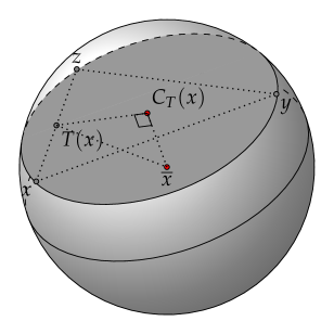
Figure 1: Geometrical interpretation for circumcentering DRM

This paper is organized as follows. In Section 2 we derive the convergence analysis proving that C–DRM has a rate of convergence for solving problem (1) at least as good as DRM’s. Section 3 presents numerical experiments for subspaces along with some non-affine examples in $\mathbb{R}^{2}$. Final remarks as how one can adapt C–DRM for the many set case and other comments on future work are presented in Section 4.

2 Convergence analysis of the Circumcentered–Douglas–Rachford method

In this section we present the theoretical advantages of using C–DRM over the classical DRM iteration for solving (1).

In order to simplify the presentation we recall and fix some notation. For a point $x\in\mathbb{R}^{n}$, we denote for now on $y\coloneqq R_{U}(x)$ and $z\coloneqq R_{V}R_{U}(x)$. Recall that, at the point $x\in\mathbb{R}^{n}$, we define the C–DRM iteration as

$$C_{T}(x)\coloneqq{\rm circumcenter}\{x,y,z\}$$

and the DR iteration (at the same point) is given by

$$T(x)\coloneqq\frac{\operatorname{Id}+R_{V}R_{U}}{2}(x)=\frac{x+z}{2}.$$

In the following we present some elementary facts [18, Theorem 5.8] needed throughout the text.

Proposition 2.1

Let $S$ be a given subspace and $x\in\mathbb{R}^{n}$ arbitrary but fixed. Then, for all $s\in S$ we have:

1. $\langle x-P_{S}(x),s\rangle=0$;

2. $\|x-P_{S}(x)\|^{2}=\|x-s\|^{2}-\|s-P_{S}(x)\|^{2}$;

3. $\|x-s\|=\|R_{S}(x)-s\|$;

4. The projection and reflection mappings $P_{S}$ and $R_{S}$ are linear.

Our first lemma states that the projection of $y$ and $z$ onto $U\cap V$ coincide with $P_{U\cap V}(x)$ and that the distances of $x,y$ and $z$ to $U\cap V$ are the same. In addition to that, we have that the projection of the DR point $T(x)$ onto $U\cap V$ is as well given by $P_{U\cap V}(x)$.

Lemma 2.2

Let $x\in\mathbb{R}^{n}$. Then,

$$P_{U\cap V}(x)=P_{U\cap V}(y)=P_{U\cap V}(z)$$

and

$$\operatorname{dist}(x,U\cap V)=\operatorname{dist}(y,U\cap V)=\operatorname{dist}(z,U\cap V).$$ (3)

Moreover, $P_{U\cap V}(x)=P_{U\cap V}(T(x))$ and

$$P_{U\cap V}(T^{k}(x))\coloneqq P_{U\cap V}(\underbrace{T(\cdots T(T}_{k}(x))\cdots)).$$

Proof. We consider a bar to denote the projection onto the subspace $U\cap V$, i.e., $\bar{x}\coloneqq P_{U\cap V}(x)$, $\bar{y}\coloneqq P_{U\cap V}(y)$, $\bar{z}\coloneqq P_{U\cap V}(z)$, etc. By using Proposition 2.1(iii) for the reflection onto $U$, we get $\|x-w\|=\|y-w\|$ for all $w\in U\cap V$. In particular, $\|x-\bar{y}\|=\|y-\bar{y}\|$ and $\|y-\bar{x}\|=\|x-\bar{x}\|$ since $\bar{x},\bar{y}\in U\cap V$. Therefore,

$$\|x-\bar{x}\|\leq\|x-\bar{y}\|=\|y-\bar{y}\|\leq\|y-\bar{x}\|=\|x-\bar{x}\|,$$

which implies

$$\|x-\bar{x}\|=\|x-\bar{y}\|=\|y-\bar{x}\|=\|y-\bar{y}\|,$$

and, of course, $\operatorname{dist}(x,U\cap V)=\operatorname{dist}(y,U\cap V)$ and $P_{U\cap V}(x)=P_{U\cap V}(y)$ follow.

Now, the statements $\operatorname{dist}(y,U\cap V)=\operatorname{dist}(z,U\cap V)$ and $P_{U\cap V}(y)=P_{U\cap V}(z)$ can be derived by repeating the same argument with $y$ and $z$, where Proposition 2.1(iii) is then considered for the reflection onto $V$. As the projection onto subspaces is linear (Proposition 2.1(iv)) and $T(x)\coloneqq\frac{x+z}{2}$, we have

$$P_{U\cap V}(T(x))=P_{U\cap V}\left(\frac{x+z}{2}\right)=\frac{P_{U\cap V}(x)}{2}+\frac{P_{U\cap V}(z)}{2}=\frac{\bar{x}}{2}+\frac{\bar{x}}{2}=\bar{x}.$$

The rest of the proof follows inductively.

Indeed, we proved $P_{U\cap V}(s)=P_{U\cap V}(T(s))$ for all $s\in\mathbb{R}^{n}$. Then, by setting $s\coloneqq T^{k-1}(x)$, we get

$$P_{U\cap V}(T^{k-1}(x))=P_{U\cap V}(T(T^{k-1}(x)))=P_{U\cap V}(T^{k}(x)),$$

proving the lemma. $\hfill\quad\blacksquare$

We proceed by characterizing $C_{T}(x)$ as the projection of any point $w\in U\cap V$ onto the affine subspace defined by $x,y$ and $z$ denoted by $\operatorname{aff}\{x,y,z\}$.

Lemma 2.3

Let $x\in\mathbb{R}^{n}$ and $W^{x}\coloneqq\operatorname{aff}\{x,y,z\}$. Then,

$$P_{W^{x}}(w)=C_{T}(x),$$

for all $w\in U\cap V$. In particular, $P_{W^{x}}(P_{U\cap V}(x))=C_{T}(x)$.

Proof. Let $w\in U\cap V$ be given and set $p\coloneqq P_{W^{x}}(w)$. Recall that $C_{T}(x)$ is defined by being the only point in $W^{x}$ equidistant to $x$, $y$ and $z$. So, to prove the lemma, we just need to show that $p$ is equidistant to $x$, $y$ and $z$. By Proposition 2.1(ii) we have

$$\|x-p\|^{2} =\|x-w\|^{2}-\|w-p\|^{2},$$

$$\|y-p\|^{2} =\|y-w\|^{2}-\|w-p\|^{2},$$

$$\|z-p\|^{2} =\|z-w\|^{2}-\|w-p\|^{2}.$$

Proposition 2.1(iii) and Lemma 2.2 provided $\|x-w\|=\|y-w\|=\|z-w\|$. Hence, the above equalities imply $\|x-p\|=\|y-p\|=\|z-p\|$, which proves the result. $\hfill\quad\blacksquare$

We have just seen that $C_{T}(x)$ is the closest point in $W^{x}=\operatorname{aff}\{x,y,z\}$ to $U\cap V$. In particular, the circumcenter $C_{T}(x)$ lies at least as close to $U\cap V$ as the DR point $T(x)$.

The next result shows that compositions of $C_{T}(\cdot)$ do not change the projection onto $U\cap V$, that is, for any $x\in\mathbb{R}^{n}$ and $k\in\mathbb{N}$ we have

$$P_{U\cap V}(C^{k}_{T}(x)):=P_{U\cap V}(\underbrace{C_{T}(\cdots C_{T}(C_{T}}_{k}(x))\cdots))=P_{U\cap V}(x).$$

This is a usual feature of algorithms designed to solve best approximation problems.

Lemma 2.4

Let $x\in\mathbb{R}^{n}$ and $k\in\mathbb{N}$. Then,

$$P_{U\cap V}(C_{T}^{k}(x))=P_{U\cap V}(C_{T}(x))=P_{U\cap V}(x).$$

Proof. Note that by proving the second equality, the first follows easily by induction on $k$, likewise the one in the proof of Lemma 2.2. Therefore, let us prove that $P_{U\cap V}(C_{T}(x))=P_{U\cap V}(x)$. Consider again the abbreviation $\bar{x}\coloneqq P_{U\cap V}(x)$ and $\bar{x}_{c}\coloneqq P_{U\cap V}(C_{T}(x))$. From Lemma 2.3 we have that $P_{W^{x}}(\bar{x})=C_{T}(x)$ and also $P_{W^{x}}(\bar{x}_{c})=C_{T}(x)$. Thus, by Pythagoras it follows that

$$\|x-\bar{x}\|^{2} =\|x-C_{T}(x)\|^{2}+\|\bar{x}-C_{T}(x)\|^{2},$$ (4)

$$\|x-\bar{x}_{c}\|^{2} =\|x-C_{T}(x)\|^{2}+\|\bar{x}_{c}-C_{T}(x)\|^{2}.$$ (5)

Now, using again Pythagoras, for the triangles with vertexes $x$, $\bar{x}$, $\bar{x}_{c}$ and $C_{T}(x)$, $\bar{x}_{c}$, $\bar{x}$, we get

$$\|x-\bar{x}_{c}\|^{2} =\|\bar{x}-\bar{x}_{c}\|^{2}+\|x-\bar{x}\|^{2}$$ (6)

and

$$\|C_{T}(x)-\bar{x}\|^{2} =\|\bar{x}-\bar{x}_{c}\|^{2}+\|C_{T}(x)-\bar{x}_{c}\|^{2}.$$ (7)

Then, we obtain

$$\|\bar{x}-\bar{x}_{c}\|^{2}=\|x-\bar{x}_{c}\|^{2}-\|x-\bar{x}\|^{2}=\|\bar{x}_{c}-C_{T}(x)\|^{2}-\|\bar{x}-C_{T}(x)\|^{2}=-\|\bar{x}-\bar{x}_{c}\|^{2},$$

where the first equality follows from (6), the second from subtracting (4) and (5) and the third follows from (7). Thus, $\|\bar{x}-\bar{x}_{c}\|=0$, or equivalently, $\bar{x}=\bar{x}_{c}$. $\hfill\quad\blacksquare$

Note that Lemma 2.4 is related to Fejér monotonicity (see [7, Proposition 5.9 (i)]).

We will now measure the improvement of $C_{T}(x)$ towards $U\cap V$ by means of $x$ and $T(x)$.

Lemma 2.5

For each $x\in\mathbb{R}^{n}$ we have

$$\operatorname{dist}(C_{T}(x),U\cap V)^{2}=\operatorname{dist}(T(x),U\cap V)^{2}-\|T(x)-C_{T}(x)\|^{2}.$$ (8)

In particular,

$$\operatorname{dist}(C_{T}(x),U\cap V)=\|C_{T}(x)-P_{U\cap V}(x)\|\leq\|T(x)-P_{U\cap V}(x)\|=\operatorname{dist}(T(x),U\cap V).$$

Proof. Lemma 2.3 says in particular that $P_{W^{x}}(P_{U\cap V}(x))=C_{T}(x)$, which is equivalent to saying that $\left\langle{s-C_{T}(x)},{P_{U\cap V}(x)-C_{T}(x)}\right\rangle=0$ for all $s$ on the affine subspace $W^{x}$. Now, taking $T(x)$ for the role of $s$ and using Pythagoras, we get (8), since $P_{U\cap V}(C_{T}(x))=P_{U\cap V}(T(x))=P_{U\cap V}(x)$ due to Lemmas 2.2 and 2.4. The rest of the result is direct consequence of Lemmas 2.4 and 2.2. $\hfill\quad\blacksquare$

The linear rate of convergence we are going to derive for C–DRM is given by the cosine of the Friedrichs angle between $U$ and $V$, defined below.

Definition 2.6

The cosine of the Friedrichs angle $\theta_{F}$ between $U$ and $V$ is given by

$$c_{F}(U,V)\coloneqq\sup\big{\{}{\left\langle{u},{v}\right\rangle}\leavevmode\nobreak\ \big{|}\leavevmode\nobreak\ {u\in U\cap(U\cap V)^{\perp},\;v\in V\cap(U\cap V)^{\perp},\;\|u\|\leq 1,\;\|v\|\leq 1}\big{\}}.$$

If context permits, we use just $c_{F}$ instead of $c_{F}(U,V)$.

Next we state some fundamental properties of the Friedrichs angle.

Proposition 2.7

Let $U,V\subset\mathbb{R}^{n}$ be subspaces, then:

1. $0\leq c_{F}(U,V)=c_{F}(V,U)=c_{F}(U^{\perp},V^{\perp})<1$.

2. $c_{F}=\|P_{V}P_{U}-P_{U\cap V}\|=\|P_{V^{\perp}}P_{U^{\perp}}-P_{U^{\perp}\cap V^{\perp}}\|$.

Proof. (i) See [20, Theorems 13 and 16]; (ii): See [18, Lemma 9.5(7)]. $\hfill\quad\blacksquare$

The following result is an elementary fact in Linear Algebra and will be used in sequel.

Proposition 2.8

Let a subspace $S\subset\mathbb{R}^{n}$ be given. If $x,p\in\mathbb{R}^{n}$ are such that their midpoint

$$s\coloneqq\frac{x+p}{2}\in S,$$

then $\operatorname{dist}(x,S)=\operatorname{dist}(p,S)$.

Proof. Let $s\coloneqq\frac{x+p}{2}\in S$, $\hat{x}\coloneqq P_{S}(x)$ and $\hat{p}\coloneqq P_{S}(p)$. Set $\tilde{p}\coloneqq\hat{x}+2(s-\hat{x})\in S$ and note that $\tilde{p}$ is defined in such a way that the triangle with vertexes $x$, $\hat{x}$ and $s$ is congruent to the triangle formed by $p$, $\tilde{p}$ and $s$. In particular, $\|\tilde{p}-p\|=\|x-\hat{x}\|$. Therefore,

$$\|\hat{p}-p\|\leq\|\tilde{p}-p\|=\|x-\hat{x}\|.$$ (9)

An analogous construction can be considered for the triangle with vertexes $p$, $\hat{p}$ and $s$ and the one with vertexes $x$, $\tilde{x}$ and $s$, where $\tilde{x}\coloneqq\hat{p}+2(s-\hat{p})\in S$, yielding $\|\hat{x}-x\|\leq\|\tilde{x}-x\|=\|p-\hat{p}\|$. This, combined with (9), proves the proposition. $\hfill\quad\blacksquare$

The next lemma organizes and summarizes known properties of sequences generated by DRM, some of which will be important in the proof of our main theorem. It is worth noting that items (i) and (vi) are novel to our knowledge.

Lemma 2.9

Let $x\in\mathbb{R}^{n}$ be given. Then, the following assertions for DRM hold:

1. $\operatorname{dist}(T^{k}(x),U+V)=\operatorname{dist}(x,U+V)$ for all $k\in\mathbb{N}$, where $U+V=\operatorname{span}(U\cup V)$;

2. The set $\operatorname{Fix}T\coloneqq\big{\{}{x\in\mathbb{R}^{n}}\leavevmode\nobreak\ \big{|}\leavevmode\nobreak\ {T(x)=x}\big{\}}$ is given by $\operatorname{Fix}T=(U\cap V)\oplus(U^{\perp}\cap V^{\perp})$;

3. The DRM sequence $\{T^{k}(x)\}_{k\in\mathbb{N}}$ converges to $P_{\operatorname{Fix}T}(x)$ and for all $k\in\mathbb{N}$,

   $$\|T^{k}(x)-P_{\operatorname{Fix}T}(x)\|\leq c^{k}_{F}\|x-P_{\operatorname{Fix}T}(x)\|;$$

4. For all $k\in\mathbb{N}$ we have $P_{U\cap V}(T^{k}(x))=P_{U\cap V}(x)$ and $P_{\operatorname{Fix}T}(T^{k}(x))=P_{\operatorname{Fix}T}(x)$;

5. $P_{U\cap V}(x)=P_{\operatorname{Fix}T}(x)$ if, and only if, $x\in U+V$;

6. The DRM sequence $\{T^{k}(x)\}_{k\in\mathbb{N}}$ converges to $P_{U\cap V}(x)$ if, and only if,

   $$x\in U+V;$$

7. The shadow sequences

   $$\{P_{U}(T^{k}(x))\}_{k\in\mathbb{N}}\text{ and }\{P_{V}(T^{k}(x))\}_{k\in\mathbb{N}}$$

   converge to $P_{U\cap V}(x)$.

Proof. For the sake of notation set $S\coloneqq U+V$ and remind that $y\coloneqq R_{U}(x)$ and $z\coloneqq R_{V}(y)$. We have $\frac{1}{2}(x+y)=P_{U}(x)\in S$ and $\frac{1}{2}(y+z)=P_{V}(y)\in S$. Employing Proposition 2.8 yields $\operatorname{dist}(x,S)=\operatorname{dist}(y,S)=\operatorname{dist}(z,S)$. Also, $\frac{1}{2}(T(x)+y)=\frac{1}{2}(\frac{x+z}{2}+y)=\frac{1}{2}(P_{U}(x)+P_{V}(y))\in S$. Using again Proposition 2.8 we conclude that $\operatorname{dist}(T(x),S)=\operatorname{dist}(y,S)$. Hence, $\operatorname{dist}(T(x),S)=\operatorname{dist}(x,S)$ for all $x\in\mathbb{R}^{n}$. A simple induction procedure gives us $\operatorname{dist}(T^{k}(x),U+V)=\operatorname{dist}(x,U+V)$ for all $k\in\mathbb{N}$, proving (i).

The proofs of items (ii), (iii), (iv) and (vii) are in [5].

It is straightforward to check that $S^{\perp}=U^{\perp}\cap V^{\perp}$. Therefore, $\operatorname{Fix}T$ specialized to $S$ reduces to $U\cap V$ and (v) follows. (vi) is a combination of (ii) and (v). $\hfill\quad\blacksquare$

We are now in the position to present our main convergence result, which states that the best approximation problem (1) can be solved for any point $x\in\mathbb{R}^{n}$ with usage of C–DRM.

Theorem 2.10

Let $x\in\mathbb{R}^{n}$ be given. Then, the three C–DRM sequences

$$\{C_{T}^{k}(P_{U}(x))\}_{k\in\mathbb{N}},\{C_{T}^{k}(P_{V}(x))\}_{k\in\mathbb{N}}\text{ and }\{C_{T}^{k}(P_{U+V}(x))\}_{k\in\mathbb{N}}$$

converge linearly to $P_{U\cap V}(x)$. Moreover, their rate of convergence is at least the cosine of the Friedrichs angle $c_{F}\in[0,1)$.

Proof. Obviously, $u,v,s\in U+V$, with $u\coloneqq P_{U}(x)$, $v\coloneqq P_{V}(x)$ and $s\coloneqq P_{U+V}(x)$. Let us first prove that $\bar{u}=\bar{v}=\bar{x}\coloneqq P_{U\cap V}(x)$, where $\bar{u}\coloneqq P_{U\cap V}(u)$, $\bar{v}\coloneqq P_{U\cap V}(v)$ and $\bar{s}\coloneqq P_{U\cap V}(s)$. The definition of $\bar{u},\bar{x}$ allow us to employ Pythagoras and conclude that

$$\|u-x\|^{2}+\|u-\bar{x}\|^{2}=\|x-\bar{x}\|^{2}\leq\|x-\bar{u}\|^{2}=\|u-x\|^{2}+\|u-\bar{u}\|^{2},$$

which provides $\|u-\bar{x}\|=\|u-\bar{u}\|$. Thus $\bar{u}=\bar{x}$. We get $\bar{v}=\bar{s}=\bar{x}$ analogously, and by item (v) of Lemma 2.9 we further have $\bar{u}=P_{\operatorname{Fix}T}(u)=\bar{v}=P_{\operatorname{Fix}T}(v)=\bar{s}=P_{\operatorname{Fix}T}(s)=\bar{x}$. Hence, it holds that

$$\|C_{T}(u)-\bar{x}\|=\|C_{T}(u)-\bar{u}\| \leq\|T(u)-\bar{u}\|=\|T(u)-P_{\operatorname{Fix}T}(u)\|$$

$$\leq c_{F}\|u-P_{\operatorname{Fix}T}(u)\|=c_{F}\|u-\bar{x}\|,$$

where the first inequality is by Lemma 2.5 and the second one by item (iii) of Lemma 2.9. Recall that Lemma 2.4 stated that $P_{U\cap V}(C_{T}^{k}(P_{U}(x)))=P_{U\cap V}(P_{U}(x))$ for all $k\in\mathbb{N}$. So, $P_{U\cap V}(C_{T}^{k}(u))=P_{U\cap V}(u)=\bar{x}$ for all $k\in\mathbb{N}$. Consider now the induction hypothesis $\|C_{T}^{k-1}(u)-\bar{x}\|\leq c_{F}^{k-1}\|u-\bar{x}\|$ for some $k-1$ — the case $k-1=1$ was seen above — and note that

$$\|C_{T}^{k}(u)-\bar{x}\| =\|C_{T}(C_{T}^{k-1}(u))-P_{U\cap V}(C_{T}^{k-1}(u))\|$$

$$\leq\|T(C_{T}^{k-1}(u))-P_{U\cap V}(C_{T}^{k-1}(u))\|$$

$$\leq c_{F}\|C_{T}^{k-1}(u)-P_{U\cap V}(C_{T}^{k-1}(u))\|$$

$$=c_{F}\|C_{T}^{k-1}(u)-\bar{x}\|\leq c_{F}c_{F}^{k-1}\|u-\bar{x}\|=c_{F}^{k}\|u-\bar{x}\|,$$

where the first inequality is due to Lemma 2.5. The second inequality above follows from Lemma 2.9 (iii) and (v), since $u\in U+V$, and the third is by the induction hypothesis. This proves the theorem for the sequence $\{C_{T}^{k}(P_{U}(x))\}$. The proof lines for the convergence of the sequences $\{C_{T}^{k}(P_{V}(x))\}$ and $\{C_{T}^{k}(P_{U+V}(x))\}$ with the linear rate $c_{F}$ are analogous. $\hfill\quad\blacksquare$

An immediate consequence is stated below.

Corollary 2.11

Let $x\in U+V$ be given. Then, the C–DRM sequence $\{C_{T}^{k}(x)\}_{k\in\mathbb{N}}$ converges linearly to $P_{U\cap V}(x)$. Moreover, the rate of convergence is at least the cosine of the Friedrichs angle $c_{F}\in[0,1)$.

Although we believe that Theorem 2.10 holds for $\{C_{T}^{k}(x)\}$ itself, it is worth mentioning that considering the initial feasibility step $P_{U}(x)$ or $P_{V}(x)$ is totally reasonable, since we are assuming that the projection/reflection operators $P_{U}$, $P_{V}$, $R_{U}$ and $R_{V}$ are available. In addition to that, these feasibility steps keep the whole C–DRM sequence in $U+V$, which can be very desirable. In this sense, let us look at two distinct lines $U,V\subset\mathbb{R}^{3}$ intersecting at the origin and assume that their Friedrichs angle is not ninety degrees, i.e., $c_{F}\in(0,1)$. C–DRM finds the origin after one or two steps when starting in $U+V$, since $U+V$ is the plane containing the two lines. If the initial point is not in $U+V$ and no feasibility step is taken, C–DRM may generate an infinite sequence. Therefore, running C–DRM in $U+V$, a potentially smaller set than $\mathbb{R}^{n}$, sounds attractive from the numerical point of view.

The feasibility procedure employed in Theorem 2.10 provides convergence to best approximation solutions for the DRM without the need of considering shadow sequences. This is formally presented in the following.

Corollary 2.12

Let $x\in\mathbb{R}^{n}$ be given. Then, the three DRM sequences

$$\{T^{k}(P_{U}(x))\}_{k\in\mathbb{N}},\;\{T^{k}(P_{V}(x))\}_{k\in\mathbb{N}}\;\text{ and }\;\{T^{k}(P_{U+V}(x))\}_{k\in\mathbb{N}}$$

converge linearly to $P_{U\cap V}(x)$. Moreover, their rate of convergence is given by the cosine of the Friedrichs angle $c_{F}\in[0,1)$.

Proof. This result follows from the fact that $P_{U\cap V}(P_{U}(x))=P_{U\cap V}(P_{V}(x))=P_{U\cap V}(P_{U+V}(x))=P_{U\cap V}(x)$, established within the proof of Theorem 2.10, combined with Lemma 2.9 (vi). $\hfill\quad\blacksquare$

It is known that $c_{F}$ is the sharp rate for DRM [5]. This is not clear for C–DRM though and left as an open question in this work. One way of addressing this issue would be looking at the magnitude of improvement of C–DRM over DRM given by (8) in Lemma 2.5.

We finish this section by showing that Theorem 2.10 and Corollaries 2.11 and 2.12 are applicable to affine subspaces with nonempty intersection, where the concept of the cosine of the Friedrichs angle is suitably extended.

Corollary 2.13

Let $A$ and $B$ be affine subspaces of $\mathbb{R}^{n}$ with nonempty intersection and $p\in A\cap B$ arbitrary but fixed. Then, Theorem 2.10 and Corollaries 2.11 and 2.12 hold for $A$ and $B$, with the rate $c_{F}$ being the cosine of the Friedrichs angle between the subspaces $U_{A}\coloneqq A-\{p\}$ and $V_{B}\coloneqq B-\{p\}$.

Proof. Since $p\in A\cap B$, the translations $A-\{p\}$ and $B-\{p\}$ provide nonempty subspaces $U_{A}$ and $V_{B}$. Now, the elementary translation properties of reflections $R_{U_{A}}(x)+p=R_{A}(x+p)$ and $R_{V_{B}}(x)+p=R_{B}(x+p)$ give us the translation formulas for the correspondent Douglas-Rachford and circumcentering operators:

$$T_{A,B}(x+p)\coloneqq T_{U_{A},V_{B}}(x)+p$$

and

$$C_{T_{A,B}}(x+p)\coloneqq C_{T_{U_{A},V_{B}}}(x)+p,$$

for all $x\in\mathbb{R}^{n}$. This suffices to prove the corollary when setting $U\coloneqq U_{A}$ and $V\coloneqq V_{B}$ in Theorem 2.10 and Corollaries 2.11 and 2.12, because the above formulas imply that $T_{A,B}^{k}(x+p)=T_{U_{A},V_{B}}^{k}(x)+p$ and $C_{T_{A,B}}^{k}(x+p)=C_{T_{U_{A},V_{B}}}^{k}(x)+p$, for all $k\in\mathbb{N}$.

$\hfill\quad\blacksquare$

Simple manipulations let us conclude that $c_{F}=c_{F}(U_{A},V_{B})$, with $U_{A}$ and $V_{B}$ as above, does not depend on the particular choice of the point $p$ in $A\cap B$. Therefore, $c_{F}$ can be referred to as the cosine of the Friedrichs angle between the affine subspaces $A$ and $B$ with no ambiguity.

We finish this section remarking that the computation of circumcenters is possible in arbitrary inner product spaces — see (10). However, projecting/reflecting onto subspaces depends on their closedness. Now, in Hilbert spaces, it is well known that having $c_{F}$ strictly smaller than $1$ is equivalent to asking $U+V$ to be closed [20, Theorem 13]. This is an assumption that maintains the linear convergence in Hilbert spaces for several projection/reflection methods and that would also enable us to extend our main results concerning C–DRM to an infinite dimensional setting.

The following section is on numerical experiments and begins by showing how one can compute $C_{T}(x)$ by means of elementary and cheap Linear Algebra operations.

3 Numerical experiments

In this section, we make use of numerical experiments to show, as a proof of concept, that the good theoretical proprieties of $C_{T}(x)$ are also working in practical problems.

First, for a given point $x\in\mathbb{R}^{n}$, we establish a procedure to find $C_{T}(x)$. We then discuss the stopping criteria used in our experiments and show the performance of C–DRM compared to DRM applied to problem (1). We also apply C–DRM and DRM to non-affine samples, which are not treated theoretically in the previous section. The experiments with these problems indicate as well a good behavior of C–DRM over DRM. All experiments were performed using julia [12] programming language and the pictures were generated using PGFPlots [23].

3.1 How to compute the circumcenter in $\mathbb{R}^{n}$

In order to compute $C_{T}(x)$, recall that $y\coloneqq R_{U}(x)$ and $z\coloneqq R_{V}(y)=R_{V}R_{U}(x)$. We have already mentioned that $C_{T}(x)=x$ if, and only if, the cardinality of $\operatorname{aff}\{x,y,z\}$ is 1. If this cardinality is 2, $C_{T}(x)$ is the midpoint between the two distinct points.

Therefore, we will focus on the computation of $C_{T}(x)$ for the case where $x$, $y$ and $z$ are distinct. According to Lemma 2.3, $C_{T}(x)$ is still well defined, and it can be seen as the circumcenter of the triangle $\Delta xyz$ formed by the points $x$, $y$ and $z$, as illustrated in Figure 2. Also, $T(x)$ lies in $\operatorname{aff}\{x,y,z\}$.

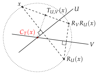
Figure 2: Circumcenter on the affine subspace $\operatorname{aff}\{x,y,z\}$.

Let $x$ be the anchor point of our framework and define $s_{U}\coloneqq y-x$ and $s_{V}\coloneqq z-x$, the vectors pointing from $x$ to $y$ and from $x$ to $z$, respectively. Note that $\operatorname{aff}\{x,y,z\}=x+\operatorname{span}\{s_{U},s_{V}\}$, and since $C_{T}(x)\in\operatorname{aff}\{x,y,z\}$, the dimension of the ambient space, namely $n$, is irrelevant to the geometry. The problem is intrinsically a $2$-dimensional one, regardless of what $n$ is.

We want to find the vector $s\in\operatorname{aff}\{x,y,z\}$, whose projection onto each vector $s_{U}$ and $s_{V}$ has its endpoint at the midpoint of the line segment from $x$ to $y$ and $x$ to $z$, that is,

$$P_{\operatorname{span}\{s_{U}\}}(s)=\frac{1}{2}s_{U}\quad\text{ and }\quad P_{\operatorname{span}\{s_{V}\}}(s)=\frac{1}{2}s_{V}.$$

This requirement yields

$$\begin{cases}\left\langle s_{U},s\right\rangle=\frac{1}{2}\|s_{U}\|^{2},\\ \left\langle s_{V},s\right\rangle=\frac{1}{2}\|s_{V}\|^{2}.\end{cases}$$

By writing $s=\alpha s_{U}+\beta s_{V}$ we get the $2\times 2$ linear system with unique solution $(\alpha,\beta)$

$$\begin{cases}\alpha\|s_{U}\|^{2}+\beta\left\langle s_{U},s_{V}\right\rangle=\frac{1}{2}\|s_{U}\|^{2},\\ \alpha\left\langle s_{U},s_{V}\right\rangle+\beta\|s_{V}\|^{2}=\frac{1}{2}\|s_{V}\|^{2}.\end{cases}$$ (10)

Hence,

$$C_{T}(x)=x+\alpha s_{U}+\beta s_{V}.$$

Note that (10) enables us to calculate $C_{T}(x)$ in arbitrary inner product spaces.

3.2 The case of two subspaces

In our experiments we randomly generate $100$ instances with subspaces $U$ and $V$ in $\mathbb{R}^{200}$ such that $U\cap V\neq\{0\}$. Each instance is run for $20$ initial random points. Based on Theorem 2.10 and Corollary 2.12, we monitor the C–DRM sequence $\{C_{T}^{k}(P_{V}(x))\}$ and the DRM sequence $\{T^{k}(P_{V}(x))\}$. Note that the DRM sequence will always converge to $U\cap V$, since $P_{V}(x)\in U+V$. For the C–DRM sequence, such hypothesis does not seem to be necessary, however for the sake of fairness, we choose to monitor this sequence in the same way. We incorporate the method of alternating projections (MAP) (see, e.g., [19]) in our experiments as well. MAP generates a sequence $\{(P_{V}P_{U})^{k}(x)\}$ that lies automatically in $U+V$ for all $k\geq 1$.

Let $\{s^{k}\}$ be any of the three sequences that we monitor. We considered two tolerances

$$\varepsilon_{1}\coloneqq 10^{-3}\text{ and }\varepsilon_{2}\coloneqq 10^{-6},$$

and employed two stopping criteria:

• the true error, given by $\|s^{k}-\bar{x}\|<\varepsilon_{i};$ and

• the gap distance, given by $\|P_{U}(s^{k})-P_{V}(s^{k})\|<\varepsilon_{i},$ for $i=1,2$.

We performed tests with two tolerances in order to challenge C–DRM by asking for more precision. Also, one can view the true error as the best way to assure one is sufficiently close to $U\cap V$, and in our case $\bar{x}\coloneqq P_{U\cap V}(x)$ is easily available. However, this is not the case in applications, thus, we also utilized the gap distance, which we consider a reasonable measure of infeasibility.

In order to represent the results of our numerical experiments, we used the Performance Profiles [21], a analytic tool that allows one to compare several different algorithms on a set of problems with respect to a performance measure or cost, which in our case is the number of iterations, providing the visualization and interpretation of the results of benchmark experiments. The rationale of choosing number of iterations as performance measure here is that in each of the sequences that are monitored, the majority of the computational cost involved is equivalent — two orthogonal projections onto the subspaces $U$ and $V$ per iteration have to be computed for each method. The graphics were generated using perprof-py [29].

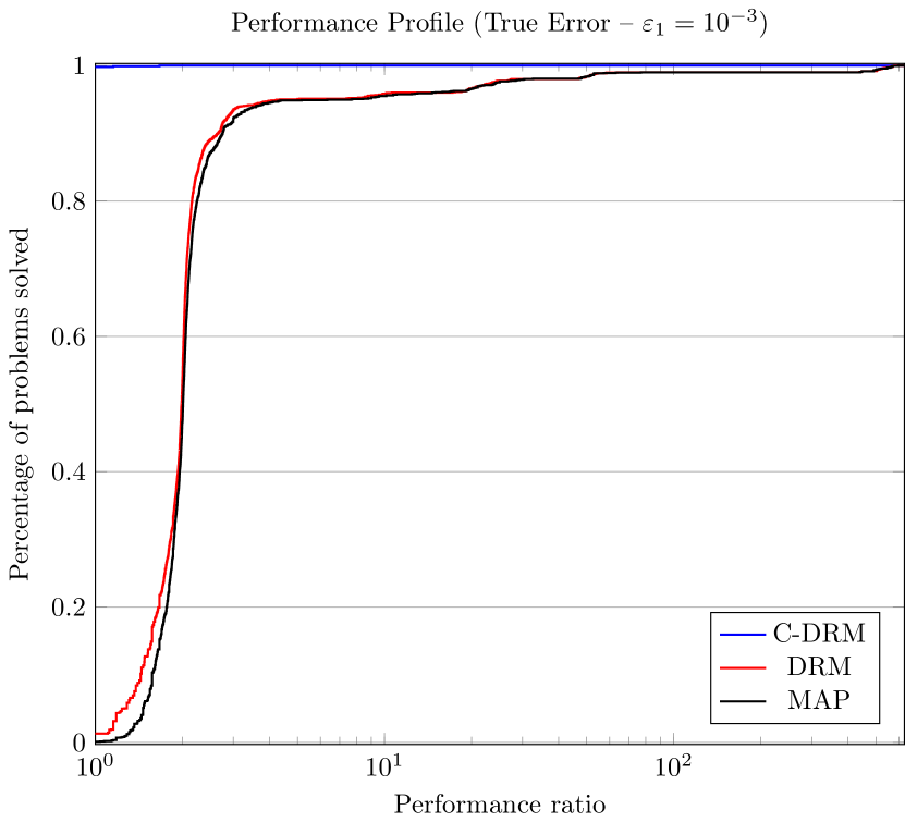
(a)

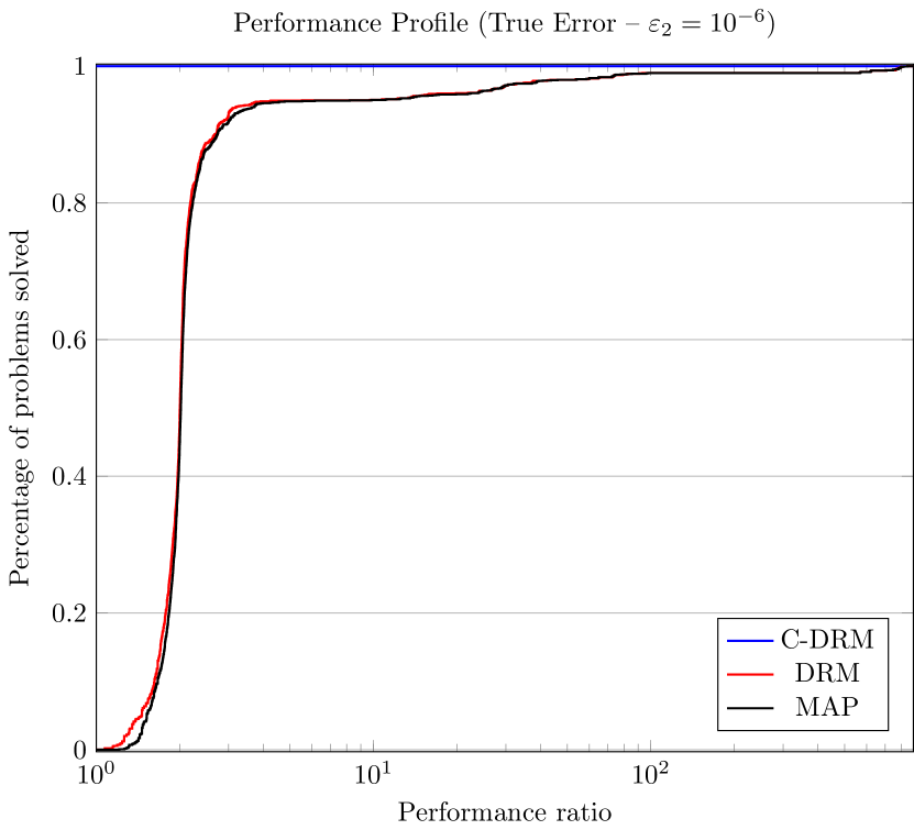
(b)

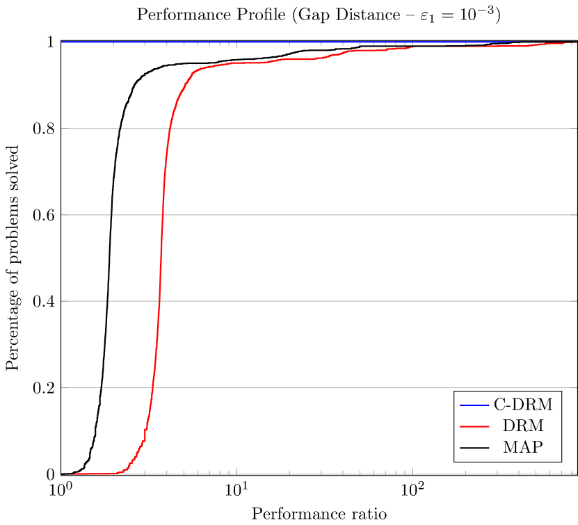
(c)

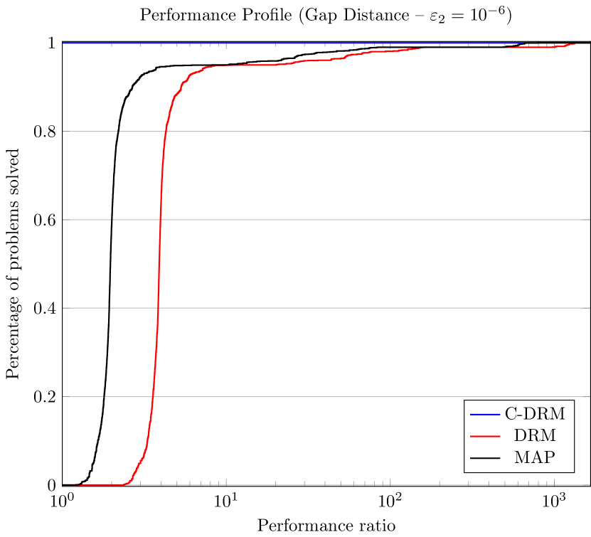
(d)

Figure 3: Experiments with two subspaces.

The numerical experiments shown in Figure 3 confirm the theoretical results obtained in this paper, since C–DRM has a much better performance than DRM. For $\varepsilon_{2}=10^{-6}$, C–DRM solves all instances and choices of initial points in less iterations than DRM, regardless the stopping criteria (See Figures 3(b) and 3(d)). For $\varepsilon_{1}=10^{-3}$, using the true error criteria, according to Figure 3(a) a tiny part of the instances were solved faster by DRM, however this behavior was not reproduced with the gap distance criteria (see Figure 3(d)). MAP has $c_{F}^{2}$ as asymptotic linear rate (see [26]) and it was beaten by C–DRM in all our instances. This gives rise to the interesting question of whether the rate $c_{F}^{2}$ can be theoretically achieved by C–DRM.

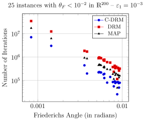
(a)

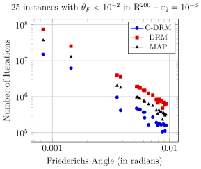
(b)

Figure 4: Experiments with two subspaces having a small Friederichs angle.

Figure 4 represents experiments in which the Friederichs angle between the two subspaces is smaller than $10^{-2}$ and the true error criterion is used. In this case, MAP and DRM are known to converge slowly. C–DRM, however, handled the small values of the Friederichs angle substantially better.

3.3 Some non-affine examples

Next we present two simple classes of examples revealing the potential of the proposed modification when it is applied to the convex and the non-convex case. Here we are using the gap distance with $\varepsilon_{2}=10^{-6}$.

Example 3.1 (Two balls in $\mathbb{R}^{2}$)

We present three figures that depict numerical experiments showing the behavior of C–DRM over DRM concerning the problem of finding a point in the intersection of two convex balls in $\mathbb{R}^{2}$.

Note that Lemma 2.5 shows that $C_{T}(x)$ is closer to $U\cap V$ than $T(x)$ for problem (1). Unfortunately, this is not true in general for convex sets. Figure 5(a), illustrates this for two balls. Here, $x^{0}$ is the starting point, $\bar{x}=P_{U\cap V}(x^{0})$ is the only point in the intersection, $x_{C}^{1}\coloneqq C_{T}(x^{0})$ and $x_{DR}^{1}\coloneqq T(x^{0})$. Note however, that this does not mean that C–DRM will not work for the general case. Even though $x_{DR}^{1}$ is closer to $\bar{x}$ than $x_{C}^{1}$ is, C–DRM performed way less iterations (37) than DRM (971) to find the solution.

Below we present two examples, in Figures 5(b) and 5(c), where the two balls intersection is still compact but has infinitely many points. Depending on the starting point, we achieve different results, regarding the number of iterations that both C–DRM and DRM take to converge. Moreover, Figure 5(b) shows that the accumulation point of the sequences generated by C–DRM and DRM are not necessarily the same, with comparable iteration complexity though. In Figure 5(c), DRM converged after 6 iterations while C–DRM took 7 iterations.

(a)

(b)

(c)

Figure 5: Experiments with two balls in $\mathbb{R}^{2}$.

We performed extensive experiments featuring two convex balls in $\mathbb{R}^{n}$ with starting points being chosen randomly, and the results were very similar to the ones presented in the pictures above. These positive experiments show that it might be possible to use C–DRM to find a point in the intersection of non-affine convex sets. This should be sought in the future. Note however, that C–DRM need not be defined in the general convex setting. This may be the case when an iterate happens to reach the line passing through the centers of the balls in our examples. Therefore, a hybrid strategy is necessary in order to have C–DRM generating an infinite sequence.

Example 3.2 (A ball and a line and a circle and a line in $\mathbb{R}^{2}$)

Our examples show that C–DRM is likely to converge in less iterations than DRM. Also, as important as algorithmic complexity, is convergence to a solution itself.

(a)

(b)

(c)

Figure 6: Experiments with a ball and a line in $\mathbb{R}^{2}$.

In this regard, we underline that our pictures clearly display that C–DRM converges faster than DRM to a solution of problem (1). Moreover, DRM fails to find the unique common point of the ball and the line (only converging in the matter of shadow sequences) and to find the best approximation point in Figure 6(a) and Figure 6(b), respectively.

Figure 6(c) represents a slightly non-convex example with a circle and a line, which was considered for DRM in [11]. In this experiment both C–DRM and DRM converge and the latter was slower. This reveals an interesting and promising property of C–DRM, as well as DRM, when it is applied to non-convex problems. To end this discussion, it is worth mentioning that we performed extensive numerical tests for particular instances of non-convex problem in $\mathbb{R}^{n}$ and the results are very positive. This is a humble attempt in targeting the problem of finding a point in the intersection of an affine subspace with the $s$–space vectors defined by the generalized $\ell_{0}$–ball (see problem (6) of [25]).

4 Conclusions and future work

We have introduced and derived a convergence analysis for the Circumcentered–Douglas–Rachford method (C–DRM) for best approximation problems featuring two (affine) subspaces $U,V\subset\mathbb{R}^{n}$. For any initial point, linear convergence to the best solution was shown and the rate of convergence of C–DRM was proven to be at least as good as DRM’s. DRM is known to converge with the sharp rate $c_{F}\in[0,1)$, the cosine of the Friedrichs angle between $U$ and $V$ (see, e.g., [5]). A question, left as open in this paper, is whether $c_{F}$ is a sharp rate for C–DRM. In this regard, our numerical experiments show that circumcentering “speeds up” convergence of DRM for two subspaces as well as for most of our simple non-affine examples.

In view of future work, we end the paper with a brief discussion on the many set case and on how one can “circumcenter” other classical projection/reflection type methods.

The many set case. Another relevant advantage of the circumcentering scheme C–DRM is that it can be extended to the following many set case.

Assume that $\{U_{i}\}_{i=1}^{m}\subset\mathbb{R}^{n}$ is a family of finitely many affine subspaces with nonempty intersection $\cap_{i=1}^{m}U_{i}$ and that we are interested in projecting onto $\cap_{i=1}^{m}U_{i}$ using knowledge provided by reflections onto each $U_{i}$.

For an arbitrary initial point $x\in\mathbb{R}^{n}$ we could consider a generalized C–DRM iteration by taking the circumcenter $C_{T}(x)$ of

$$\{x,R_{U_{1}}(x),R_{U_{2}}R_{U_{1}}(x),\ldots,R_{U_{m}}\cdots R_{U_{2}}R_{U_{1}}(x)\},$$

i.e., $C_{T}(x)$ is in $\operatorname{aff}\{x,R_{U_{1}}(x),R_{U_{2}}R_{U_{1}}(x),\ldots,R_{U_{m}}\cdots R_{U_{2}}R_{U_{1}}(x)\}$ and

$$\operatorname{dist}(C_{T}(x),x)=\operatorname{dist}(C_{T}(x),R_{U_{1}}(x))=\cdots=\operatorname{dist}(C_{T}(x),R_{U_{m}}\cdots R_{U_{2}}R_{U_{1}}(x)).$$

The fact that $C_{T}(x)$ is well defined and that it is precisely given by the projection of any point in $\cap_{i=1}^{m}U_{i}$ onto

$$W^{x}\coloneqq\operatorname{aff}\{x,R_{U_{1}}(x),R_{U_{2}}R_{U_{1}}(x),\ldots,R_{U_{m}}\cdots R_{U_{2}}R_{U_{1}}(x)\}$$

can be derived similarly as in Lemma 2.3. We understand though, that the convergence analysis of C–DRM for the many set case might be substantially more challenging, since we no longer can rely on the theory of DRM. Also, one should note that now, for large $m$, the computation of $C_{T}(x)$ may not be negligible. This computation consists of finding the intersection of $m$ bisectors in $W^{x}$. Therefore, linear system (10) is now $m\times m$, and the calculation of $C_{T}(x)$ requires its resolution.

If, for a given problem, the computation of $C_{T}(x)$ mentioned above is simply too demanding, one could, e.g., consider pairwise circumcenters or even other ways of circumcentering. The important thing here is that we can enforce several strategies to help overcome the unsatisfactory extension of the classical Douglas–Rachford method for the many set case. It is known that for an example in $\mathbb{R}^{2}$ with three distinct lines intersecting at the original (see [2, Example 2.1]), the natural extension of the Douglas–Rachford method may fail to find a solution. On the other hand, any reasonable circumcentering scheme will solve this particular problem in at most two steps for any initial point. Circumcentering schemes may also be embedded in methods for the many set case, e.g., CADRA [10] and the Cyclic–Douglas–Rachford method [14].

Circumcentering other reflection/projection type methods. For the case of $U$ and $V$ being affine subspaces, the reflected Cimmino method [16] considers a current point $x\in\mathbb{R}^{n}$ and takes the next iterate as the mean $\frac{1}{2}(R_{U}(x)+R_{V}(x))$. Circumcentering the Cimmino method is possible by setting the next iterate as $\operatorname{circumcenter}\{x,R_{U}(x),R_{V}(x)\}$. Something similar can be done for the Method of Alternating Projections (MAP) (see e.g. [19]). From a point $x\in\mathbb{R}^{n}$, MAP moves to $P_{V}P_{U}(x)$. In order to circumcenter MAP, one could take the circumcenter of $x$, $R_{U}(x)$ and $R_{V}P_{U}(x)$. The coherence of this approach lies on the fact that the mid points of the segments $[x,R_{U}(x)]$ and $[P_{U}(x)$, $R_{V}P_{U}(x)]$ are $P_{U}(x)\in U$ and $P_{V}P_{U}(x)\in V$, respectively. Note that both the Circumcentered–Cimmino–Method and the Circumcentered–MAP solve problems with affine subspaces $U,V\subset\mathbb{R}^{2}$ in at most two steps. This happens because circumcentering can be seen as a $2$-dimensional hyperplane search for the two set case.

Finally, we consider that investigating C–DRM for general convex feasibility problems [6] may be fruitful.

Acknowledgements

We thank the anonymous referees for their valuable suggestions.

References

- [1] Francisco J Aragón Artacho, Jonathan M Borwein and Matthew K Tam “Global behavior of the Douglas–Rachford method for a nonconvex feasibility problem” In Journal of Global Optimization 65.2, 2016, pp. 309–327
- [2] Francisco J Aragón Artacho, Jonathan M Borwein and Matthew K Tam “Recent Results on Douglas–Rachford Methods for Combinatorial Optimization Problems” In Journal of Optimization Theory and Applications 163.1, 2014, pp. 1–30
- [3] Francisco J Aragón Artacho and Jonathan M Borwein “Global convergence of a non-convex Douglas–Rachford iteration” In Journal of Global Optimization 57.3, 2013, pp. 753–769
- [4] Heinz H Bauschke, Jose Yunier Bello Cruz, Tran T A Nghia, Hung M Phan and Xianfu Wang “Optimal Rates of Linear Convergence of Relaxed Alternating Projections and Generalized Douglas-Rachford Methods for Two Subspaces” In Numerical Algorithms 73.1, 2016, pp. 33–76
- [5] Heinz H Bauschke, Jose Yunier Bello Cruz, Tran T A Nghia, Hung M Phan and Xianfu Wang “The rate of linear convergence of the Douglas–Rachford algorithm for subspaces is the cosine of the Friedrichs angle” In Journal of Approximation Theory 185, 2014, pp. 63–79
- [6] Heinz H Bauschke and Jonathan M Borwein “On Projection Algorithms for Solving Convex Feasibility Problems” In Siam Review 38.3, 2006, pp. 367–426
- [7] Heinz H Bauschke and Patrick L Combettes “Convex Analysis and Monotone Operator Theory in Hilbert Spaces”, CMS Books in Mathematics Cham: Springer International Publishing, 2017
- [8] Heinz H Bauschke and Walaa M Moursi “On the Douglas–Rachford algorithm” In Mathematical Programming 164.1-2, 2016, pp. 263–284
- [9] Heinz H Bauschke and Dominikus Noll “On the local convergence of the Douglas–Rachford algorithm” In Archiv der Mathematik 102.6, 2014, pp. 589–600
- [10] Heinz H Bauschke, Dominikus Noll and Hung M Phan “Linear and strong convergence of algorithms involving averaged nonexpansive operators” In Journal of Mathematical Analysis and Applications 421.1, 2015, pp. 1–20
- [11] Joël Benoist “The Douglas–Rachford algorithm for the case of the sphere and the line” In Journal of Global Optimization 63.2, 2015, pp. 363–380
- [12] Jeff Bezanson, Alan Edelman, Stefan Karpinski and Viral B Shah “Julia: A Fresh Approach to Numerical Computing” In Siam Review 59.1, 2017, pp. 65–98
- [13] Jonathan M Borwein and Brailey Sims “The Douglas–Rachford Algorithm in the Absence of Convexity” In Fixed-Point Algorithms for Inverse Problems in Science and Engineering New York, NY: Springer New York, 2011, pp. 93–109
- [14] Jonathan M Borwein and Matthew K Tam “A Cyclic Douglas–Rachford Iteration Scheme” In Journal of Optimization Theory and Applications 160.1, 2014, pp. 1–29
- [15] Yair Censor and Andrzej Cegielski “Projection methods: an annotated bibliography of books and reviews” In Optimization 64.11, 2014, pp. 2343–2358
- [16] Gianfranco Cimmino “Calcolo approssimato per le soluzioni dei sistemi di equazioni lineari” In La Ricerca Scientifica 9.II, 1938, pp. 326–333
- [17] P L Combettes “The foundations of set theoretic estimation” In Proceedings of the IEEE 81.2, 1993, pp. 182–208
- [18] Frank R Deutsch “Best Approximation in Inner Product Spaces”, CMS Books in Mathematics New York, NY: Springer New York, 2001
- [19] Frank R Deutsch “Rate of Convergence of the Method of Alternating Projections” In Parametric Optimization and Approximation: Conference Held at the Mathematisches Forschungsinstitut, Oberwolfach, October 16–22, 1983 Basel: Birkhäuser Basel, 1985, pp. 96–107
- [20] Frank R Deutsch “The Angle Between Subspaces of a Hilbert Space” In Approximation Theory, Wavelets and Applications Dordrecht: Springer Netherlands, 1995, pp. 107–130
- [21] Elisabeth D Dolan and Jorge J Moré “Benchmarking optimization software with performance profiles” In Mathematical Programming 91.2, 2002, pp. 201–213
- [22] Jim Douglas and H H Rachford “On the numerical solution of heat conduction problems in two and three space variables” In Transactions of the American Mathematical Society 82.2, 1956, pp. 421–421
- [23] Christian Feuersänger “PGFPlots Package”, 2016
- [24] Robert Hesse and D Russell Luke “Nonconvex Notions of Regularity and Convergence of Fundamental Algorithms for Feasibility Problems”, 2013, pp. 2397–2419
- [25] Robert Hesse, D Russell Luke and Patrick Neumann “Alternating Projections and Douglas-Rachford for Sparse Affine Feasibility” In IEEE Transactions on Signal Processing 62.18, 2014, pp. 4868–4881
- [26] Selahattin Kayalar and Howard L Weinert “Error bounds for the method of alternating projections” In Mathematics of Control, Signals and Systems 1.1, 1988, pp. 43–59
- [27] P Lions and B Mercier “Splitting Algorithms for the Sum of Two Nonlinear Operators” In SIAM Journal on Numerical Analysis 16.6, 1979, pp. 964–979
- [28] Hung M Phan “Linear convergence of the Douglas–Rachford method for two closed sets” In Optimization 65.2, 2016, pp. 369–385
- [29] Abel Soares Siqueira, Raniere Costa Silva and Luiz-Rafael Santos “Perprof-py: A Python Package for Performance Profile of Mathematical Optimization Software” In Journal of Open Research Software 4.e12, 2016, pp. 5
- [30] Benar F Svaiter “On Weak Convergence of the Douglas–Rachford Method” In SIAM Journal on Control and Optimization 49.1, 2011, pp. 280–287