Inhomogeneous fluid of penetrable-spheres: application of the random phase approximation

Abstract

The focus of the present work is the application of the random phase approximation (RPA), derived for inhomogeneous fluids [Frydel and Ma, Phys. Rev. E 93, 062112 (2016)], to penetrable-spheres. As penetrable-spheres transform into hard-spheres with increasing interactions, they provide an interesting case for exploring the RPA, its shortcomings, and limitations, the weak- versus the strong-coupling limit. Two scenarios taken up by the present study are a one-component and a two-component fluid with symmetric interactions. In the latter case, the mean-field contributions cancel out and any contributions from particle interactions are accounted for by correlations. The accuracy of the RPA for this case is the result of a somewhat lucky cancellation of errors.

I Introduction

Recently in Ref. 1 we have extended the random phase approximation (RPA) to inhomogeneous fluids as a systematic attempt to supplement the mean-field description with correlations Frydel16b . When that approximation is applied to Coulomb particles, one finds the same set of equations as those constituting the variational Gaussian approximation within the field-theoretical framework generated by transforming the original partition function into a functional integral Netz00 ; Wang10 ; Tony14 ; David14 ; Frydel15 . (The variational Gaussian approximation for ions consists of two coupled equations. One is the Poisson-Boltzmann equation with a modified charge density that includes correlational contributions. And the second equation determines correlational contributions and can be represented as the Ornstein-Zernike (OZ) equation, suggesting an alternative derivation within the density functional theory.) It then follows that the variational Gaussian approximation is nothing other than the RPA approximation formulated within a different framework. The density functional formulation, however, not only offers an alternative derivation. Its greatest merit is that it provides generalization to any particle system as the formulation makes no assumptions about pair interactions. The question then is not for what pair interactions, but rather under what conditions the RPA is reliable. The conditions at which the RPA fails for penetrable-spheres should be general and apply to Coulomb particles or the Gaussian core model. Defining the limits of the validity of the RPA for one system, therefore, offers insights about those limits in another system.

Because the RPA approach of Ref. Frydel16 is non-perturbative (correlations and density are obtained self-consistently), it is tempting to think it is suitable for describing the strong-coupling limit. However, the study of Ref. Frydel16 for a number of pair interactions does not support this conjecture. If anything, it suggests the contrary view that the RPA, despite its non-perturbative feature, is strictly a theory of weakly correlated systems. Again, by identifying the variational Gaussian approximation of the field-theoretical formulation as the RPA, this conclusion is not surprising. The RPA has been used for long time in the electronic structure DFT where it?s known as a theory of the weakly-correlated limit Ren12 . One goal of this paper, therefore, is to dispel the misunderstanding that the variational Gaussian approximation has potential for describing the strong-coupling regime of a charged or any system.

In Ref. Frydel16 we applied the RPA to Coulomb particles and the Gaussian core model (considered to be a weakly correlated fluid Hansen00a ; Evans01 ; Frydel16c ). In the present work, we continue to explore the RPA by its application to penetrable-spheres. Unlike hard-spheres, penetrable-spheres may overlap, however, every overlap incurs energy cost. As overlaps become more costly, penetrable-spheres transform into hard-spheres. As the RPA is not expected to work for hard-spheres, one should observe a gradual breakdown of the RPA as a function of increasing interactions. The case of penetrable-spheres, therefore, provides a useful testing ground for the performance of the RPA.

In Sec. II we lay down the framework of the RPA approximation. In Sec. III we investigate a homogenous case of penetrable-spheres. In Sec. IV we show the results for an inhomogeneous fluid near a planar wall. In Sec. V we consider alternative (dilute limit) approaches and compare them with the RPA. In Sec. VI we study a two-component penetrable-sphere fluid with symmetric interactions. Finally, in Sec. VII we conclude the work.

II The random phase approximation

In this section we go over the construction of the RPA approximation. We begin with the expression for the mean-field free energy,

$$F_{\rm mf}[\rho] = F_{\rm id}[\rho]+\int\!d{\bf r}\,\rho({\bf r})U({\bf r})$$ (1)

$$+ \frac{1}{2}\int\!d{\bf r}\!\int\!d{\bf r}^{\prime}\rho({\bf r})\rho({\bf r}^{\prime})u({\bf r},{\bf r}^{\prime}).$$

The last term captures particle interactions, however, it neglects correlations which complete the free energy expression as

$$F[\rho]=F_{\rm mf}[\rho]+F_{c}[\rho].$$ (2)

The exact expression for $F_{c}[\rho]$ is obtained using the adiabatic connection wherein pair interactions $\lambda u({\bf r},{\bf r}^{\prime})$ are gradually switched on as $\lambda$ varies from $0\to 1$. During the procedure the density $\rho({\bf r})$ is kept fixed by means of an external $\lambda$-dependent potential, $U_{\lambda}({\bf r})$, which in the limit $\lambda\to 1$ recovers a true external potential. Keeping a density independent of $\lambda$ is essential for constructing a density functional formulation.

Defining the free energy for a given $\lambda$ as $F_{\lambda}=-k_{B}T\log Z_{\lambda}$ where

$$Z_{\lambda}=\frac{1}{N!\Lambda^{3N}}\!\!\int\!\!d{\bf r}_{1}\!\dots\!\!\int\!\!d{\bf r}_{N}\,e^{-\beta\sum_{i}U_{\lambda}({\bf r}_{i})}e^{-\beta\lambda\sum_{j>i}u({\bf r}_{i},{\bf r}_{j})},$$ (3)

and $N$ is the total number of particles, the free energy of a physical system at $\lambda=1$ is given by

$$F=F_{\lambda=0}+\int_{0}^{1}d\lambda\,\frac{\partial F_{\lambda}}{\partial\lambda}.$$ (4)

After some substitution and manipulation we get the free energy expression where the correlational part is found to be

$$F_{c}[\rho]=\frac{1}{2}\int_{0}^{1}d\lambda\int d{\bf r}\,\rho({\bf r})\int d{\bf r}^{\prime}\,\rho({\bf r}^{\prime})h_{\lambda}({\bf r},{\bf r}^{\prime})u({\bf r},{\bf r}^{\prime}),$$ (5)

where $h_{\lambda}({\bf r},{\bf r}^{\prime})$ is the correlation function of a fluid Hansen with interactions $\lambda u({\bf r},{\bf r}^{\prime})$ and in the presence of the external potential $U_{\lambda}({\bf r})$, which although absent in Eq. (5) is implied by a fixed $\rho({\bf r})$.

To complete the framework we still need a way to calculate $h_{\lambda}({\bf r},{\bf r}^{\prime})$. To this end we introduce the Ornstein-Zernike equation (OZ),

$$h_{\lambda}({\bf r},{\bf r}^{\prime})=c_{\lambda}({\bf r},{\bf r}^{\prime})+\int d{\bf r}^{\prime\prime}\,\rho({\bf r}^{\prime\prime})h_{\lambda}({\bf r}^{\prime},{\bf r}^{\prime\prime})c_{\lambda}({\bf r},{\bf r}^{\prime\prime}),$$ (6)

which expresses $h_{\lambda}({\bf r},{\bf r}^{\prime})$ in terms of the direct correlation function $c_{\lambda}({\bf r},{\bf r}^{\prime})$. A direct correlation function is obtained from the exact definition,

$$c_{\lambda}({\bf r},{\bf r}^{\prime})\equiv-\beta\frac{\delta^{2}F_{ex}^{\lambda}[\rho]}{\delta\rho({\bf r})\delta\rho({\bf r}^{\prime})},$$ (7)

and since we are interested in a systematic method beyond the mean-field, we use the mean-field result for the excess free energy, $F_{\rm ex}\approx\frac{1}{2}\int d{\bf r}\int d{\bf r}^{\prime}\rho({\bf r})\rho({\bf r}^{\prime})u({\bf r},{\bf r}^{\prime})$, which yields

$$c_{\lambda}^{\rm rpa}({\bf r},{\bf r}^{\prime})=-\lambda\beta u({\bf r},{\bf r}^{\prime}).$$ (8)

The above is known as the random phase approximation closure. Inserting this into the OZ equation we get

$$h_{\lambda}^{\rm rpa}({\bf r},{\bf r}^{\prime}) = -\lambda\beta u({\bf r},{\bf r}^{\prime})$$ (9)

$$- \lambda\beta\int d{\bf r^{\prime\prime}}\,\rho({\bf r}^{\prime\prime})h_{\lambda}^{\rm rpa}({\bf r}^{\prime\prime},{\bf r}^{\prime})u({\bf r},{\bf r}^{\prime\prime}),$$

and the correlation free energy becomes

$$F_{c}^{\rm rpa}[\rho]=-\frac{1}{2}\int d{\bf r}\rho({\bf r})\int_{0}^{1}d\lambda\,\frac{h_{\lambda}^{\rm rpa}({\bf r},{\bf r})+\lambda\beta u({\bf r},{\bf r})}{\lambda\beta}.$$ (10)

$h_{\lambda}^{\rm rpa}({\bf r},{\bf r}^{\prime})$ can alternatively be represented as an expansion

$$h_{\lambda}^{\rm rpa}({\bf r},{\bf r}^{\prime})=-\beta\lambda u({\bf r},{\bf r}^{\prime})$$ (11)

$$+ \beta^{2}\lambda^{2}\int\!\!d{\bf r}_{1}\,\rho({\bf r}_{1})u({\bf r},{\bf r}_{1})u({\bf r}_{1},{\bf r}^{\prime})$$

$$- \beta^{3}\lambda^{3}\int\!\!d{\bf r}_{1}\!\!\int\!\!d{\bf r}_{2}\,\rho({\bf r}_{1})\rho({\bf r}_{2})u({\bf r},{\bf r}_{1})u({\bf r}_{1},{\bf r}_{2})u({\bf r}_{2},{\bf r}^{\prime})$$

$$+ \dots$$

generated by repetitive substitution of $h_{\lambda}({\bf r},{\bf r}^{\prime})$ each time it appears on the right-hand side of the OZ equation.

Using the above expansion, the correlation free energy becomes

$$\beta F_{c}^{\rm rpa}[\rho] = -\frac{\beta^{2}}{4}\!\!\int\!\!d1\!\!\int\!\!d2\,\rho_{1}\rho_{2}u_{12}u_{21}$$ (12)

$$+ \frac{\beta^{3}}{6}\!\!\int\!\!d1\!\!\int\!\!d2\!\!\int\!\!d3\,\rho_{1}\rho_{2}\rho_{3}u_{12}u_{23}u_{31}$$

$$- \frac{\beta^{4}}{8}\!\!\int\!\!d1\!\!\int\!\!d2\!\!\int\!\!d3\!\!\int\!\!d4\,\rho_{1}\rho_{2}\rho_{3}\rho_{4}u_{12}u_{23}u_{34}u_{41}$$

$$+ \dots$$

where $\rho({\bf r}_{i})\to\rho_{i}$, $u({\bf r}_{i},{\bf r}_{j})\to u_{ij}$, and $\int d{\bf r}_{i}\to\int di$. All the constituent integral terms have a ring topology, a mathematical signature of the RPA.

The above expansion is handy for generating functional derivatives. For example, a true density satisfies the relation $\frac{\delta F}{\delta\rho}=\mu$, where $\mu$ denotes the chemical potential. A functional derivative of $F_{c}$ with respect to $\rho({\bf r})$ is carried out term by term, leading to a new expansion that is identified as

$$\frac{\delta\beta F_{c}^{\rm rpa}[\rho]}{\delta\rho({\bf r})}=-\frac{1}{2}\bigg{(}h^{\rm rpa}({\bf r},{\bf r})+\beta u({\bf r},{\bf r})\bigg{)}.$$ (13)

A physical density then satisfies

$$\rho({\bf r}) = \rho_{b}e^{-\beta U({\bf r})}e^{-\beta\int d{\bf r}^{\prime}\,[\rho({\bf r}^{\prime})-\rho_{b}]u({\bf r},{\bf r}^{\prime})}$$ (14)

$$\times e^{\frac{1}{2}[h^{\rm rpa}({\bf r},{\bf r})-h^{\rm rpa}_{b}(0)]},$$

where $\rho_{b}$ is the bulk density, and $h_{b}(0)=h_{b}({\bf r},{\bf r})$ is the correlation function in a bulk. The correlation function is obtained from the OZ equation in Eq. (9). Because the two equations are coupled the method is self-consistent (as opposed to perturbative).

In the introduction it was said that the RPA yields the same set of equations as the variational Gaussian approximation for Coulomb charges Netz00 ; Wang10 . Since Eq. (9) and (14) are the two coupled equations of the RPA approximation, by substituting for $u(r)$ the Coulomb interactions $\sim 1/r$ we should recover the equations of the variational Gaussian approximation. Indeed, this turns out to be the case.

Borrowing from the conventions of the linear algebra, the RPA formulas can be expressed more compactly. By introducing the operator $A({\bf r},{\bf r}^{\prime})=\rho({\bf r})\beta u({\bf r},{\bf r}^{\prime})$ and multiplication $A^{2}({\bf r},{\bf r}^{\prime})=\int d{\bf r}^{\prime\prime}\,A({\bf r},{\bf r}^{\prime\prime})A({\bf r}^{\prime\prime},{\bf r}^{\prime})$ and so forth, the correlation function becomes

$$\rho({\bf r})h_{\lambda}^{\rm rpa}({\bf r},{\bf r}^{\prime})=-\frac{\lambda A}{I+\lambda A},$$ (15)

where $I=\delta({\bf r}-{\bf r}^{\prime})$ represents the identity matrix in the continuous limit, and the correlation free energy is

$$\beta F_{c}^{\rm rpa}=\frac{1}{2}{\rm Tr}\,\bigg{(}\log[I+A]-A\bigg{)}.$$ (16)

In the language of integrals the trace of an operator $A({\bf r},{\bf r}^{\prime})$ is defined as

$${\rm Tr}\,A=\int d{\bf r}\,A({\bf r},{\bf r}).$$

In this article we apply the RPA method laid down above to penetrable-spheres, whose interactions,

$$\beta u({\bf r},{\bf r}^{\prime})=\varepsilon\theta(\sigma-|{\bf r}-{\bf r}^{\prime}|),$$ (17)

are given in terms of the Heaviside function $\theta(x)$, such that $\theta(x>0)=1$ and $\theta(x<0)=0$, and $\varepsilon$ is the interaction strength.

A quick glance at Fig. (2) reveals discontinuity in the pair correlation function. From the expansion in Eq. (11) we know that the discontinuity in $h_{\lambda}^{\rm rpa}({\bf r},{\bf r}^{\prime})$ comes from the first term, that is, from interactions. The second term is already continuous and represents an overlap between two spheres of radius $\sigma$. Within the RPA the quantity $h^{\rm rpa}({\bf r},{\bf r}^{\prime})+\varepsilon\theta(\sigma-|{\bf r}-{\bf r}^{\prime}|)$, therefore, is continuous.

III A Homogenous scenario

In the present section we consider a homogenous fluid. As an example of a quantity that depends on correlations we consider an average potential energy per particle,

$$\beta E=4\pi\varepsilon\rho_{b}\int_{0}^{\sigma}dr\,r^{2}\bigg{[}1+h_{b}(r)\bigg{]}.$$ (18)

For the RPA the above expression simplifies by using the OZ relation of Eq. (9) into

$$\beta E=\frac{\alpha}{3}-h_{b}^{\rm rpa}(0)-\varepsilon,$$ (19)

where we introduce the dimensionless parameter $\alpha=4\pi\varepsilon\rho_{b}\sigma^{3}$. The quantity $h^{\rm rpa}(0)$ is obtained by Fourier transforming the OZ equation in Eq. (9), yielding

$$\tilde{h}^{\rm rpa}(k)=-\frac{\beta\tilde{u}(k)}{1+\beta\rho_{b}\tilde{u}(k)},$$ (20)

where $\beta\tilde{u}(k)=4\pi\varepsilon\sigma^{3}(\sin k\sigma-k\sigma\cos k\sigma)/(k\sigma)^{3}$ is the Fourier transformed pair potential of penetrable-spheres. Performing the inverse transform we get

$$h^{\rm rpa}(0)=-\bigg{(}\frac{1}{2\pi}\bigg{)}^{3}\int_{0}^{\infty}dk\,\frac{4\pi k^{2}\beta\tilde{u}(k)}{1+\beta\rho_{b}\tilde{u}(k)},$$ (21)

and the integral is evaluated numerically.

Fig. (1) shows the data points for $\beta E$ (defined in Eq. (18)) as a function of $\varepsilon$ for a fluid with density $\rho_{b}\sigma^{3}=0.5$. The exact results show a non-monotonic behavior with a peak at $\varepsilon\approx 2$. The non-monotonic behavior may appear counterintuitive, since it is expected that $\beta E$ should increase with increasing repulsive interactions. But in the case of penetrable-spheres large repulsive interactions also imply lower chance of overlaps between particles. If we turn next to the data points for the RPA, we note how its reliability is limited within the range $\varepsilon\leq 0.5$, indicating poorly predicted correlations for higher values of $\varepsilon$.

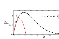
Figure 1: Average potential energy per particle as a function of an interaction strength for a homogenous system for $\rho_{b}\sigma^{3}=0.5$. Exact results are from the MC simulation for $N=1000$ particles. The RPA data points correspond to Eq. (19), and the mean-field result to the first term of that expression.

To understand the above results, in Fig. (2) we plot correlation functions which contribute to the behavior of $\beta E$. The RPA correlations are calculated numerically from

$$h(r)=-\bigg{(}\frac{1}{2\pi}\bigg{)}^{3}\int_{0}^{\infty}dk\,\frac{4\pi k^{2}\beta\tilde{u}(k)}{1+\beta\rho_{b}\tilde{u}(k)}\frac{\sin kr}{kr}.$$ (22)

For separations $r>\sigma$ the resulting correlations compare reasonably well with the exact results. However, it is correlations at separations less than $\sigma$ that determine $\beta E$, and here the RPA correlations fail.

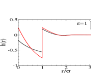
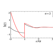
Figure 2: Pair correlation functions of a homogeneous fluid for $\rho_{b}\sigma^{3}=0.5$.

We next focus on a quantity $h^{\rm rpa}(0)$ as a function of $\alpha$ that determines $\beta E$ within the RPA (see Eq. (19)). The results are shown in Fig. (3) (a) and indicate a sharp increase of $h^{\rm rpa}(0)$ and then as $\alpha\to 34.81$, $h^{\rm rpa}(0)$ diverges.

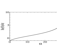
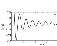
Figure 3: (a) The correlation function for a separation r = 0 as a function of $\alpha=4\pi\varepsilon\rho_{b}\sigma^{3}$. (b) The correlation function for ?? near the point of divergence.

Furthermore, the divergence is coextensive with the emergence of the solid like regular structure as shown in Fig. (b) and signaling the presence of an anomalous phase transition (anomalous because not predicted by simulations). The divergence occurs when the denominator in the expression for $\tilde{h}^{\rm rpa}(k)$ vanishes, which can only happen for negative $\tilde{u}(k)$. (For the Gaussian core model where $\beta\tilde{u}(k)=\pi^{3/2}\varepsilon\sigma^{3}e^{-k^{2}\sigma^{2}/4}\geq 0$ the divergence never arises Lowen01 ).

For the final illustration of the performance of the RPA we calculate pressure with results shown in Fig. (4). Because pressure is related to a density at a contact with a planar wall, $\beta P=\rho(0)$, the results provide insight about inhomogeneous density. Within the RPA the pressure is given by

$$\frac{\beta P}{\rho_{b}}=1+\frac{\alpha}{6}+\frac{1}{2}\int_{0}^{1}d\lambda\,\frac{h_{b}^{\lambda}(0)-\lambda h_{b}(0)}{\lambda},$$ (23)

and is obtained from the free energy of a homogeneous system $P=-(\partial F/\partial V)_{T,N}$. The data points for pressure are generally more reliable than those for $\beta E$ in Fig. (1). The mean-field and the RPA, not designed to recover a correct dilute limit, should generally become more reliable for dense systems. Going from $\rho_{b}\sigma^{3}=0.1$ to $\rho_{b}\sigma^{3}=0.3$ there is some improvement, but as $\rho_{b}$ continues to increase, the reliability becomes limited by the presence of a singularity (or a solid like structure of correlations) at $\alpha_{c}\approx 34.81$. The presence of the anomalous transition, therefore, limits the application of the RPA for penetrable-spheres.

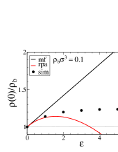
(a)  $\eta_{b}=0.1$

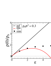
(b)  $\eta_{b}=0.3$

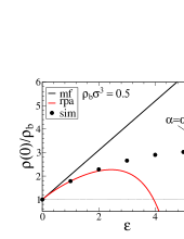
(c)  $\eta_{b}=0.5$

Figure 4: Density at a contact with a planar wall, $\rho(0)$, as a function of an interaction strength $\varepsilon$ for penetrable-spheres. The horizontal dotted line traces the ideal-gas behavior $\rho(0)/\rho_{b}=1$.

IV Planar wall confinment – an inhomogeneous case

In Fig. (5) we plot the entire density profile for a fluid confined by a hard wall at $x=0$. The two profiles correspond to $\rho_{b}\sigma^{3}=0.3$ and $0.5$, for the interaction strength $\varepsilon=3$. For $\varepsilon>3$ the RPA starts to break down, see Fig. (4). The RPA profile show decisive improvement in comparison to the bare mean-field.

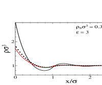
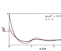
Figure 5: Density profiles for penetrable-spheres confined by a wall at $x=0$.

Another quantity that offers a test of performance is the excess adsorption defined as

$$\Gamma=\int_{0}^{\infty}dx\,\Big{[}\rho(x)-\rho_{b}\Big{]}.$$ (24)

Unlike the contact density that is related to properties within a bulk, there’s no equivalent relation available for the excess adsorption. $\Gamma$ is the surface quantity and as such is related to a surface tension $\gamma$, or more specifically to the derivative of the surface tension w.r.t. the chemical potential $\mu$,

$$\Gamma=-\bigg{(}\frac{\partial\gamma}{\partial\mu}\bigg{)}_{T,V},$$ (25)

according to the Gibbs adsorption theorem. In Fig. (6) we plot $\Gamma$ for a single density $\rho_{b}\sigma^{3}=0.5$. As for the contact density, the RPA undermines $\Gamma$ while the mean-field systematically overestimates it.

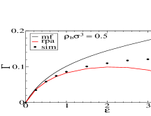
Figure 6: Excess adsorption defined in Eq. (24) as a function of $\varepsilon$ for penetrable-spheres near a hard-wall for the bulk density $\rho_{b}\sigma^{3}=0.5$.

V Alternative approaches

As the RPA applied to penetrable-spheres is unreliable both in the dilute limit (because of construction) and for large $\alpha$ (because of the emergence of a local solid-like structure for $\alpha\approx 34.81$), one may wish for an alternative approach. To speculate such an approach, it may be helpful to consider a virial expansion of the excess free energy,

$$F_{\rm ex} = \frac{1}{2}\int\!\!d{\bf r}_{1}\!\!\int\!\!d{\bf r}_{2}\,\rho({\bf r}_{1})\rho({\bf r}_{2})\bar{f}(r_{12})$$ (26)

$$+ \frac{1}{6}\int\!\!d{\bf r}_{1}\!\!\int\!\!d{\bf r}_{2}\!\!\int\!\!d{\bf r}_{3}\,\rho({\bf r}_{1})\rho({\bf r}_{2})\rho({\bf r}_{3})\bar{f}(r_{12})\bar{f}(r_{23})\bar{f}(r_{31})$$

$$+ \dots,$$

where $\bar{f}(r)=1-e^{-\beta u(r)}$ is the negative Mayer $f$-function, for penetrable-spheres given by $\bar{f}(r)=(1-e^{-\varepsilon})\Theta(\sigma-r)$. The excess free energy incorporates all the contributions due to particle interactions, $F_{\rm ex}=\frac{1}{2}\int d{\bf r}\int d{\bf r}^{\prime}\,\rho({\bf r})\rho({\bf r}^{\prime})u({\bf r},{\bf r}^{\prime})+F_{c}$. The two initial terms of the expansion have a simple ring topology. The higher order terms, however, become increasingly more complex, and the next term already involves three topologically distinct diagrams.

In the dilute limit the first term in Eq. (26) should generally suffice,

$$F_{\rm dil}=F_{\rm id}+\int d{\bf r}\,\rho({\bf r})U({\bf r})+\frac{1}{2}\int\!\!d{\bf r}_{1}\!\!\int\!\!d{\bf r}_{2}\,\rho({\bf r}_{1})\rho({\bf r}_{2})\bar{f}(r_{12}),$$ (27)

and the resulting expression structurally resembles the mean-field approximation in Eq. (1). However, different parametrization of the two approaches corresponds to different limits. Within the dilute limit approximation the pressure becomes

$$\frac{\beta P}{\rho_{b}}=1+\frac{4\pi\rho_{b}\sigma^{3}(1-e^{-\varepsilon})}{6}.$$ (28)

In Fig. (7) we compare the above expression with the mean-field, the RPA, and the exact data points. The dilute limit approach systematically underestimates particle interactions and performs poorly for higher densities.

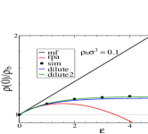
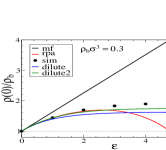
Figure 7: Density at a contact with a planar wall, $\rho(0)$, as a function of an interaction strength $\varepsilon$ for penetrable-spheres. The results labeled as ”dilute” correspond to Eq. (28).

Consecutive addition of terms of the virial expansion can correct the dilute limit predictions up to some point, but a truncated series will always diverge at a sufficiently high density. Instead of such a simple truncation, a ”wiser” approach is to selectively include/exclude entire classes of diagrams. Such a selection is naturally achieved by an application of more advanced closures, for example the Percus-Yevick or the hypernetted chain approximation. However, when combined with the adiabatic connection framework, Eq. (5) and Eq. (6), these closures introduce another level of complexity as the functional derivative $\frac{\delta F_{\rm ex}}{\delta\rho}$ involves an integral over $\lambda$, and to calculate a density, correlations for all values of $\lambda$, from $0$ to $1$, are needed. This difficulty precludes these approaches from having practical use.

To take a different approach, we take advantage of the RPA mathematical framework which is, as said before, defined in terms of integrals with ring topology. Defining the operator $B({\bf r},{\bf r}^{\prime})=\rho({\bf r})\bar{f}({\bf r},{\bf r}^{\prime})$ and using conventions of the linear algebra, all the ring terms of the excess free energy can be represented as

$$F_{\rm ex}^{\rm dil2}[\rho] = \frac{1}{2}\int d{\bf r}\int d{\bf r}^{\prime}\,\rho({\bf r})\rho({\bf r}^{\prime})\bigg{[}\bar{f}({\bf r},{\bf r}^{\prime})+\frac{\bar{f}^{2}({\bf r},{\bf r}^{\prime})}{2}\bigg{]}$$ (29)

$$+ \frac{1}{2}{\rm Tr}\bigg{[}\log(I+B)-B\bigg{]}.$$

We compare this with the RPA excess free energy given by

$$F_{\rm ex}^{\rm rpa}[\rho] = \frac{1}{2}\int d{\bf r}\int d{\bf r}^{\prime}\,\rho({\bf r})\rho({\bf r}^{\prime})u({\bf r},{\bf r}^{\prime})$$ (30)

$$+ \frac{1}{2}{\rm Tr}\bigg{[}\log(I+A)-A\bigg{]},$$

where $A({\bf r},{\bf r}^{\prime})=\rho({\bf r})u({\bf r},{\bf r}^{\prime})$. There are two main differences between the two expressions. First, $u({\bf r},{\bf r}^{\prime})$ is substituted by $\bar{f}({\bf r},{\bf r}^{\prime})$. Second, the ”mean-field” part involves an extra term. In Fig. (7) we plot the pressure data points from this new scheme labeled as ”dilute2”. There is a slight improvement over the results in Eq. (28), but taking into account the additional complexity, the improvement does not justify the approach. It becomes clear that terms with more complex topology are necessary for an accurate description of dense fluids.

VI Two-component system

In this section we consider a two-component system with symmetric interactions defined as follows: particles of the same species interact as $u(r<\sigma)=\varepsilon$, and particles of different species interact as $u(r<\sigma)=-\varepsilon$, in both cases $u(r>\sigma)=0$. This is an interesting scenario because all the mean-field contributions cancel out and interactions are captured only through correlational contributions.

The present system gives rise to four different correlations, $h_{11}({\bf r},{\bf r}^{\prime}),h_{22}({\bf r},{\bf r}^{\prime}),h_{12}({\bf r},{\bf r}^{\prime}),h_{21}({\bf r},{\bf r}^{\prime})$, where $1$ and $2$ designate two species. By virtue of the symmetry of the interactions $h_{11}({\bf r},{\bf r}^{\prime})=h_{22}({\bf r},{\bf r}^{\prime})$ and $h_{12}({\bf r},{\bf r}^{\prime})=h_{21}({\bf r},{\bf r}^{\prime})$. Furthermore, within the RPA $h_{11}({\bf r},{\bf r}^{\prime})=-h_{21}({\bf r},{\bf r}^{\prime})$, $h_{22}({\bf r},{\bf r}^{\prime})=-h_{21}({\bf r},{\bf r}^{\prime})$, and so forth, so that all correlations may be represented by a single functional form $h({\bf r},{\bf r}^{\prime})$ obtained from the OZ relation

$$h({\bf r},{\bf r}^{\prime})=-\beta u({\bf r},{\bf r}^{\prime})-\beta\!\!\int\!\!d{\bf r}^{\prime\prime}\rho({\bf r}^{\prime\prime})h({\bf r}^{\prime},{\bf r}^{\prime\prime})u({\bf r},{\bf r}^{\prime\prime}),$$ (31)

where $\rho({\bf r})=\rho_{1}({\bf r})+\rho_{2}({\bf r})$ is the total number density, $h_{11}({\bf r},{\bf r}^{\prime})=h({\bf r},{\bf r}^{\prime})$, $h_{12}({\bf r},{\bf r}^{\prime})=-h({\bf r},{\bf r}^{\prime})$, and so forth. Now, if such a two-component fluid is constrained to a half-space $x>0$ by a planar wall, a number density for a species $i$ is given by

$$\rho_{i}({\bf r})=\frac{\rho_{b}}{2}e^{\frac{1}{2}[h({\bf r},{\bf r})-h_{b}(0)]},$$ (32)

where $\rho_{b}$ is the total bulk density. Note that the mean-field contributions are absent and the density is determined solely by correlations.

Considering a homogeneous fluid, an average potential energy that a particle of the species $1$ feel is

$$\beta E=\frac{\varepsilon\rho_{b}}{2}\int_{0}^{\sigma}dr\,r^{2}\big{[}h_{11}(r)-h_{12}(r)\big{]}.$$ (33)

Within the RPA the above expression can be written as

$$\beta E^{\rm rpa}=-h_{b}^{\rm rpa}(0)-\varepsilon.$$ (34)

Fig. (8) shows $\beta E$ as a function of $\varepsilon$ for $\rho_{b}\sigma^{3}=0.5$. Within the range $\varepsilon<1$ the RPA data points are highly accurate.

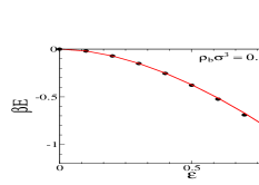
Figure 8: Average potential energy per particle as a function of $\varepsilon$ for a homogenous two-component system with total density $\rho_{b}\sigma^{3}=0.5$. The RPA result corresponds to Eq. (34). There are no mean-field contributions.

The fact that $\beta E$ monotonically decreases with increasing $\varepsilon$ indicates increased association between particles of different species, which eventually leads to phase-transition around $\varepsilon=1$. For illustration in Fig. (9) we show a configuration snapshot of a two-component system in 2D after phase transition where the system consists of highly structured clusters. The RPA does not indicate any phase transition around this point.

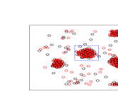
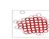
Figure 9: Configurational snapshots of a two-component penetrable-sphere system, after the phase transition. For the sake of simplicity the snapshots are for a 2D system. The red and black circles indicate particles of different species. The system parameters are $\varepsilon=1$ and $\rho_{b}\sigma^{2}=0.9$. The first figure contains $N=1000$ particles and the second one $N=240$.

In Fig. (10) we look into correlations $h_{11}(r)$ and $h_{12}(r)$, which reveal that the RPA correlations are not at all that accurate.

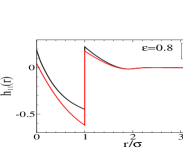
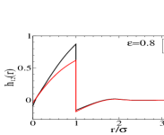
Figure 10: Pair correlation functions of a homogeneous two-component fluid for $\rho_{b}\sigma^{3}=0.5$. By virtue of symmetric interactions, $h_{11}({\bf r},{\bf r}^{\prime})=h_{22}({\bf r},{\bf r}^{\prime})$ and $h_{12}({\bf r},{\bf r}^{\prime})=h_{21}({\bf r},{\bf r}^{\prime})$.

From Eq. (33) we know, however, that $\beta E$ depends on the quantity $h_{11}(r)-h_{12}(r)$ (within the RPA given by $2h(r)$). Accordingly, in Fig. (11) we plot $h_{11}(r)-h_{12}(r)$. Here the agreement between the simulation and the RPA is quite impressive and indicates some cancellation of errors, accrued in both $h_{11}(r)$ and $h_{12}(r)$, that is responsible for good results seen in Fig. (8).

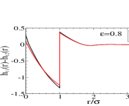
Figure 11: Correlations $h_{11}(r)-h_{12}(r)$ of a homogeneous fluid for $\rho_{b}\sigma^{3}=0.5$. Compare with Fig. (10) to understand the cancellation of errors in $h_{11}(r)$ and $h_{12}(r)$.

Next we calculate the pressure, within the RPA given by

$$\frac{\beta P}{\rho_{b}}=1+\frac{1}{2}\int_{0}^{1}d\lambda\,\bigg{(}\frac{h_{b}^{\lambda}(0)-\lambda h_{b}(0)}{\lambda}\bigg{)}.$$ (35)

where

$$h_{\lambda}^{\rm rpa}({\bf r},{\bf r}^{\prime})=-\lambda\beta u({\bf r},{\bf r}^{\prime})-\lambda\beta\!\!\int\!\!d{\bf r}^{\prime\prime}\rho({\bf r}^{\prime\prime})h^{\rm rpa}_{\lambda}({\bf r}^{\prime},{\bf r}^{\prime\prime})u({\bf r},{\bf r}^{\prime\prime}),$$ (36)

The expression for pressure is similar to that in Eq. (23) without the mean-field term. The results are plotted in Fig. (12). Once again, the agreement between the simulation and the RPA is quite excellent.

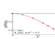
Figure 12: Density at a contact with a planar wall, $\rho(0)=\rho_{1}(0)+\rho_{2}(0)$, as a function of an interaction strength $\varepsilon$.

Finally, in Fig. (13) we plot the entire density profiles for penetrable-spheres confined by a wall at $x=0$. The RPA for this situation once again turns out being very accurate.

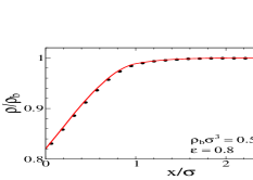
Figure 13: Density profile for two-component penetrable-spheres near a planar wall at $x=0$.

VII Conclusion

The main lesson to be taken from this study is that the RPA, despite its non-perturbative construction, is not a theory of the strong-coupling regime. The RPA introduces correlations to the mean-field level of description, but does not really extend the range of validity of the mean-field. The RPA is shown to be especially useful for situations in which the mean-field contributions are cancelled, as in the case of a two-component system considered in the present study. The RPA for this situation is found to be rather accurate, albeit within the weak-coupling limit, while the cause of this success lies in a somewhat lucky cancellation of errors.

- (1) D. Frydel and M. Ma, Phys. Rev. E 93, 062112 (2016).
- (2) D. Frydel, Adv. Chem. Phys. 160, 209 (2016).
- (3) R. R. Netz and H. Orland, Europhys. J. E 1, 67 (2000).
- (4) Z.-G Wang, Phys. Rev. E 81, 021501 (2010).
- (5) Zhenli Xu, A. C. Maggs, J. Comp. Phys. 275, 310 (2014).
- (6) T. Markovich, D. Andelman and R. Podgornik, Eur. Phys. Lett. 106, 19903 (2014).
- (7) D. Frydel, Eur. J. Phys. 36, 065050 (2015).
- (8) X. Ren, P. Rinke, C. Joas, M. Scheffler, J. Mater. Sci. 47, 7447 (2012).
- (9) J. P. Hansen and I. R. McDonald, Theory of Simple Fluids (London: Academic, 2005).
- (10) A. A. Louis, P. G. Bolhuis, J. P. Hansen, and E. J. Meijer, Phys. Rev. Lett. 85, 2522 (2000).
- (11) A. J. Archer and R. Evans, Phys. Rev. E 64, 041501 (2001).
- (12) D. Frydel, J. Chem. Phys. 145, 184703 (2016).
- (13) C. N. Likos, A. Lang, M. Watzlawek, and H. Löwen Phys. Rev. E 63, 031206 (2001).