Non-equilibrium transitions in multiscale systems with a bifurcating slow manifold

Abstract

Noise-induced transitions between metastable fixed points in systems evolving on multiple time scales are analyzed in situations where the time scale separation gives rise to a slow manifold with bifurcation. This analysis is performed within the realm of large deviation theory. It is shown that these non-equilibrium transitions make use of a reaction channel created by the bifurcation structure of the slow manifold, leading to vastly increased transition rates. Several examples are used to illustrate these findings, including an insect outbreak model, a system modeling phase separation in the presence of evaporation, and a system modeling transitions in active matter self-assembly. The last example involves a spatially extended system modeled by a stochastic partial differential equation.

1 Introduction

Systems in nature are commonly found to evolve on multiple time scales. One typically distinguishes slow variables $x\in\mathbb{R}^{n}$, that change on a time scale slow compared to the fast variables $y\in\mathbb{R}^{m}$. In a traditional setup [1, 2], these systems can be written as ODEs of the form

$$\dot{x} =\alpha u(x,y)$$ (1)

$$\dot{y} =v(x,y)\,.$$

where the parameter $\alpha$ measures how fast the variables $y$ evolve compared to $x$. In the limit $\alpha\to 0$ when the time scale separation becomes infinite, some concepts are commonly defined for slow-fast systems of the above form, in particular:

• the system may converge to a slow manifold $\mathcal{M}$ where $v(x,y)=0$ on the fast scale, so that the dynamics, after a short transient, are reduced to a movement closely along this manifold, and;

• changes in stability along the slow manifold may lead to bifurcation, with the slow variables playing the role of control parameters.

On top of the deterministic dynamics of (1), both the slow and the fast variables in many realistic systems are subject to small intrinsic stochastic fluctuations, for example due to thermal noise, or the discreteness of an underlying microscopic model. These fluctuations introduce another time scale: the system may be confined in a metastable region of the slow-fast dynamics for long periods of time and only rarely switches between different such regions. Specifically, in the case where the deterministic dynamics of (1) permit multiple locally stable fixed points $(x_{i},y_{i})$ such that $u(x_{i},y_{i})=v(x_{i},y_{i})=0$, small fluctuations of order $\mathcal{O}(\epsilon)$ may push the system from the vicinity of one stable fixed-point to another. On time scales larger than the Kramers’ time, which is typically $\mathcal{O}(\exp(\epsilon^{-1}))$, these transitions become almost certain, and are captured precisely by large deviation theory (LDT) [3]. On these time scales, the dynamics can then be effectively reduced to that of a Markov jump process on the metastable states [3, 1]. In the present paper, our aim is to analyze how the slow-fast nature of the dynamics and its associated bifurcation structure influence the pathways of the noise-induced transitions between metastable fixed-points. We will focus mostly on situations where the Kramers’ time is the longest time scale of the system. The presence of three time scales in interaction with the bifurcation structure quickly leads to a rich set of possible phenomena. The objective of this paper is to identify common patterns in these situations and apply them to specific applications as a first step towards an exhaustive theory. Our main contribution is to elucidate the role of the bifurcation structure of the slow-fast time scale separation on metastability. Interesting phenomena also occur in regimes where the Kramers’ time is between slow and fast time scales [4, 1, 2], like for example in the context of coherent or stochastic resonance phenomena [5, 6, 7, 8, 9]. Similarly, one can consider the case where the large deviation smallness parameter $\epsilon$ is the time scale separation $\alpha$ itself [10, 11, 12, 13]. These situations are not considered here.

The remainder of this paper is organized as follows. In Section 2 we present the type of fast slow system we will study and discuss their slow manifold and bifurcation structures. We also introduce the effect of fluctuations on the dynamics, leading to noise induced transitions between metastable fixed points captured by LDT. Some generic cases are analyzed explicitly in Section 3. In Section 4, we illustrate the theory for several finite dimensional applications that cover different bifurcation structures, including a model for insect outbreak in Section 4.1 and a model for phase separation in the presence of evaporation in Section 4.2. The generalization to infinite dimensional applications is presented in Section 5, where the theory is applied to a stochastic partial differential equation modeling motility induced phase separation for motile microorganisms. The appendix covers details concerning the numerical computation of the most likely transition pathway in A and of the bifurcation structure in B.

2 Problem set-up and phenomenology

2.1 Bifurcation and control parameter

We are going to use a generalized form of the system (1) that describes the evolution of a single variable $z\in\mathbb{R}^{d}$ obeying

$$\dot{z}=f(z)+\alpha g(z)$$ (2)

where $f(z)$ describes the fast dynamics and $g(z)$ the slow dynamics, and the time scale separation is measured by $\alpha\ll 1$. All systems of type (1) can be brought into this form by taking $z=(x,y)$, but in general for equation (2), it is not clear a priori what the slow and fast variables are (as they are not necessarily isolated components of $z$). We call the set

$$\mathcal{M}=\{v\in\mathbb{R}^{d}|f(v)=0\}$$ (3)

the slow manifold of the system (2), to which the system converges via the fast dynamics $\dot{z}=f(z)$ when we take $\alpha\ll 0$. In other words, the fixed points of the fast dynamics make up the slow manifold $\mathcal{M}$. The slow manifold is comprised of stable branches, i.e. sets of points $v\in\mathcal{M}$ for which $\nabla f(v)$ has eigenvalues with negative real part only, as well as unstable branches, where at least one eigenvalue has a positive real part.

We call slow variables all quantities left invariant on the fast time scale, i.e. slow variables are conserved quantities of the fast dynamics. Dynamics on the slow time scale are described by the reduced dynamics defined by the projection of the slow dynamics into the tangent space of the slow manifold.

Furthermore, we can identify all points on the slow manifold by the associated values of the slow variables. In other words, the slow manifold is foliated by the slow variables. As a consequence, it makes sense to use the slow variables as control parameters $\mu$ for a bifurcation analysis. Varying the control parameter, branches of the slow manifold appear or disappear, split or merge. The points $v\in\mathcal{M}$ where this happens are called bifurcation points, which are equivalent to points where the stability of the slow manifold changes.

Note that all above definitions solely reference the fast dynamics $f(z)$, regardless of the choice of $g(z)$. For small but finite time scale separation $\alpha$, the picture is necessarily perturbed: The reduced dynamics do not track the slow manifold exactly, changes of stability do not occur exactly at bifurcation point, etc.

2.2 Noise-induced transitions

We now want to introduce stochastic fluctuations to the slow-fast system (2), by taking

$$dZ=(f(Z)+\alpha g(Z))\,dt+\sqrt{\epsilon}\sigma dW\,.$$ (4)

Here, $\epsilon$ is a parameter that will be considered small (as we are interested in the low noise regime), $\sigma\in\mathbb{R}^{d\times d}$ is the noise correlation matrix and $W$ is a Wiener process (Brownian motion). The noise term is to be understood as the combined effect of all fluctuations of the system, and is assumed to be Gaussian. In principle, if we assume slow and fast dynamics to be induced by two separate physical mechanisms, each might be attained with its own intrinsic fluctuations, acting on different time scales, with different correlations, possibly degenerate and possibly non-Gaussian. We will consider situations of this type later, but for time being focus on the cases where the effect of the noise can be combined as in equation (4) with $\sigma\sigma^{T}$ invertible (i.e. the diffusion (4) is elliptic) and $\sigma$ is independent of $\alpha$. In the small noise limit, $\epsilon\to 0$, we will start the discussion with systems that have only two distinct deterministically stable fixed points $z_{A}$ and $z_{B}$. The same arguments can be applied to any pair of an arbitrary higher number of stable fixed points (for more generic attractors, such as limit cycles, the situation becomes more complicated). Limiting ourselves to two stable fixed points $z_{A}$ and $z_{B}$, we are interested in the noise-induced transitions between them. For deterministic dynamics, $\epsilon=0$, each of the stable fixed points is surrounded by its respective basin of attraction,

$$\mathcal{B}_{i}=\left\{z\in\mathbb{R}^{d}\,\Big{|}\,\lim_{t\to\infty}\left|z(t)-z_{i}\right|=0\text{ for }\epsilon=0\text{ if }z(0)=z\right\}\,,\qquad i=A,B\,,$$ (5)

so that all deterministic trajectories that are initially located in $\mathcal{B}_{i}$ will converge arbitrarily close to $z_{i}$ for large times. The two basins are separated by a separatrix, which, in the simplest case, contains a single saddle point $z_{S}$, i.e. a fixed point where one eigenvalue of $\nabla(f(z_{S})+\alpha g(z_{S}))$ is negative, while all others have a positive real part.

Adding fluctuations, the generic picture of the low-noise limit implies that, after an initial transient, the system spends most of its time close to one of the stable fixed points. Only rarely excursions occur that push the state over the separatrix into the other basin of attraction, where it will deterministically converge close to the other deterministically stable fixed point. In the limit $\epsilon\to 0$ these transitions can be described precisely by Freidlin-Wentzell theory of large deviations [3]: To compute the most probable transition pathway for a transition time $T$, we find the trajectory $z$ whose Freidlin-Wentzell action or rate function

$$S^{\alpha}_{T}(z)=\frac{1}{2}\int_{0}^{T}\left|\sigma^{-1}\left(\dot{z}-f(z)-\alpha g(z)\right)\right|^{2}\,dt$$ (6)

is minimal. Since in general $T$ is not prescribed and we want to find the most probable transition for an arbitrary transition time, we look at the double minimization

$$\inf_{T>0}\inf_{z}S^{\alpha}_{T}(z)\,.$$ (7)

Typically, since we are starting from (and ending at) a stable fixed point, the minimum will be achieved when $T\to\infty$, meaning that (7) has no minimizer unless we reparametrize it in time: understanding the minimizer in this general sense, we will denote it by $z^{\star}$, and refer to it as the maximum likelihood transition pathway (MLP) or instanton.

In the gradient case, and with $\sigma=\sqrt{2}\,\text{\it Id}$, the system (4) is in detailed balance, and there exists a potential or free energy $U_{\alpha}:\mathbb{R}^{d}\to\mathbb{R}$ such that $f(z)+\alpha g(z)=-\nabla U_{\alpha}(z)\,\forall\,z\in\mathbb{R}^{d}$. This assumption significantly simplifies the large deviation computation. In particular, the ‘uphill” portion of the transition (i.e. the portion where fluctuations are necessary to overcome the deterministic dynamics), fulfills

$$\frac{1}{4}\int_{0}^{T}|\dot{z}+\nabla U_{\alpha}(z)|\,dt=\frac{1}{4}\int_{0}^{T}|\dot{z}-\nabla U_{\alpha}(z)|\,dt+(U_{\alpha}(z(T))-U_{\alpha}(z(0)))\,,$$ (8)

which is minimized by $\dot{z}^{\star}=\nabla U_{\alpha}(z^{\star})$. The rate function is therefore equal to the barrier height $U_{\alpha}(z(T))-U_{\alpha}(z(0))$ along the MLP. As a direct consequence, the MLP crosses the separatrix at the saddle point $z_{S}$, where the barrier is lowest, i.e. the barrier height corresponds to the potential difference between the fixed point $z_{A}$ and the saddle point $z_{S}$. Furthermore, since for all $t$, $\dot{z}^{\star}(t)$ is parallel to $\nabla U_{\alpha}(z^{\star}(t))$, the MLP coincides with the heteroclinic orbits (HO) connecting $z_{S}$ to $z_{A}$ and $z_{B}$. Note also that this implies that forward and backward transitions follow the same path in reverse. Indeed the “uphill” portion obeys exactly the time-reversed dynamics of the “downhill” portion, which is a direct consequence of the detailed balance property that holds in the equilibrium case.

In the non-equilibrium case, where detailed balance is broken and the HO no longer coincides with the MLP, in general we have to resort to numerical minimization of the action functional (6) to obtain the MLP. In the setup lined out above, though, it remains correct that once the MLP crosses the separatrix, it will obey the deterministic dynamics, and it will cross the separatrix at the saddle point $z_{S}$. On the other hand, it is no longer true that forward and backward transitions are simply time-reversed, and detailed balance is broken. Instead, forward and backward transitions typically form a “figure-eight” shape, where the parts $z_{A}\to z_{S}$ and $z_{S}\to z_{A}$ (resp. $z_{B}\to z_{S}$ and $z_{S}\to z_{B}$) occur along different paths, but both forward and backward transition meet at $z_{S}$. In this case, there still is merit in computing the heteroclinic orbit even in the non-equilibrium setup, as it will yield the saddle point and half of each transition. (This intuition breaks down as soon as there are several saddle points, or a more complicated fixed-point structure on the separatrix. It is then possible that forward and backward transition share none but their initial and final points.)

2.3 Transitions for large time scale separation

The interplay between the stochastic fluctuations and the time scale separation warrants a separate discussion. In the case of large time scale separation, $\alpha\ll 1$, the stable fixed points necessarily lie close to the slow manifold $\mathcal{M}$, since either $f(z_{i})$ and $g(z_{i})$ individually vanish for $i=A,B$, and therefore $z_{i}\in\mathcal{M}$, or they cancel each other, in which case $\min_{v\in\mathcal{M}}|z_{i}-v|=\mathcal{O}(\alpha)$. The same is true for all fixed points of the deterministic dynamics, including the saddle $z_{S}$. This is of particular importance, since it implies that in the limit $\alpha\to 0$ (a) the separatrix (locally) coincides with the slow manifold, and (b) the slow manifold is unstable around $z_{S}$. The situation becomes particularly interesting if the two deterministically stable fixed points $z_{A},z_{B}$ are connected by the slow manifold in the limit $\alpha\to 0$. The intuition then is that the slow manifold opens a reactive channel for the transition, which will be used by the maximum likelihood transition pathway. This is plausible, since the reduced dynamics along the slow manifold are of order $\mathcal{O}(\alpha)$ and therefore are much easier to overcome by random fluctuations than the $\mathcal{O}(1)$ dynamics elsewhere.

To be more precise, we can rescale the time variable in the action (6) to the slow time scale $\tau=\alpha t$ to obtain

$$\alpha^{-1}S^{\alpha}_{T^{\prime}/\alpha}(z)=\frac{1}{2}\int_{0}^{T^{\prime}}\left|\sigma^{-1}\left(\dot{z}-\alpha^{-1}f(z)-g(z)\right)\right|^{2}\,d\tau$$ (9)

where $T^{\prime}=\alpha T$. Considering the limit $\alpha\to 0$ at $T^{\prime}$ fixed, the contribution of the fast dynamics becomes unbounded as soon as the trajectory leaves the slow manifold, where $f=0$. Indeed given a trajectory $z$

$$\lim_{\alpha\to 0}\alpha^{-1}S^{\alpha}_{T^{\prime}/\alpha}(z)<\infty\quad\text{if and only if $z\in\mathcal{M}$}$$ (10)

From this statement it follows that any transition of the system (4) in the large deviation regime between metastable fixed points that are connected by the slow manifold $\mathcal{M}$ will reach a bifurcation point $z_{X}$ in the limit $\alpha\to 0$. This portion of the transition will be the only one that contributes to the action, while the motion after $z_{X}$ is deterministic.

Note though that the mode of descend from the bifurcation point $z_{X}$ onwards is nontrivial. Since the separatrix is unstable, the transition trajectory may leave it at any point up to the saddle, and deterministically relax into the opposing fixed point. The action attained along all of these trajectories is zero, but they each carry some probability current. A more refined estimate of the action than our approach above is necessary to analyze their relative weight. Note though that the leading scaling of the transition probability itself is unaffected by these complications. A more detailed analysis of similar setups is performed in the literature [14, 15]. For any finite but small value of $\alpha$, on the other hand, the separatrix has to be crossed precisely at the saddle $z_{S}$, but due to the scaling of the action (10) the slow manifold is still used as reactive channel. Since the slow manifold is locally stable around $z_{A}$ and $z_{B}$, and locally unstable around $z_{S}$, the MLP must also closely pass a bifurcation point $z_{X}$, where $\mathcal{M}$ changes stability. This implies the counter-intuitive fact that the MLP approaches the separatrix already at $z_{X}$, which is far from the saddle $z_{S}$, and then “skirts” the separatrix for an extended time quasi-deterministically into $z_{S}$. We will confirm this intuition in a number of examples below.

The setup lined out above, where the stable fixed points of a slow-fast system are connected by the slow manifold, turns out to be quite ubiquitous in nature, with applications in physics (active Brownian particles, active matter), chemistry (reaction-diffusion), and biology (motile microorganisms, chemotaxis, predator prey models). In the sequel, we will study several examples arising in these contexts. In particular we will discuss also an infinite dimensional example (that is, including a spatial dimension): Active particle phase separation, where the fast phase separation term is combined with a slow destabilizing term, a model also applicable to motile microorganisms with a fast propulsion and slow growth term.

2.4 The case with slow-fast noises

It is also useful to consider situations in which the fluctuations on the slow and fast variables act on their respective time scales, that is, models of the type

$$dX =\alpha u(X,Y)dt+\sqrt{\alpha\epsilon}\sigma_{x}dW_{x}$$ (11)

$$dY =v(X,Y)dt+\sqrt{\epsilon}\sigma_{y}dW_{y}\,.$$

where $W_{x}$ and $W_{y}$ are independent and both $\sigma_{x}\sigma_{x}^{T}$ and $\sigma_{y}\sigma_{y}^{T}$ are invertible and independent of $\alpha$. In this case, the Freidlin-Wentzell action reads

$$S^{\alpha}_{T}(x,y)=\frac{1}{2}\int_{0}^{T}\left(\alpha^{-1}\left|\sigma_{x}^{-1}\left(\dot{x}-\alpha u(x,y)\right)\right|^{2}+\left|\sigma_{y}^{-1}\left(\dot{y}-v(x,y)\right)\right|^{2}\right)\,dt$$ (12)

On the slow time scale $\tau=\alpha t$, this action can be equivalently written as

$$S^{\alpha}_{T^{\prime}/\alpha}(x,y)=\frac{1}{2}\int_{0}^{T^{\prime}}\left(\left|\sigma_{x}^{-1}\left(dx/d\tau-u(x,y)\right)\right|^{2}+\left|\sigma_{y}^{-1}\left(dy/d\tau-\alpha^{-1}v(x,y)\right)\right|^{2}\right)\,d\tau$$ (13)

These two expressions indicate that the action remains finite as $\alpha\to 0$ if it is evaluated on paths that either follow the slow manifold where $v(x,y)=0$ on the slow time scale, or take shortcuts at $x=cst$ (so that $\dot{x}=0$) on the fast time scale. This typically provides different possible scenarios for the transition, among which the most likely one (i.e. the one minimizing the action) will depend on the relative amplitude of $\sigma_{x}$ and $\sigma_{y}$. This will be illustrated via examples below.

Note that systems generalizing (11) are consistent with examples in which detailed balance is broken in a very specific way. Namely, situations where both fast and slow dynamics, taken by themselves, are in detailed balance with respect to their corresponding fluctuations, but in combination they are not. This setup is very natural: It occurs when both the slow and the fast term are modeling physical processes that are in detailed balance individually. In this case, the dynamics can be written as

$$dZ=-M_{1}\nabla E_{1}(Z)\,dt-\alpha M_{2}E_{2}(Z)\,dt+\sqrt{\epsilon_{1}}M_{1}^{1/2}\,dW_{1}+\sqrt{\alpha\epsilon_{2}}M_{2}^{1/2}\,dW_{2}$$ (14)

with free energies $E_{i}(z)$ and mobilities $M_{i}$, $i=1,2$. If the mobilities are incompatible, i.e. if one cannot find a single mobility $M$ such that the sum of the two gradient systems can be written as a single gradient with mobility $M$, then the system can no longer be in detailed balance, regardless of the choice of the noise correlation. The complete system then describes the competing influence of two distinct physical processes acting on different time scales. The incompatibility arises, for example, if one of the processes is conservative, (i.e. diffusion, advection, etc), while the other is not (i.e. evaporation, reaction, birth/death, etc). In this case, the conserved quantity also defines the slow variable and therefore the control parameter $\mu$ for the bifurcation. For example for conservative fast dynamics the control parameter is the spatial mean of the considered field variable. Both the finite dimensional phase separation/evaporation discussed in section 4.2 and the infinite dimensional Allen-Cahn/Cahn-Hilliard system discussed in section 5 are of this type for their deterministic dynamics, even though we simplified the noise terms in both cases.

2.5 Numerical aspects

Conducting the numerical minimization procedure is non-trivial due to the infinite time of the transition, $T=\infty$. We therefore use the simplified geometric minimum action method [16, 17], which harnesses the fact that the minimal action is invariant under reparametrization, and performs minimization in the space of arc-length parametrized curves instead. See A for details on the procedure. This computation is in contrast to the equilibrium setup, where the heteroclinic orbits describe the transition completely, and are efficiently computable by the string-method [18, 19]. Interestingly, the string method can still be used in the nonequilibrium context to identify the slow manifold $\mathcal{M}$ of the slow-fast system at hand, as outlined in B. It is important to note that our numerical method relies neither on the large time scale separation nor on the bifurcation structure of the system. Instead, it is applicable in general for the computation of any large deviation minimizer. This turns out to be of importance in applications, since this allows us to handle arbitrarily complicated bifurcation structures and small but finite values of $\alpha$, where the dynamics around bifurcation points and close to the slow manifold might become very complicated and might not be captured completely by the picture painted above. If anything, large values of time scale separation, $\alpha\ll 1$, are a numerical annoyance rather than help because of their associated stiffness.

3 Generic examples

3.1 Saddle-node bifurcation

Figure 1: Saddle-node bifurcation. Left: Bifurcation diagram with the slow variable as control parameter. At the bifurcation point $z_{X}={(-\tfrac{2}{9}\sqrt{3},\tfrac{1}{3}\sqrt{3})}$, a stable and an unstable branch of the slow manifold emerge. The MLP tracks the slow manifold into the saddle point. Right: The optimal jump location as a function of the relative noise strength $\beta$ in the limit $\alpha\to 0$.

The prototypical example of a bifurcation is the saddle-node bifurcation. In this section, we are going to construct a simple metastable system out of two of these. Consider the stochastic differential equation (SDE) for $z=(x,y)\in\mathbb{R}^{2}$ given by

$$dX =-\alpha Xdt+\sqrt{\alpha\epsilon}dW_{x}$$ (15)

$$dY =\left(Y-Y^{3}-X\right)dt+\sqrt{\beta\epsilon}dW_{y}\,.$$

Note that this is the case with slow-fast noise, in which the noise associated with the variables $X$ and $Y$ act on the slow and fast timescales, respectively, as in (11). Here we also took $\sigma_{x}=1$ and $\sigma_{y}=\beta$, which therefore quantifies the relative strength of the fluctuations on the slow and fast variables.

The deterministic system has two stable fixed points, which are located at $z_{A}=(0,1)$ and $z_{B}=(0,-1)$ and a saddle point at $z_{S}=(0,0)$. The $x$ component is invariant under the fast dynamics and is therefore a slowly evolving quantity. It foliates the slow manifold $\mathcal{M}$ and we can take it as the control parameter $\mu$ for a bifurcation analysis. The slow manifold $\mathcal{M}$ is comprised of all points $z_{\mathcal{M}}=(s-s^{3},s)$ with $s\in\mathbb{R}$, since $f(z_{\mathcal{M}})=0$. For large negative $\mu$, $\mathcal{M}$ has a single stable branch. Increasing $\mu$, a saddle-node bifurcation occurs at the point $z_{X}={(-\tfrac{2}{9}\sqrt{3},\tfrac{1}{3}\sqrt{3})}$, where another pair of branches emerge, one stable and one unstable. The unstable branch then disappears for positive $\mu$ in exactly the same way, leaving only a single stable branch for large values of $\mu$.

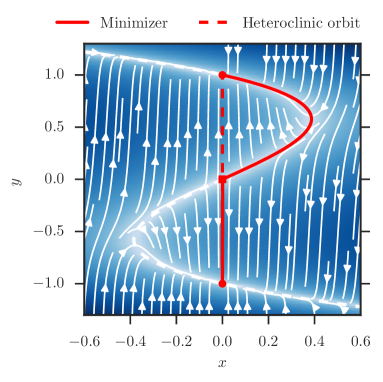
This system violates detailed balance and is not of gradient type, and therefore forward- and backward transitions between the stable fixed points $z_{A}$ and $z_{B}$ will not occur along the same trajectory. Both $z_{A}$ and $z_{B}$ lie on the slow manifold $\mathcal{M}$, and $\mathcal{M}$ connects both fixed points. It therefore seems intuitive that, in the small noise limit, $\epsilon\to 0$, the transition trajectory approaches the separatrix along the slow manifold, on which the drift has amplitude $\mathcal{O}(\alpha)$, and is therefore easier to overcome. This intuitive picture is confirmed in Fig. 1 (left): Here, the deterministic dynamics are depicted by the streamlines and their magnitude by the background shading. The two stable fixed points are marked by points, and the saddle by a square. The heteroclinic orbit connecting the saddle to the fixed points necessarily is a straight line, represented by the dashed line. The maximum likelihood transition pathway on the other hand uses the slow manifold as a transition channel, and therefore tracks $\mathcal{M}$ very closely from $z_{A}$ to $z_{S}$. It approaches the separatrix between the two basins of attraction at the bifurcation point $z_{X}$, and henceforth nearly deterministically tracks it to the saddle. Only subsequently does it follow the deterministic dynamics from the saddle onward.

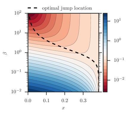
It is important to keep in mind that depending on the physical application the fluctuations associated with the reduced dynamics might be of order $\mathcal{O}(\sqrt{\alpha})$ (as assumed in this case). Then, even though the dynamics to overcome are weak in comparison to the fast dynamics, so is the noise term itself. In the limit $\alpha\to 0$, the transition can then be considered as arising from the combined effect of two distinct phenomena. The transition either tracks the slow manifold on the slow time scale, using the $\mathcal{O}(\sqrt{\alpha})$ fluctuations to overcome the $\mathcal{O}(\alpha)$ dynamics, or it can jump from one branch of the slow manifold to another, using the $O(1)$ fluctuations to overcome the $\mathcal{O}(1)$ fast dynamics. In the associated action, both contributions scale identically independently of $\alpha$, and the actual path of the transition has to be identified by minimization of this action. In general, the transition mechanism combines both effects: A migration along $\mathcal{M}$ until an optimal jump location is reached, and a subsequent jump from one branch to another, reaching the separatrix to the other basin.

The optimal jump location can then be identified explicitly in terms of $\beta$. Fig. 1 (right) shows the total action $S_{\mathcal{M}}+S_{\text{jump}}$ as a function of the jump location and $\beta$. The optimal jump location, where the minimum of the total action is reached, will vary in $\beta$, with an almost immediate jump at $\beta=10^{2}$, where the minimizer is basically identical to the heteroclinic orbit, to essentially no jump at all at $\beta=10^{-2}$. Fig. 1 (left) was obtained using $\beta=10^{-1}$.

One should keep in mind that these considerations are only relevant if the fluctuations of the reduced dynamics scale as $\mathcal{O}(\sqrt{\alpha})$. In what follows, with the exception of the insect outbreak model discussed in Sec. 4.1, a global $O(1)$ noise is assumed. In these cases, no jump can happen as $\alpha\to 0$, and the transition will track the slow manifold completely. In cases where part of the noise does scale $\mathcal{O}(\sqrt{\alpha})$, both the optimal jump location and the actual transition behavior for finite $\alpha$ usually have to be established using numerics, as done in this discussion.

The observed structure of the slow manifold $\mathcal{M}$ is re-occurring in different physical applications, including all applications discussed below: Two metastable fixed points are located on two distinct stable branches, separated by the unstable branch of $\mathcal{M}$, which coincides with the separatrix. Examples include the FitzHugh-Nagumo model [20, 21], which describes the excitability of the electrical potential across neural cell membranes in neural dynamics, and the more complicated Hodgin-Huxley [22] model.

3.2 Pitchfork bifurcation

Figure 2: Pitchfork bifurcation. Left: The MLP tracks the slow manifold into the bifurcation point $z_{X}=(-1,0)$, while the heteroclinic orbit leaves the slow variable $x$ unchanged. Right: Introducing a tilt $z_{\star}$ separates the bifurcation structure, breaking the symmetry in the relative stability of the two fixed points.

A pitchfork bifurcation is another example of a low-dimensional bifurcation structure. Consider for example the SDE for $z=(x,y)\in\mathbb{R}^{2}$ given by

$$dZ=f(Z)\,dt+\alpha g(Z)\,dt+\sqrt{\epsilon}dW\,,$$ (16)

with

$$f(z)=\left(\begin{matrix}0\\ -y\left(y^{2}-x-1\right)\end{matrix}\right)\,\qquad g(z)=-z\,.$$ (17)

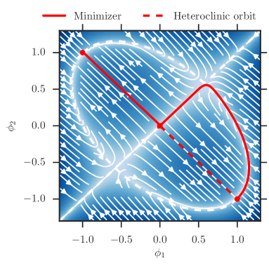
Again the system violates detailed balance and is not of gradient type. As before, $x$ is invariant under the fast dynamics and can be taken as bifurcation parameter $\mu$ that foliates the slow manifold $\mathcal{M}$. For large negative $\mu$, the system is only stable at $y=0$. If we increase the bifurcation parameter, a supercritical pitchfork bifurcation occurs at $\mu=-1$, where the single stable branch of $\mathcal{M}$ splits into two stable and one unstable branch. In (16) the noise is $\mathcal{O}(1)$ in $\alpha$, so that the MLP, in contrast to the heteroclinic orbit, utilizes the slow manifold for the transition. In particular, as depicted in Fig. 2 (left), it visits the bifurcation point $z_{X}=(-1,0)$ and approaches the separatrix before reaching the saddle point $z_{S}=(0,0)$.

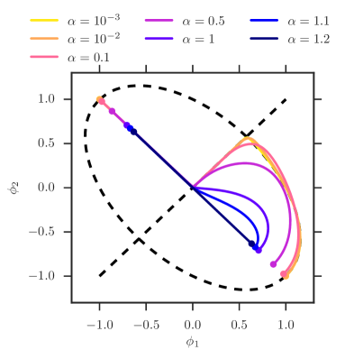
The situation becomes interesting if we introduce a tilt $z_{\star}$ to the slow term, i.e. choose $g(z)=z_{\star}-z$ instead of (17). Note that $g(z)$ modifies the drift of both $x$ and $y$, even though it acts on the slow time scale $\mathcal{O}(\alpha)$ only. In the limit $\alpha\to 0$, this tilt is therefore not felt, and the slow manifold $\mathcal{M}$ remains identical to the situation depicted in Fig. 2 (left). Nevertheless, for any finite choice of $\alpha$, this tilt will lead to a separation of the bifurcation structure and a breakdown of the pitchfork bifurcation to a mere saddle-node bifurcation. In particular, only one of the two separated components contains a bifurcation point and consequently only one transition direction can make full use of the slow manifold up to the saddle point, while the other has to bridge a gap. The corresponding transition trajectories are depicted in Fig. 2 (right), with the backward trajectory (solid) jumping from one part of the slow manifold to the other. In contrast, the forward transition (dashed) can follow the slow manifold completely to the bifurcation point and the saddle.

Even though the effect of the tilt is not felt as $\alpha\to 0$, it will have a dramatic effect for finite $\alpha$. For example, for the situation of Fig. 2 (right), $z_{\star}=(0,1)$ and $\alpha=10^{-2}$, but the ratio of the rates of forward and backward transition between $z_{A}$ and $z_{B}$ changes by roughly a factor $10^{5}$. An asymptotic analysis in $\alpha$ will be oblivious to this effect, which highlights the necessity to perform a numerical computation of the transition trajectory for practical applications.

4 Finite dimensional applications

4.1 Insect outbreak

Figure 3: Insect outbreak model, featuring a saddle-node bifurcation along the slow variable as control parameter. At the bifurcation point $z_{X}=(0.193,1.96)$, a stable and an unstable branch of the slow manifold emerge. The MLP tracks the slow manifold through the bifurcation point into the saddle point. Depicted are forward (left) and backward (right) transitions in comparison to the time reversible heteroclinic orbit.

A classical example of a slow-fast system from biology deals with outbreaks of the spruce budworm which attacks the leaves of the balsam fir tree. It was investigated extensively by Ludwig [23, 24] in the deterministic context, who modeled the interaction between the slowly recovering tree foliage area $X$ and the quickly reproducing budworm population $Y$. In a slightly modified form, and adding stochastic fluctuations to both degrees of freedom, we consider the system of SDEs

$$dX =\alpha X(1-X/x_{0})\,dt+\sqrt{\alpha\epsilon}\,dW_{x}$$ (18)

$$dY =Y(1-\frac{Y}{Xy_{0}})\,dt-\frac{Y^{2}}{X^{2}+Y^{2}}\,dt+\sqrt{\epsilon}\,dW_{y}\,.$$

Here, the tree foliage area $X$ recovers slowly on time scale $O(\alpha^{-1})$ to its long time limit $x_{0}$. In this simplified model, the foliage is not influenced by the budworm’s presence. For the normalized budworm population $Y$, the carrying capacity of their logistic growth, $Xy_{0}$, depends on the tree foliage area available. On top of that, budworms are subject to predation by birds, which is modeled by the second term in the equation for $Y$. It is chosen in a way that it saturates at high budworm densities due to e.g. territorial behavior of predators, but vanishes quadratically at low densities to model learning and reward mechanisms [23]. Both populations are subject to stochastic fluctuations, which are assumed to be Gaussian here for simplicity.

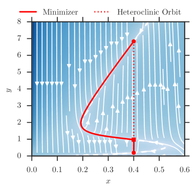
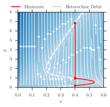
The SDE for $Z=(X,Y)\in\mathbb{R}^{2}$ is readily treated by the fast-slow formalism. The fast reproduction of the budworm (which can multiply five-fold in a single year [24]) occurs on a time scale of months, while the tree foliage area has a characteristic time scale of decades. The budworm population near instantaneously reacts to a change of the tree foliage area available; the resulting time scale separation gives raise to a slow manifold $\mathcal{M}$ foliated by the slow variable $x$, which is taken as control parameter $\mu$. In other words, for a given available tree foliage area $x$, the budworm population quickly adjusts to a compatible population density $y_{\mathcal{M}}(x)$, which will correspond to a point on a stable branch of $\mathcal{M}$ for this value of $x$. The tree foliage area only slowly changes, until a metastable fixed point is reached. Depending on the choice of parameters, the budworm/tree system may exhibit multiple metastable fixed points. For example for the choice $x_{0}=0.4$, $y_{0}=20$, $\alpha=10^{-2}$, two different configurations of tree foliage area and budworm density each are locally stable: $z_{A}=(0.4,6.83)$ and $z_{B}=(0.4,0.192)$, i.e. one configuration with a budworm outbreak, and one with a relatively low presence of budworms. Furthermore, there is a saddle point at $z_{S}=(0.4,0.974)$. The slow manifold $\mathcal{M}$ is comprised of all points $z_{\mathcal{M}}=(x,y_{\mathcal{M}}(x))$. For small values of $\mu$, $\mathcal{M}$ has a single stable branch. Increasing $\mu$, a saddle-node bifurcation occurs at the point $z_{X}=(0.193,1.96)$, where another pair of branches emerge, one stable and one unstable. The unstable branch then disappears for large $\mu$ in exactly the same way. The dynamics and the slow manifold $\mathcal{M}$ corresponding to this choice of parameters is depicted in Fig. 3, and are essentially those of the generic saddle-node example above.

The stable fixed points $z_{A},z_{B}$ lie on the slow manifold $\mathcal{M}$, and $\mathcal{M}$ connects both fixed points. Here, the maximum likelihood transition uses the slow manifold as a transition channel, and therefore tracks $\mathcal{M}$ very closely from $z_{A}$ to $z_{S}$. It approaches the separatrix between the two basins of attraction at the bifurcation point $z_{X}$, and henceforth nearly deterministically tracks it to the saddle. From the saddle onward, it follows the deterministic dynamics. Depicted are the transitions in both directions, $z_{A}\to z_{B}$ (left) and $z_{B}\to z_{A}$ (right). In both cases the conclusion is that a transition is most probable through slow fluctuations of the forest, instead of the insect population undergoing unusually large population fluctuations to overcome the barrier. This conclusion will no longer be true if either the fluctuations of the insect population are much bigger than those of the tree foliage area, or if the fluctuation strength becomes big enough for the Kramers’ time to be comparable to the slow time scale. In both these situations, the most likely transition will involve a fast portion, in which the path along the slow manifold is shortcut by a jump between branches of this slow manifold, as discussed in Sec. 3.2.

4.2 Phase separation with evaporation

Figure 4: Supercritical pitchfork bifurcation along the slow variable $\mu=\phi_{1}+\phi_{2}$. Left: At the bifurcation point $\phi_{X}=(-\sqrt{2/3},-\sqrt{2/3})$, the stable slow manifold splits into two stable and one unstable branch. The MLP tracks the slow manifold through the bifurcation point $\phi_{X}$ into the saddle at $\phi_{S}=(0,0)$. Right: Minimizers of the action functional (6) for model (21) for different values of $\alpha$. For $\alpha\to 0$, the transition happens increasingly close to $\mathcal{M}$.

The next example describes a situation where the time scale separation is introduced by two competing physical processes, namely phase separation and evaporation. We consider a simplified case with only two degrees of freedom, $\phi_{1}$ and $\phi_{2}$, which describe the concentration of some quantity relative to some reference density in two neighboring compartments. Phase separation is modeled by a free energy

$$E_{1}(\phi)=\tfrac{1}{4}\sum_{i=1}^{2}(1-\phi_{i}^{2})^{2}\,,$$ (19)

i.e. a double well potential, which is combined with a conservative mobility operator $M_{1}=Q=((1,-1),(-1,1))$, so that the mean $\phi_{1}+\phi_{2}$ is conserved, and the system tends to the two minima $(\pm 1,\mp 1)$. This situation corresponds to most of the mass being concentrated in either one of the two compartments, so that the respective densities are above the reference density in one and below the reference density in the other compartment. Evaporation is considered slow in comparison, and is modeled by a reversal of both degrees of freedom towards zero,

$$E_{2}(\phi)=\tfrac{1}{2}\sum_{i=1}^{2}\phi_{i}^{2}\,,$$ (20)

with a mobility $M_{2}=\alpha\,\textit{Id}$. This leads to a reversal of both densities towards the reference density, without necessarily preserving the mean. The two terms compete on different time scales. Due to the incompatibility of the mobility operators $M_{1}=Q$ and $M_{2}=\alpha\,\mathit{Id}$, detailed balance is broken and cannot be restored regardless of the choice of noise correlation. In total, we can write the system as the SDE

$$d\phi_{i}=\left(\sum_{j=1}^{2}Q_{ij}(\phi_{j}-\phi_{j}^{3})-\alpha\phi_{i}\right)dt+\sqrt{\epsilon}dW_{i}$$ (21)

with $\phi=(\phi_{1},\phi_{2})$, and where we assumed a Gaussian noise on all degrees of freedom, i.e. dropping the noise associated with $E_{1}$, $M_{1}$.

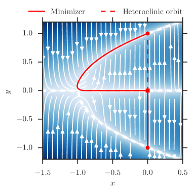
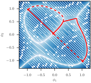
The dynamics of this model are depicted in Fig. 4 (left): The streamlines describe the direction of the deterministic dynamics, the shading its magnitude. The two stable fixed points fulfill $\lim_{\alpha\to 0}\phi_{A}=(-1,1)$ and $\lim_{\alpha\to 0}\phi_{B}=(1,-1)$ and are separated by the separatrix $\phi_{1}=\phi_{2}$, the point $\phi_{S}=(0,0)$ is a saddle point. In this case, the quantity $\mu=\phi_{1}+\phi_{2}$ remains unchanged under the fast dynamics. It is therefore a slow quantity and is chosen to be our control parameter. The slow manifold is comprised of all points where the fast dynamics $Q(\phi-\phi^{3})$ vanish. For large negative values of $\mu$, this happens only on the straight line where $\phi_{1}=\phi_{2}$, which is stable under the fast dynamics. The stability of the slow manifold changes at $\mu=-\sqrt{1/3}$ and undergoes a supercritical pitchfork bifurcation. The straight portion $\phi_{1}=\phi_{2}$ becomes unstable, and two new stable branches form a tilted ellipse $3(\phi_{1}+\phi_{2})^{2}+(\phi_{1}-\phi_{2})^{2}=4$. The same process occurs in reverse for $\mu>0$, where stability of $\phi_{1}=\phi_{2}$ is reinstated at $\mu=\sqrt{1/3}$. The complete slow manifold is depicted as a white dashed line.

Figure 5: Left: Action density for the supercritical pitchfork bifurcation model. The path parameter is normalized to $s\in(0,1)$. The action is $\mathcal{O}(\alpha)$ smaller for the large deviation minimizer. Right: Multiple transition trajectories obtained through direct sampling: The large deviation minimizer is followed up to the separatrix. The typical transition trajectory differs from the large deviation prediction from then on. Notably, almost no transition sample visits the transition state/saddle point in the center.

For model (21), the minimizer is depicted by the red solid line in Fig. 4. As the minimizer indeed follows the slow manifold, it approaches the separatrix at the bifurcation point $\phi_{X}$, far from the saddle-point $\phi_{S}$. It then tracks the separatrix quasi-deterministically into the saddle-point to cross into the other basin of attraction and then relax (deterministically) into the other fixed point. This is in contrast to the heteroclinic orbit connecting the two fixed points, which is the straight line through $\phi_{A}$ to $\phi_{B}$.

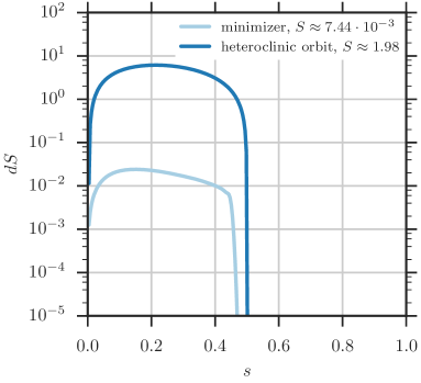
In the limit $\alpha\to 0$ indeed we confirm numerically that the transition trajectory for model (21) approaches the slow manifold. This fact is demonstrated in Fig. 4 (right). Note also that the switch to a straight line minimizer happens at a finite value $\alpha_{c}\approx 1.12$, i.e. there is no continuous straightening of the minimizer for growing $\alpha$, but a transition at a fixed critical $\alpha=\alpha_{c}$. The action along the minimizer and the heteroclinic orbit are depicted in Fig. 5 (left). Notably, due to its movement along the slow manifold, the action along the minimizer is smaller by a factor $\mathcal{O}(\alpha)$ than the action density along the heteroclinic orbit. This implies an exponentially larger transition probability along $\mathcal{M}$.

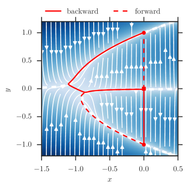
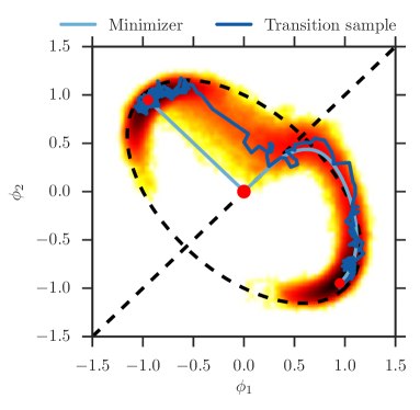
Due to the presence of the slow manifold for $\alpha\ll 1$, the noise-induced transition will approach the separatrix between the basins of attraction of the two stable fixed points not at the saddle point, but on the bifurcation point. Note that even though in the small noise limit $\epsilon\to 0$ the saddle point is visited subsequently as well, this is no longer true for any finite noise. In the presence of small but finite fluctuations, the typical transition trajectory will take a rather different trajectory due to the fact that the slow manifold becomes unstable after the bifurcation point. Fig. 5 (right) depicts this effect. Shown are the large deviation minimizer and a transition sample obtained by directly simulating the SDE (21) with finite noise. The background shading indicates the probability density for visiting each point conditioned on a transition happening. The transition samples follow closely the minimizer and the slow manifold up to the bifurcation point, but subsequently fall of the separatrix before reaching the saddle point in the center. These entropic effects imply that only the piece of the transition trajectory obtained through large deviation theory that requires the noise is observed in practice. Still, both the transition probabilities and the mean first passage times predicted by large deviation arguments remain correct. As the transition behind the bifurcation point is effectively deterministic, the minimum of the large deviation rate function is not changed by these modified transition trajectories.

4.3 Tilted phase separation

Figure 6: Inhomogeneous tilt $\phi_{\star}=(0.1,-0.1)$. Left: Forward and backward reaction differ, the slow manifold becomes disconnected. Right: Action density for the corresponding forward and backward reaction, logarithmic in $dS$. The jump from one slow manifold to the other is clearly visible as peak in the backward action. The forward action is order $O(\alpha)$ lower.

Consider a modification of (21) where we tilt the $E_{2}$ potential to break the symmetry between forward and backward reaction,

$$d\phi=\left(Q(\phi-\phi^{3})-\alpha(\phi-\phi_{\star})\right)dt+\sqrt{\epsilon}dW$$ (22)

where $\phi_{\star}$ defines the tilt. An homogeneous tilt (i.e. $\phi_{\star,1}=\phi_{\star,2}$) does not change the relative stability of the fixed points, since the system is still symmetric under reflection at the separatrix $\phi_{1}=\phi_{2}$. This is no longer true if we tilt orthogonal to the separatrix, as depicted in Fig. 6 (left). Here, forward and backward transition necessarily differ. At the same time, the breaking of the symmetry implies a reduction of the bifurcation structure from a pitchfork bifurcation to a mere saddle-node bifurcation. As a consequence, the slow manifold becomes separated, and only one transition direction can make full use of the slow manifold. Shown in Fig. 6 (right) is the action for the forward and backward reaction, with a clear peak for the backward transition at the “jump” from one to the other slow manifold. In contrast, the forward transition can follow the slow manifold completely to the saddle, and its action is therefore lower by a factor $10$. For a fixed finite $\alpha$ this renders the probability to observe the system close to state $\phi_{B}\approx(1,-1)$ exponentially higher. The system becomes trapped on the isolated stable branch of $\mathcal{M}$ and will almost never visit $\phi_{A}\approx(-1,1)$.

5 Infinite dimensional applications

The examples shown so far where finite dimensional. In physics, system of interest are often spatially extended, meaning that they have an infinite number of degrees of freedom. In such a scenario, the unknowns are given as functions on this space, and the finite dimensional $\mathbb{R}^{d}$ is replaced by a suitable function space. Physically, the free energy is substituted by a free energy functional, whose functional gradient, along with the associated mobility operator will make up the reversible dynamics. The Euclidean norm is replaced by an appropriate norm on the associated function space (e.g. the $L^{2}$ inner product and its induced metric) and the fluctuation becomes spatio-temporal white noise. Consequently, the obtained models will turn out to be stochastic partial differential equations (SPDEs), instead of SDEs. It is a non-trivial task to make mathematical sense of such SPDEs in general: The possible ill-posedness of non-linear terms may require a renormalization of the equation, which can (in some cases) be done rigorously using the theory of regularity structures [25]. In the context of LDT, one has to additionally ensure whether the renormalization remains valid in the limit $\epsilon\to 0$. For more specific cases, the existence of an LDT can be proved [26]. Here, we will not focus on these aspects, and in the following assume that the functional generalization of the action functional (6) is a valid description of the transition behavior in the large deviation sense. This assumption is generally taken to be true in cases of practical interest, for example in macroscopic fluctuation theory (MFT) [27].

On the numerical side, the infinite dimensional function space will be truncated by discretization, which converges to the continuous solution as the number of discretization points $N$ becomes large. As a consequence, the minimization of the action functional has to be undertaken in a vastly larger search space. It is in these examples in particular, that the reduction to arc-length parametrized transition trajectories is imperative. See A for details on the implementation of such an optimization procedure.

5.1 Allen-Cahn/Cahn-Hilliard dynamics

Figure 7: Transition pathways between two stable fixed points of equation (23). Left: Heteroclinic orbit, defining the deterministic relaxation dynamics from the saddle-point $S$ down to $A$ and $B$. Center: Maximum likelihood pathway, defining the most probable transition pathway from $A$ to $B$, following the slow manifold up to the bifurcation point $X$, and into the saddle $S$. Right: Projection into a two-dimensional plane (see text). The stable fixed points are located at $A$ and $B$, the saddle point at $S$. The separatrix is the straight line through $S$ and $X$. The heteroclinic orbit (light blue) travels $A\to S\to B$ in a vertical line, while the minimizer (dark blue) travels first along the slow manifold (dashed) $A\to X$ into the bifurcation point $X$ and then tracks the separatrix $X\to S$ into the saddle.

Figure 8: Left: The configurations $A,B,S,X$ in space: $\phi_{A}$ and $\phi_{B}$ are the two stable fixed points, $\phi_{S}$ is the saddle. At the bifurcation point $\phi_{X}$, the slow manifold intersects the separatrix. Right: Action along the minimizer. Note that the action is non-zero climbing up the slow-manifold, but becomes zero already at the bifurcation point $X$, where it approaches the separatrix, before it reaches the saddle $S$.

Consider the SPDE

$$\phi_{t}=P(\kappa\phi_{xx}+\phi-\phi^{3})-\alpha\phi+\sqrt{\epsilon}\,\eta(x,t),\qquad x\in[0,1]$$ (23)

with Neumann boundary conditions $\phi_{x}(0)=\phi_{x}(1)=0$ and where $\kappa>0$, $\alpha>0$, and $\epsilon>0$ are parameters, $\eta(x,t)$ is spatio-temporal white-noise, and $P$ is an operator with zero spatial mean. For $P=-\partial_{x}^{2}$ the system is a mixture of a stochastic Allen-Cahn [28] and Cahn-Hilliard [29] type dynamics. We will consider $P(\phi)=\phi-\int_{0}^{1}\phi(x)\,dx$, which is similar in most discussed aspects but simpler to investigate numerically. Note that for both choices of $P$, the fast dynamics are conservative, while the slow dynamics are not. The slowly changing mean $\int_{0}^{1}\phi(x)\,dx$ is therefore taken as control parameter. Similar to the finite dimensional case, we again represent all fluctuations by a single Gaussian noise and do not consider the degenerate noise associated with the conservative term.

This model is inspired by the scalar $\phi^{4}$ field theory for active matter phase separation introduced by [30]. In particular for the “Active Model B” in [30], detailed balance of a $\phi^{4}$ phase separation is mildly violated. A concrete application might be the motility induced phase separation (MIPS) of actively propelled motile microorganisms [31, 32]. Assuming a decreasing swim speed of motile bacteria such as E. coli with increasing local density of the bacteria, a feedback loop is created. Accumulation of bacteria leads to their slow down, which in turn induces further accumulation. The resulting phase separation can be combined with reproduction to obtain rich phenomenology and spatio-temporal patterns reminiscent of the biofilm-planktonic lifecycle observed in nature [33, 34]. Similar in spirit, our model consists of a phase-separating $\phi^{4}$ free energy functional and a linear restoring term modeling convergence to a carrying capacity. The corresponding free energies are given by

$$E_{1}(\phi) =\int_{0}^{1}\left(\frac{1}{2}\kappa|\phi_{x}|^{2}-\frac{1}{2}|\phi|^{2}+\frac{1}{4}|\phi|^{4}\right)dx, M_{1} =P$$ (24a)

$$E_{2}(\phi) =\frac{1}{2}\int_{0}^{1}|\phi|^{2}dx, M_{2} =\alpha\,\textit{Id}\,.$$ (24b)

The deterministic dynamics ($\epsilon=0$) involves a competition between the drift associated with $E_{1}$, which tends to separate the field toward $\phi_{\pm}=\pm 1$ in a conservative way, and that associated with $E_{2}$, which tends to bring it towards $\phi=0$ in a non-conservative way. We will see below that the net effect of this competition is that the deterministic system admits no constant stable solution if $\alpha$ is small enough.

As argued before, the degeneracy of the conservative mobility yields a slow control parameter for a bifurcation analysis. In particular, at finite $\epsilon$ (i.e. with the effect of the noise included), the competing dynamics violate detailed balance and the mechanisms of forward- and backward-transitions between metastable states differ. These metastable states are the solutions of

$$P(\kappa\phi_{xx}+\phi-\phi^{3})-\alpha\phi=0\,.$$ (25)

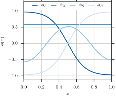
The only constant solution of this equation is the trivial fixed point $\phi(x)=0$, whose stability depends on $\alpha$ and $\kappa$. In the following, we choose $\alpha=10^{-2}$ and $\kappa=2\cdot 10^{-2}$, and therefore are in the regime where $\phi(x)=0$ is unstable. Two stable fixed points obtained by solving (25) for these values of $\alpha$ and $\kappa$ are depicted in Fig. 8 (left) as $\phi_{A}$ and $\phi_{B}$, with $\phi_{A}=-\phi_{B}$.

The slow manifold $\mathcal{M}$ for this model is made of the solutions of

$$P(\kappa\phi_{xx}+\phi-\phi^{3})=0\,.$$ (26)

On this manifold the motion is driven solely via the slow term, $-\alpha\phi$, on a time scale of order $O(\alpha)$, and the noise. Equation (26) can be written as

$$\kappa\phi_{xx}+\phi-\phi^{3}=\lambda$$ (27)

where $\lambda$ is a parameter. As a result the slow manifold can be described as one-parameter families of solutions parametrized by $\lambda\in\mathbb{R}$ – in general there is more than one family because the manifold can have different branches corresponding to solutions of (25) with a different number of domain walls.

Indeed, the two-dimensional pitchfork bifurcation SDE model (21) can be seen as a two-dimensional approximation of a discretized version of (23): The projection $Pv=v-\int_{0}^{1}v\,dx$ reduces to $\frac{1}{2}Q$ for a discretization with $N_{x}=2$ grid points. The projection $Pv=-\partial_{x}^{2}v$ for periodic boundary conditions reduces to $2Q$ for the standard finite difference 3-point Laplace stencil for $N_{x}=2$. In that sense, the two-dimensional model (21) is a discrete approximation of (23) for either choice of $P$ with only $N_{x}=2$ degrees of freedom (when furthermore dropping the dissipation term, $\kappa=0$).

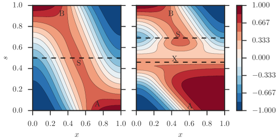
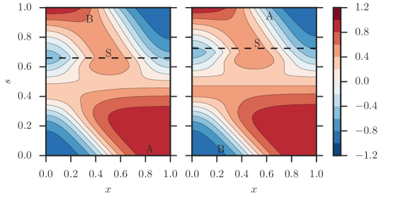
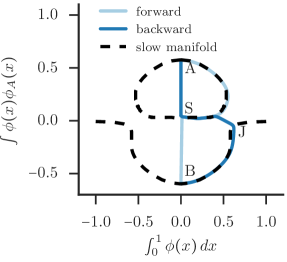
Fig. 7 (left) shows the heteroclinic orbit connecting the two stable fixed points: Along the complete trajectory, the mean is preserved. The transition follows a domain wall motion in the center, with a nucleation event at the boundary. The saddle point $\phi_{s}$, denoted by $S$, which also demarcates the position at which the separatrix is crossed, is the spatially symmetric configuration with a central region at $\phi=\phi_{+}$ and two regions at the boundary approaching $\phi=\phi_{-}$. In contrast, Fig. 7 (center) shows the minimizer of the action functional (6), representing the most probable transition path for $\epsilon\to 0$. Starting again at the fixed point $A$ this minimizer takes a different course, moving the domain wall, at vanishing cost for $\alpha\to 0$, without inducing nucleation. At the point $X$, close to the bifurcation point, the motion changes, tracking closely the separatrix (which is identical to the unstable portion of the slow manifold) into the saddle $S$. Note that the motion $X\to S$ happens quasi-deterministically despite introducing two nuclei at the boundaries, because of the slow drift pulling the mean towards $0$, while the projected term is $0$ exactly. From the saddle onward, $S\to B$, the transition necessarily follows the heteroclinic orbit, which is equivalent to the deterministic relaxation path. In this respect, the SPDE model (23) exactly corresponds to the two-dimensional model (21).

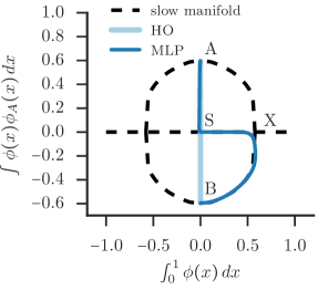
To further illustrate the resemblance to the two-dimensional model, we choose to project the minimizer, the heteroclinic orbit and the slow manifold onto two coordinates,

1. the mean $\int_{0}^{1}\phi(x)\,dx$, which corresponds to the direction $\phi_{1}+\phi_{2}$ of the two-dimensional model, and

2. the component of $\phi(x)$ in the direction of $\phi_{A}$ given by $\int_{0}^{1}\phi(x)\phi_{A}(x)\,dx$, which corresponds to the direction $\phi_{1}-\phi_{2}$ of the two-dimensional model.

The comparison of the transitions in the reduced coordinates is depicted in Fig. 7 (right). This figure is not a schematic, but the actual projection of the heteroclinic orbit and the minimizer of Fig. 7 (left, center) according to (i) and (ii) above. In this projected view, the separatrix is the straight vertical line, and the pitchfork bifurcation structure of the slow manifold is clearly visible, $X$ denoting the bifurcation point. The movement of the minimizer (dark blue) along the slow manifold (dashed) $A\to X$ and along the separatrix $X\to S$ (which coincides with the unstable part of the slow manifold) into the saddle $S$ highlights its difference to the relaxation pathway (light blue). The configurations at the points $A,B,S$ and $X$ are depicted in Fig. 8 (left).

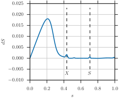
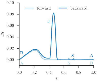
To demonstrate that the motion along the minimizer becomes quasi-deterministic already at $X$ before it hits the saddle at $S$, Fig. 8 (right) shows the action density $dS$ along the transition path. This quantity becomes nearly zero already at $X$.

5.2 Tilted Allen-Cahn/Cahn-Hilliard model

Figure 9: Forward (left) and backward (center) transitions in the tilted PDE model, $\phi_{\star}=3\cdot 10^{-2}\cos(x)$. Right: Projection of the forward and backward reactions into the bifurcation diagram. Note that the slow manifold becomes separated under the tilt and the forward transition becomes exponentially more likely than the backward transition.

Figure 10: Action density along forward and backward reaction. The jump at “J” between the slow manifolds leads to an $\mathcal{O}(\alpha)$ smaller action for the forward transition.

Similar to the two-dimensional reduction, the SPDE model (23) can also be tilted. Consequently, we are taking

$$\phi_{t}=P(\kappa\phi_{xx}+\phi-\phi^{3})-\alpha(\phi-\phi_{\star})+\sqrt{\epsilon}\,\eta(x,t),\qquad x\in[0,1]\,.$$ (28)

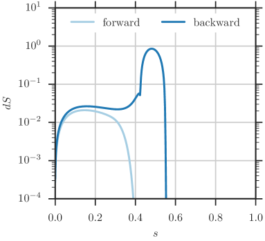
Again, a spatially homogeneous tilt $\phi_{\star}=\textrm{const.}$ will not result in a change in relative stability of the fixed points since the transitions and fixed points are still symmetric under $x\leftrightarrow 1-x$. If instead we tilt in a spatially inhomogeneous manner, we reproduce the segregation of the slow manifolds into two disconnected components, and the relative stability of the fixed points will change. The forward and backward transitions for the tilt $\phi_{\star}=3\cdot 10^{-2}\cos(\pi x)$ is depicted in Fig. 9 as well as its projection into the bifurcation diagram depicting the slow manifold of the system. The forward transition, starting from $A$, completely follows the slow manifold into the saddle $S$, to then move into the other fixed point $B$. In the opposite direction, before hitting the separatrix, the trajectory has to jump from one branch of the slow manifold to another at $J$. This jump is visible as a peak in the action density in Fig. 10. Note that the total action for forward and backward transition are drastically different, resulting again in an exponential difference in the relative stability of the two metastable fixed points. This is despite the fact that the spatial variation of the tilt is very small.

The interpretation in the context of motile bacteria and MIPS is the following: The spatially varying tilt $\phi_{\star}$ corresponds to a small spatial perturbation in the carrying capacity, i.e. to small spatial inhomogeneities in the availability of resources to sustain bacteria. Even tiny spatial variances lead to a separation of the slow manifold into multiple disconnected components. Whenever such a disconnected component does not contain a bifurcation point, or equivalently does not touch the separatrix, it will be easy to find by the noisy exploration of the dynamics, but hard to leave again. This translates into an exponentially amplified capability of motile bacteria to locally cluster around slightly increased food sources.

6 Conclusions

From a conceptual viewpoint at least, noise-induced transitions are relatively easy to analyze in systems whose dynamics satisfy detailed-balance (microscopic irreversibility). Indeed, large deviation theory indicates that, when the noise amplitude is small compared to the height of the barriers of the potential over which these systems navigate, the transitions proceed with high probability via reaction channels made out of heteroclinic orbits that connect local minima of the potential via saddle points. The situation is much more complex in systems whose dynamics are not in detailed-balance. In this set-up, there is no underlying potential, and the noise-induced transitions are intrinsically out-of-equilibrium phenomena. While large deviation theory still indicates that these transitions proceed by preferred channels (namely, the minimizer of the Freidlin-Wentzell action functional), these channels are not heteroclinic orbits in general, and their identification is nontrivial because of the wide variety of pathways they may take. While a general theory of such transitions remains elusive, here we have shown that some of their generic features can be identified in specific situations: namely slow-fast systems whose slow manifold displays bifurcations. In these systems, the slow manifold creates a preferred channel of reaction between the metastable states that typically differs vastly from the equilibrium prediction given by the heteroclinic orbit. The minimizer of the Freidlin-Wentzell action uses this channel, leading to an action that is lower by a factor $\alpha^{-1}$ compared to the one calculated along the heteroclinic orbit. Depending on the structure of the noise, this channel may or may not be used all the way through, but its existence allows one to develop robust numerical tools for the calculation of the actual minimizer of the Freidlin-Wentzell action. Such tools were proposed here. Interestingly, they apply not only in the limit of infinite time scale-separation, $\alpha\to 0$, but they can also be used in situations where a small but finite $\alpha$ may create order one discrepancies in the slow manifold structure that affect both the path of transition and the action along it. We expect these numerical tools to be therefore applicable in a wide range of situations with strong but not infinite time scale separation between slow and fast variables.

Appendix A Numerical computation of the transition trajectory

Consider the SDE

$$dZ=b(Z)\,dt+\sqrt{\epsilon}\sigma(Z)\,dW\,,$$ (29)

for $Z\in\mathbb{R}^{n}$, which includes the slow-fast dynamics (4) as a special case. Here, $W$ is a Wiener process on $\mathbb{R}^{n}$, $b:\mathbb{R}^{n}\to\mathbb{R}^{n}$ describes the deterministic dynamics and $\sigma:\mathbb{R}^{n}\to\mathbb{R}^{n}\times\mathbb{R}^{n}$ denotes the noise correlation. Large deviation theory specifies that the probability for the process $Z$ to end up in a set $B\subset\mathbb{R}^{n}$ is given by

$$\mathbb{P}^{z_{0}}(Z(T)\in B)\asymp\exp\big{(}-\epsilon^{-1}\min_{z\in\mathcal{C}}S_{T}(z)\big{)}\,,$$ (30)

where $\asymp$ denotes log-asymptotic equivalence and the minimum is taken over the set of functions $\mathcal{C}=\{z\in C([0,T],\mathbb{R}^{n}):z(0)=z_{0},z(T)\in B\}$. The action functional $S_{T}(z)$ is given by

$$S_{T}(z)=\int_{0}^{T}L(z,\dot{z})\,dt$$ (31)

for the Lagrangian

$$L(z,\dot{z})=\tfrac{1}{2}|\sigma^{-1}(\dot{z}-b(z))|^{2}\,.$$ (32)

LDT furthermore predicts the most likely transition pathway (MLP), or more precisely

$$\lim_{\epsilon\to 0}\mathbb{P}^{x}(\sup_{t\in[0,T]}|Z(t)-z_{\star}(t)|<\delta\ |\ Z(T)\in B)=1,\quad\forall\,\delta>0\,.$$ (33)

The MLP is given by the minimizer of the action functional,

$$z_{\star}=\mathop{\text{argmin }}_{z\in\mathcal{C}}S_{T}(z)\,.$$ (34)

From a numerical viewpoint, finding the transition probability (30) and the most likely transition $z_{\star}$ itself reduces to the deterministic optimization problem given by (34). Since the search space is a function space, this optimization problem can become quite large, in particular if the underlying system is spatially continuous (the SPDE case). In principle, though, it can be solved by numerical optimization techniques.

The optimization problem (34) becomes particularly intricate if we furthermore do not want to prescribe a transition time $T$, but instead are interested for example in the relative probability of the system to be found close to a given metastable fixed point or the mean first passage time between different metastable fixed points. These quantities are precisely defined in the context of LDT through the quasipotential

$$V(z_{A},z_{B})=\inf_{T>0}\min_{z\in\mathcal{C}_{z_{A},z_{B}}}S_{T}(z)\,,$$ (35)

where $\mathcal{C}_{z_{A},z_{B}}=\{z\in C([0,T],\mathbb{R}^{n}):z(0)=z_{A},z(T)=z_{B}\}$. Then, the mean first passage time $\tau_{A\to B}=\inf\{t>0:Z(t)\in B_{\delta}(z_{B}),Z(0)=z_{A}\}$ between $z_{A}$ and a ball of radius $\delta\ll 1$ around $z_{B}$ is given by

$$\mathbb{E}\tau_{A\to B}\asymp\exp(\epsilon^{-1}V(z_{A},z_{B}))\,,$$ (36)

and the relative probability to find the system close to $z_{A}$ and $z_{B}$ by

$$\frac{p_{A}}{p_{B}}\asymp\exp(\epsilon^{-1}(V(z_{A},z_{B})-V(z_{B},z_{A}))\,.$$ (37)

Unfortunately, in general, the minimization over $T$ in the computation of the quasipotential (35) will not be attained, i.e. $T\to\infty$. Numerically, this implies that we need to discretize an infinitely long time interval, which complicates the computation considerably.

An effective solution to this difficulty was proposed in [16, 17] by considering a geometric reformulation of the problem. Effectively, the computation of the quasipotential can also be expressed as

$$V(z_{A},z_{B})=\min_{z\in\mathcal{C}_{z_{A},z_{B}}}\sup_{\theta:H(z,\theta)=0}\int_{0}^{1}\langle\dot{z},\theta\rangle\,ds\,,$$ (38)

where $H(z,\theta)$ is the Hamiltonian corresponding to the Lagrangian (32) defined through

$$H(z,\theta)=\langle b(z),\theta\rangle+\tfrac{1}{2}|\sigma(z)\theta|^{2}\,,$$ (39)

and $\langle\cdot,\cdot\rangle$ denotes an appropriate inner product. In essence, the formulation (38) can be understood as Maupertius’ principle from classical mechanics: The integral in (38) no longer integrates over a (possibly infinite) time interval, but instead is independent of the parametrization of the trajectory $z$. As a consequence, the Euler-Lagrange equations are replaced by a least action principle over arc-length parametrized trajectories. The numerical difficulty of an optimization problem on infinite time horizons is reduced to a minimization problem on geodesics of finite length.

The numerical computation of the large deviation minimizers for all applications in this paper make use of this approach. For the associated optimization problem, we use the algorithm presented in [17], which generalizes those introduced in [35, 16].

Appendix B Numerical computation of the slow manifold

The slow manifold

$$\mathcal{M}=\{z\in\mathbb{R}^{d}|f(z)=0\}$$ (40)

can be defined solely on basis of the fast dynamics. In cases where the slow manifold is 1-dimensional (as is the case in all examples given above), we can identify all points on the slow manifold by sweeping through the possible values of the (scalar) control parameter $\mu$. Note that in this case the stable branches of the slow manifold $\mathcal{M}$ are readily found by relaxing the fast dynamics

$$\dot{z}=f(z)\,,$$ (41)

i.e. relaxing equation (41) for long times until convergence. The same is not true for the unstable branches, bifurcation points, etc, which cannot be obtained by this procedure.

Instead, we propose a scheme based on the string method [18, 19]. In simplified terms, the string method computes the heteroclinic orbit between stable fixed points by relaxing an elastic “string” between them. Applied to the problem at hand of computing $\mathcal{M}$ along $\mu$, choose a fixed value $\mu_{0}$ and compute two fixed points $z_{A}$ and $z_{B}$ of the fast dynamics (41) in the subspace $\mu=\mu_{c}$. Since the fast dynamics leave the control parameter $\mu$ invariant, it is sufficient to choose initial conditions which fulfill $\mu=\mu_{c}$. Of course, $z_{i},i=A,B$ is the intersection point of $\mathcal{M}$ with the subset $\mu=\mu_{c}$, and consequently $z_{i}\in\mathcal{M}$. Now, consider a family of configurations $\bar{z}(t,s)\in\mathbb{R}^{d}$, with $s\in[0,1]$ (the “string”), with $\bar{z}(t,0)=z_{A}$ and $\bar{z}(t,1)=z_{B}$, in this subspace, connecting the two fixed points. Relax this family of configurations according to

$$\partial_{t}\bar{z}(t,s)=(1-\hat{t}\otimes\hat{t})f(\bar{z}(t,s))\qquad\forall\,s\,\in\,[0,1]\,,$$

where $\hat{t}=\partial_{s}\bar{z}(t,s)/|\partial_{s}\bar{z}(t,s)|$ is the unit tangent vector along the string and therefore $(1-\hat{t}\otimes\hat{t})$ projects onto the component normal to the string. After convergence, the resulting string will necessarily have that $\partial_{s}\bar{z}(t,s)$ is parallel to $f(z(t,s))$ everywhere, and thus forms the heteroclinic orbit between $z_{A}$ and $z_{B}$. Since this heteroclinic orbit necessarily contains a saddle point $z_{S}$, which is easily found by identifying the value of $s$ for which $f(z(t,s))=0$, we have identified the unstable branch of $\mathcal{M}$ in the subspace $\mu=\mu_{c}$. Repeating the procedure for all values of $\mu_{c}$, we can line out the complete slow manifold. Bifurcation points are identified by points where stable fixed points merge with saddles. In the case of the subcritical pitchfork bifurcation, we can even identify all 5 branches of $\mathcal{M}$ in a single string. The slow manifolds of all infinite dimensional applications above have been computed by this method. In the finite dimensional case, the slow manifold is often available analytically.

References

- [1] Berglund N and Gentz B 2006 Noise-Induced Phenomena in Slow-Fast Dynamical Systems: A Sample-Paths Approach (Springer Science & Business Media) ISBN 978-1-84628-186-0
- [2] Kuehn C 2011 Physica D: Nonlinear Phenomena 240 1020 – 1035
- [3] Freidlin M I and Wentzell A D 1998 Random perturbations of dynamical systems (Springer)
- [4] Berglund N and Gentz B 2002 Stochastics and Dynamics 02 327–356
- [5] Pikovsky A S and Kurths J 1997 Physical Review Letters 78 775–778 ISSN 0031-9007, 1079-7114
- [6] Freidlin M I 2001 Journal of Statistical Physics 103 283–300
- [7] Freidlin M I 2001 Stochastics and Dynamics 01 261–281
- [8] Muratov C B, Vanden-Eijnden E and Weinan E 2005 Physica D: Nonlinear Phenomena 210 227–240
- [9] DeVille R E L, Vanden-Eijnden E and Muratov C B 2005 Physical Review E 72 031105
- [10] Freidlin M I 1978 Russian Mathematical Surveys 33 117–176
- [11] Kifer Y 1992 Inventiones mathematicae 110 337–370 ISSN 0020-9910, 1432-1297
- [12] Veretennikov A Y 2000 Stochastic Processes and their Applications 89 69–79 ISSN 0304-4149
- [13] Bouchet F, Grafke T, Tangarife T and Vanden-Eijnden E 2016 Journal of Statistical Physics 162 793–812
- [14] Maier R and Stein D 1997 SIAM Journal on Applied Mathematics 57 752–790 ISSN 0036-1399
- [15] Bouchet F and Touchette H 2012 Journal of Statistical Mechanics: Theory and Experiment 2012 P05028 ISSN 1742-5468
- [16] Heymann M and Vanden-Eijnden E 2008 Communications on Pure and Applied Mathematics 61 1052–1117 ISSN 1097-0312
- [17] Grafke T, Schäfer T and Vanden-Eijnden E 2016 arXiv:1604.03818 [cond-mat]
- [18] E W, Ren W and Vanden-Eijnden E 2002 Physical Review B 66 052301
- [19] E W, Ren W and Vanden-Eijnden E 2007 J. Chem. Phys. 126 164103
- [20] FitzHugh R 1961 Biophysical Journal 1 445–466 ISSN 0006-3495
- [21] Nagumo J, Arimoto S and Yoshizawa S 1962 Proceedings of the IRE 50 2061–2070 ISSN 0096-8390
- [22] Hodgkin A L and Huxley A F 1952 The Journal of Physiology 117 500–544 ISSN 0022-3751
- [23] Ludwig D, Jones D D and Holling C S 1978 Journal of Animal Ecology 47 315–332 ISSN 0021-8790
- [24] Strogatz S H 2014 Nonlinear Dynamics and Chaos: With Applications to Physics, Biology, Chemistry, and Engineering (Westview Press) ISBN 978-0-8133-4910-7
- [25] Hairer M 2014 Inventiones mathematicae 198 269–504 ISSN 0020-9910, 1432-1297
- [26] Faris W G and Jona-Lasinio G 1982 J. of Phys. A 15 3025
- [27] Bertini L, De Sole A, Gabrielli D, Jona-Lasinio G and Landim C 2015 Reviews of Modern Physics 87 593–636
- [28] Allen S and Cahn J 1972 Acta Metallurgica 20 423–433 ISSN 00016160
- [29] Cahn J W and Hilliard J E 1958 The Journal of Chemical Physics 28 258–267 ISSN 0021-9606, 1089-7690
- [30] Wittkowski R, Tiribocchi A, Stenhammar J, Allen R J, Marenduzzo D and Cates M E 2014 Nature Communications 5 4351
- [31] Tailleur J and Cates M E 2008 Physical Review Letters 100 218103
- [32] Cates M E and Tailleur J 2015 Annual Review of Condensed Matter Physics 6 219–244
- [33] Cates M E, Marenduzzo D, Pagonabarraga I and Tailleur J 2010 Proceedings of the National Academy of Sciences 107 11715–11720 ISSN 0027-8424, 1091-6490
- [34] Grafke T, Cates M E and Vanden-Eijnden E 2017 arXiv:1703.06923 [cond-mat] ArXiv: 1703.06923
- [35] E W, Ren W and Vanden-Eijnden E 2004 Comm. Pure Appl. Math. 57 637–656