Rattleback dynamics and its reversal time of rotation

Abstract

A rattleback is a rigid, semi-elliptic toy which exhibits unintuitive behavior; when it is spun in one direction, it soon begins pitching and stops spinning, then it starts to spin in the opposite direction, but in the other direction, it seems to spin just steadily. This puzzling behavior results from the slight misalignment between the principal axes for the inertia and those for the curvature; the misalignment couples the spinning with the pitching and the rolling oscillations. It has been shown that under the no-slip condition and without dissipation the spin can reverse in both directions, and Garcia and Hubbard obtained the formula for the time required for the spin reversal $t_{r}$ [Proc. R. Soc. Lond. A 418, 165 (1988)]. In this work, we reformulate the rattleback dynamics in a physically transparent way and reduce it to a three-variable dynamics for spinning, pitching, and rolling. We obtain an expression of the Garcia-Hubbard formula for $t_{r}$ by a simple product of four factors: (1) the misalignment angle, (2) the difference in the inverses of inertia moment for the two oscillations, (3) that in the radii for the two principal curvatures, and (4) the squared frequency of the oscillation. We perform extensive numerical simulations to examine validity and limitation of the formula, and find that (1) the Garcia-Hubbard formula is good for both spinning directions in the small spin and small oscillation regime, but (2) in the fast spin regime especially for the steady direction, the rattleback may not reverse and shows a rich variety of dynamics including steady spinning, spin wobbling, and chaotic behavior reminiscent of chaos in a dissipative system.

I Introduction

Spinning motions of rigid bodies have been studied for centuries and still are drawing interest in recent years, including the motions of Euler’s disks Moffatt (2000), spinning eggs Moffatt and Shimomura (2002), and rolling rings Jalali et al. (2015), to mention just a few. Also, macroscopic systems which convert vibrations to rotations have been studied in various context such as a circular granular ratchet Heckel et al. (2012), and bouncing dumbbells, which show a cascade of bifurcations Kubo et al. (2015). Another interesting example of rigid body dynamics which involves such oscillation-rotation coupling is a rattleback, also called as a celt or wobble stone, which is a semi-elliptic spinning toy [Fig. 1(a)]. It spins smoothly when spun in one direction; however, when spun in the other direction, it soon starts wobbling or rattling about its short axis and stops spinning, then it starts to rotate in the opposite direction. One who has studied classical mechanics must be amazed by this reversal in spinning, because it apparently seems to violate the angular momentum conservation, and the chirality emerges from a seemingly symmetrical object.

There are three requirements for a rattleback to show this reversal of rotation: (1) the two principal curvatures of the lower surface should be different, (2) the two horizontal principal moments of inertia should also be different, and (3) the principal axes of inertia should be misaligned to the principal directions of curvature. These characteristics induce the coupling between the spinning motion and the two oscillations: the pitching about the short horizontal axis and the rolling about the long horizontal axis. The coupling is asymmetric, i.e., the oscillations cause torque around the spin axis and the signs of the torque are opposite to each other. This also means that either the pitching or the rolling is excited depending on the direction of the spinning. We will see that the spinning couples with the pitching much stronger than that with the rolling; therefore, it takes much longer time for spin reversal in one direction than in the other direction, and that is why most rattlebacks reverse only for one way before they stop by dissipation.

In the 1890s, a meteorologist, Walker, performed the first quantitative analysis of the rattleback motion Walker (1896). Under the assumptions that the rattleback does not slip at the contact point and that the rate of spinning speed changes much slower than other time scales, he linearized the equations of motion and showed that either the pitching or the rolling becomes unstable depending on the direction of the spin. More detailed analyses were performed by Bondi Bondi (1986), and recently by Wakasugi Wakasugi (2011). Case and Jalal Case and Jalal (2014) derived the growth rate of instability at slow spinning. Markeev Markeev (1983), Pascal Pascal (1983), and Blackowiak et al. Blackowiak et al. (1997) obtained the equations of the spin motion by extracting the slowly varying amplitudes of the fast oscillations of the pitching and the rolling. Moffatt and Tokieda Moffatt and Tokieda (2008) derived similar equations to those of Markeev Markeev (1983) and Pascal Pascal (1983), and pointed out the analogy to the dynamo theory. Garcia and Hubbard Garcia and Hubbard (1988) obtained the expressions of the averaged torques generated by the pure pitching and the rolling, and derived the formula for spin reversal time.

As the first numerical study, Kane and Levinson Kane and Levinson (1982) simulated the energy-conserving equations and showed that the rattleback changes its spinning direction indefinitely for certain parameter values and initial conditions. They also demonstrated the coupling between the oscillations and the spinning by showing that it starts to rotate when it begins with pure pitching or rolling, but the direction of the rotation is different between pitching and rolling. Similar simulations were performed by Lindberg and Longman independently Lindberg and Longman (1983). Nanda et al. simulated the spin resonance of the rattleback on a vibrating base Nanda et al. (2016).

Energy-conserving dynamical systems usually conserve the phase volume, but the present rattleback dynamics does not explore the whole phase volume with a given energy because of a non-holonomic constraint due to the no-slip condition. Therefore, the Liouville theorem does not hold, and such a system has been shown to behave much like dissipative systems. Borisov and Mamaev in fact reported the existence of “strange attractor” for certain parameter values in the present system Borisov and Mamaev (2003). The no-slip rattleback system has been actively studied in the context of chaotic dynamics during the last decade Borisov et al. (2006, 2014).

Effects of dissipation at the contact point have been investigated in several works. Magnus Magnus (1974) and Karapetyan Karapetyan (1981) incorporated a viscous type of friction force proportional to the velocity. Takano Takano (2014) determined the conditions under which the reversal of rotation occurs with the viscous dissipation. Garcia and Hubbard Garcia and Hubbard (1988) simulated equations with aerodynamic force, Coulomb friction in the spinning, and dissipation due to slippage, then they compared the results with a real rattleback. The dissipative rattleback models based on the contact mechanics with Coulomb friction have been developed by Zhuravlev and Klimov Zhuravlev and Klimov (2008) and Kudra and Awrejcewicz Awrejcewicz and Kudra (2012); Kudra and Awrejcewicz (2013, 2015).

This paper is organized as follows. In the next section, we reformulate the rattleback dynamics under the no-slip and no dissipation condition in a physically transparent way. In the small-spin and small-oscillation approximation, the dynamics is reduced to a simplified three-variable dynamics. We then focus on the time required for reversal, or what we call the time for reversal, which is the most evident quantity that characterizes rattlebacks, and obtain a concise expression for the Garcia-Hubbard formula for the time for reversal Garcia and Hubbard (1988). In Sec. III, the results of the extensive numerical simulations are presented for various model parameters and initial conditions in order to examine the validity and the limitation of the theory. Discussions and conclusion are given in Sec. IV and Sec. V, respectively.

II Theory

II.1 Equations of motion

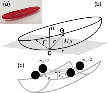
Figure 1: (a) A commercially available rattleback made of plastic. (b) Notations of the rattleback. (c) A schematic illustration of the shell-dumbbell model.

We consider a rattleback as a rigid body, whose configuration can be represented by the position of the center of mass G and the Euler angles; both of them are obtained by integrating the velocity of the center of mass $\bm{v}$ and the angular velocity $\bm{\omega}$ around it Goldstein et al. (2002).

We investigate the rattleback motion on a horizontal plane, assuming that it is always in contact with the plane at a single point C without slipping. We ignore dissipation, then all the forces that act on the rattleback are the contact force $\bm{F}$ exerted by the plane at C and the gravitational force $-Mg\bm{u}$, where $\bm{u}$ represents the unit vertical vector pointing upward [Fig. 1(b)]. Therefore, the equations of motion are given by

$$\frac{d(M\bm{v})}{dt} =\bm{F}-Mg\bm{u},$$ (1)

$$\frac{d(\hat{I}\bm{\omega})}{dt} =\bm{r}\times\bm{F},$$ (2)

where $M$ and $\hat{I}$ are the mass and the inertia tensor around G, respectively, and $\bm{r}$ is the vector from G to the contact point C.

The contact force $\bm{F}$ is determined by the conditions of the contact point; our assumptions are that (1) the rattleback is always in contact at a point with the plane, and (2) there is no slip at the contact point. The second constraint is represented by the relation

$$\bm{v}=\bm{r}\times\bm{\omega}.$$ (3)

Before formulating the constraint (1), we specify the co-ordinate system. We employ the body-fixed co-ordinate with the origin being the center of mass G, and the axes being the principal axes of inertia; the $z$ axis is the one close to the spinning axis pointing downward, and the $x$ and $y$ axes are taken to be $I_{xx}>I_{yy}$ (Fig. 2).

In this co-ordinate, the lower surface function of the rattleback is assumed to be given by

$$f(x,y,z)=0,$$ (4)

where

$$f(x,y,z)\equiv\frac{z}{a}-1+\frac{1}{2a^{2}}(x,\,y)\hat{R}(\xi)\hat{\Theta}\hat{R}^{-1}(\xi)\begin{pmatrix}x\\ y\\ \end{pmatrix},$$ (5)

with

$$\hat{R}(\xi)\equiv\begin{pmatrix}\cos\xi,&-\sin\xi\\ \sin\xi,&\cos\xi\\ \end{pmatrix},\quad\hat{\Theta}\equiv\begin{pmatrix}\theta,&0\\ 0&\phi\\ \end{pmatrix}.$$ (6)

Here $a$ is the distance between G and the surface at $x=y=0$, and $\xi$ is the skew angle by which the principal directions of curvature are rotated from the $x$-$y$ axes, which we choose as the principal axes of inertia (Fig. 2). $\theta/a$ and $\phi/a$ are the principal curvatures at the bottom, namely at $(0,0,a)^{t}$.

Now, we can formulate the contact point condition (1); the components of the contact point vector $\bm{r}$ should satisfy Eq. (4), and the normal vector of the surface at C should be parallel to the vertical vector $\bm{u}$. Thus we have

$$\bm{u}\parallel\nabla f,$$ (7)

which gives the relation

$$\frac{\bm{r}_{\perp}}{a}=\frac{1}{u_{z}}\hat{R}(\xi)\hat{\Theta}^{-1}\hat{R}^{-1}(\xi)\bm{u}_{\perp},$$ (8)

where $\bm{a}_{\perp}$ represents the $x$ and $y$ components of a vector $\bm{a}$ in the body-fixed co-ordinate.

Before we proceed, we introduce a dotted derivative of a vector $\bm{a}$ defined as the time derivative of the vector components in the body-fixed co-ordinate. This is related to the time derivative by

$$\frac{d\bm{a}}{dt}=\dot{\bm{a}}+\bm{\omega}\times\bm{a}.$$ (9)

Note that the vertical vector $\bm{u}$ does not depend on time, thus we have

$$\frac{d\bm{u}}{dt}=\dot{\bm{u}}+\bm{\omega}\times\bm{u}=\bm{0}.$$ (10)

These conditions, i.e., the no-slip condition (3), the conditions of the contact point (4) and (8), and the vertical vector condition (10), close the equations of motion (1) and (2).

Following Garcia and Hubbard Garcia and Hubbard (1988), we describe the rattleback dynamics by $\bm{u}$ and $\bm{\omega}$. The evolution of $\bm{\omega}$ is obtained as

$$\hat{I}\dot{\bm{\omega}}-M\bm{r}\times(\bm{r}\times\dot{\bm{\omega}})=-\bm{\omega}\times(\hat{I}\bm{\omega})\\ +M\bm{r}\times(\dot{\bm{r}}\times\bm{\omega}+\bm{\omega}\times(\bm{r}\times\bm{\omega}))+Mg\bm{r}\times\bm{u}$$ (11)

by eliminating the contact force $\bm{F}$ from the equations of motion (1) and (2), and using the no-slip condition (3). The state variables $\bm{u}$ and $\bm{\omega}$ can be determined by Eqs. (10) and (11) with the contact point conditions (4) and (8).

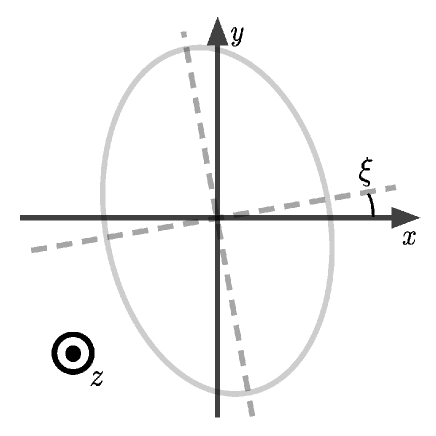
Figure 2: (color online) A body-fixed co-ordinate viewed from below. The dashed lines indicate the principal directions of curvature, rotated by $\xi$ from the principal axes of inertia (the $x$-$y$ axes).

The rattleback is characterized by the inertial parameters $M$, $I_{xx}$, $I_{yy}$, $I_{zz}$, the geometrical parameters $\theta$, $\phi$, $a$, and the skew angle $\xi$. For the stability of the rattleback, both of the dimensionless curvatures $\theta$ and $\phi$ should be smaller than $1$; without loss of generality, we assume

$$0<\phi<\theta<1,$$ (12)

then, it is enough to consider

$$-\frac{\pi}{2}<\xi<0,$$ (13)

for the range of the skew angle $\xi$. The positive $\xi$ case can be obtained by the reflection with respect to the $x$-$z$ plane.

At this stage, we introduce the dimensionless inertial parameters $\alpha$, $\beta$, and $\gamma$ for later use after Bondi Bondi (1986) as

$$\alpha\equiv\frac{I_{xx}}{Ma^{2}}+1,\ \beta\equiv\frac{I_{yy}}{Ma^{2}}+1,\ \gamma\equiv\frac{I_{zz}}{Ma^{2}},$$ (14)

which are dimensionless inertial moments around the contact point C. Note that

$$\alpha>\beta>1,$$ (15)

because we have assumed $I_{xx}>I_{yy}$.

II.2 Small amplitude approximation of oscillations under $\omega_{z}=0$

We consider the oscillation modes in the case of no spinning $\omega_{z}=0$ in the small amplitude approximation, namely, in the linear approximation in $|\omega_{x}|,\,|\omega_{y}|\ll\sqrt{g/a}$, which leads to $|x|,\,|y|\ll a$, $|u_{x}|,\,|u_{y}|\ll 1$, and $u_{z}\approx-1$. In this regime, the $x$ and $y$ components of Eq. (10) can be linearized as

$$\dot{\bm{u}}_{\perp}\approx\hat{\varepsilon}\,\bm{\omega}_{\perp},\quad\hat{\varepsilon}\equiv\begin{pmatrix}0,&1\\ -1,&0\\ \end{pmatrix}=\hat{R}(-\pi/2).$$ (16)

By using Eq. (8) with $u_{z}\approx-1$, Eq. (11) can be linearized as

$$\hat{J}\,\dot{\bm{\omega}}_{\perp} \approx\frac{g}{a^{2}}(\bm{r}\times\bm{u})_{\perp}$$

$$=-\frac{g}{a}\hat{\varepsilon}\,[-\hat{R}(\xi)\hat{\Theta}^{-1}\hat{R}^{-1}(\xi)+1]\bm{u}_{\perp},$$ (17)

with the inertial matrix

$$\hat{J}\equiv\begin{pmatrix}\alpha,&0\\ 0,&\beta\\ \end{pmatrix}.$$ (18)

From the linearized equations (16) and (17), we obtain

$$\hat{J}\ddot{\bm{\omega}}_{\perp}=-\frac{g}{a}(\hat{\Gamma}-1)\bm{\omega}_{\perp},$$ (19)

where

$$\hat{\Gamma}\equiv\hat{R}(\xi+\pi/2)\hat{\Theta}^{-1}\hat{R}^{-1}(\xi+\pi/2).$$ (20)

At this point, it is convenient to introduce the bra-ket notation for the row and column vector of $\bm{\omega}_{\perp}$ as $\bra{\omega_{\perp}}$ and $\ket{\omega_{\perp}}$, respectively. With this notation, Eq. (19) can be put in the form of

$$\ket{\ddot{\tilde{\omega}}_{\perp}}=-\hat{H}\ket{\tilde{\omega}_{\perp}},$$ (21)

with

$$\ket{\tilde{\omega}_{\perp}}\equiv\hat{J}^{1/2}\ket{\omega_{\perp}},\quad\hat{H}\equiv\frac{g}{a}\hat{J}^{-1/2}(\hat{\Gamma}-1)\hat{J}^{-1/2},$$ (22)

where $\hat{H}$ is symmetric. The eigenvalue equation

$$\hat{H}\ket{\tilde{\omega}_{j}}=\omega_{j}^{2}\ket{\tilde{\omega}_{j}}$$ (23)

determines the two oscillation modes with $j=p$ or $r$, whose frequencies are given by

$$\omega_{p,r}^{2}=\frac{1}{2}\left[(H_{11}+H_{22})\pm\sqrt{(H_{11}-H_{22})^{2}+4H_{12}^{2}}\right]$$ (24)

with

$$\omega_{p}\geq\omega_{r}.$$ (25)

Here, $H_{ij}$ denotes the $ij$ component of $\hat{H}$. The orthogonal condition for the eigenvectors $\ket{\tilde{\omega}_{p}}$ and $\ket{\tilde{\omega}_{r}}$ can be written using $\hat{\varepsilon}$ as

$$\ket{\tilde{\omega}_{p}} =\hat{\varepsilon}\ket{\tilde{\omega}_{r}},\quad\ket{\tilde{\omega}_{r}}=-\hat{\varepsilon}\ket{\tilde{\omega}_{p}},$$ (26)

$$\bra{\tilde{\omega}_{r}} =\bra{\tilde{\omega}_{p}}\hat{\varepsilon},\quad\bra{\tilde{\omega}_{p}}=-\bra{\tilde{\omega}_{r}}\hat{\varepsilon}.$$ (27)

In the case of zero skew angle, $\xi=0$, we have

$$\omega_{p}^{2} =\left({g\over a}\right){1/\phi-1\over\alpha}\equiv\omega_{p0}^{2},$$ (28)

$$\omega_{r}^{2} =\left({g\over a}\right){1/\theta-1\over\beta}\equiv\omega_{r0}^{2},$$ (29)

and the eigenvectors $\ket{\omega_{p}}$ and $\ket{\omega_{r}}$ are parallel to the $x$ and the $y$ axes, thus these modes correspond to the pitching and the rolling oscillations, respectively. This correspondence holds for $|\xi|\ll 1$ and $\omega_{p0}>\omega_{r0}$ as for a typical rattleback parameter, the case we will discuss mainly in the following .

II.3 Garcia and Hubbard’s theory for the time for reversal

Based on our formalism, it is quite straightforward to derive Garcia and Hubbard’s formula for the reversal time of rotation.

II.3.1 Asymmetric torque coefficients

Due to the skewness, the pitching and the rolling are coupled with the spinning motion. We examine this coupling in the case of $\omega_{z}=0$ by estimating the averaged torques around the vertical axis caused by the pitching and the rolling oscillations. From Eqs. (1) and (2) and the no-slip condition Eq. (3), the torque around $\bm{u}$ is given by

$$T \equiv\bm{u}\cdot(\bm{r}\times\bm{F})\approx-Ma^{2}[\dot{\bm{\omega}}_{\perp}\cdot\hat{\varepsilon}(\hat{\Gamma}-1)\hat{\varepsilon}\,\bm{u}_{\perp}\,],$$ (30)

within the linear approximation in $\bm{\omega}_{\perp}$, $\bm{u}_{\perp}$, and $\bm{r}_{\perp}$ discussed in Sec. II.2.

We define the asymmetric torque coefficients $K_{p}$ and $K_{r}$ for each mode by

$$-K_{p}\equiv\frac{\overline{T}_{p}}{\overline{E}_{p}},\qquad K_{r}\equiv\frac{\overline{T}_{r}}{\overline{E}_{r}},$$ (31)

where $\overline{T}_{j}\ (j=p\text{~{}or~{}}r)$ is the averaged torque over the oscillation period generated by each mode, and $\overline{E}_{j}$ is the corresponding averaged oscillation energy which can be estimated within the linear approximation as

$$\overline{E} \approx Ma^{2}(\alpha\overline{\omega_{x}^{2}}+\beta\overline{\omega_{y}^{2}}).$$ (32)

The minus sign for the definition of $K_{p}$ is inserted in order that both $K_{p}$ and $K_{r}$ should be positive for typical rattleback parameters as can be seen below. Note that the asymmetric torque coefficients are dimensionless.

From Eqs. (30) and (32), $-K_{p}$ is given by

$$-K_{p} =\frac{\braket{\omega_{p}}{\,\hat{\varepsilon}(\hat{\Gamma}-1)\hat{\varepsilon}\hat{\varepsilon}\,}{\omega_{p}}}{\braket{\omega_{p}}{\hat{J}}{\omega_{p}}}$$

$$=-\frac{(a/g)\braket{\tilde{\omega}_{p}}{\,\hat{J}^{-1/2}\hat{\varepsilon}\hat{J}^{1/2}\hat{H}\,}{\tilde{\omega}_{p}}}{\braket{\tilde{\omega}_{p}}{\tilde{\omega}_{p}}}$$ (33)

$$=-\omega_{p}^{2}\,\frac{(a/g)\braket{\tilde{\omega}_{p}}{\,\hat{J}^{-1/2}\hat{\varepsilon}\hat{J}^{1/2}\,}{\tilde{\omega}_{p}}}{\braket{\tilde{\omega}_{p}}{\tilde{\omega}_{p}}}.$$ (34)

In the same way, $K_{r}$ is given by

$$K_{r} =-\frac{(a/g)\braket{\tilde{\omega}_{r}}{\hat{J}^{-1/2}\hat{\varepsilon}\hat{J}^{1/2}\hat{H}}{\tilde{\omega}_{r}}}{\braket{\tilde{\omega}_{r}}{\tilde{\omega}_{r}}}$$ (35)

$$=\omega_{r}^{2}\,\frac{(a/g)\braket{\tilde{\omega}_{p}}{(\hat{J}^{-1/2}\hat{\varepsilon}\hat{J}^{1/2})^{\dagger}}{\tilde{\omega}_{p}}}{\braket{\tilde{\omega}_{p}}{\tilde{\omega}_{p}}}.$$ (36)

Equations (33)–(36) yield simple relations for $K_{p}$ and $K_{r}$ as

$$\frac{K_{p}}{K_{r}}=\frac{\omega_{p}^{2}}{\omega_{r}^{2}}$$ (37)

and

$$K_{p}-K_{r} =\frac{(a/g)}{\braket{\tilde{\omega}_{p}}{\tilde{\omega}_{p}}}\mathrm{Tr}\left[\hat{J}^{-1/2}\hat{\varepsilon}\hat{J}^{-1/2}\hat{H}\right]$$

$$=-\frac{1}{2}\sin(2\xi)\left(\frac{1}{\beta}-\frac{1}{\alpha}\right)\left(\frac{1}{\phi}-\frac{1}{\theta}\right).$$ (38)

Equations (37) and (38) are enough to determine

$$K_{p}=-\frac{1}{2}\sin(2\xi)\left(\frac{1}{\beta}-\frac{1}{\alpha}\right)\left(\frac{1}{\phi}-\frac{1}{\theta}\right)\frac{\omega_{p}^{2}}{\omega_{p}^{2}-\omega_{r}^{2}},$$ (39)

$$K_{r}=-\frac{1}{2}\sin(2\xi)\left(\frac{1}{\beta}-\frac{1}{\alpha}\right)\left(\frac{1}{\phi}-\frac{1}{\theta}\right)\frac{\omega_{r}^{2}}{\omega_{p}^{2}-\omega_{r}^{2}}.$$ (40)

Note that Eqs. (39) and (40) are consistent with the three requirements of rattlebacks: $\xi\neq 0$, $\alpha\neq\beta$, and $\theta\neq\phi$. Equations (39) and (40) are shown to be equivalent to the corresponding expressions Eq. (42a,b) in Garcia and Hubbard Garcia and Hubbard (1988) although their expressions look quite involved. These results also show that

$$K_{p}K_{r}>0\quad\text{and hence}\quad\overline{T}_{p}\overline{T}_{r}<0,$$ (41)

namely, the torques generated by the pitching and the rolling always have opposite signs to each other.

II.3.2 Typical rattleback parameters

Typical rattleback parameters fall in the region that satisfies the following two conditions: (1) the skew angle is small,

$$|\xi|\ll 1,$$ (42)

and (2) the pitch frequency is higher than the roll frequency. Under these conditions, the modes $p$ and $r$ of Eq. (23) correspond to the pitching and the rolling oscillations respectively, and

$$\omega_{p}^{2}\approx\omega_{p0}^{2},\qquad\omega_{r}^{2}\approx\omega_{r0}^{2}$$ (43)

in accord with the inequality (25) Note (1). From Eqs. (31), (39), and (40), the signs of the asymmetric torque coefficients and the averaged torques for typical rattlebacks are given by

$$K_{p}>0\quad\text{and}\quad K_{r}>0,$$ (44)

and

$$\overline{T}_{p}<0\quad\text{and}\quad\overline{T}_{r}>0,$$ (45)

by noting $\xi<0$, $\alpha>\beta$, $\theta>\phi$.

The fact that $\omega_{p0}>\omega_{r0}$ for a typical rattleback means that the shape factor, $1/\phi-1$ or $1/\theta-1$, contributes much more than the inertial factor, $1/\alpha$ or $1/\beta$, in Eqs. (28) and (29) although these two factors compete, i.e. $1/\phi-1>1/\theta-1$ and $1/\alpha<1/\beta$. This is a typical situation because the two curvatures of usual rattlebacks are markedly different, i.e., $\phi\ll\theta<1$ as can be seen in Fig. 1(c). Moreover, we can show that the pitch frequency is always higher for an ellipsoid with a uniform mass density whose surface is given by $x^{2}/c^{2}+y^{2}/b^{2}+z^{2}/a^{2}=1\ (b^{2}>c^{2}>a^{2})$. This also holds for a semi-ellipsoid for $b^{2}>c^{2}>(5/8)a^{2}$, where the co-ordinate system is the same as the ellipsoid.

II.3.3 Time for reversal

Now we study the time evolution of the spin $n$ defined as the vertical component of the angular velocity

$$n\equiv\bm{u}\cdot\bm{\omega},$$ (46)

assuming that the expressions for the asymmetric torque coefficients, $K_{p}$ and $K_{r}$, obtained above are valid even when $\omega_{z}\neq 0$. We consider the quantities $\overline{n}$, $\overline{E}_{p}$, and $\overline{E}_{r}$, averaged over the time scale much longer than the oscillation periods, yet much shorter than the time scale for spin change. Then, these averaged quantities should follow the following evolution equations:

$$I_{\textrm{eff}}\frac{d\overline{n}(t)}{dt} =-K_{p}\overline{E}_{p}(t)+K_{r}\overline{E}_{r}(t),$$ (47)

$$\frac{d\overline{E}_{p}(t)}{dt} =K_{p}\overline{n}(t)\overline{E}_{p}(t),$$ (48)

$$\frac{d\overline{E}_{r}(t)}{dt} =-K_{r}\overline{n}(t)\overline{E}_{r}(t).$$ (49)

Here, $I_{\textrm{eff}}$ is the effective moment of inertia around $\bm{u}$ under the existence of the oscillations, and is assumed to be constant; it should be close to $I_{zz}$. As can be seen easily, the total energy $E_{\textrm{tot}}$ defined by

$$E_{\textrm{tot}}\equiv\frac{1}{2}I_{\textrm{eff}}\overline{n}(t)^{2}+\overline{E}_{p}(t)+\overline{E}_{r}(t)$$ (50)

is conserved. It can be seen that there is another invariant,

$$C_{I}\equiv\frac{1}{K_{p}}\ln\overline{E}_{p}+\frac{1}{K_{r}}\ln\overline{E}_{r},$$ (51)

which has been discussed in connection with a Casimir invariant Moffatt and Tokieda (2008); Yoshida et al. (2016). With these two conservatives, general solutions of the three-variable system (47)–(49) should be periodic.

Let us consider the case where the spin is positive at $t=0$ and the sum of the oscillation energies are small compared to the spinning energy:

$$\overline{n}(0)\equiv n_{i}>0,\quad\overline{E}_{p}(0)+\overline{E}_{r}(0)\ll\frac{1}{2}I_{\textrm{eff}}n_{i}^{2}.$$ (52)

For a typical rattleback, the pitching develops and the rolling decays as long as $\overline{n}>0$ as can be seen from Eqs. (44), (48) and (49). Thus the rolling is irrelevant and can be ignored, i.e., $\overline{E}_{r}(t)=0$, to estimate the time for reversal. Then we can derive the equation

$$\frac{d\overline{n}(t)}{dt}=-\frac{K_{p}}{2}\left(n_{0}^{2}-\overline{n}(t)^{2}\right),$$ (53)

where the constant $n_{0}>0$ is defined by

$$\frac{1}{2}I_{\textrm{eff}}n_{0}^{2}\equiv E_{\textrm{tot}}.$$ (54)

This can be easily solved as

$$\overline{n}(t)=n_{0}\frac{(n_{0}+n_{i})\exp(-n_{0}K_{p}t)-(n_{0}-n_{i})}{(n_{0}+n_{i})\exp(-n_{0}K_{p}t)+(n_{0}-n_{i})},$$ (55)

and we obtain the time for reversal $t_{rGH+}$ for the $n_{i}>0$ case as

$$t_{rGH+}=\frac{1}{n_{0}K_{p}}\ln\left(\frac{n_{0}+n_{i}}{n_{0}-n_{i}}\right),$$ (56)

by just setting $\overline{n}=0$ in Eq. (55).

Similarly, in the case of $n_{i}<0$, only the rolling develops and the pitching is irrelevant, thus we obtain $\overline{n}(t)$ and the time for reversal $t_{rGH-}$ as

$$\overline{n}(t)=-n_{0}\frac{(n_{0}+|n_{i}|)\exp(-n_{0}K_{r}t)-(n_{0}-|n_{i}|)}{(n_{0}+|n_{i}|)\exp(-n_{0}K_{r}t)+(n_{0}-|n_{i}|)}$$ (57)

and

$$t_{rGH-}=\frac{1}{n_{0}K_{r}}\ln\left(\frac{n_{0}+|n_{i}|}{n_{0}-|n_{i}|}\right).$$ (58)

Equations (56) and (58) are Garcia-Hubbard formulas for the times for reversal Garcia and Hubbard (1988).

From the expressions of $K_{p}$ and $K_{r}$ given by Eqs. (39) and (40), we immediately notice that (1) the time for reversal is inversely proportional to the skew angle $\xi$ in the small skewness regime, and (2) the ratio of the time for reversal $t_{rGH-}/t_{rGH+}$ is simply given by the squared ratio of the pitch frequency to the roll frequency $\omega_{p}^{2}/\omega_{r}^{2}$, provided initial values $n_{0}$ and $n_{i}$ are the same except their signs.

For a typical rattleback, $\omega_{p}^{2}\gg\omega_{r}^{2}$, thus $t_{rGH+}\ll t_{rGH-}$, i.e., the time for reversal is much shorter in the case of $n_{i}>0$ than in the case of $n_{i}<0$. Thus we call the spin direction of $n_{i}>0$ the unsteady direction Garcia and Hubbard (1988), and that of $n_{i}<0$ the steady direction.

In the small skewness regime, this ratio of the squared frequencies is estimated as

$$\frac{\omega_{p}^{2}}{\omega_{r}^{2}}\approx\frac{\omega_{p0}^{2}}{\omega_{r0}^{2}}=\frac{\beta}{\alpha}\frac{1/\phi-1}{1/\theta-1}.$$ (59)

This becomes especially large as $\theta$ approaches $1$ or as $\phi$ approaches 0, namely, as the smaller radius of principal curvature approaches $a$, or as the larger radius of principal curvature becomes much larger than $a$. We remark that both of the inertial parameters $\alpha$ and $\beta$ are larger than $1$ by definition Eq. (14), and cannot be arbitrarily large for a typical rattleback.

Let us consider these two limiting cases: $\phi\to 0$ and $\theta\to 1$ with $|\xi|\ll 1$. In the case of $\phi\to 0$,

$$K_{p}\to\infty,\quad K_{r}\to(-\xi)\left(\frac{1}{\beta}-\frac{1}{\alpha}\right)\frac{\alpha}{\beta}\left(\frac{1}{\theta}-1\right),$$ (60)

thus the time for reversal $t_{rGH-}$ remains constant while $t_{rGH+}$ approaches $0$. In the case of $\theta\to 1$,

$$K_{p}\to(-\xi)\left(\frac{1}{\beta}-\frac{1}{\alpha}\right)\left(\frac{1}{\phi}-1\right),\quad K_{r}\to 0,$$ (61)

and thus $t_{rGH+}$ remains constant while $t_{rGH-}$ diverges to infinity, i.e., the negative spin rotation never reverses.

III Simulation

We perform numerical simulations for the times for the first spin reversal and compare them with Garcia-Hubbard formulas (56) and (58).

III.1 Shell-dumbbell model

To consider a rattleback whose inertial and geometrical parameters can be set separately, we construct a simple model of the rattleback, or the shell-dumbbell model, which consists of a light shell and two dumbbells: the light shell defines the shape of the lower part of the rattleback and the dumbbells represent the masses and the moments of inertia. The shell is a paraboloid given by Eq. (4). The dumbbells consist of couples of weights, $m_{x}/2$ and $m_{y}/2$, fixed at $(\pm r_{x},0,0)$ and $(0,\pm r_{y},0)$ in the body-fixed co-ordinate, respectively [Fig. 1(c)]. Then the total mass is

$$M=m_{x}+m_{y}$$ (62)

and the inertia tensor is diagonal with its principal moments

$$I_{xx} =m_{y}r_{y}^{2},\quad I_{yy}=m_{x}r_{x}^{2},$$ (63)

$$I_{zz} =m_{y}r_{y}^{2}+m_{x}r_{x}^{2}.$$ (64)

Note that the simple relation

$$I_{zz}=I_{xx}+I_{yy}$$ (65)

holds for the shell-dumbbell model. We define

$$f_{sd}\equiv I_{yy}/I_{zz},$$ (66)

then the dimensionless parameters $\alpha,\,\beta,$ and $\gamma$ defined by Eq. (14) are given by,

$$\gamma=I_{zz}/Ma^{2},\,\alpha=(1-f_{sd})\gamma+1,\,\beta=f_{sd}\gamma+1.$$ (67)

The parameter $f_{sd}$ satisfies $0<f_{sd}<0.5$, since we have assumed $\alpha>\beta$.

The shell-dumbbell model makes it easier to visualize an actual object represented by the model with a set of parameters, and is used in the following simulations for determining the parameter ranges.

III.2 Methods

Table 1: Two sets of parameters used in the simulations: GH used by Garcia and Hubbard Garcia and Hubbard (1988) and SD for the present shell-dumbbell model. For SD, the parameter values are chosen randomly from the ranges shown, and averages and/or distributions of simulation results are presented.

	$\gamma$	$f_{sd}$	$\alpha,\ \beta$	$\theta$	$\phi$	$-\xi$ (deg)
GH	$12.28$	—	13.04, 1.522	0.6429	0.0360	1.72
SD	$[5,15]$	$[0.05,0.15]$	—	$[0.6,0.95]$	[0.01,0.1]	(0,6]

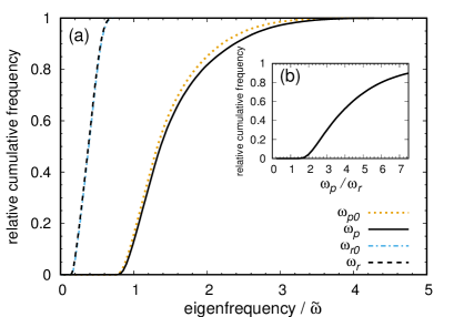
Figure 3: (color online) (a) Cumulative distributions of the pitch and the roll frequencies for the parameter set SD in Table 1; $\omega_{p}\text{~{}and~{}}\omega_{r}$ of Eq. (23) and their zeroth order approximation $\omega_{p0}$ and $\omega_{r0}$ by Eqs. (28) and (29)

are shown. The inset shows the cumulative distribution of $\omega_{p}/\omega_{r}$. The number of samples is $10^{6}$.

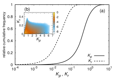
Figure 4: (color online) (a) Cumulative distributions of the asymmetric torque coefficients $K_{p}$ and $K_{r}$ for SD (Table 1). The number of samples is ${10}^{5}$. (b) A 2D color plot for the distribution of ($K_{p}$, $K_{r}$). The color code shown is in the logarithmic scale for the relative frequency $P(K_{p},\,K_{r})$, i.e., $-9\leq\log_{10}P(K_{p},\,K_{r})\leq 0$. The number of samples is $10^{8}$.

The equations of motion (10) and (11) with the contact point conditions (4) and (8) are numerically integrated by the fourth-order Runge-Kutta method with an initial condition $\bm{\omega}(0)$ and $\bm{u}(0)$. In the simulations, we take

$$\bm{u}(0)=(0,0,-1)^{t}$$ (68)

and specify $\bm{\omega}(0)$ as

$$\bm{\omega}(0)=(|\omega_{xy0}|\cos\psi,\ |\omega_{xy0}|\sin\psi,\ -n_{i})$$ (69)

in terms of $|\omega_{xy0}|$, $\psi$, and $n_{i}$. According to the simplified dynamics (47)–(49), the irrelevant mode of oscillation does not affect the dynamics sensitively as long as the relevant mode exists and the initial spin energy is much larger than the initial oscillation energy. Thus we choose $\ket{\omega(0)}=(\omega_{x0},\omega_{y0})^{t}$ in the direction of the relevant eigenmode,

$$\psi=\psi_{p}\text{ for }n_{i}>0,\quad\text{and}\quad\psi=\psi_{r}\text{ for }n_{i}<0,$$ (70)

where $\psi_{p}$ and $\psi_{r}$ are the angles of the eigenvectors $\ket{\omega_{p}}$ and $\ket{\omega_{r}}$ from the $x$-axis, respectively.

Numerical results are presented in the unit system where $M$, $a$, and

$$\tilde{t}\equiv 1/\tilde{\omega}\equiv\sqrt{a/g}$$ (71)

as units of mass, length, and time. The size of the time step for the numerical integration is taken to be $0.002\,\tilde{t}$. In numerics, we determine the time for reversal $t_{r}$ by the time at which $n=\bm{\omega}\cdot\bm{u}$ becomes zero for the first time, and they are compared with Garcia-Hubbard formulas (56) and (58); $n_{0}$ is determined as

$$\frac{\gamma n_{0}^{2}}{2}=\frac{1}{2}(\alpha\omega_{x0}^{2}+\beta\omega_{y0}^{2}+\gamma\omega_{z0}^{2}),$$ (72)

assuming $I_{\mathrm{eff}}=I_{zz}$ at $t=0$. Here the potential energy $U(\bm{u})$ is set to zero where $\bm{u}(0)=(0,0,-1)^{t}$.

The parameters used in the simulations are listed in Table 1. For the parameter set SD, the ranges are shown. When numerical results are plotted against $K_{p}$ or $K_{r}$, given by Eqs. (39) or (40), respectively, sets of parameters are chosen randomly from the ranges until resulting $K_{p}$ or $K_{r}$ falls within the range of $\pm 0.1\%$ of a target value. The ranges of SD are chosen to meet the following two conditions: (1) $0<\phi\ll\theta<1$, $\beta<\alpha$, and $|\xi|\ll 1$ and (2) the pitch frequency should be higher than the roll frequency. As argued in Sec. II.3, usual rattlebacks such as one in Fig. 1(a) satisfy these two conditions. Figure 3 shows the cumulative distributions for the eigenfrequencies $\omega_{p}$ and $\omega_{r}$, and their approximate expressions $\omega_{p0}$ and $\omega_{r0}$ for the parameter set SD; it shows $(\omega_{p}/\omega_{r})>1.3$ in accordance with the condition (2).

The parameter set GH gives $K_{p}=0.553$ and $K_{r}=0.0967$, and the distributions of $K_{p}$ and $K_{r}$ for SD are shown in Fig. 4, where one can see $K_{p}\gg K_{r}$. From Eq. (37), this corresponds to $\omega_{p}^{2}\gg\omega_{r}^{2}$, i.e., the pitch frequency is significantly faster than the roll frequency. Consequently, the time for reversal is much shorter for the unsteady direction $n_{i}>0$, where the pitching is induced, than for the steady direction $n_{i}<0$, where the rolling is induced. We denote the time for reversal for the unsteady direction as $t_{ru}$ and that for the steady direction as $t_{rs}$ when we consider a specific spinning direction.

III.3 Results

III.3.1 General behavior for the parameter set GH

Figure 5: A typical spin evolution and the corresponding $\omega_{x}$ and $\omega_{y}$ for GH (Table 1). (a) The case of the initial spin in the unsteady direction. The initial condition is specified by Eqs. (68)–(70) with $n_{i}=0.1\,\tilde{\omega}$ and $|\omega_{xy0}|=0.01\,\tilde{\omega}$. (b) The case of the initial spin in the steady direction with $n_{i}=-0.1\,\tilde{\omega}$ and $|\omega_{xy0}|=0.01\,\tilde{\omega}$. The dashed lines in (a-1) and (b-1) show Garcia and Hubbard’s solution $\overline{n}(t)$ given by Eqs. (55) and (57), respectively.

In Fig. 5 we show a typical simulation result of the time evolution of the spin $n(t)$ along with the angular velocities $\omega_{x}(t)$ and $\omega_{y}(t)$ for the parameter set GH (Table 1) in the case of the unsteady direction $n_{i}>0$ (a), and the steady direction $n_{i}<0$ (b).

Figure 5(a-1) shows that the spin $n$ changes its sign from positive to negative at $t_{ru}\approx 112\,\tilde{t}$, and Fig. 5(b-1) shows the spin $n$ changes its sign from negative to positive at $t_{rs}\approx 810\,\tilde{t}$. Garcia and Hubbard’s solutions $\overline{n}(t)$ of Eqs. (55) and (57) are shown by the dashed lines in Figs. 5(a-1) and (b-1), respectively; they are in good agreement with the numerical simulations.

The angular velocities $\omega_{x}$ and $\omega_{y}$ oscillate in much shorter time scale, and their amplitudes evolve differently depending on the spin direction. In the case of Fig. 5(a), where the positive initial spin reverses to negative, the amplitude of $\omega_{x}$ becomes large and reaches its maximum around $t_{ru}$; the amplitude of $\omega_{y}$ also becomes large around both sides of $t_{ru}$ but shows the local minimum at $t_{ru}$. Both $\omega_{x}$ and $\omega_{y}$ oscillate at the pitch frequency $\omega_{p}\approx 1.44\,\tilde{\omega}$. In the case of Fig. 5(b) where the negative spin reverses to positive, the situation is similar but the amplitude of $\omega_{y}$ reaches its maximum around $t_{rs}$, and $\omega_{x}$ and $\omega_{y}$ oscillate at the roll frequency $\omega_{r}\approx 0.602\,\tilde{\omega}$.

These features can be understood based on the analysis in the previous section as follows. The positive spin induces the pitching, which is mainly represented by $\omega_{x}$ because the eigenvector of the pitching $\ket{\omega_{p}}$ is nearly parallel to the $x$ axis, i.e., $\psi_{p}\approx-17^{\circ}$. Likewise, the negative spin induces the rolling, mainly represented by $\omega_{y}$, because $\psi_{r}\approx 88^{\circ}$. The local minima of the amplitude for $\omega_{y}$ in Fig. 5(a-3), or $\omega_{x}$ in Fig. 5(b-2), at the times for reversal are tricky; it might mean that the eigenvector of the pitching (rolling) deviates more from the $x$ axis ($y$ axis) for $\omega_{z}\neq 0$ than that for $\omega_{z}=0$; as a result, the pitching (rolling) mode has a larger projection on the $y$ axis ($x$ axis) for $\omega_{z}\neq 0$.

Note that for given $|n_{i}|$, the maximum value of $\omega_{y}$ in Fig. 5(b-3) is larger than that of $\omega_{x}$ in (a-2). This is due to $\alpha\gg\beta$; the oscillation energy around zero spin for the both cases should be the same, which gives $\alpha\overline{{\omega}_{x}^{2}}\approx\beta\overline{{\omega}_{y}^{2}}$ thus $\sqrt{\overline{\omega_{x}^{2}}}<\sqrt{\overline{\omega_{y}^{2}}}$.

III.3.2 Simulations with the parameter set SD

We present detailed results of the simulations for the ranges of the parameters given by SD in Table 1.

Unsteady initial spin direction $(n_{i}>0)$.

In this case, the system behaves basically as we expect from the Garcia-Hubbard formula unless the initial spin or oscillation is too large. Figure 6 shows the time for reversal $t_{ru}$ as a function of $K_{p}$ when spun in the unsteady direction. The results are plotted against $K_{p}$ by the procedure described in Sec. III.2.

When the initial spin $n_{i}$ is $n_{i}\lesssim 0.2\,\tilde{\omega}$ with $|\omega_{xy0}|=0.001\tilde{\omega},\,0.01\tilde{\omega}$, $t_{ru}$ is in good agreement with the Garcia-Hubbard formula $t_{rGH+}$ of Eq. (56), i.e., almost inversely proportional to $K_{p}$ with small scatter around the average. For a given $n_{i}$, as the initial oscillation amplitude $|\omega_{xy0}|$ becomes large, the standard deviations of $t_{ru}$ become large, and the average of $t_{ru}$ deviates upward from the Garcia-Hubbard formula $t_{rGH+}$, which is derived with the small amplitude approximation of $\omega_{x}$ and $\omega_{y}$. For larger $n_{i}$, $t_{rGH+}$ also underestimates $t_{ru}$, as already noted by Garcia and Hubbard Garcia and Hubbard (1988) for the parameter set GH. The underestimation can be also seen in Fig. 5(a-1), where one can see that Garcia and Hubbard’s solution $\overline{n}(t)$ of Eq. (55) changes its sign earlier than the simulation.

For $n_{i}\gtrsim 0.4\,\tilde{\omega}$, $t_{ru}$ deviates notably upward from the Garcia-Hubbard formula $t_{rGH+}$. As $n_{i}$ increases, the average of $t_{ru}$ increases and the standard deviations become large. Figure 6(b) shows a typical spin evolution with $n_{i}=0.5\,\tilde{\omega}$. The spin oscillates widely at the pitch frequency, which is qualitatively different from typical spin behaviors at small $n_{i}$ and from Garcia and Hubbard’s solution $\overline{n}(t)$ of Eq. (55) as in Fig. 5(a-1). In this region, the Garcia-Hubbard formula is no longer valid.

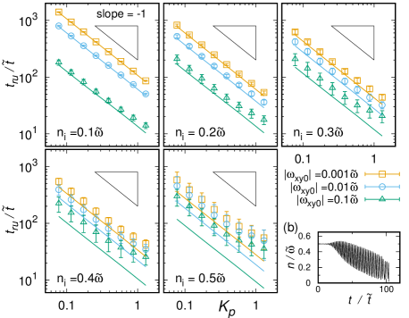
Figure 6: (color online) (a) Time for reversal of the unsteady direction $t_{ru}$ for the parameter set SD (Table 1) as a function of the asymmetric torque coefficient $K_{p}$ in the logarithmic scale. The error bars indicate one standard deviation of $1000$ samples for each data point. The solid lines are $t_{rGH+}$ given by Eq. (56), calculated using the mean values of $n_{0}$. (b) A typical spin evolution with $n_{i}=0.5\,\tilde{\omega},\ |\omega_{xy0}|=0.01\,\tilde{\omega}$. The parameter set GH is used.

Steady initial spin direction $(n_{i}<0)$.

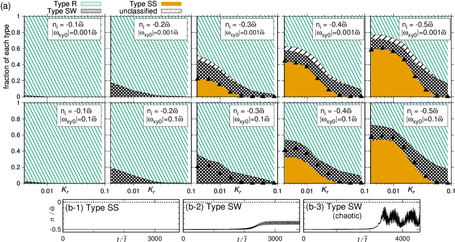
Figure 7: (color online) (a) Fractions of Types R, SS, and SW for the steady direction for eight values of $K_{r}$ with various initial conditions $|\omega_{xy0}|\text{ and }n_{i}$. Parameters are randomly chosen from SD (Table 1). The number of the samples is 1000 for each $K_{r}$. Filled triangles show the fractions of samples whose $|n_{c1}|$ is smaller than $|n_{i}|$. (b) Typical spin evolutions of a Type SS sample (b-1) and a Type SW sample (b-2), along with an example of “chaotic” oscillation (b-3) found for $K_{r}=0.0041$ with $n_{i}=-0.5\,\tilde{\omega}$.

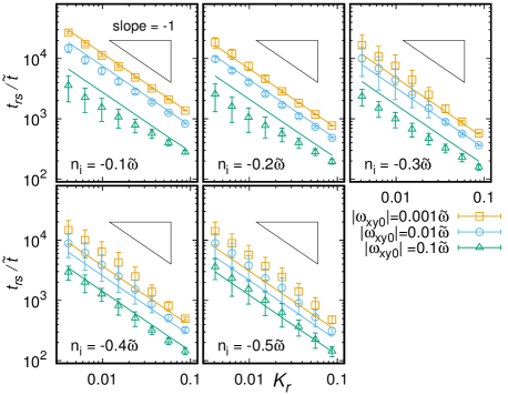
Figure 8: (color online) Time for reversal $t_{rs}$ for the steady direction as a function of $K_{r}$ in the logarithmic scale. Each data point represents the average with the standard deviation of Type R samples out of $1000$ simulations from the parameter set SD (Table 1).

Much more complicated phenomena are observed when spun in the steady direction. When the initial spin $|n_{i}|$ is small enough, the spin simply reverses as shown in Fig. 5(b-1). We call this simple reversal behavior Type R. For larger $|n_{i}|$, however, there appear some cases where the spin never reverses; in such cases there are two types of behaviors: steady spinning at $n_{ss}$ (Type SS), and spin wobbling around $n_{w}$ ($n_{ss}<n_{w}<0$, Type SW). For Type SS samples, $n_{ss}$ is slightly less than $n_{i}$, i.e., $n_{ss}<n_{i}<0$, because small initial rolling decays and its energy is converted to the spin energy. Typical spin evolutions of a Type SS sample and a Type SW sample are shown in Figs. 7(b-1) and (b-2).

Figure 7(a) shows the $K_{r}$ dependence of the fractions of Types R, SS, and SW for various initial conditions given by $n_{i}$ and $|\omega_{xy0}|$. For each sample, we wait up to $t=5t_{rGH-}$; the spin evolution is classified as Type R if it reverses. If it does not, the spin evolution is classified as Type SS if the initial rolling amplitude decays monotonously, and classified as Type SW if the spin $n$ starts wobbling by the time $5t_{rGH-}$. The other samples, in which the rolling grows slowly yet shows no visible spin change by the time $5t_{rGH-}$, are labeled “unclassified” in Fig. 7. Such samples may show spin reversal or spin wobbling if we take a much longer simulation time. Type SS appears for $|n_{i}|\gtrsim 0.3\,\tilde{\omega}$ and its fraction increases as $|n_{i}|$ increases. The fraction is larger for smaller $K_{r}$ and smaller $|\omega_{xy0}|$, i.e., $|\omega_{xy0}|=0.001\,\tilde{\omega}$. Type SW appears for $|n_{i}|\gtrsim 0.1\,\tilde{\omega}$ and its fraction is also larger for smaller $K_{r}$, but stays around $0.2$ for $|n_{i}|\gtrsim 0.4\,\tilde{\omega}$.

Figure 8 shows the $K_{r}$ dependence of $t_{rs}$ only for the samples of Type R, which shows a spin reversal behavior. For small $|n_{i}|\lesssim 0.2\,\tilde{\omega}$ with $|\omega_{xy0}|=0.01\,\tilde{\omega},0.001\,\tilde{\omega}$, $t_{rs}$ is in good agreement with Garcia-Hubbard formula $t_{rGH-}$ of Eq. (58), and the average of $t_{ru}$ is almost inversely proportional to $K_{r}$. As in the case of the unsteady direction, the standard deviations of $t_{rs}$ become large, and the average $t_{rs}$ deviates downward from $t_{rGH-}$ as initial oscillation amplitude $|\omega_{xy0}|$ becomes large. Note that $t_{rGH-}$ tends to overestimate $t_{rs}$, in contrast to the case of the unsteady direction, where $t_{rGH+}$ underestimates $t_{ru}$. This has also been noted by Garcia and Hubbard Garcia and Hubbard (1988) for the parameter set GH, and can be seen by Garcia and Hubbard’s solution $\overline{n}(t)$ in Fig. 5(b-1). For $|n_{i}|\gtrsim 0.3\,\tilde{\omega}$, one may notice the standard deviations are large for $K_{r}\ll 0.1$. In these cases, we find that some samples appear to spin stably for quite a long time, i.e., several times of $t_{rGH-}$, and then abruptly starts to reverse its sign. During the time period $t<t_{rs}$, the rolling grows much more slowly than it should as predicted by the theory in Sec. II. Such samples make both the average and standard deviation large as Fig. 8.

Next we consider the Type SS samples. There always exists a steady solution, $\bm{\omega}(0)=(0,0,\mathrm{const.})^{t}$ and $\bm{u}(0)=(0,0,-1)^{t}$, and Bondi Bondi (1986) has shown that for the steady direction, this solution is linearly stable for $n<n_{c1}<0$, where $n_{c1}(<0)$ is given by

$$n_{c1}^{2}\equiv\frac{g}{a}\frac{-(1-\theta)(1-\phi)}{2-(\theta+\phi)-(\alpha+\beta-\gamma)(\theta+\phi-2\theta\phi)}.$$ (73)

When the denominator of Eq. (73) is positive, such a threshold does not actually exist, and the steady solution is always unstable. Note that $n_{c1}$ does not depend on $\xi$.

In Fig. 7, the filled triangles show the fraction of samples whose $|n_{c1}|$ is smaller than $|n_{i}|$, which should correspond with the ratio of Type SS. For $|\omega_{xy0}|=0.001\,\tilde{\omega}$, all samples whose $|n_{c1}|$ is smaller than $|n_{i}|$ actually show Type SS behaviors and vice versa. On the other hand, for $|\omega_{xy0}|=0.1\,\tilde{\omega}$, there are some samples whose $|n_{c1}|$ is smaller than $|n_{i}|$ yet do not show Type SS behavior; for $n_{i}=-0.3\,\tilde{\omega}$, there are only several Type SS samples out of 8000 samples, which cannot be seen in Fig. 7(a), and for $|n_{i}|\gtrsim 0.4\,\tilde{\omega}$, the fractions of Type SS for $|\omega_{xy0}|=0.1\,\tilde{\omega}$ are smaller than those for $|\omega_{xy0}|=0.001\,\tilde{\omega}$. This may be because $|\omega_{xy0}|=0.1\,\tilde{\omega}$ is not small perturbation, and the spin might have escaped from the basin of attractor of Type SS behavior.

Last we consider the Type SW samples. The time when the spin starts to wobble roughly corresponds with $t_{rs}$ of Type R in Fig. 8; the center of wobbling $n_{w}$ and its amplitude vary from sample to sample. As in the case of Type R, there are some samples which start to wobble after several times of $t_{rGH-}$ where $K_{r}\ll 0.1$. Wobbling behaviors of such samples are similar to those which start wobbling around $t_{rGH-}$. We remark that there are two qualitatively different Type SW behaviors. When $|n_{i}|\lesssim 0.4\,\tilde{\omega}$, the spin of Type SW sample oscillates almost periodically. However, when $n_{i}=-0.5\,\tilde{\omega}$ and $K_{r}\ll 0.1$, we find some samples that show “chaotic” oscillations as an example shown in Fig 7(b-3).

IV Discussion

In the present work, we study the minimal model for the rattleback dynamics, i.e., a spinning rigid body with a no-slip contact ignoring any form of dissipation. We have reduced the original dynamics to the simplified dynamics (47)–(49) with the three variables. The assumptions and/or approximations used in the derivation are (1) the amplitudes of the oscillations are small, (2) the coupling between the spin and the oscillations does not depend on the spin, and (3) the time scale for the spin change is much longer than the oscillation periods. It is interesting to note that the last assumption is apparently analogous to that used in the derivation of an adiabatic invariant for some systems under slow change of an external parameter if the spin variable is regarded as a slow parameter. In the present case with this separation of time scales, the dynamics conserves the “Casimir invariant” $C_{I}$ of Eq. (51).

Our simplified dynamics can be compared with some previous works. Based on Bondi’s formulation Bondi (1986), Case and Jalal obtained the growth rates $\delta_{x}$ and $\delta_{y}$ of the pitching and the rolling amplitudes around the $x$ and $y$ axes, respectively, at a small constant spin and small skewness Case and Jalal (2014). Their results can be expressed as

$$\delta_{x}=\frac{n}{2}K_{p},\quad\delta_{y}=-\frac{n}{2}K_{r},$$ (74)

using our notations. The factor $1/2$ comes from the choice of the variables; they chose the contact point co-ordinates, while we choose the oscillation energies, which are second order quantities of their variables.

Moffatt and Tokieda Moffatt and Tokieda (2008) obtained equations for the oscillation amplitudes of pitching and rolling, $P$ and $R$, and the spinning $S$ for small spin and skewness as

$$\frac{d}{d\tau}\begin{pmatrix}P\\ R\\ S\end{pmatrix}=\begin{pmatrix}R\\ \lambda P\\ 0\end{pmatrix}\times\begin{pmatrix}P\\ R\\ S\end{pmatrix}=\begin{pmatrix}\lambda PS\\ -RS\\ R^{2}-\lambda P^{2}\end{pmatrix},$$ (75)

where $\tau$ is rescaled time, and $\lambda$ is the squared ratio of the pitch frequency to the roll frequency. Equation (75) is equivalent with Eqs. (47)–(49); again the difference comes from choice of the variables. The mathematical structures of Eq. (75) have been investigated recently in more detail by Yoshida et al. Yoshida et al. (2016) in connection with the Casimir invariant and chaotic behavior of the original dynamics.

Figure 9: Three types of spin behaviors after the first reversal period in the small spin regime with $n_{i}=0.1\tilde{\omega}$, $|\omega_{xy0}|=0.01\tilde{\omega}$. (a) A quasi-periodic behavior with the parameter set GH ($\theta=0.6429$), (b) a chaotic behavior with $\theta=0.82$, (c) a quasi-periodic behavior with a period shorter than the first one with $\theta=0.9$. All the other parameters for (b) and (c) are the same as GH. The dashed lines show the spin evolutions for the corresponding simplified dynamics, where $\overline{E}_{p}(0)=Ma^{2}[\alpha(|\omega_{xy0}|\cos\psi_{p})^{2}+\beta(|\omega_{xy0}|\sin\psi_{p})^{2}]/2$, $\overline{E}_{r}(0)=3\times 10^{-5}Ma^{2}\tilde{\omega}^{2}$, and $\overline{n}(0)=n_{i}$.

After the first round of spin reversals, our simplified dynamics (47)–(49) repeats itself and shows periodic behavior as well as the dynamics studied by Moffatt and Tokieda Eq. (75) because the system with only three variables has two conservatives, i.e., the total energy and the Casimir invariant. However, the Casimir invariant is an approximate one in the original dynamics, and invariant only under the approximations given at the beginning of this section. The Casimir “invariant” actually varies and the original system shows aperiodic behaviors.

A few examples for longer time evolutions of spin $n(t)$ are given in Fig. 9 for the system with the parameter set GH except for the curvature in the rolling direction $\theta=0.6429$ (a) for GH, $0.82$ (b), and $0.9$ (c) along with those by the corresponding simplified dynamics. The first example (a) almost shows a periodic spin reversal behavior as is expected by the simplified dynamics. It is, however, only quasi-periodic with fluctuating periodicity. The second example (b) does not show a periodic behavior; the initial spin reversal till $t/\tilde{t}\approx 100$ is nearly the same with (a), but after the time of the second spin reversal around $t/\tilde{t}\approx 3000$, it turns into chaotic, deviating from the simplified dynamics. The third example (c) may look similar to (a) but is peculiar; it shows a quasi-periodic behavior after the initial round of spin reversals, and its periodicity is much shorter than that by the simplified dynamics.

The simplified dynamics seems to work reasonably well for the case of smaller $\theta$ in (a) but fails for larger $\theta$ close to $1$ in (b) and (c). This indicates that the approximations or assumptions used to derive the simplified dynamics are not valid for the larger curvature in the rolling direction $\theta$; as the radius of curvature $1/\theta$ becomes small and close to 1, i.e., the height of the center of mass, the restoration force for the rolling oscillation becomes weak. This should result in the rolling oscillation with larger amplitude and the slower frequency, thus the assumptions (1) and (3) given at the beginning of this section may not be good enough.

The fact that the system shows a different behavior after the first round of spin reversals is reminiscent of the existence of attractors, which is normally prohibited in a conserving system by Liouville theorem. In the present system, however, the theorem is invalidated by the non-holonomic constraint due to the no-slip condition Eq. (3) . As mentioned already, the existence of strange attractors in an energy conserving system with a non-holonomic constraint has been studied by Borizov et al. Borisov et al. (2014), and chaotic behavior in the rattleback system has been discussed in connection with the Casimir invariant by Yoshida et al. Yoshida et al. (2016).

V Summary and conclusion

We have performed the theoretical analysis and numerical simulations on the minimal model of rattleback. By reformulating Garcia and Hubbard’s theory Garcia and Hubbard (1988), we obtained the concise expressions for the asymmetric torque coefficients, Eqs. (39) and (40), gave the compact proof to the fact that the pitching and the rolling generate the torques with the opposite sign, and reduced the original dynamics to the three-variable dynamics by a physically transparent procedure.

Our expressions for the asymmetric torque coefficients are equivalent to those by Garcia and Hubbard, but we explicitly elucidate that the ratio of the two coefficient for the pitching and the rolling oscillation is proportional to the squared ratio of those frequencies. Since the pitching frequency is significantly higher than that of the rolling for a typical rattleback, the time for reversal to one spin direction (or unsteady direction) is much shorter than that to the other direction (or steady direction); the spin reversal for the latter direction is not usually observed in a real rattleback due to dissipation.

The simulations on the original dynamics for various parameter sets demonstrate that Garcia-Hubbard formulas for the first spin reversal time (56) and (58) are good in the case of small initial spin and small oscillation for both the unsteady and the steady directions. The deviation from the formula is especially large for the steady direction in the fast initial spin and small $K_{r}$ regime, where the rattleback may not reverse and shows a variety of dynamics, that includes steady spinning, periodic and chaotic wobbling.

In conclusion, the rattleback is simple but shows fascinatingly rich dynamics, and keeps attracting physicists’ attention.

References

- Moffatt (2000) H. K. Moffatt, Nature (London) 404, 833 (2000).
- Moffatt and Shimomura (2002) H. K. Moffatt and Y. Shimomura, Nature (London) 416, 385 (2002).
- Jalali et al. (2015) M. A. Jalali, M. S. Sarebangholi, and M. R. Alam, Phys. Rev. E 92, 032913 (2015).
- Heckel et al. (2012) M. Heckel, P. Müller, T. Pöschel, and J. A. C. Gallas, Phys. Rev. E 86, 061310 (2012).
- Kubo et al. (2015) Y. Kubo, S. Inagaki, M. Ichikawa, and K. Yoshikawa, Phys. Rev. E 91, 052905 (2015).
- Walker (1896) G. T. Walker, Q. J. Pure Appl. Math. 28, 175 (1896).
- Bondi (1986) H. Bondi, Proc. R. Soc. Lond. A 405, 265 (1986).
- Wakasugi (2011) M. Wakasugi, Master’s thesis, Tokyo University, (2011).
- Case and Jalal (2014) W. Case and S. Jalal, Am. J. Phys. 82, 654 (2014).
- Markeev (1983) A. P. Markeev, Prikl. Mat. Mekh. 47, 575 (1983).
- Pascal (1983) M. Pascal, Prikl. Mat. Mekh. 47, 321 (1983).
- Blackowiak et al. (1997) A. D. Blackowiak, R. H. Rand, and H. Kaplan, in Proceedings of the ASME Design Engineering Technical Conferences, Sacramento, California, paper DETC97/VIB-4103 (ASME, 1997).
- Moffatt and Tokieda (2008) H. K. Moffatt and T. Tokieda, P. Roy. Soc. Edinb. A 138, 361 (2008).
- Garcia and Hubbard (1988) A. Garcia and M. Hubbard, Proc. R. Soc. Lond. A 418, 165 (1988).
- Kane and Levinson (1982) T. R. Kane and D. A. Levinson, Int. J. Nonlin. Mech. 17, 175 (1982).
- Lindberg and Longman (1983) R. E. Lindberg, Jr. and R. W. Longman, Acta Mech. 49, 81 (1983).
- Nanda et al. (2016) A. Nanda, P. Singla, and M. A. Karami, J. Sound. Vib. 369, 195 (2016).
- Borisov and Mamaev (2003) A. V. Borisov and I. S. Mamaev, Phys. Usp. 46, 393 (2003).
- Borisov et al. (2006) A. V. Borisov, A. A. Kilin, and I. S. Mamaev, Dokl. Phys. 51, 272 (2006).
- Borisov et al. (2014) A. V. Borisov, A. O. Kazakov, and S. P. Kuznetsov, Phys. Usp. 57, 453 (2014).
- Magnus (1974) K. Magnus, Z. Angew. Math. Mech. 54, 54 (1974).
- Karapetyan (1981) A. V. Karapetyan, Prikl. Mat. Mekh. 45, 42 (1981).
- Takano (2014) H. Takano, Regul. Chaotic Dyn. 19, 81 (2014).
- Zhuravlev and Klimov (2008) V. P. Zhuravlev and D. M. Klimov, Mech. Solids 43, 320 (2008).
- Awrejcewicz and Kudra (2012) J. Awrejcewicz and G. Kudra, Shock Vib. 19, 1115 (2012).
- Kudra and Awrejcewicz (2013) G. Kudra and J. Awrejcewicz, Eur. J. Mech. A-Solid 42, 358 (2013).
- Kudra and Awrejcewicz (2015) G. Kudra and J. Awrejcewicz, Acta Mech. 226, 2831 (2015).
- Goldstein et al. (2002) H. Goldstein, C. Poole, and J. Safko, Classical Mechanics, 3rd ed. (Addison Wesley, New York, 2002).
- Note (1) Note1, Note that in the atypical case of , i.e. the pitching is slower than the rolling, we have and for because by Eq. (25).
- Yoshida et al. (2016) Z. Yoshida, T. Tokieda, and P. J. Morrison, arXiv:1609.09223v1 (2016).
- Note (2) Note2, The no-slip condition should be violated in the situations where the ratio of the vertical and the inplane components of the contact force, i.e., and , exceeds the friction coefficient. The ratio becomes large when the angular momentum around changes. In the cases given in Fig. 9, its largest value is around 0.2.