Mass Loss Rates from Coronal Mass Ejections: A Predictive Theoretical Model for Solar-Type Stars

Abstract

Coronal mass ejections (CMEs) are eruptive events that cause a solar-type star to shed mass and magnetic flux. CMEs tend to occur together with flares, radio storms, and bursts of energetic particles. On the Sun, CME-related mass loss is roughly an order of magnitude less intense than that of the background solar wind. However, on other types of stars, CMEs have been proposed to carry away much more mass and energy than the time-steady wind. Earlier papers have used observed correlations between solar CMEs and flare energies, in combination with stellar flare observations, to estimate stellar CME rates. This paper sidesteps flares and attempts to calibrate a more fundamental correlation between surface-averaged magnetic fluxes and CME properties. For the Sun, there exists a power-law relationship between the magnetic filling factor and the CME kinetic energy flux, and it is generalized for use on other stars. An example prediction of the time evolution of wind/CME mass-loss rates for a solar-mass star is given. A key result is that for ages younger than about 1 Gyr (i.e., activity levels only slightly higher than the present-day Sun), the CME mass loss exceeds that of the time-steady wind. At younger ages, CMEs carry 10–100 times more mass than the wind, and such high rates may be powerful enough to dispel circumstellar disks and affect the habitability of nearby planets. The cumulative CME mass lost by the young Sun may have been as much as 1% of a solar mass.

1. Introduction

Stars never seem to be in a purely static state of mass conservation. If they are not accreting gas from the surrounding interstellar medium, they tend to be losing mass in the form of either a quasi-steady stellar wind (Lamers & Cassinelli, 1999; Romanova & Owocki, 2016) or in episodic bursts driven by a range of possible instabilities. Stellar mass loss has a significant impact on stellar and planetary evolution, and also on the larger-scale evolution of gas and dust in galaxies (e.g., Willson, 2000; Oey & Clarke, 2009; Lammer et al., 2012; See et al., 2014). The Sun, in addition to having a ubiquitous steady wind, undergoes frequent coronal mass ejections (CMEs). These are magnetically driven eruptions of plasma and electromagnetic energy that remain coherent even far into the outer heliosphere (Low, 2001; van Driel-Gesztelyi, 2005; Forbes et al., 2006; Vršnak, 2008; Schrijver, 2009; Chen, 2011; Webb & Howard, 2012; Schmieder et al., 2015). CME mass loss from other stars may be able to explain observed variability in debris disks (Osten et al., 2013) and could be powerful enough to strip away the atmospheres of of otherwise habitable exoplanets (Lammer et al., 2007; Kay et al., 2016).

Signatures of time-steady stellar winds have been detected from stars with a wide range of properties (e.g., de Jager et al., 1988; Wood, 2006; Puls et al., 2008). However, observational evidence for intermittent mass loss is still elusive. There are multiple measurements of time-variable outflows from cool stars (Houdebine et al., 1990; Cully et al., 1994; Fuhrmeister & Schmitt, 2004; Leitzinger et al., 2011; Dupree et al., 2014; Vida et al., 2016; Korhonen et al., 2017), but it is not yet clear whether these should be interpreted as magnetically driven events analogous to solar CMEs. It is possible that observing the extrasolar equivalents of Type II radio bursts (Crosley et al., 2016) or the polarization signatures of off-limb prominences (Felipe et al., 2017) could be promising avenues toward the goal of definitive exo-CME detection.

Even for the well-observed case of solar CMEs, many questions remain about how they originate and evolve. Most CMEs appear to involve the unstable expansion of twisted “flux ropes” (or some kind of highly non-potential, current-carrying magnetic field) into the heliosphere. Past attempts to winnow down the list of proposed eruption processes have depended crucially on knowledge about how the magnetic energy is stored in the non-potential regions in and around the flux rope—see, e.g., evidence presented by Antiochos et al. (1999) and Sterling et al. (2001) against the Hirayama (1974) tether-cutting scenario, or the evidence presented by Schuck (2010) against the flux injection hypothesis of Chen & Krall (2003). The true connections between temporal events such as CMEs and flares, structures such as prominences, flux ropes, and shocks, and physical processes such as reconnection, turbulence, and magnetohydrodynamic (MHD) instabilities are not yet understood.

Recent progress has been made in estimating stellar CME properties by using the Sun to normalize a correlation between the ultraviolet and X-ray energy released in flares with CME masses and kinetic energies (Aarnio et al., 2011, 2012; Drake et al., 2013; Osten & Wolk, 2015; Takahashi et al., 2016). However, this may not be the most natural way to follow the dominant energy budget in these systems. On the Sun, eruptive CMEs seem to be associated only with a subset of all X-ray flares (e.g., Nindos & Andrews, 2004; Zhang & Low, 2005). Also, despite some strong correlations between stored magnetic energy and coronal X-ray emission (Pevtsov et al., 2003; Hazra et al., 2015), the magnetic energy that is released in the form of flare radiation tends to be a very small fraction of the total. Thus, it may make more sense to use magnetic energy fluxes than it would to use flare emission as the primary scaling variable for stellar CME properties.

The objective of this paper is to extend an existing semi-analytic model of stellar wind mass-loss rates (Cranmer & Saar, 2011) to also predict CME mass-loss rates. Both models assume the overall level of magnetic activity is related to the dimensionless filling factor of strong-field regions on the stellar surface, and that the filling factor is correlated with the star’s rotation rate (i.e., the Rossby number). Section 2 of this paper shows how the Sun can be used to calibrate the correlations between magnetic filling factors and kinetic energy losses in wind/CME flows. Section 3 makes use of these correlations in building a CME mass loss model, and illustrates it with a prediction for the time evolution of mass-loss rates for a one solar mass ($M_{\odot}$) star. Lastly, Section 4 summarizes the results, discusses some wider implications of this work, and suggests future improvements.

2. Empirical Correlations with Magnetic Flux

The main conjecture of this paper is that a cool star’s magnetic field strength is a primary factor in determining its time-averaged mass loss in the form of steady wind and bursty CMEs. The Sun’s observed 11-year solar-cycle variability will be used to help determine the relationship between the kinetic energy content in the two types of outflow (Section 2.1) and the available magnetic energy (Section 2.2). The correlations themselves are discussed in Section 2.3.

2.1. Mass Loss Rates and Kinetic Energy Fluxes

For the time-steady wind, the most appropriate solar quantity to compare with stellar observations would be the total sphere-averaged mass-loss rate (i.e., accounting for all $4\pi$ steradians around the Sun). However, such complete sampling is usually not available for solar data. There is a large historical database of in situ measurements in the ecliptic plane, but Ulysses showed these are not necessarily representative of the higher latitudes (Goldstein et al., 1996). Wang (1998) produced a model-based proxy for $\dot{M}_{\rm wind}$, the sphere-averaged solar wind mass-loss rate, for solar cycles 21 and 22. This model was based on known correlations between the wind speed and density at 1 AU with the superradial expansion rate of open magnetic flux tubes. The latter can be reconstructed globally from rotation-averaged magnetograms (e.g., Wang & Sheeley, 1990).

Figure 1 shows the time dependence of the Wang (1998) derivation of $\dot{M}_{\rm wind}$ in units of $M_{\odot}$ yr^-1. At solar maximum there is a tendency for the Sun to produce slow and dense wind streams at all latitudes, as opposed to the tenuous high-speed streams that fill most of the heliospheric volume at solar minimum. Because the relative density increases in slow streams are slightly larger than the relative decreases in wind speed, the sphere-averaged mass-loss rate appears to be roughly 50% larger at solar maximum. For comparision, Figure 1 also shows an approximate correlation with sunspot number,

$$\dot{M}_{\rm wind}\,\approx\,3.5\times 10^{-17}\left(S+570\right)\,\,\,M_{\odot}\,\mbox{yr}^{-1}$$ (1)

where $S$ is the recently revised month-averaged sunspot number from the World Data Center (WDC) Sunspot Index and Long-term Solar Observations (SILSO) program (see, e.g., Clette & Lefèvre, 2016). The correlation coefficient between the data and the above fitting function is high (0.884), but it is likely that better fits can be found with additional variation of the functional form.

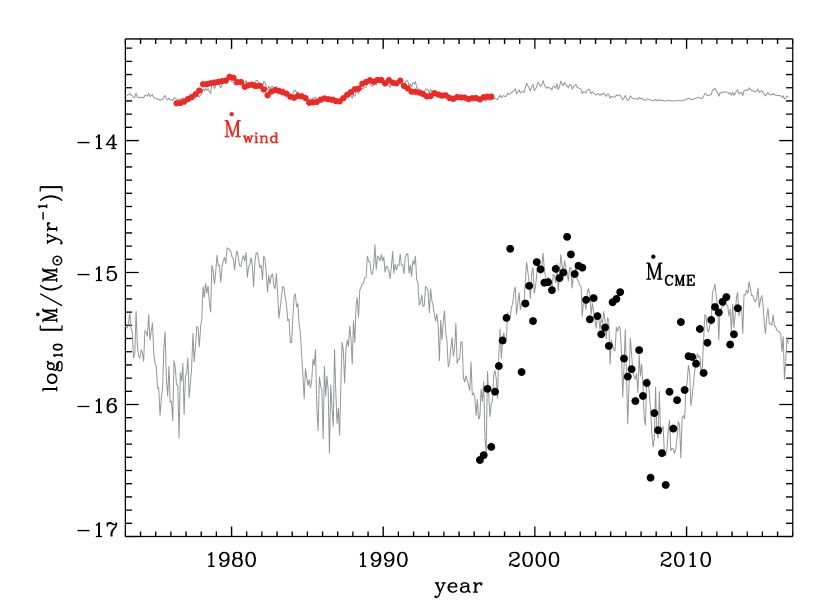
Figure 1.— Estimated time dependence of total rates of mass loss for the time-steady solar wind (Wang, 1998) (red points) and for solar CMEs from the CDAW database (black points). Also shown are approximate correlations between the mass-loss rates and specified functions of sunspot number (gray curves), given in Equations (1)–(2).

It is possible to estimate the sphere-averaged CME mass-loss rate $\dot{M}_{\rm cme}$ from visible-light coronagraph measurements. Dense CMEs show up as bright features due to the fact that optically thin Thomson scattering is linearly proportional to the line-of-sight integrated electron density. Thus, coronagraphs can be used to measure CME masses in a large fraction (but not 100%) of the volume of the extended corona and inner heliosphere.

Figure 1 shows a reconstruction of the time-variable CME mass-loss rate, assembled from the CME catalog maintained by NASA’s Coordinated Data Analysis Workshop (CDAW) data center (see, e.g., Yashiro et al., 2004; Gopalswamy et al., 2009). The most recent version of the catalog contains CME records from 1996 January to 2015 February. Out of the initial list of 25161 events, we eliminated all CMEs with marginal detections (i.e., labeled “poor” and “very poor”) and neglected all events without tabulated masses. This left a subset of 6379 CMEs between 1996 March and 2013 June.

An initial summation of these masses yielded values of $\dot{M}_{\rm cme}$ that were decidedly low in comparison to the existing CME literature. At solar maximum, the CDAW data seemed to indicate that CMEs contribute only about 3% of the background solar wind mass flux. However, earlier studies of both coronagraphic and in situ data (e.g., Hildner, 1977; Howard et al., 1985; Webb & Howard, 1994) found this number to be more like 10% to 15%. There are several possible reasons for such a discrepancy:

1. If even a fraction of the marginal CDAW events—which we removed from consideration—represented true CMEs, the initial summation would have yielded a value too low in comparison with the actual CME mass flux. The tabulated masses for these events, when they are given in the database, are likely to be highly uncertain. Nevertheless, including those masses for poor and very poor events would have increased the total CME mass in the entire database by only 19%, from $1.051\times 10^{19}$ g (without the marginal events) to $1.248\times 10^{19}$ g (with those events).

2. Standard methods of computing CME masses from coronagraph data have been found to underestimate the masses of Earth-directed “halo” events, and in some cases those CMEs could be hidden entirely behind the instrument’s occulter and thus missed completely. Howard et al. (1985) estimated that coronagraph-derived mass-loss rates may be too low by factors of 2 to 3, mainly due to these undetected events. Burkepile et al. (2004) found that “non-limb” CMEs away from the plane of the sky may have significantly underestimated masses, too.

3. CME mass flux estimates from the 1970s and 1980s may be overestimates. Vourlidas et al. (2010, 2011) noted that older visible-light instruments were generally less sensitive than modern CCD-based instruments. Thus, they were more apt to detect only the most massive CMEs. If those events were counted as “typical,” they may have contributed to larger estimates of the mean mass flux than would have been obtained from a more accurate distribution of strong and weak events.

4. Despite the above issues, Vourlidas et al. (2010, 2011) concluded that there may have been a true decline in CME mass flux from the 1970s–1980s to the 1990s–2000s.

Thus, to account for some combination of the possible underestimation effects listed above, the mass of each CME in the reduced database of 6379 events was multiplied by a constant factor of 1.5. This value may still be too low—especially if the time-averaged mass fluxes are too low by factors of 2 to 3 as suggested by Howard et al. (1985) and Vourlidas et al. (2010, 2011)—but we did not want to stray too far from the straightforward numbers given in the CDAW database. The data points in Figure 1 show the result of this adjustment. Each point is the sum of the CME masses in successive three-month intervals, starting with 1996.25–1996.50 and extending to 2013.25–2013.50. Mean rates of mass loss were computed by multiplying each summed mass by a factor of $1.5/\Delta t$, where $\Delta t=0.25$ yr. As is well-known, the solar cycle dependence in $\dot{M}_{\rm cme}$ is much stronger than for the background wind’s mass loss. The data points are plotted on top of an approximate correlation with sunspot number,

$$\dot{M}_{\rm cme}\,\approx\,5.6\times 10^{-18}\left(S+7\right)\,\,\,M_{\odot}\,\mbox{yr}^{-1}$$ (2)

and the correlation coefficient between the data and the fitting function (0.812) is only slightly lower than that of the wind. It should be noted that Equations (1) and (2) were produced for almost completely non-overlapping time periods. Also, if Vourlidas et al. (2010, 2011) were correct in their conjecture about a true secular decrease by a factor of 2 from 1970 to 2000, the above fit would not reproduce it. Nevertheless, Equations (1) and (2) are not used in the remainder of this paper and are presented only as hints for future study.

The mass-loss rates given above describe time-averaged bulk outflows of plasma from the stellar surface. A more physically meaningful way of expressing that outflow is by defining the mean kinetic energy flux $F$, which for a given component of the outflow can be expressed as

$$F(r)\,=\,\frac{1}{2}\rho u^{3}\,=\,\frac{\dot{M}u^{2}}{8\pi r^{2}}$$ (3)

where the mass density $\rho$ and radial flow speed $u$ are both functions of radial distance $r$ (see, e.g., Hammer, 1982; Hansteen & Leer, 1995; Leer et al., 1982; Withbroe, 1988; Schwadron & McComas, 2003).

The kinetic energy flux is not always the largest term in the energy budget of individual “parcels” of solar wind (Le Chat et al., 2012) or CME (Murphy et al., 2011) plasma, but it serves well to quantify the overall amount of material ejected in this form. The assumption of time-steady outflow is highlighted in the last expression in Equation (3), which presumes mass conservation,

$$\dot{M}\,=\,4\pi\rho ur^{2}\,\,\,,$$ (4)

as well as spherical symmetry far from the star. As a function of radial distance, the energy flux $F(r)$ first increases in the corona (as the flow accelerates), then it decreases in the heliosphere (as $u$ approaches a constant value and the $1/r^{2}$ term dominates). Because the goal of this paper is to relate these kinetic energy fluxes with magnetic energy fluxes (related to stellar activity and coronal heating), it simplifies matters to define a fiducial value of $F$. Thus, for convenience, the numerator of Equation (3) is specified at a sufficient distance from the star that $u$ has reached its typical terminal speed, but the denominator is specified at $r=R_{\ast}$. In other words, we define

$$F_{\rm wind}\,=\,\frac{\dot{M}_{\rm wind}u_{\rm wind}^{2}}{8\pi R_{\ast}^{2}}\,\,,$$ (5)

$$F_{\rm cme}\,=\,\frac{\dot{M}_{\rm cme}u_{\rm cme}^{2}}{8\pi R_{\ast}^{2}}$$ (6)

where $u_{\rm wind}$ and $u_{\rm cme}$ are estimates of the asymptotic flow speeds far from the star. The quantities defined above do not take on the value of $F(r)$ at any one location, but they are consistently defined as representative proxies. Alternately, one could specify these quantities as effective luminosities ($L_{\rm wind}=4\pi R_{\ast}^{2}F_{\rm wind}$, with a similar definition for $L_{\rm cme}$), but either formulation captures the major scalings with fundamental stellar properties.

2.2. Magnetic Filling Factors

A star’s overall level of magnetic activity can be measured by the properties of the magnetic field that intersects its photosphere. However, a potentially more useful quantity may be the ratio of the surface field strength to its theoretical maximum value. This maximum value is likely to be close to the so-called “equipartition” field strength that represents equal gas and magnetic pressures. Many young and active cool stars appear to have photospheric field strengths of the same order of magnitude as their equipartition fields (Saar, 1996, 2001; Reiners et al., 2009). On the Sun, the surface-averaged field tends to be several orders of magnitude smaller than the equipartition field of $\sim$1.5 kG (see below). When observed at high resolution, though, much of the Sun’s magnetic field is collected into small flux tubes that themselves exhibit nearly equipartition field strengths (e.g., Stenflo, 1973; Parker, 1978). Thus, the Sun has a small filling factor $f_{\ast}$ of fragmented strong-field regions. In the remainder of this paper, we will consider $f_{\ast}$ to be to be equivalent to the ratio of surface-averaged field strength to the equipartition field strength.

Cranmer & Saar (2011) followed the implications of assuming a causal relationship between $f_{\ast}$ and the time-steady stellar wind mass-loss rate. In order to extend that work to CME mass loss, we need to distinguish between the total filling factor $f_{\ast}$—which accounts for all magnetic fields, no matter their topology—and the filling factor of open flux $f_{\rm open}$ that counts only the field lines that connect the photosphere to the outflowing stellar wind. The latter quantity was used exclusively by Cranmer & Saar (2011), but CME rates appear to depend more on the non-potential magnetic activity in closed-field active regions. The latter should scale more like $f_{\ast}$ than $f_{\rm open}$ in environments where the total magnetic energy is dominated by these small-scale regions. For the present-day Sun, $f_{\ast}$ is usually about a factor of ten higher than $f_{\rm open}$. Figure 2(a) illustrates their inferred dependences on the solar cycle (see also Wang & Sheeley, 2002).

The solar values of $f_{\ast}$ were computed from spatially averaged surface magnetic flux densities $|B|_{\rm av}$ from two observational databases. From 1977 to 2003, full-disk measurements from the National Solar Observatory (NSO) Kitt Peak Vacuum Telescope (Livingston et al., 1976; Jones et al., 1992) were used. From 2003 to 2016, these data were supplanted by the Vector SpectroMagnetograph instrument of the Synoptic Optical Long-term Investigations of the Sun (SOLIS) facility (Keller et al., 2003; Henney et al., 2009). In a similar manner to the $\dot{M}$ data shown in Figure 1, the magnetic field data were binned into 0.25 yr averages. The filling factor $f_{\ast}$ was determined by assuming $|B|_{\rm av}=f_{\ast}B_{\ast}$. A fiducial value of $B_{\ast}=1.5$ kG was used, which is slightly higher than the standard equipartition field strength of $\sim$1.4 kG; see Section 2.1 of Cranmer & Saar (2011).

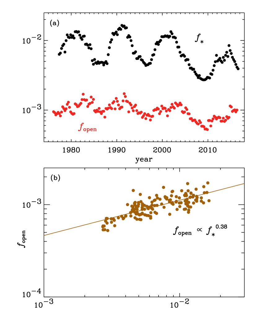
Figure 2.— (a) Time dependence of the Sun’s total magnetic filling factor $f_{\ast}$ (black points) and the filling factor of open magnetic flux $f_{\rm open}$ (red points). (b) A point-by-point comparison between $f_{\ast}$ and $f_{\rm open}$ shows that a power-law correlation reproduces much of the observed solar-cycle variability.

The filling factor of open flux $f_{\rm open}$ is not as straightforward to measure as is $f_{\ast}$. Ideally, direct measurements of the large-scale coronal magnetic field would be needed to distinguish between open and closed regions, but those are not available. In situ magnetic field measurements at 1 AU can be used, but those are usually limited to a single vantage point near the Earth. However, Ulysses showed that the radial magnetic flux $r^{2}B_{r}$ tends to be reasonably constant throughout the high- and low-latitude heliosphere (Smith & Balogh, 1995). The open field is believed to expand laterally in the low-$\beta$ (i.e., magnetic pressure dominated) corona, and neighboring flux tubes eventually reach transverse magnetic-pressure equilibrium. Thus, the open flux wants to “evenly” fill the heliospheric volume. The value of the radial flux changes with solar cycle (e.g., Svalgaard & Cliver, 2007; Smith & Balogh, 2008), but measuring it at one location in the ecliptic seems to be an adequate proxy for its mean value taken over all $4\pi$ of solid angle.

Thus, the time series of $f_{\rm open}$ values shown in Figure 2(a) was constructed from radial magnetic field strengths at 1 AU taken from the OMNI data set (King & Papitashvili, 2005). OMNI collects in situ solar wind measurements from 18 different in-ecliptic spacecraft, assembles them into a coherent and validated database, and distributes it in a range of formats at the Space Physics Data Facility (SPDF) of NASA’s Goddard Space Flight Center. Hour-averaged OMNI measurements were projected back to the solar surface assuming radial flux conservation, and the values were divided by the same equipartition field strength $B_{\ast}$ discussed above to obtain $f_{\rm open}$. To maintain continuity with the $f_{\ast}$ data, mean values of $f_{\rm open}$ were constructed for each of the three-month periods between 1976.00 and 2016.50.

As expected, $f_{\rm open}$ is smaller than $f_{\ast}$ by about an order of magnitude, but the difference is largest at solar maximum. Because both filling factors vary in phase with the solar cycle, it is possible to correlate them with one another. Figure 2(b) shows a least-squares power-law fit between the two quantities, with

$$f_{\rm open}\,\approx\,0.00645\,f_{\ast}^{0.3813}$$ (7)

indicating that the relative solar-cycle dependence of $f_{\rm open}$ is significantly muted in comparison with that of $f_{\ast}$.

2.3. Correlations with Kinetic Energy Flux Efficiencies

As stated above, the main idea of this paper is to explore the implications of a correlation between magnetic fields and the kinetic energy fluxes of stellar wind/CME outflows. A major assumption is that the Sun’s limited range of variation in quantities such as $f_{\ast}$ and $F_{\rm cme}$ over the activity cycle can be extrapolated to other stars. Specifically, we look for relationships between the filling factor $f_{\ast}$ and a similarly dimensionless ratio describing the fraction of available coronal energy that the star puts into wind/CME outflow. Those relative fractions are defined as kinetic energy flux efficiencies ${\cal E}_{\rm wind}$ and ${\cal E}_{\rm cme}$, with

$${\cal E}_{\rm wind}=\frac{F_{\rm wind}}{f_{\ast}F_{\ast}}\,\,\,\,\,\mbox{and}\,\,\,\,\,{\cal E}_{\rm cme}=\frac{F_{\rm cme}}{f_{\ast}F_{\ast}}\,\,.$$ (8)

In both cases, the denominator is a magnetically weighted convective energy flux, measured at the photosphere, that is injected into the chromosphere and corona. The quantity $F_{\ast}$ itself is taken to be the turbulent energy flux inside a representative strong-field flux tube. Cranmer & Saar (2011) extracted a fiducial solar value of $F_{\ast}=1.5\times 10^{8}$ erg cm^-2 s^-1 from published models of transverse kink-mode oscillations driven by the subsurface convection (Musielak & Ulmschneider, 2002). When the magnetic flux tubes extend above the stellar surface and expand to fill the volume, the kink-mode waves become shear Alfvén waves (see also Cranmer & van Ballegooijen, 2005).

In other words, the quantity $f_{\ast}F_{\ast}$ is assumed to be the maximum surface-averaged energy flux available for the heating and energization of plasma in CMEs and the solar wind. The efficiencies ${\cal E}_{\rm wind}$ and ${\cal E}_{\rm cme}$ describe what fractions of that maximum energy are tapped by the two types of outflow. When examining the present-day solar cycle, we assume that $F_{\ast}$ remains fixed at the value given above, and thus we implicitly assume that the dominant source of variability in wind/CME energy fluxes comes from the variability in $f_{\ast}$. Of course, when examining other stars or long-term stellar evolution, it is clear that both $f_{\ast}$ and $F_{\ast}$ must vary.

Although the use of the energy flux $F_{\ast}$ was motivated by Cranmer & Saar (2011) on the basis of successful wave/turbulence models of the solar wind, it is not completely clear that it should be used to normalize the available energy for CMEs. In many CME eruption models (see references in Section 1), the non-potential magnetic energy driving the eruption has been stored up over timescales that can be quite long compared to the underlying turbulent motions. However, the CME mass loss rates discussed in this paper are averages taken over even longer times. After averaging over multiple eruptions (and stellar rotations), the energy available to CMEs should scale with the overall strength of the stellar dynamo. It is that same dynamo that drives turbulent magnetic flux tubes up through the surface, so normalizing the overall CME energy flux to $f_{\ast}F_{\ast}$ may end up being a reasonable approximation.

Figure 3 shows how the solar energy flux efficiencies ${\cal E}_{\rm wind}$ and ${\cal E}_{\rm cme}$ vary as a function of the filling factor $f_{\ast}$. The efficiencies were computed with the following details for each case:

1. For the wind, the OMNI data at $r=1$ AU were used to compute $F(r)$ as in Equation (3). The quantity $F_{\rm wind}$, as defined in Equation (5), was then determined by mapping the measured flux down to $r=R_{\ast}$ assuming an inverse-square radial dependence. Although these data were taken from single-point measurements, the kinetic energy flux has been found to be roughly constant as a function of both latitude and solar cycle (e.g., Le Chat et al., 2012). Thus, it is likely to be a good proxy for the corresponding sphere-averaged quantity.

2. For the CMEs, the same set of CDAW events that was used for Figure 1 was analyzed to compute $F_{\rm cme}$. Here, however, the individual tabulated kinetic energies ($Mu^{2}/2$) were used instead of the masses. As above, the three-month sums were multiplied by $1.5/\Delta t$ to obtain the required time-averaged rates for input into Equation (6).

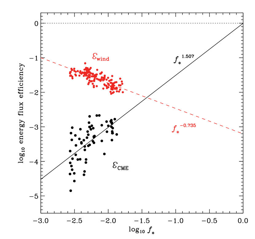
Figure 3.— Kinetic energy flux efficiencies for solar wind (${\cal E}_{\rm wind}$, red points) and for CMEs (${\cal E}_{\rm cme}$, black points) both plotted vs.  the magnetic filling factor $f_{\ast}$. Power-law fits are shown for the wind (dashed red line) and for CMEs (solid black line).

Figure 3 shows scatter plots of ${\cal E}_{\rm wind}$ and ${\cal E}_{\rm cme}$ versus $f_{\ast}$ for all three-month bins in which both abscissa and ordinate values exist. Although the Sun has only experienced about a factor of 6 variation in $f_{\ast}$ over the last few solar cycles (i.e., about 0.75 dex), the trends appear significant enough to justify fitting formulae that can be extrapolated to wider ranges of $f_{\ast}$. The following least-squares power-law fits are shown in Figure 3:

$${\cal E}_{\rm wind}\,\approx\,6.256\times 10^{-4}\,f_{\ast}^{-0.7351}$$ (9)

$${\cal E}_{\rm cme}\,\approx\,0.9955\,f_{\ast}^{1.5066}\,\,.$$ (10)

It is an interesting coincidence that the extrapolated value of ${\cal E}_{\rm cme}$ reaches a “saturation” value of 1 at nearly the same time that $f_{\ast}$ becomes equal to 1. This may be suggestive of meaningful physics behind the suggestion that the turbulent flux $F_{\ast}$ is the relevant scaling parameter for the CME energy budget. However, if taken at face value, it also implies that at $f_{\ast}\approx 1$ there may not be any remaining energy for coronal heating, X-ray emission, or flare particle production. The way stars partition the available energy into these different bins must certainly change between the low activity levels seen on the Sun and the saturated activity seen on other stars. Better theoretical models are certainly needed (see also Section 4).

Because the main results of this paper depend crucially on the correlations shown in Figure 3, some additional statistical investigation is warranted. A linear regression analysis provides standard deviations for the best-fitting values of the exponents in Equations (9)–(10). At the $1\sigma$ level, the exponents are $-0.7351\pm 0.04813$ (for the wind) and $1.5066\pm 0.2292$ (for CMEs). For the two plotted trends, the linear Pearson correlation coefficients between the data points and the fits are 0.775 (for the wind) and 0.632 (for CMEs). These values imply least-squares coefficients of determination ${\cal R}^{2}$ of 0.601 and 0.399 for the wind and CME data sets, respectively.

The above ${\cal R}^{2}$ values imply that the power-law fits “explain” only about half of the variability of the data about their respective mean values. However, it is possible to confidently reject the null hypothesis of no correlation between $f_{\ast}$ and the efficiencies ${\cal E}_{\rm wind}$ and ${\cal E}_{\rm cme}$. The classical Fisher–Snedecor $F$-test was applied to the two data sets, and the resulting ratios of explained to unexplained variance (Bevington & Robinson, 2003) were $F=233.26$ (for the wind) and $F=43.219$ (for CMEs). These correspond to probabilities $p$ for the null hypothesis of order $10^{-32}$ for the wind and $10^{-8}$ for CMEs. Of course, the $F$-test does not rule out models other than the ones given by Equations (9)–(10), but it does indicate that some meaningful correlation exists (see, however, Protassov et al., 2002). Additional goodness-of-fit calculations would be possible if the observational uncertainties of the data points were understood better, but that is beyond the scope of this paper.

Figure 3 indicates that ${\cal E}_{\rm wind}$ decreases with increasing filling factor $f_{\ast}$. In fact, this is exactly what Cranmer & Saar (2011) predicted for time-steady coronal winds. Using the standard model parameters and the approximate scaling given in Equation (45) of Cranmer & Saar (2011), the time-averaged mass-loss rate is expected to scale as $\dot{M}_{\rm wind}\propto f_{\rm open}^{5/7}$. (Note that Cranmer & Saar used the symbol $f_{\ast}$ to refer to the filling factor of open flux.) Combining that with the correlation given in Equation (7) of this paper, this is equivalent to $\dot{M}_{\rm wind}\propto f_{\ast}^{0.2724}$. For variations over our solar cycle, most of the fundamental stellar parameters (e.g., $R_{\ast}$, $F_{\ast}$, and $u_{\rm wind}\approx V_{\rm esc}$) are held fixed, so the predicted scaling would be $F_{\rm wind}\propto f_{\ast}^{0.2724}$, and thus ${\cal E}_{\rm wind}\propto f_{\ast}^{-0.7276}$. This exponent is extremely close to the least-squares value given in Equation (9).

Lastly, it is interesting to note that the two curves in Figure 3 appear to cross one another when $f_{\ast}\approx 0.037$. This indicates that activity levels only slightly higher than the present-day Sun’s may start to show CMEs with comparable mass loss as their time-steady winds.

3. Evolution of a Solar-Type Star

The correlations noted above can be used to construct semi-empirical predictions for both $\dot{M}_{\rm wind}$ and $\dot{M}_{\rm cme}$ as functions of fundamental stellar parameters. A particularly illustrative case is the evolutionary track of a star having $M_{\ast}=1\,M_{\odot}$. There is evidence that the “young Sun” produced a much denser and more energetic gas outflow than it does today, which was likely to have been important to early planetary evolution (e.g., Wood, 2006; Güdel, 2007; Lammer et al., 2012; Johnstone et al., 2015). Was this outflow dominated by CMEs?

3.1. Activity-Rotation Relations

For many cool stars, there is a significant correlation between the overall activity level—measured via a range of chromospheric and coronal emission diagnostics—and the rotation rate (Noyes et al., 1984; Pizzolato et al., 2003; Mamajek & Hillenbrand, 2008; Wright et al., 2011). As direct measurements of stellar magnetic fields have become available, similar correlations for the surface-averaged field strength (essentially $f_{\ast}B_{\ast}$) and $f_{\ast}$ itself have also emerged (Saar, 1991, 2001; Montesinos & Jordan, 1993; Cuntz et al., 1998; Marsden et al., 2014; Folsom et al., 2016). Although there has been a great deal of work done to understand these correlations as the manifestation of a stellar MHD dynamo (e.g., Dobler, 2005; Christensen, 2010; Brun et al., 2015), in this paper they are treated as purely empirical scaling relations. In other words, we assume $f_{\ast}$ can be specified as some function of the stellar rotation rate.

Cranmer & Saar (2011) collected a number of $f_{\ast}$ measurements for cool stars and parameterized their dependence on the so-called Rossby number Ro, the ratio of the rotation period to a convective overturning timescale. Figure 4 shows two approximate “envelope” curves that were found to encompass most of the data points. These curves were parameterized as follows,

$$f_{\rm min}\,=\,\frac{0.5}{[1+(x/0.16)^{2.6}]^{1.3}}\,\,,$$ (11)

$$f_{\rm max}\,=\,\frac{1}{1+(x/0.31)^{2.5}}$$ (12)

where $x=\mbox{Ro}/\mbox{Ro}_{\odot}$ and the Sun’s present-day Rossby number was calibrated to be $\mbox{Ro}_{\odot}=1.96$. See Equation (36) of Cranmer & Saar (2011) for additional details about calculating Ro and interpreting the data.

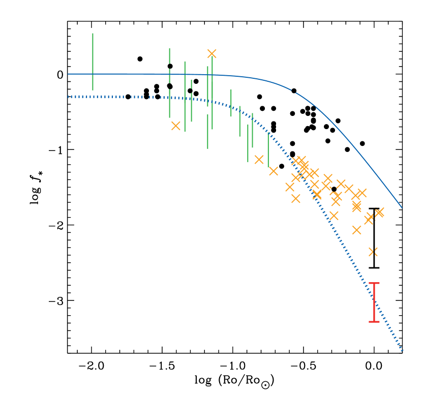
Figure 4.— Comparison of observationally inferred magnetic filling factors with Rossby number, normalized by the Sun’s present-day Rossby number. Data points are from Cranmer & Saar (2011) (black solid points), Marsden et al. (2014) (orange crosses), and Folsom et al. (2016) (green lines). Fitting functions for $f_{\rm min}$ (blue dotted curve) and $f_{\rm max}$ (blue solid curve), as well as the present-day solar-cycle variation of the Sun’s $f_{\ast}$ (black strut) and $f_{\rm open}$ (red strut) are also shown.

The number of stars used by Cranmer & Saar (2011) was quite limited in comparison with more recent observational work to measure cool-star magnetic fields. For example, the Zeeman Doppler Imaging (ZDI) technique has provided spatially resolved maps of vector surface fields on dozens of stars (e.g., Donati et al., 2012; Vidotto et al., 2014; See et al., 2015; Folsom et al., 2016). However, one must be careful in interpreting ZDI field strengths, because the technique is not sensitive to small-scale regions with balanced positive and negative polarities. Thus, ZDI field strengths are likely to be underestimates of the true surface fluxes and filling factors.

To help quantify how flux much is missed by cool-star ZDI measurements, Vidotto (2016) and Jardine et al. (2017) processed high-resolution solar data in a similar manner as in standard ZDI analyses (i.e., they kept the power only from low-order spherical-harmonic $\ell$ indices). The low-order fields do a reasonable job of reconstructing the open flux, but not the total closed flux that contributes to $f_{\ast}$. The example computed by Vidotto (2016), from the rising phase of solar cycle 24, shows that limiting $\ell$ to the ZDI-sensitive values below $\sim$10 captures only a few percent of the Sun’s magnetic energy. In this case, multiplying the ZDI surface-averaged field strength $\langle B\rangle$ by factors of at least 5–10 would reproduce the actual mean field strength. However, Jardine et al. (2017) found that during spot-free conditions more appropriate for solar minimum, ZDI may capture more than half of the total magnetic flux. This indicates a correction factor $\lesssim 2$ for low-activity times. Thus, it appears that multiplying the ZDI-derived value of $\langle B\rangle$ by a correction factor $>1$ goes in the right direction, but the uncertainty on this correction factor is large.

Observational estimates of mean field strengths $\langle B\rangle$ have been extracted from two independent surveys: (1) Marsden et al. (2014) reported mean longitudinal field strengths for 67 stars; i.e., line-of-sight components of the magnetic field, averaged over the stellar disk. (2) Folsom et al. (2016) reported the strengths of individual ZDI multipole components for 15 stars, along with the surface-averaged field $\langle B\rangle$. The inferred values of $\langle B\rangle$ were converted into $f_{\ast}$ by multiplying by a constant correction factor and dividing by $B_{\ast}$ values computed from each star’s fundamental parameters, as in Cranmer & Saar (2011). A correction factor of 7—more appropriate for solar maximum fields than solar minimum fields—was chosen because most of these stars are more active than the Sun, and thus are likely to be more similar to the most active phases of the present-day solar cycle. For the data taken from Marsden et al. (2014), Figure 4 shows only stars that had relative uncertainties in $\langle B\rangle$ less than 10%. For Folsom et al. (2016), we plotted each star as a vertical bar that extends from its ZDI-derived value of $\langle B\rangle$ up to its peak value of surface $B$ measured over rotational phase. The Rossby numbers corresponding to these data points were taken from their respective papers. Recomputing them using the Cranmer & Saar (2011) method does not produce any substantial difference in the appearance of Figure 4.

The corrected points from Marsden et al. (2014) and Folsom et al. (2016) fit roughly inside the envelope defined by the $f_{\rm min}$ and $f_{\rm max}$ curves at large and small Rossby numbers, but the agreement is worse at intermediate values. The ZDI-derived data appear to follow a shallow power-law dependence on Rossby number, with roughly $f_{\ast}\propto\mbox{Ro}^{-1.3}$. This stands in contrast to the steeper limiting slopes of $f_{\rm max}\propto\mbox{Ro}^{-2.5}$ and $f_{\rm min}\propto\mbox{Ro}^{-3.4}$ in the limit of slow rotation ($\mbox{Ro}\gtrsim 1$). Of course, using a single constant correction factor of 7 for the ZDI data is not likely to be valid across a large range of activity levels. It is possible the different slopes could be reconciled with one another if a more physically motivated correction procedure was used. The implications of the different slopes on the age dependence of CME mass-loss rate are discussed below.

3.2. Predicted Mass Loss History

In order to apply the scaling relations defined above, the effective velocities $u_{\rm wind}$ and $u_{\rm cme}$ need to be specified. Cranmer & Saar (2011) assumed that $u_{\rm wind}=V_{\rm esc}$, the surface escape speed, which for the present-day Sun is 618 km s^-1. Observed CME speeds tend to be comparable to solar wind speeds, but the solar cycle distribution is broader and more skewed to higher values than that of $u_{\rm wind}$ (see also St. Cyr et al., 2000; Owens & Cargill, 2004; Yurchyshyn et al., 2005). The CDAW catalog contains representative coronal values of $u_{\rm cme}$ for each event. For the CMEs included in Figures 1 and 3 above, the distribution of speeds is similarly broad and skewed as has been reported in the literature. The mean and median values are 449 and 402 km s^-1, respectively, and the standard deviation is 224 km s^-1. Although there is a hint of a trend with solar activity (with larger values at solar maximum), we adopt the simple relationship $u_{\rm cme}\approx 0.7V_{\rm esc}$ that is consistent with the present-day mean and median.

Assembling together Equations (6), (8), (10), and the above scaling for $u_{\rm cme}$, the mean CME mass-loss rate is given by

$$\dot{M}_{\rm cme}\,\approx\,51.06\left(\frac{F_{\ast}R_{\ast}^{2}}{V_{\rm esc}^{2}}\right)f_{\ast}^{2.5066}\,\,\,.$$ (13)

Instead of using the age dependence implied in the limiting curves of $f_{\rm min}$ and $f_{\rm max}$, we estimated two intermediate tracks that agree with present-day solar minimum and maximum activity levels. These tracks can be specified by interpolating between the two envelope curves defined by Equations (11) and (12), with a new effective filling factor defined as

$$f_{\rm eff}\,=\,f_{\rm min}^{1-\delta}f_{\rm max}^{\delta}\,\,.$$ (14)

The parameter $\delta$ indicates the fractional extent to which an intermediate curve spans the gap between $f_{\rm min}$ (i.e., $\delta=0$) and $f_{\rm max}$ (i.e., $\delta=1$). Curves that intercept the current range of solar activity levels correspond roughly to $\delta=0.30$ (present-day solar minimum $f_{\ast}\approx 0.003$) and $\delta=0.63$ (present-day solar maximum $f_{\ast}\approx 0.012$).

Figure 5 shows the evolutionary history of steady wind and CME mass-loss rates for a solar-mass star. Evolutionary tracks for stellar radius, luminosity, and effective temperature as a function of age $t$ were taken from the tabulated $1\,M_{\odot}$ model of Pietrinferni et al. (2004). The rotational evolution was taken from the model of Denissenkov et al. (2010). These parameters were used to compute the quantities on the right-hand side of Equation (13) using the formulae given by Cranmer & Saar (2011). As described above, the two plotted curves for $\dot{M}_{\rm cme}$ were computed with $\delta=0.30$ and 0.63.

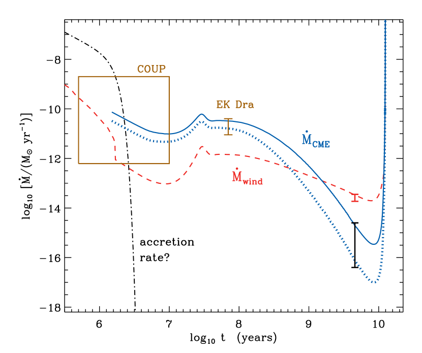
Figure 5.— Theoretical predictions of the mass-loss evolution of a $1\,M_{\odot}$ star, showing the time-steady $\dot{M}_{\rm wind}$ (red dashed curve), limiting values of $\dot{M}_{\rm cme}$ for $\delta=0.30$ (blue dotted curve) and $\delta=0.63$ (blue solid curve), and an order-of-magnitude estimate of the young-Sun accretion rate (black dot-dashed curve). Also shown are present-day measurements for the mass-loss rates (red and black error bars) and flare-based estimates of $\dot{M}_{\rm cme}$ for EK Dra (brown error bar) and T Tauri stars from the COUP database (brown rectangle).

Figure 5 also contains estimates for the time-steady solar wind mass-loss rate $\dot{M}_{\rm wind}$ and the mean gas accretion rate during the T Tauri phase. The curve for $\dot{M}_{\rm wind}$ contains two parts: (1) for $\log t\gtrsim 6.2$, it is identical to that shown in Figure 14 of Cranmer & Saar (2011), and (2) for $\log t<6.2$, the larger accretion-powered mass-loss rate predicted by Cranmer (2008) is shown instead. The accretion rate shown in Figure 5 is a simplistic convolution of a power law decline of $t^{-1.5}$ at young ages (see Hartmann et al., 1998) and a rapid exponential decay that takes hold after a few Myr (i.e., when the primordial gas disk is expected to dissipate). The accretion rate is shown only for relative comparison with the various predicted outflow components.

A major conclusion to be drawn from Figure 5 is that, at ages younger than about $\sim$1 Gyr, the CME mass loss from a $1\,M_{\odot}$ star exceeds that from the more steady wind that is accelerated along large-scale open field lines. Over the first 0.3 Gyr of a solar-mass star’s lifetime (i.e., $\log t\lesssim 8.5$), this model predicts that $\dot{M}_{\rm cme}$ may exceed $\dot{M}_{\rm wind}$ by factors of 10 to 100. It should also be noted that between $\sim$0.3 Gyr and the present, $\dot{M}_{\rm cme}$ drops off roughly as $t^{-3}$ to $t^{-4}$. This comes mainly from the $f_{\ast}^{2.5}$ dependence in Equation (13), in combination with the rough scalings $f_{\ast}\propto\mbox{Ro}^{-3}$ and $\mbox{Ro}\propto t^{0.5}$. If, however, the shallower power-law $f_{\ast}\propto\mbox{Ro}^{-1.3}$ implied by the ZDI data is valid (Marsden et al., 2014; Folsom et al., 2016), this would imply a similarly shallow age dependence of $\dot{M}_{\rm cme}\propto t^{-1.5}$ to $t^{-2}$. If the CME mass-loss rate is normalized at the present-day values, this alternate scaling would mean that $\dot{M}_{\rm cme}$ would be much lower at younger ages.

For additional observational context, Figure 5 shows two example flare-based inferences of $\dot{M}_{\rm cme}$ for young stars. The large rectangle indicates ages and mass-loss uncertainty limits for the T Tauri stars measured by the Chandra Orion Ultradeep Project (COUP). The ages were estimated by Preibisch & Feigelson (2005) and the CME mass-loss rates were estimated by Aarnio et al. (2012). Also shown is a smaller range of uncertainties for EK Dra, a young solar analog whose flaring has been observed extensively. For this star, Osten & Wolk (2015) estimated the plotted range of values for $\dot{M}_{\rm cme}$; the agreement with the model-based curves is rather good. This agreement may be indirect evidence in favor of the steeper relationship between Rossby number and magnetic filling factor ($f_{\ast}\propto\mbox{Ro}^{-2.5}$ to $\mbox{Ro}^{-3.4}$) embodied in the $f_{\rm min}$ and $f_{\rm max}$ curves in Figure 4.

4. Discussion and Conclusions

This paper has shown the existence of correlations between the Sun’s surface-averaged magnetic flux and the mean kinetic energy fluxes of the solar wind and CMEs. By framing these as correlations between dimensionless filling factors and efficiencies, the goal was to generalize them to be able to predict CME mass-loss rates for cool stars over a wide range of ages and fundamental parameters. The resulting prediction for the time evolution of a solar-mass star with solar composition (Figure 5) showed good agreement with independent estimates of $\dot{M}_{\rm cme}$ for other young solar analogues. During much of the first billion years of the model 1 $M_{\odot}$ star’s existence, the predicted CME mass-loss rate is roughly an order of magnitude higher than that of the time-steady wind. The present-day reversal of that situation is facilitated by a substantially faster time-decay for $\dot{M}_{\rm cme}$ than for $\dot{M}_{\rm wind}$.

This work built on earlier theoretical models of time-steady solar wind scaling relations (Cranmer & Saar, 2011) and on empirical correlations between CME properties and high-energy flare emissions (e.g., Aarnio et al., 2012; Drake et al., 2013; Osten & Wolk, 2015). Although it is likely that the magnetic properties of a star are more fundamental (i.e., they are what drive the flare and CME properties), it is also undeniable that they are much more difficult to observe than, say, flare light curves. Another potentially useful observable may be total spot coverage, which may be measurable from stellar light curves (Strassmeier, 2009) and has been shown—at least for individual sunspot groups—to be correlated with flare X-ray flux (Sammis et al., 2000). Thus, it would be highly beneficial to build theoretical models that self-consistently combine all four major aspects of episodic variability (magnetic fields, photospheric spots, flares, and CMEs). This would allow us to validate the existing correlations and specify how far the parameters can be extrapolated for other stars.

Predictive models of wind/CME mass loss can be used to help constrain models of stellar rotational evolution, primordial disk depletion, and particle ablation of planetary atmospheres. Drake et al. (2013) also suggested that CME mass loss may help explain the so-called “faint young Sun problem,” in which the young Earth appears to have had liquid water even though the Sun’s luminosity would have implied global temperatures below the freezing point (Sagan & Mullen, 1972; Feulner, 2012). One possible solution to the problem is that the young Sun may have been more massive (and thus more luminous) than standard solar models predict. If the Sun had lost roughly 3% to 7% of its initial mass over its first few Gyr (Sackmann & Boothroyd, 2003; Minton & Malhotra, 2007), its early luminosity may have been high enough to resolve the problem.

Although the model presented in this paper has a relatively high cumulative mass loss due to CMEs, it does not appear to be enough to solve the faint young Sun problem. The curves shown in Figure 5 were integrated in time between $\log t=6.17$ and 9.66. The mass lost by the time-steady wind is about 0.085% of a solar mass. The masses corresponding to the two CME curves are 0.33% (minimum) and 0.87% (maximum) of a solar mass. Because these numbers are dominated by long-term behavior over timescales of 0.1–1 Gyr, they are insensitive to the exact choice of starting age. The active-Sun number of about 1% agrees with the flare-based prediction of Katsova & Livshits (2014), but it appears insufficient to raise the young Sun’s luminosity enough to solve the overall freezing problem.

Both the data and models presented in this paper can be improved in several ways to increase the accuracy of the results. For example, a more comprehensive accounting of coronagraph-derived CME masses and kinetic energies should be performed in order to reduce the existing uncertainties at the level of factors of 2–3. Also, the derivation of magnetic filling factors $f_{\ast}$ from ZDI measurements—and reconciling these data with the Zeeman-broadened filling factors from unpolarized stellar spectra (Saar, 2001)—needs to be improved. Lastly, the relatively large predicted values of $\dot{M}_{\rm cme}$ discussed above should be reconciled with some measurements that failed to detect such high rates of mass loss (e.g., Lim & White, 1996; Wood et al., 2014). Drake et al. (2017) suggested that on very active stars, some CMEs may be trapped or “stalled” beneath large-scale magnetic loops that exert substantial magnetic tension on underlying unstable prominences. Their associated flares may still appear in light curves, but their mass may be recycled back down to the coronal base.

For young T Tauri stars still experiencing active accretion, Cranmer (2008, 2009) showed that photospheric MHD turbulence—which is likely to drive coronal activity—can be produced by two possible mechanisms: convective motions (from below) and impacts from “blobs” flowing along magnetospheric accretion streams (from above). As mentioned above, it is possible that for ages less than about 1 Myr, the second source of turbulence may cause $\dot{M}_{\rm cme}$ to jump up by an order of magnitude in the same way that $\dot{M}_{\rm wind}$ does in the Cranmer (2008, 2009) models. This would increase $\dot{M}_{\rm cme}$ to about 10% of the accretion rate, which appears to be a necessary condition for enabling the observed wind-torque spindown of solar-type stars (Matt & Pudritz, 2005, 2008).

A final example of the broader importance of studying CME mass loss on active stars is their potential importance to regulating stellar dynamos. It has been proposed that CMEs help shed one cycle’s dominant magnetic helicity, which would otherwise build up in the convection zone, to make room for the next cycle’s opposite helicity (Blackman & Field, 2000; Low, 2001; Brandenburg, 2007). These insights came from studying the modern-day solar case, for which CMEs only make up a small fraction of the mass loss. However, in cases of CME-dominated mass loss on active stars, the resulting dynamo may operate in qualitatively different ways than that of the present-day Sun.

References

- Aarnio et al. (2012) Aarnio, A. N., Matt, S. P., & Stassun, K. G. 2012, ApJ, 760, 9
- Aarnio et al. (2011) Aarnio, A. N., Stassun, K. G., Hughes, W. J., & McGregor, S. L. 2011, Sol. Phys., 268, 195
- Antiochos et al. (1999) Antiochos, S. K., DeVore, C. R., & Klimchuk, J. 1999, ApJ, 510, 485
- Bevington & Robinson (2003) Bevington, P. R., & Robinson, D. K. 2003, Data Reduction and Error Analysis for the Physical Sciences, 3rd ed. (Boston: McGraw-Hill)
- Blackman & Field (2000) Blackman, E. G., & Field, G. B. 2000, MNRAS, 318, 724
- Brandenburg (2007) Brandenburg, A. 2007, Highlights Astron., 14, 291
- Brun et al. (2015) Brun, A. S., García, R. A., Houdek, G., Nandy, D., & Pinsonneault, M. 2015, Space Sci. Rev., 196, 303
- Burkepile et al. (2004) Burkepile, J. T., Hundhausen, A. J., Stanger, A. L., et al. 2004, J. Geophys. Res., 109, A03103
- Chen & Krall (2003) Chen, J., & Krall, J. 2003, J. Geophys. Res., 108, 1410
- Chen (2011) Chen, P. F. 2011, LRSP, 8, 1
- Christensen (2010) Christensen, U. R. 2010, Space Sci. Rev., 152, 565
- Clette & Lefèvre (2016) Clette, F., & Lefèvre, L. 2016, Sol. Phys., 291, 2629
- Cranmer (2008) Cranmer, S. R. 2008, ApJ, 689, 316
- Cranmer (2009) Cranmer, S. R. 2009, ApJ, 706, 824
- Cranmer & Saar (2011) Cranmer, S. R., & Saar, S. H. 2011, ApJ, 741, 54
- Cranmer & van Ballegooijen (2005) Cranmer, S. R., & van Ballegooijen, A. A. 2005, ApJS, 156, 265
- Crosley et al. (2016) Crosley, M. K., Osten, R. A., Broderick, J. W., et al. 2016, ApJ, 830, 24
- Cully et al. (1994) Cully, S. L., Fisher, G. H., Abbott, M. J., & Siegmund, O. H. W. 1994, ApJ, 435, 449
- Cuntz et al. (1998) Cuntz, M., Ulmschneider, P., & Musielak, Z. E. 1998, ApJ, 493, L117
- de Jager et al. (1988) de Jager, C., Nieuwenhuijzen, H., & van der Hucht, K. A. 1988, A&AS, 72, 259
- Denissenkov et al. (2010) Denissenkov, P. A., Pinsonneault, M., Terndrup, D. M., & Newsham, G. 2010, ApJ, 716, 1269
- Dobler (2005) Dobler, W. 2005, Astron. Nachr., 326, 254
- Donati et al. (2012) Donati, J.-F., Gregory, S. G., Alencar, S. H. P., et al. 2012, MNRAS, 425, 2948
- Drake et al. (2013) Drake, J. J., Cohen, O., Yashiro, S., & Gopalswamy, N. 2013, ApJ, 764, 170
- Drake et al. (2017) Drake, J. J., Cohen, O., Garraffo, C., & Kashyap, V. 2017, in IAU Symp. 320, Solar and Stellar Flares and Their Effects on Planets, ed. A. Kosovichev, S. Hawley, P. Heinzel, in press, arXiv:1610.05185
- Dupree et al. (2014) Dupree, A. K., Brickhouse, N. S., Cranmer, S. R., et al. 2014, ApJ, 789, 27
- Felipe et al. (2017) Felipe, T., Martínez González, M. J., & Asensio Ramos, A. 2017, MNRAS, 465, 1654
- Feulner (2012) Feulner, G. 2012, Rev. Geophys., 50, RG2006
- Folsom et al. (2016) Folsom, C. P., Petit, P., Bouvier, J., et al. 2016, MNRAS, 457, 580
- Forbes et al. (2006) Forbes, T. G., Linker, J. A., Chen, J., et al. 2006, Space Sci. Rev., 123, 251
- Fuhrmeister & Schmitt (2004) Fuhrmeister, B., & Schmitt, J. H. M. M. 2004, A&A, 420, 1079
- Goldstein et al. (1996) Goldstein, B. E., Neugebauer, M., Phillips, J. L., et al. 1996, A&A, 316, 296
- Gopalswamy et al. (2009) Gopalswamy, N., Yashiro, S., Michalek, G., et al. 2009, EM&P, 104, 295
- Güdel (2007) Güdel, M. 2007, Living Rev. Solar Phys., 4, 3
- Hammer (1982) Hammer, R. 1982, ApJ, 259, 767
- Hansteen & Leer (1995) Hansteen, V. H., & Leer, E. 1995, J. Geophys. Res., 100, 21577
- Hazra et al. (2015) Hazra, S., Nandy, D., & Ravindra, B. 2015, Sol. Phys., 290, 771
- Henney et al. (2009) Henney, C. J., Keller, C. U., Harvey, J. W., et al. 2009, in ASP Conf. Proc. 405, Solar Polarization 5, ed. S. V. Berdyugina, K. N. Nagendra, R. Ramelli (San Francisco: ASP), 47
- Hartmann et al. (1998) Hartmann, L., Calvet, N., Gullbring, E., & D’Alessio, P. 1998, ApJ, 495, 385
- Hildner (1977) Hildner, E. 1977, in Study of Travelling Interplanetary Phenomena, ed. M. Shea, D. Smart, S. Wu (Dordrecht: Reidel), 3
- Hirayama (1974) Hirayama, T. 1974, Sol. Phys., 34, 323
- Houdebine et al. (1990) Houdebine, E. R., Foing, B. H., & Rodono, M. 1990, A&A, 238, 249
- Howard et al. (1985) Howard, R. A., Sheeley, N. R., Jr., Koomen, M. J., & Michels, D. J. 1985, J. Geophys. Res., 90, 8173
- Jardine et al. (2017) Jardine, M., Vidotto, A. A., & See, V. 2017, MNRAS, 465, L25
- Johnstone et al. (2015) Johnstone, C. P., Güdel, M., Brott, I., & Lüftinger, T. 2015, A&A, 577, A28
- Jones et al. (1992) Jones, H. P., Duvall, T. L., Harvey, J. W., et al. 1992, Sol. Phys., 139, 211
- Katsova & Livshits (2014) Katsova, M. M., & Livshits, M. A. 2014, Ge&Ae, 54, 982
- Kay et al. (2016) Kay, C., Opher, M., & Kornbleuth, M. 2016, ApJ, 826, 195
- Keller et al. (2003) Keller, C. U., Harvey, J. W., & the SOLIS Team 2003, in ASP Conf. Proc. 307, Solar Polarization, ed. J. Trujillo-Bueno & J. Sanchez Almeida (San Francisco: ASP), 13
- King & Papitashvili (2005) King, J. H., & Papitashvili, N. E. 2005, J. Geophys. Res., 110, A02104
- Korhonen et al. (2017) Korhonen, H., Vida, K., Leitzinger, M., Odert, P., & Kovács, O. E. 2017, in IAU Symp. 328, Living Around Active Stars, ed. D. Nandi, A. Valio, P. Petit, in press, arXiv:1612.06643
- Lamers & Cassinelli (1999) Lamers, H. J. G. L. M., & Cassinelli, J. P. 1999, Introduction to Stellar Winds (Cambridge: Cambridge University Press)
- Lammer et al. (2012) Lammer, H., Güdel, M., Kulikov, Y., et al. 2012, EP&S, 64, 179
- Lammer et al. (2007) Lammer, H., Lichtenegger, H. I. M., Kulikov, Y. N., et al. 2007, AsBio, 7, 185
- Le Chat et al. (2012) Le Chat, G., Issautier, K., & Meyer-Vernet, N. 2012, Sol. Phys., 279, 197
- Leer et al. (1982) Leer, E., Holzer, T. E., & Flå, T. 1982, Space Sci. Rev., 33, 161
- Leitzinger et al. (2011) Leitzinger, M., Odert, P., Ribas, I., et al. 2011, A&A, 536, A62
- Lim & White (1996) Lim, J., & White, S. M. 1996, ApJ, 462, L91
- Livingston et al. (1976) Livingston, W. C., Harvey, J., Pierce, A. K., et al. 1976, Applied Optics, 15, 33
- Low (2001) Low, B. C. 2001, J. Geophys. Res., 106, 25141
- Mamajek & Hillenbrand (2008) Mamajek, E. E., & Hillenbrand, L. A. 2008, ApJ, 687, 1264
- Marsden et al. (2014) Marsden, S. C., Petit, P., Jeffers, S. V., et al. 2014, MNRAS, 444, 3517
- Matt & Pudritz (2005) Matt, S., & Pudritz, R. E. 2005, ApJ, 632, L135
- Matt & Pudritz (2008) Matt, S., & Pudritz, R. E. 2008, ApJ, 681, 391
- Minton & Malhotra (2007) Minton, D. A., & Malhotra, R. 2007, ApJ, 660, 1700
- Montesinos & Jordan (1993) Montesinos, B., & Jordan, C. 1993, MNRAS, 264, 900
- Murphy et al. (2011) Murphy, N. A., Raymond, J. C., & Korreck, K. E. 2011, ApJ, 735, 17
- Musielak & Ulmschneider (2002) Musielak, Z. E., & Ulmschneider, P. 2002, A&A, 386, 606
- Nindos & Andrews (2004) Nindos, A., & Andrews, M. D. 2004, ApJ, 616, L175
- Noyes et al. (1984) Noyes, R. W., Hartmann, L. W., Baliunas, S. L., et al. 1984, ApJ, 279, 763
- Oey & Clarke (2009) Oey, M. S., & Clarke, C. J. 2009, in Massive Stars: From Pop III and GRBs to the Milky Way, STScI Symp. Ser. 20, ed. M. Livio & E. Villaver (Cambridge: Cambridge University Press), 74
- Osten et al. (2013) Osten, R. A., Livio, M., Lubow, S., et al. 2013, ApJ, 765, L44
- Osten & Wolk (2015) Osten, R. A., & Wolk, S. J. 2015, ApJ, 809, 79
- Owens & Cargill (2004) Owens, M., & Cargill, P. 2004, Ann. Geophys., 22, 661
- Parker (1978) Parker, E. N. 1978, ApJ, 221, 368
- Pevtsov et al. (2003) Pevtsov, A. A., Fisher, G. H., Acton, L. W., et al. 2003, ApJ, 598, 1387
- Pietrinferni et al. (2004) Pietrinferni, A., Cassisi, S., Salaris, M., & Castelli, F. 2004, ApJ, 612, 168
- Pizzolato et al. (2003) Pizzolato, N., Maggio, A., Micela, G., et al. 2003, A&A, 397, 147
- Preibisch & Feigelson (2005) Preibisch, T., & Feigelson, E. D. 2005, ApJS, 160, 390
- Protassov et al. (2002) Protassov, R., van Dyk, D. A., Connors, A., Kashyap, V. L., & Siemiginowska, A. 2002, ApJ, 571, 545
- Puls et al. (2008) Puls, J., Vink, J. S., & Najarro, F. 2008, A&A Rev., 16, 209
- Reiners et al. (2009) Reiners, A., Basri, G., & Browning, M. 2009, ApJ, 692, 538
- Romanova & Owocki (2016) Romanova, M. M., & Owocki, S. P. 2016, in The Strongest Magnetic Fields in the Universe, ISSI Space Sciences Series vol. 54 (New York: Springer), 347
- Saar (1991) Saar, S. H. 1991, in IAU Colloq. 130, The Sun and Cool Stars: Activity, Magnetism, Dynamos, ed. I. Tuominen, D. Moss, & G. Rüdiger (Berlin: Springer), 389
- Saar (1996) Saar, S. H. 1996, in IAU Symp. 176, Stellar Surface Structure, ed. K. Strassmeier & J. Linsky (Dordrecht: Kluwer), 237
- Saar (2001) Saar, S. H. 2001, in ASP Conf. Ser. 223, 11th Cambridge Workshop on Cool Stars, Stellar Systems, and the Sun, ed. R. Garcia Lopez, R. Rebolo, & M. Zapaterio Osorio (San Francisco, ASP), 292
- Sackmann & Boothroyd (2003) Sackmann, I.-J., & Boothroyd, A. I. 2003, ApJ, 583, 1024
- Sagan & Mullen (1972) Sagan, C., & Mullen, G. 1972, Science, 177, 52
- Sammis et al. (2000) Sammis, I., Tang, F., & Zirin, H. 2000, ApJ, 540, 583
- Schmieder et al. (2015) Schmieder, B., Aulanier, G., & Vršnak, B. 2015, Sol. Phys., 290, 3457
- Schrijver (2009) Schrijver, C. J. 2009, Adv. Space Res., 43, 739
- Schuck (2010) Schuck, P. W. 2010, ApJ, 714, 68
- Schwadron & McComas (2003) Schwadron, N. A., & McComas, D. J. 2003, ApJ, 599, 1395
- See et al. (2014) See, V., Jardine, M., Vidotto, A. A., et al. 2014, A&A, 570, A99
- See et al. (2015) See, V., Jardine, M., Vidotto, A. A., et al. 2015, MNRAS, 453, 4301
- Smith & Balogh (1995) Smith, E. J., & Balogh, A. 1995, Geophys. Res. Lett., 22, 3317
- Smith & Balogh (2008) Smith, E. J., & Balogh, A. 2008, Geophys. Res. Lett., 35, L22103
- St. Cyr et al. (2000) St. Cyr, O. C., Howard, R. A., Sheeley, N. R., Jr., et al. 2000, J. Geophys. Res., 105, 18169
- Stenflo (1973) Stenflo, J. O. 1973, Sol. Phys., 32, 41
- Sterling et al. (2001) Sterling, A. C., Moore, R. L., Qiu, J., & Wang, H. 2001, ApJ, 561, 1116
- Strassmeier (2009) Strassmeier, K. G. 2009, A&A Rev., 17, 251
- Svalgaard & Cliver (2007) Svalgaard, L., & Cliver, E. W. 2007, ApJ, 661, L203
- Takahashi et al. (2016) Takahashi, T., Mizuno, Y., & Shibata, K. 2016, ApJ, 833, L8
- van Driel-Gesztelyi (2005) van Driel-Gesztelyi, L. 2005, in Solar Magnetic Phenomena, Astronomy and Astrophysics Space Science Library, v. 320, ed. A. Hanslmeier, A. Veronig, M. Messerotti, 57
- Vida et al. (2016) Vida, K., Kriskovics, L., Oláh, K., et al. 2016, A&A, 590, A11
- Vidotto (2016) Vidotto, A. A. 2016, MNRAS, 459, 1533
- Vidotto et al. (2014) Vidotto, A. A., Gregory, S. G., Jardine, M., et al. 2014, MNRAS, 441, 2361
- Vourlidas et al. (2010) Vourlidas, A., Howard, R. A., Esfandiari, E., et al. 2010, ApJ, 722, 1522
- Vourlidas et al. (2011) Vourlidas, A., Howard, R. A., Esfandiari, E., et al. 2011, ApJ, 730, 59
- Vršnak (2008) Vršnak, B. 2008, Ann. Geophys., 26, 3089
- Wang (1998) Wang, Y.-M. 1998, in ASP Conf. Ser. 154, 10th Cambridge Workshop on Cool Stars, Stellar Systems, and the Sun, ed. R. Donahue & J. Bookbinder, 131
- Wang & Sheeley (1990) Wang, Y.-M., & Sheeley, N. R., Jr. 1990, ApJ, 355, 726
- Wang & Sheeley (2002) Wang, Y.-M., & Sheeley, N. R., Jr. 2002, J. Geophys. Res., 107, 1302
- Webb & Howard (1994) Webb, D. F., & Howard, R. A. 1994, J. Geophys. Res., 99, 4201
- Webb & Howard (2012) Webb, D. F., & Howard, R. A. 2012, LRSP, 9, 3
- Willson (2000) Willson, L. A. 2000, ARA&A, 38, 573
- Withbroe (1988) Withbroe, G. L. 1988, ApJ, 325, 442
- Wood (2006) Wood, B. E. 2006, Space Sci. Rev., 126, 3
- Wood et al. (2014) Wood, B. E., Müller, H.-R., Redfield, S., & Edelman, E. 2014, ApJ, 781, L33
- Wright et al. (2011) Wright, N. J., Drake, J. J., Mamajek, E. E., & Henry, G. W. 2011, ApJ, 743, 48
- Yashiro et al. (2004) Yashiro, S., Gopalswamy, N., Michalek, G., et al. 2004, J. Geophys. Res., 109, A07105
- Yurchyshyn et al. (2005) Yurchyshyn, V., Yashiro, S., Abramenko, V., Wang, H., & Gopalswamy, N. 2005, ApJ, 619, 599
- Zhang & Low (2005) Zhang, M., & Low, B. C. 2005, ARA&A, 43, 103