Integrable systems, symmetries, and quantization

Abstract

These notes are an expanded version of a mini-course given at the Poisson 2016 conference in Geneva. Starting from classical integrable systems in the sense of Liouville, we explore the notion of non-degenerate singularities and expose recent research in connection with semi-toric systems. The quantum and semiclassical counterpart are also presented, in the viewpoint of the inverse question: from the quantum mechanical spectrum, can one recover the classical system?

Keywords : classical and quantum integrable systems, moment(um) maps, spectral theory, quantization.
MS Classification: 37J35, 53D05, 70H06, 81Q20.

1 Foreword

These notes, after a general introduction, are split into four parts:

• Integrable systems and action-angle coordinates (Section 3), where the basic notions about Liouville integrable systems are recalled.

• Almost-toric singular fibers (Section 4), where emphasis is laid on a Morse-like theory of integrable systems.

• Semi-toric systems (Section 5), where we introduce the recent semi-toric systems and their classification.

• Quantum systems and the inverse problem (Section 6), where the geometric study is applied to the world of quantum mechanics.

The main objective is to serve as an introduction to recent research in the field of classical and quantum integrable systems, in particular in the relatively new and expanding theory of semi-toric systems, in which the authors have taken an active part in the last ten years (cf.[78, 62, 63, 35] and references therein).

We are also very glad to propose, for the tireless reader, a link to some exercises that have been given during this Summer School for this lecture, by Yohann Le Floch and Joseph Palmer, to whom we want to express our gratitude for their excellent work (cf. [45]).

2 Introduction

2.1 Classical mechanics

One of the main motivations for studying integrable Hamiltonian systems is classical mechanics. Recall Newton’s equation, for the position $q\in\mathbb{R}^{n}$ of a particle of mass $m$ under the action of a force $\vec{F}(q)$:

$$m\ddot{q}=\vec{F}(q)$$ (1)

This ordinary differential equation can be easily solved locally, either theoretically via Cauchy-Lipschitz, or numerically, if the force $\vec{F}$ is sufficiently smooth. However, as is well-known, the problem of understanding the behavior for long times can be quite tricky, in the sense that the sensitivity to initial conditions can prohibit both theoretical and numerical approaches to obtaining relevant qualitative and quantitative description of the trajectories. A natural way to deal with this issue is to discover (or impose) conserved quantities, as these reduce the dimension of the space where the trajectories lie.

A particularly useful setting for finding conserved quantities is the Hamiltonian formulation of classical mechanics. We shall assume that forces are conservative and thus derive from a smooth potential function $V$:

$$\vec{F}(q)=-\nabla V(q).$$

Then Newton’s equation becomes equivalent to the following so-called Hamiltonian system:

$$\begin{cases}\dot{q}=&\displaystyle\frac{\partial H}{\partial p}\\[10.00002pt] \dot{p}=&\displaystyle-\frac{\partial H}{\partial q},\end{cases}$$ (2)

where the Hamiltonian (or Hamilton function) is

$$H(q,p)=\frac{\left\|p\right\|^{2}}{2m}+V(q),$$ (3)

and the new variable $p$, called the impulsion or the momentum, corresponds to $m\dot{q}$ in Newton’s equation. The function $H$ defined in (3) can be interpreted physically as the energy of the system, where the first summand represents kinetic energy, while the second is potential energy. The above is a dynamical system in the space $\mathbb{R}^{2n}$ of the variables $(q,p)$, called the phase space. The physical dimension $n$ is usually called the number of degrees of freedom of the system. A fundamental feature of Hamilton’s formulation is that it admits a coordinate-free presentation, where the phase space is not restricted to $\mathbb{R}^{2n}$, but can be any symplectic manifold, see Section 3.

A Hamiltonian system, in general, is a dynamical system of the form (2) for some function $H$ defined on phase space. Hamiltonian systems are ubiquitous in mechanics. The particular form of Equation (3) can serve to obtain the motion of a massive particle subject to gravity, or a charged particle subject to an electric field $V$. Electromagnetism can easily enter the picture: the Lorentz force $\vec{F}=e\dot{q}\wedge\vec{B}$, where $n=3$ and $\vec{B}$ is the magnetic vector field in $\mathbb{R}^{3}$, also possesses a Hamiltonian formulation, as follows. Let $A(q)$ be a magnetic potential, i.e. $\textup{curl}A=\vec{B}$. Then the motion of a particle of charge $e$ in the electro-magnetic field $(V,\vec{B})$ is obtained by the Hamiltonian:

$$H(q,p)=\frac{\left\|p-eA(q)\right\|^{2}}{2m}+V(q),$$

Note that the Hamiltonian formulation is not limited to finite dimensional systems; many evolution PDEs have a ‘formal’ Hamiltonian structure, which gives important insights via conservation laws (cf. [57] and references therein for many beautiful examples).

In a Hamiltonian system, the energy is conserved along any trajectory; thus the motion is restricted to a hypersurface of constant energy. Of course this is very important: a Hamiltonian system never explores the whole phase space. However, in general one cannot say much more. The motion can be ergodic (which is sometimes said to be a form of ‘chaotic’ behaviour) in the sense that the motion explores a dense subset of the energy hypersurface. Geodesic flows on hyperbolic surfaces have this property (cf. [1] and [4, Appendix]).

Because of energy conservation, Hamiltonian systems of one degree of freedom ($n=1$) become very special. Indeed, the hypersurface is (generically) a submanifold of dimension $1$, i.e. a curve: it necessarly coincides with the trajectory itself! For such systems, the geometry of the energy levels is tightly related to the dynamics of the system. In particular, an immediate corollary of energy conservation is the following: if the hypersurface is compact, the motion is periodic. This is very strong indeed! (For many dynamical systems, the mere question of finding a single periodic trajectory is open and can lead to formidable mathematical developments.) For a one degree of freedom Hamiltonian system, not only are almost all trajectories periodic, but we have much more: motion is symplectically conjugate to rotation at a ‘constant’ speed. It is important to remark that, in general, the ‘constant’ depends on the energy. This is the content of the action-angle theorem, see Theorem 3.36 in Section 3.

2.2 Quantum mechanics

Another motivation for these lectures is quantum mechanics, as developed by Heisenberg, Dirac, Schrödinger and others in the first decades of the twentieth century. This ‘old’ quantum mechanics can still produce very intriguing results (e.g. superposition principle (Schrödinger’s cat), intrication, quantum computing), and is an active area of research in mathematics (or mathematical physics), not to mention recent Nobel prizes in physics (in particular Thouless–Haldane–Kosterlitz in 2016, Haroche–Wineland in 2012). Some of the results that we present here have been used by quantum chemists when studying the light spectrum of simple molecules (e.g. water, $\textup{CO}_{2}$; cf. for instance [12, 13, 20, 41, 73]).

The starting point is Schrödinger’s equation, which can be written as follows:

$$-i\hbar\partial_{t}\psi=\hat{H}\psi,\quad\hat{H}:=\frac{-\hbar^{2}}{2m}\Delta+V.$$ (4)

where the unknown is the ‘wave function’ $\psi\in L^{2}(\mathbb{R}^{n})$. The solution of this infinite dimensional dynamical system is a trajectory $t\mapsto\psi_{t}$ living in this Hilbert space. This equation bears strong similarities with the $\textup{XVII}^{\textup{th}}$ century Newton equation (1), and in particular its Hamiltonian formulation (2)–(3). Given a normalized initial condition $\psi_{0}$ at $t=0$, it can be solved formally by the evolution group $\psi_{t}=e^{it\hat{H}/\hbar}\psi_{0}$. However the physical interpretation of $\psi_{t}$ remains quite mysterious, even nowadays, for several reasons. The first one is that $\psi_{t}$ does not provide the deterministic position of the quantum particle. It can only give a probabilistic answer : $\left|\psi_{t}(x)\right|^{2}dx$ is the probability measure to find the particle at time $t$ at the position $x$. The second oddity follows directly from the linearity of the equation: if one finds two solutions, their sum is again a solution. This cannot have anything to do with classical mechanics!

Since the coefficients of the Schrödinger evolution equation do not depend on time, a first natural step is to perform a partial Fourier transform with respect to $t$; this amounts to searching for solutions of the form

$$\psi_{t}(x)=e^{i\lambda t/\hbar}u(x);$$ (5)

these are called ‘stationary solutions’, because their modulus (and hence the associated probability measure) does not change as time varies. Thus, the new time-independent wave function $u$ satisfies the stationary Schrödinger equation

$$\lambda u=\hat{H}u.$$

In other words, the initial evolution equation is transformed into a classic eigenproblem: finding eigenvectors and eigenvalues of the operator $\hat{H}$. In order for this problem to be well-posed, one needs to specify the space where $u$ should live. This, both in terms of functional analysis and from the physics viewpoint, is out of the scope of these notes. Localized eigenfunctions correspond to spaces requiring a decay at infinity, most often the popular $L^{2}(\mathbb{R}^{n})$ space, equipped with Lebesgue measure. On the other hand, scattering problems typically involve ‘generalized’ eigenfunctions, which do not belong to the standard $L^{2}$ space, but can be interpreted as elements of another $L^{2}$ space equipped with a suitable weight rapidly decreasing at infinity. In both cases, one has to take care of the fact that the spectrum of the operator need not contain only eigenvalues; continuous spectrum can show up, and is the signature of non-localized solutions. In these notes, we only deal with cases where the quantum particule is ‘confined’, which leads to purely discrete spectra: isolated eigenvalues with finite multiplicity.

One of the goals of these notes is to emphasize some interplay between the Hamiltonian dynamics of the classical Hamiltonian $H$, and the structure of the discrete spectrum of the quantum Hamiltonian $\hat{H}$. In particular we are interested in the following inverse spectral problem. Assume that one knows the spectrum of the Schrödinger operator (or, a more general quantum operator). Can one determine the underlying classical mechanics?

In order to have a rigorous link between quantum and classical mechanics, one needs to introduce the so-called semiclassical limit. Following a long tradition (cf. the Landau-Lifshitz book [44]), we think of the noncommutative algebra of quantum operators on $L^{2}(\mathbb{R})$ as a deformation (in the algebraic sense) of the commutative algebra of functions on $\mathbb{R}^{n}$. In order to write down such a deformation, we need a formal parameter, that we call $\hbar$ in honor of the Planck constant.

As can be guessed from Equations (4) and (5), the limit $\hbar\to 0$ is highly singular. It should not be considered as a perturbation theory. Formally, letting $\hbar=0$ in (4) kills the term $\frac{-\hbar^{2}}{2m}\Delta$, which is the quantum kinetic energy, leaving only the potential $V$; however, in the correct semiclassical limit, we want to recover the full classical mechanics, i.e. both kinetic and potential energies must survive to leading order.

The way to understand the correct limiting procedure is to introduce fast oscillations, not only in time (Equation (5)), but also in space. (And indeed, the semiclassical theory applies to a wide range of problems involving high frequencies, not necessarily emanating from quantum mechanical problems.) If $u$ oscillates at a frequency proportional to $\hbar^{-1}$, then each derivative of $u$ gets multiplied by $\hbar^{-1}$, and $\frac{-\hbar^{2}}{2m}\Delta$ becomes of zero order, as required. We refer to [45, Exercise 5], where the basic idea of the oscillating WKB ansatz is worked out.

The inverse spectral problem that we want to solve has to be thought of in the semiclassical limit as well. This means that we are interested in recovering the geometry from the asymptotic beheviour of the spectrum as $\hbar\to 0$. In the case of non-degenerate (or Morse) Hamiltonians in one degree of freedom, a positive answer is given in [83]. Even more recently, the symplectic classification of the so-called semi-toric systems has paved to way to the solution of this ‘spectral conjecture’ for this class of systems. An important goal of these lectures is to present semi-toric systems (see Section 5).

2.3 Integrability

Hamiltonian systems of only one degree of freedom are ‘integrable’, simply because the energy $H$ is conserved along the trajectories. Thus, by a mere application of the implicit function theorem (solving $H(x,\xi)=\textup{const}$), one can essentially solve the dynamical system, up to time reparameterization. Of course, the situation can be delicate at critical points of $H$, but even then, the fact that the two-dimensional phase space is foliated by the possibly singular curves $H(x,\xi)=\textup{const}$ can be seen as an ‘integration’ of the dynamical system.

What about higher dimensions? What are the situations where one can ‘geometrically integrate’ the dynamics?

The first, very natural idea, is to consider systems with symmetries. Indeed, one can hope to reduce the symmetry and descend to a one degree of freedom system, which then is integrable. Such systems, for which this can be done, are called integrable. The aim of Section 3 is to give a precise definition, which is more general: the strength of the theory lies in the fact that one does not need a true symmetry: an infinitesimal symmetry is enough.

A good example of a two-degree of freedom integral system with a global symmetry is the spherical pendulum, which dates back to Huygens [38], and was revived by Cushman and Duistermaat [19]; see also [82, Chap. 3]. Symplectic geometers who prefer compact phase spaces may be more interested in the model introduced in [68]. This describes, amongst others, the so-called spin-orbit system, whose phase space is $S^{2}\times S^{2}$, and contains a rich geometry. Both admit a quantum version, see Section 6. Properties of the spherical pendulum are worked out in [45, Exercises 4 and 6].

3 Integrable systems and action-angle coordinates

3.1 Hamiltonian systems on symplectic manifolds

Throughout this section, fix a $2n$-dimensional symplectic manifold $(M,\omega)$. Non-degeneracy of $\omega$ implies that, associated to any $f\in C^{\infty}(M)$, there is a unique vector field $\mathcal{X}_{f}\in\mathfrak{X}(M)$ defined by

$$\omega(\mathcal{X}_{f},\cdot)=-\mathrm{d}f.$$

Definition 3.1.

Given any $f\in C^{\infty}(M)$, the vector field $\mathcal{X}_{f}$ is called the Hamiltonian vector field associated to $f$, while its flow is the Hamiltonian flow of $f$.

Hamiltonian vector fields and their flows are symmetries of symplectic manifolds.

Lemma 3.2.

For any $f\in C^{\infty}(M)$, $\mathcal{L}_{\mathcal{X}_{f}}\omega=0$, i.e. $\mathcal{X}_{f}$ is an infinitesimal symmetry of $(M,\omega)$.

Proof.

Using Cartan’s formula, obtain that

$$\mathcal{L}_{\mathcal{X}_{f}}\omega=\iota_{\mathcal{X}_{f}}\mathrm{d}\omega+\mathrm{d}(\iota_{\mathcal{X}_{f}}\omega)=0+\mathrm{d}(-\mathrm{d}f)=0.$$

∎

Example 3.3.

Recall that any symplectic manifold admits local Darboux coordinates, i.e. for any $p\in M$, there exists an open neighborhood $U\subset M$ of $p$ and a coordinate chart $\varphi:\left(V,\omega_{\mathrm{can}}\right)\to(U,\omega)$, where $V\subset\mathbb{R}^{2n}$ is an open neighbourhood of the origin and

$$\omega_{\mathrm{can}}:=\sum\limits_{i=1}^{n}\mathrm{d}\xi_{i}\wedge\mathrm{d}x_{i}=:\mathrm{d}\xi\wedge\mathrm{d}x,$$

such that $\varphi^{*}\omega=\omega_{\mathrm{can}}$ (cf. [50, Theorem 3.15]). In these coordinates, it is instructive to calculate $\mathcal{X}_{x_{j}}$ and $\mathcal{X}_{\xi_{j}}$. For instance, if $v\in\mathbb{R}^{2n}$, comparing

$$\omega(\mathcal{X}_{\xi_{j}},v)=(\mathrm{d}\xi\wedge\mathrm{d}x)(\mathcal{X}_{\xi_{j}},v)=\langle\mathrm{d}\xi(\mathcal{X}_{\xi_{j}}),\mathrm{d}x(v)\rangle-\langle\mathrm{d}\xi(v),\mathrm{d}x(\mathcal{X}_{\xi_{j}})\rangle$$

and

$$\omega(\mathcal{X}_{\xi_{j}},v)=-d\xi_{j}(v),$$

we see that, for all $i$, $\mathrm{d}\xi_{i}(\mathcal{X}_{\xi_{j}})=0$ and $\mathrm{d}x_{i}(\mathcal{X}_{\xi_{j}})=\delta^{i}_{j}$. Therefore $\mathcal{X}_{\xi_{j}}=\frac{\partial}{\partial x_{j}}$. Similarly, $\mathcal{X}_{x_{j}}=-\frac{\partial}{\partial\xi_{j}}$.

The symplectic form $\omega$ endows $C^{\infty}(M)$ with the following algebraic structure, which is, in some sense, compatible with the underlying smooth structure.

Definition 3.4.

The Poisson bracket induced by $\omega$ on $C^{\infty}(M)$ is the $\mathbb{R}$-bilinear, skew-symmetric bracket $\{\cdot,\cdot\}:C^{\infty}(M)\times C^{\infty}(M)\to C^{\infty}(M)$ defined as

$$\{f,g\}=\omega(\mathcal{X}_{f},\mathcal{X}_{g}),$$

for any $f,g\in C^{\infty}(M)$.

The following lemma, whose proof is left as an exercise to the reader (cf. [50, Section 3]), illustrates some fundamental properties of the above Poisson bracket.

Lemma 3.5.

• The Poisson bracket $\{\cdot,\cdot\}$ makes $C^{\infty}(M)$ into a Lie algebra, called the algebra of classical observables or Hamiltonians.

• The Poisson bracket $\{\cdot,\cdot\}$ satisfies the Leibniz identity, i.e. for all $f,g,h\in C^{\infty}(M)$,

  $$\{f,gh\}=g\{f,h\}+\{f,g\}h.$$

• For any $f,g\in C^{\infty}(M)$ and any (possibly locally defined) smooth map $\chi:\mathbb{R}\to\mathbb{R}$, the Poisson bracket $\{\cdot,\cdot\}$ satisfies

  $$\{f,\chi(g)\}=\{f,g\}\chi^{\prime}(g).$$

• The map

  $$\begin{split}\left(C^{\infty}(M),\{\cdot,\cdot\}\right)&\to\left(\mathfrak{X},[\cdot,\cdot]\right)\\ f&\mapsto\mathcal{X}_{f},\end{split}$$

  where $[\cdot,\cdot]$ denotes the standard Lie bracket on vector fields, is a Lie algebra homomorphism.

Poisson brackets arose naturally in the study of Hamiltonian mechanics (cf. [87] and references therein); to this end, it is worthwhile mentioning that, for any $f\in C^{\infty}(M)$, $\mathcal{X}_{f}$, as a derivation, is just the Poisson bracket by $f$; in other words the evolution of a function $g$ under the flow of $\mathcal{X}_{f}$ is given by the equation

$$\dot{g}=\{f,g\}.$$

Indeed, $\{f,g\}=\omega(\mathcal{X}_{f},\mathcal{X}_{g})=\mathrm{d}g(\mathcal{X}_{f})$.

Example 3.6.

In local Darboux coordinates $(x,\xi)$ (cf. Example 3.3), it can be shown that, for all $i,j=1,\ldots,n$, $\{\xi_{i},x_{j}\}=\delta_{ij}$, $\{\xi_{i},\xi_{j}\}=0=\{x_{i},x_{j}\}$. Thus, for any $f,g\in C^{\infty}(M)$, locally the Poisson bracket equals

$$\{f,g\}=\mathrm{d}g(\mathcal{X}_{f})=\sum\limits_{i=1}^{n}\left(\frac{\partial f}{\partial\xi_{i}}\frac{\partial g}{\partial x_{i}}-\frac{\partial f}{\partial x_{i}}\frac{\partial g}{\partial\xi_{i}}\right).$$

Remark 3.7. Definitions 3.1 and 3.4 only depend on the symplectic structure and hence must behave naturally with respect to symplectomorphisms. For instance $\{f,g\}\circ\varphi=\{f\circ\varphi,g\circ\varphi\}$ if $\varphi:(M,\omega)\to(M,\omega)$ is a symplectomorphism (and this can even be taken as a characterisation of symplectomorphisms). Therefore, the Hamiltonian flow of $\varphi^{*}f=f\circ\varphi$ is mapped by $\varphi$ to the Hamiltonian flow of $f$. In fact the naturality of the definitions yields, for any symplectomorphism $\varphi$,

$$\mathcal{X}_{\varphi^{*}f}=\varphi^{*}\mathcal{X}_{f}:=d\varphi^{-1}\mathcal{X}_{f}\circ\varphi.$$

$\triangle$

3.2 Integrals of motion and Liouville integrability

In the Hamiltonian formulation of classical mechanics, one of the most general problems is to study the dynamics of the Hamiltonian vector field $\mathcal{X}_{H}$ defined by a physically relevant smooth function $H:(M,\omega)\to\mathbb{R}$, e.g. the sum of kinetic and potential energy. Fix a smooth function $H:(M,\omega)\to\mathbb{R}$; the dynamics of $\mathcal{X}_{H}$ are confined to level sets of the function $H$, since $\mathrm{d}H\left(\mathcal{X}_{H}\right)=\{H,H\}=0$. The simplest possible (non-trivial) scenario is when it is possible to constrain the dynamics of $\mathcal{X}_{H}$ ‘as much as possible’ by using symmetries or, using Noether’s theorem, constants of motion.

Definition 3.8.

An (first) integral of a Hamiltonian $H\in C^{\infty}(M)$ is a function that is invariant under the flow of $\mathcal{X}_{H}$, i.e. a function $f\in C^{\infty}(M)$ such that $\{H,f\}=0$.

Suppose that $H$ admits such a first integral $f_{2}$ (other that $H$ itself) on a symplectic manifold $M$ of dimension $2n$. Near any point $m$ where $df_{2}\neq 0$, one can perform a reduction of the dynamics to a new Hamiltonian system defined by the restriction of $H$ to the space $M_{f_{2},h}$ of local $f_{2}$-orbits near $m$ living in the level set $\{f_{2}=f_{2}(m)=:c_{2}\}$:

$$M_{f_{2},h}:=(f_{2}^{-1}(c_{2}),m)/\mathcal{X}_{f_{2}},$$

where we use the manifold pair (or germ) notation to indicate that we restrict to a sufficiently small neighborhood of $m$. We leave to the reader to prove that this (local) $2n-2$ manifold is again symplectic ($\mathcal{X}_{f_{2}}$ is both tangent and symplectically orthogonal to $f_{2}^{-1}(c_{2})$). Now, if $f_{3}$ is a new first integral for $H$, which is independent of both $H$ and $f_{2}$, and whose symmetry (in the sense of Noether) commutes with that of $f_{2}$, then we can repeat the process of reduction. After $n$ steps, the Hamiltonian system is completely reduced on a zero-dimensional manifold and hence becomes trivial. Unfolding the reduction steps back, we are in principle able to ‘completely integrate’ the original dynamics, which leads to the following definition (cf. Proposition 3.14).

Definition 3.9.

A Hamiltonian $H\in C^{\infty}(M)$ is completely integrable if there exist $n-1$ independent functions $f_{2},\dots,f_{n}$ which are integrals of $H$ and moreover pairwise Poisson commute, i.e. for all $i,j=2,\ldots,n$, $\{f_{i},f_{j}\}=0$.

While from a mechanical perspective, the function $H$ may be significant, Definition 3.9 implies that it does not have any distinguished mathematical role from the other functions $f_{2},\dots,f_{n}$. This is the perspective of these notes, which motivates the following definition.

Definition 3.10.

A completely integrable Hamiltonian system is a triple $\left(M,\omega,F=(f_{1},\ldots,f_{n})\right)$, where $(M,\omega)$ is a $2n$-dimensional symplectic manifold and the components of $F:(M,\omega)\to\mathbb{R}^{n}$ are

• pairwise in involution, i.e. for all $i,j=1,\ldots,n$, $\{f_{i},f_{j}\}=0$, and

• functionally independent almost everywhere, i.e. for almost all $p\in M$, $\mathrm{d}_{p}F$ is onto.

The number $n$ denotes the degrees of freedom of $\left(M,\omega,F=(f_{1},\ldots,f_{n})\right)$

Throughout these notes, a triple as in Definition 3.10 is simply referred to as an integrable system. In order to explain why the dimension of the symplectic manifold in Definition 3.10 is twice the number of functions, it is worthwhile observing that integrable systems are intimately linked to Lagrangian foliations. To make sense of this object, some more notions are introduced (cf. [50, Chapter 2] for a more thorough treatment of the objects discussed below).

Definition 3.11.

Given a subspace $W$ of a symplectic vector space $(V,\omega)$, its symplectic orthogonal $W^{\omega}$ is the subspace defined by

$$W^{\omega}:=\left\{v\in V\mid\forall\,w\in W\,\,\omega(v,w)=0\right\}.$$

Given a symplectic vector space $\left(V,\omega\right)$ and a subspace $W$, non-degeneracy of $\omega$ implies that $\dim W+\dim W^{\omega}=\dim V$. The following are important types of subspaces of symplectic vector spaces.

Definition 3.12.

A subspace $W$ of a symplectic vector space $(V,\omega)$ is said to be

• isotropic if $W\subset W^{\omega}$;

• coisotropic if $W^{\omega}\subset W$;

• Lagrangian if it is both isotropic and coisotropic, i.e. $W=W^{\omega}$.

The condition of $W$ being isotropic is equivalent to $\omega|_{W}\equiv 0$; moreover, if $W$ is isotropic, then $\dim W\leq\frac{1}{2}\dim V$ with equality if and only if it is Lagrangian. Thus Lagrangian subspaces are precisely the maximally isotropic ones.

Definition 3.13.

A submanifold $N$ of a symplectic manifold $(M,\omega)$ is said to be isotropic (respectively coisotropic, Lagrangian) if, for all $p\in N$, the subspace $T_{p}N\subset(T_{p}M,\omega_{p})$ is isotropic (respectively coisotropic, Lagrangian).

Lagrangian submanifolds are very important in the study of symplectic topology; for the purpose at hand, ‘families’ of Lagrangian submanifolds play a particularly important rôle as they are given locally by integrable systems. The following result, stated below without proof (as it is Exercise 9 in [45]), makes the above precise (cf. [85, Proposition 7.3]).

Proposition 3.14.

Let $(M,\omega)$ be a $2n$-dimensional symplectic manifold and let $F=(f_{1},\dots,f_{n}):U\subset M\to\mathbb{R}^{n}$ be a smooth map such that the differentials $\mathrm{d}f_{1},\dots,\mathrm{d}f_{n}$ are linearly independent at each point of $U$. Then the connected components of the level sets $F^{-1}(c)$, $c\in\mathbb{R}^{n}$ are Lagrangian if and only if, for all $i,j=1,\ldots,n$, $\{f_{i},f_{j}\}=0$. In this case, the Hamiltonian vector fields $\mathcal{X}_{f_{j}}$, $i=1,\dots,n$ span the tangent space of the leaves $F^{-1}(c)$.

To conclude this section, we prove that integrable systems induce infinitesimal Hamiltonian $\mathbb{R}^{n}$-actions.

Lemma 3.15.

Given an integrable system $\left(M,\omega,F=(f_{1},\ldots,f_{n})\right)$, the map

$$\begin{split}\mathbb{R}^{n}&\to\mathfrak{X}_{\mathrm{Ham}}(M)\\ (t_{1},\ldots,t_{n})&\mapsto\sum\limits_{i=1}^{n}t_{i}\mathcal{X}_{f_{i}}\end{split}$$ (6)

is a Lie algebra homomorphism, where $\mathfrak{X}_{\mathrm{Ham}}(M)$ denotes the subalgebra of Hamiltonian vector fields of $\mathfrak{X}(M)$.

Proof.

The map of equation (6) is manifestly linear. Thus, to prove the result, it suffices to show that, for all $i,j=1,\ldots,n$, $[\mathcal{X}_{f_{i}},\mathcal{X}_{f_{j}}]=0$. However, by Lemma 3.5, for any $i,j=1,\ldots,n$, $[\mathcal{X}_{f_{i}},\mathcal{X}_{f_{j}}]=\mathcal{X}_{\{f_{i},f_{j}\}}=\mathcal{X}_{0}=0$. ∎

3.3 Examples of integrable systems

Before proceeding to prove further properties of integrable systems (cf. Section 3.5), we introduce a few examples which are going to be used throughout the notes.

Example 3.16 (The case $n=1$).

An integrable system on a 2-dimensional symplectic manifold is a smooth function whose differential is non-zero almost everywhere. As a family of more concrete examples, consider a closed, orientable surface of genus $g\geq 0$ embedded in $\mathbb{R}^{3}$ endowed with the natural area form; the height function defines an integrable system.

Next, we mention a few examples from Hamiltonian mechanics.

Example 3.17 (The classical spherical pendulum).

Identify $T\mathbb{R}^{3}\cong T^{*}\mathbb{R}^{3}$ using the standard Euclidean metric, so that $T\mathbb{R}^{3}$ inherits a symplectic form, which, in standard coordinates $(x,y)$, is given by $\Omega=\sum\limits_{i=1}^{3}\mathrm{d}y_{i}\wedge\mathrm{d}x_{i}$. Consider furthermore the unit sphere $S^{2}\hookrightarrow\mathbb{R}^{3}$; the restriction of $\Omega$ to the submanifold $TS^{2}\hookrightarrow T\mathbb{R}^{3}$ defines a symplectic form on $TS^{2}$, henceforth denoted by $\omega$. The restrictions of the functions $H(x,y)=\frac{1}{2}\lVert y\rVert^{2}+x_{3}$ and $J(x,y)=x_{1}y_{2}-x_{2}y_{1}$ to $TS^{2}$ define an integrable system known as the spherical pendulum, which has been extensively studied as it is one of the first integrable systems in which Hamiltonian monodromy was observed (cf. [24] and references therein).

Figure 1: The image of the map $F=(J,H)$ of the spherical pendulum (Example 3.17). The red dots are critical values of rank 0, and the red curve is the set of critical values of rank 1, see Definition 3.31.

Example 3.18 (Coupled angular momenta on $S^{2}\times S^{2}$, cf. [68]).

Denote the spheres of radius $a,b>0$ centered at the origin in $\mathbb{R}^{3}$ by $S^{2}_{a}$ and $S^{2}_{b}$. Each sphere is endowed with the standard area form which gives the corresponding sphere the expected area ($4\pi a^{2}$ and $4\pi b^{2}$ respectively); these are denoted by $\omega_{a}$ and $\omega_{b}$ respectively. Consider the symplectic manifold $\left(S^{2}\times S^{2},\omega_{a,b}\right)$, where $\omega_{a,b}=\mathrm{pr}_{1}^{*}\omega_{a}+\mathrm{pr}_{2}^{*}\omega_{b}$, and, for $i=1,2$, $\mathrm{pr}_{i}$ denotes projection onto the $i$th component. For any $0\leq t\leq 1$, the functions

$$H_{t}:=\frac{1-t}{a}y_{3}+\frac{t}{ab}\langle x,y\rangle\qquad J:=y_{3}+x_{3},$$

where $x=(x_{1},x_{2},x_{3})$ and $y=(y_{1},y_{2},y_{3})$ are coordinates on the ambient $\mathbb{R}^{3}$ for the first and second sphere respectively, define an integrable system on $\left(S^{2}\times S^{2},\omega_{a,b}\right)$. For all but two values of $t$, the corresponding integrable system is an example of a semi-toric system (cf. Section 5).

The next family of examples comes from Hamiltonian group actions.

Example 3.19 (Symplectic toric manifolds).

Suppose that an $n$-dimensional torus $\mathbb{T}^{n}$ acts on a $2n$-dimensional symplectic manifold $(M,\omega)$ effectively by symplectomorphisms. If $\mathfrak{t}$ denotes the Lie algebra of $\mathbb{T}^{n}$, there is an induced homomorphism of Lie algebras $\mathfrak{t}\to\mathfrak{X}(M)$, sending $\eta$ to $X_{\eta}$, where, for $p\in M$,

$$X_{\eta}(p):=\frac{\mathrm{d}}{\mathrm{d}t}\bigg{|}_{t=0}\exp(t\eta)\cdot p,$$

where $\exp:\mathfrak{t}\to\mathbb{T}^{n}$ denotes the exponential map and $\cdot$ denotes the torus action. Since $\mathfrak{t}$ is abelian, it can be checked that the above map defines an infinitesimal Hamiltonian $\mathfrak{t}\cong\mathbb{R}^{n}$-action (cf. Lemma 3.15). The group action is said to be Hamiltonian if there exists a map, called moment map $\mu:M\to\mathfrak{t}^{*}$, such that, for all $\eta\in\mathfrak{t}$,

$$\omega(X_{\eta},\cdot)=-\mathrm{d}\langle\mu,\eta\rangle,$$

where $\langle\cdot,\cdot\rangle$ denotes the canonical pairing between $\mathfrak{t}$ and $\mathfrak{t}^{*}$. If the above group action is Hamiltonian, the triple $(M,\omega,\mu)$ is known as a symplectic toric manifold. Identifying $\mathfrak{t}^{*}\cong\mathbb{R}^{n}$, a symplectic toric manifold defines an integrable system, which is referred to as being toric.

The last two examples provide suitable local normal forms for integrable systems, cf. Section 3.5.

Example 3.20 (Local normal forms).

1. Consider the standard symplectic vector space $\left(\mathbb{R}^{2n},\omega_{\mathrm{can}}\right)$ with coordinates $(x,\xi)$ as in Example 3.3. The map $\xi:=(\xi_{1},\ldots,\xi_{n}):\mathbb{R}^{2n}\to\mathbb{R}^{n}$ defines an integrable system.

2. Consider the manifold $\mathbb{R}^{n}\times\mathbb{T}^{n}\cong T^{*}\mathbb{T}^{n}$ equipped with the canonical symplectic form $\omega_{0}=\sum\limits_{i=1}^{n}\mathrm{d}\xi_{i}\wedge\mathrm{d}\theta_{i}$, where $\xi$ and $\theta$ are the standard coordinates on $\mathbb{R}^{n}$ and $\mathbb{T}^{n}=\mathbb{R}^{n}/\mathbb{Z}^{n}$ respectively. The map $\xi:=(\xi_{1},\ldots,\xi_{n}):\left(\mathbb{R}^{n}\times\mathbb{T}^{n},\omega_{0}\right)\to\mathbb{R}^{n}$ defines an integrable system all of whose fibers are compact.

3.4 The classification problem

To prove the first non-trivial properties of integrable systems (cf. Section 3.5), some notion of equivalence of integrable systems has to be established. There are several distinct notions of equivalence of integrable systems in the literature (cf. [82, Definition 3.2.6], [7, Section 1.9] and [84, Section 3.1] for thorough reviews). We concentrate on notions, which, loosely speaking, yield that two integrable systems are isomorphic if and only if they possess ‘isomorphic singular Lagrangian foliations’. This is a subtle issue, due to the presence of flat functions in the $C^{\infty}$ category. To make formal sense of the above idea, we use an algebraic approach.

Definition 3.21.

Let $\left(M,\omega,F=(f_{1},\ldots,f_{n})\right)$ be an integrable system and let $U\subset M$ be open. The commutant of $\left(M,\omega,F\right)$ in $U$ is

$$\mathcal{C}_{F}(U):=\left\{g\in C^{\infty}(U)\mid\forall i=1,\ldots,n\,\left\{f_{i},g\right\}=0\right\}.$$

The Leibniz and Jacobi identities yield the following result.

Corollary 3.22.

The commutant $\mathcal{C}_{F}(U)$ of $\left(M,\omega,F\right)$ in $U$ is a Poisson subalgebra of $\left(C^{\infty}(U),\left\{\cdot,\cdot\right\}|_{U}\right)$.

Commutants provide the correct algebraic tool to state (local) equivalence of integrable systems defined on a given symplectic manifold.

Definition 3.23.

Let $\left(M,\omega,F\right)$ and $\left(M,\omega,G\right)$ be integrable systems. Say that $F$ and $G$ are equivalent on an open subset $U\subset M$ if

$$\mathcal{C}_{F}(U)=\mathcal{C}_{G}(U).$$

We denote it as $F\sim_{U}G$. If, in the above, $U=M$, $\left(M,\omega,F\right)$ and $\left(M,\omega,G\right)$ are said to be equivalent; this is denoted by $F\sim G$.

The subscript $U$ is omitted whenever it is not ambiguous from the context. It is possible to provide a geometric interpretation of Definition 3.23, by introducing the following object.

Definition 3.24.

Given an integrable system $\left(M,\omega,F\right)$,

• a connected component of a fiber of $F$ is called a leaf;

• its leaf space $\mathcal{L}$ is the quotient of $M$ by the equivalence relation which identifies points on the same leaf.

Remark 3.25. The above notion of leaf is topological in nature, for there is no guarantee that a leaf in the above sense be a(n immersed) submanifold of the ambient symplectic manifold.   $\triangle$

In general, the leaf space $\mathcal{L}$ of an integrable system $\left(M,\omega,F\right)$ need not be a ‘nice’ topological space. However, continuous functions on it can be identified with continuous functions on $M$ which are constant along the connected components of the fibers of $F$. On the other hand, the commutant $\mathcal{C}_{F}(M)$ is the algebra of smooth functions that are constant on the connected components of the fibers of $F$. Thus it is possible to declare that $\mathcal{C}_{F}(M)$ to be the space of smooth functions on $\mathcal{L}$. Having done this, $F\sim G$ establishes a (local) smooth equivalence between the leaf spaces of the integrable systems $\left(M,\omega,F\right)$ and $\left(M,\omega,G\right)$.

Finally, we can define a notion of symplectic equivalence between integrable systems.

Definition 3.26.

For $i=1,2$, let $\left(M_{i},\omega_{i},F_{i}\right)$ be an integrable system. Say that $\left(M_{1},\omega_{1},F_{1}\right)$ is symplectically equivalent to $\left(M_{2},\omega_{2},F_{2}\right)$ if there exists a symplectomorphism $\varphi:\left(M_{1},\omega_{1}\right)\to\left(M_{2},\omega_{2}\right)$ such that $F_{1}\sim\varphi^{*}F_{2}:=F_{2}\circ\varphi$.

When considering some special families of integrable systems whose leaf spaces are particularly ‘nice’ (as in the case of the semi-toric systems considered in Section 5), Definition 3.26 is equivalent to the following notion of equivalence of integrable systems, which is geometrically simpler, but a priori, stronger.

Definition 3.27.

Two integrable systems $\left(M_{1},\omega_{1},F_{1}\right)$ and $\left(M_{2},\omega_{2},F_{2}\right)$ are said to be strongly symplectically equivalent if there exists a pair $\left(\varphi,g\right)$, where $\varphi:(M_{1},\omega_{1})\to(M_{2},\omega_{2})$ is a symplectomorphism and $g:F_{1}(M_{1})\to F_{2}(M_{2})$ is a diffeomorphism, making the following diagram commute

Corollary 3.28.

Two strongly symplectically equivalent integrable systems are symplectically equivalent.

Remark 3.29. There are examples of symplectically equivalent integrable systems which fail to be strongly symplectically equivalent (cf. [8, Appendix]).   $\triangle$

Remark 3.30. In the setting of strong equivalence it is natural to consider a slightly stronger notion of orientation preserving strong equivalence, where we demand that $g$ preserves the orientation of the base, which means $\det\mathrm{d}g>0$. This often leads to simpler classification results.   $\triangle$

3.5 Local normal forms: the case of regular points and leaves

The aim of this section is to describe the local structure of an integrable system near regular points and leaves (cf. Theorems 3.33 and 3.36). Intuitively, these results stem from finding ‘integrations’ of the infinitesimal $\mathbb{R}^{n}$-action attached to an integrable system as in Lemma 3.15.

Definition 3.31.

Let $(M,\omega,F)$ be an integrable system with $n$ degrees of freedom.

• A point $m\in M$ is said to be regular for $(M,\omega,F)$ if $dF(m)$ has maximal rank, equal to $n$. Otherwise, $m$ is said to be singular.

• A leaf $\Lambda\subset M$ is said to be regular if all of its points are regular. Otherwise, it is said to be singular.

To simplify the statement of results regarding the local normal form of integrable systems, it is useful to observe that they behave well under restrictions.

Definition 3.32.

Given an integrable system $\left(M,\omega,F\right)$ and an open subset $U\subset M$, its subsystem relative to $U$ is the integrable system $\left(U,\omega|_{U},F|_{U}\right)$.

Fix an integrable system $(M,\omega,F)$ and suppose that $m\in M$ is a regular point. Darboux’s theorem (cf. [50, Theorem 3.15]) states that, locally near $m$, the symplectic form $\omega$ can be put in standard form; on the other hand, since $F$ is a submersion at $m$, the local normal form for submersions implies that, near $m$, $F$ is simply given by a projection. Thus a natural question is to ask whether it is possible to attain the two above local normal forms at once. This is the content of the following well-known result.

Theorem 3.33 (Darboux-Carathéodory).

Let $\left(M,\omega,F\right)$ be an integrable system with $n$ degrees of freedom and let $m\in M$ be regular. Then there exist open neighborhoods $U\subset M$, $V\subset\mathbb{R}^{2n}$ of $m$ and of the origin respectively, such that the subsystem of $\left(M,\omega,F\right)$ relative to $U$ is strongly symplectically equivalent to the subsystem of $\left(\mathbb{R}^{2n},\omega_{\mathrm{can}},\xi\right)$ (cf. Example 3.20 (a)) relative to $V$ via a pair of the form $\left(\varphi,\mathrm{id}\right)$.

Proof.

Using Darboux’s theorem and the local normal form for submersions, it may be assumed, without loss of generality, that

• $\left(M,\omega\right)=\left(\mathbb{R}^{2n},\omega_{\mathrm{can}}\right)$, $m=0$, $F(0)=0$;

• $F:\mathbb{R}^{2n}\to\mathbb{R}^{n}$ is a surjective submersion with connected fibers which admits a smooth section $\sigma:\mathbb{R}^{n}\to\mathbb{R}^{2n}$ with $\sigma(0)=0$.

The infinitesimal action of Lemma 3.15 yields an action of the bundle of abelian Lie algebras $T^{*}\mathbb{R}^{n}\to\mathbb{R}^{n}$ (i.e. viewing each cotangent space as an abelian Lie algebra) on $F:\mathbb{R}^{2n}\to\mathbb{R}^{n}$, i.e. a Lie algebra homomorphism $\mathfrak{a}:\Gamma\left(T^{*}\mathbb{R}^{n}\right)=\Omega^{1}\left(\mathbb{R}^{n}\right)\to\mathfrak{X}\left(\mathbb{R}^{2n}\right)$ with the property that, for all $\alpha\in\Omega^{1}\left(\mathbb{R}^{n}\right)$, $\mathfrak{a}\left(\alpha\right)\in\Gamma\left(\ker DF\right)$. Explicitly, if $\alpha\in\Omega^{1}(\mathbb{R}^{n})$, then $\mathfrak{a}\left(\alpha\right)=\omega_{\mathrm{can}}^{-1}\left(F^{*}\alpha\right)$, i.e. the unique vector field on $\mathbb{R}^{2n}$ which, when contracted with $\omega$, equals $F^{*}\alpha$. To see the connection with the action of Lemma 3.15, let $a=(a_{1},\ldots,a_{n})$ be the standard coordinates on $\mathbb{R}^{n}$ and write $\alpha=\sum\limits_{i=1}^{n}\alpha_{i}\mathrm{d}a_{i}\in\Omega^{1}(\mathbb{R}^{n})$. Then

$$\mathfrak{a}\left(\alpha\right)=\sum\limits_{i=1}^{n}\mathfrak{a}\left(\alpha_{i}\mathrm{d}a_{i}\right)=\sum\limits_{i=1}^{n}\left(F^{*}\alpha_{i}\right)\mathfrak{a}\left(\mathrm{d}a_{i}\right)=\sum\limits_{i=1}^{n}\left(F^{*}\alpha_{i}\right)\mathcal{X}_{f_{i}}.$$ (7)

For any $\alpha\in\Omega^{1}(\mathbb{R}^{n})$, let $\phi^{t}_{\alpha}$ denote the flow at time $t$ of $\mathfrak{a}\left(\alpha\right)$; observe that, whenever it is defined, $F\circ\phi^{t}_{\alpha}=F$. Just as in the case of actions of Lie algebras, such an action can be integrated to an action of a bundle of local abelian Lie groups, i.e. there exists an open neighborhood $W\subset T^{*}\mathbb{R}^{n}$ of the zero section such that the map

$$\begin{split}A:W\times_{\mathbb{R}^{n}}\mathbb{R}^{2n}&\to\mathbb{R}^{2n}\\ \left(\alpha,p\right)&\mapsto\phi^{2\pi}_{\alpha}(p)\end{split}$$ (8)

is an action of $W$ on $F:\mathbb{R}^{2n}\to\mathbb{R}^{n}$, where $\times_{\mathbb{R}^{n}}$ denotes fibered product over $\mathbb{R}^{n}$. This means that, for all $c\in\mathbb{R}^{n}$, there exists an open neighborhood $W_{c}\subset T_{c}^{*}\mathbb{R}^{n}$ of the origin and an action of the local abelian Lie group $W_{c}$ on $F^{-1}(c)$. Consider the map $\Psi_{\sigma}:W\to\mathbb{R}^{2n}$ defined by $\Psi_{\sigma}(\alpha):=A\left(\alpha,\sigma\left(\mathrm{pr}\left(\alpha\right)\right)\right)$, where $\mathrm{pr}:T^{*}\mathbb{R}^{n}\to\mathbb{R}^{n}$ is the natural projection; since near the zero section the differential $D\Psi_{\sigma}$ is invertible and by local freeness of the action of equation (8), it follows that $\Psi_{\sigma}$ is a diffeomorphism of some open neighborhood of the zero section in $W$ to some open neighborhood of $\sigma(\mathbb{R}^{n})\subset\mathbb{R}^{2n}$. Moreover, $F\circ\Psi_{\sigma}=\mathrm{pr}$ by construction and $\Psi_{\sigma}^{*}\omega_{\mathrm{can}}=\omega_{\mathrm{can}}+\mathrm{pr}^{*}\sigma^{*}\omega_{\mathrm{can}}$ (cf. [21, Theorem 3.1]). Therefore the integrable system $\left(\mathbb{R}^{2n},\omega_{\mathrm{can}},F\right)$ is strongly symplectically equivalent (locally near $0$) to $\left(T^{*}\mathbb{R}^{n},\omega_{\mathrm{can}}+\mathrm{pr}^{*}\beta,\mathrm{pr}\right)$, where $\beta=\sigma^{*}\omega_{\mathrm{can}}$, via a pair of the form $\left(\varphi,\mathrm{id}\right)$. Since $\mathbb{R}^{n}$ is contractible, $\beta=\mathrm{d}\gamma$ for some 1-form $\gamma$; the section $-\gamma:\mathbb{R}^{n}\to T^{*}\mathbb{R}^{n}$ is Lagrangian for the symplectic form $\omega_{\mathrm{can}}+\mathrm{pr}^{*}\beta$. Repeating the above argument, we obtain that $\left(T^{*}\mathbb{R}^{n},\omega_{\mathrm{can}}+\mathrm{pr}^{*}\beta,\mathrm{pr}\right)$ is strongly symplectically equivalent to $\left(T^{*}\mathbb{R}^{n},\omega_{\mathrm{can}},\mathrm{pr}\right)$ via a pair of the form $\left(\varphi,\mathrm{id}\right)$. Upon using the standard trivialization for $T^{*}\mathbb{R}^{n}$, $\left(T^{*}\mathbb{R}^{n},\omega_{\mathrm{can}},\mathrm{pr}\right)$ can be identified with $\left(\mathbb{R}^{2n},\omega_{\mathrm{can}},\xi\right)$. This completes the proof. ∎

Remark 3.34. It is a useful exercise to unravel the above proof using local coordinates. If $F=\left(f_{1},\ldots,f_{n}\right)$ and $m\in M$ is regular, then Theorem 3.33 simply says that there exist smooth functions $\xi_{1},\ldots,\xi_{n}$ defined locally near $m$ such that, $f_{1}-f_{1}(m),\ldots,f_{n}-f_{n}(m),\xi_{1},\ldots,\xi_{n}$ are Darboux coordinates near $m$.   $\triangle$

A nice application of Theorem 3.33 is the following strengthening of Corollary 3.22.

Corollary 3.35.

Let $\left(M,\omega,F\right)$ be an integrable system and let $U\subset M$ be an open subset. The commutant $\mathcal{C}_{F}(U)$ is an abelian Poisson subalgebra of $\left(C^{\infty}(U),\left\{\cdot,\cdot\right\}|_{U}\right)$.

Proof.

First we show that, if $U$ is a connected neighborhood of a regular point as in the statement of Theorem 3.33, then $\mathcal{C}_{F}(U)$ is abelian. Suppose that $U$ is such a neighborhood; using Corollary 3.28 and Theorem 3.33, it suffices to consider the case in which $U$ is an open neighborhood of the origin and $\left(M,\omega,F\right)=\left(\mathbb{R}^{2n},\omega_{\mathrm{can}},\xi\right)$ (cf. Example 3.20). The proof of Theorem 3.33 implies that $\xi|_{U}$ has connected fibers. Then any element of $\mathcal{C}_{\xi}(U)$ is $\xi$-basic, i.e. of the form $\xi^{*}g$ for some smooth function $g$ defined on $\xi(U)$. This is because any element of $\mathcal{C}_{\xi}(U)$ is locally constant on the fibers of $\xi$, the fibers of $\xi$ are connected and $\xi$ is a submersion onto $\xi(U)$. The fact that the components of $\xi$ Poisson commute implies that, for any $g,h\in C^{\infty}\left(\xi(U)\right)$, $\left\{\xi^{*}g,\xi^{*}h\right\}=0$. Thus, in this case, $\mathcal{C}_{\xi}(U)$ is abelian, as desired.

In fact, the above argument implies that, if $U$ consists solely of regular points, then $\mathcal{C}_{F}(U)$ is abelian, for it suffices to restrict to open subsets as in the statement of Theorem 3.33. Finally, if $U$ contains singular points, observe that, by definition of integrable systems, there exists an open, dense subset $U^{\prime}\subset U$ consisting of regular points. This reduces the problem to the previous case and, thus, completes the proof. ∎

Having established Theorem 3.33, we turn to the question of describing the structure of an integrable system in a neighborhood of a compact regular leaf. This is the content of the following result, which is is usually associated with the names of Liouville, Mineur and Arnol’d.

Theorem 3.36 (Action-angle variables).

Let $\left(M,\omega,F\right)$ be an integrable system with $n$ degrees of freedom and suppose that $\Lambda_{c}\subset F^{-1}(c)$ is a compact regular leaf. Then there exist open neighborhoods $U\subset M$, $V\subset T^{*}\mathbb{T}^{n}\cong\mathbb{R}^{n}\times\mathbb{T}^{n}$ of $\Lambda_{c}$ and of the zero section respectively, saturated with respect to the maps $F$ and $\mathrm{pr}:\mathbb{R}^{n}\times\mathbb{T}^{n}\to\mathbb{R}^{n}$ respectively, such that the subsystem of $\left(M,\omega,F\right)$ relative to $U$ is strongly symplectically equivalent to the subsystem of $\left(\mathbb{R}^{n}\times\mathbb{T}^{n},\omega_{0},\xi\right)$ (cf. Example 3.20) relative to $V$.

An immediate consequence of Theorem 3.36 is the following result, which is usually stated as part of the existence of action-angle variables.

Corollary 3.37.

Let $\left(M,\omega,F\right)$ be an integrable system with $n$ degrees of freedom and suppose that $\Lambda_{c}\subset F^{-1}(c)$ is a compact regular leaf. Then $\Lambda_{c}\cong\mathbb{T}^{n}$ and there exists an $F$-saturated, open neighborhood $U\subset M$ such that $F|_{U}$ is locally trivial.

After the pioneer work of Mineur [51], one can find several proofs of slight variations of the statement of Theorem 3.36 in the literature (cf. [24, 5], [34, Appendix A2], [32, Section 44] amongst others). In the proof presented below we use an argument to reduce tideas from the problem to the one considered in [32, Section 44].

Proof.

The first step is to show that, by restricting to a suitable open neighborhood of $\Lambda_{c}$, it may be assumed, without loss of generality, that $F$ is a proper submersion with connected fibers. This is a consequence of the following differential topological fact.

Claim.

Let $F:M\to N$ be a smooth map and suppose that $\Lambda\subset F^{-1}(q)$ is a compact, connected component consisting solely of regular points. Then there exists an $F$-saturated open neighborhood $U\subset M$ of $\Lambda$ such that $F|_{U}$ is a proper submersion with connected fibers.

Thus suppose that $F:M\to\mathbb{R}^{n}$ is a proper submersion whose fibers are connected; without loss of generality, it may be assumed to be onto. Henceforth, the argument is as in [32, Section 44] and is outlined below for completeness. As in the proof of Theorem 3.33, consider the infinitesimal action $\mathfrak{a}:\Omega^{1}(\mathbb{R}^{n})\to\mathfrak{X}(M)$ of $T^{*}\mathbb{R}^{n}\to\mathbb{R}^{n}$ on $F:M\to\mathbb{R}^{n}$ given by equation (7). Compactness of the fibers of $F$ imply that the flow $\phi^{t}_{\alpha}$ of $\mathfrak{a}\left(\alpha\right)$ exists for all $t\in\mathbb{R}$, where $\alpha\in\Omega^{1}(\mathbb{R}^{n})$. Therefore, the infinitesimal action $\mathfrak{a}$ integrates to an action of the bundle of abelian Lie groups $T^{*}\mathbb{R}^{n}\to\mathbb{R}^{n}$ on $F:M\to\mathbb{R}^{n}$ which is given by equation (8). (The only difference being that this integrated action is defined on the whole of $T^{*}\mathbb{R}^{n}$!) For each $c\in\mathbb{R}^{n}$, the abelian Lie group $T^{*}_{c}\mathbb{R}^{n}$ acts on $F^{-1}(c)$; for $p\in F^{-1}(c)$, let $A_{p}:=A(-,p):T^{*}_{c}\mathbb{R}^{n}\to F^{-1}(c)$ be the smooth map induced by the action $A$. Since, for all $p\in F^{-1}(c)$, $D_{0}A_{p}$ is an isomorphism, connectedness of $F^{-1}(c)$ implies that the action of $T^{*}_{c}\mathbb{R}^{n}$ on $F^{-1}(c)$ is transitive (cf. [32, Page 351]). Fix $c\in\mathbb{R}^{n}$; for $p\in F^{-1}(c)$, consider the isotropy at $p$ of the action of $T^{*}_{c}\mathbb{R}^{n}$ on $F^{-1}(c)$,

$$\Sigma_{p}:=\left\{\alpha\in T^{*}_{c}\mathbb{R}^{n}\mid\phi^{2\pi}_{\alpha}(p)=p\right\}.$$

Since $T_{c}^{*}\mathbb{R}^{n}$ is abelian, the isotropy subgroups of any two points $p,p^{\prime}\in F^{-1}(c)$ are canonically isomorphic; thus obtain a well-defined subgroup

$$\Sigma_{c}:=\left\{\alpha\in T^{*}_{c}\mathbb{R}^{n}\mid\exists\,p\in F^{-1}(c)\,,\,\phi^{2\pi}_{\alpha}(p)=p\right\},$$

and $F^{-1}(c)\cong T^{*}_{c}\mathbb{R}^{n}/\Sigma_{c}$. Since $T^{*}_{c}\mathbb{R}^{n}$ is abelian and has the same dimension as the compact submanifold $F^{-1}(c)$, it follows that $\Sigma_{c}\cong\mathbb{Z}^{n}$ and that $F^{-1}(c)\cong\mathbb{T}^{n}$. Set

$$\Sigma:=\bigcup\limits_{c\in\mathbb{R}^{n}}\Sigma_{c}\subset T^{*}\mathbb{R}^{n};$$ (9)

it is a smooth Lagrangian submanifold and the projection $\Sigma\to\mathbb{R}^{n}$ is a $\mathbb{Z}^{n}$-bundle, i.e. it is a fiber bundle with fiber isomorphic to $\mathbb{Z}^{n}$ and whose structure group is $\mathrm{GL}(n;\mathbb{Z})$. (It is important to observe that smoothness of $\Sigma$ is not trivial to prove, cf. [32, Theorem 44.4] and references therein.) Since $\mathbb{R}^{n}$ is contractible, the map $F:M\to\mathbb{R}^{n}$ admits a globally defined smooth section $\sigma:\mathbb{R}^{n}\to M$. As in the proof of Theorem 3.33, consider the smooth map $\Psi_{\sigma}:T^{*}\mathbb{R}^{n}\to M$ induced by the above action $A$, i.e. $\Psi_{\sigma}(\alpha)=A\left(\alpha,\sigma\left(\mathrm{pr}(\alpha)\right)\right)$, where $\mathrm{pr}:T^{*}\mathbb{R}^{n}\to\mathbb{R}^{n}$ denotes the standard projection. This map descends to a diffeomorphism $\hat{\Psi}_{\sigma}:T^{*}\mathbb{R}^{n}/\Sigma\to M$ which sends the zero section to $\sigma$, since $\Sigma$ is precisely the isotropy of the action $A$. Since $\Sigma$ is Lagrangian, $T^{*}\mathbb{R}^{n}/\Sigma$ inherits a symplectic form $\omega_{0}$ and $\hat{\Psi}_{\sigma}^{*}\omega=\omega_{0}+\mathrm{pr}^{*}\sigma^{*}\omega$ (cf. [21, Theorem 3.1]). Thus the integrable system $(M,\omega,F)$ is strongly symplectically equivalent to $\left(T^{*}\mathbb{R}^{n}/\Sigma,\omega_{0}+\mathrm{pr}^{*}\beta,\mathrm{pr}\right)$, where $\beta$ is a closed 2-form and, by abuse of notation, $\mathrm{pr}:T^{*}\mathbb{R}^{n}/\Sigma\to\mathbb{R}^{n}$ denotes the induced projection. In fact, arguing as in the proof of Theorem 3.33, we can show that $\left(T^{*}\mathbb{R}^{n}/\Sigma,\omega_{0}+\mathrm{pr}^{*}\beta,\mathrm{pr}\right)$ is strongly symplectically equivalent to $\left(T^{*}\mathbb{R}^{n}/\Sigma,\omega_{0},\mathrm{pr}\right)$: the form $\beta$ is exact and any of its antiderivatives induces a Lagrangian section. Since $\mathbb{R}^{n}$ is contractible, the $\mathbb{Z}^{n}$-bundle $\Sigma\to\mathbb{R}^{n}$ is trivializable. Fixing a trivialization allows to identify $\left(T^{*}\mathbb{R}^{n}/\Sigma,\omega_{0},\mathrm{pr}\right)$ with the required integrable system $\left(\mathbb{R}^{n}\times\mathbb{T}^{n},\omega_{0},\xi\right)$, thus completing the proof. ∎

Remark 3.38. Theorem 3.36 can be interpreted as saying that, as a Lagrangian foliation, the only invariant of an integrable system $(M,\omega,F)$ in a neighborhood of a regular, compact connected component of a fiber of $F$ is the number of degrees of freedom. However, a closer look at the proof of Theorem 3.36 yields symplectic invariants of the map $F$ as follows. Observe that the bundle of periods $\Sigma\subset T^{*}\mathbb{R}^{n}$ being Lagrangian follows from the fact that any (local) section of $\Sigma\to\mathbb{R}^{n}$ is a closed form (cf. [32, Section 44] and references therein). Let $\alpha_{1},\ldots,\alpha_{n}$ denote a frame for $\Sigma\to\mathbb{R}^{n}$; $\alpha_{1},\ldots,\alpha_{n}$ are symplectic invariants of $F$ itself since they are determined by periods of periodic trajectories of the initial system. Moreover, (locally) these are exact forms, so there exist functions $g_{1},\ldots,g_{n}$ such that, for all $i=1,\ldots,n$, $\alpha_{i}=\mathrm{d}g_{i}$. Observe that the composition $g\circ F:M\to\mathbb{R}^{n}$, where $g:=\left(g_{1},\ldots,g_{n}\right)$ can be viewed as the moment map of an effective Hamiltonian $\mathbb{T}^{n}$-action, i.e. for each $i$, $\mathcal{X}_{\left(g\circ F\right)_{i}}$ has flow which is periodic with period 1. Finally, it is worth mentioning that there is an explicit formula for the functions $g_{1},\ldots,g_{n}$. Let $\gamma_{1},\ldots,\gamma_{n}:\mathbb{R}^{n}\to\mathrm{H}_{1}(\mathbb{T}^{n};\mathbb{Z})$ be a smooth map associating to each $c\in\mathbb{R}^{n}$ a base of $\mathrm{H}_{1}\left(F^{-1}(c);\mathbb{Z}\right)\cong\mathrm{H}_{1}(\mathbb{T}^{n};\mathbb{Z})$ (locally such a map always exists). Fix $c_{0}\in\mathbb{R}^{n}$; then, in an $F$-saturated neighborhood $W\subset M$ of $F^{-1}(c_{0})$, the symplectic form $\omega$ is exact, say equal to $\mathrm{d}\sigma$ . Then, for $i=1,\ldots,n$,

$$g_{i}(c):=\frac{1}{2\pi}\int\limits_{\gamma_{i}(c)}\sigma,$$ (10)

(cf. [24]).   $\triangle$

Remark 3.39. The advantage of the proofs of Theorems 3.33 and 3.36 as presented above is that they easily generalize to more general settings of Hamiltonian integrability (the so-called non-commutative case, cf. [21]), and to more general geometric structures than symplectic forms (e.g. almost-symplectic, contact, Poisson structures, cf. [40, 70, 69, 29]).   $\triangle$

3.6 The global counterpart of action-angle coordinates: integral affine structures

While Theorem 3.36 establishes the existence of local action-angle variables, there are topological obstructions to the existence of global ones, as first observed in [24]. However, even if an integrable system does not admit global action-angle variables, there is a globally defined geometric structure, invariant under strong symplectic equivalence (cf. Definition 3.27), which encodes all possible local action variables, an observation which is also due to Duistermaat in [24]. Throughout this section, fix an integrable system $(M,\omega,F)$ all of whose fibers are compact and let $\mathcal{L}$ denote its leaf space (cf. Definition 3.24).

Definition 3.40.

The subset $\mathcal{L}_{\mathrm{reg}}\subset\mathcal{L}$ corresponding to regular leaves is called the regular leaf space of $(M,\omega,F)$.

The pair $\left(\mathcal{L},\mathcal{L}_{\mathrm{reg}}\right)$ is an invariant of a $(M,\omega,F)$ in the following sense.

Corollary 3.41.

If two integrable systems $(M_{1},\omega_{1},F_{1})$, $(M_{2},\omega_{2},F_{2})$ are strongly symplectically equivalent, then their pairs of leaf and regular leaf spaces are homeomorphic as pairs.

Under the assumption that all fibers are compact, regular leaf spaces are well-behaved topologically (cf. [55, Section 2.4]).

Lemma 3.42.

If all fibers are compact, the regular leaf space $\mathcal{L}_{\mathrm{reg}}$ of $(M,\omega,F)$ is open in $\mathcal{L}$, is Hausdorff, locally compact and second countable.

In fact, Theorem 3.36 can be used to endow $\mathcal{L}_{\mathrm{reg}}$ with the structure of a smooth manifold whose changes of coordinates are ‘rigid’.

Definition 3.43.

An integral affine structure on a Hausdorff, second countable, locally compact topological space $N$ is a smooth atlas $\mathcal{A}=\left\{\left(W_{i},\chi_{i}\right)\right\}$ such that, for all $i,j$ with $W_{i}\cap W_{j}\neq\emptyset$, the restriction of $\chi_{j}\circ\chi_{i}^{-1}:\chi_{i}\left(W_{i}\cap W_{j}\right)\subset\mathbb{R}^{n}\to\chi_{j}\left(W_{i}\cap W_{j}\right)\subset\mathbb{R}^{n}$ to each connected component of $\chi_{i}\left(W_{i}\cap W_{j}\right)$ is (the restriction of) an element of the group

$$\mathrm{AGL}(n;\mathbb{Z}):=\mathrm{GL}(n;\mathbb{Z})\ltimes\mathbb{R}^{n}.$$

A pair $\left(N,\mathcal{A}\right)$ where $N$ and $\mathcal{A}$ are as above is said to be an integral affine manifold.

Corollary 3.44.

Let $\left(M,\omega,F\right)$ be an integrable system all of whose fibers are compact. Then its regular leaf space $\mathcal{L}_{\mathrm{reg}}$ inherits an integral affine structure $\mathcal{A}$ uniquely defined by the property that $\chi:W\subset\mathcal{L}_{\mathrm{reg}}\to\mathbb{R}^{n}$ is an integral affine coordinate chart if and only if $q\circ\chi:\left(q^{-1}(W),\omega|_{q^{-1}(W)}\right)\to\mathbb{R}^{n}$ is the moment map of an effective Hamiltonian $\mathbb{T}^{n}$-action, where $q:M\to\mathcal{L}$ is the quotient map.

Proof.

Let $[p]\in\mathcal{L}_{\mathrm{reg}}$; this corresponds to a compact, regular leaf $\Lambda$. Unravelling the definitions, Theorem 3.36 guarantees the existence of an open neighborhood $W\subset\mathcal{L}_{\mathrm{reg}}$ of $[p]$ together with a map $\chi:W\to\mathbb{R}^{n}$ with the property that $q\circ\chi$ is the moment map of an effective Hamiltonian $\mathbb{T}^{n}$-action (cf. Remark 3.37). This defines the atlas $\mathcal{A}$. To check that it induces an integral affine structure, it suffices to observe that the differential of the components of $\chi$ locally generate the bundle of periods; thus if $\chi_{i},\chi_{j}$ are coordinate maps defined on a connected, non-empty open set, their differentials are related by an element of $\mathrm{GL}(n;\mathbb{Z})$ since this is the structure group of the bundle of periods. To obtain the required result, integrate this equality. Checking that this integral affine structure is uniquely defined by the above property is left as an exercise to the reader. ∎

Remark 3.45. It is useful to unravel the above constructions for an integrable system $\left(M,\omega,F\right)$ all of whose fibers are compact and connected. In this case, $\mathcal{L}_{\mathrm{reg}}$ can be identified with the open subset of $\mathbb{R}^{n}$ given by the intersection of $F(M)$ and the set of regular values of $F$. If $q:M\to\mathcal{L}$ denotes the quotient map, setting $M_{\mathrm{reg}}:=q^{-1}\left(\mathcal{L}_{\mathrm{reg}}\right)$, we have that the above open subset of $\mathbb{R}^{n}$ equals $F\left(M_{\mathrm{reg}}\right)$. The subsystem of $\left(M,\omega,F\right)$ relative to $M_{\mathrm{reg}}$ has compact and connected fibers and contains no singular point by construction. Therefore, proceeding as in the proof of Theorem 3.36, it is possible to associate to it a bundle of periods $\Sigma\to F\left(M_{\mathrm{reg}}\right)$. If $\mathrm{d}g_{1},\ldots,\mathrm{d}g_{n}$ denotes a local frame for $\Sigma$, then the map $g=\left(g_{1},\ldots,g_{n}\right)$ is an integral affine chart for the atlas $\mathcal{A}$ constructed as in Corollary 3.44.   $\triangle$

The integral affine manifold $\left(\mathcal{L}_{\mathrm{reg}},\mathcal{A}\right)$ is an invariant of integrable systems up to strong symplectic equivalence. Instead of showing this fact in general, we prove it only for the family of integrable systems with compact and connected fibers.

Corollary 3.46.

For $i=1,2$, let $\left(M_{i},\omega_{i},F_{i}\right)$ be an integrable system all of whose fibers are compact and connected, and suppose that $\left(M_{1},\omega_{1},F_{1}\right)$ and $\left(M_{2},\omega_{2},F_{2}\right)$ are strongly symplectically equivalent via $\left(\varphi,g\right)$. If, for $i=1,2$, $\Sigma_{i}$ denotes the bundle of periods constructed as in Remark 3.44, then $g^{*}\Sigma_{2}=\Sigma_{1}$.

Proof .  For $i=1,2$, let $M_{\mathrm{reg},i}\subset M_{i}$ denote the open subset of $M$ equal to $q_{i}^{-1}\left(\mathcal{L}_{\mathrm{reg},i}\right)$ as in Remark 3.44. The strong symplectic equivalence $\left(\varphi,g\right)$ between $\left(M_{1},\omega_{1},F_{1}\right)$ and $\left(M_{2},\omega_{2},F_{2}\right)$ restricts to a strong symplectic equivalence between the subsystems of $\left(M_{1},\omega_{1},F_{1}\right)$ and $\left(M_{2},\omega_{2},F_{2}\right)$ relative to $M_{\mathrm{reg},1}$ and $M_{\mathrm{reg},2}$ respectively. By abuse of notation, denote this induced strong symplectic equivalence also by $\left(\varphi,g\right)$. Since $\left(\varphi,g\right)$ is a strong symplectic equivalence, $g^{*}\Sigma_{2}\subset\Sigma_{1}$, for a strong symplectic equivalence intertwines the actions of $T^{*}\mathbb{R}^{n}$ considered in the proof of Theorem 3.36. Reversing the roles of $\Sigma_{1}$ and $\Sigma_{2}$ and using the inverse strong symplectic equivalence $\left(\varphi^{-1},g^{-1}\right)$, we have that $\left(g^{-1}\right)^{*}\Sigma_{1}\subset\Sigma_{2}$. Thus

$$\Sigma_{1}=g^{*}\left(g^{-1}\right)^{*}\Sigma_{1}\subset g^{*}\Sigma_{2}\subset\Sigma_{1},$$

which implies the desired equality. $\square$

Remark 3.47. Integral affine structures appear naturally in other problems related to Poisson geometry: for instance, in the study of Poisson manifolds of compact types (cf. [16, 17, 95]).   $\triangle$

4 Almost-toric singular fibers

Throughout this section, any integrable system is assumed to have compact fibers unless otherwise stated. The aim of this section is to study a family of singular leaves/fibers of integrable systems; the starting point is the following result, stated without proof.

Lemma 4.1.

Given an integrable system $\left(M,\omega,F=(f_{1},\ldots,f_{n})\right)$ with compact fibers, for each $i=1,\ldots,n$, the Hamiltonian vector field $\mathcal{X}_{f_{i}}$ is complete. In particular, the map

$$\begin{split}\mathbb{R}^{n}\times M&\to M\\ \left((t_{1},\ldots,t_{n}),p\right)&\mapsto\phi^{t_{1}}_{1}\circ\ldots\circ\phi^{t_{n}}_{n}(p),\end{split}$$

where, for each $i=1,\ldots,n$, $\phi^{s}_{i}$ is the flow of $\mathcal{X}_{f_{i}}$ at time $s$, defines a Hamiltonian $\mathbb{R}^{n}$-action on $(M,\omega)$ one of whose moment maps is $F$.

Lemma 4.1 motivates referring to $F$ as the moment map of the integrable system $\left(M,\omega,F\right)$. With the above Hamiltonian $\mathbb{R}^{n}$-action at hand, it is possible to extend the notions introduced in Definition 3.31.

Definition 4.2.

Let $\left(M,\omega,F\right)$ be a completely integrable system.

• The rank of a point $p\in M$ is defined to be $\mathrm{rk}\,p:=\mathrm{rk}\,D_{p}F$.

• If $p\in M$ is singular (respectively regular), the $\mathbb{R}^{n}$-orbit $\mathcal{O}_{p}$ through $p$ is said to be singular (respectively regular).

Corollary 4.3.

Let $\left(M,\omega,F\right)$ be a completely integrable system. The rank of a point $p\in M$ equals the dimension of its orbit $\mathcal{O}_{p}$ which is diffeomorphic to $\mathbb{T}^{c(p)}\times\mathbb{R}^{\mathrm{rk}\,p-c(p)}$ for some non-negative integer $c(p)$.

When studying the topology or (symplectic) geometry near a singular point of an integrable system, there are several ‘scales’ that can be adopted, namely near the point, near the orbit through the point, or near the leaf containing the point. The first two ‘scales’ are often referred to in the literature as local, while the last one is known as semi-local. The first difference between the regular and singular cases is that in the latter it is not necessarily true that an orbit need coincide with a leaf. In full generality, there are no results characterizing neighborhoods of singular points/orbits/leaves: intuitively, this is because, given a completely integrable system, the underlying Hamiltonian $\mathbb{R}^{n}$-action is not necessarily proper. Thus we need to introduce a ‘suitable’ restriction on the types of singular points/orbits that allows for a geometric treatment. Here, ‘suitable’ means that it appears naturally in many physical problems while also being generic in an appropriate mathematical sense.

4.1 Non-degeneracy and Eliasson’s theorem

The property of singular points/orbits introduced below can be thought of as a ‘symplectic Morse-Bott condition’ (cf. [45, Exercise 2]). In what follows, the definition of non-degenerate singular points is split in two cases: first, fixed points (i.e. of rank 0) are dealt with and then the general case is considered. Fix an integrable system $\left(M,\omega,F=(f_{1},\ldots,f_{n})\right)$ and suppose that $p\in M$ is a singular point of rank 0. This means that, for all $i=1,\ldots,n$, $\mathcal{X}_{f_{i}}(p)=0$. For $t=(t_{1},\ldots,t_{n})\in\mathbb{R}^{n}$, set $\phi^{t}_{F}:=\phi^{t_{1}}_{1}\circ\ldots\circ\phi^{t_{n}}_{n}$. The condition on $p$ having rank equal to 0 means that, for all $t\in\mathbb{R}^{n}$, $\phi^{t}_{F}(p)=p$. Thus, for all $t\in\mathbb{R}^{n}$, $D_{p}\phi^{t}_{F}:T_{p}M\to T_{p}M$ is an isomorphism; moreover, since $\phi^{t}_{F}$ is a symplectomorphism of $(M,\omega)$, it follows that $D_{p}\phi^{t}_{F}$ is a linear symplectomorphism, i.e. $D_{p}\phi^{t}_{F}\in\mathrm{Sp}\left(T_{p}M,\omega_{p}\right)$. By linear algebra, $\mathrm{Sp}\left(T_{p}M,\omega_{p}\right)=\mathrm{Sp}\left(\mathbb{R}^{2n},\omega_{\mathrm{can}}\right)$, where $\omega_{\mathrm{can}}$ denotes the canonical symplectic form. Thus we obtain a Lie group morphism $\mathbb{R}^{n}\to\mathrm{Sp}\left(\mathbb{R}^{2n},\omega_{\mathrm{can}}\right)$, which induces a Lie algebra morphism $\mathbb{R}^{n}\to\mathfrak{sp}(2n;\mathbb{R})$ whose image is henceforth denoted by $\mathfrak{h}_{p}$.

Definition 4.4.

A singular point $p\in M$ of rank 0 is said to be non-degenerate if $\mathfrak{h}_{p}$ is a Cartan subalgebra of $\mathfrak{sp}(2n;\mathbb{R})$.

Remark 4.5. By definition, $\mathfrak{h}_{p}\subset\mathfrak{sp}(2n;\mathbb{R})$ is an abelian subalgebra. It is Cartan if it has maximal dimension equal to $n$ and if it is self-normalising, i.e. if $\mathfrak{h}_{p}=\left\{A\in\mathfrak{sp}(2n;\mathbb{R})\mid\forall\,B\in\mathfrak{h}_{p}\quad[A,B]\in\mathfrak{h}_{p}\right\}.$   $\triangle$

Remark 4.6. The above construction can be viewed equivalently as follows. Since the Hamiltonian vector fields $\mathcal{X}_{f_{1}}(p),\ldots,\mathcal{X}_{f_{n}}(p)$ all vanish, it is possible to consider their linearisations at $p$, $\mathcal{X}_{f_{1}}^{\mathrm{lin}}(p),\ldots,\mathcal{X}_{f_{n}}^{\mathrm{lin}}(p)\in\mathfrak{gl}\left(T_{p}M\right)$. These linear operators pairwise commute, since for all $i,j$, $[\mathcal{X}_{f_{i}},\mathcal{X}_{f_{j}}]=0$, and are, in fact, symplectic . Therefore, obtain a representation $\mathbb{R}^{n}\to\mathfrak{sp}\left(T_{p}M,\omega_{p}\right)=\mathfrak{sp}\left(2n,\mathbb{R}\right)$, which is precisely the above homomorphism of Lie algebras.   $\triangle$

To deal with the general case, suppose that $p\in M$ is a singular point of rank $k$. Without loss of generality, it may be assumed that for all $i=1,\ldots,n-k$, $\mathrm{d}_{p}f_{i}=0$, so that $\mathrm{d}_{p}f_{n-k+1}\wedge\ldots\wedge\mathrm{d}_{p}f_{n}\neq 0$ . Let $\mathcal{O}_{p}\subset M$ denote the $\mathbb{R}^{n}$-orbit through $p$. In analogy with the argument in the rank 0 case, get a Lie algebra morphism $\mathbb{R}^{n-k}\to\mathfrak{sp}(2n;\mathbb{R})$ whose image is denoted by $\tilde{\mathfrak{h}}_{p}$. However, it can be shown that if $A\in\tilde{\mathfrak{h}}_{p}$, then $T_{p}\mathcal{O}_{p}\subset\ker A$ and that $\mathrm{im}\,A$ is contained in the symplectic orthogonal $\left(T_{p}\mathcal{O}_{p}\right)^{\Omega}$. Therefore, obtain a Lie algebra homomorphism $\mathbb{R}^{n-k}\to\mathfrak{sp}\left(2(n-k);\mathbb{R}\right)$, whose image is denoted by $\mathfrak{h}_{p}$.

Definition 4.7.

A singular point $p\in M$ of rank $k$ is said to be non-degenerate if $\mathfrak{h}_{p}$ is a Cartan subalgebra of $\mathfrak{sp}\left(2(n-k);\mathbb{R}\right)$.

The above notion of non-degeneracy is infinitesimal (or linear), which makes it (theoretically) easy to check. Moreover, Cartan subalgebras of $\mathfrak{sp}(2n;\mathbb{R})$ have been classified up to conjugation in [88, 89]; this result is recalled below without proof. In the statement of Theorem 4.8, the isomorphism of Lie algebras between $\mathfrak{sp}(2n;\mathbb{R})$ and $\mathrm{Sym}(2n;\mathbb{R})$ of symmetric bilinear form on the canonical symplectic vector space $(\mathbb{R}^{2n},\omega_{\mathrm{can}})$ is used (cf. [45, Exercise 13]).

Theorem 4.8 (Williamson, [88]).

• Let $\mathfrak{h}\subset\mathrm{Sym}(2n;\mathbb{R})$ be a Cartan subalgebra. Then there exists canonical coordinates $x_{j},y_{j}$ for $\mathbb{R}^{2n}$, a triple $(k_{e},k_{h},k_{ff})\in\mathbb{Z}^{3}_{\geq 0}$ with $k_{e}+k_{h}+2k_{ff}=n$, and a basis $f_{1},\ldots,f_{n}$ of $\mathfrak{h}$ such that

  $$f_{i}=\begin{cases}\frac{x^{2}_{i}+y^{2}_{i}}{2}&\text{ if }i=1,\ldots,k_{e}\\ x_{i}y_{i}&\text{ if }i=k_{e}+1,\ldots,k_{e}+k_{h}\end{cases}$$ (11)

  and if $i=k_{e}+k_{h}+2l-1$, where $l=1,\ldots,k_{ff}$, then $f_{i}=x_{i}y_{i+1}-x_{i+1}y_{i}$ and $f_{i+1}=x_{i}y_{i}+x_{i+1}y_{i+1}$.

• Two Cartan subalgebras $\mathfrak{h},\mathfrak{h}^{\prime}\subset\mathrm{Sym}(2n;\mathbb{R})$ are conjugate if and only if their corresponding triples are equal.

Definition 4.9.

Elements of the basis of a Cartan subalgebra $\mathfrak{h}\subset\mathrm{Sym}(2n;\mathbb{R})$ as in Theorem 4.8 are said to be elliptic, hyperbolic or of focus-focus type according to whether they are of the form $\frac{x^{2}_{i}+y^{2}_{i}}{2}$, $x_{i}y_{i}$ or a pair $x_{i}y_{i+1}-x_{i+1}y_{i}$, $x_{i}y_{i}+x_{i+1}y_{i+1}$ respectively.

One way of phrasing Theorem 4.8 is that a Cartan subalgebra of $\mathfrak{sp}(2n;\mathbb{R})$ is completely determined by a triple $(k_{e},k_{h},k_{ff})\in\mathbb{Z}^{3}_{\geq 0}$ satisfying $k_{e}+k_{h}+k_{ff}=n$, where $k_{e}$ (respectively $k_{h},k_{ff}$) denotes the number of elliptic components (respectively hyperbolic components and focus-focus pairs) appearing in the basis constructed above.

Definition 4.10 (Zung, [91]).

Let $p\in M$ be a non-degenerate singular point of rank $0\leq k<n$. Its Williamson type is a quadruple $(k,k_{e},k_{h},k_{ff})\in\mathbb{Z}^{4}_{\geq 0}$ satisfying $k+k_{e}+k_{h}+2k_{ff}=n$, where $(k_{e},k_{h},k_{ff})$ is the triple associated to the Cartan subalgebra $\mathfrak{h}_{p}\subset\mathfrak{sp}\left(2(n-k);\mathbb{R}\right)$.

The above notion is invariant along orbits, i.e. if $p$ is non-degenerate, then all points on $\mathcal{O}_{p}$ are non-degenerate of the same Williamson type (cf. [45, Exercise 15]). Therefore, it makes sense to talk about the Williamson type of a non-degenerate orbit.

Remark 4.11. In general, it does not make sense to talk about the Williamson type of a leaf. For instance, a singular leaf may contain a regular orbit (cf. Remark 4.13). Moreover, the distinct singular orbits lying on a singular leaf need not all have the same Williamson type. However, for a fixed singular leaf, all singular points whose rank is minimal have equal Williamson type (cf. [91, Proposition 3.6]).   $\triangle$

In fact, the Williamson type of a non-degenerate point is an invariant under taking (strong) symplectic equivalences. This is the content of the following well-known result, stated below without proof (cf. for instance [84, Theorem 3.1.24]; in fact, the result is stronger, for the Williamson type is actually a topological invariant of the foliation, see [91, Theorems 6.1, 7.3]).

Theorem 4.12.

Local symplectic equivalences preserve non-degenerate points and their Williamson types.

Any integrable system can be linearized in a neighborhood of a non-degenerate singular point: this is the content of Theorem 4.15. Let $\left(M,\omega,F\right)$ be an integrable system and suppose that $p\in M$ is a non-degenerate singular point of Williamson type $(k,k_{e},k_{h},k_{f})$. The following definition associates to such a quadruple a ‘model’ integrable system.

Definition 4.13.

Given a quadruple $\mathbf{k}=(k,k_{e},k_{h},k_{ff})\in\mathbb{Z}^{4}_{\geq 0}$ satisfying $k+k_{e}+k_{h}+2k_{ff}=n$, the local model of a singular point of Williamson type $\mathbf{k}$ is the integrable system $\left(\mathbb{R}^{2n},\omega_{\mathrm{can}},Q_{\mathbf{k}}=(q_{1},\ldots,q_{n})\right)$, where $\omega_{\mathrm{can}}=\sum\limits_{i=1}^{n}\mathrm{d}x_{i}\wedge\mathrm{d}y_{i}$ is the canonical symplectic form, and

$$q_{i}(x_{1},y_{1},\ldots,x_{n},y_{n})=\begin{cases}y_{i}&\text{ if }i=1,\ldots,k,\\ \frac{x^{2}_{i}+y^{2}_{i}}{2}&\text{ if }i=k+1,\ldots,k+k_{e},\\ x_{i}y_{i}&\text{ if }i=k+k_{e}+1,\ldots,k+k_{e}+k_{h},\end{cases}$$ (12)

and the remaining ones are focus-focus pairs in the coordinates $(x_{i},y_{i},x_{i+1},y_{i+1})$, for $i=k+k_{e}+2l-1$, where $l=1,\ldots,k_{ff}$.

For any local model of a singular point of Williamson type $\mathbf{k}$, it is easily checked that all singular points are non-degenerate and that the origin has Williamson type $\mathbf{k}$ (cf. [45, Exercise 7]).

Remark 4.14. Given a local model of Williamson type $\mathbf{k}=(k,k_{e},k_{h},k_{ff})$ with $k+k_{e}+k_{h}+2k_{ff}=n$, the following hold:

• There is a Hamiltonian $\mathbb{R}^{n}$-action on $\left(\mathbb{R}^{2n},\omega_{\mathrm{can}}\right)$ one of whose moment maps is $Q_{\mathbf{k}}$.

• The fibres of $Q_{\mathbf{k}}$ are not connected if and only if $k_{h}>0$.

• There exist leaves which contain more than one orbit of the above Hamiltonian $\mathbb{R}^{n}$-action if and only if $k_{h}+k_{ff}>0$.

$\triangle$

A natural question to ask is whether a sufficiently small neighbourhood of a non-degenerate singular point of Williamson type $\mathbf{k}$ is equivalent to the local model of Williamson type $\mathbf{k}$. This is the content of the following result.

Theorem 4.15 (Eliasson, [27]).

Suppose that $\left(M,\omega,F\right)$ is an integrable system and let $p\in M$ be a non-degenerate singular point of Williamson type $\mathbf{k}=(k,k_{e},k_{h},k_{ff})$. Then there exist open neighbourhoods $U\subset M$ of $p$ and $V\subset\mathbb{R}^{2n}$ of the origin such that the subsystems of $\left(M,\omega,F\right)$ and of $\left(\mathbb{R}^{2n},\omega_{\mathrm{can}},Q_{\mathbf{k}}\right)$ relative to $U$ and $V$ respectively are symplectically equivalent. If $k_{h}=0$, the above subsystems are strongly symplectically equivalent.

Remark 4.16. While Theorem 4.15 is generally referred to as Eliasson’s theorem, it is worthwhile mentioning that it was first proven by Vey [80] in the analytic case. We are not aware of a reference in the literature that contains a complete, self-contained proof of the $C^{\infty}$ case (cf. [80, 67, 15, 27, 23, 28, 14, 79, 8, 53, 52, 82, 84] amongst others for various partial results and attempts to understand the general picture).   $\triangle$

Remark 4.17. In the real analytic setting, Theorem 4.15 can be strengthened to make the above subsystems strongly symplectically equivalence (cf. [67] for the case of two degrees of freedom and [80] for the general case). The issue with the smooth case is the presence of flat functions, which, when $k_{h}\neq 0$, may prevent strong equivalence. To illustrate the situation if $k_{h}\neq 0$, consider the following two results. In the case of one degree of freedom, strong symplectic equivalence can be attained even if $k_{h}=1$ (cf. [15]); on the other hand, starting with $n\geq 2$ degrees of freedom, there are counterexamples to strong symplectic equivalence (cf. [8, Appendix]).   $\triangle$

While singular orbits with $k_{h}>0$ arise naturally in many mathematical and physical problems (e.g. the height function of a torus, the mathematical pendulum), in what follows, only singular orbits with $k_{h}=0$ are considered. Before restricting further to the case of 2 degrees of freedom (cf. Section 4.2), we mention a useful extension of Theorem 4.15 to the case of compact orbits whose Williamson type is of the form $(k,k_{e},0,0)$, whose proof can be found in [23]. Such orbits are henceforth referred to as purely elliptic. In analogy with Definition 4.13, we introduce the following local model in a neighborhood of such a compact orbit.

Definition 4.18.

Given a quadruple $\mathbf{k}=(k,k_{e},0,0)\in\mathbb{Z}^{4}_{\geq 0}$ satisfying $k+k_{e}=n$, the local model of a compact singular orbit of Williamson type $(k,k_{e},0,0)$ is the integrable system

$$\left(T^{*}\mathbb{T}^{k}\times\mathbb{R}^{2(n-k)},\omega=\omega_{0}\oplus\omega_{\mathrm{can}},Q_{\mathbf{k}}=(q_{1},\ldots,q_{n})\right),$$

where $\Omega_{\mathrm{can}}=\sum\limits_{j=1}^{k}\mathrm{d}\xi_{i}\wedge\mathrm{d}\theta_{i}$, $\omega_{\mathrm{can}}=\sum\limits_{i=1}^{n-k}\mathrm{d}x_{i}\wedge\mathrm{d}y_{i}$ are the canonical symplectic forms, and

$$q_{i}(\theta_{1},\ldots,\theta_{k},\xi_{1},\ldots,\xi_{k},x_{1},\ldots,x_{n-k},y_{1},\ldots,y_{n-k})=\begin{cases}\xi_{i}&\text{ if }i=1,\ldots,k,\\ \frac{x^{2}_{i}+y^{2}_{i}}{2}&\text{ if }i=k+1,\ldots,n.\end{cases}$$ (13)

Theorem 4.19 (Dufour and Molino, [23]).

Suppose that $(M,\omega,F)$ is an integrable system and that $\mathcal{O}\subset M$ is a non-degenerate compact orbit of Williamson type $\left(k,k_{e},0,0\right)$, where $k+k_{e}=n$. Then there exist open neighborhoods $U\subset M$, $V\subset T^{*}\mathbb{T}^{k}\times\mathbb{R}^{2(n-k)}$ of $\mathcal{O}$ and of $\mathbb{T}^{k}\times\{0\}$ respectively, such that the subsystems of $(M,\omega,F)$ and of

$$\left(T^{*}\mathbb{T}^{k}\times\mathbb{R}^{2(n-k)},\,\omega=\omega_{0}\oplus\omega_{\mathrm{can}},\,Q_{\mathbf{k}}=(q_{1},\ldots,q_{n})\right)$$

with respect to $U$ and $V$ respectively, are strongly symplectically equivalent. Moreover, $V$ can be taken to be $Q_{\mathbf{k}}$-saturated.

Remark 4.20. Compact purely elliptic orbits are leaves of the system; this should be compared with the regular case (cf. Theorem 3.36), and contrasted with the general non-degenerate case (cf. Remark 4.13 and Theorem 4.15). Furthermore, Theorem 4.19 implies that, locally near any compact purely elliptic orbit, the Hamiltonian $\mathbb{R}^{n}$-action descends to a Hamiltonian $\mathbb{T}^{n}$-action, which, again, is reminiscent of the regular case (cf. Remark 3.37). In fact, it is possible to extend the notion of regular leaf space as in Definition 3.40 to include compact, purely elliptic orbits; this gives rise to a subset of the leaf space $\mathcal{L}_{\mathrm{lt}}$ which, in [37], is called the locally toric leaf space. Like the regular leaf space, it inherits an integral affine structure which, in fact, extends that on the regular leaf space; however, unlike the regular leaf space, in general, this structure makes it into a smooth manifold with corners. (This should be compared with the structure of orbit spaces of symplectic toric manifolds, cf. [43].)   $\triangle$

4.2 Almost-toric systems

Henceforth we restrict our attention to integrable systems with two degrees of freedom all of whose singular orbits are non-degenerate, unless otherwise stated. Motivated by notions which first appeared in [74, 78], we introduce the following family of integrable systems.

Definition 4.21.

An integrable system $\left(M,\omega,F\right)$ with two degrees of freedom and with compact fibers is said to be almost-toric if all of its singular orbits are non-degenerate without hyperbolic blocks, i.e. for any such orbit $k_{h}=0$.

The Williamson type of a singular orbit of an almost-toric system is very constrained, for it can be one of three types: $(0,2,0,0)$, $(1,1,0,0)$ or $(0,0,0,1)$. The first two are purely elliptic and are known as elliptic-elliptic and elliptic-regular orbits, while the last is a focus-focus point. Furthermore, the absence of hyperbolic blocks has important consequences when describing neighborhoods of singular orbits. First, Theorem 4.15 implies that a neighborhood of any singular point of an almost-toric system is strongly symplectically equivalent to the corresponding local model. Second, together with compactness, it ensures that all singular orbits are compact. (For a more general statement and a proof, cf. [91, Proposition 3.5]).

Corollary 4.22.

Any singular orbit of an almost-toric system is compact.

Remark 4.23. Corollary 4.22 does not hold if hyperbolic blocks are allowed. Consider, for instance, $\left(S^{2}\times\mathbb{T}^{2},\omega,F=(f_{1},f_{2})\right)$, where $\omega=\omega_{S^{2}}\oplus\omega_{\mathbb{T}^{2}}$ is the sum of the standard symplectic forms on $S^{2}$ and $\mathbb{T}^{2}$ respectively, and $f_{1}:S^{2}\times\mathbb{T}^{2}\to\mathbb{R}$ is the pullback of the height function on $S^{2}$, while $f_{2}:S^{2}\times\mathbb{T}^{2}\to\mathbb{R}$ is the pullback of a Morse function on $\mathbb{T}^{2}$ which possesses a point of index 0, two points of index 1 and a point of index 2. It can be checked directly that all singular orbits of the integrable system $\left(S^{2}\times\mathbb{T}^{2},\omega,F=(f_{1},f_{2})\right)$ are non-degenerate, but there are elliptic-regular orbits which are not compact.   $\triangle$

Corollary 4.22 implies that Theorem 4.19 can be used to provide a local normal form for neighborhoods of elliptic-regular orbits. In particular, this also shows that a purely elliptic orbit of an almost-toric system is a leaf. As a consequence, we have the following result.

Corollary 4.24.

If $\left(M,\omega,F\right)$ is an almost-toric system and $p\in M$ is a focus-focus point, then all singular points in the leaf containing $p$ are also focus-focus.

Corollary 4.24 motivates the introduction of the following notion.

Definition 4.25.

A focus-focus leaf of an almost-toric system is a leaf containing a focus-focus point.

When the fibers of an almost-toric system are connected (as in the case of semi-toric systems, cf. Theorem 5.5), we talk about focus-focus fibers. In what follows, we describe the topology of focus-focus leaves in almost-toric systems (cf. [7, Section 9.8.1] and [76, Section 6.3] for proofs). The starting point is the following topological statement, which hinges on compactness of the leaf.

Lemma 4.26.

Any focus-focus leaf of an almost-toric system contains finitely many focus-focus points.

Definition 4.27.

The multiplicity of a focus-focus leaf $\Lambda$ in an almost-toric system $\left(M,\omega,F\right)$ is the number of focus-focus points contained in $\Lambda$.

Thinking of a focus-focus leaf as a point in the leaf space of an almost-toric system, its multiplicity defines a natural number that can be attached to this point and is invariant under symplectic equivalence of neighborhoods of the leaves.

To prove further properties about focus-focus leaves in an almost-toric system, we recall the local model for a focus-focus point. The integrable system under consideration is $\left(\mathbb{R}^{4},\omega_{\mathrm{can}},(q_{1},q_{2})\right)$, where $\omega_{\mathrm{can}}=\mathrm{d}x_{1}\wedge\mathrm{d}y_{1}+\mathrm{d}x_{2}\wedge\mathrm{d}y_{2}$ and $q_{1}=x_{1}y_{2}-x_{2}y_{1}$, $q_{2}=x_{1}y_{1}+x_{2}y_{2}$, and the focus-focus point is the origin. The following result, whose proof is left to reader, summarizes some important properties of this model system.

Proposition 4.28.

Given the above integrable system $\left(\mathbb{R}^{4},\omega_{\mathrm{can}},(q_{1},q_{2})\right)$,

1. the flow of $\mathcal{X}_{q_{1}}$ is periodic. In particular, the function $q_{1}$ can be thought as the moment map of an effective Hamiltonian $S^{1}$-action. The $S^{1}$-action is, up to sign, unique;

2. the Hamiltonian $\mathbb{R}^{2}$-action descends to a Hamiltonian $S^{1}\times\mathbb{R}$-action;

3. any open neighborhood of the origin contains a smaller open neighborhood which is saturated with respect to the above $S^{1}$-action, i.e. the latter contains whole orbits of the $S^{1}$-action;

4. the singular fiber $(q_{1},q_{2})^{-1}(0,0)$ consists of the union of two Lagrangian disks intersecting transversally. These disks are the stable and unstable manifold for the flow of $\mathcal{X}_{q_{2}}$ restricted to $(q_{1},q_{2})^{-1}(0,0)$.

Using Theorem 4.15, Proposition 4.28 provides a description of the topology of a focus-focus leaf near a focus-focus point, as well as giving some information about the $S^{1}\times\mathbb{R}$ action defined along the leaf. (In fact, it also provides information about the Hamiltonian action in a neighborhood of the leaf, cf. [7, Section 9.8.1].) This characterization can be used to infer further information about focus-focus leaves in almost-toric systems.

Corollary 4.29.

Any focus-focus leaf in an almost-toric system contains at least one regular orbit of the Hamiltonian $\mathbb{R}^{2}$-action. Moreover, each such orbit is diffeomorphic to $S^{1}\times\mathbb{R}$.

Finally, we can achieve a complete description of the topology of focus-focus fibers in almost-toric systems.

Theorem 4.30.

A focus-focus leaf of multiplicity $r\geq 1$ in an almost-toric system is homeomorphic to a torus with $r$ pinches.

In fact, it is possible to give a ‘smooth’ description of focus-focus leaves, using the full strength of Proposition 4.28.

Corollary 4.31.

Let $\Lambda$ be a focus-focus leaf of multiplicity $r\geq 1$ in an almost-toric system. If $r=1$, $\Lambda$ is given by an immersed Lagrangian sphere with a single double point. If $r\geq 2$, $\Lambda$ is given by a chain of $r$ Lagrangian spheres with the any two of which either have empty intersection, or intersect transversally in a single point, or are equal.

Proof.

The result follows from Proposition 4.28, which gives a smooth characterization of focus-focus leaves near a focus-focus point, since, locally, these are given by the transversal intersection of Lagrangian disks. ∎

Remark 4.32. Corollary 4.31 can be used to obtain topological obstructions for a symplectic manifold to support an almost-toric system with a focus-focus fiber with multiplicity $r\geq 2$ (cf. [72]).   $\triangle$

4.3 Neighborhoods of focus-focus fibers

Theorem 4.30 and Corollary 4.31 characterize focus-focus leaves in almost-toric systems, showing that they are determined by their multiplicities. The next natural question is to study the (symplectic) geometry of sufficiently small saturated neighborhoods of focus-focus leaves. In general, the multiplicity of a focus-focus leaf determines a sufficiently small neighborhood thereof only up to a suitable notion of homeomorphism preserving the foliation (cf. [7, Theorem 9.10]). If the multiplicity is at least two, there are non-trivial obstructions for the existence of a diffeomorphism preserving the foliation between sufficiently small neighborhoods of focus-focus leaves (cf. [6, Theorems A and B]). In the case of multiplicity one, [77] showed that there is an obstruction to the existence of a strong symplectic equivalence between sufficiently small foliated neighborhoods of focus-focus leaves. The aim of this section is to present this invariant, with an emphasis on some orientation issues that were not considered in [77].

To start, we introduce formally the type of integrable systems that we are interested in.

Definition 4.33.

A neighborhood of a focus-focus fiber of multiplicity one is an almost-toric system $\left(M,\omega,F\right)$ such that:

• All fibers are connected.

• There is only one singular fiber, $F^{-1}(c_{0})$, which is of focus-focus type and has multiplicity one.

Examples of neighborhoods of focus-focus fibers of multiplicity one can be constructed by performing self-plumbing of the unit disk bundle of $T^{*}S^{2}$ (cf. [74, Section 4.2] and [92, Section 3] for details). With notation as in Definition 4.33, we refer to $c_{0}$ as the focus-focus value of $\left(M,\omega,F\right)$.

Remark 4.34. If $\left(M,\omega,F\right)$ is a neighborhood of a focus-focus fiber of multiplicity one, let $p_{0}\in M$ denote the focus-focus point. Then

1. $F$ is an open map. This is because, for any $U\subset M$ open, $F\left(U\right)=F\left(U\smallsetminus\left\{p_{0}\right\}\right)$, and $F|_{M\smallsetminus\left\{p_{0}\right\}}$ is open as it is a submersion.

2. $F$ is proper onto its image. This is a consequence of [56, Theorem 3.3]. Using this fact, the leaf space $\mathcal{L}$ of such an integrable system can be identified topologically with the moment map image $F(M)$ (cf. [37, Lemma 2.15 and Proposition 3.20]).

$\triangle$

The following result, stated below without proof (cf. [76, Proposition 6.3]), establishes an important property of neighborhoods of focus-focus fibers of multiplicity one using, in a crucial fashion, Theorem 4.15.

Lemma 4.35.

Let $\left(M,\omega,F\right)$ be neighborhood of a focus-focus fiber of multiplicity one whose focus-focus point is $p_{0}\in M$. The subsystem of $\left(M,\omega,F\right)$ relative to $M\smallsetminus\left\{p_{0}\right\}$ has connected fibers.

While Theorem 4.15 gives a local classification of integrable systems near a focus-focus point, in this section we are interested in a semiglobal study, which means that we investigate sufficiently small neighborhoods of the focus-focus fiber. Therefore the object under study is really the germ of subsystems in saturated neighborhoods of the focus-focus fiber: If $\left(M,\omega,F\right)$ is a neighborhood of focus-focus fibers of multiplicity one, then two subsystems of it, $\left(M_{1},\omega|_{M_{1}},F|_{M_{1}}\right)$ and $\left(M_{2},\omega|_{M_{2}},F|_{M_{2}}\right)$, have the same germ if they admit a common subsystem $\left(M^{\prime},\omega|_{M^{\prime}},F|_{M^{\prime}}\right)$ on which they agree, where $M^{\prime}=F^{-1}(W)$ for some open neighborhood $W$ of the focus-focus value $c_{0}$.

Accordingly, we shall say that two neighborhoods of focus-focus fiber of multiplicity one are equivalent if they admit germs that are equivalent in the sense of Definition 3.23. Similarly, these two neighborhoods will be called isomorphic when they admit germs that are symplectically equivalent in the sense of Definition 3.26.

As a consequence of Theorem 4.15, there is no need to distinguish here between the usual equivalence and the strong equivalence of Definition 3.27. This result is mentioned already in [27]; see also [82] and [81, Lemme 2.5].

Proposition 4.36.

Two neighborhoods of a focus-focus fiber of multiplicity one are isomorphic if and only if they admit germs that are strongly symplectically equivalent.

Proof.

In view of Corollary 3.28, we just need to prove that two symplectically equivalent neighborhoods of a focus-focus fiber of multiplicity one $\left(M_{i},\omega_{i},F_{i}\right)$, $i=1,2$, have germs that are strongly symplectically equivalent. By definition, there is a symplectomorphism $\varphi:\left(M_{1},\omega_{1}\right)\to\left(M_{2},\omega_{2}\right)$ such that $F_{1}\sim\varphi^{*}F_{2}$, i.e.

$$\mathcal{C}_{F_{1}}\left(M_{1}\right)=\mathcal{C}_{F_{2}\circ\varphi}\left(M_{1}\right)=\varphi^{*}\left(\mathcal{C}_{F_{2}}\left(M_{2}\right)\right).$$ (14)

Observe that, since, for $i=1,2$, $p_{i}$ is the only non-degenerate singular point of $\left(M_{i},\omega_{i},F_{i}\right)$, Theorem 4.12 implies that $\varphi(p_{1})=p_{2}$. By Lemma 4.35, the subsystems of $\left(M_{1},\omega_{1},F_{1}\right)$ and $\left(M_{2},\omega_{2},F_{2}\right)$ relative to $M_{1}\smallsetminus\left\{p_{1}\right\}$ and $M_{2}\smallsetminus\left\{p_{2}\right\}$ have connected fibers and, by Definition 4.33, contain no singular points. Therefore, for $i=1,2$, $F_{i}|_{M_{i}\smallsetminus\left\{p_{i}\right\}}$ is a submersion. This fact, together with connectedness of the fibers of $F_{i}|_{M_{i}\smallsetminus\left\{p_{i}\right\}}$, imply that $\mathcal{C}_{F_{i}}\left(M_{i}\smallsetminus\left\{p_{i}\right\}\right)=F_{i}^{*}\left(C^{\infty}\left(F_{i}\left(M_{i}\smallsetminus\left\{p_{i}\right\}\right)\right)\right)$. By the density of $M_{i}\smallsetminus\left\{p_{1}\right\}$ in $M_{i}$, we have the equality: $C^{\infty}(M_{i})\cap\mathcal{C}_{F_{i}}(M_{i}\smallsetminus\left\{p_{i}\right\})=\mathcal{C}_{F_{i}}(M_{i})$. On the other hand, $F_{i}(M_{i}\smallsetminus\left\{p_{i}\right\})=F_{i}(M_{i})$ (see property (a) of Remark 4.33). Thus,

$$\mathcal{C}_{F_{i}}(M_{i})=F_{i}^{*}(C^{\infty}(F_{i}(M_{i}))).$$ (15)

From equations (14) and (15), there exists a smooth map $g:F_{1}\left(M_{1}\right)\to\mathbb{R}^{2}$ such that $g\circ F_{1}=F_{2}\circ\varphi$ on $M_{1}$. To complete the proof, it suffices to show that, restricted to smaller neighborhoods of $F_{j}(p_{j})$ if necessary, $g$ is a diffeomorphism. This follows directly from observing that $\mathrm{d}g(F_{1}(p_{1}))$ sends the Hessian of $F_{1}$ at $p_{1}$ to the Hessian of $F_{2}\circ\varphi$ at $p_{2}$, and these Hessians have maximal rank due to the non-degeneracy of the singularity.

∎

Throughout we denote by $[(M,\omega,F)]$ the isomorphism class of the germ of the system $(M,\omega,F)$ at the focus-focus fiber. The problem that we wish to solve is determining the moduli space $\mathcal{G}_{\mathrm{ff}}$ of these isomorphism classes, or, equivalently, to construct sharp invariants that determine the isomorphism class of a germ of a neighborhood of a focus-focus fiber of multiplicity one. This is carried out in the subsections below, following [77]. Throughout the following subsections, the integrable system $\left(\mathbb{R}^{4},\omega_{\mathrm{can}},q:=(q_{1},q_{2})\right)$ denotes the local model of a singular point of focus-focus type (see Definition 4.9 and Section 4.2):

$$q_{1}(x_{1},y_{1},x_{2},y_{2})=x_{1}y_{2}-x_{2}y_{1},\qquad q_{2}(x_{1},y_{1},x_{2},y_{2})=x_{1}y_{1}+x_{2}y_{2}.$$ (16)

4.3.1 Normalized neighborhoods of focus-focus fibers

The first step is to show that any element of $\mathcal{G}_{\mathrm{ff}}$ has a representative that is, locally near the focus-focus point, symplectically conjugate to the linear model. This fact is used in Section 4.3.2 to show that its bundle of periods of the above representative exhibits a universal asymptotic behaviour at the critical value.

Fix $\left(M,\omega,F\right)$, a neighborhood of a focus-focus fiber of multiplicity one, and let $p_{0}\in F^{-1}(c_{0})$ denote the focus-focus point. By Theorem 4.15, there exist open neighborhoods $U\subset M$ and $V\subset\mathbb{R}^{4}$ of $p_{0}$ and the origin respectively, and a pair $\left(\varphi,g\right)$ consisting of a symplectomorphism $\varphi:\left(U,\omega|_{U}\right)\to\left(V,\omega_{\mathrm{can}}|_{V}\right)$ and of a diffeomorphism $g:F(U)\to q(V)$ with $g(c_{0})=(0,0)$ such that

$$g\circ F=q\circ\varphi\qquad\text{ on }U.$$

Definition 4.37.

A pair $\left(\varphi,g\right)$ as above is called an Eliasson isomorphism for $\left(M,\omega,F\right)$, while $\varphi$ (respectively $g$) is referred to as an Eliasson symplectomorphism (respectively diffeomorphism) for $\left(M,\omega,F\right)$.

Remark 4.38. Given $\left(M,\omega,F\right)$, there may be more than one Eliasson isomorphism for $\left(M,\omega,F\right)$ (see Section 4.3.3).   $\triangle$

Next we make precise the notion of representative that we are after.

Definition 4.39.

A neighborhood of a focus-focus fiber of multiplicity one $\left(M,\omega,F\right)$ is said to be normalizable if one of its Eliasson symplectomorphisms is of the form $\left(\varphi,\mathrm{id}\right)$.

A normalizable $\left(M,\omega,F\right)$ together with a choice of Eliasson symplectomorphism $\left(\varphi,\mathrm{id}\right)$ is called normalized and is denoted by $\left(\left(M,\omega,F\right),\varphi\right)$.

A normalizable neighborhood inherits the $S^{1}$-invariance of the focus-focus local model, as follows.

Lemma 4.40.

Let $\left(M,\omega,F\right)$ be a normalizable neighborhood of a focus-focus fiber of multiplicity one. Then there exists an open neighborhood $W$ of $c_{0}$ such that the first component of $F$ is the moment map of an effective Hamiltonian $S^{1}$-action on $F^{-1}(W)$.

Proof.

Let $\left(\varphi:U\to V,\mathrm{id}\right)$ be an Eliasson symplectomorphism for $\left(M,\omega,F\right)$. The map $q$ is open; let $W:=q(V)=F(U)$. Observe that the first component of $F|_{U}$ is $q_{1}\circ\varphi$, and hence is the moment map of an effective Hamiltonian $S^{1}$-action on $U$. However, since $U$ intersects all fibers of $F$ and these are connected, the result follows (cf. [92] for details). ∎

Lemma 4.41.

Any $\left[\left(M,\omega,F\right)\right]\in\mathcal{G}_{\mathrm{ff}}$ has a normalizable representative.

Proof.

Fix $\left[\left(M,\omega,F\right)\right]\in\mathcal{G}_{\mathrm{ff}}$ and fix an Eliasson isomorphism $\left(\varphi:U\to V,g\right)$ for $\left(M,\omega,F\right)$. Then the system $\left((F^{-1}(F(U)),\omega|_{F^{-1}(F(U))},g\circ F\right),\varphi)$ is normalized.

∎

Combining Lemmata 4.40 and 4.41, we show an important property of germs of neighborhoods of focus-focus fibers of multiplicity one. To this end, we recall the following notion, which plays an important role in [94].

Definition 4.42.

Given an integrable system $\left(M,\omega,F\right)$ and an open subset $U\subset M$, an $S^{1}$-action on $U$ is said to be locally system-preserving if for all $\theta\in S^{1}$ and for all $p\in U$, $F\left(\theta\cdot p\right)=F(p)$.

Remark 4.43. Given $\left(M,\omega,F\right)$, any moment map of a Hamiltonian local system-preserving $S^{1}$-action on an open subset $U\subset M$ is an element of the commutant $\mathcal{C}_{F}\left(U\right)$, i.e. it commutes with every component of $F|_{U}$.   $\triangle$

The following result, first proved in [92, Proposition 4], shows that germs of neighborhoods of focus-focus fibers are naturally endowed with a unique system-preserving Hamiltonian $S^{1}$-action.

Corollary 4.44.

Any sufficiently small neighborhood of a focus-focus fiber of multiplicity one possesses a unique (up to sign) effective Hamiltonian system-preserving $S^{1}$-action.

Proof.

Let $\left(M,\omega,F\right)$ be a neighborhood of a focus-focus fiber of multiplicity one that is isomorphic to a normalizable one, denoted by $\left(M^{\prime},\omega^{\prime},F^{\prime}\right)$. Lemma 4.40 shows that $\left(M,\omega,F\right)$ has an effective system-preserving Hamiltonian $S^{1}$-action induced by pulling back the Hamiltonian $S^{1}$-action one of whose moment maps is the first component of $F^{\prime}$. It remains to show that this action is unique up to sign. To this end, let $U\subset M$ be the domain of an Eliasson symplectomorphism for $\left(M,\omega,F\right)$. Any effective system-preserving Hamiltonian $S^{1}$-actions on $\left(M,\omega,F\right)$ restricts to a local system-preserving effective Hamiltonian $S^{1}$-action on $U$. This induces, via the given Eliasson isomorphism, an effective local system-preserving Hamiltonian $S^{1}$-action on an open neighborhood of the origin in the local model for a singular point of focus-focus type. It can be shown that this action is unique up to sign (cf. [35, Proposition 3.9]). By item (1) in Proposition 4.28, it equals the Hamiltonian local system-preserving $S^{1}$-action induced by the first component of the moment map of the model. Thus, up to sign, any effective system-preserving Hamiltonian $S^{1}$-action on $\left(M,\omega,F\right)$ is completely determined when restricted to the domain of an Eliasson symplectomorphism. Arguing as in the proof of Lemma 4.40, this implies that it is uniquely determined up to sign on $M$ (cf. [92] for details). ∎

4.3.2 Regularized actions of normalized neighborhoods of focus-focus fibers of multiplicity one

In this subsection we assume that $\left(M,\omega,F=(f_{1},f_{2})\right)$ is normalized in the sense of Definition 4.39, which means that there exists a local symplectomorphism $\varphi:U\to V\subset\mathbb{R}^{4}$ defined on an open neighborhood $U$ of the focus-focus point $p_{0}\in M$, such that

$$F=q\circ\varphi\qquad\text{ on }U.$$ (17)

In particular, the focus-focus value of $\left(M,\omega,F\right)$ is the origin in $\mathbb{R}^{2}$. Our goal is to construct the ‘regularized action’ for such a neighborhood of a focus-focus fiber of multiplicity one (cf. [77, Section 3]). In view of Lemma 4.40 and passing to a subsystem if necessary, we assume that $M=F^{-1}(W)$, with $W=F(U)$ being simply connected.

Calculating the bundle of periods.

Using the above data we calculate the bundle of periods associated to the subsystem of $\left(M,\omega,F\right)$ (cf. Remark 3.37). Looking at the proof of Theorem 3.36, one way to obtain this bundle (locally) is to fix a (local) Lagrangian section $\sigma$ and calculate which closed 1-forms $\alpha$ satisfy $\phi^{2\pi}_{\alpha}\circ\sigma=\sigma$, where $\phi^{t}_{\alpha}$ is the flow at time $t$ of the vector field $\mathcal{X}_{\alpha}$. Lemma 4.40 gives that the flow of $\mathcal{X}_{f_{1}}$ has period equal to $2\pi$. Thus, if $\Sigma\to F(M)\smallsetminus\left\{0\right\}$ denotes the period bundle and $(a,b)$ denote the standard coordinates on $\mathbb{R}^{2}$, we have that $\mathbb{Z}\langle\mathrm{d}a\rangle\subset\Sigma$ and $\mathrm{d}a$ is primitive, i.e. for each point $c\in F(M)\smallsetminus\left\{0\right\}$, the quotient $\Sigma_{c}/\mathbb{Z}\langle\mathrm{d}_{c}a\rangle$ has no torsion.

To complete the calculation of $\Sigma$, first we prove another important consequence of Theorem 4.15.

Lemma 4.45 ([77]).

Let $\left(\mathbb{R}^{4},\omega_{\mathrm{can}},q\right)$ denote the local model for focus-focus points. Then there exist smooth Lagrangian sections $\sigma_{s},\sigma_{u}:\mathbb{R}^{2}\to\mathbb{R}^{4}$ with the property that $\sigma_{s}(0)$ (respectively $\sigma_{u}(0)$) intersects the stable (respectively unstable) manifold of the flow of $\mathcal{X}_{q_{2}}$.

Proof.

Fix the following complex coordinates on $\mathbb{R}^{4}\cong\mathbb{C}^{2}$ and on $\mathbb{R}^{2}\cong\mathbb{C}$: $z_{1}=x_{1}+ix_{2}$, $z_{2}=y_{2}+iy_{1}$, $w=a+ib$. Then the map $(q_{1},q_{2})$ can be written as $\left(z_{1},z_{2}\right)\mapsto z_{1}z_{2}$, i.e. as a complex hyperbolic map. It can be checked that the stable and unstable manifolds of the flow of $\mathcal{X}_{q_{2}}$ are given by $\left\{z_{1}=0\right\}$ and $\left\{z_{2}=0\right\}$. Fix $\epsilon>0$ and consider the sections $\sigma_{s}(w):=\left(\frac{w}{\epsilon},\epsilon\right)$ and $\sigma_{u}(w):=\left(\epsilon,\frac{w}{\epsilon}\right)$. These sections are the desired ones. ∎

By abuse of notation, denote the restrictions of the smooth Lagrangian sections of Lemma 4.45 to the open set $q(V)$ by $\sigma_{s}$ and $\sigma_{u}$. From (17), $\varsigma_{s}:=\varphi^{-1}\circ\sigma_{s}$ and $\varsigma_{u}:=\varphi^{-1}\circ\sigma_{u}$ are smooth Lagrangian sections of $F$ such that $\varsigma_{s}(0)$ and $\varsigma_{u}(0)$ ‘lie on opposite sides of’ the focus-focus point $p_{0}$. These sections can help us to determine $\Sigma$ using the method of [77, Section 3], as follows.

The aim is to construct a $\mathbb{Z}$-basis of $\Sigma$ of the form $(\mathrm{d}a,\alpha)$ where $\alpha=\tau_{1}\mathrm{d}a+\tau_{2}\mathrm{d}b$ with $\tau_{2}\neq 0$. Because of monodromy around $c_{0}$ (see Corollary 4.47 below) this basis cannot be globally defined on $W\smallsetminus 0$, but its pull-back to the universal cover of $W\smallsetminus 0$ can be. In the fact, the above basis is going to be well-defined on $W\smallsetminus 0$ modulo $\mathbb{Z}\langle\mathrm{d}a\rangle$. Let $U^{\prime}\subset U$ be an open neighborhood of $p_{0}\in M$ such that $M\smallsetminus U^{\prime}$ contains the images of $\varsigma_{u}$ and $\varsigma_{s}$ and $U^{\prime}$ intersects all fibers of $F$ (thus $F(U^{\prime})=F(U)=W$; such a $U^{\prime}$ can be explicitly constructed in the normal form). Since the action of $T^{*}\left(W\smallsetminus\left\{0\right\}\right)$ on $M$ is abelian, we may split $\alpha$ as $\alpha=\alpha_{0}+\alpha_{1}$, where $\alpha_{0}$ is the solution to $\phi^{2\pi}_{\alpha_{0}}\circ\varsigma_{u}=\varsigma_{s}$, while $\alpha_{1}$ is the solution to $\phi^{2\pi}_{\alpha_{1}}\circ\varsigma_{s}=\varsigma_{u}$ with the following properties:

1. $\forall t\in[0,2\pi],\quad\forall w\in W,\quad\phi^{t}_{\alpha_{0}}\circ\varsigma_{u}(w)\in U$;

2. $\forall t\in[0,2\pi],\quad\forall w\in W,\quad\phi^{t}_{\alpha_{1}}\circ\varsigma_{s}(w)\in M\smallsetminus U^{\prime}$.

The upshot of this method, which justifies the passage to a normalized system (17), is that $\alpha_{0}$ can be calculated explicitly. Near any $w\in W\smallsetminus 0$, $\alpha_{0}$ is given by the closed form that satisfies $\Phi^{2\pi}_{\alpha_{0}}\sigma_{s}=\sigma_{u}$, where $\Phi^{t}_{\alpha_{0}}$ is the flow of the vector field corresponding to $q^{*}\alpha_{0}$ using $\omega_{\mathrm{can}}$. Using the complex coordinates of the proof of Lemma 4.45, it can be checked that, modulo $\mathbb{Z}\langle\mathrm{d}a\rangle$,

$$\alpha_{0}:=\frac{1}{2\pi}\mathrm{Im}\left(\mathrm{d}\left(w\log w-w\right)\right)-\left(2\ln\epsilon\right)\mathrm{d}b,$$ (18)

where $\mathrm{Im}$ denotes the imaginary part and $\log$ is any determination of the complex logarithm that is smooth near $w$ (cf. [77, proof of Proposition 3.1], taking into account that, there, the convention for $q=(q_{1},q_{2})$ is to set the $S^{1}$-moment map on the second component). Since $\textup{Im}(w\log w)=a\arg w+b\log\left|w\right|$, $\alpha_{0}$ is smooth on the universal cover of $W\smallsetminus 0$, and well-defined on $W\smallsetminus 0$ modulo $\mathbb{Z}\langle\mathrm{d}a\rangle$.

In order to define $\alpha_{1}$ we observe that the fibration $F$ restricted to $M\smallsetminus U^{\prime}$ is trivial above the whole of $W$; in fact the fibers of this restriction of $F$ are cylinders, see Theorem 4.30 and Lemma 4.35. Hence the equation $\phi^{2\pi}_{\alpha_{1}}\circ\varsigma_{s}=\varsigma_{u}$ admits a unique smooth solution on $W$ for which the flow stays in $M\smallsetminus U^{\prime}$, as required by item (2.) above. Moreover, since $\varsigma_{u},\varsigma_{s}$ are smooth Lagrangian sections, $\alpha_{1}$ is closed. Finally, writing $\alpha=\alpha_{0}+\alpha_{1}=\tau_{1}\mathrm{d}a+\tau_{2}\mathrm{d}b$ we see that $\tau_{2}\sim\frac{1}{2\pi}\log\left|w\right|$ as $w\to 0$ and hence $\tau_{2}\neq 0$ if $w$ is small enough, which proves that $\alpha$ is linearly independent from $\mathrm{d}a$.

Since $W$ simply connected, $\alpha_{1}$ is exact. This discussion proves the following result (cf. [77, Proposition 3.1]).

Lemma 4.46.

The bundle of periods associated a normalized neighborhood of a focus-focus fiber of multiplicity one is given by

$$\Sigma:=\mathbb{Z}\left\langle\mathrm{d}a,\frac{1}{2\pi}\mathrm{Im}\left(\mathrm{d}\left(w\log w-w\right)\right)+\mathrm{d}h\right\rangle,$$ (19)

where $\log$ is any determination of the complex logarithm and $h:F(M)\to\mathbb{R}$ is a smooth function.

Intermezzo: Hamiltonian monodromy of neighborhoods of focus-focus fibers of multiplicity one.

As remarked in [76], Lemma 4.46 allows to describe the Hamiltonian monodromy of any neighborhood of a focus-focus fiber of multiplicity 1, a result that was first proved in [90, 49, 92]. To see this, observe that Hamiltonian monodromy measures precisely the non-triviality of the bundle of first homology groups of the fibers (cf. [24, 92]); and that this bundle is dual to the bundle of periods via equation (10). Furthermore, the latter is an invariant of the isomorphism type of (a germ of) an integrable system (at a singular fiber). Thus it suffices to consider normalized neighborhoods of focus-focus fibers to calculate this invariant.

First, observe that, while the expression for the period bundle $\Sigma$ of $\left(M,\omega,F\right)$ of (19) makes sense, the bundle $\Sigma\to F(M)\smallsetminus\left\{(0,0)\right\}$ is not trivial, for the function $\log$ is multivalued. This is what gives rise to non-trivial Hamiltonian monodromy in the presence of focus-focus fibers (cf. [49, 92]); using Lemma 4.46, this can be formulated as follows. Set $l:=\left\{(a,b)\in\mathbb{R}^{2}\mid a=0,b\geq 0\right\}$ and identify in the following $\mathbb{R}^{2}\cong\mathbb{C}$ using the complex coordinate $w=a+ib$ of Lemma 4.45. Let $\mathrm{Log}:\mathbb{C}\smallsetminus l\to\mathbb{C}$ denote the branch of the complex logarithm defined by setting, for all $b>0$,

$$\lim\limits_{\stackrel{{\scriptstyle(a,b)\to(0,b)}}{{a>0}}}\arg(a+ib)=\frac{\pi}{2}\qquad\text{and}\qquad\lim\limits_{\stackrel{{\scriptstyle(a,b)\to(0,b)}}{{a<0}}}\arg(a+ib)=-\frac{3\pi}{2},$$ (20)

where $\arg:\mathbb{C}\smallsetminus l\to\mathbb{R}$ is the induced argument function. Moreover, set $\beta_{1}:=\mathrm{d}a$, $\beta_{2}:=\frac{1}{2\pi}\mathrm{Im}\left(\mathrm{d}\left(w\log w-w\right)\right)+\mathrm{d}h$.

Corollary 4.47 (Linear holonomy of a focus-focus fiber with multiplicity one).

For any $b>0$, the following equality holds

$$\lim\limits_{\stackrel{{\scriptstyle(a,b)\to(0,b)}}{{a>0}}}\begin{pmatrix}\beta_{1}(a,b)\\ \beta_{2}(a,b)\end{pmatrix}=\begin{pmatrix}1&0\\ 1&1\end{pmatrix}\lim\limits_{\stackrel{{\scriptstyle(a,b)\to(0,b)}}{{a<0}}}\begin{pmatrix}\beta_{1}(a,b)\\ \beta_{2}(a,b)\end{pmatrix}.$$ (21)

Proof.

Fix $b>0$. Since $\beta_{1}$ is globally defined on $\mathbb{R}^{2}$, it follows that

$$\lim\limits_{\stackrel{{\scriptstyle(a,b)\to(0,b)}}{{a>0}}}\beta_{1}(a,b)=\lim\limits_{\stackrel{{\scriptstyle(a,b)\to(0,b)}}{{a<0}}}\beta_{1}(a,b).$$

On the other hand, with the above choice of complex logarithm, have that

$$\lim\limits_{\stackrel{{\scriptstyle(a,b)\to(0,b)}}{{a>0}}}\beta_{2}(a,b)-\lim\limits_{\stackrel{{\scriptstyle(a,b)\to(0,b)}}{{a<0}}}\beta_{2}(a,b)=\beta_{1}(0,b);$$

this uses the fact that the smooth function $h$ in Lemma 4.46 is continuous at the origin. ∎

The regularized action.

Lemma 4.46 contains data of the normalized system that is finer than the Hamiltonian monodromy. Fix the above identification $\mathbb{R}^{2}\cong\mathbb{C}$ and the complex logarithm $\mathrm{Log}:\mathbb{C}\smallsetminus l\to\mathbb{C}$ determined by equation (20), and consider the restriction of the bundle of periods $\Sigma|_{F(M)\smallsetminus l}$. First, observe that the smooth function $h\in C^{\infty}\left(F(M)\right)$ is not uniquely defined by (19). This is because if $h_{0}\in C^{\infty}\left(F(M)\right)$ is a smooth function satisfying

$$\Sigma|_{F(M)\smallsetminus l}=\mathbb{Z}\left\langle\mathrm{d}a,\frac{1}{2\pi}\mathrm{Im}\left(\mathrm{d}\left(w\,\mathrm{Log}\,w-w\right)\right)+\mathrm{d}h_{0}\right\rangle,$$

then, for any $k\in\mathbb{Z}$ and $c\in\mathbb{R}$, the function $h:=h_{0}+ka+c$ is another function satisfying the above equality. However, there is a unique smooth function $\mathsf{h}\in C^{\infty}\left(F(M)\right)$ satisfying the above equality and the conditions

$$\mathsf{h}(0,0)=0\qquad\text{and}\qquad\frac{\partial\mathsf{h}}{\partial a}(0,0)\in[0,1[.$$ (22)

Following [77, Remark 3.2], we introduce the following terminology.

Definition 4.48.

Let $\left(\left(M,\omega,F\right),\varphi\right)$ be a normalized neighborhood of a focus-focus fiber of multiplicity one. The function $\mathsf{h}\left(\left(M,\omega,F\right),\varphi\right)\in C^{\infty}\left(F(M)\right)$ constructed above is called the regularized action of $\left(\left(M,\omega,F\right),\varphi\right)$.

Remark 4.49. Strictly speaking, the above construction of the regularized action of $\left(\left(M,\omega,F\right),\varphi\right)$ depends on the following other choices:

• smooth Lagrangian sections of the local model for a singular point of focus-focus type which satisfy the conditions of Lemma 4.45;

• a branch of the complex logarithm;

• the conditions (22).

While there are ways to adapt the above construction so that it becomes independent of the above choices, we follow the blueprint of [77, Section 3] and fix the above choices as there is no loss in generality in doing so.   $\triangle$

4.3.3 The symplectic invariant

The aim of this subsection is to construct an invariant of the isomorphism class of the germ of a neighborhood of a focus-focus fiber of multiplicity one starting from the Taylor series at the origin of the regularized action of Definition 4.48, following the approach of [77]. In what follows, given a smooth function $h$ defined near the origin, we denote the Taylor series of $h$ at $(0,0)$ by $\left(h\right)^{\infty}$.

To start, observe that given any $\left[\left(M,\omega,F\right)\right]\in\mathcal{G}_{\mathrm{ff}}$, the proof of Lemma 4.41 constructs a normalized $\left(\left(M^{\prime},\omega^{\prime},F^{\prime}\right),\varphi\right)$ such that $\left(M^{\prime},\omega^{\prime},F^{\prime}\right)\in\left[\left(M,\omega,F\right)\right]$. This construction depends on two choices, namely:

1. a representative $\left(M,\omega,F\right)\in\left[\left(M,\omega,F\right)\right]$;

2. an Eliasson symplectomorphism $\left(\varphi,g\right)$ for the representative $\left(M,\omega,F\right)$.

Section 4.3.2 associates to $\left(\left(M^{\prime},\omega^{\prime},F^{\prime}\right),\varphi\right)$ its regularized action $\mathsf{h}\left(\left(M^{\prime},\omega^{\prime},F^{\prime}\right),\varphi\right)$ (see Definition 4.48). Thus, in order to define an invariant of $\left[\left(M,\omega,F\right)\right]$ starting from $\left(\mathsf{h}\left(\left(M^{\prime},\omega^{\prime},F^{\prime}\right),\varphi\right)\right)^{\infty}$, it suffices to construct an object that does not depend on the choices (I) and (II). This is achieved below dealing first with the case in which the choice (I) is fixed and then with the general case. However, in order to define the invariant, we first need to understand strong symplectic equivalences of the local model for a singular point of focus-focus type relative to subsets containing the origin as well as a group action on Taylor series of smooth functions at the origin. This is achieved in the following two intermezzos.

First intermezzo: germs of automorphisms of the local model for a singular point of focus-focus type.

Let $\mathrm{Aut}\left((\mathbb{R}^{4},0),\omega_{\mathrm{can}},q\right)$ be the set of germs of symplectomorphisms $\varphi$ defined in a neighborhood of the origin in $\mathbb{R}^{4}$ that act on the strong equivalence class of $q$, i.e. for which there exists a (germ of) local diffeomorphism $g$ of $(\mathbb{R}^{2},0)$ such that

$$q\circ\varphi=g\circ q.$$ (23)

One question that we need to address in order to define the desired symplectic invariant is: what are the possible $g$’s obtained in this fashion?

As mentioned in [77, proof of Lemma 4.1], if $\left(\varphi,g\right)$ satisfies (23), then the germ of $g$ at the origin in $\mathbb{R}^{2}$ is determined by that of $\varphi$ at the origin in $\mathbb{R}^{4}$, as the fibers of $q$ are locally connected near the origin. Hence we may identify $\mathrm{Aut}\left((\mathbb{R}^{4},0),\omega_{\mathrm{can}},q\right)$ with the set of pair $(\varphi,g)$ satisfying (23). Furthermore, if $(\varphi^{\prime},g^{\prime})$ is another pair of germs satisfying (23), then $q\circ\varphi\circ\varphi^{\prime}=g\circ g^{\prime}\circ q$; this shows that the group structure of $\mathrm{Aut}\left((\mathbb{R}^{4},0),\omega_{\mathrm{can}},q\right)$ extends to pairs.

The analysis performed in [77] gives the following answer to the above question. Let $G$ be the group of germs of local diffeomorphisms of $(\mathbb{R}^{2},0)$ of the form

$$g(a,b)=\left(\epsilon_{1}a,\epsilon_{2}b+\mathrm{O}\left(\infty\right)\right),$$ (24)

where $a,b$ are the standard coordinates on $\mathbb{R}^{2}$, for $i=1,2$, $\epsilon_{i}\in\{\pm 1\}$, and $\mathrm{O}\left(\infty\right)$ denotes a flat function in the variables $a$ and $b$ defined near $(0,0)$ (this is by definition a smooth function $h$ with $(h)^{\infty}=0$).

Proposition 4.50.

There exists a pair $(\varphi,g)$ satisfying (23) if and only of $g\in G$. (In other words, the natural group homomorphism $\mathrm{Aut}\left((\mathbb{R}^{4},0),\omega_{\mathrm{can}},q\right)\to G$ is onto.)

Proof.

The necessity $g\in G$ is proved in [77, Lemma 4.1]. In order to prove the converse, let

$$\vec{\epsilon}:G\to(\mathbb{Z}/2\mathbb{Z})\times(\mathbb{Z}/2\mathbb{Z})$$ (25)

be the homomorphism that assigns to $g\in G$ of the form (24) the ‘signs’ $(\mathsf{s}(\epsilon_{1}),\mathsf{s}(\epsilon_{2}))$, where $\mathsf{s}:\left\{+1,-1\right\}\to\mathbb{Z}/2\mathbb{Z}$ is the natural isomorphism. If $\vec{\epsilon}(g)=(0,0)$, then the existence a pair $\left(\varphi,g\right)$ satisfying (23) is established in [77, Lemma 5.1, step (2) of the proof]. The general case is briefly mentioned in [77, proof of Lemma 4.1] and we recall it because it plays an important role.

Notice that the homomorphism $\vec{\epsilon}$ is onto, for, given any $j=(j_{1},j_{2})\in(\mathbb{Z}/2\mathbb{Z})\times(\mathbb{Z}/2\mathbb{Z})$, the linear diffeomorphism $g_{j}(a,b):=(\epsilon_{1}a,\epsilon_{2}b)$, where $\epsilon_{k}:=\mathsf{s}^{-1}(j_{k})$, satisfies $\vec{\epsilon}(g_{j})=j$. Consider the two linear symplectomorphisms $A_{1,0}$ and $A_{0,1}$ in $\textup{Sp}(4,\mathbb{R})$ given by

$$\begin{split}A_{1,0}\left(x_{1},y_{1},x_{2},y_{2}\right)&=\left(x_{2},y_{2},x_{1},y_{1}\right)\\ A_{0,1}\left(x_{1},y_{1},x_{2},y_{2}\right)&=\left(y_{1},-x_{1},y_{2},-x_{2}\right),\end{split}$$ (26)

and notice, in view of (16), that $q\circ A_{1,0}=(-q_{1},q_{2})$ and $q\circ A_{0,1}=(q_{1},-q_{2})$. In other words, the pairs $(A_{1,0},g_{1,0})$ and $(A_{0,1},g_{0,1})$ both satisfy (23). Since $A_{1,0}$ and $A_{0,1}$ commute, setting $A_{1,1}:=A_{1,0}\circ A_{0,1}$, we obtain an injective homomorphism from $\mathbb{Z}/2\mathbb{Z}\times\mathbb{Z}/2\mathbb{Z}$ to $\textup{Sp}(4,\mathbb{R})$ mapping $j=(j_{1},j_{2})$ to $A_{j}$. This, in turn, defines an injective homomorphism from $\mathbb{Z}/2\mathbb{Z}\times\mathbb{Z}/2\mathbb{Z}$ to $\mathrm{Aut}\left((\mathbb{R}^{4},0),\omega_{\mathrm{can}},q\right)$, sending $j$ to $(A_{j},g_{j})$.

Hence, if a general $g\in G$ is given, we are reduced to the case of vanishing $\vec{\epsilon}$, for, once we find $(\varphi,g\circ g_{j})\in\mathrm{Aut}\left((\mathbb{R}^{4},0),\omega_{\mathrm{can}},q\right)$, with $j=\vec{\epsilon}(g)$, then $(\tilde{\varphi},g)\in\mathrm{Aut}\left((\mathbb{R}^{4},0),\omega_{\mathrm{can}},q\right)$ with $\tilde{\varphi}:=\varphi\circ A_{j}$.

∎

Remark 4.51. Depending on the type of equivalence of neighborhoods of focus-focus fibers of multiplicity one under consideration, we may restrict our attention to specific subgroups of $\mathrm{Aut}\left((\mathbb{R}^{4},0),\omega_{\mathrm{can}},q\right)$. For instance, if we consider only strong symplectic equivalences whose underlying diffeomorphisms preserve orientation, then the corresponding subgroup of $\mathrm{Aut}\left((\mathbb{R}^{4},0),\omega_{\mathrm{can}},q\right)$ is the preimage of the subgroup $G_{+}\subset G$ consisting of orientation-preserving germs. Observe that $G_{+}$ surjects onto the diagonal $\mathbb{Z}/2\mathbb{Z}\subset(\mathbb{Z}/2\mathbb{Z})\times(\mathbb{Z}/2\mathbb{Z})$ under $\vec{\epsilon}$.

Using the notion of isomorphism of semi-toric systems (see Definition 5.7), the corresponding subgroup of $\mathrm{Aut}\left((\mathbb{R}^{4},0),\omega_{\mathrm{can}},q\right)$ is the preimage of $G_{0}=\ker\vec{\epsilon}\subset G$, which consists of elements which are, up to a flat term, equal to the identity.

$\triangle$

Second intermezzo: actions of $K_{4}:=\mathbb{Z}/2\mathbb{Z}\times\mathbb{Z}/2\mathbb{Z}$ on (equivalence classes of) Taylor series.

As shown above the Klein group $K_{4}=\mathbb{Z}/2\mathbb{Z}\times\mathbb{Z}/2\mathbb{Z}$ appears naturally when studying (germs of) automorphisms of the local model for a singular focus-focus point. The proof of Proposition 4.50 shows that $K_{4}$ acts on $\mathbb{R}^{4}$ by linear symplectomorphisms and on $\mathbb{R}^{2}$ by linear automorphisms. In order to define the desired symplectic invariant, we introduce an action of $K_{4}$ on (some quotient of) the space of Taylor series in two variables, which is not the natural action induced by the linear automorphisms of $\mathbb{R}^{2}$, but which is natural for the problem under consideration, see Lemma 4.55 and Theorem 4.56.

By Borel’s lemma, the space of Taylor series (at the origin) of smooth functions on $(\mathbb{R}^{2},0)$ is identified with the space $\mathbb{R}[\![a,b]\!]$ of formal power series in two variables. Let

$$\mathbb{R}[\![a,b]\!]_{\textup{ff}}:=\mathbb{R}[\![a,b]\!]/(\mathbb{R}\oplus\mathbb{Z}a)$$ (27)

be the space of formal power series $T(a,b)$ with no constant term and for which the $a$ coefficient is taken modulo $\mathbb{Z}$. The following lemma, whose elementary proof is left to the reader, introduces the desired $K_{4}$-action on $\mathbb{R}[\![a,b]\!]_{\textup{ff}}$.

Lemma 4.52.

The map $\mathbb{R}[\![a,b]\!]_{\textup{ff}}\times K_{4}\to\mathbb{R}[\![a,b]\!]_{\textup{ff}}$ given by $\left(T(a,b),(j_{1},j_{2})\right)\mapsto T(a,b)\star(j_{1},j_{2})$, where

$$T(a,b)\star(j_{1},j_{2}):=\mathsf{s}^{-1}(j_{2})T(g_{j_{1},j_{2}}(a,b))+\frac{j_{1}a}{2}$$ (28)

defines an effective right $K_{4}$-action on $\mathbb{R}[\![a,b]\!]_{\textup{ff}}$.

Henceforth, if $h\in C^{\infty}(\mathbb{R},0)$, we denote by $[h]^{\infty}$ the class of its Taylor series $(h)^{\infty}$ in $\mathbb{R}[\![a,b]\!]_{\textup{ff}}$; moreover, the orbit of $T=T(a,b)\in\mathbb{R}[\![a,b]\!]_{\textup{ff}}$ under the action of Lemma 4.52 is denoted by $\mathcal{O}(T)$. The symplectic invariant of isomorphism classes of a germ $\left[\left(M,\omega,F\right)\right]$ of a neighborhood of a focus-focus fiber of multiplicity one is precisely $\mathcal{O}\left([\mathsf{h}]^{\infty}\right)$, where $\mathsf{h}=\mathsf{h}\left(\left(M^{\prime},\omega^{\prime},F^{\prime}\right),\varphi\right)$ is the regularized action of any normalized $\left(\left(M^{\prime},\omega^{\prime},F^{\prime}\right),\varphi\right)$ with $\left(M^{\prime},\omega^{\prime},F^{\prime}\right)\in\left[\left(M,\omega,F\right)\right]$ (see Definition 4.59 and Theorem 4.60).

Before showing the above claim (which is carried out in the subsections below), we describe the orbit space $\mathbb{R}[\![a,b]\!]_{\textup{ff}}/K_{4}$. Consider the leading order coefficients of $T\in\mathbb{R}[\![a,b]\!]_{\textup{ff}}$: the coefficients of the monomials $a$ and $b$. It is clear from (28) that the coefficient of $b$ does not depend on the representative in $\mathcal{O}\left(T\right)$. This number is directly related to the dynamics of the radial hyperbolic vector field (which, in normalized coordinates, is given by the Hamiltonian $q_{2}$, see also [62, Step 2 of Section 5.2]), and has been explicitly calculated in a number of famous examples (cf. [64, 26, 58]). On the other hand, the $K_{4}$-action on the coefficient of $a$ is non-trivial and can be used to classify almost all equivalence classes.

Proposition 4.53.

Identify the $a$-coefficient of an element in $\mathbb{R}[\![a,b]\!]_{\textup{ff}}$ with a point in the unit circle $U(1)$ via $t\mapsto e^{i2\pi t}$. Then

1. The $K_{4}$-action on $\mathbb{R}[\![a,b]\!]_{\textup{ff}}$ induces the standard $K_{4}$-action on $U(1)$, i.e. $(1,0)$ acts as reflection in the imaginary axis, while $(0,1)$ acts as reflection in the real axis.

2. A fundamental domain for the $K_{4}$-action on $\mathbb{R}[\![a,b]\!]_{\textup{ff}}$ is given by the subset whose elements are formal series

   $$T=C_{1,0}a+C_{0,1}b+\sum_{i_{1}+i_{2}\geq 2}C_{i_{1},i_{2}}a^{i_{1}}b^{i_{2}}$$ (29)

   such that:

   1. either $C_{1,0}\in\left]0,\tfrac{1}{4}\right[\mod 1$;

   2. or $C_{1,0}=0\mod 1$ and, if $i_{b}:=\inf\{(i_{1},2k)\mid(i_{1},k)\in\mathbb{N}\times\mathbb{N}\text{ and }C_{i_{1},2k}\neq 0\}\neq\infty$, where the $\inf$ is taken for the lexicographic order, $C_{i_{b}}>0$;

   3. or $C_{1,0}=\tfrac{1}{4}\mod 1$ and, if $i_{a}:=\inf\{(2k+1,i_{2})\mid(k,i_{2})\in\mathbb{N}\times\mathbb{N}\text{ and }C_{2k+1,i_{2}}\neq 0\}\neq\infty$, $C_{i_{a}}>0$.

3. Let $\mathbb{Z}_{1,1}\subset K_{4}$ denote the diagonal subgroup (isomorphic to $\mathbb{Z}/2\mathbb{Z}$). A fundamental domain for the $\mathbb{Z}_{1,1}$-action on $\mathbb{R}[\![a,b]\!]_{\textup{ff}}$ is given by elements (29) for which $C_{1,0}\in\left[0,\frac{1}{2}\right[\mod 1$.

Proof .  The first item is immediate from (28). Consider $T\in\mathbb{R}[\![a,b]\!]_{\textup{ff}}$ as in (29) and its $K_{4}$-orbit $\mathcal{O}(T)$. If $4C_{1,0}\neq 0\mod 1$, then item 1 implies that there is a unique representative in $\mathcal{O}(T)$ whose $a$-coefficient belongs to $\left]0,\tfrac{1}{4}\right[\mod 1$, thus establishing 2(i). Suppose that $4C_{1,0}=0\mod 1$; using the $K_{4}$-action, there is no loss in generality in assuming that $C_{1,0}=0$ or $C_{1,0}=\tfrac{1}{4}$ (modulo $1$). However, in either case there are two elements of $\mathcal{O}(T)$ that satisfy the corresponding condition. Consider first the case $C_{1,0}=0$. The two elements of $\mathcal{O}(T)$ in question are $T$ and $T\star(0,1)$, and they are equal if and only if $C_{i_{1},2k}=0$ for all $i_{1},k\geq 0$. Therefore we may distinguish them by requiring that the first nonzero such coefficient is positive. The case $C_{1,0}=\tfrac{1}{4}$ can be treated similarly, thus establishing 2(ii) and 2(iii), and completing the proof of (29).

Concerning 3, observe that $\mathbb{Z}_{1,1}$ acts on the coefficient $C_{1,0}$ by the antipody of the circle $\mathbb{R}/\mathbb{Z}$. Hence there exists a unique representative of a class in $\mathbb{R}[\![a,b]\!]_{\textup{ff}}/\mathbb{Z}_{1,1}$ with $C_{1,0}\in\left[0,\frac{1}{2}\right[$. $\square$

Remark 4.54. Item 3 in Proposition 4.53 implies that, instead of considering the $K_{4}$-orbit $\mathcal{O}(T)$, which generally consists of $4$ elements, one can always pick a representative for which $C_{1,0}\in[0,1/2[\mod 1$ and consider its $\mathbb{Z}/2\mathbb{Z}$ orbit by the action of $(1,0)$.

Even more interestingly, we know that, in order to define the desired symplectic invariant under the stricter notion of isomorphism that allows only for symplectic equivalences whose underlying diffeomorphisms preserve orientation, we only need to consider the action of the subgroup $\mathbb{Z}_{1,1}$ (see Remark 4.50). In this case, item 3 of Proposition 4.53 shows that the symplectic invariant can be identified with a Taylor series whose $a$-coefficient belongs to $\left[0,\frac{1}{2}\right[$.   $\triangle$

The Taylor series orbit of a germ of a neighborhood of a focus-focus fiber.

If $((M,\omega,F),\varphi)$ is a normalized neighborhood of a focus-focus fiber of multiplicity one (see Definition 4.39), and $(\psi,g)\in\mathrm{Aut}\left((\mathbb{R}^{4},0),\omega_{\mathrm{can}},q\right)$, then the subsystem of $\left(M,\omega,g^{-1}\circ F\right)$ relative to a sufficiently small saturated neighborhood of the focus-focus fiber is normalized by $\psi^{-1}\varphi$. This defines an action of $\mathrm{Aut}\left((\mathbb{R}^{4},0),\omega_{\mathrm{can}},q\right)$ on the set of germs of normalized neighborhoods. Thus, using (26), we obtain an action of the group $K_{4}=\mathbb{Z}/2\mathbb{Z}\times\mathbb{Z}/2\mathbb{Z}$ on the same set, using the map $j\mapsto(A_{j},g_{j})$.

On the other hand, the regularized action of Definition 4.48 can be interpreted as a map $\mathsf{h}$ from the set of normalized neighborhoods to $C^{\infty}(\mathbb{R}^{2},0)$. We denote by $[\mathsf{h}]^{\infty}$ the left composition of this map by the projection onto $\mathbb{R}[\![a,b]\!]_{\textup{ff}}$ (see (27)); the latter is endowed with the $K_{4}$-action of Lemma 4.52.

Lemma 4.55.

The map $[\mathsf{h}]^{\infty}$ is $K_{4}$-equivariant.

Proof.

We need to show that, for any $j\in K_{4}$,

$$[\mathsf{h}]^{\infty}((M,\omega,g_{j}^{-1}\circ F),A_{j}^{-1}\varphi)=[\mathsf{h}]^{\infty}((M,\omega,F),\varphi)\star j.$$ (30)

Notice that, since any element of $K_{4}$ has order two, $A_{j}^{-1}=A_{j}$ and $g_{j}^{-1}=g_{j}$. Moreover the choice of a determination of the complex logarithm has no influence on $[\mathsf{h}]^{\infty}$, because different choices of the former modify $\mathsf{h}$ by adding integer multiples of $\mathrm{d}a$, see (19).

The key point to prove the result is Corollary 3.46, i.e. the fact that the bundles of periods associated to strongly symplectically equivalent systems are isomorphic. Fix the germ of $((M,\omega,F),\varphi)$ of a normalized neighborhood of a focus-focus fiber of multiplicity one and let $\Sigma$ denote the bundle of periods associated to $((M,\omega,F),\varphi)$ as in Lemma 4.46. For any $j\in K_{4}$, let $\Sigma_{j}$ denote the bundle of periods associated to $\left(\left(M,\omega,g^{-1}_{j}\circ F\right),A^{-1}_{j}\varphi\right)$. Since $\left(\mathrm{id},g_{j}\right)$ is a strong symplectic equivalence between $\left(M,\omega,g^{-1}_{j}\circ F\right)$ and $(M,\omega,F)$, Corollary 3.46 implies that

$$g_{j}^{*}\Sigma=\Sigma_{j}.$$ (31)

By Lemma 4.46, there exists a smooth function $h$ defined near the origin in $\mathbb{R}^{2}$ such that

$$\Sigma=\mathbb{Z}\left\langle\mathrm{d}a,\frac{1}{2\pi}\mathrm{Im}\left(\mathrm{d}\left(w\log w-w\right)\right)+\mathrm{d}h\right\rangle.$$

Fix any such function $h$. If $j=(0,0)$, (30) is trivially satisfied; the remaining cases are dealt with separately.

Case $j=(1,0)$:

By (31), we obtain that

$$\Sigma(g_{j}\circ F)=\mathbb{Z}\left\langle g_{j}^{*}\mathrm{d}a,\frac{1}{2\pi}\mathrm{Im}\left(g_{j}^{*}\mathrm{d}\left(w\log w-w\right)\right)+\mathrm{d}h\circ g_{j}\right\rangle.$$

Since $j=(1,0)$, $g_{j}(w)=-\bar{w}$. Writing $\mathrm{Im}(\mathrm{d}(w\log w-w))=\arg w\,\mathrm{d}a+\log\left|w\right|\mathrm{d}b$, we get

$$\mathrm{Im}\left(g_{j}^{*}\mathrm{d}\left(w\log w-w\right)\right) =(\pi-\arg w)g_{j}^{*}\mathrm{d}a+\log\left|w\right|g_{j}^{*}\mathrm{d}b\quad\mod 2\pi\mathbb{Z}\langle\mathrm{d}a\rangle$$

$$=(\arg w-\pi)\mathrm{d}a+\log\left|w\right|\mathrm{d}b\quad\mod 2\pi\mathbb{Z}\langle\mathrm{d}a\rangle$$

$$=\mathrm{Im}\left(\mathrm{d}\left(w\log w-w\right)\right)-\pi\mathrm{d}a\quad\mod 2\pi\mathbb{Z}\langle\mathrm{d}a\rangle.$$

Hence

$$\Sigma_{j}=\mathbb{Z}\left\langle\mathrm{d}a,\frac{1}{2\pi}\mathrm{Im}\left(\mathrm{d}\left(w\log w-w\right)\right)+\mathrm{d}\tilde{h}_{j}\right\rangle,$$

where $\tilde{h}_{j}:=h\circ g_{j}-\pi a$. Thus, $[\tilde{h}_{j}]^{\infty}=[h\circ g_{j}-\pi a]^{\infty}=[h]^{\infty}\star j$, see Lemma 4.52. Hence, in view of Definition 4.48, we get the result.

Case $j=(0,1)$.

In this case, $g_{j}(w)=\bar{w}$, and we obtain

$$\mathrm{Im}\left(g_{j}^{*}\mathrm{d}\left(w\log w-w\right)\right) =-\arg w\,g_{j}^{*}\mathrm{d}a+\log\left|w\right|g_{j}^{*}\mathrm{d}b\quad\mod 2\pi\mathbb{Z}\langle\mathrm{d}a\rangle$$

$$=-\arg w\,\mathrm{d}a-\log\left|w\right|\mathrm{d}b\quad\mod 2\pi\mathbb{Z}\langle\mathrm{d}a\rangle$$

$$=-\mathrm{Im}\left(\mathrm{d}\left(w\log w-w\right)\right)\quad\mod 2\pi\mathbb{Z}\langle\mathrm{d}a\rangle.$$

Hence,

$$\Sigma_{j}=\mathbb{Z}\left\langle\mathrm{d}a,\frac{1}{2\pi}\mathrm{Im}\left(\mathrm{d}\left(w\log w-w\right)\right)+\mathrm{d}\tilde{h}_{j}\right\rangle,$$

where $\tilde{h}_{j}:=-h\circ g_{j}$. Thus, $[\tilde{h}_{j}]^{\infty}=[-h\circ g_{j}]^{\infty}=[h]^{\infty}\star j$, (again, see Lemma 4.52), thus yielding the result in this case.

Finally, by the group homomorphism property, the case $j=(1,1)$ follows from the previous cases, thus completing the proof. ∎

Using Lemma 4.55, we construct the symplectic invariant for any given representative $\left(M,\omega,F\right)\in\left[\left(M,\omega,F\right)\right]$ (in other words, we fix choice (I)). For $i=1,2$, let $\left(\varphi_{i},g_{i}\right)$ be an Eliasson symplectomorphism of $\left(M,\omega,F\right)$ and denote by $\left(\left(M_{i},\omega_{i},F_{i}\right),\varphi_{i}\right)$ the normalized neighborhood constructed as in the proof of Lemma 4.41 starting from $\left(M,\omega,F\right)$ and $\left(\varphi_{i},g_{i}\right)$. For $i=1,2$, denote the regularized action of $\left(\left(M_{i},\omega_{i},F_{i}\right),\varphi_{i}\right)$ by $\mathsf{h}_{i}$.

Theorem 4.56.

With the above notation, $\mathcal{O}\left([\mathsf{h}_{1}]^{\infty}\right)=\mathcal{O}\left([\mathsf{h}_{2}]^{\infty}\right)$.

Proof.

Fix data as above. Begin by observing that, for $i=1,2$, since $\mathcal{O}\left([\mathsf{h}_{i}]^{\infty}\right)$ does not depend on the germs of $\left(M_{i},\omega_{i},F_{i}\right)$ and of $\varphi_{i}$, there is no loss in generality in assuming that the domains of $\varphi_{1}$ and $\varphi_{2}$ are equal to the open subset $U\subset M$, and that $M=F^{-1}\left(F(U)\right)$ (and hence $\omega_{1}=\omega_{2}$ and $F_{i}=g_{i}\circ F$). Setting, for $i=1,2$, $V_{i}:=\varphi_{i}(U)$, $g:=g_{2}\circ g_{1}^{-1}$, and $\varphi:=\varphi_{2}\circ\varphi^{-1}_{1}$, the following diagram commutes:

(32)

In particular, $\left(\varphi,g\right)$ and $\left(\mathrm{id},g\right)$ are strong symplectic equivalences between the subsystems of $\left(\mathbb{R}^{4},\omega_{\mathrm{can}},q\right)$ relative to $V_{1}$ and $V_{2}$, and between $\left(M,\omega,F_{1}\right)$ and $\left(M,\omega,F_{2}\right)$ respectively. As in Proposition 4.50, set $j:=\vec{\epsilon}(g)$. Acting on the normalized neighborhood $(M,\omega,F_{2})$ by $j$, we obtain a new normalized neighborhood for which the regularized action belongs to the same orbit $\mathcal{O}\left([\mathsf{h}_{2}]^{\infty}\right)$ by to Lemma 4.55. Replacing $\left(M,\omega,F_{2}\right)$ by the system constructed above, we obtain the corresponding diagram (32) above with the property that $\vec{\epsilon}(g)=\left(0,0\right)\in K_{4}$. Thus, Proposition 4.50 implies that

$$g(a,b)=(a,b+\textup{O}(\infty)).$$ (33)

Arguing as in the proof of Lemma 4.55, we may write $g^{*}\Sigma_{2}$ and observe that the smooth function $h$ from the computation of $\Sigma_{1}$ is modified by a term in $\textup{O}(\infty)$. This shows that $[\mathsf{h}_{1}]^{\infty}=[\mathsf{h}_{2}]^{\infty}$, hence proving the theorem.

∎

Theorem 4.56 gives that the following notion is well-defined.

Definition 4.57.

The Taylor series orbit of the germ of $\left(M,\omega,F\right)$, a neighborhood of a focus-focus fiber of multiplicity one, is the $K_{4}$-orbit

$$\mathcal{O}\left(M,\omega,F\right):=\mathcal{O}\left(\left[\mathsf{h}\left(\left(M^{\prime},\omega^{\prime},F^{\prime}\right),\varphi\right)\right]^{\infty}\right)\subset\mathbb{R}[\![a,b]\!]_{\textup{ff}},$$

where $\left(\left(M^{\prime},\omega^{\prime},F^{\prime}\right),\varphi\right)$ is any normalized neighborhood of a focus-focus fiber of multiplicity one constructed from $\left(M,\omega,F\right)$ as in the proof of Lemma 4.41, and $\mathsf{h}\left(\left(M^{\prime},\omega^{\prime},F^{\prime}\right),\varphi\right)$ is its regularized action.

Independence of the representative of the isomorphism class of the germ

The aim of this subsection is to show that, in fact, the Taylor series orbit of the germ of $\left(M,\omega,F\right)$ defines an invariant of $\left[\left(M,\omega,F\right)\right]$. This is the content of the following result.

Proposition 4.58.

For $i=1,2$, let $\left(M_{i},\omega_{i},F_{i}\right)\in\left[\left(M,\omega,F\right)\right]$. Then

$$\mathcal{O}\left(M_{1},\omega_{1},F_{1}\right)=\mathcal{O}\left(M_{2},\omega_{2},F_{2}\right).$$

Proof.

Since, for $i=1,2$, $\left(M_{i},\omega_{i},F_{i}\right)\in\left[\left(M,\omega,F\right)\right]$, there is no loss in generality in assuming that $\left(M_{1},\omega_{1},F_{1}\right)$ and $\left(M_{2},\omega_{2},F_{2}\right)$ are strongly symplectically equivalent. Let $\left(\varphi,g\right)$ denote this equivalence and choose an Eliasson symplectomorphism $\left(\varphi_{2},g_{2}\right)$ for $\left(M_{2},\omega_{2},F_{2}\right)$. Arguing as above, there is no loss in generality in assuming that the domain of $\varphi_{2}$ intersects all fibers of $F_{2}$. Then $\left(\varphi_{1},g_{1}\right):=\left(\varphi_{2}\circ\varphi,g_{2}\circ g\right)$ is an Eliasson symplectomorphism for $\left(M_{1},\omega_{1},F_{1}\right)$ with the property that the domain of $\varphi_{1}$ intersects all fibers of $F_{1}$. Moreover, for $i=1,2$, denote by $\left(\left(M_{i},\omega_{i},g_{i}\circ F_{i}\right),\varphi_{i}\right)$ the normalized neighborhood of a focus-focus fiber of multiplicity one obtained from $\left(M_{i},\omega_{i},F_{i}\right)$ and $\left(\varphi_{i},g_{i}\right)$ as in the proof of Lemma 4.41.

First, observe that

$$\begin{split}\mathcal{O}\left(M_{1},\omega_{1},F_{1}\right)&=\mathcal{O}\left(\left[\mathsf{h}\left(\left(M_{1},\omega_{1},g_{1}\circ F_{1}\right),\varphi_{1}\right)\right]^{\infty}\right)\\ &=\mathcal{O}\left(\left[\mathsf{h}\left(\left(M_{1},\omega_{1},g_{2}\circ\left(g\circ F_{1}\right)\right),\varphi_{1}\right)\right]^{\infty}\right)\\ &=\mathcal{O}\left(M_{1},\omega_{1},g\circ F_{1}\right),\end{split}$$

where the last equality follows from the fact that $\left(\varphi_{1},g_{2}\right)$ is, by construction, an Eliasson diffeomorphism for $\left(M_{1},\omega_{1},g\circ F_{1}\right)$. Thus it suffices to prove the result under the assumption that $g=\mathrm{id}$; under this assumption, $g_{1}=g_{2}$. For $i=1,2$, set $\mathsf{h}_{i}:=\mathsf{h}\left(\left(M_{i},\omega_{i},g_{i}\circ F_{i}\right),\varphi_{i}\right)$ and let $\Sigma_{i}\to F_{i}(M)\smallsetminus\left\{c_{0,i}\right\}$ denote the bundle of periods of the subsystem of $\left(M_{i},\omega_{i},F_{i}\right)$ relative to $M_{i}\smallsetminus F^{-1}_{i}\left(c_{0,i}\right)$. Since $\left(\varphi,\mathrm{id}\right)$ is a strong symplectic equivalence between $\left(M_{1},\omega_{1},F_{1}\right)$ and $\left(M_{2},\omega_{2},F_{2}\right)$, $F_{1}(M_{1})=F_{2}(M_{2})$ and $\Sigma_{1}=\Sigma_{2}$. Moreover, since $g_{1}=g_{2}$, $g_{1}\left(F_{1}(M)\right)=g_{2}\left(F_{2}(M_{2})\right)$ and $\left(g^{-1}_{1}\right)^{*}\Sigma_{1}=\left(g^{-1}_{2}\right)^{*}\Sigma_{2}$. As above, set $l=\left\{(a,b)\mid a=0,b\geq 0\right\}$, and fix the standard identification $\mathbb{R}^{2}\cong\mathbb{C}$ and the choice of complex logarithm $\mathrm{Log}:\mathbb{C}\smallsetminus l\to\mathbb{C}$ determined by (20). Then, for $i=1,2$,

$$\left(\left(g^{-1}_{i}\right)^{*}\Sigma_{i}\right)\bigg{|}_{g_{i}\left(F_{i}(M_{i})\right)\smallsetminus l}=\mathbb{Z}\left\langle\mathrm{d}a,\frac{1}{2\pi}\mathrm{Im}\left(\mathrm{d}\left(w\,\mathrm{Log}\,w-w\right)\right)+\mathrm{d}\mathsf{h}_{i}\right\rangle.$$

Arguing as in the proof of Theorem 4.56 and using the defining conditions (22), the above equalities imply that $\mathsf{h}_{1}=\mathsf{h}_{2}$. Since, for $i=1,2$, $\mathcal{O}\left(\left[\mathsf{h}_{i}\right]^{\infty}\right)=\mathcal{O}\left(M_{i},\omega_{i},F_{i}\right)$, the desired equality follows. ∎

In light of Proposition 4.58, the following definition makes sense.

Definition 4.59.

The Taylor series orbit of $\left[\left(M,\omega,F\right)\right]$, the isomorphism class of a germ of a neighborhood of a focus-focus fiber of multiplicity one, is the Taylor series orbit of any of its representatives, and is denoted by $\mathcal{O}\left[\left(M,\omega,F\right)\right]$.

4.3.4 The classification result

The Taylor series orbit determines completely the isomorphism class of the germ of a neighborhood of a focus-focus fiber of multiplicity one. This is the content of the following result, which is a precised version of the results in [77], and whose proof, sketched below, relies both on the arguments from [op. cit., Sections 5 and 6] and on the analysis of the $K_{4}$-action from the previous paragraphs.

Theorem 4.60.

The map

$$\begin{split}\mathcal{G}_{\mathrm{ff}}&\to\mathbb{R}[\![a,b]\!]_{\textup{ff}}/K_{4}\\ \left[\left(M,\omega,F\right)\right]&\mapsto\mathcal{O}\left[\left(M,\omega,F\right)\right]\end{split}$$

is a bijection. In other words, two neighborhoods of focus-focus fibers of multiplicity one have isomorphic germs if and only if their Taylor series orbits are equal. Moreover, for any $\mathcal{O}\left(\left[\mathsf{h}\right]^{\infty}\right)\in\mathbb{R}[\![a,b]\!]_{\textup{ff}}/K_{4}$, there exists a neighborhood of a focus-focus fiber of multiplicity one whose Taylor series orbit equals $\mathcal{O}\left(\left[\mathsf{h}\right]^{\infty}\right)$.

Sketch of proof.

The map in the statement is well-defined in light of Theorem 4.56 and Proposition 4.58. To show that it is surjective, it suffices that, given any formal power series in two variables $\sum\limits_{i,j=0}^{\infty}t_{ij}X^{i}Y^{j}$ with $t_{00}=0$ and $t_{10}\in\left[0,1\right[$, there exists a normalized neighborhood of a focus-focus fiber of multiplicity one whose regularized action has Taylor series at $(0,0)$ equal to $\sum\limits_{i,j=0}^{\infty}t_{ij}X^{i}Y^{j}$. This is proved in [77, Section 6].

Thus it remains to show that the map is injective. Suppose that

$$\mathcal{O}\left[M_{1},\omega_{1},F_{1}\right]=\mathcal{O}\left[M_{2},\omega_{2},F_{2}\right].$$ (34)

Then, without loss of generality, it may be assumed that, for $i=1,2$, $\left(M_{i},\omega_{i},F_{i}\right)$ is normalizable. Let $\left(\varphi_{i},\mathrm{id}\right)$ be an Eliasson symplectomorphism for $\left(M_{i},\omega_{i},F_{i}\right)$, so that $\left(\left(M_{i},\omega_{i},F_{i}\right),\varphi_{i}\right)$ is normalized. If, for $i=1,2$, $\mathsf{h}_{i}$ denotes the regularized action of $\left(\left(M_{i},\omega_{i},F_{i}\right),\varphi_{i}\right)$, (34) implies that there exists $j\in K_{4}$ such that $\left[\mathsf{h}_{1}\right]^{\infty}=\left[\mathsf{h}_{2}\right]^{\infty}\star j$. Let $\left(A_{j},g_{j}\right)$ be the automorphism of the local model for a singular point of focus-focus type determined by (26). Then $\left(\left(M_{1},\omega_{1},g_{j}\circ F_{1}\right),\varphi_{j}\circ\varphi_{1}\right)$ is normalized and $\left[\left(M_{1},\omega_{1},g_{j}\circ F_{1}\right)\right]=\left[\left(M_{1},\omega_{1},F_{1}\right)\right]$. If $\bar{\mathsf{h}}_{1}$ denotes the regularized action of $\left(\left(M_{1},\omega_{1},g_{\epsilon_{1},\epsilon_{2}}\circ F_{1}\right),\varphi_{\epsilon_{1},\epsilon_{2}}\circ\varphi_{1}\right)$, Lemma 4.55 implies that $\left[\mathsf{h}_{1}\right]^{\infty}=\left[\bar{\mathsf{h}}_{1}\right]^{\infty}\star j$. It follows that $\left[\bar{\mathsf{h}}_{1}\right]^{\infty}=\left[\mathsf{h}_{2}\right]^{\infty}$. Therefore, without loss of generality, it may be assumed that the normalized $\left(\left(M_{1},\omega_{1},F_{1}\right),\varphi_{1}\right)$ and $\left(\left(M_{2},\omega_{2},F_{2}\right),\varphi_{2}\right)$ are such that $\left[\mathsf{h}_{1}\right]^{\infty}=\left[\mathsf{h}_{2}\right]^{\infty}$. This equality, together with the defining conditions (22) imply that $\left(\mathsf{h}_{1}\right)^{\infty}=\left(\mathsf{h}_{2}\right)^{\infty}$, i.e. the regularized actions have equal Taylor series at the origin. This is precisely the case considered in [77, Section 5], which proves that $\left(M_{1},\omega_{1},F_{1}\right)$ and $\left(M_{2},\omega_{2},F_{2}\right)$ have isomorphic germs. ∎

Remark 4.61. The analog of Theorem 4.60 for focus-focus fibers with higher multiplicity is sketched in [77, Section 7] (without taking into account the analog of the above $K_{4}$-action). It is worthwhile remarking that the classification is expected to be more involved in the presence of several focus-focus points (cf. the forthcoming [61]).   $\triangle$

5 Semi-toric systems

The aim of this section is to describe properties of semi-toric systems, which have been intensively studied in the last few years from both the classical and quantum perspectives (cf. [78, 62, 63, 60, 35, 37, 64, 46] amongst others). Not only are they, in some sense, the simplest non-trivial family of almost-toric systems admitting focus-focus leaves, but also they are extremely useful in physics: several physical systems can be modeled using semi-toric systems (cf. [39, 18, 68]).

5.1 Definition, Examples and First properties

We begin with introducing semi-toric systems, first defined in [78].

Definition 5.1.

An integrable system $\left(M,\omega,F=(J,H)\right)$ is said to be semi-toric if

1. all its singular orbits are non-degenerate without hyperbolic blocks;

2. the first component $J$ is a proper moment map of an effective Hamiltonian $S^{1}$-action.

Properness of $J$ above implies that of $F$, thus making semi-toric systems into examples of almost-toric ones (see Definition 4.21).

Example 5.2.

Four dimensional toric integrable systems on closed manifolds (see Example 3.19) are examples of semi-toric systems without focus-focus leaves. More generally, four-dimensional toric integrable systems whose moment map has a proper first component are semi-toric.

Example 5.3.

For all but two values of the parameter $t$ in the family of integrable systems given by the coupled angular momenta on $S^{2}\times S^{2}$ (see Example 3.18), the corresponding integrable systems are semi-toric (cf. [78, Example 6.1]). This family of examples can be adapted to construct examples of semi-toric systems on non-compact manifolds by linearizing one of the spheres at one of the poles: this gives rise to the so-called coupled spin oscillator on $S^{2}\times\mathbb{R}^{2}$ (cf. [78, Example 6.2]).

Remark 5.4. Let $\left(M,\omega,F=(J,H)\right)$ be a semi-toric system; the triple $\left(M,\omega,J\right)$ obtained by ‘forgetting’ $H$ encodes an effective Hamiltonian $S^{1}$-action on $(M,\omega)$ one of whose moment maps $J:(M,\omega)\to\mathbb{R}$ is proper. We say that $\left(M,\omega,J\right)$ underlies $\left(M,\omega,F=(J,H)\right)$. In this case, the fibers of $J$ are connected (cf. [2, 31, 47]); moreover, if $(M,\omega)$ is closed, a classification of such triples, known as Hamiltonian $S^{1}$-spaces is achieved in [42].   $\triangle$

The first fundamental result in the study of semi-toric system is a connectedness result for the fibers of its moment map: this can be seen as a generalization of connectedness of the fibers of (four-dimensional) symplectic toric manifolds whose moment maps are proper (cf. [2, 31, 47]). Its proof, which is omitted here, uses connectedness of the fibers of the first component (see Remark 5.3), together with the control on the singular fibers which arises from restricting the types of singular orbits that can arise (see property (S1) in Definition 5.1).

Theorem 5.5 (Theorem 3.4 in [78]).

The fibers of a semi-toric system are connected.

An immediate consequence of Theorem 5.5 is that the leaf space of a semi-toric system is homeomorphic to its moment map image endowed with the subspace topology (cf. [37]). In fact, the moment map image of a semi-toric system and the associated bifurcation diagram (i.e. the set of singular values of the moment map) satisfy the following properties (cf. [78, Proposition 2.9 and Theorem 3.4]). Let $\left(M,\omega,F\right)$ be a semi-toric system and set $B=F(M)$; then:

• $B$ is contractible;

• $\partial B\subset B$ consists of the image of purely elliptic orbits;

• the set of focus-focus values, i.e. the image of focus-focus fibers, is discrete in $B$ and, hence, countable. Denote it by $B_{\mathrm{ff}}:=\{c_{i}\}_{i\in I}$;

• the subset of $B_{\mathrm{reg}}\subset B$ consisting of regular values equals $\mathrm{Int}(B)\smallsetminus B_{\mathrm{ff}}$. This implies that $B_{\mathrm{lt}}$, the locally toric leaf space of $\left(M,\omega,F\right)$ equals $B\smallsetminus B_{\mathrm{ff}}$.

In fact, slightly more is true (cf. [78, Corollary 5.10] for a slightly different argument).

Corollary 5.6.

Let $\left(M,\omega,F\right)$ be a semi-toric system and let $B_{\mathrm{ff}}$ denote its set of focus-focus values. Then the cardinality of $B_{\mathrm{ff}}$ is finite.

Sketch of proof.

The idea is to use the Duistermaat-Heckman measure associated to the $S^{1}$-action one of whose moment map is $J$ (cf. [25]). This is a non-negative function whose value at a point $x\in J(M)$ is the symplectic volume of the symplectic reduction $J^{-1}(x)/S^{1}$; in this case, it turns out to be a piecewise linear function, whose changes in slope depend on isolated singular points of the $S^{1}$-action and their isotropy weights, i.e. a pair of coprime integers which can be naturally associated to the linearized $S^{1}$-action near an isolated fixed point (cf. [30, Section 3] and [42, Lemma 2.12]). The result follows by observing that the isotropy weights of the $S^{1}$-action at the focus-focus points need be $\pm 1$ (cf. [93, Theorem 1.2]), and the formula of [30, Section 3] and [42, Lemma 2.12] for the Duistermaat-Heckman function implies that there can be at most finitely many such isolated fixed points. ∎

The above properties of semi-toric systems would justify the use of strong symplectic equivalence as ‘the’ notion of equivalence for semi-toric systems; however, the property of being semi-toric is not invariant under such isomorphisms. Seeing as the $S^{1}$-action plays an important role in establishing the basic properties of semi-toric systems, the following stricter notion of equivalence is considered.

Definition 5.7.

Two semi-toric systems $\left(M_{1},\omega_{1},F_{1}\right)$, $\left(M_{2},\omega_{2},F_{2}\right)$ are said to be isomorphic if they are strongly symplectically equivalent via a pair $\left(\varphi,g\right)$, where $g(x,y)=\left(x,g^{(2)}(x,y)\right)$ for some smooth function $g^{(2)}:B_{1}\to\mathbb{R}$ satisfying $\frac{\partial g^{(2)}}{\partial y}>0$.

Remark 5.8. While the notion of isomorphism introduced in [62, Section 2] uses the more general condition $\frac{\partial g^{(2)}}{\partial y}\neq 0$, the rest of the discussion in that article implicitly assumes that $g$ preserves orientation, which in fine coincides with our definition here (see, for instance, [63, Section 4] and [60, Definition 1.5]).   $\triangle$

5.2 Invariants of semi-toric systems

The aim of this section is to construct data associated to a semi-toric system that is invariant under isomorphisms, and can therefore be used to classify these systems (see Theorem 5.45). Henceforth, any semi-toric system $\left(M,\omega,F=(J,H)\right)$ is assumed to satisfy the following extra condition:

1. There is at most one focus-focus point on any given level set of the function $J$.

Remark 5.9. Property (S3) is equivalent to demanding that any focus-focus fiber has multiplicity one and that any level set of $J$ contains at most one focus-focus fiber. Many works in the literature require the former (however, cf. [77, 78, 60, 61] for results without this restriction); in fact, [91] states that this condition is ‘generic’. On the other hand, imposing the latter merely simplifies the exposition below.   $\triangle$

In what follows, fix a semi-toric system $\left(M,\omega,F\right)$ whose moment map image is denoted by $B$ and whose set of focus-focus values is denoted by $B_{\mathrm{ff}}$. By Corollary 5.6, there exists a non-negative integer $m_{\mathrm{ff}}\in\mathbb{Z}_{\geq 0}$ which equals the cardinality of $B_{\mathrm{ff}}$. Let $c_{1}=\left(x_{1},y_{1}\right),\ldots,c_{m_{\mathrm{ff}}}=\left(x_{m_{\mathrm{ff}}},y_{m_{\mathrm{ff}}}\right)$ denote the elements of $B_{\mathrm{ff}}$ ordered so that $i<j$ implies $x_{i}<x_{j}$.

5.2.1 The number of focus-focus values and the Taylor series invariant

The cardinality $m_{\mathrm{ff}}$ of $B_{\mathrm{ff}}$ is the simplest datum that can be associated to $\left(M,\omega,F=(J,H)\right)$ and is invariant under isomorphism; it is henceforth referred to as the number of focus-focus points.

The next invariant of $\left(M,\omega,F=(J,H)\right)$ comes from a symplectic invariant associated to (the isomorphism class of the germ at) each focus-focus fiber, and can be constructed using the ideas of Section 4.3. For each $i=1,\ldots,m_{\mathrm{ff}}$, let $V_{i}\subset\mathrm{Int}\left(B\right)$ be an open, connected neighborhood of $c_{i}$ which contains precisely one singular value of $F$. Then the subsystem of $\left(M,\omega,F\right)$ relative to $F^{-1}\left(V_{i}\right)$ is a neighborhood of a focus-focus fiber of multiplicity one (see Definition 4.33). However, it has a special property: by construction, the restriction of $J$ to $F^{-1}\left(V_{i}\right)$ is the moment map of an effective Hamiltonian $S^{1}$-action.

Intermezzo: Vertical neighborhoods of focus-focus fibers of multiplicity one

A subsystem of a semi-toric system is in general not semi-toric anymore, because the restriction of $J$ to the subsystem need not be proper. However, it still retains the fundamental property that its first component generates an effective Hamiltonian $S^{1}$-action (provided that the subsystem is $S^{1}$-invariant). Therefore we take the liberty to employ Definition 5.7 for such subsystems. This remark is at the heart of the recently introduced notion of vertical almost-toric systems in [37].

The terminology vertical neighborhood of a focus-focus fiber of multiplicity one will hereinafter denote a neighborhood of a focus-focus fiber of multiplicity one for which the first component of the moment map is a moment map for an effective $S^{1}$ action. This is the case, for instance, for a normalized neighborhood of a focus-focus fiber of multiplicity one, see Definition 4.39 and Lemma 4.40. From the uniqueness (up to sign) of the $S^{1}$-action, see Corollary 4.44, we obtain the following result.

Lemma 5.10.

Let $(M,\omega,F=(J,H))$ be a semi-toric system. Then, any focus-focus fiber of this system, with critical point $p_{0}$, admits a normalized neighborhood of the form $(M^{\prime}\subset M,\omega|_{M^{\prime}},g\circ F|_{M^{\prime}})$ where the Eliasson diffeomorphism $g$ has the form

$$g\left(x,y\right)=\left(x-x_{0},g^{(2)}\left(x,y\right)\right),$$ (35)

where $x_{0}=J(p_{0})$, and $\frac{\partial g^{(2)}}{\partial y}>0$.

Proof.

Let $(\tilde{\varphi}:U\to V,\tilde{g}=(\tilde{g}^{(1)},\tilde{g}^{(2)}))$ be the Eliasson isomorphism used in Lemma 4.41 to construct the normalized neighborhood. Since $\tilde{g}^{(1)}(p_{0})=0$, Corollary 4.44 entails that there exists $\epsilon=\pm 1$ such that $\epsilon\tilde{g}^{(1)}\circ F=J-J(p_{0})$, and hence $\tilde{g}(x,y)=(\epsilon x-\epsilon x_{0},\tilde{g}^{(2)}(x,y))$ for all $(x,y)\in F(U)$. Finally, using the $K_{4}$-action on $\mathrm{Aut}\left((\mathbb{R}^{4},0),\omega_{\mathrm{can}},q\right)$ of Section 4.3.3, we construct a new Eliasson isomorphism of the form $(\varphi,g)=(A_{j}\circ\tilde{\varphi},g_{j}\circ\tilde{g})$ for which both $\frac{\partial g^{(1)}}{\partial x}>0$ and $\frac{\partial g^{(2)}}{\partial y}>0$, which gives the desired result. ∎

If $g$ and $\tilde{g}$ are two such Eliasson diffeomorphisms, then $\tilde{g}g^{-1}$ belongs to the group $G$ defined in (24), and, more precisely, because of the special form of these diffeomorphisms, we have $\tilde{g}g^{-1}\in G_{0}=\ker\vec{\epsilon}\subset G$ (see Remark 4.50). Thus, if, in the discussion of Section 4.3, we assume that all Eliasson diffeomorphisms are of the form given by Lemma 5.10, the action of the group $K_{4}$ has to be replaced by the action of the subgroup of $K_{4}$ that preserves $G_{0}$, and this subgroup is simply the identity. In particular, the Taylor series orbit of a vertical neighborhood of a focus-focus fiber of multiplicity one reduces to a single Taylor series, which is precisely the one obtained from a regularized action of a normalized neighborhood of the form given by Lemma 5.10.

In order to adhere to the notation used in [62], let $\mathbb{R}[\![a,b]\!]_{0}\subset\mathbb{R}[\![a,b]\!]$ be the subset consisting of formal power series whose constant term vanishes and whose $a$-coefficient lies in $\left[0,1\right[$. (This set is in natural bijection with $\mathbb{R}[\![a,b]\!]_{\textup{ff}}$.)

The above discussion motivates introducing the following notion.

Definition 5.11.

Given the germ at the focus-focus fiber of $\left(M^{\prime},\omega^{\prime},F^{\prime}\right)$, a vertical almost-toric neighborhood of a focus-focus fiber of multiplicity one, its associated Taylor series $T\left(M^{\prime},\omega^{\prime},F^{\prime}\right)\in\mathbb{R}\llbracket a,b\rrbracket_{0}$ is the Taylor series at the origin of the regularized action of any normalized vertical almost-toric neighborhood with germ at the focus-focus fiber equal to that of $\left(M^{\prime},\omega^{\prime},F^{\prime}\right)$.

An important consequence is that Theorem 4.60, restated in the vertical category, asserts that this associated Taylor series completely classifies a vertical neighborhood of the focus-focus fiber, up to vertical isomorphisms.

The Taylor series invariant of a semi-toric system

Using the above intermezzo, we can introduce the desired invariant of semi-toric systems.

Definition 5.12.

Let $(M,\omega,F)$ be a semi-toric system with $m_{\mathrm{ff}}$ focus-focus points. For each $i=1,\ldots,m_{\mathrm{ff}}$, the power series $T_{i}\in\mathbb{R}\llbracket a,b\rrbracket_{0}$ associated with the focus-focus critical value $c_{i}$ via Definition 5.11 is said to be the Taylor series invariant at $c_{i}$ of $\left(M,\omega,F\right)$, while the ordered collection $\mathbf{T}:=\left(T_{i},\ldots,T_{m_{\mathrm{ff}}}\right)\in\left(\mathbb{R}\llbracket a,b\rrbracket_{0}\right)^{m_{\mathrm{ff}}}$ is called the Taylor series invariant of $\left(M,\omega,F\right)$.

The following result shows that the Taylor series invariant of Definition 5.12 does not depend on the choice of representative in the isomorphism class of a semi-toric system.

Lemma 5.13.

If two semi-toric systems are isomorphic, their Taylor series invariants are equal.

Proof.

Suppose that $\left(M,\omega,F\right)$ and $\left(M^{\prime},\omega^{\prime},F^{\prime}\right)$ are isomorphic via $\left(\varphi,g\right)$. Then they have an equal number of focus-focus points, i.e. $m_{\mathrm{ff}}=m_{\mathrm{ff}}^{\prime}=m$. If this number is zero, there is nothing to prove. Suppose that $m\geq 1$. For $i=1,\ldots,m$, let $c_{i}$ and $c_{i}^{\prime}$ denote the $i$th focus-focus value of $\left(M,\omega,F\right)$ and $\left(M^{\prime},\omega^{\prime},F^{\prime}\right)$ respectively, ordered as stated at the beginning of Section 5.2. Since $\left(\varphi,g\right)$ is a strong symplectic equivalence, it sends focus-focus points to focus-focus points. This fact, together with the special form of $g$ (see Definition 5.7), implies that for all $i=1,\ldots,m$, $g(c_{i})=c^{\prime}_{i}$. Fix $i=1,\ldots,m$.

If $V_{i}\subset B_{i}$ denotes an open neighborhood of $c_{i}$ containing no other singular value of $F$, then $V_{i}^{\prime}:=g\left(V_{i}\right)$ is an open neighborhood of $c_{i}^{\prime}$ satisfying an analogous property for $F^{\prime}$. Moreover, the restriction of $\left(\varphi,g\right)$ to $\left(F^{-1}\left(V_{i}\right),V_{i}\right)$ gives a vertical isomorphism between the subsystems of $\left(M,\omega,F\right)$ and $\left(M^{\prime},\omega^{\prime},F^{\prime}\right)$ relative to $F^{-1}\left(V_{i}\right)$ and to $\left(F^{\prime}\right)^{-1}\left(V^{\prime}_{i}\right)$. It follows that their Taylor series $T_{i}$ and $T^{\prime}_{i}$ are equal. ∎

5.2.2 Cartographic invariant

The last remaining invariant of semi-toric systems generalizes the moment map image for (four dimensional) toric integrable systems with proper moment map (cf. [43, Proposition 6.3]). Loosely speaking, this invariant encodes the integral affine structure $\mathcal{A}$ on the locally toric leaf space $B_{\mathrm{lt}}=B\smallsetminus B_{\mathrm{ff}}\subset\mathbb{R}^{2}$ (cf. Corollary 3.44 and Remark 4.19). To make the above precise, we need to recall the notion of developing map of an (integral) affine structure (cf. [3] for further details).

Intermezzo: developing maps for (integral) affine manifolds

Let $\left(N,\mathcal{A}\right)$ be an $n$-dimensional integral affine manifold and let $\tilde{N}$ denote its universal cover. The universal covering map $q:\tilde{N}\to N$ induces an integral affine structure $\tilde{\mathcal{A}}$ on $\tilde{N}$ by pulling back $\mathcal{A}$. Upon a choice of basepoint $x_{0}\in N$ and of an integral affine coordinate chart $\chi_{0}$ defined near $x_{0}$, there is a local diffeomorphism $\mathrm{dev}_{x_{0},\chi_{0}}:\tilde{N}\to\mathbb{R}^{n}$ which is a global integral affine coordinate chart for $\tilde{\mathcal{A}}$ (cf. [3] for the explicit construction).

Definition 5.14.

The map $\mathrm{dev}_{x_{0},\chi_{0}}:\tilde{N}\to\mathbb{R}^{n}$ is called the developing map of $\left(N,\mathcal{A}\right)$ (relative to the choices of $x_{0}$ and of $\chi_{0}$).

Remark 5.15. If $x^{\prime}_{0}\in N$ and $\chi^{\prime}_{0}$ are different choices of basepoint and of integral affine coordinate map respectively, then there exists an element $\rho\in\mathrm{AGL}\left(n;\mathbb{Z}\right)$ such that $\mathrm{dev}_{x^{\prime}_{0},\chi^{\prime}_{0}}=\rho\circ\mathrm{dev}_{x_{0},\chi_{0}}$. Conversely, for any $\rho\in\mathrm{AGL}\left(n;\mathbb{Z}\right)$, the map $\rho\circ\mathrm{dev}_{x_{0},\chi_{0}}$ is a developing map.   $\triangle$

Henceforth, fix choices $x_{0}\in N$ and $\chi_{0}$ and, to simplify notation, denote the resulting developing map by $\mathrm{dev}$. The action of the fundamental group $\pi_{1}(N)=\pi_{1}(N,x_{0})$ on $\tilde{N}$ by deck transformations is via integral affine diffeomorphisms, i.e. there is a group homomorphism $\mathfrak{a}:\pi_{1}(N)\to\mathrm{AGL}\left(n;\mathbb{Z}\right)$ which, for any $[\gamma]\in\pi_{1}(N)$, makes the following diagram commute

where $\cdot[\gamma]:\tilde{N}\to\tilde{N}$ denotes the diffeomorphism induced by acting by $[\gamma]$.

Definition 5.16.

The homomorphism $\mathfrak{a}:\pi_{1}(N)\to\mathrm{AGL}\left(n;\mathbb{Z}\right)$ is the affine holonomy of $\left(N,\mathcal{A}\right)$. Its composite with the natural projection $\mathrm{Lin}:\mathrm{AGL}\left(n;\mathbb{Z}\right)\to\mathrm{GL}\left(n;\mathbb{Z}\right)$ is denoted by $\mathfrak{l}:\pi_{1}(N)\to\mathrm{GL}\left(n;\mathbb{Z}\right)$ and is the linear holonomy of $\left(N,\mathcal{A}\right)$.

Example 5.17.

Unraveling the above constructions and the proof of Corollary 4.47, we obtain that equation (21) is nothing but the calculation of the linear holonomy of the integral affine structure induced by an almost-toric system as in Section 4.3 near a focus-focus value. Exactness of the symplectic form in a neighborhood of the focus-focus fiber implies, in fact, that the linear and affine holonomies coincide for such integral affine structures.

Remark 5.18. If $\left(N,\mathcal{A}\right)$ is an $n$-dimensional integral affine manifold with corners, the above discussion constructs a developing map and an affine holonomy representation for $\left(N,\mathcal{A}\right)$. The types of integral affine manifolds with corners that we deal with when studying semi-toric systems (or, more generally, almost-toric systems) are, in fact, special, for the facets and corners satisfy a unimodularity condition (cf. Definition 5.19 below). This condition can be described as follows: the image of any codimension $k=1,2$ face of $\tilde{N}$ under the developing map is the intersection of $k$ linear hyperplanes in $\mathbb{R}^{2}$ whose normals can be chosen to span a $k$-dimensional unimodular sublattice of $\mathbb{Z}^{2}$, i.e. the quotient of $\mathbb{Z}^{2}$ by the lattice has no torsion. This is a consequence of Theorem 4.19 which provides integral affine coordinate maps near the boundary of the locally toric leaf space (cf. Remark 4.19).   $\triangle$

The cartographic invariant in the case $m_{\mathrm{ff}}=0$

Going back to the semi-toric system $\left(M,\omega,F\right)$, the aim is to encode the integral affine structure $\mathcal{A}$ on $B_{\mathrm{lt}}$; intuitively, the idea is to construct a map defined on the whole of $B$ which plays the role of the developing map for the ‘singular integral affine structure on $B$’ and whose image satisfies familiar properties, which are recalled below.

Definition 5.19.

A polygon is a closed subset of $\mathbb{R}^{2}$ whose boundary is a piece-wise linear curve with finitely many vertices contained in any compact subset of $\mathbb{R}^{2}$. Each linear piece of the boundary is called an edge, while a vertex is a point at which the boundary fails to be differentiable. A polygon is said to be

• convex if it is the convex hull of isolated points in $\mathbb{R}^{2}$;

• simple if there are exactly two edges incident to any vertex;

• rational if the slope of any edge is a rational number.

A vertex $v$ of a simple, rational polygon is said to be smooth (or unimodular) if the normal vectors to the edges incident to $v$, each chosen so that its components are coprime, generate $\mathbb{Z}^{2}$. A simple, rational polygon is said to be smooth (or unimodular) if all its vertices are. The set of convex, simple, rational (and smooth) polygons is denoted by $\mathrm{RPol}\left(\mathbb{R}^{2}\right)$ (respectively $\mathrm{DPol}\left(\mathbb{R}^{2}\right)$).

Remark 5.20. Clearly, the following chain of inclusions holds $\mathrm{DPol}\left(\mathbb{R}^{2}\right)\subset\mathrm{RPol}\left(\mathbb{R}^{2}\right)\subset\mathrm{Pol}\left(\mathbb{R}^{2}\right)$, where $\mathrm{Pol}\left(\mathbb{R}^{2}\right)$ is the set of all polygons in $\mathbb{R}^{2}$. Moreover, the natural $\mathrm{AGL}\left(2;\mathbb{Z}\right)$-action on $\mathbb{R}^{2}$ defines a $\mathrm{AGL}\left(2;\mathbb{Z}\right)$-action on $\mathrm{Pol}\left(\mathbb{R}^{2}\right)$ which leaves both $\mathrm{DPol}\left(\mathbb{R}^{2}\right)$ and $\mathrm{RPol}\left(\mathbb{R}^{2}\right)$ invariant.   $\triangle$

Suppose first that $m_{\mathrm{ff}}=0$; then the following result holds.

Proposition 5.21.

Let $\left(M,\omega,F=(J,H)\right)$ be a semi-toric system with $m_{\mathrm{ff}}=0$. There exists a smooth map $f:B=F(M)\to\mathbb{R}^{2}$ of the form $f(x,y):=\left(x,f^{(2)}(x,y)\right)$, where $f^{(2)}:B\to\mathbb{R}$ is a smooth function with $\frac{\partial f^{(2)}}{\partial y}>0$, such that

• $f$ is a diffeomorphism onto its image;

• the composite $f\circ F:\left(M,\omega\right)\to\mathbb{R}^{2}$ is the moment map of an effective Hamiltonian $\mathbb{T}^{2}$-action.

In particular, $f(B)$ is a convex, rational, simple, smooth polygon, i.e. $f(B)\in\mathrm{DPol}\left(\mathbb{R}^{2}\right)$.

Sketch of proof.

The idea is to choose an appropriate developing map for the integral affine manifold $\left(B,\mathcal{A}\right)$. Since $B$ is contractible, upon a choice of basepoint and integral affine coordinate map, there exists a developing map $\mathrm{dev}:B\to\mathbb{R}^{2}$. By definition of the integral affine structure on $B$ (cf. Corollary 3.44 and Remark 4.19) and by property (S2), it is possible to fix the above choices so that $\mathrm{dev}(x,y)=\left(x,\mathrm{dev}^{(2)}(x,y)\right)$ and $\mathrm{dev}$ is orientation-preserving. Set $f:=\mathrm{dev}$; since $\mathrm{dev}$ is a local diffeomorphism, the above form implies that $\mathrm{dev}$ is injective. This proves the first item. By definition of the integral affine structure $\mathcal{A}$, $f\circ F$ is the moment map of an effective Hamiltonian $\mathbb{T}^{2}$-action. Moreover, the first component of $f\circ F$ is equal to $J$, which is proper by assumption; therefore $f\circ F$ is proper, which implies that $f(B)$ is a convex, rational, simple, smooth polygon by [47, Theorem 1.1] and [22]. ∎

Definition 5.22.

Given a semi-toric system $\left(M,\omega,F\right)$ with $m_{\mathrm{ff}}=0$, any map $f:B\to\mathbb{R}^{2}$ as in Proposition 5.21 is said to be a cartographic diffeomorphism.

Remark 5.23. A consequence of Proposition 5.21 is that any semi-toric system without focus-focus points is isomorphic to a toric integrable system.   $\triangle$

Definition 5.24.

Given a semi-toric system $\left(M,\omega,F\right)$ with $m_{\mathrm{ff}}=0$ and a cartographic diffeomorphism $f$, the decorated semi-toric polygon associated to $f$ is $f\left(B\right)\in\times\mathrm{DPol}\left(\mathbb{R}^{2}\right)$.

The cartographic invariant of $\left(M,\omega,F\right)$ with $m_{\mathrm{ff}}=0$ is the collection of all decorated semi-toric polygons of all semi-toric systems isomorphic to $\left(M,\omega,F\right)$. In fact, these can be described in terms of some group actions; to this end, we introduce the subgroup of $\mathrm{AGL}(2;\mathbb{Z})$ of elements which are orientation-preserving and fixes vertical lines, and denote it by $\mathcal{V}$. Explicitly,

$$\mathcal{V}=\left\{\left(\begin{pmatrix}1&0\\ k&1\end{pmatrix},\begin{pmatrix}a\\ b\end{pmatrix}\right)\bigg{|}\,k\in\mathbb{Z}\text{ and }a,b\in\mathbb{R}\right\}.$$

Combining Remark 5.14 with the proof of Proposition 5.21, we obtain the following characterization.

Corollary 5.25.

Let $\left(M,\omega,F\right)$ be a semi-toric system with $m_{\mathrm{ff}}=0$, and let $f:B\to\mathbb{R}^{2}$ be a cartographic diffeomorphism. Then $f^{\prime}:B\to\mathbb{R}^{2}$ is a cartographic diffeomorphism if and only if there exists $\rho\in\mathcal{V}$ such that $f^{\prime}=\rho\circ f$.

There is a natural action of $\mathcal{V}$ on $\mathrm{DPol}\left(\mathbb{R}^{2}\right)$, given by $H\cdot\Delta:=H\left(\Delta\right)$.

Definition 5.26.

Let $\left(M,\omega,F\right)$ be a semi-toric system with $m_{\mathrm{ff}}=0$. The $\mathcal{V}$-orbit of the decorated semi-toric polygon associated to any of its cartographic diffeomorphisms is called the cartographic invariant of $\left(M,\omega,F\right)$.

Cartographic homeomorphisms in the case $m_{\mathrm{ff}}>0$

Our next aim is to generalize Proposition 5.21 to the case $m_{\mathrm{ff}}\geq 1$. Henceforth, fix $m_{\mathrm{ff}}>0$, which implies that $B_{\mathrm{lt}}$ is not simply connected; the main insight of [78] (which also appears, with fewer details, in [74]) is that, by choosing a suitable open, simply connected subset of $B_{\mathrm{lt}}$, it is possible to define a homeomorphism of $B$ onto its image which restricts to a developing map for the above chosen simply connected subset of $B_{\mathrm{lt}}$! The idea behind constructing these simply connected subsets comes from an understanding of the affine holonomy of the integral affine structure near focus-focus fibers (cf. Corollary 4.47 and Example 5.17), which, in suitable coordinates, leaves a vertical line invariant.

We show how to construct these subsets. For each $i=1,\ldots,m_{\mathrm{ff}}$, choose a sign $\epsilon_{i}\in\{+1,-1\}$; this choice is henceforth encoded in the vector $\boldsymbol{\epsilon}=\left(\epsilon_{1},\ldots,\epsilon_{m_{\mathrm{ff}}}\right)\in\{+1,-1\}^{m_{\mathrm{ff}}}$. For each $i=1,\ldots,m_{\mathrm{ff}}$, consider the (vertical) $\epsilon_{i}$-cut at $c_{i}$,

$$l^{\epsilon_{i}}:=\left\{(x,y)\in B\mid x=x_{i},\,\epsilon_{i}y\geq\epsilon_{i}y_{i}\right\},$$

and set $l^{\boldsymbol{\epsilon}}:=\bigcup\limits_{i=1}^{m_{\mathrm{ff}}}l^{\epsilon_{i}}$, which denotes the union of all the cuts associated to $\boldsymbol{\epsilon}$. The following result, stated below without proof, characterizes the complement of the cuts.

Lemma 5.27.

For any $\boldsymbol{\epsilon}\in\{+1,-1\}^{m_{\mathrm{ff}}}$, the complement of the cuts $B\smallsetminus l^{\boldsymbol{\epsilon}}$ is open and dense in $B$, and is simply connected.

For any $\left(\mathsf{x},\mathsf{y}\right)\in B_{\mathrm{lt}}$ and any choice $\boldsymbol{\epsilon}\in\{+1,-1\}^{m_{\mathrm{ff}}}$, define

$$j_{\boldsymbol{\epsilon}}\left(\mathsf{x},\mathsf{y}\right):=\sum\limits_{\left\{i=1,\ldots,m_{\mathrm{ff}}\mid\left(\mathsf{x},\mathsf{y}\right)\in l^{\epsilon_{i}}\right\}}\epsilon_{i},$$

where the convention is that, if $\left(\mathsf{x},\mathsf{y}\right)\in B\smallsetminus l^{\boldsymbol{\epsilon}}$, then $j_{\boldsymbol{\epsilon}}\left(\mathsf{x},\mathsf{y}\right)=0$. The next result, whose proof is only sketched, establishes the existence of the required ‘singular’ developing maps, thus generalizing Proposition 5.21 (cf. [60, 78] for details).

Theorem 5.28 (Theorem 3.8 in [78]).

Let $\left(M,\omega,F\right)$ be a semi-toric system with $m_{\mathrm{ff}}>0$. For any $\boldsymbol{\epsilon}\in\{+1,-1\}^{m_{\mathrm{ff}}}$, there exists an orientation-preserving $f_{\boldsymbol{\epsilon}}:B\to\mathbb{R}^{2}$ of the form $f_{\boldsymbol{\epsilon}}(x,y):=\left(x,f_{\boldsymbol{\epsilon}}^{(2)}(x,y)\right)$ such that

• $f_{\boldsymbol{\epsilon}}|_{B\smallsetminus l^{\boldsymbol{\epsilon}}}$ is a developing map for the restriction of $\mathcal{A}$ to $B\smallsetminus l^{\boldsymbol{\epsilon}}$;

• $f$ is a homeomorphism onto its image;

• for any $\left(\mathsf{x},\mathsf{y}\right)\in B_{\mathrm{lt}}$,

  $$\lim\limits_{\stackrel{{\scriptstyle(x,y)\to(\mathsf{x},\mathsf{y})}}{{x<\mathsf{x}}}}\mathrm{d}f_{\boldsymbol{\epsilon}}(x,y)=\begin{pmatrix}1&0\\ j_{\boldsymbol{\epsilon}}(\mathsf{x},\mathsf{y})&1\end{pmatrix}\lim\limits_{\stackrel{{\scriptstyle(x,y)\to(\mathsf{x},\mathsf{y})}}{{x>\mathsf{x}}}}\mathrm{d}f_{\boldsymbol{\epsilon}}(x,y).$$ (36)

In particular, $f_{\boldsymbol{\epsilon}}(B)$ is a convex, rational, simple polygon, i.e. $f_{\boldsymbol{\epsilon}}(B)\in\mathrm{RPol}\left(\mathbb{R}^{2}\right)$. Finally, $f_{\boldsymbol{\epsilon}}$ is unique up to composition on the left by an element of $\mathcal{V}$.

Sketch of proof.

Fix $\boldsymbol{\epsilon}\in\{+1,-1\}^{m_{\mathrm{ff}}}$, which, in turn, fixes the vertical cuts. Since $B\smallsetminus l^{\boldsymbol{\epsilon}}$ is open in $B_{\mathrm{lt}}$, it inherits an integral affine structure; since it is simply connected, this integral affine structure can be developed. Using the arguments of the proof of Proposition 5.21, the developing map can be taken to be orientation-preserving and of the form $(x,y)\mapsto\left(x,a(x,y)\right)$ for some smooth function $a$. The idea is to show that the above map extends to a continuous map on $B$ (which is unique, since $B\smallsetminus l^{\boldsymbol{\epsilon}}$ is dense), which is denoted by $f_{\boldsymbol{\epsilon}}$; to prove that $f_{\boldsymbol{\epsilon}}$ exists an understanding of the integral affine structure near the focus-focus values is needed (cf. Lemma 4.46, as well as [78, Step 4 of the proof of Theorem 3.8] and [60, Step 4 of the proof of Theorem B]). The map $f_{\boldsymbol{\epsilon}}$ has the required form and satisfies the first item; moreover, [60, Step 4 of the proof of Theorem B] shows that it is a homeomorphism onto its image. Equation (36) also follows from the way in which existence of $f_{\boldsymbol{\epsilon}}$ is shown (cf. [78, Step 4 of the proof of Theorem 3.8] for the case $\mathrm{sgn}(f_{\boldsymbol{\epsilon}})=+1$ and [37] for the general case). Equation (36), together with the definition of the integral affine structure on $B\smallsetminus l^{\boldsymbol{\epsilon}}$, implies that $f_{\boldsymbol{\epsilon}}(B)$ is a convex, rational, simple polygon (cf. [78, Step 6 of the proof of Theorem 3.8]). To complete the proof, observe that the above choice of developing map for the induced integral affine structure on $B\smallsetminus l^{\boldsymbol{\epsilon}}$ is unique up to composition on the left by an element of $\mathcal{V}$ (cf. Corollary 5.25); since $B\smallsetminus l^{\boldsymbol{\epsilon}}\subset B$ is dense, this shows that $f_{\boldsymbol{\epsilon}}$ also satisfies the same property. ∎

Remark 5.29. It follows from the above proof that the only vertices of $f_{\boldsymbol{\epsilon}}(B)$ that may fail to be smooth in the sense of Definition 5.19 are the ones which belong to the image of vertical cuts. As a consequence, if a vertex $v$ of $f_{\boldsymbol{\epsilon}}(B)$ is not smooth, then we can conclude that there is a focus-focus value whose first coordinate equals that of $v$. Equation (36) can be used to ‘measure’ the failure of any such vertex to be smooth (cf. [35, Lemma 2.28] for a precise statement).   $\triangle$

Remark 5.30. The above sketch of proof uses assumption (S3), for, in this case, for any choice of $\boldsymbol{\epsilon}$, $B\smallsetminus l^{\boldsymbol{\epsilon}}$ is simply connected. In fact, Theorem 5.28 holds for any semi-toric system (cf. [78, Theorem 3.8], [60, Theorem B] and [37, Theorem 4.24] for proofs in the more general case).   $\triangle$

Definition 5.31.

Given a semi-toric system $\left(M,\omega,F\right)$ with $m_{\mathrm{ff}}>0$ and any $\boldsymbol{\epsilon}\in\{+1,-1\}^{m_{\mathrm{ff}}}$, a map $f_{\boldsymbol{\epsilon}}:B\to\mathbb{R}^{2}$ as in Theorem 5.28 is said to be a cartographic homeomorphism of $\left(M,\omega,F\right)$ (relative to $\boldsymbol{\epsilon}$). Its image $\Delta_{\boldsymbol{\epsilon}}:=f_{\boldsymbol{\epsilon}}(B)$ is a semi-toric polygon associated to $\left(M,\omega,F\right)$ (relative to $\boldsymbol{\epsilon}$).

Remark 5.32. Any semi-toric polygon associated to a semi-toric system defined on a closed manifold can be used to recover the invariants of the underlying Hamiltonian $S^{1}$-space (cf. Remark 5.3 and [35]). The forthcoming [36] shows that, given a Hamiltonian $S^{1}$-space which satisfies some necessary conditions (called thinness in [36]), there exists a semi-toric system whose underlying Hamiltonian $S^{1}$-space is isomorphic to the original one.   $\triangle$

Our next aim is to encode information of a cartographic homeomorphism $f_{\boldsymbol{\epsilon}}$ so as to generalize Definition 5.24. To this end, we first need to introduce an invariant of a cartographic homeomorphism (cf. [62, Section 5.2] for details) which relies on properties of the group $\mathcal{V}$.

Twisting indices of a cartographic homeomorphism

Let $\kappa:\mathcal{V}\to\mathbb{Z}$ be the homomorphism obtained by composing the restriction of $\mathrm{Lin}:\mathrm{AGL}\left(2;\mathbb{Z}\right)\to\mathrm{GL}\left(2;\mathbb{Z}\right)$ with the isomorphism $\mathrm{Lin}\left(\mathcal{V}\right)\cong\mathbb{Z}$ given by $\left(\begin{smallmatrix}1&0\\ k&1\end{smallmatrix}\right)\mapsto k$. We refer to $\kappa$ as twisting cocycle of $\mathcal{V}$ and can be used to associate twisting indices to a cartographic homeomorphism as follows.

As in Section 5.2.1, for $i=1,\ldots,m_{\mathrm{ff}}$, let $V_{i}\subset\mathrm{Int}(B)$ denote an open neighborhood of $c_{i}$ which contains precisely one singular value. For each $i=1,\ldots,m_{\mathrm{ff}}$, there is a unique (up to sign) Hamiltonian vector field $\mathcal{X}_{i}$ defined in $F^{-1}\left(V_{i}\smallsetminus l^{\epsilon_{i}}\right)$ which is ‘radial’ (this is the vector field constructed in [62, Step 2 of Section 5.2]). In fact, there exists a map $\nu_{\epsilon_{i}}:V_{i}\to\mathbb{R}^{2}$ which is a cartographic homeomorphism relative to $\epsilon_{i}$ for the subsystem of $\left(M,\omega,F\right)$ relative to $F^{-1}\left(V_{i}\right)$, such that

• $\mathcal{X}_{\nu^{(2)}_{\epsilon_{i}}}=\mathcal{X}_{i}$, where $\nu_{\epsilon_{i}}(x,y)=\left(x,\nu_{\epsilon_{i}}^{(2)}(x,y)\right)$ (cf. [62, Lemma 5.6]).

Definition 5.33.

For each $i=1,\ldots,m_{\mathrm{ff}}$, the map $\nu_{\epsilon_{i}}$ is a privileged cartographic homeomorphism for $c_{i}$ relative to $\epsilon_{i}$. The collection $\boldsymbol{\nu}_{\boldsymbol{\epsilon}}:=(\nu_{\epsilon_{1}},\ldots,\nu_{\epsilon_{m_{\mathrm{ff}}}})$ is a choice of privileged cartographic homeomorphisms for $\left(c_{1},\ldots,c_{m_{\mathrm{ff}}}\right)$ relative to $\boldsymbol{\epsilon}=\left(\epsilon_{1},\ldots,\epsilon_{m_{\mathrm{ff}}}\right)$.

Remark 5.34. For given $i=1,\ldots,m_{\mathrm{ff}}$, $\epsilon_{i}$ and privileged cartographic homeomorphism $\nu_{i}$, $\nu_{i}^{\prime}$ is a privileged cartographic homeomorphism for $c_{i}$ relative to $\epsilon_{i}$ if and only if there exists $\tau_{i}\in\mathcal{T}$ with $\nu_{\epsilon_{i}}^{\prime}=\tau_{i}\circ\nu_{\epsilon_{i}}$, where $\mathcal{T}\subset\mathcal{V}$ is the subgroup of vertical translations.  $\triangle$

Fix a cartographic homeomorphism $f_{\boldsymbol{\epsilon}}$ and privileged cartographic homeomorphisms $\boldsymbol{\nu}_{\epsilon}$. Since $f_{\boldsymbol{\epsilon}}|_{V_{i}}$ and $\nu_{\epsilon_{i}}$ are cartographic homeomorphisms relative to $\epsilon_{i}$ for the subsystem of $\left(M,\omega,F\right)$ relative to $F^{-1}\left(V_{i}\right)$, there exists $\rho_{i}\left(f_{\boldsymbol{\epsilon}},\nu_{\epsilon_{i}}\right)\in\mathcal{V}$ such that $f_{\boldsymbol{\epsilon}}|_{V_{i}}=\rho_{i}\left(f_{\boldsymbol{\epsilon}},\nu_{\epsilon_{i}}\right)\circ\nu_{\epsilon_{i}}$. (Observe that $\rho_{i}\left(f_{\boldsymbol{\epsilon}},\nu_{\epsilon_{i}}\right)$ does not depend on the choice of neighborhood $V_{i}$.)

Definition 5.35.

The twisting index of the cartographic homeomorphism $f_{\boldsymbol{\epsilon}}$ with respect to the privileged cartographic homeomorphisms $\boldsymbol{\nu}_{\boldsymbol{\epsilon}}$ is

$$\boldsymbol{\kappa}\left(f_{\boldsymbol{\epsilon}},\boldsymbol{\nu}_{\boldsymbol{\epsilon}}\right):=\left(\kappa\left(\rho_{1}\left(f_{\boldsymbol{\epsilon}},\nu_{\epsilon_{1}}\right)\right),\ldots,\kappa\left(\rho_{m_{\mathrm{ff}}}\left(f_{\boldsymbol{\epsilon}},\nu_{\epsilon_{m_{\mathrm{ff}}}}\right)\right)\right)\in\mathbb{Z}^{m_{\mathrm{ff}}}.$$

In fact, the twisting index of any cartographic homeomorphism relative to $\boldsymbol{\epsilon}$ is independent of the choice of privileged cartographic homeomorphisms relative to $\boldsymbol{\epsilon}$.

Corollary 5.36.

For $\boldsymbol{\epsilon}\in\left\{+1,-1\right\}^{m_{\mathrm{ff}}}$, let $f_{\boldsymbol{\epsilon}}$ be a cartographic homeomorphism and let $\boldsymbol{\nu}_{\boldsymbol{\epsilon}},\boldsymbol{\nu}^{\prime}_{\boldsymbol{\epsilon}}$ be privileged cartographic homeomorphisms relative to $\boldsymbol{\epsilon}$. Then $\boldsymbol{\kappa}\left(f_{\boldsymbol{\epsilon}},\boldsymbol{\nu}_{\boldsymbol{\epsilon}}\right)=\boldsymbol{\kappa}\left(f_{\boldsymbol{\epsilon}},\boldsymbol{\nu}^{\prime}_{\boldsymbol{\epsilon}}\right)$.

Proof.

It suffices to check that, for each $i=1,\ldots,m_{\mathrm{ff}}$, $\kappa\left(\rho_{i}\left(f_{\boldsymbol{\epsilon}},\nu_{\epsilon_{i}}\right)\right)=\kappa\left(\rho_{i}\left(f_{\boldsymbol{\epsilon}},\nu^{\prime}_{\epsilon_{i}}\right)\right)$. By Remark 5.33, there exists $\tau_{i}\in\mathcal{T}$ such that $\rho_{i}\left(f_{\boldsymbol{\epsilon}},\nu^{\prime}_{\epsilon_{i}}\right)=\tau_{i}\circ\rho_{i}\left(f_{\boldsymbol{\epsilon}},\nu_{\epsilon_{i}}\right)$. Then, using that $\kappa$ is a homomorphism,

$$\kappa\left(\rho_{i}\left(f_{\boldsymbol{\epsilon}},\nu^{\prime}_{\epsilon_{i}}\right)\right)=\kappa(\tau_{i})+\kappa\left(\rho_{i}\left(f_{\boldsymbol{\epsilon}},\nu_{\epsilon_{i}}\right)\right)=\kappa\left(\rho_{i}\left(f_{\boldsymbol{\epsilon}},\nu_{\epsilon_{i}}\right)\right),$$

since $\kappa|_{\mathcal{T}}\equiv 0$. ∎

In light of Corollary 5.36, the following notion makes sense.

Definition 5.37.

Given a cartographic homeomorphism $f_{\boldsymbol{\epsilon}}$ relative to $\boldsymbol{\epsilon}\in\left\{+1,-1\right\}^{m_{\mathrm{ff}}}$, the collection of twisting indices of $f_{\boldsymbol{\epsilon}}$ is $\boldsymbol{\kappa}\left(f_{\boldsymbol{\epsilon}}\right):=\boldsymbol{\kappa}\left(f_{\boldsymbol{\epsilon}},\boldsymbol{\nu}_{\boldsymbol{\epsilon}}\right)$, where $\nu_{\boldsymbol{\epsilon}}$ is any choice of privileged cartographic homeomorphisms relative to $\boldsymbol{\epsilon}$.

Decorated semi-toric polygons and cartographic invariants in the case $m_{\mathrm{ff}}>0$

With the twisting indices of a cartographic homeomorphism at hand, it is possible to define an invariant of a cartographic homeomorphism, which generalizes Definition 5.24.

Definition 5.38.

Given a semi-toric system $\left(M,\omega,F\right)$ with $m_{\mathrm{ff}}\geq 1$ and a cartographic homeomorphism $f_{\boldsymbol{\epsilon}}:B\to\mathbb{R}^{2}$ relative to $\boldsymbol{\epsilon}$, the decorated semi-toric polygon associated to $f_{\boldsymbol{\epsilon}}$ is

$$\left(\boldsymbol{\epsilon},f_{\boldsymbol{\epsilon}}\left(B\right),\left(\left(\mathsf{c}_{1},\kappa_{1}\left(f_{\boldsymbol{\epsilon}}\right)\right),\ldots,\left(\mathsf{c}_{m_{\mathrm{ff}}},\kappa_{m_{\mathrm{ff}}}\left(f_{\boldsymbol{\epsilon}}\right)\right)\right)\right)$$

where for each $i=1,\ldots,m_{\mathrm{ff}}$, $\mathsf{c}_{i}=f_{\boldsymbol{\epsilon}}(c_{i})$, and $\boldsymbol{\kappa}\left(f_{\boldsymbol{\epsilon}}\right)=(\kappa_{1}\left(f_{\boldsymbol{\epsilon}}\right),\ldots,\kappa_{m_{\mathrm{ff}}}\left(f_{\boldsymbol{\epsilon}}\right))$ is as in Definition 5.37.

By Theorem 5.28, the decorated semi-toric polygon associated to a cartographic homeomorphism is an element of $\{+1,-1\}^{m_{\mathrm{ff}}}\times\mathrm{RPol}\left(\mathbb{R}^{2}\right)\times\left(\mathbb{R}^{2}\times\mathbb{Z}\right)^{m_{\mathrm{ff}}}$, and it should be clear how Definition 5.38 generalizes Definition 5.24.

To make the above notion of decorated semi-toric polygons into an invariant of the isomorphism class of $\left(M,\omega,F\right)$, the idea is to consider the possible decorated semi-toric polygons of all cartographic homeomorphisms of all semi-toric systems isomorphic to $\left(M,\omega,F\right)$. To describe this family explicitly, we view a decorated semi-toric polygon as an element of

$$\{+1,-1\}^{m_{\mathrm{ff}}}\times\mathrm{Pol}\left(\mathbb{R}^{2}\right)\times\left(\mathbb{R}^{2}\times\mathbb{Z}\right)^{m_{\mathrm{ff}}},$$

and define a $\mathcal{V}\times\left\{+1,-1\right\}^{m_{\mathrm{ff}}}$-action on this set as follows. First, we define a $\mathcal{V}$-action on $\{+1,-1\}^{m_{\mathrm{ff}}}\times\mathrm{Pol}\left(\mathbb{R}^{2}\right)\times\left(\mathbb{R}^{2}\times\mathbb{Z}\right)^{m_{\mathrm{ff}}}$ by setting

$$\begin{split}\rho\cdot(\boldsymbol{\epsilon},\Delta,&((\mathsf{c}_{1},\kappa_{1})\ldots,(\mathsf{c}_{m_{\mathrm{ff}}},\kappa_{\mathrm{m_{\mathrm{ff}}}})):=(\boldsymbol{\epsilon},\rho(\Delta),\\ &((\rho(\mathsf{c}_{1}),\kappa(\rho)+\kappa_{1}),\ldots,(\rho(\mathsf{c}_{m_{\mathrm{ff}}}),\kappa(\rho)+\kappa_{m_{\mathrm{ff}}}))),\end{split}$$ (37)

for $\rho\in\times\mathcal{V}$, $\left(\boldsymbol{\epsilon},\Delta,\left(\left(\mathsf{c}_{1},\kappa_{1}\right),\ldots,\left(\mathsf{c}_{m_{\mathrm{ff}}},\kappa_{m_{\mathrm{ff}}}\right)\right)\right)\in\{+1,-1\}^{m_{\mathrm{ff}}}\times\mathrm{Pol}\left(\mathbb{R}^{2}\right)\times\left(\mathbb{R}^{2}\times\mathbb{Z}\right)^{m_{\mathrm{ff}}}$. Second, we define a $\left\{+1,-1\right\}^{m_{\mathrm{ff}}}$-action which illustrates the fact that semi-toric polygons corresponding to different signs are related by piece-wise integral affine diffeomorphisms (cf. [78, Section 4] for details). For any $x_{0}\in\mathbb{R}$, let $\mathsf{l}_{x_{0}}:\mathbb{R}^{2}\to\mathbb{R}^{2}$ be the piece-wise integral affine diffeomorphism which is the identity on $\left\{(x,y)\mid x\leq x_{0}\right\}$ and acts as the shear $\left(\begin{smallmatrix}1&0\\ 1&1\end{smallmatrix}\right)$ on $\left\{(x,y)\mid x>x_{0}\right\}$. Fix $\mathbf{x}=\left(x_{1},\ldots,x_{N}\right)\in\mathbb{R}^{N}$; for any $\mathbf{k}=\left(k_{1},\ldots,k_{N}\right)\in\mathbb{Z}^{N}$, set $\mathsf{l}^{\mathbf{k}}_{\mathbf{x}}:=\mathsf{l}^{k_{1}}_{x_{1}}\circ\ldots\circ\mathsf{l}^{k_{N}}_{x_{N}}$. These transformations allow to state the following lemma, whose proof is left to the reader.

Lemma 5.39.

For any fixed integer $m_{\mathrm{ff}}\geq 1$, the formula

$$\boldsymbol{\epsilon}^{\prime}\star\left(\boldsymbol{\epsilon},\Delta,\left(\left(\mathsf{c}_{1},\kappa_{1}\right),\ldots,\left(\mathsf{c}_{m_{\mathrm{ff}}},\kappa_{m_{\mathrm{ff}}}\right)\right)\right):=$$ (38)

$$\left(\boldsymbol{\epsilon}^{\prime}\bullet\boldsymbol{\epsilon},\mathsf{l}^{\mathbf{k}\left(\boldsymbol{\epsilon},\boldsymbol{\epsilon}^{\prime}\right)}_{\mathbf{x}}\left(\Delta\right),\left(\left(\mathsf{c}_{1}\kappa_{1}\right),\ldots,\left(\mathsf{c}_{m_{\mathrm{ff}}},\kappa_{m_{\mathrm{ff}}}\right)\right)\right),$$ (39)

where $\boldsymbol{\epsilon}^{\prime}\bullet\boldsymbol{\epsilon}:=\left(\epsilon_{1}^{\prime}\epsilon_{1},\ldots,\epsilon_{m_{\mathrm{ff}}}^{\prime}\epsilon_{m_{\mathrm{ff}}}\right)$, $\mathbf{k}\left(\boldsymbol{\epsilon},\boldsymbol{\epsilon}^{\prime}\right):=\boldsymbol{\epsilon}\bullet\frac{\boldsymbol{1}-\boldsymbol{\epsilon}^{\prime}}{2}$, and $\mathbf{x}$ is the obtained by taking the first components of $\mathsf{c}_{1},\ldots,\mathsf{c}_{m_{\mathrm{ff}}}$, defines an action of $\{+1,-1\}^{m_{\mathrm{ff}}}$ on $\{+1,-1\}^{m_{\mathrm{ff}}}\times\mathrm{Pol}\left(\mathbb{R}^{2}\right)\times\left(\mathbb{R}^{2}\times\mathbb{Z}\right)^{m_{\mathrm{ff}}}$ which commutes with the $\mathcal{V}$-action given by equation (37).

Remark 5.40. The above $\left\{+1,-1\right\}^{m_{\mathrm{ff}}}$-action does not leave $\{+1,-1\}^{m_{\mathrm{ff}}}\times\mathrm{RPol}\left(\mathbb{R}^{2}\right)\times\left(\mathbb{R}^{2}\right)^{m_{\mathrm{ff}}}$ invariant, as not all elements of a given orbit are necessarily convex (cf. [63, Section 2.2]). On the other hand, the $\mathcal{V}$-action of equation (37) restricts to an action on $\{+1,-1\}^{m_{\mathrm{ff}}}\times\mathrm{RPol}\left(\mathbb{R}^{2}\right)\times\left(\mathbb{R}^{2}\right)^{m_{\mathrm{ff}}}$.   $\triangle$

Lemma 5.39 yields an action of $\mathcal{V}\times\left\{+1,-1\right\}^{m_{\mathrm{ff}}}$ on $\{+1,-1\}^{m_{\mathrm{ff}}}\times\mathrm{Pol}\left(\mathbb{R}^{2}\right)\times\left(\mathbb{R}^{2}\times\mathbb{Z}\right)^{m_{\mathrm{ff}}}$, which can be used to introduce the following data attached to a semi-toric system (which is well-defined by [78, Proposition 4.1] and [62, Lemma 5.1 and Proposition 5.8]).

Definition 5.41.

Let $\left(M,\omega,F\right)$ be a semi-toric system with $m_{\mathrm{ff}}\geq 1$ focus-focus values. The cartographic invariant of $\left(M,\omega,F\right)$ is the $\mathcal{V}\times\left\{+1,-1\right\}^{m_{\mathrm{ff}}}$-orbit of the decorated semi-toric polygon associated to any cartographic homeomorphism.

Remark 5.42. The cartographic invariant encodes three of the invariants of semi-toric systems as defined in [62], namely the semi-toric polygon invariant, the volume invariant and the twisting index invariant (cf. [62, Definition 4.5, Definition 5.2 and Definition 5.9]).   $\triangle$

The cartographic invariant of a semi-toric polygon is an invariant of its isomorphism class by [62, Lemmata 4.6, 5.3 and 5.10].

Corollary 5.43.

If two semi-toric systems are isomorphic, then they have equal cartographic invariants.

5.3 Classification of semi-toric systems

Section 5.2 provides all invariants of semi-toric systems needed to determine their isomorphism type (cf. Theorem 5.45).

Definition 5.44.

Given a semi-toric system $\left(M,\omega,F=(J,H)\right)$, its complete set of invariants is given by

1. the number of focus-focus values;

2. its Taylor series invariant (cf. Definition 5.12);

3. its cartographic invariant (cf. Definition 5.41).

The main result of [62], stated below without proof, shows that the invariants of Definition 5.44 completely determine a semi-toric system up to isomorphism (cf. [62, Theorem 6.2]).

Theorem 5.45.

Two semi-toric systems are isomorphic if and only if their complete sets of invariants are equal.

To complete the classification of semi-toric systems, it suffices to determine which abstract data corresponds to the complete set of invariants of some semi-toric system. Without going into details, the possible cartographic invariants with twisting indices are restricted: for instance, the elements of $\left(\mathbb{R}^{2}\right)^{m_{\mathrm{ff}}}$ appearing in any such invariant lie in the interior of the corresponding polygon. Moreover, the polygon and the elements of $\left(\mathbb{R}^{2}\right)^{m_{\mathrm{ff}}}$ are constrained (cf. [63, Section 4] for details). Being loose, we refer to any $\mathcal{V}\times\left\{+1,-1\right\}^{m_{\mathrm{ff}}}$- orbit in $\{+1,-1\}^{m_{\mathrm{ff}}}\times\mathrm{Pol}\left(\mathbb{R}^{2}\right)\times\left(\mathbb{R}^{2}\times\mathbb{Z}\right)^{m_{\mathrm{ff}}}$ which satisfies the necessary conditions of [63] as being admissible. Thus we can state the last result of this section, which completes the classification of semi-toric systems (cf. [63, Theorem 4.6]).

Theorem 5.46.

For any non-negative integer $m_{\mathrm{ff}}$, any element of $\left(\mathbb{R}\llbracket a,b\rrbracket_{0}\right)^{m_{\mathrm{ff}}}$ and any admissible $\mathcal{V}\times\left\{+1,-1\right\}^{m_{\mathrm{ff}}}$- orbit in $\{+1,-1\}^{m_{\mathrm{ff}}}\times\mathrm{Pol}\left(\mathbb{R}^{2}\right)\times\left(\mathbb{R}^{2}\times\mathbb{Z}\right)^{m_{\mathrm{ff}}}$, there exists a semi-toric system whose complete set of invariants equals the above data.

6 Quantum systems and the inverse problem

6.1 The joint spectrum

Recall from Definition 3.9 that a classical completely integrable system is the data of $n$ Poisson-commuting independent functions $f_{1},\dots,f_{n}$ on a $2n$-dimensional symplectic manifold. These functions are typically ‘classical quantities’, e.g. energy, angular momentum, etc. In the quantum world, observables are linear operators acting on a Hilbert space, and usually bear the same name (quantum energy, quantum angular momentum, etc.). According to the correspondence principle, that we discuss below, the Poisson bracket is the classical limit of the operator bracket. This leads to the following general definition of a quantum integrable system.

Definition 6.1.

Let $\mathcal{H}$ be a Hilbert space ‘quantizing’ the symplectic manifold $M^{2n}$. A quantum completely integrable system is an $n$-tuple $\left(T_{1},\ldots,T_{n}\right)$ pairwise commuting, ‘independent’ selfadjoint operators acting on $\mathcal{H}$:

$$\forall i,j,\qquad[T_{j},T_{j}]=0.$$ (40)

In case the $T_{j}$ are not necessarily bounded, the commutation property (40) is taken in the strong sense: the spectral measure (obtained via the spectral theorem as a projector-valued measure) of $T_{i}$ and $T_{j}$ commute.

We need, of course, to define the terms in quotation marks, see Section 6.2 below. Assuming this, we can introduce the most important object for us, which is the quantum analogue of the image of the moment map $F=(f_{1},\dots,f_{n})$: namely the joint spectrum of $(T_{1},\dots,T_{n})$.

Recall that the point spectrum of a (possibly unbounded) operator $T$ acting on a Hilbert space $\mathcal{H}$ is the set

$$\sigma_{p}(T)=\{\lambda\in\mathbb{C}\quad|\quad\ker(T-\lambda I)\neq\{0\}.\}$$

An element of $\sigma_{p}$ is called an eigenvalue of $T$. More generally, the spectrum $\sigma(T)$ of $T$ is by definition the set of $\lambda\in\mathbb{C}$ such that $(T-\lambda I)$ does not admit a bounded inverse; thus it contains $\sigma_{p}$. The spectrum of $T$ is called discrete when it consists of isolated eigenvalues of finite algebraic multiplicity.

Definition 6.2.

Let $T_{1},\dots,T_{n}$ be pairwise commuting operators; the (discrete) joint spectrum of $\left(T_{1},\ldots,T_{n}\right)$ is the set of simultaneous eigenvalues of the operators $T_{j}$, $j=1,\ldots,n$, i.e.

$$\Sigma(T_{1},\dots,T_{n}):=\{(\lambda_{1},\dots,\lambda_{n})\in\mathbb{R}^{n}|\quad\bigcap_{j=1}^{n}\ker(T_{j}-\lambda_{j}I)\neq\{0\}\}.$$

A more general, not necessarily discrete, notion of joint spectrum can be obtained by considering the support of the joint spectral measure; see [9]. In this text we only consider the discrete case, which physically speaking corresponds to the existence of common localized quantum states for $T_{1},\dots,T_{n}$.

Our goal is to relate $F(M)$ and $\Sigma(T_{1},\dots,T_{n})$. Part of the question is hidden in the meaning of ‘$\mathcal{H}$ quantizing $M$’, but it is not limited to this. The operators $T_{j}$ themselves must possess a good semiclassical limit.

6.2 The correspondence principle and the semiclassical limit

What is the relation between the symplectic manifold $(M,\omega)$ and the Hilbert space $\mathcal{H}$? How can a quantum observable (an operator $T$) correspond to a classical observable (a function $f\in C^{\infty}(M)$)? The way to go from the classical setting to the quantum setting is called quantization by mathematicians; the other direction, which often makes more sense from the point of view of quantum mechanics, is called the semiclassical limit. It is out of the scope of this text to explain the various mathematical answers to these questions. We instead try to convey the general idea, and then propose a simple axiomatization that will be enough to prove some non-trivial results concerning the relationship between the joint spectrum and the image of the moment map.

The traditional, naive, approach to the correspondence bewteen classical and quantum mechanics is to consider polynomials in canonical (Darboux) coordinates. Assume that, in some open set of $M$, $\omega=\sum_{j=1}^{n}d\xi_{j}\wedge dx_{j}$. Set $\xi=(\xi_{1},\dots,\xi_{n})\in\mathbb{R}^{n}$ (momentum coordinates) and $x=(x_{1},\dots,x_{n})\in\mathbb{R}^{n}$ (position coordinates). The corresponding ‘quantizing’ Hilbert space is the space $L^{2}(\mathbb{R}^{n})$ of square-integrable functions in the $x$ variable. The Dirac rule asserts on the one hand that the ‘quantum position operator’ associated with the variable $x_{j}$ is the operator of multiplication by $x_{j}$:

$$L^{2}(\mathbb{R}^{n})\ni u\mapsto x_{j}u\in L^{2}(\mathbb{R}^{n}).$$ (41)

Notice that this operator (that we simply denote by $x_{j}$) is unbounded, i.e. only defined on a dense subset of $L^{2}(\mathbb{R}^{n})$, which can be taken to be the set $C^{\infty}_{0}$ of compacty supported smooth functions, or the Schwartz space $\mathscr{S}(\mathbb{R}^{n})$.

On the other hand, the ‘quantum momentum operator’ associated with $\xi_{j}$ is the differentiation operator:

$$L^{2}(\mathbb{R}^{n})\ni u\mapsto\frac{\hbar}{i}\frac{\partial u}{\partial x_{j}}\in L^{2}(\mathbb{R}^{n}),$$ (42)

which is equally unbounded. While the Dirac rules are very natural, the difficulty arises as soon as one wants to quantize polynomials in $(x,\xi)$. Indeed, there is a choice to make, as position and momentum do not commute:

$$\left[\frac{\hbar}{i}\frac{\partial}{\partial x_{j}}\,,\,x_{j}\right]=\frac{\hbar}{i}.$$ (43)

Hence both operators $\frac{\hbar}{i}\frac{\partial}{\partial x_{j}}\circ x_{j}$ and $x_{j}\circ\frac{\hbar}{i}\frac{\partial}{\partial x_{j}}$ have the same classical limit $x_{j}\xi_{j}$. This property is called the uncertainty principle because it makes precise the fact that the operation of measuring the position and the momentum (or speed) of a quantum particle will yield different results depending on the order with which they are performed. This uncertainty vanishes in the semiclassical limit $\hbar\to 0$, and this simple observation goes a long way into building semiclassical theories where the knowledge of classical mechanics will give relevant information on the quantum spectrum, provided $\hbar$ is small enough.

In the mathematics literature, there are two widely used semiclassical theories:

1. Weyl quantization on $\mathbb{R}^{n}$, or more generally pseudo-differential quantization on $M=T^{*}X$, where $X$ is a smooth manifold of dimension $n$ (see [33] or [96]);

2. Berezin-Toeplitz quantization on a prequantizable compact Kähler manifold, or the more general version on symplectic manifolds, see [10] or [48].

In both cases, any smooth function on $M$ can be quantized to an operator on $\mathcal{H}$. However, in the case of Berezin-Toeplitz quantization, due to the compactness of $M$, the set of admissible values of $\hbar$ is quantized ($\hbar=1/k$, with $k\in\mathbb{N}^{*}$) and the finite dimensional Hilbert space $\mathcal{H}_{\hbar}$ must depend on $\hbar$.

6.3 The spherical pendulum and the spin-oscillator

Spherical pendulum

Recall from Example 3.17 that the spherical pendulum is an integrable system on $TS^{2}\simeq T^{*}S^{2}\subset T^{*}\mathbb{R}^{3}$ given by the commuting functions

$$J(x,y)=x_{1}y_{2}-x_{2}y_{1};\quad H(x,y)=\frac{1}{2}\lVert y\rVert^{2}+x_{3}.$$

It is a good exercise to show that the integrable system $(J,H)$ is almost-toric (see Section 4); see [45, Exercise 4] and [82].

The functions $H$ and $J$ can be viewed as restrictions to $T^{*}S^{2}$ of functions on $T^{*}\mathbb{R}^{3}$, and as such, can be quantized using (for instance) the Weyl quantization rule (see for instance [33, Section 9.6]), which in this case is a direct application of the correspondence principle (41), (42), yielding the following differential operators acting on functions of $(x_{1},x_{2},x_{3})$:

$$\hat{J}=\frac{\hbar}{i}\left(x_{1}\frac{\partial}{\partial x_{2}}-x_{2}\frac{\partial}{\partial x_{1}}\right);\quad\hat{H}=-\frac{\hbar^{2}}{2}\Delta+x_{3},$$

where $\Delta=\frac{\partial^{2}}{\partial_{x_{1}}^{2}}+\frac{\partial^{2}}{\partial_{x_{2}}^{2}}+\frac{\partial^{2}}{\partial_{x_{3}}^{2}}$ is the Laplacian, and $x_{3}$ in the formula for $\hat{H}$ stands for $x_{3}\textup{Id}$, i.e. the operator of multiplication by $x_{3}$. It is a special property of Weyl’s quantization that, since $H$ (or $J$) is a quadratic function, and $\{J,H\}=0$, we get

$$[\hat{H},\hat{J}]=0$$

as a differential operator. Thus, this commutation property remains when we restrict these operators to functions on $S^{2}\subset\mathbb{R}^{3}$. The corresponding restricted operators (which we continue to denote by $\hat{J}$ and $\hat{H}$) form a quantum integrable system in the sense of Definition 6.1, where the Hilbert space is the Lebesgue space $\mathcal{H}=L^{2}(S^{2})$ (the sphere $S^{2}$ is equipped with the Euclidean density inherited from $\mathbb{R}^{3}$).

Since $S^{2}$ is a closed manifold, the spectral theory of $\hat{H}$ is relatively easy. Note that the restriction of $\Delta$ to smooth functions on $S^{2}$ is nothing by the Laplace-Beltrami operator on the Riemannian $S^{2}$. It is a general fact that the Laplace-Beltrami operator on a closed Riemannian manifold is essentially selfadjoint (see for instance [75, Chapter 8]), and its closure is a selfadjoint operator with compact resolvent. Since $x_{3}$ is a bounded operator, the same conclusion continues to hold for $\hat{H}$. Thus, $\hat{H}$ has a discrete spectrum. For each eigenvalue $\lambda\in\sigma(\hat{H})$, the eigenspace $\ker(\hat{H}-\lambda)$ is finite dimensional and, by the ellipticity of $\hat{H}$, consists of smooth functions. Since $[\hat{J},\hat{H}]=0$, one can then restrict the angular momentum operator $\hat{J}$ to this eigenspace, which gives a Hermitian matrix, and compute its eigenvalues $\mu_{1},\dots,\mu_{N}$. The set of all such $(\mu_{j},\lambda)\in\mathbb{R}^{2}$ constitute the joint spectrum of $(\hat{J},\hat{H})$. A numerical approximation of it (with $\hbar=0.1$) is depicted in Figure 2. A striking fact is that this joint spectrum perfectly fits within the image of the classical moment map $(J,H)$. That this is so, at least for small values of $\hbar$, can be proven in a very general setting, see Theorem 6.7.

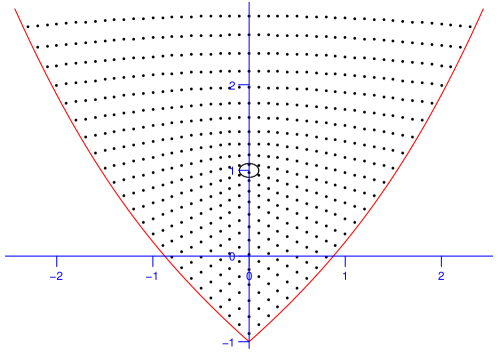
Figure 2: Joint spectrum of the quantum spherical pendulum (black dots) for $\hbar=0.1$. The circle indicates the position of the focus-focus critical value, and the red curve consists of all other critical values of the moment map $(J,H)$. Compare with Figure 1.

Starting from the seminal articles [19, 24], the spherical pendulum has been an inspiring toy-model for the understanding of the many links between classical and quantum integrable systems. The $J$-action is a global $S^{1}$ symmetry, however the spherical pendulum is not strictly speaking a semi-toric system (Definition 5.1), because the function $J$ is not proper. A quantum manifestation of this non-properness can be seen on Figure 2: for each fixed eigenvalue $\mu$ of $\hat{J}$, the corresponding eigenspace is infinite dimensional (and hence there is an infinite number of joint eigenvalues which project down onto $\mu$). Generalized semi-toric systems with non-proper $J$ can behave in many pathological ways, and their classification is still open, see [60].

Spin-oscillator (or Jaynes-Cummings)

It turns out that there is another simple integrable system whose local properties are essentially similar to the spherical pendulum, with the crucial difference that it is a genuine semi-toric system: the so-called spin-oscillator coupling [64], or, in the physics terminology, the Jaynes-Cummings system [39]. It is very similar to the coupled angular momenta of Example 3.18, but it enjoys the additional property, like the spherical pendulum does, to have a non-compact phase space.

Again, we let $S^{2}$ be the unit sphere in $\mathbb{R}^{3}$ with coordinates $(x_{1},\,x_{2},\,x_{3})$, and let $\mathbb{R}^{2}$ be equipped with coordinates $(u,\,v)$. Let $M$ be the product manifold $S^{2}\times\mathbb{R}^{2}$ equipped with the product symplectic structure $\omega_{S^{2}}\oplus\omega_{\mathrm{can}}$, where $\omega_{S^{2}}$ is the standard symplectic form on the sphere and $\omega_{\mathrm{can}}$ is the canonical symplectic form on $\mathbb{R}^{2}$. Let $J,\,H\colon M\to\mathbb{R}$ be the smooth maps defined by

$$J:=(u^{2}+v^{2})/2+z\,\,\textup{and}\,\,H:=\frac{1}{2}\,(ux+vy).$$

The coupled spin-oscillator is the $4$-dimensional integrable system given by $(M,\,\omega_{S^{2}}\oplus\omega_{\mathrm{can}},\,(J,\,H))$. As for the spherical pendulum, the spin-oscillator is an almost-toric system, and it is in fact a semi-toric system (Definition 5.1). Its bifurcation diagram is very similar to that of the spherical pendulum: one isolated focus-focus critical value, and two branches of elliptic-regular values connected to each other at an elliptic-elliptic value.

However, from the quantum viewpoint, the Jaynes-Cummings model is very different the quantum spherical pendulum: because its phase space is not a cotangent bundle, it cannot be quantized using (pseudo)differential operators. Moreover, it contains a compact, invariant symplectic manifold $S^{2}\times\{0\}$, and hence can be quantized only for a discrete set of values of $\hbar\in(0,1]$. There are two natural ways of obtaining commuting operators for this system. One is to view the sphere $S^{2}$ as a symplectic reduction of $\mathbb{C}^{2}$ and use invariant differential operators on $\mathbb{R}^{2}$, see [64]; another possibility is to perform Berezin-Toeplitz quantization of the $S^{2}$, see [59]. Figure 3 shows the joint spectrum of the Jaynes-Cummings model which, as was the case with the spherical pendulum, nicely fits within the image of the classical moment map.

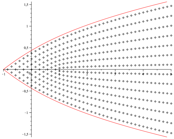
Figure 3: The joint spectrum of the Jaynes-Cummings model (cf. [64, Figure 6]).

6.4 Semiclassical quantization

Following [59], we shall not give the technical details of the Weyl or Berezin-Toeplitz quantization, but instead introduce a minimal set of simple axioms, that are satisfied by these quantizations, and sufficient to understand how to obtain the semiclassical limit of a joint spectrum.

Let $M$ be a connected manifold (either closed or open). Let $\mathcal{A}_{0}$ be a subalgebra of $C^{\infty}(M;\mathbb{R})$ containing the constants and all compactly supported functions. We fix a subset $I\subset(0,1]$ that accumulates at $0$. If $\mathcal{H}$ is a complex Hilbert space, we denote by $\mathcal{L}(\mathcal{H})$ the set of linear (possibly unbounded) selfadjoint operators on $\mathcal{H}$. By a slight abuse of notation, we write $\left\|T\right\|$ for the operator norm of an operator, and $\left\|f\right\|$ for the uniform norm of a function on $M$.

Definition 6.3.

A semiclassical quantization of $(M,\mathcal{A}_{0})$ consists of a family of complex Hilbert spaces $\mathcal{H}_{\hbar},\;\hbar\in I$, and a family of $\mathbb{R}$-linear maps ${\rm Op}_{\hbar}\colon\mathcal{A}_{0}\to\mathcal{L}(\mathcal{H}_{\hbar})$ satisfying the following properties, where $f$ and $g$ are in $\mathcal{A}_{0}$:

1. $\left\|{\rm Op}_{\hbar}(1)-{\rm Id}\right\|=\mathcal{O}(\hbar)$ (normalization);

2. for all $f\geq 0$ there exists a constant $C_{f}$ such that ${\rm Op}_{\hbar}(f)\geq-C_{f}\hbar$ (quasi-positivity); (this means $\langle{\rm Op}_{\hbar}(f)u,u\rangle\geq-C\hbar\left\|u\right\|^{2}$ for all $u\in\mathcal{H}_{\hbar}$)

3. let $f\in\mathcal{A}_{0}$ such that $f\neq 0$ and has compact support, then

   $$\liminf_{\hbar\to 0}\left\|{\rm Op}_{\hbar}(f)\right\|>0$$

   (non-degeneracy);

4. if $g$ has compact support, then for all $f$, ${\rm Op}_{\hbar}(f)\circ{\rm Op}_{\hbar}(g)$ is bounded, and we have

   $$\left\|{\rm Op}_{\hbar}(f)\circ{\rm Op}_{\hbar}(g)-{\rm Op}_{\hbar}(fg)\right\|=\mathcal{O}(\hbar),$$

   (product formula).

A quantizable manifold is a manifold for which there exists a semiclassical quantization.

We shall often use the following consequence of these axioms: for a bounded function $f$, the operator ${\rm Op}_{\hbar}(f)$ is bounded. Indeed, if $c_{1}\leq f\leq c_{2}$ for some $c_{1},c_{2}\in\mathbb{R}$, normalization and quasi-positivity yield

$$c_{1}\cdot\textup{Id}-\mathcal{O}(\hbar)\leq{\rm Op}_{\hbar}(f)\leq c_{2}\cdot\textup{Id}+\mathcal{O}(\hbar).$$ (44)

Since our operators are selfadjoint, this is enough to obtain

$$\left\|{\rm Op}_{\hbar}(f)\right\|\leq\left\|f\right\|+{\mathcal{O}}(\hbar),$$ (45)

see Lemma 6.4 below:

Lemma 6.4.

Let $T$ be a (not necessarily bounded) selfadjoint operator on a Hilbert space with a dense domain and with spectrum $\sigma(T)$, we have

$$\sup\sigma(T)=\sup_{u\neq 0}\frac{\langle Tu,u\rangle}{\langle u,u\rangle}\;.$$ (46)

In particular,

$$\sup\{|s|:s\in\sigma(T)\}=\sup_{u\neq 0}\frac{|\langle Tu,u\rangle|}{\langle u,u\rangle}=\left\|T\right\|\leq\infty;.$$ (47)

Proof.

If $\lambda\in\sigma(T)$, then by the Weyl criterion, there exists a sequence $(u_{n})$ with $\left\|u_{n}\right\|=1$ such that

$$\lim_{n\to\infty}\left\|(T-\lambda{\rm Id})u_{n}\right\|=0.$$

Therefore, $\lim_{n\to\infty}\langle Tu_{n},u_{n}\rangle=\lambda$, which implies that

$$\sup_{\left\|u\right\|=1}\langle Tu,u\rangle\geq\sup\sigma(T).$$

Conversely, if $\sigma(T)$ lies in $(-\infty,c]$, then by the spectral theorem $T\leq c\cdot\textup{Id}$ which yields

$$\sup_{\left\|u\right\|=1}\langle Tu,u\rangle\leq\sup\sigma(T).$$

∎

6.5 Semiclassical operators

Consider the algebra $\mathcal{A}_{I}$ whose elements are collections $\vec{f}=(f_{\hbar})_{\hbar\in I}$, $f_{\hbar}\in\mathcal{A}_{0}$ with the following property: for each ${\vec{f}}$ there exists $f_{0}\in\mathcal{A}_{0}$ so that

$$f_{\hbar}=f_{0}+\hbar f_{1,\hbar}\;,$$ (48)

where the sequence $f_{1,\hbar}$ is uniformly bounded in $\hbar$ and supported in the same compact set $K=K({\vec{f}})\subset M$. The function $f_{0}$ is called the principal part of ${\vec{f}}$. If $f_{0}$ is compactly supported as well, we say that ${\vec{f}}$ is compactly supported.

Definition 6.5.

We define a map

$$\text{Op}:\mathcal{A}_{I}\to\prod_{\hbar\in I}\mathcal{L}(\mathcal{H}_{\hbar}),\;\;{\vec{f}}=(f_{\hbar})\mapsto({\rm Op}_{\hbar}(f_{\hbar}))\;.$$

A semiclassical operator is an element in the image of Op. Given ${\vec{f}}\in\mathcal{A}_{I}$, the function $f_{0}\in\mathcal{A}_{0}$ defined by (48) is called the principal symbol of $\text{Op}({\vec{f}})$.

By (45)

$${\rm Op}_{\hbar}(f_{\hbar})={\rm Op}_{\hbar}(f_{0})+{\mathcal{O}}(\hbar)\;.$$ (49)

This together with the product formula readily yields that for every $\vec{g}$ with compact support and every ${\vec{f}}$,

$$\left\|{\rm Op}_{\hbar}(f_{\hbar})\circ{\rm Op}_{\hbar}(g_{\hbar})-{\rm Op}_{\hbar}(f_{\hbar}g_{\hbar})\right\|=\mathcal{O}(\hbar)\;.$$ (50)

Now we are ready to show that the principal symbol of a semiclassical operator is unique. Indeed, if $\text{Op}({\vec{f}})=0$, then for any compactly supported function $\chi$, we get by (50)

$${\rm Op}_{\hbar}(f_{\hbar}\chi)={\rm Op}_{\hbar}(f_{\hbar}){\rm Op}_{\hbar}(\chi)+\mathcal{O}(\hbar)=\mathcal{O}(\hbar),$$

and then by (49), ${\rm Op}_{\hbar}(f_{0}\chi)=\mathcal{O}(\hbar)$. By the normalization axiom, we conclude that $f_{0}\chi=0$. Since $\chi$ is arbitrary, $f_{0}=0$.

Remark 6.6. It is interesting to notice that this abstract semiclassical quantization does not use the uncertainty principle (43); and in fact, we don’t even require $M$ to be symplectic! This, of course, is necessary for obtaining finer results, see [82].   $\triangle$

6.6 Convergence of the joint spectrum for semiclassical integrable systems

Let $M$ be a quantizable manifold in the sense of Definition 6.3. Following Definition 6.1, we can say that a semiclassical integrable system on $M$ is a set of independent commuting semiclassical operators $(T_{1}(\hbar),\dots,T_{n}(\hbar))$. Here, ‘commuting’ has to be understood for any fixed value of $\hbar$. Let $f_{1},\dots,f_{n}$ be the principal symbols of $T_{1}(\hbar),\dots,T_{n}(\hbar)$, respectively. Then, by definition, the term ‘independent’ means that the differentials $df_{1},\dots,df_{n}$ must be almost everywhere linearly independent, as in Definition 3.10.

Because we have not taken into account, in this weak version of quantization, the Poisson bracket and the uncertainty principle, we cannot relate the commutation $[T_{i}(\hbar),T_{j}(\hbar)]=0$ to a classical property. In fact, in the very general theorem below, we don’t even need the independence of $T_{1}(\hbar),\dots,T_{n}(\hbar)$. In any case, we may define the joint spectrum $\Sigma_{\hbar}(T_{1},\dots,T_{d})$, see Definition 6.2.

Theorem 6.7 ([59]).

Let $M$ be a quantizable manifold. Let $d\geq 1$ and let $(T_{1},\dots T_{d})$ be pairwise commuting semiclassical operators on $M$. Let $F=(f_{1},\dots,f_{n}):M\to\mathbb{R}^{n}$, where $f_{j}$ is the principal symbol of $T_{j}$. Let $J$ be a subset of $I$ that accumulates at $0$. Then from the family

$$\Big{\{}\Sigma_{\hbar}(T_{1},\dots,T_{d})\Big{\}}_{\hbar\in J}$$

one can recover the closed convex hull of $F(M)$.

The theorem is in fact constructive, in the sense that the convex hull of $\Sigma_{\hbar}(T_{1},\dots,T_{d})$ converges locally, in the Hausdorff sense, to $F(M)$; more precisely, we have:

Theorem 6.8 ([59]).

Under the hypothesis of Theorem 6.7, if the operators $T_{j}$ are uniformly bounded as $\hbar\to 0$, then the closed convex hull of $\Sigma_{\hbar}(T_{1},\dots,T_{d})$ converges in the Hausdorff metric, as $\hbar\to 0$, to the closed convex hull of $F(M)$.

Proof.

We restrict here to the one-dimensional case ($n=1$); the general case can be recovered by using linear combinations of the form $T_{\xi}:=\sum\xi_{j}T_{j}$ (see [59]). If $n=1$, the statement is quite easy to write down:

«Prove that

$$[\inf\sigma(T),\sup\sigma(T)]\to[\inf f,\sup f]\quad\text{ as }{\hbar\to 0},$$

where $T$ is a bounded semiclassical operator, and $f$ its principal symbol.»

Let $\epsilon>0$ be fixed, independent on $\hbar$. The easy part is to prove that, when $\hbar$ is small enough,

$$\sup\sigma(T)\leq\sup f+\epsilon,$$

as this is a direct consequence of (45), (46), and (47). Now let us show that, conversely,

$$\sup\sigma(T)\geq\sup f-2\epsilon.$$

The strategy is to construct a good ‘test function’ $u$ that is close to realizing the $\sup$ in (46). Let $F_{\epsilon}:=\sup f-\epsilon$; since $f$ is continuous, there exists a connected open set $B\subset M$ where $f\geq F_{\epsilon}$. Let $\chi\geq 0$ with $\chi\in C^{\infty}_{0}(B)$, i.e. $\chi$ is smooth function on $M$ with compact support $K\subset B$. Thus $(f-F_{\epsilon})\chi\geq 0$ on $M$ and $(f-F_{\epsilon})\chi=0$ outside of $K$ (see Figure 4). Let $\tilde{\chi}$ be another cut-off function, with $\tilde{\chi}\geq 0$, $\tilde{\chi}=1$ on a open set $\tilde{B}$ whose closure is contained in $B$, and $\tilde{\chi}\in C^{\infty}_{0}(K)$, so that $\tilde{\chi}\chi=\tilde{\chi}$, and hence, by the product formula,

$${\rm Op}_{\hbar}\chi\circ{\rm Op}_{\hbar}\tilde{\chi}={\rm Op}_{\hbar}\chi\tilde{\chi}+\mathcal{O}(\hbar)={\rm Op}_{\hbar}\tilde{\chi}+\mathcal{O}(\hbar).$$ (51)

Figure 4: Construction of the ‘quasimode’ $w_{\hbar}$

The non-degeneracy axiom, together with Lemma 6.4, implies that one can find a vector $v_{\hbar}\in\mathcal{H}_{\hbar}$ such that

$$\left\|({\rm Op}_{\hbar}\tilde{\chi})v_{\hbar}\right\|>c/2,\qquad c=\left\|{\rm Op}_{\hbar}\tilde{\chi}\right\|,$$

uniformly in $\hbar\leq 1$. Let

$$u_{\hbar}:=\frac{({\rm Op}_{\hbar}\tilde{\chi})v_{\hbar}}{\left\|({\rm Op}_{\hbar}\tilde{\chi})v_{\hbar}\right\|};$$

then, using (51), we obtain

$$({\rm Op}_{\hbar}\chi)u_{\hbar}=u_{\hbar}+\mathcal{O}(\hbar).$$

Finally, let $w_{\hbar}:=({\rm Op}_{\hbar}\chi)u_{\hbar}$; we have

$${\rm Op}_{\hbar}(f-F_{\epsilon})w_{\hbar}={\rm Op}_{\hbar}((f-F_{\epsilon})\chi)u_{\hbar}+\mathcal{O}(\hbar).$$

Hence, the quasi-positivity axiom implies

$$\langle{\rm Op}_{\hbar}(f-F_{\epsilon})w_{\hbar},u_{\hbar}\rangle\geq-C_{\epsilon}\hbar\left\|u_{\hbar}\right\|,$$

for some constant $C_{\epsilon}$ depending on $\epsilon$. Since $\left\|u_{\hbar}\right\|=1$ and $\left\|w_{\hbar}\right\|=1+\mathcal{O}(\hbar)$, we get, for a possibly different constant $\tilde{C}_{\epsilon}$,

$$\langle{\rm Op}_{\hbar}(f-F_{\epsilon})w_{\hbar},w_{\hbar}\rangle\geq-\tilde{C}_{\epsilon}\hbar\left\|u_{\hbar}\right\|,$$

which implies, due to Lemma 6.4, that $\sup\sigma(T)\geq F_{\epsilon}-\tilde{C}_{\epsilon}\hbar$. Thus, when $\hbar$ is small enough, we can reach

$$\sup\sigma(T)\geq F_{\epsilon}-\epsilon,$$

as required. ∎

6.7 The inverse problem in the toric case

Theorem 6.7 has a rather spectacular consequence in the case of toric systems. Recall that an integrable system is called toric if the Hamiltonian flow of each function $f_{1},\dots,f_{n}$ is $2\pi$-periodic, and the corresponding $\mathbb{T}^{n}$-action is effective, see Example 3.19. Accordingly, a set of commuting semiclassical operators $T_{1},\dots,T_{n}$ will, by definition, constitute a quantum toric system if the principal symbols $f_{1},\dots,f_{n}$ form a toric system.

Such systems have been studied in details in [11] in the framework of Berezin-Toeplitz quantization. It was proven that the joint spectrum of such a system is a regular deformation (in the semiclassical parameter $\hbar$) of the set of $\hbar$-integral points of the image of the moment map $\mu:=(f_{1},\dots,f_{n})$; precisely:

$$\Sigma_{\hbar}(T_{1},\dots,T_{n})=g_{\hbar}(\mu(M)\cap(v+\hbar\mathbb{Z}^{n}))+\mathcal{O}(\hbar^{\infty}),$$

where $v$ is any vertex of the polytope $\mu(M)$, and $g_{\hbar}$ is a deformation of the identity:

$$g_{h}=\textup{Id}+\hbar g_{1}+\hbar^{2}g_{2}+\cdots,$$

in the sense of an asymptotic expansion in the $C^{\infty}(\mathbb{R}^{n})$ topology.

As a consequence, the inverse problem was solved; in fact, this also follows directly from Theorem 6.7 for a general semiclassical quantization:

Theorem 6.9 ([11, 59]).

In the class of quantum toric systems (on a compact symplectic manifold $M$), the asymptotics of the joint spectrum completely determines the symplectic manifold $M$ and the toric moment map $\mu$.

Proof.

The proof is a simple application of Theorem 6.7, in view of the Delzant classification [22]. Indeed, the asymptotics of the joint spectrum determine the closed convex hull of $\mu(M)$. But we know that in the class of toric systems, the image $\mu(M)$ is closed and convex. Thus, we may recover $\mu(M)$ from the joint spectrum. By the Delzant result, $\mu(M)$ in turn completely determines $(M,\mu)$. ∎

6.8 The general inverse problem

In view of Theorem 6.9 above, it is tempting to state a general conjecture (which is a slight refinement of the statements in [65, Conjecture 9.1], [66, Conjecture 3.4]), as follows:

Conjecture 6.10.

Let $\mathscr{N\!D}_{n}$ be the class of completely integrable systems on a $2n$ symplectic manifold with non-degenerate singularities (see Definition 4.7). Let $Q(\mathscr{N\!D}_{n})$ be the class of $n$-uples $T=(T_{1},\dots,T_{n})$ of commuting operators whose principal symbols form an element in $\mathscr{N\!D}_{n}$. Then the asymptotics of the joint spectrum of an element in $T\in Q(\mathscr{N\!D}_{n})$ completely determines the symplectic manifold and the principal symbols of $T$.

At the time of writing, this conjecture is open. However, preliminary results can shed some light. In one degree of freedom, the conjecture was shown to hold in a generic (and large) subset of $\mathscr{N\!D}_{1}$ [83]. Genericity was necessary because of possible symmetries that generate eigenvalues with multiplicities. Hence, for a general statement, it should be clear that ‘joint spectrum’ is understood as a spectrum with multiplicities.

Theorem 6.9 states that the conjecture holds when $\mathscr{N\!D_{n}}$ is replaced by the set of toric systems. Recently, several papers have been trying to attack the semi-toric case (which was already formulated as a conjecture in [65], cf. [66, 46] and references therein). In [46], the authors prove the following result:

Theorem 6.11 ([46]).

For quantum semi-toric systems which are either semiclassical pseudo-differential operators, or semiclassical Berezin-Toeplitz operators, the joint spectrum (modulo $\mathcal{O}(\hbar^{2})$) determines the following invariants:

1. the number $m_{f}$ of focus-focus values,

2. the Taylor series invariant (see Definition 5.12),

3. the volume invariant associated with each focus-focus value,

4. the polygonal invariant of the system.

The last two ingredients are part of what we describe in this work as the cartographic invariant, see Section 5.2. In order to obtain a full answer in the semi-toric case, it remains on the one hand to be able to detect the full cartographic invariant (which means detecting the twisting cocycle), and on the other hand to recover exactly the principal symbols, not only up to isomorphism (in other words, if two systems have the same joint spectrum, can we prove that the map $g$ in Definition 5.7 is the identity?).

In comparison to semi-toric systems, more general integrable systems in $\mathscr{N\!D}_{n}$ become quickly much more delicate to analyze, due to the presence of hyperbolic singularities, which allow for non-connected fibers of the moment map. It is currently not known how to obtain a tractable classification of integrable systems with hyperbolic singularities; however a solid topological foundation was laid out in the book [7]. A reasonable approach would be to first consider the case of hyperbolic singularities in the presence of a global $S^{1}$-action.

Finally, we conclude with two open questions closely related to the conjecture.

1. Can one detect from the joint spectrum of a system in $Q(\mathscr{N\!D}_{n})$ whether the system is semi-toric?

2. Can one tell from the joint spectrum of a general quantum integrable system whether it belongs to $Q(\mathscr{N\!D}_{n})$?

References

- [1] D. V. Anosov. Geodesic flows on closed Riemann manifolds with negative curvature. Proceedings of the Steklov Institute of Mathematics, No. 90 (1967). Translated from the Russian by S. Feder. American Mathematical Society, Providence, R.I., 1969.
- [2] M. F. Atiyah. Convexity and commuting Hamiltonians. Bull. London Math. Soc., 14(1):1–15, 1982.
- [3] L. Auslander and L. Markus. Holonomy of flat affinely connected manifolds. Ann. of Math. (2), 62:139–151, 1955.
- [4] W. Ballmann. Lectures on spaces of nonpositive curvature, volume 25 of DMV Seminar. Birkhäuser Verlag, Basel, 1995. With an appendix by Misha Brin.
- [5] L. M. Bates and J. Śniatycki. On action-angle variables. Arch. Rational Mech. Anal., 120(4):337–343, 1992.
- [6] A. Bolsinov and A. Izosimov. Smooth invariants of focus-focus singularities and obstructions to product decomposition. arXiv: 1706.07456, 2017.
- [7] A. V. Bolsinov and A. T. Fomenko. Integrable Hamiltonian systems; Geometry, topology, classification. Chapman & Hall, 2004. Translated from the 1999 Russian original.
- [8] M. Chaperon. Normalisation of the smooth focus-focus: a simple proof. Acta Math. Vietnam., 38(1):3–9, 2013.
- [9] A.-M. Charbonnel. Comportement semi-classique du spectre conjoint d’opérateurs pseudo-différentiels qui commutent. Asymptotic Analysis, 1:227–261, 1988.
- [10] L. Charles. Berezin-Toeplitz operators, a semi-classical approach. Commun. Math. Phys., 239(1-2):1–28, 2003.
- [11] L. Charles, Á. Pelayo, and S. Vũ Ngọc. Isospectrality for quantum toric integrable systems. Ann. Sci. École Norm. Sup., 43:815–849, 2013.
- [12] M. S. Child. Quantum states in a champagne bottle. J.Phys.A., 31:657–670, 1998.
- [13] M. S. Child, T. Weston, and J. Tennyson. Quantum monodromy in the spectrum of H2O and other systems: new insight into the level structure of quasi-linear molecules. Mol. Phys., 96(3):371–379, 1999.
- [14] Y. Colin de Verdière and S. Vũ Ngọc. Singular Bohr-Sommerfeld rules for 2D integrable systems. Ann. Sci. École Norm. Sup. (4), 36(1):1–55, 2003.
- [15] Y. Colin de Verdière and J. Vey. Le lemme de Morse isochore. Topology, 18(4):283–293, 1979.
- [16] M. Crainic, R. Loja Fernandes, and D. Martínez-Torres. Regular Poisson manifolds of compact types (PMCT2). arXiv:1603.00064, 2016.
- [17] M. Crainic, R. Loja Fernandes, and D. Martínez-Torres. Poisson manifolds of compact types (PMCT1). to appear in Journal für die reine und angewandte Mathematik (Crelle), 2017.
- [18] F. W. Cummings. Stimulated emission of radiation in a single mode. Phys. Rev., 140(4A):A1051–A1056, 1965.
- [19] R. Cushman and J. J. Duistermaat. The quantum spherical pendulum. Bull. Amer. Math. Soc. (N.S.), 19:475–479, 1988.
- [20] R. Cushman, H. Dullin, A. Giacobbe, D. Holm, M. Joyeux, P. Lynch, D. Sadovskii, and B. Zhilinskii. The molecule as a quantum realization of the resonant swing-spring with monodromy. Phys. Rev. Lett., 93(24302), 2004.
- [21] P. Dazord and T. Delzant. Le problème général des variables actions-angles. J. Differential Geom., 26(2):223–251, 1987.
- [22] T. Delzant. Hamiltoniens périodiques et images convexes de l’application moment. Bull. Soc. Math. France, 116(3):315–339, 1988.
- [23] J.-P. Dufour and P. Molino. Compactification d’actions de et variables action-angle avec singularités. In Symplectic geometry, groupoids, and integrable systems (Berkeley, CA, 1989), volume 20 of Math. Sci. Res. Inst. Publ., pages 151–167. Springer, New York, 1991.
- [24] J. J. Duistermaat. On global action-angle coordinates. Comm. Pure Appl. Math., 33(6):687–706, 1980.
- [25] J. J. Duistermaat and G. J. Heckman. On the variation in the cohomology of the symplectic form of the reduced phase space. Invent. Math., 69(2):259–268, 1982.
- [26] H. R. Dullin. Semi-global symplectic invariants of the spherical pendulum. J. Differential Equations, 254(7):2942–2963, 2013.
- [27] L. H. Eliasson. Hamiltonian systems with Poisson commuting integrals. PhD thesis, University of Stockholm, 1984.
- [28] L. H. Eliasson. Normal forms for Hamiltonian systems with Poisson commuting integrals—elliptic case. Comment. Math. Helv., 65(1):4–35, 1990.
- [29] R. L. Fernandes, C. Laurent-Gengoux, and P. Vanhaecke. Global action-angle variables for non-commutative integrable systems. to appear in J. Symp. Geom., 2015.
- [30] V. Guillemin, E. Lerman, and S. Sternberg. On the Kostant multiplicity formula. J. Geom. Phys., 5(4):721–750 (1989), 1988.
- [31] V. Guillemin and S. Sternberg. Convexity properties of the moment mapping. Invent. Math., 67(3):491–513, 1982.
- [32] V. Guillemin and S. Sternberg. Symplectic techniques in physics. Cambridge University Press, Cambridge, second edition, 1990.
- [33] V. Guillemin and S. Sternberg. Semi-classical analysis. International Press, Boston, MA, 2013.
- [34] H. Hofer and E. Zehnder. Symplectic invariants and Hamiltonian dynamics. Birkhäuser Advanced Texts: Basler Lehrbücher. Birkhäuser Verlag, Basel, 1994.
- [35] S. Hohloch, S. Sabatini, and D. Sepe. From compact semi-toric systems to Hamiltonian -spaces. Discrete Contin. Dyn. Syst., 35(1):247–281, 2015.
- [36] S. Hohloch, S. Sabatini, D. Sepe, and M. Symington. From Hamiltonian -spaces to compact semi-toric systems via surgeries. In preparation, 2017.
- [37] S. Hohloch, S. Sabatini, D. Sepe, and M. Symington. Vertical almost-toric systems. ArXiv:1706.09935, 2017.
- [38] C. Huygens. Horologium Oscillatorium sive de motu pendulorum. Muguet, Paris, 1673.
- [39] E. T. Jaynes and F. W. Cummings. Comparison of quantum and semiclassical radiation theories with application to the beam maser. Proc. IEEE, 51(1):89–109, 1963.
- [40] B. Jovanović. Noncommutative integrability and action-angle variables in contact geometry. J. Symplectic Geom., 10(4):535–561, 2012.
- [41] M. Joyeux. Gustavson’s procedure and the dynamics of highly excited vibrational states. J. Chem. Phys., 109:2111–2122, 1998.
- [42] Y. Karshon. Periodic Hamiltonian flows on four-dimensional manifolds. Mem. Amer. Math. Soc., 141(672):viii+71, 1999.
- [43] Y. Karshon and E. Lerman. Non-compact symplectic toric manifolds. SIGMA Symmetry Integrability Geom. Methods Appl., 11:Paper 055, 37, 2015.
- [44] L. D. Landau and E. M. Lifshitz. Quantum mechanics: non-relativistic theory. Course of Theoretical Physics, Vol. 3. Addison-Wesley Series in Advanced Physics. Pergamon Press Ltd., London-Paris; for U.S.A. and Canada: Addison-Wesley Publishing Co., Inc., Reading, Mass;, 1958. Translated from the Russian by J. B. Sykes and J. S. Bell.
- [45] Y. Le Floch, J. Palmer, D. Sepe, and S. Vũ Ngọc. Integrable systems, symmetries, and quantization – exercises with solutions. Poisson 2016 Summer School, available at https://tinyurl.com/n4qjsm5, 2016.
- [46] Y. Le Floch, Á. Pelayo, and S. Vũ Ngọc. Inverse spectral theory for semiclassical Jaynes-Cummings systems. Math. Ann., 364(3):1393––1413, 2016.
- [47] E. Lerman, E. Meinrenken, S. Tolman, and C. Woodward. Nonabelian convexity by symplectic cuts. Topology, 37(2):245–259, 1998.
- [48] X. Ma and G. Marinescu. Holomorphic Morse inequalities and Bergman kernels, volume 254 of Progress in Mathematics. Birkhäuser Verlag, Basel, 2007.
- [49] V. S. Matveev. Integrable Hamiltonian systems with two degrees of freedom. Topological structure of saturated neighborhoods of points of focus-focus and saddle-saddle types. Mat. Sb., 187(4):29–58, 1996.
- [50] D. McDuff and D. Salamon. Introduction to symplectic topology. Oxford Mathematical Monographs. The Clarendon Press, Oxford University Press, New York, second edition, 1998.
- [51] H. Mineur. Sur les systèmes mécaniques dans lesquels figurent des paramètres fonctions du temps. Étude des systèmes admettant intégrales premières uniformes en involution. Extension à ces systèmes des conditions de quantification de Bohr-Sommerfeld. J. Ecole Polytechn., III(Cahier 1, Fasc. 2 et 3):173–191, 237–270, 1937.
- [52] E. Miranda. On symplectic linearization of singular Lagrangian foliations. PhD thesis, University of Barcelona, 2003.
- [53] E. Miranda and S. Vũ Ngọc. A singular Poincaré lemma. Int. Math. Res. Not., 1:27–45, 2005.
- [54] E. Miranda and N. T. Zung. Equivariant normal form for nondegenerate singular orbits of integrable Hamiltonian systems. Ann. Sci. École Norm. Sup. (4), 37(6):819–839, 2004.
- [55] I. Moerdijk and J. Mrčun. Introduction to foliations and Lie groupoids, volume 91 of Cambridge Studies in Advanced Mathematics. Cambridge University Press, Cambridge, 2003.
- [56] J. Mrčun. An extension of the Reeb stability theorem. Topology Appl., 70(1):25–55, 1996.
- [57] R. S. Palais. The symmetries of solitons. Bull. Amer. Math. Soc. (N.S.), 34(4):339–403, 1997.
- [58] G. Papadopoulos and H. R. Dullin. Semi-global symplectic invariants of the Euler top. J. Geom. Mech., 5(2):215–232, 2013.
- [59] Á. Pelayo, L. Polterovich, and S. Vũ Ngọc. Semiclassical quantization and spectral limits of -pseudodifferential and Berezin-Toeplitz operators. Proc. Lond. Math. Soc. (3), 109(3):676–696, 2014.
- [60] Á. Pelayo, T. Ratiu, and S. Vũ Ngọc. The affine invariant of generalized semitoric systems. Nonlinearity, 2017. To appear.
- [61] Á. Pelayo and X. Tang. Vũ Ngọc’s conjecture on focus-focus singularities with multiple pinched points. In preparation.
- [62] Á. Pelayo and S. Vũ Ngọc. Semitoric integrable systems on symplectic 4-manifolds. Invent. Math., 177(3):571–597, 2009.
- [63] Á. Pelayo and S. Vũ Ngọc. Constructing integrable systems of semitoric type. Acta Math., 206(1):93–125, 2011.
- [64] Á. Pelayo and S. Vũ Ngọc. Hamiltonian dynamics and spectral theory for spin-oscillators. Comm. Math. Phys., 309(1):123–154, 2012.
- [65] Á. Pelayo and S. Vũ Ngọc. Symplectic theory of completely integrable Hamiltonian systems. Bull. Amer. Math. Soc. (N.S.), 48(3):409–455, 2011.
- [66] Á. Pelayo and S. Vũ Ngọc. First steps in symplectic and spectral theory of integrable systems. Discrete Contin. Dyn. Syst., 32(10):3325–3377, 2012.
- [67] H. Rüssmann. Über das Verhalten analytischer Hamiltonscher Differentialgleichungen in der Nähe einer Gleichgewichtslösung. Math. Ann., 154:285–300, 1964.
- [68] D. A. Sadovskií and B. I. Zĥilinskií. Monodromy, diabolic points, and angular momentum coupling. Phys. Lett. A, 256(4):235–244, 1999.
- [69] M. A. Salazar and D. Sepe. Contact isotropic realisations of Jacobi manifolds via Spencer operators. SIGMA, 13(033):44 pages, 2017.
- [70] N. Sansonetto and D. Sepe. Twisted isotropic realisations of twisted Poisson structures. J. Geom. Mech., 5(2):233–256, 2013.
- [71] J. Smillie. An obstruction to the existence of affine structures. Invent. Math., 64(3):411–415, 1981.
- [72] G. Smirnov. Focus-focus singularities in classical mechanics. Nelin. Dinam., 10(1):101–112, 2014.
- [73] I. Stewart. Quantizing the classical cat. Nature, 430:731–732, 2004.
- [74] M. Symington. Four dimensions from two in symplectic topology. In Topology and geometry of manifolds (Athens, GA, 2001), volume 71 of Proc. Sympos. Pure Math., pages 153–208. Amer. Math. Soc., Providence, RI, 2003.
- [75] M. E. Taylor. Partial differential equations II. Qualitative studies of linear equations, volume 116 of Applied Mathematical Sciences. Springer, New York, second edition, 2011.
- [76] S. Vũ Ngọc. Bohr-Sommerfeld conditions for integrable systems with critical manifolds of focus-focus type. Comm. Pure Appl. Math., 53(2):143–217, 2000.
- [77] S. Vũ Ngọc. On semi-global invariants for focus-focus singularities. Topology, 42(2):365–380, 2003.
- [78] S. Vũ Ngọc. Moment polytopes for symplectic manifolds with monodromy. Adv. Math., 208(2):909–934, 2007.
- [79] S. Vũ Ngọc and C. Wacheux. Smooth normal forms for integrable Hamiltonian systems near a focus-focus singularity. Acta Math. Vietnam., 38(1):107–122, 2013.
- [80] J. Vey. Sur certains systèmes dynamiques séparables. Amer. J. Math., 100(3):591–614, 1978.
- [81] S. Vũ Ngọc. Formes normales semi-classiques des systèmes complètement intégrables au voisinage d’un point critique de l’application moment. Asymptotic Analysis, 24(3,4):319–342, 2000.
- [82] S. Vũ Ngọc. Systèmes intégrables semi-classiques: du local au global. Number 22 in Panoramas et Syhthèses. SMF, 2006.
- [83] S. Vũ Ngọc. Symplectic inverse spectral theory for pseudodifferential operators. In Geometric aspects of analysis and mechanics, volume 292 of Progr. Math., pages 353–372. Birkhäuser/Springer, New York, 2011.
- [84] R. Wang. On Integrable Systems and Rigidity for PDEs with Symmetry. PhD thesis, Utrecht Universiteit, 2017.
- [85] A. Weinstein. Symplectic manifolds and their lagrangian submanifolds. Adv. Math., 6:329 – 346, 1971.
- [86] A. Weinstein. Symplectic geometry. Bull. Amer. Math. Soc. (N.S.), 5(1):1–13, 1981.
- [87] A. Weinstein. The local structure of Poisson manifolds. J. Differential Geom., 18(3):523–557, 1983.
- [88] J. Williamson. On the Algebraic Problem Concerning the Normal Forms of Linear Dynamical Systems. Amer. J. Math., 58(1):141–163, 1936.
- [89] J. Williamson. An algebraic problem involving the involutory integrals of linear dynamical systems. Amer. J. Math., 62:881–911, 1940.
- [90] M. Zou. Monodromy in two degrees of freedom integrable systems. J. Geom. Phys., 10:37–45, 1992.
- [91] N. T. Zung. Symplectic topology of integrable Hamiltonian systems. I. Arnold-Liouville with singularities. Compositio Math., 101(2):179–215, 1996.
- [92] N. T. Zung. A note on focus-focus singularities. Differential Geom. Appl., 7(2):123–130, 1997.
- [93] N. T. Zung. Another note on focus-focus singularities. Lett. Math. Phys., 60(1):87–99, 2002.
- [94] N. T. Zung. Symplectic topology of integrable Hamiltonian systems. II. Topological classification. Compositio Math., 138(2):125–156, 2003.
- [95] N. T. Zung. Proper groupoids and momentum maps: linearization, affinity, and convexity. Ann. Sci. École Norm. Sup. (4), 39(5):841–869, 2006.
- [96] M. Zworski. Semiclassical analysis, volume 138 of Graduate Studies in Mathematics. American Mathematical Society, Providence, RI, 2012.